Quaderni dell’Ufficio Ricerche Storiche

Production and Consumptionin Post-Unification Italy:

New Evidence, New Conjectures

by Stefano Fenoaltea

Number 5 - June 2002

The purpose of the Quaderni dell’Ufficio Ricerche Storiche is to promote thecirculation of working papers prepared within the Bank of Italy or presented in Bankseminars by outside speakers with the aim of stimulating comments and suggestions.

The views expressed in the articles are those of the authors and do not involve theresponsibility of the Bank.

Editorial Board:FILIPPO CESARANO, SERGIO CARDARELLI, STEFANO FENOALTEA, ALFREDO GIGLIOBIANCO,

JUAN CARLOS MARTINEZ OLIVA; GIULIANA FERRETTI (Editorial Assistant).

PRODUCTION AND CONSUMPTIONIN POST-UNIFICATION ITALY:

NEW EVIDENCE, NEW CONJECTURES

by Stefano Fenoaltea∗

Abstract

It is widely believed that in the 1880s falling grain prices immiserized the rural world,dragged down the entire economy, and caused massive emigration. This paper argues thatthe 1880s were actually prosperous; that the fall in the price of imported grain was generallybeneficial; and that rising emigration was due to improving opportunities abroad. Thedecline in consumption registered by the national accounts is due entirely to the notoriouslyspurious grain-consumption series. The better statistical evidence related to imported foods,textiles, and wages in industry and agriculture points uniformly to cyclically high incomesand consumption, and the anthropometric data show no evidence of widespread hardship.Grain and total food consumption were therefore presumably also above trend. In fact, onlylandowners appear to have been damaged by the fall in grain prices; but their voicedominates the record.

∗ Università di Brescia, Dipartimento di scienze economiche

Contents

1. Introduction....................................................................................................................... 9 2. The pessimist presumptions: supply shocks and crises.................................................. 11 3. The pessimist presumptions: living standards and migration......................................... 13 4. The statistical evidence: the consumption of grain ........................................................ 15 5. The statistical evidence: the consumption of other foods............................................... 17 6. The statistical evidence: the consumption of textiles..................................................... 20 7. The statistical evidence: the real wages of skilled labor in industry.............................. 22 8. The statistical evidence: the real wages of unskilled labor in industry and

agriculture........................................................................................................................ 25 9. The statistical evidence: heights ..................................................................................... 2710. New conjectures: food consumption in the 1880s.......................................................... 2811. New conjectures: the construction of the “agrarian crisis” ............................................ 30Appendix A. An improved cost of living index, 1861-1913 ................................................. 31Appendix B. Wage series for unskilled workers, 1861-1913................................................ 34

B.1 Methodological issues .............................................................................................. 34B.2 An index of the nominal wages of unskilled industrial workers.............................. 37B.3 An index of the nominal wages of agricultural workers .......................................... 40

Tables1. Beer, coffee and sugar: annual per-capita consumption, prices and spending,

1861-1913................................................................................................................. 422. Beer, coffee and sugar: decadal average per-capita consumption, prices and

spending, 1861-1913 ................................................................................................ 443. Cotton and wool: annual per-capita fiber consumption, prices and spending,

1861-1913................................................................................................................. 454. Cotton and wool: decadal average per-capita fiber consumption, prices and

spending, 1861-1913 ................................................................................................ 475. Nominal and real wages of skilled industrial workers, 1861-1913.......................... 486. Nominal and real wages of unskilled workers in industry and agriculture,

1861-1913................................................................................................................. 507. Height of draft-eligible males, by year of birth, 1861-1913..................................... 52A.1 Price indices, 1861-1914.......................................................................................... 54B.1 Unskilled adult male workers’ wages, 1861-1913................................................... 56

Figures1. Per-capita beer consumption.................................................................................... 582. Coffee prices, consumption and spending................................................................ 593. Sugar prices, consumption and spending ................................................................. 604. Cotton prices, consumption and spending................................................................ 615. Wool prices, consumption and spending.................................................................. 626. Annuario wage series ............................................................................................... 637. Wages in construction and silk-reeling .................................................................... 648. Wages of unskilled workers ..................................................................................... 65A.1 Istat price indices and a bread-and-flour price index ............................................... 66A.2 Alternative cost of living indices.............................................................................. 67

References............................................................................................................................... 68

1. Introduction1

From the depths of the depression of the mid-1890s to the outbreak of the Great War

Italy experienced, by all accounts, two decades of increasing prosperity. Wages and stock

prices rose, the budget moved into surplus, the exchange rate returned to par, interest rates

fell, construction boomed, agriculture prospered, and manufacturing grew vigorously enough

to convince Gerschenkron that those were the years of Italy’s “big push” (Fenoaltea, 1988a;

Gerschenkron, 1962, pp. 72-89; Toniolo, 1988, pp. 159-97).

The decade of the 1880s is instead altogether less clear-cut. Construction and

manufacturing appear to have done well, and industrial wages at least appear to have risen; but

those were also the years of the “agrarian crisis” induced in Italy as elsewhere in Europe by the

dramatic fall in the price of imported grain. In the face of these intersectoral contrasts, which

Toniolo’s recent text calls “the contradictions of the 1880s” (Toniolo, 1988, pp. 119-37), an

overall assessment is not easily obtained; and since the statistical evidence is too limited in

quantity and in quality to resolve the issue directly, the 1880s lend themselves to widely

differing interpretations.

To the now hegemonic “pessimist” school, the agrarian crisis was the defining feature of

the decade: the sharp fall in grain prices immiserized the rural world, dragged down the entire

economy, and caused the upsurge in emigration. The decline in per-capita consumption

implied by the national income series is accepted as evidence of widespread hardship; the duty

on grain introduced in 1887 is praised as an effective means of limiting rural suffering and

emigration.

The contrasting “optimist” view, heir to an older tradition, sees the agrarian crisis as one

affecting land-owners rather than rural laborers; doubts that agricultural wages were falling,

given that industrial wages were rising; dismisses the registered decline in per-capita

1 The author would like to thank Elio Cerrito, Juan Carlos Martinez Oliva, and the participants at the

Seminario sui consumi (Università di Venezia, 2000), including in particular Giovanni Federico, for theircomments. He is also grateful for the financial support received from the Università di Brescia and the Ministerodell’Università e della Ricerca Scientifica e Tecnologica (research project on “Growth, Welfare and Consumptionin Italy, 1861-2000”). The usual disclaimer applies.

10

consumption as a statistical fiction; attributes the high emigration of the 1880s essentially to

improved opportunities abroad, as after the turn of the century, and denies that grain protection

contained it.

At one level, therefore, this disagreement continues the century-old dispute over the

merits and demerits of Italy’s tariff policy; at another, it emphasizes the need to reconsider the

time path of late nineteenth-century Italy’s statistical aggregates; and at yet another it may well

reflect the clash not just of different interpretations but of different mind-sets and approaches

to our craft.

This paper seeks to bring this “standard of living” debate explicitly into the literature,

and to retake the high ground for the optimists. Sections 2 and 3 challenge the presumptions

that underlie the pessimist position: that the fall in grain prices would cause a general crisis in

and beyond agriculture, and that rising emigration points to rising hardship. Sections 4, 5 and

6 discuss the statistical evidence of consumption; the pessimist position is supported only by

the notoriously unreliable grain series, while the more reliable figures for other foods and

textiles point uniformly to rising living standards in the 1880s as in the early 1900s. Sections

7, 8 and 9 consider the available evidence on real wages and heights: skilled and unskilled

workers in industry and rural day-laborers too appear to have prospered in the 1880s as after

the turn of the century, and the anthropometric evidence reveals no sign of a deterioration at

the bottom of the scale. Sections 10 and 11 are devoted to concluding considerations. The

former argues that in the 1880s food consumption in general, and grain consumption too, were

more plausibly above trend rather than, as the official series now have them, below trend. The

latter suggests that the notion of a general “agrarian crisis” gained currency only because the

surviving record overrepresents the particular interests of the land-owners; but that too is not

without distinguished precedent.

The Appendices describe the construction of an improved cost of living index, and of

wage series for unskilled workers in industry and agriculture.

11

2. The pessimist presumptions: supply shocks and crises

Early twentieth-century economists and historians described the 1880s as “a period of

general prosperity”; but that was long ago.2

The opposite, “pessimist” view dominates the more recent literature: it may be found for

example in the pioneering efforts of Romeo and Luzzatto in the 1950s and ’60s, more recently

in Zamagni’s masterly text, and more recently still, in particularly dramatic terms, in

Castronovo’s survey.3 The underlying syllogism is simple, superficially compelling, and

rhetorically unbeatable. From 1880 to 1885 grain prices fell by a third.4 The fall in grain

prices, it is argued, hurt grain-growing; grain-growing was a major part of agriculture, so

agriculture as a whole suffered (the “agrarian crisis”); agriculture was the economy’s dominant

sector, so the entire economy suffered (the general crisis of the 1880s). Living standards

therefore fell; deepening poverty caused, and is confirmed by, the upsurge in emigration. This

last point is icing, and will be considered below; the cake is the preceding part.

One’s expectations about the extent and significance of the “agrarian crisis” may

however be shaped by different considerations altogether. The fall in grain prices was due to

the competition of imports; and those of us whose remaining hair is gray have experienced in

our own lifetimes the effects of severe variations in the price of a basic import.

Recall the shocks the Western economies experienced at the hands of the international

oil cartel. The absolute and relative price of a basic imported good rose dramatically, with

differential effects on a series of markets, and a consequent reallocation of resources out of the

sectors which were badly hit and into those that reaped benefits. In the large, however, for the

West the rise in the price of imported oil signified a sharp deterioration in the terms of trade,

2 The citation is from Croce (1967, p. 46, my translation). This pocket edition reproduces the author’s prefaces

from the first and ninth editions, dated 1927 and 1949, respectively. A similar evaluation appears in Sensini(1904, p. 23). This remarkable work, kindly brought to my attention by Pierluigi Ciocca, closely anticipates manyof the arguments presented here.

3 Romeo (1963, pp. 165-71); Luzzatto (1968, pp. 168-73); Zamagni (1990, pp. 83-84, 153); Castronovo (1995,pp. 51-53). The account in Toniolo (1988, pp. 119-37), is much more balanced.

4 Domestic wheat prices remained very low in 1885-88, then rose some 10 percent to 1891, fell again to a newlow in 1894, and then slowly rose, recovering their level of 1880 only in 1912 (Sommario, p. 173).

12

and therefore a fall in feasible consumption: for us importers, in sum, a perceptible decline in

living standards. A sharp fall in the price of an imported basic good is the mirror image of the

oil shock; that it should have been similarly damaging is implausible on the face of it.

The logical flaw in the pessimist argument is of course precisely this. Had Italy been a

grain exporter, the fall in the price of grain because of new competition would indeed have

caused general damage--as was arguably the case when Italy lost its industrial supremacy to

northwest Europe in the early modern period, or its silk export markets to Japanese

competition in the early twentieth century (Fenoaltea, 1998, pp. 15-29 and references therein;

Federico, 1994, pp. 53-57). But Italy was a grain importer; it was indeed agricultural, but its

exports were the products of specialized agriculture, and not grain.

The fall in grain prices, like the rise in oil prices, surely had differential effects: no

doubt reducing output and rents in grain production itself, but stimulating growth in other

sectors, including export-oriented agriculture (silk, wine, citrus) as well as import-competing

industry.5 Overall, however, its presumptive effect was beneficial; and in the 1880s that

benefit was added to that of a falling price of imported capital which stimulated capital

imports, a rise in the real exchange rate and the trade deficit (which augmented total

resources), and an investment boom. 6

On the face of things, the older literature’s rosy assessment of the 1880s seems far more

nearly right than wrong. In those years, parts of Italy’s agriculture were indubitably suffering;

but a general “agrarian crisis” is at least moot, and a general fall in living standards most

unlikely.

5 In this light, the so-called “contradictions of the 1880s” appear rather as the coherent response to altered

relative prices: Romeo (1963, pp. 168-69, 175), and, more recently, Fenoaltea (1993, p. 68). According toSensini (1904, pp. 89-90), too, the “agrarian crisis” caused by the fall in grain prices was limited to grain-growingland, and soon overcome by switching to other products; specialized agriculture benefited, and wascorrespondingly damaged by the tariff on grain. According to the estimates in Federico (2000, pp. 16, 19), in1891 cereal production represented 28 percent of agricultural production, against 25 percent for grapes and wine,citrus fruit, and silk cocoons. For data on agricultural exports see Sommario, pp. 161-62.

6 Fenoaltea (1988a, pp. 618-28). The speculative bubble in Roman real estate also points to an economicclimate conducive to general optimism.

13

3. The pessimist presumptions: living standards and migration

The pessimists’ presumption that the rising emigration of the 1880s was due to falling

living standards deserves similar skepticism. In some ways, indeed, it is frankly surprising.

That rising emigration may have been due to “push” factors is self-evident; but the notion that

it must have been so is flagrantly contradicted by the second upsurge in Italian emigration, in

the early 1900s, when its association with rising domestic prosperity is absolutely undeniable.

The pessimists may have overlooked the symmetry of the “agrarian crisis” and the recent oil

shocks, but they are perfectly familiar with the basic features of Italian development in the

belle époque. The failure to reflect on the second surge in migration while interpreting the first

perhaps reflects the mind-set of traditional historians, inclined to treat each historical event as

unique; economists, in contrast, are forever seeking general models that show the underlying

unity even of superficially diverse phenomena.

Be that as it may, it bears notice that the upswing in migration over the 1880s was

entirely transoceanic: from 1880 to the peak in 1888 emigration to Europe and North Africa

dipped slightly from 87,000 to 86,000, while that to the Americas surged from 33,000 to

204,000 (Wilcox, 1929, pp. 828-29). Moreover, the return to transatlantic migration was then

clearly rising, quite apart from any deterioration in domestic conditions, for reasons both

permanent and transitory. The transitory element is of course the Kuznets-cycle upswing in

capital flows from northwest Europe to the rest of the world. As these loosened financial

constraints and stimulated construction, re-employment was particularly easy, and migration

therefore rose both within and between the component parts of the Atlantic economy; and

from this perspective the 1880s appear entirely analogous to the early 1900s (Fenoaltea,

1988a, pp. 633-35). The obvious permanent element is in turn the fall in transport costs with

the spread of steamships and railroads, which clearly reduced the sustainable gap between

overseas and Italian wages just as it reduced that between overseas and Italian grain prices.

Falling transport costs also had a general-equilibrium effect on the return to migration, as

increasing trade and specialization normally entail factor-price convergence. In the case at

hand the shift from land-intensive import-substitutes to labor-intensive exports presumably

raised the real wage; the fall in transport costs thus tended indirectly to reduce the gross

14

benefits of permanent emigration (by shrinking the real wage gap) even as it directly reduced

its gross costs (by reducing the price of an ocean passage).7 It’s a fair guess, at least, that on

balance the fall in costs outweighed the fall in benefits; but the more interesting implications of

this line of reasoning lie elsewhere.

The pessimists believe the tariff on grain limited rural hardship and emigration. In fact,

grain protection limited specialization and factor-price convergence, and thus brought the

gross benefits of emigration back to what they were when transport costs were high; absent a

corresponding tax on emigration, however, the gross costs of moving remained low. The

combination was a recipe for high emigration.8 Moreover, effective grain protection varied

over time: it increased sharply from the later 1880s to the mid-1890s, as the specific rates

were repeatedly raised even as import prices fell, and subsequently drifted down as rising

import prices reduced the ad valorem equivalent of the unchanged specific rate (Federico,

1984, pp. 102-106). The grain-tariff push thus displays a long cycle that works against that of

the Kuznets-cycle pull; and this may explain the apparent stability of Italy’s decadal rates of

net migration from the 1880s on.9

In the 1880s, it would seem, falling grain prices and minimal protection worked to limit

the rise in emigration caused by the falling cost of the ocean passage and boom conditions

overseas; and the surge in emigration during Italy’s long pre-war boom is proof enough, if

proof were needed, that rising emigration need not be associated with growing hardship. The

emigration boom of the 1880s is simply not evidence of a national crisis, or even of a

specifically “agrarian” one.

7 The wages lost while migrating and seeking reemployment overseas can be deducted from the benefits or

added to the costs; the variation in this component is of course the transitory element noted above.8 With labor immobility, the grain tariff reduces the real wage at unchanged employment levels; with labor

mobility, and a real wage exogenously determined by overseas wages and the cost of moving, the grain tariffreduces employment at unchanged real wages (Fenoaltea, 1993, p. 72). That the grain tariff encouragedemigration was argued by Italy’s economists even at the time: see De Bernardi (1977, pp. 187-88). Sensini(1904, p. 24), includes among the causes of emigration “the long agrarian crisis” suffered by many regions, andthe attendant reduction in the income of agricultural workers; the internal cross-reference makes clear that thecrisis he had in mind was not that of the early 1880s caused by falling grain prices, but that which followed, andwas largely caused by, the rise in protection (pp. 145-46).

9 Decadal stability does not rule out a Kuznets cycle in the annual rates, as suggested specifically by the dataon repatriations, available from the turn of the century (Fenoaltea, 1988a, pp. 615, 635-37).

15

4. The statistical evidence: the consumption of grain

The national accounts reconstructed in the 1950s by the Istituto centrale di statistica

(Istat) support the pessimist position; but those estimates are notoriously unreliable, and the

direct evidence of changes in living standards points uniformly to relatively good times in the

1880s.

According to the Istat series (Sommario, p. 219), real per capita consumption declined

from the 1860s and ’70s to the 1880s, recovered only partially in the 1890s, and exceeded the

early post-Unification levels only after the turn of the century.10 The decline was however

entirely in food consumption, as non-food consumption increased decade by decade; and food

consumption fell because measured grain consumption was sharply lower in the 1880s and

1890s than in the neighboring decades.11

Food consumption is generally calculated from domestic agricultural production, and the

corresponding net imports. The official agricultural output figures compiled at the time

include a benchmark calculation for 1879-83, and annual updates from 1884 based on private

reporting. The growing unreliability of these figures did not escape contemporary observers;

the Ministero di agricoltura suspended publication of annual figures in 1896 “because of the

general skepticism with which they were greeted,” and resumed their publication only after the

turn of the century, when it had organized a proper agricultural survey.12 The annual estimates

for major products, and specifically cereals, were however periodically published by the

Direzione generale di statistica in the Annuario statistico italiano, along with estimates of the

quantities available for human consumption; the 1914 edition in particular presents continuous

10 Istat’s consumption figures are specifically cited by Romeo (1963, p. 170). As noted below, Romeo seems

actually to have been wary of the pessimist interpretation; he may well have been pushed to embrace it by theapparently hard evidence provided by Istat’s reconstruction, and his views surely influenced those of subsequentwriters.

11 Sommario, pp. 220, 229; also Barberi (1961). Barberi was then Istat’s second-in-command.12 The quoted phrase is translated from Rilevazioni statistiche, p. 73; see also pp. 56 and 62.

16

wheat and corn output series that essentially reproduce the original figures for the 1880s and

’90s, and then rise to link up with the new data after the turn of the century.13

Istat’s historical reconstruction includes annual grain production and consumption

figures extending back to 1861. Oddly, from 1884 to 1913 the grain output series reproduce

the old statistics in the 1914 Annuario (with a small percentage correction from 1900 on), even

though Istat’s own commentary on the sources indicated that the late-19th century figures are

not to be taken seriously.14 The extension to 1861, in turn, was presented without comment;

the figures for the late 1870s are however partly confirmed by, and are presumably based on,

the grain consumption figures thrown off by the grist tax.15

The resulting grain consumption series implies an immediate 20 percent decline in the

early 1880s (in the teeth of any substitution effect caused by falling grain prices), a further

decline into the mid-1890s, and a 50 percent increase over a few years around the turn of the

century (Sommario, p. 229). As was soon pointed out, such movements are in and of

themselves utterly implausible; and they coincide exactly with the apparent shift in the

underlying sources, from the grist tax in the 1870s to the direct estimates of production based

on private reporting, and from these to the new agricultural statistics in the early 1900s

(Fenoaltea, 1969, p. 97; also Federico, 1982).

The major movements in the series thus appear to be statistical fictions, and the apparent

decline in consumption after 1880 seems attributable in primis to the growing downward bias

13 The wheat series in particular incorporates minor upward corrections to the original figures for 1884-89,

while those for 1890-99 were left unchanged. The original figures for 1900-05 were also increased, by some 9percent; since these had been first published together in 1908, and were already well above those for the precedingyears, even their original levels presumably reflected the growing evidence that the earlier estimates were too low.See Annuario 1892, p. 349, 1900, pp. 423, 553, 1905/07, pp. 399, 499, 1911, p. 144, 1914, pp. 216, 464.

14 See above, footnote 12. The wheat output figures were reduced by some 3 percent, the corn output figuresincreased by some 6 percent.

15 Since consumption varied less than output, and inventories were held in grain rather than flour, theexceptional smoothness of Istat’s consumption figures over those years (Sommario, p. 223) is strong evidence thatconsumption was then estimated directly, and not from the sum of output and imports. The combined weight ofwheat and corn available for human consumption is also close to that indicated by the grist tax, even if the splitbetween the two is not.

17

accumulated over the years of private reporting.16 My own early revision of Gerschenkron’s

index eliminated these spurious fluctuations altogether: since the per-capita consumption of

wheat and corn together implied by the relatively reliable figures for the late 1870s (from the

grist tax) and early 1900s (from the new agricultural survey) was virtually constant, I estimated

grain consumption (and milling output) as a simple log-linear trend that essentially tracked

Italy’s population.17 The assumption that price and income elasticities were negligible is of

course a brutal simplification: alternative estimates can be obtained with less drastic

assumptions, but the path of income must first be established with reasonable confidence.18

For present purposes, the central point is that there is no credible direct evidence on the

path of grain output and consumption in the late 19th century. The pessimist case cannot rest

on the official grain production and consumption series, or on the broader aggregates which

incorporate them; the deviations from constant per-capita grain consumption in the 1880s and

1890s must be constructed on the basis of the interpretation of the “agrarian crisis,” and not

vice versa.

5. The statistical evidence: the consumption of other foods

The lack of sound agricultural production figures over the years in question means that

the Istat food consumption series are generally unreliable. The only exceptions to this sad

generalization are the series that are based on fiscal sources: on production taxes like the grist

tax, or, in the absence of domestic production, on net imports alone. The series for beer,

coffee, and sugar meet this bill; and in all three cases the 1880s were years of relatively high

consumption.19

16 An obvious and well-known parallel is provided by the data on the silk cocoon crop, which in the face of

substantial net exports of silk yield a residual available for domestic processing that declines to consistentlynegative values over the 1880s: see Fenoaltea (1988b) and references therein.

17 Fenoaltea (1969, pp. 97-98). In 1885-88 the implied correction to the official output figures increases theseby about a fifth; by way of comparison, the analogous correction to the cocoon-crop figures averages about aquarter (Fenoaltea, 1988b, pp. 280, 290).

18 Thus Federico (2000, pp. 20-53): since incomes in 1891 were clearly lower than in 1911, the estimate forthe earlier year is compatible with a locus of (inversely related) increases in income and income elasticities.

19 For an earlier analysis very similar to that presented here see Sensini (1904, pp. 36-42).

18

The annual per-capita consumption of beer implied by Istat’s aggregate consumption

series (Sommario, p. 228) is presented in Table 1, col. 1, and illustrated in Figure 1; Table 2,

col. 1 presents the corresponding decadal averages.20 Beer was of course a minor item in the

Italian diet, and the apparent lack of a price series further limits the significance of the series at

hand; but for what it’s worth the physical consumption of beer points to prosperity in the

1880s, depression in the 1890s, and renewed prosperity after the turn of the century.

Table 1 transcribes four annual series related to coffee, illustrated in Figure 2. Col. 2

reports the per-capita consumption implied by Istat’s aggregate consumption series

(Sommario, p. 228); col. 4, the retail price of coffee, again as reported by Istat (Sommario, p.

198); col. 6, the retail price of coffee, deflated by the cost of living index described in

Appendix A; and col. 8, real per-capita expenditure, calculated as the deflated retail price times

per-capita physical consumption.21 The corresponding decadal averages appear in Table 2.

The annual physical consumption series is somewhat muddied by what appear to be

significant inventory movements; once again, however, the decadal averages show a local

peak in the 1880s, a local trough in the 1890s, and new highs after the turn of the century.

Price movements were significant, and the high deflated prices of the 1890s surely contributed

to the fall in physical consumption; since the price elasticity of demand was presumably very

low, the relatively small concomitant rise in deflated expenditure is again suggestive of a

decline in incomes. From the 1860s and ’70s to the 1880s, on the other hand, prices and

physical consumption increased together, so the evidence of rising demand (and incomes, with

unchanged tastes) is unambiguous; and a similar increase is evident from the 1880s to the early

1900s.

20 In the absence of reliable evidence on net migration from year to year, all per capita consumption figures are

calculated with annual population estimated as a simple geometric interpolation between (and beyond) the decadalbenchmarks of 25.017 million souls in 1861, 26.801 in 1871, 28.460 in 1881, 30.471 in 1891, 32.663 in 1901, and35.046 in 1911; the growth rate is a virtually constant 0.69-0.71 percent p.a., save for a dip to 0.60 percent p.a. in1872-81 (Fenoaltea, 1988a, pp. 615-16). All the figures in the Tables are rounded off.

21 The cost of living index used here and below to deflate nominal values is a weighted average of theSommario cost of living index and the Sommario price series for corn flour, wheat flour, and bread; in essence, itseeks to tailor the cost of living index to the spending patterns of wage-earners by increasing the weight of basicfoodstuffs (and in particular of corn, which seems to have been left out of the Sommario index). This improveddeflator moves much like the Sommario cost of living index before 1880 and after 1885, but falls noticeably faster(essentially because of the movement of corn flour prices) from 1880 to 1885.

19

Table 1 also transcribes four analogous annual series related to sugar, illustrated in

Figure 3. Col. 3 reports the per-capita consumption implied by Istat’s aggregate consumption

series (Sommario, p. 228); cols. 5 and 7, the retail price of sugar, respectively as reported by

Istat (Sommario, p. 198) and in real terms; and col. 9, real per-capita expenditure. The

corresponding decadal averages again appear in Table 2.

In the case of sugar inventory movements appear to have been particularly violent,

presumably as imports surged ahead of tariff increases; but the decadal averages again show a

local peak in consumption in the 1880s, followed by a decline in the 1890s and new highs after

1900. Again, prices and physical consumption rose together from the 1860s and ’70s to the

1880s, and again from the 1880s to the early 1900s. Prices again peaked in the 1890s, curbing

consumption; but real expenditure also fell, and if demand was at all inelastic the evidence of

declining incomes is unambiguous.

Such as it is, therefore, this evidence depicts the 1880s as a decade of overall prosperity,

and does not support the pessimist claim of a general crisis. To be sure, the absolute

consumption of coffee and sugar, like that of beer, was very low.22 Since these goods were

arguably beyond the reach of the working poor, the evidence of high demand in the 1880s is

not strictly inconsistent with widespread hardship. The pessimists’ claims could thus still be

defended: not by producing any evidence in their favor, but simply by shielding them from

what evidence there is.

22 At its pre-war peak, annual coffee consumption was just 800 grams per capita, or about 1,200 grams per

person over 15; at today’s observed rate of 160 cups per kilogram, this works out to fewer than four cups perweek.

20

6. The statistical evidence: the consumption of textiles

Even this line of retreat seems cut off, however, by the new estimates of the

consumption of cotton and wool.23 These too point to prosperity in the 1880s, and again after

1900; and the consumption of these staples cannot be ascribed to a restricted minority.

The annual series are presented in Table 3, and illustrated in Figures 4 and 5; the

corresponding decadal averages appear in Table 4. Cols. 1 and 2 present the per-capita fiber

consumption figures implied by the aggregate estimates. Both cotton and wool consumption

grew significantly over time. From decade to decade, one finds the expected large increases

from the depressed 1890s to the booming 1900s; from the 1870s to the 1880s, however, the

increases were even larger. The finer-grained annual series show two bursts of rapid growth to

unprecedented levels: the first is between 1880 and 1885, in precise conjunction with the

decline in grain prices, the second between 1905 and 1908, at the height of the pre-war boom.

Cols. 3 - 6 present the wholesale fiber prices, here used as proxies for the unavailable

retail price indices for finished goods, in both nominal and deflated terms.24 The deflated price

of cotton shows the obvious spike in connection with the Civil War, followed by a thirty-year

decline (1868-98), a partial recovery around the turn of the century (1898-1904), and then

stasis; the deflated price of wool fluctuated with a small overall reduction from 1861 through

the mid-1880s, then declined relatively smoothly to the end of the century, and then fluctuated

again with no strong trend. In both cases the variations are essentially those of the undeflated

price series, which varied far more than the deflator.

23 Fenoaltea (2000); Fenoaltea (2001). The new cotton-fiber consumption series is based on the reported net

imports of raw cotton and of manufactures (converted to raw-cotton equivalents), supplemented by estimates ofdomestic raw cotton output. The new wool-fiber consumption series similarly incorporates the relevant data onthe international trade in wool and wool products. It also includes new estimates of the domestic clip, whichassume that the domestic herd (and clip) varied between and beyond the available animal-census benchmarks as afunction of the relative yields of pasture and cultivation (it also includes estimates for reclaimed wool, but theseare a simple geometric expansion compatible with the limited available evidence, and do not alter the cyclical pathof the aggregate series). The series in the present Tables measure consumption in greasy wool, calculated as theestimated consumption in clean wool divided by the corresponding yield (.45). The analysis in the followingparagraphs was also thoroughly anticipated by Sensini (1904, pp. 116-18).

24 The nominal fiber prices appear in Sommario, pp. 175, 180. The source does not report cotton prices for the1860s; the quotation for 1870 is here extrapolated backwards on the basis of the British price reported in Mitchell

21

The per-capita deflated spending series in cols. 7 and 8 are obtained by multiplying the

per-capita weight figures by the corresponding deflated fiber prices; since differences in yields

and processing costs are not taken into account the deflated-expenditure series are themselves

only indices, and their levels cannot be compared across goods.

The index of per-capita deflated spending on cotton goods displays a sharply cyclical

pattern. An initial spike appears in conjunction with the cotton famine, but it is no doubt much

overstated: one reason is that the series applies the price of American cotton to what was then

the domestic stuff, another that the restriction in raw cotton supply (and the attendant

overcapacity in processing) sharply reduced the ratio of value added to raw material costs.

Real spending grew sharply from the 1870s to the 1880s, with only a small decline in the

relative price of the fiber (and quite possibly no decline at all in the relative price of finished

goods, inflated by the tariff increases). From the 1880s to the 1890s real spending fell sharply,

but less than prices, and physical consumption continued to grow--apparently as cotton

displaced hemp, the relative price of which then rose sharply.25 Real spending soared again

after the turn of the century, but much of it was then absorbed by rising prices.

The path of per-capita deflated spending on wool goods tells a similar story: the 1880s

and 1900s stand out as decades of high spending, well above the essentially common level of

the 1860s, 1870s, and 1890s. Relative prices and physical consumption were both relatively

stable through the 1860s and 1870s. Spending and physical consumption soared as relative

prices fell slightly in the 1880s and 1900s, and physical consumption rose slightly as relative

prices and spending fell sharply in the 1890s; the overall pattern is consistent with a very low

price elasticity, and significant income elasticity, in the presence, once again, of rising real

incomes during the “agrarian crisis” as well as during the pre-war boom.

The disaggregated estimates of wool consumption reinforce these points (Fenoaltea,

2000, pp. 134-35). On the one hand, these suggest that the consumption of (high-grade)

worsteds grew much faster than that of (low-grade) woollens in the 1880s, and from the turn of

and Deane (1962, p. 491), corrected for changes in the lire price of gold (Sommario, p. 172). The deflation isagain by the improved cost-of-living index described in Appendix A.

25 Fenoaltea (2002, p. 25). Per unit of weight, the price of raw hemp averaged less than 50 percent of the priceof raw cotton through the 1870s and 1880s, and over 70 percent in the 1890s (Sommario, p. 175).

22

the century. This implies that quality-corrected consumption then increased faster than the

consumption of raw fiber; it can also be taken to suggest that luxury-good consumption rose

faster than wage-good consumption in both periods, which is consistent with overall boom

conditions in the 1880s as in the early 1900s. On the other hand, and most significantly for the

standard-of-living debate, relative to its own trend the growth in the consumption of (low-

grade) woollens appears to have been especially high in 1883-87 and in 1905-09.

In sum, the official grain consumption series is too unreliable to support the pessimist

case, or indeed any case at all; the few reliable official food consumption series, and the new

estimates for cotton and wool consumption, uniformly support the optimists. The 1880s, like

the 1900s, were clearly a period of diffused prosperity, and at this point the claim of a general

crisis seems frankly indefensible.

7. The statistical evidence: the real wages of skilled labor in industry

The more limited claim of a sectoral crisis in agriculture, too, can at this point be

maintained only by arguing that the rise in aggregate consumption in the 1880s masks a

decline in that of the rural population, which is not separately documented: that is, by

retreating once again beyond the reach of the evidence.26 To discriminate between the

“agrarian crisis” of the pessimists and the restricted landowners’ crisis envisioned by the

optimists one must of course reconstruct the real wages earned by agricultural labor.27 In the

1880s, as we shall see, real wages appear in fact to have been rising both in industry and

agriculture: the evidence is limited, once again, but such as it is it overwhelmingly supports

the optimists.28

26 Even this last-ditch defense is undermined by the pessimists’ own argument that the fortunes of the

economy as a whole mirrored those of its dominant, agricultural sector; but this is no more than a debating point.27 The implicit wages earned by the families of peasant owners, tenants, and sharecroppers can be presumed

equal to the explicit earnings of wage workers.28 The pessimists typically fail to discuss the path of real wages, presumably because the rise in emigration is

considered adequate evidence that they fell. Romeo is once again the notable exception: he notes that “there islittle doubt that at least until 1885 real wages rose in agriculture too,” but reconciles this with falling per-capitaconsumption by appealing to “demographic growth” (implicitly, increasing family size). See Romeo (1963, p.171, my translation).

23

The few extant series which attempt to track wages at the national level all refer to

industrial workers with sector-specific skills; they are transcribed for the record in Table 5.

Cols. 1 and 2 transcribe the nominal and real wage series for the period 1862-1903 published

long ago in the Annuario (1887-88, p. 436, 1904, p. 360). The nominal series refers to the

average hourly wage of adult males, primarily in the textile industries; apart from a few short-

lived reductions in the mid-1860s and early 1890s this wage grew throughout the period at

hand, albeit more slowly in the 1880s than in the 1860s and ’70s, and more slowly still in the

1890s. The original “real wage” series in the Annuario was obtained as the ratio of the price of

wheat to the nominal wage, to reveal the number of hours of labor needed to buy a quintal of

grain; the series in col. 2 is its inverse (scaled to equal the nominal wage in 1900).29 Col. 3 is

in turn the nominal wage deflated by the new cost of living index; it varies somewhat less than

col. 2, but clearly confirms its suggestion that most of the growth in real wages over those

forty years was concentrated in the early 1880s, when grain prices fell (Figure 6).30

Col. 4 transcribes the nominal wage series estimated some time ago to track construction

costs.31 This series may be considered broadly representative of wages (for skilled and

unskilled labor together) in the cyclical investment-goods industries; it displays sharp cyclical

movements, with wages below the 1873 peak until 1879, and then below the 1887 peak until

1903.32 Col. 5 is the corresponding real wage series: the deflation largely eliminates wage

29 The Annuario real wage series, also discussed by Sensini (1904, pp. 133ff.), obviously suffers from the

relative narrowness of the deflator, as well as of the underlying wage sample. Geisser and Magrini (1904) is anotable effort to improve it. First, since wheat was beyond the reach of the working poor, Geisser and Magriniadded corn prices to the deflator (p. 15); second, they broadened the sample of nominal series to cover otherindustries (pp. 24-37); third, they weighted the industry-specific series in proportion to employment (p. 88).Unfortunately, they had only a crude step function for wages in the building trades, and entered it as such in theiroverall index--which they presented honestly if somewhat lamely with an indication of its repeateddiscontinuities (p. 89).

30 From 1880 to 1885, in particular, col. 3 rises somewhat less than col. 2, as the new cost of living index fallsless than the price of wheat. Over those years the prices of flour and bread apparently fell less than those of thecorresponding grains, suggesting that processing margins remained relatively stable despite the abolition of thegrist tax (Sommario, pp. 173-74, 182, 196).

31 Fenoaltea (1986, pp. 17-19). This series is based on actual construction-industry wages in 1861-78 and1906; the 1906 figure is extrapolated to 1900-13 on the basis of the wages of insured workers, of whom about halfwere in construction or related activities; the figure for 1900 is extrapolated back to 1887 on the basis ofengineering-industry wages; and the estimates for 1878 and 1887 are interpolated by the Annuario series, adjustedfor trend.

32 The slow recovery to 1887 wage levels may be specific to construction, which collapsed around the turn ofthe century (railway construction, in particular, fell 80 percent from the high levels of the mid-1880s: Fenoaltea,

24

growth in the 1860s and ’70s, dampens the nominal surge during the pre-war boom (as living

costs rose), and sharply strengthens the surge in the 1880s, when living costs fell (Figure 7).

Table 5, col. 6 transcribes the nominal wage series for female silk-reelers recently

estimated by Federico (1994, pp. 375-77, 524-25). Taken at face value, it suggests that wages

grew by over a quarter from 1867 to 1873, by a mere eighth between 1873 and 1906 (with

small deviations to a local minimum in 1882-83, fully recovered by 1887), by another quarter

in a brief spurt between 1906 and 1909, and then practically not at all.33 Col. 7 is the

corresponding real wage series: the deflation again nullifies the early growth, somewhat

dampens the pre-war surge, and transforms the small nominal rise from 1880 to 1887 into a

major real increase (Figure 7).

Such as they are, therefore, these series suggest that real wages burst beyond the range of

previous experience over a short span of years after 1880, and again after 1905.34 Since this is

exactly the path of the physical consumption of cotton and wool, these series confirm each

other, and also the optimists’ impression that the 1880s were, like the 1900s, generally

prosperous.

Beyond that, the significance of these wage series is in the eye of the beholder. An

optimist would be inclined to consider them evidence that in the 1880s the return to labor rose

across the board, and therefore in agriculture too; a pessimist would see them rather as

1988a, pp. 608-10). Given the apparent seasonal cycle in the value of unskilled labor, discussed in Appendix Bbelow, one must also distinguish between the average wage paid, which is sensitive to the growing weight ofexpensive “high season” labor when production was high, and the pure price of labor, which is not. Since thepresent series tracks the former better than the latter, it presumably somewhat overstates the cyclical variation inthe actual price of skilled and unskilled labor together; since the return to sector-specific skills presumably variedmore than the return to pure labor, on the other hand, it need not overstate the variation in the price of skilled laboralone.

33 The description of its derivation is brief, and the extent to which it may reflect changes in coverage (or inregional weights) is not clear. Moreover, the author apparently imposed a rising trend to 1900, in place of thepuzzling slow decline he initially obtained (Federico, 1994, p. 376), but accepted the apparent continuation of thatdecline in 1900-05. In fact, declining average wages are compatible with rising wage rates as seasonal weightsvary with the substitution of capital for labor: see below, Appendix B.

34 Since nominal wages then also rose, one can clearly rule out the Keynesian scenario of rising real wageswith rising unemployment because nominal wages fall less rapidly than prices.

25

evidence of rising returns to skills specific to industrial sectors that were then notoriously

doing well, with no particular implications for agricultural labor.35

8. The statistical evidence: the real wages of unskilled labor in industry andagriculture

The further evidence that can help resolve the issue is collected in Table 6. Col. 1

presents a new index of the wages of unskilled workers in industry. As detailed in Appendix

B, it is obtained by combining scattered elementary wage series for adult male manual laborers

in mining, manufacturing, and construction; these series refer to a variety of locations

throughout Italy, and are carefully chained to eliminate composition effects. Col. 2 is the

corresponding deflated series.

The nominal wage series shows sustained moderate growth from 1861 to 1885, with a

brief pause in 1872-75, and rapid growth from 1885 to 1889. Wages apparently drifted down

into the mid-1890s, and then again grew rapidly, with minimal deviations from trend, right up

to 1913 (Figure 8). The sustained growth over the 1880s is worth noting: there is simply no

sign of the downward pressure that would have been caused by the massive unemployment

described by Castronovo (1995, p. 52).36

The deflated series displays fluctuations in the 1860s and 1870s, without significant net

growth. From 1880 to 1887, in contrast, the moderate rise in nominal wages and the sharp

decline in living costs yield a 40 percent increase in the real wage. Real wages then fluctuate

again, with no net gain over the succeeding decade; from 1897 to 1913 they increase another

40 percent, with most of the gain coming by 1907 (Figure 8).

Since manual labor in industry was the typical alternative to rural employment, the

wages of unskilled industrial workers should track agricultural wages relatively closely. Given

35 Even the evidence of closely parallel movements in industrial real wages and textile consumption is double-

edged: a pessimist might argue that the former account fully for the latter, or even more, so the consumption ofthe agricultural population may actually have declined. This grants that the 1880s were a period of generalprosperity, and that the Italian economy did not go as agriculture went; but there the pessimists’ losses would becut, and the “agrarian crisis” as such would survive.

36 Sensini (1904, p. 23) noted instead the high demand for labor generated by the construction andmanufacturing boom of the 1880s.

26

the preponderance of agriculture in Italy’s economy of the time, in fact, the market for

agricultural labor may well have essentially determined the wages of unskilled workers in

industry as well.

Laborers generally, and not just skilled industrial workers, thus seem to have prospered

in the 1880s as after the turn of the century. This is only to be expected. On the hand, the long

swing in capital flows generated a parallel swing in the equilibrium real exchange rate; in the

1880s as in the early 1900s, the inevitable consequence of rising capital imports was a rise in

the relative price of non-tradables, including real estate and labor services (Fenoaltea, 1988a,

p. 626). Moreover, as noted, in the 1880s the fall in the price of imported grain should have

shifted Italy’s income-maximizing product mix out of land-intensive grain production and into

labor-intensive specialized agriculture, manufacturing, and exportable services, cutting real

rents and raising real wages.37

These expectations are in fact fully confirmed by the available evidence of wage

movements in agriculture, here used to generate the index transcribed in col. 3. As detailed in

Appendix B, that index incorporates the extant national series available from 1905; from 1882

to 1905 it is based on a broad sample of time series for agricultural wages in Lombardy alone.

Over 1882-1913 this series displays two small dips (in 1883-84 and 1904) which do not appear

in the industrial wage series in col. 1, but apart from that the behavior of these two

independently estimated series is remarkably similar: both grow to a local peak in 1889, then

retreat slightly, and then grow smartly after the mid-1890s (Figure 8).38 In light of these

series’ close association, the agricultural index is extended back to 1861 in proportion to the

industrial index in col. 1, assuming a smooth decline in their ratio at a rate similar to that

registered between 1882 and 1913.39

37 Similarly, again, Sensini (1904, pp. 145-46).38 Over 1882-1913 the simple correlation between the indices in cols. 1 and 3 exceeds .99.39 In fact, almost all of the decline between 1882 and 1913 occurs between 1882 and 1887. This widening of

the equilibrium gap between agricultural and industrial wages may be tied to the redirection of labor fromagriculture to industry (as opposed to a widening of the differences between the cost of living in rural and in urbanareas); to that extent it may be a phenomenon limited to the industrial North, and not in fact present in the South,where falling grain prices led to an expansion of specialized agriculture rather than of industry.

27

Col. 4 is the corresponding deflated series, which is naturally all but identical to its

industrial counterpart in col. 2. Over the early 1880s, in particular, the sharp drop in the cost

of living overwhelms the small decline in nominal wages, and real wages in (Lombard)

agriculture surged much like real wages in industry. Col. 5 is in turn a simple average of the

sector-specific series in cols. 1 and 3, and col. 6 its deflated counterpart; these may be

considered indices of unskilled workers’ wages in general, and are provided for the record.

The evidence of labor market outcomes over the 1880s is limited; but since it reveals a

sharp rise in the opportunity real wage of rural workers, and at least in Lombardy in the real

wage they actually earned, it clearly suggests that the rural labor force shared in the general

prosperity of those years. The statistical evidence thus contradicts the pessimists’ claim that

the “agrarian crisis” immiserized the entire rural world as well as their broader claim that it

dragged down the economy as a whole; such as it is, it unequivocally supports the optimists.

9. The statistical evidence: heights

There is perhaps another bit of evidence that may be adduced to reinforce the point that

rural workers too are unlikely to have suffered a decline in living standards in the 1880s. The

fall in grain prices was clearly of great benefit to the mass of consumers; if it had had a severe

negative impact on a substantial minority of laborers, one should find evidence of increased

variance in standards of living in general and nutrition in particular.

Some readily available anthropometric figures speak to this point. Compulsory military

service left behind records of the height of all males of military age; Italy’s historical statistics

include annual series for their actual average, their average standardized to age 20, and their

(actual) percentage distribution across nine intervals (seven 5-cm classes from 145-150 cm to

175-180 cm, plus under 145 cm and over 180 cm).40 Table 7, col. 1 transcribes the actual

average; it generally rises (save for the classes of 1897-1900, presumably because of

conditions peculiar to the wartime draft), but its medium-term movements are perhaps too

40 Sommario, p. 42. Until 1927 the figures exclude the (coastal) areas where males were subject to service in

the navy rather than the army. The evidence that the distribution is of actual rather than standardized heights isinternal: the weighted sum of the class mid-points returns the actual heights rather than the standardized heights.

28

sensitive to epidemiological variations--including those associated with migration and

improvements in sanitation--to tell us much more about consumption.

The other figures in Table 7 refer to the distribution of heights, and show no evidence

that it widened in the wake of the fall in grain prices. Cols. 2 and 3 sum over the percentages

in the bottom two and top two height classes, while col. 4 transcribes the coefficient of

variation of the entire height distribution (as reconstructed from the class intervals and

frequencies); one finds neither the simultaneous increase in the shares of the tails, nor the rise

in the coefficient of variation, that would be consistent with rural hardship at a time of urban

prosperity.

Even this result can be explained away, of course, for example by arguing that limited

nutrition stunted growth only for the very poor, so that the improvement of some and the

deterioration of others played itself out, and canceled, within the lowest height classes. But the

very need for such an argument underscores the weakness of the pessimist case, for it is a poor

model that survives only in the statistical darkness, and adds epicycles whenever it is

confronted with the evidence.

10. New conjectures: food consumption in the 1880s

The direct evidence thus points to rising wages and consumption in the 1880s. To be

sure, outside Lombardy the wage series are based only on industrial samples; but migration to

work in industry was relatively easy, and it is hard to believe that agricultural workers endured

widespread suffering while industrial workers prospered, or indeed that industrial workers

could have prospered despite widespread rural suffering. The consumption of such

comparative luxuries as sugar, coffee, and beer may have been largely beyond the reach of the

working classes; but the new cotton and wool consumption series refer directly to items of

relatively widespread consumption, and they suggest that in the 1880s consumption in general

was above trend rather than below it. The anthropometric data, too, provide no evidence of

divergent living standards.

If consumers generally were better off, and improving their wardrobes, they can hardly

have been eating less: the sharp fall in grain prices presumably reduced spending on cereal

products, releasing income for other expenditure such as clothing, but the typical consumer is

29

hardly likely to have reduced physical consumption. The only reasonable conjecture,

therefore, is that in the 1880s food consumption too was above trend, and not below it. In

Italy, moreover, per-capita grain consumption rose with rising incomes far into the twentieth

century (Sommario, p. 229). Grain consumption too was therefore plausibly above trend, and

not below it, in the 1880s.

To maintain the pessimist claim that total grain and food consumption fell--with its

implication the grain production fell by substantially more than the rise in imports--one would

have to argue that the fall in the grain consumption of the minority who was in fact damaged

by the fall in grain prices exceeded the rise in the consumption of the majority who was made

better off; but even this bit of special pleading seems fruitless. Those clearly hurt by the fall in

grain prices were the owners, and in the short term the renters and sharecroppers, whose

income fell with the rent earned by land; but they were a small minority of the population.41

The landowners and capitalist farmers were people of means, and the decline in their revenues

would hardly affect their consumption of basic foodstuffs; the peasants were diversified, and

recouped as workers what they may have lost as owners and risk-bearers; and in any case, no

reasonable reduction in their consumption can overwhelm the opposite reaction of the large

majority who purchased grain.

Thirty-odd years ago, the unreliability and sheer implausibility of the existing grain

consumption series suggested eliminating their variations altogether, in favor of a simple trend:

not because per-capita consumption could not vary, within limits, but because the likely

deviations from the average were simply unknown. The new series for unskilled workers’

wages and textile consumption suggest that consumption in general also followed the broad

Kuznets investment cycle marked by growing prosperity over most of the 1880s, a crisis in the

early 1890s, and then recovery and renewed prosperity practically to the outbreak of the World

War. At this point, therefore, one can reasonably conjecture that per-capita grain consumption,

and food consumption in general, also followed that cycle.

41 Of 11.3 million males of working age, only some 2.1 million were owners, renters, and sharecroppers

(Censimento 1881, pp. 660-61, 688-89). Not all of these, of course, were engaged in grain production for themarket; but this further distinction is relevant only to the extent that land too was heterogeneous and crop-specific.

30

11. New conjectures: the construction of the “agrarian crisis”

The burden of the evidence, in sum, is that the 1880s were a period of mass well-being

rather than of mass hardship; the fall in grain prices must be seen as a favorable supply shock,

and only the “optimist” view of the 1880s is consistent with a unified interpretation of Italy’s

economy over the half-century to the World War.

The “pessimist” claim of a general crisis in the 1880s can be dismissed as the fruit of

shoddy logic; but the more restricted “agrarian crisis” at least is something the historians found

in their sources. Logic and statistics suggest that specialized agriculture, and agricultural labor

generally, also benefited from the fall in grain prices; but if the written documents point to a

crisis throughout the rural world the arguments to the contrary may not persuade.

Those documents, however, bear more than a superficial reading; and it is easy enough

to imagine how a period of mass prosperity in an essentially agricultural economy could be

known and remembered as “the agrarian crisis.” Changes in relative prices have distributional

effects, and it is of course those who lose by them, and not those who gain, who raise their

voices and seek compensation: in recent decades the Italian media presented as a national

disaster every major rise in the exchange rate, because it reduced the competitiveness of Italy’s

exports, and also every major fall, because it raised the price of imports.

In the 1880s, moreover, those hurt by the fall in grain prices were first and foremost the

land-owning classes; and the land-owners were far better placed than the laboring masses to

make themselves heard and pass their own views into the written record. The obvious parallel

here is to fifteenth-century England: in that case too the apparently general “crisis” revealed

by the sources and described by generations of historians turned out to be a crisis of the land-

owners alone, as low grain prices made for low rents and mass prosperity (Postan, 1939).

If truth be told, the conjecture that the “agrarian crisis” was in fact the construct of

interested parties is hardly new. Romeo himself warned his readers that the general

agricultural crisis of the 1880s was a piece of protectionist propaganda (Romeo, 1963, pp. 168-

69). The wonder is not that this master of our craft should have been aware of the trap: it is

that having carefully pointed it out, he finally let himself be caught by it.

Appendix A. An improved cost of living index, 1861-1913

Table A.1 transcribes in cols. 1 and 2 the official wholesale and cost of living indices

published in the Sommario (p. 172). Cols. 3-5 transcribe three price series from the same

source: the wholesale prices of wheat flour and corn flour (p. 182), and the retail price of

bread (p. 196). To facilitate comparisons these three price series are scaled to set 1913 = 1.00,

as for the broader indices.

The Sommario provides only the barest glimpse of the sources and methods that underlie

its series. Since wholesale prices were relatively well documented, however, the

corresponding index should be relatively solid. The cost of living index seems much less

reliable, as information on retail prices is not so readily available; somewhat ominously, the

source suggests that in 1861-90 retail prices were obtained for Rome and Milan, or

reconstructed on the basis of wholesale and import prices (p. 21). Oddly, too, the cost of living

index varies much more than the wholesale price index from 1861 to 1873, and much less

from 1873 to 1913 (Figure A.1).

The flour and bread price series display relatively similar movements, as one would

expect. The main differences are that the corn-flour index displays higher peak values in the

1870s than the wheat-flour or bread indices, and that the fall in the price of corn flour in the

early 1880s lags that in the price of wheat flour (and that of bread) by about two years. From

1895 to 1898, too, the price of wheat flour sharply rises while that of corn flour sharply falls;

but the cumulative movements over those years are small next to those of the entire series, so

this point is not of major significance.

Col. 6 is a mean of the flour and bread price series, computed to illustrate their central

tendency. Since two series refer to wheat products, and only one to corn, the present series is

calculated as the average of cols. 3, 4 and 5 with weights equal to 0.5, 1.0, and 0.5,

respectively.

Given the importance of basic foodstuffs in wage-earners’ budgets, one would expect a

close association between the cost of living index in col. 2 and the bread-and-flour index in

col. 6. As can be seen in Figure A.1, from about 1885 the two series are indeed very close to

each other; the cost of living series admittedly runs right through the peaks and troughs of the

32

bread-and-flour series, instead of following them in muted form, but this may reflect a

smoothing procedure. From 1861 to 1885 the cost of living index is more troublesome. On

the one hand, its 1874 peak of 1.065 seems much too low, given that bread and flour were then

half again as expensive as in 1913; and since by 1885 the indices match up the implication is

that the cost of living index underestimates the fall in the cost of living in the preceding years.

On the other hand, this index rises by some 30 percent from 1861 to 1874, which is perhaps

not unreasonable next to the 50 percent increase in the bread-and-flour index; but it grows

monotonically after a low in 1865, with no sign of the sharp cycle displayed by the bread-and-

flour index between 1865 and 1870.

Cols. 7 and 8 are the implicit indices obtained from the cost of living index in col. 2 on

the assumption is that the latter is the average of two equally weighted series: if one of these is

the bread-and-flour index in col. 6 the other is col. 7, and if one of these is the bread index in

col. 4 the other is col. 8. The behavior of col. 7 is close to absurd, with the price of the

excluded composite commodity repeatedly halving and doubling between 1861 and 1875; that

of col. 8 is instead altogether less unreasonable, suggesting that the cost of living index in fact

includes the price of bread but not the price of flour, and specifically not the price of corn

flour. Given the Italian laborers’ reliance on inferior grains (De Bernardi, 1977, p. 188;

Geisser and Magrini, 1904, p. 13), the omission is worth noting. But the behavior of col. 8 is

puzzling too: its sharp drop and recovery over the 1860s, its stability from 1873 to 1883, and

its upward step in 1884-85 appear in none of the retail price series published in the Sommario

(pp. 196-203).

The new cost of living index presented in col. 9 is in essence a correction to the

Sommario series, designed to increase the weight of basic foodstuffs in general and corn in

particular (to reflect the relative poverty of unskilled wage earners). The series in Table A.1,

cols. 2-5 are averaged together, again allowing cols. 3 and 5 a weight of 0.5; the new index is a

three-year moving average of the result, with a minor rescaling to keep it at 1.00 in 1913.42

The new cost of living index moves much like the Sommario series before 1880 (albeit with

42 The moving average for 1861 is calculated on the assumption that the underlying series was unchanged

from 1860 to 1861. The deflation of skilled workers’ wages is arguably improved by increasing the weight of

33

the addition of the missing spike between 1865 and 1870), and again after 1885; between 1880

and 1885, however, the new index falls noticeably faster (Figure A.2). The main effect of the

corrections to the Sommario cost of living index is thus to increase the measured deflation, and

therefore the growth in real wages, in the 1880s.

This new cost of living index is of course only an interim measure, for at least two

reasons. The first of course is that it still incorporates the Sommario index, for whatever it

may represent, rather than clearly identified elementary series. The second is that the

elementary series it does include, for flour prices, actually refer to wholesale prices rather than

retail prices. This is without consequence if retail margins are a fixed percentage markup; but

retail margins plausibly include elements related to rent and labor as well as interest on

working capital, and interest rates too varied over time.

On balance, the new index may be excessively volatile. A priori, retail margins may

well have varied less than wholesale prices, as these were driven essentially by world prices

and exchange rates rather than by domestic monetary changes. A posteriori, too, the bursts in

real personal income implied by the new index may prove excessive next to the production-

side indicators of real consumption. On balance, therefore, the new index can be taken as an

improvement over the Sommario index in that it is more nearly homogeneous over time; but

the absolute magnitudes of the changes it registers must be taken with a handful of salt.

wheat relative to that of corn in the cost of living index; but a doubling of the weights of wheat flour and of breadleaves the index practically unaffected, so there is little point to this refinement.

Appendix B. Wage series for unskilled workers, 1861-1913

B.1 Methodological issues

The present objective is to capture the movements in the nominal and “real” wage of

unskilled labor between 1861 and 1913. The nominal wage is here treated as a market price,

and referred in principle to a homogeneous unit; the real wage series aims to track its

equivalent in wage goods. The focus is on unskilled labor as the closest proxy for the mass of

workers, especially in agriculture; for present purposes it matters not whether they were truly

unskilled, or whether their (agricultural) skills were too widely diffused to earn a differential

rent.

The total consumption of wage goods is constrained by the real wage bill, which varies

of course with the size and composition of employment as well as with the prices paid for

given labor units. The requisite employment data are simply unavailable, however, and in the

present state of knowledge one must make do with reasonable inferences from the wage series

themselves. The movements of real and nominal wages are themselves suggestive of medium-

term pressures on the labor market, and the likely sign, at least, of variations in employment

rates; within the unskilled mass, too, compositional changes by age, sex and location are likely

to be relatively slow, and therefore, at least over the medium term, comparatively minor.

That said, the practical problems concern the definition of the relevant wage period, and

the variation in recorded wages across demographic groups, places, sectors, and seasons. The

demographic variation is eliminated easily enough: the data are typically disaggregated by sex

and (at least crudely) by age, and the present series incorporate only the data referred to adult

males.

Intersectoral variation as such is here presumed negligible, at least in real terms. This

assumption is built into the present estimates, to the extent that the final series is referred to

unskilled labor in general; it is comforted however by the very similar paths of the separate

wage indices calculated for industry and agriculture.

35

These indices are pieced together from a variety of mostly local sources. The quoted

rates vary substantially from source to source; to weed out composition effects averages are

calculated only for homogeneous samples, and then chained into a continuous series.

The ideal wage period is for most purposes the year, for some the hour; the present series

refer typically to daily wages in industry, and hourly wages in agriculture. In fact, there is

across sectors an obvious interplay between the daily wage and the regularity of employment,

which typically balance each other; since the source-specific daily wages are chained together,

as noted, the use of daily rather than annual wages should not be particularly damaging.

The most severe and interesting problems stem rather from the seasonal variation in

wages. According to the information provided by a Po-valley firm around the turn of the

century, over the year day-laborers’ daily wages varied from an off-season low of 1.00 lira

during 17 weeks to a peak of 3.00 lire during a single week; grouping the eight intermediate

rates one obtains an average of 1.25 lire for another 14 weeks, and 2.35 lire for the remaining

15 weeks (Geisser and Magrini, 1904, pp. 74-75). This enormous variation in the marginal

product of labor over the agricultural year is what made urban workers turn out for the harvest

in medieval times; in the present context, it suggests that the seasonal variation in unskilled

workers’ wages can easily swamp every other kind, and make nonsense of the available

figures.

This seasonal variation may in fact be the key to a variety of puzzles in the wage data.

In the face of such variation, indeed, measured average wages depend critically on the seasonal

distribution of activity; a firm that operates year-round and one that operates intermittently

may record very different average wages, even though day by day the wages they pay are

always identical. In the face of such variation, again, a labor-intensive industry producing a

storable product has an obvious incentive to concentrate its activity in the agricultural off-

season; a sharp increase in demand would generate sharply rising labor costs not because it

affects the wage of unskilled labor at any point of the year, but because work then continues

into the weeks and months when it is normally suspended because wages are seasonally high.

Recorded average wages can thus give the appearance of highly segmented labor markets even

if these are in fact perfectly integrated.

36

Apart from these cases of seemingly excessive variation across firms or over time, the

most obviously aberrant wage series are those for the mining industries, and especially for the

loaders employed by the sulphur mines in Romagna and the Marches. Where almost all the

wage series show secular increases, and a cyclical increase in the 1880s, these decline in the

1880s from the 2.5-2.9 lire per day typical of the preceding decades to less than 2.0 lire per

day, and as late as 1907 were not above the levels of the early 1870s.43 Since these particular

wage figures were obtained as the ratio of the wage bill to the number of workers, a measured

decline could be due to a radical shortening of the work day, a shift from men to boys, or a

number of other things; but wage seasonality suggests a further possibility, as subsoil work

plausibly faced the additional constraint of seasonal flooding. In this context, the substitution

of capital for labor could take a peculiar form, as the installation of pumps could sharply

reduce the wage bill, with unchanged labor productivity, simply by permitting excavation

during the wet agricultural off-season, when the alternative product of labor was much lower.

The declining trend in female silk-reelers’ wages that puzzled Federico may have a

similar explanation (Federico, 1994, p. 376, and above, note 33). Over time, the reeling

establishments’ work year markedly lengthened, as steam plants, which tended to work

continuously, displaced the traditional shops (with direct heating by open fires) which were

active only a few months of the year (p. 383). Cocoons in Italy were harvested once a year, in

early summer (p. 33). Because of the enormous value of the raw material, and the attendant

high cost of carrying inventory, the traditional shops had an incentive to process the cocoons

without delay, even though this meant employing farm girls when their opportunity wage was

at its seasonal peak. The secular fall in interest rates (and the rise in wage rates) would again

encourage the substitution of capital for labor: year-round work meant carrying inventory

longer, and drawing on labor when it was seasonally cheaper. Given the enormous seasonality

of the rural wage, this shift in the seasonal pattern of work and wage payments could easily

swamp the trend rise in season-specific wage rates.

43 Annuario 1887-88, p. 450, 1905-07, p. 814. There is a break in the series in 1898; chaining on the

assumption of no real change from the previous year, the rise to 1907 brings the wage back to 2.9 lire per day.

37

B.2 An index of the nominal wages of unskilled industrial workers

The nominal wage series for unskilled industrial workers was presented above in Table

6, col. 1. It is based on a number of partial basic series, which are combined initially into

separate indices for manufacturing and mining on the one hand, and construction on the other.

The index of wages in mining and manufacturing is transcribed in Table B.1, col. 4; it is

itself built up from the intermediate series in cols. 1-3.

The series in Table B.1, col. 1 (“series A”) is derived from the wage data, predominantly

for engineering firms, in the 1888 Mercedi. It is obtained by combining the firm-specific daily

wage figures reported for unskilled workers (manovali, facchini, and the like) on pp. 17

(Turin), 32 (Turin), 39 (Vercelli), 43 (Genoa), 47 (Genoa), 57 (Milan), 76 (Naples), 78

(Naples), and 83 (Salerno); most of these are step functions, as the quoted rates span periods of

years (those on p. 43 refer instead to only four specific dates; the missing years are

interpolated). Series A is the simple average of these when all are available (1880-86); the

data points gradually disappear as one moves back in time (only two firms report wages from

1862, and another two from 1866), but this is offset by chaining.

The series in Table B.1, col. 2 (“series B”) is derived from data in various volumes of the

Annuario. These are again firm-specific daily wages referred to unskilled workers; only those

that appear to cover total compensation are used here, to the exclusion of those reporting only

the base rate, net of piece-work earnings. For the reasons noted, the wage series referred to

mining operations are also systematically excluded.

The present series is built up from the following ten components: first, the reported

average unskilled workers’ wages for an engineering firm in Florence (Annuario 1905-07, p.

834, completed by linear interpolation); second, the reported average unskilled workers’ wages

for a chemical firm in Cuneo (Annuario 1905-07, p. 824, similarly completed); third, the

calculated mean of the maximum and minimum unskilled workers’ wages reported for a

chemical firm near Massa-Carrara (ibid.); fourth, the simple average of three series for the

Terni steel works, referred respectively to the reported average wage for manovali in the

foundry, the reported wage for manovali comuni in the armor-plate plant, and the reported

average wage for manovali in the general-services division (Annuario 1905-07, pp. 820-21,

38

again completed by linear interpolation); fifth, the reported average wage for the manovali

working in the warehouse of the Savona steelworks (Annuario 1905-07, p. 819, similarly

completed); sixth, the reported average wage of the facchini in the Stucchi engineering works

in Milan (Annuario 1905-07, p. 818, similarly completed); seventh, the calculated average of

the wages reported for manovali in marble quarries, and in other quarries, near Massa-Carrara

(Annuario 1905-07, p. 816); eighth, the mid-point of the range reported for the wages of

manovali in quarries near Rome (ibid., again completed by linear interpolation); ninth, the

reported wage for manovali e facchini in the Hawthorn-Guppy shipyard in Naples (Annuario

1904, p. 324, noting that piece rates did not apply to all workers); and tenth, a series referred to

brick-and-tile works near Ferrara, itself obtained as the average of the figures reported for

loaders and unloaders on the one hand (excluding the apparently skilled workers at the

Hoffman kilns), and those reported for workers who quarried and transported clay (times 2.5,

to bring them up from a four-hour day to a ten-hour day; Annuario 1904, p. 317). The series in

Table B.1 is obtained as the average of these in 1901-03, when nine of the ten component

series are present in the sample; it is then chained forward to 1907, still with eight component

series, and backward to 1886, when the component series again dwindle to a mere two. In all

cases the component series are given an equal, unit weight, save for the wages paid in the

quarries near Rome, which receive a weight of one tenth to offset their presumed excess

volatility.44

The series in Table B.1, col. 3 (“series C”) is derived in turn from data provided by the

Corpo delle miniere and published in various volumes of the Bollettino del lavoro (e. g., XIX,

1913, pp. 321-29; also Annuario 1914, pp. 301-302). The present series is built up from eight

component series, which track the wages reported for adult male manovali in the mining

industry in the Torino, Milano, Carrara, Firenze, Roma, Napoli, Caltanissetta and Iglesias

mining districts.45 Each of these is normally obtained as the average of two figures, for

44 Between 1886 and 1892 there is only one other series in the index (that for the Hawthorn-Guppy works),

which has daily wages rising gradually from 2.10 lire in 1886 to 2.41 in 1893, before retreating to 2.30 in 1894-97; the daily wages paid in the Roman quarries instead collapse from 2.75 lire in 1885-90 to 2.00 lire in 1891-97.Increasing the weight of the latter component thus reduces overall growth from 1886 to 1890 and increases themeasured decline after 1890, sharply raising the estimate for 1886.

45 The mining-wage series in the present sample seem reasonably homogeneous over time, unlike the longerseries excluded from series B. The sample omits the apparently heterogeneous data for mines in the Bologna and

39

workers above and below ground, respectively. Exceptionally, the Napoli district figures refer

to below-ground workers only; the Milano district wage instead averages over four figures, in

light of the further distinction between iron mines and other mines.46 Series C is the simple

average of these eight series in 1905-1912, when all are available; it is chained forward to

1913 (when the Iglesias district is missing, and the Firenze district is dropped because of an

apparent discontinuity in the series), and backward to 1904 (when the Caltanissetta and

Firenze districts are missing).

The index of unskilled workers’ wages in manufacturing and mining in Table B.1, col. 4

is an obtained by splicing together the series in cols. 1-3. In 1886-1904, this index simply

reproduces series B; in 1862-85, it equals series A times the ratio of series B to series A in

1886 (1.748/2.150); in 1905-1907, it is the extrapolation of the 1904 figure in proportion to the

average of series B and C; and in 1908-13 it is the extrapolation of the resulting figure for

1907 in proportion to series C alone.

The index of unskilled workers’ wages in construction is transcribed in turn in Table

B.1, col. 5. In 1862-78 it reproduces the national average hourly wage reported for navvies

(terraioli: Salari 1862-78, p. 24), multiplied by ten to approximate a daily wage. The figure

for 1906 is a comparable national average for that year, recalculated from the available

provincial data (Salari 1906, pp. 67-70) to improve its geographic comparability to the earlier

sample. The figures for 1879-1905 and 1907-13 are obtained as the product of col. 4 and a

geometric interpolation and extrapolation of the ratio of col. 5 to col. 4 in 1878 (1.680/1.569)

and 1906 (2.450/2.458). The extrapolation back from 1862 to 1860 is based on an average of

unskilled construction workers’ daily wages, in lire, in four major cities.47

Vicenza districts, and the Carrara-district data for marble quarries, as the district is already adequately covered.The manufacturing-industry data also provided by the Corpo delle miniere were also set aside: those referredspecifically to unskilled workers were typically quoted as ranges, and move erratically from year to year.

46 The figures for lignite mines reported in 1912 and 1913 are ignored.47 The reported figures refer to manovali in Florence (1.54 lire/day in 1860, 1861, and 1862), to the average for

manovali in Genoa (1.66 lire/day in 1860, 1.64 in 1861, and 1.71 in 1862), to manovali edili in Milan (1.14lire/day in 1860, 1861, and 1862), and to the average for garzoni muratori in Rome (1.68 lire/day in 1860 and1.67 in 1861 and 1862). See Bandettini (1960, p. 18); Felloni (1963, p. 22); Aleati (1961, p. 12); di Rollo (1965,p. 29).

40

The index for unskilled workers’ wages in industry as a whole is obtained by first

extending col. 4 back to 1860 in proportion to col. 5, and then averaging together cols. 4 and 5;

the final index in Table 6, col. 1 is a three-year moving average of the result (through 1912; in

1913 it is simply the original average of cols. 4 and 5).48

B.3 An index of the nominal wages of agricultural workers

The index of agricultural wages in Table 6, col. 3 is built up from the series in Table B.1,

cols. 6-7, and completed on the basis of the industrial index in Table 6, col. 1.

The series in Table B.1, col. 6 is calculated from the wage series reported by Albertario

(1931) for various parts of Lombardy.49 The present figures are simple averages of the

average annual hourly wages reported on pp. 68, 100, 134, 160, 196, 228, 270, and 282,

chained to offset changes in coverage, and multiplied by ten to approximate a daily wage.

The series in col. 7 is the corresponding national average hourly wage for agricultural

day-laborers reported by Arcari (1936, p. 290, series a), again multiplied by ten to approximate

a daily wage.

The index of agricultural wages in Table 6, col. 3 is from 1906 to 1913 a three-year

moving average of the national figures in Table B.1, col. 7. From 1882 to 1905, it is a three-

year moving average of the Lombard figures in Table B.1, col. 6, multiplied by (1.800/1.557)

to link up with the national series in 1906. Between 1882 and 1913 the resulting agricultural

index moves much like its industrial counterpart in Table 6, col. 1, and their simple correlation

exceeds .99; one notes however that the agricultural index drifts slowly down from 82.3

percent of the industrial index in 1882 to 75.9 of it in 1913, presumably because of the impact

of urban/industrial growth on relative living costs. In light of this the agricultural index in

48 For the reasons indicated in footnote 44 above, the path of this index over the later 1880s and early 1890s is

particularly sensitive to the weights attached to the underlying component series. The weights selected here yielda decline of 3.5 percent from the peak in 1889 to the trough in 1895; between those years textile-workers’ wagesrose by some 2 percent (Table 3, col. 1), but that sector was then buoyed by increases in protection, and from 1889to 1895 production rose by about a fifth (Fenoaltea, 2002, Table 4).

49 My thanks to Giovanni Federico for bringing these to my attention.

41

Table 6, col. 3 is extrapolated back to 1861 as the product of the industrial index in Table 6,

col. 1 and a ratio that is assumed to decline linearly from .867 in 1861 to .823 in 1882.

42

Table 1Beer, Coffee and Sugar: Annual Per-CapitaConsumption, Prices and Spending, 1861-1913

____________________________________________________________________________

(1) (2) (3) (4) (5) (6) (7) (8) (9) Per-capita Retail prices (lire/kg) Real per-capita consumption (kgs) (nominal) (deflated) spending (lire)Year Beera Coffee Sugar Coffee Sugar Coffee Sugar Coffee Sugar____________________________________________________________________________ 1861 0.15 0.38 1.99 2.20 1.50 2.37 1.62 0.89 3.221862 0.17 0.37 2.18 2.20 1.50 2.44 1.66 0.90 3.621863 0.19 0.43 2.27 2.20 1.50 2.50 1.70 1.06 3.861864 0.24 0.57 2.15 2.20 1.50 2.62 1.79 1.50 3.85 1865 0.23 0.30 2.40 2.20 1.50 2.57 1.75 0.76 4.191866 0.25 0.48 2.47 2.27 1.20 2.48 1.31 1.20 3.241867 0.28 0.44 2.10 2.10 1.15 2.14 1.17 0.95 2.461868 0.29 0.47 2.49 2.10 1.15 2.18 1.20 1.02 2.981869 0.31 0.48 2.53 2.10 1.15 2.25 1.23 1.08 3.11 1870 0.33 0.47 2.52 2.10 1.15 2.14 1.17 1.01 2.961871 0.35 0.49 2.62 2.47 1.25 2.22 1.12 1.09 2.941872 0.36 0.46 2.56 3.09 1.25 2.61 1.06 1.20 2.711873 0.40 0.48 2.90 3.86 1.25 3.11 1.01 1.49 2.921874 0.45 0.39 2.82 3.86 1.47 3.34 1.27 1.31 3.59 1875 0.47 0.50 3.03 3.64 1.40 3.30 1.27 1.64 3.851876 0.46 0.54 2.79 3.50 1.40 3.34 1.34 1.80 3.731877 0.49 0.44 2.94 3.65 1.40 3.30 1.27 1.45 3.721878 0.53 0.45 2.51 3.65 1.58 3.19 1.38 1.45 3.461879 0.55 0.55 3.45 3.65 1.55 3.20 1.36 1.76 4.69 1880 0.58 0.38 1.72 3.65 1.73 3.31 1.57 1.25 2.701881 0.64 0.50 1.55 3.18 1.65 2.93 1.52 1.45 2.361882 0.65 0.49 2.68 2.89 1.65 2.79 1.59 1.37 4.271883 0.66 0.53 3.03 2.85 1.57 2.87 1.58 1.52 4.801884 0.68 0.56 3.12 2.84 1.43 3.07 1.55 1.72 4.82 1885 0.83 0.81 4.87 2.84 1.40 3.21 1.58 2.59 7.691886 0.84 0.37 1.80 3.16 1.40 3.65 1.62 1.35 2.901887 0.78 0.48 4.37 3.95 1.39 4.54 1.60 2.19 6.991888 0.80 0.47 1.31 4.05 1.54 4.57 1.74 2.15 2.281889 0.78 0.45 2.44 4.09 1.59 4.47 1.74 2.01 4.24 1890 0.86 0.46 2.84 4.30 1.51 4.58 1.61 2.12 4.561891 0.82 0.45 2.62 4.30 1.51 4.58 1.61 2.07 4.211892 0.57 0.45 2.58 4.30 1.52 4.70 1.66 2.11 4.291893 0.54 0.41 2.48 4.31 1.53 5.00 1.77 2.04 4.391894 0.45 0.39 2.32 4.49 1.65 5.29 1.95 2.08 4.51

43

Table 1 (continued)

____________________________________________________________________________

(1) (2) (3) (4) (5) (6) (7) (8) (9)____________________________________________________________________________

1895 0.52 0.38 2.24 4.49 1.54 5.27 1.81 2.02 4.051896 0.47 0.40 2.25 4.40 1.54 5.00 1.75 2.00 3.931897 0.51 0.41 2.34 4.23 1.54 4.81 1.75 1.97 4.101898 0.54 0.42 2.31 4.03 1.54 4.61 1.76 1.93 4.071899 0.57 0.44 2.46 3.66 1.54 4.19 1.76 1.85 4.34 1900 0.64 0.43 3.23 3.66 1.54 4.20 1.77 1.83 5.711901 0.71 0.49 3.09 3.60 1.54 4.12 1.76 2.01 5.461902 0.75 0.50 3.18 3.43 1.47 3.90 1.67 1.93 5.301903 0.82 0.53 3.62 3.30 1.43 3.79 1.64 2.03 5.961904 0.99 0.53 2.14 3.26 1.41 3.67 1.59 1.95 3.40 1905 1.04 0.56 2.63 3.26 1.49 3.70 1.69 2.06 4.451906 1.30 0.60 3.58 3.32 1.47 3.74 1.66 2.26 5.931907 1.57 0.63 3.74 3.30 1.48 3.70 1.66 2.33 6.201908 1.77 0.66 3.86 3.38 1.48 3.66 1.60 2.43 6.181909 2.05 0.70 4.04 3.34 1.47 3.51 1.54 2.45 6.23 1910 1.97 0.73 4.31 3.32 1.49 3.44 1.55 2.50 6.671911 2.43 0.76 4.61 3.68 1.53 3.73 1.55 2.82 7.151912 2.22 0.78 4.73 4.06 1.60 4.07 1.61 3.19 7.601913 2.25 0.81 4.92 4.13 1.53 4.13 1.53 3.33 7.53____________________________________________________________________________

aliters.

Source: see text.

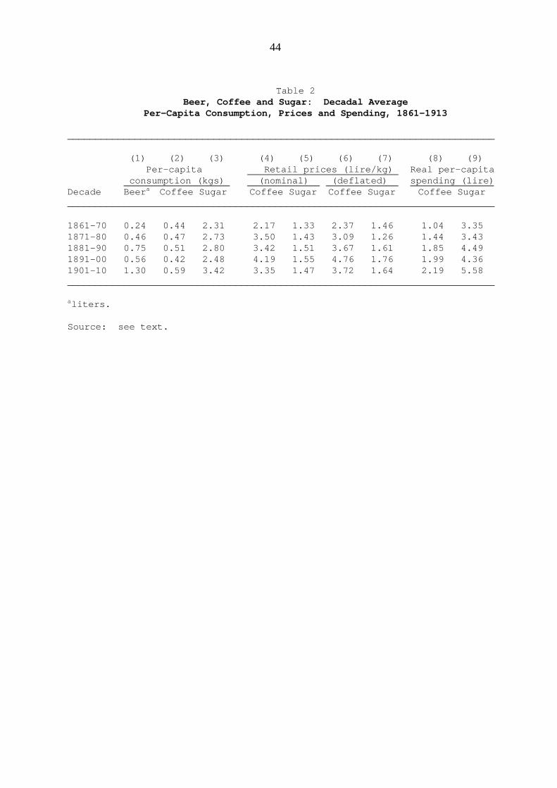
44

Table 2Beer, Coffee and Sugar: Decadal Average

Per-Capita Consumption, Prices and Spending, 1861-1913

____________________________________________________________________________

(1) (2) (3) (4) (5) (6) (7) (8) (9) Per-capita Retail prices (lire/kg) Real per-capita consumption (kgs) (nominal) (deflated) spending (lire)Decade Beera Coffee Sugar Coffee Sugar Coffee Sugar Coffee Sugar____________________________________________________________________________

1861-70 0.24 0.44 2.31 2.17 1.33 2.37 1.46 1.04 3.351871-80 0.46 0.47 2.73 3.50 1.43 3.09 1.26 1.44 3.431881-90 0.75 0.51 2.80 3.42 1.51 3.67 1.61 1.85 4.491891-00 0.56 0.42 2.48 4.19 1.55 4.76 1.76 1.99 4.361901-10 1.30 0.59 3.42 3.35 1.47 3.72 1.64 2.19 5.58____________________________________________________________________________

aliters.

Source: see text.

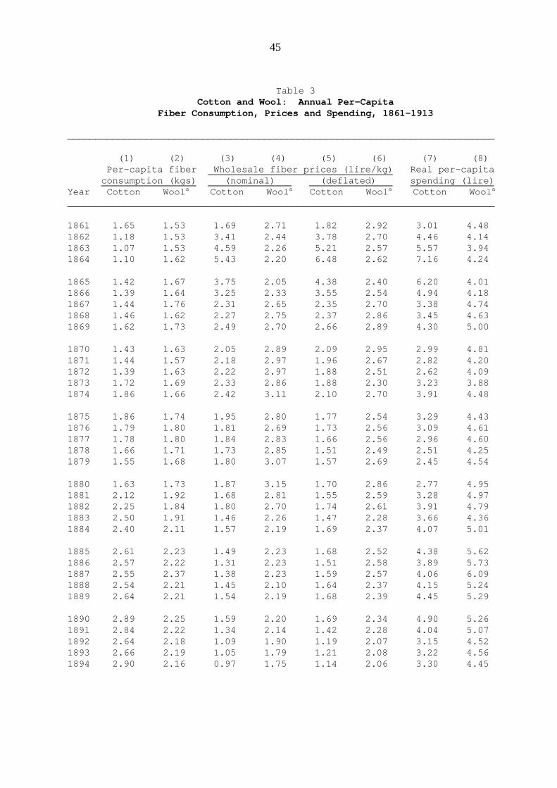
45

Table 3Cotton and Wool: Annual Per-Capita

Fiber Consumption, Prices and Spending, 1861-1913

____________________________________________________________________________

(1) (2) (3) (4) (5) (6) (7) (8) Per-capita fiber Wholesale fiber prices (lire/kg) Real per-capita consumption (kgs) (nominal) (deflated) spending (lire)Year Cotton Woola Cotton Woola Cotton Woola Cotton Woola____________________________________________________________________________ 1861 1.65 1.53 1.69 2.71 1.82 2.92 3.01 4.481862 1.18 1.53 3.41 2.44 3.78 2.70 4.46 4.141863 1.07 1.53 4.59 2.26 5.21 2.57 5.57 3.941864 1.10 1.62 5.43 2.20 6.48 2.62 7.16 4.24 1865 1.42 1.67 3.75 2.05 4.38 2.40 6.20 4.011866 1.39 1.64 3.25 2.33 3.55 2.54 4.94 4.181867 1.44 1.76 2.31 2.65 2.35 2.70 3.38 4.741868 1.46 1.62 2.27 2.75 2.37 2.86 3.45 4.631869 1.62 1.73 2.49 2.70 2.66 2.89 4.30 5.00 1870 1.43 1.63 2.05 2.89 2.09 2.95 2.99 4.811871 1.44 1.57 2.18 2.97 1.96 2.67 2.82 4.201872 1.39 1.63 2.22 2.97 1.88 2.51 2.62 4.091873 1.72 1.69 2.33 2.86 1.88 2.30 3.23 3.881874 1.86 1.66 2.42 3.11 2.10 2.70 3.91 4.48 1875 1.86 1.74 1.95 2.80 1.77 2.54 3.29 4.431876 1.79 1.80 1.81 2.69 1.73 2.56 3.09 4.611877 1.78 1.80 1.84 2.83 1.66 2.56 2.96 4.601878 1.66 1.71 1.73 2.85 1.51 2.49 2.51 4.251879 1.55 1.68 1.80 3.07 1.57 2.69 2.45 4.54 1880 1.63 1.73 1.87 3.15 1.70 2.86 2.77 4.951881 2.12 1.92 1.68 2.81 1.55 2.59 3.28 4.971882 2.25 1.84 1.80 2.70 1.74 2.61 3.91 4.791883 2.50 1.91 1.46 2.26 1.47 2.28 3.66 4.361884 2.40 2.11 1.57 2.19 1.69 2.37 4.07 5.01 1885 2.61 2.23 1.49 2.23 1.68 2.52 4.38 5.621886 2.57 2.22 1.31 2.23 1.51 2.58 3.89 5.731887 2.55 2.37 1.38 2.23 1.59 2.57 4.06 6.091888 2.54 2.21 1.45 2.10 1.64 2.37 4.15 5.241889 2.64 2.21 1.54 2.19 1.68 2.39 4.45 5.29 1890 2.89 2.25 1.59 2.20 1.69 2.34 4.90 5.261891 2.84 2.22 1.34 2.14 1.42 2.28 4.04 5.071892 2.64 2.18 1.09 1.90 1.19 2.07 3.15 4.521893 2.66 2.19 1.05 1.79 1.21 2.08 3.22 4.561894 2.90 2.16 0.97 1.75 1.14 2.06 3.30 4.45

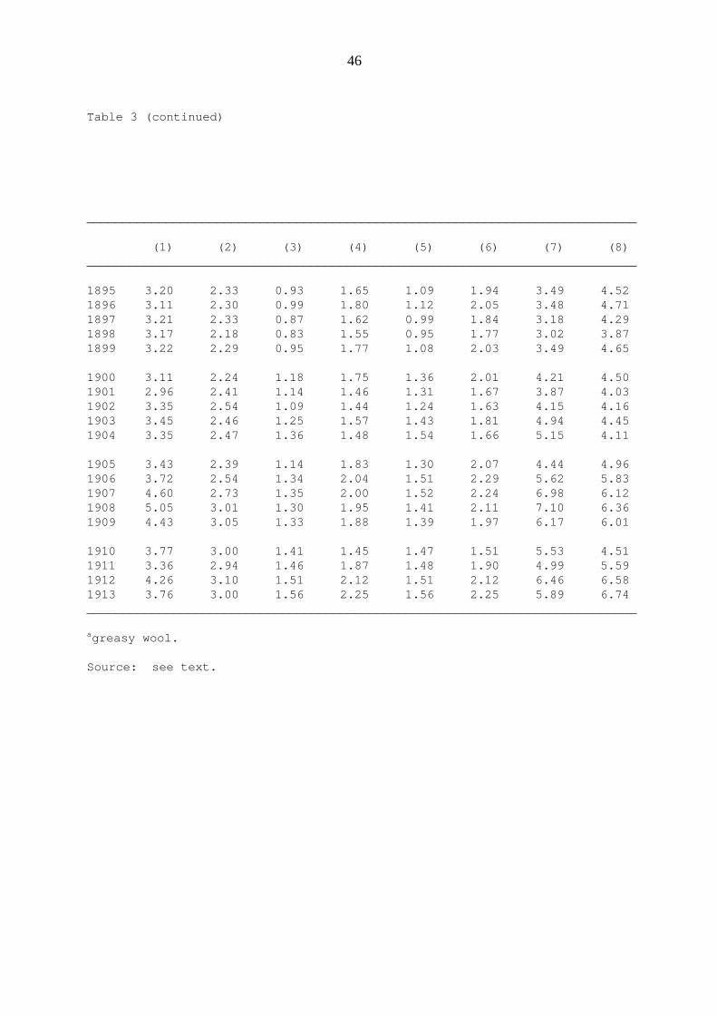
46

Table 3 (continued)

____________________________________________________________________________

(1) (2) (3) (4) (5) (6) (7) (8)____________________________________________________________________________

1895 3.20 2.33 0.93 1.65 1.09 1.94 3.49 4.521896 3.11 2.30 0.99 1.80 1.12 2.05 3.48 4.711897 3.21 2.33 0.87 1.62 0.99 1.84 3.18 4.291898 3.17 2.18 0.83 1.55 0.95 1.77 3.02 3.871899 3.22 2.29 0.95 1.77 1.08 2.03 3.49 4.65 1900 3.11 2.24 1.18 1.75 1.36 2.01 4.21 4.501901 2.96 2.41 1.14 1.46 1.31 1.67 3.87 4.031902 3.35 2.54 1.09 1.44 1.24 1.63 4.15 4.161903 3.45 2.46 1.25 1.57 1.43 1.81 4.94 4.451904 3.35 2.47 1.36 1.48 1.54 1.66 5.15 4.11 1905 3.43 2.39 1.14 1.83 1.30 2.07 4.44 4.961906 3.72 2.54 1.34 2.04 1.51 2.29 5.62 5.831907 4.60 2.73 1.35 2.00 1.52 2.24 6.98 6.121908 5.05 3.01 1.30 1.95 1.41 2.11 7.10 6.361909 4.43 3.05 1.33 1.88 1.39 1.97 6.17 6.01 1910 3.77 3.00 1.41 1.45 1.47 1.51 5.53 4.511911 3.36 2.94 1.46 1.87 1.48 1.90 4.99 5.591912 4.26 3.10 1.51 2.12 1.51 2.12 6.46 6.581913 3.76 3.00 1.56 2.25 1.56 2.25 5.89 6.74____________________________________________________________________________

agreasy wool.

Source: see text.

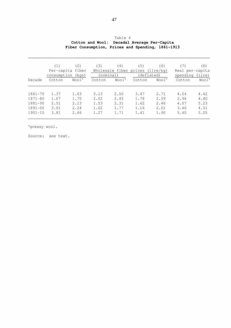
47

Table 4Cotton and Wool: Decadal Average Per-Capita

Fiber Consumption, Prices and Spending, 1861-1913

______________________________________________________________________________

(1) (2) (3) (4) (5) (6) (7) (8) Per-capita fiber Wholesale fiber prices (lire/kg) Real per-capita consumption (kgs) (nominal) (deflated) spending (lire)Decade Cotton Woola Cotton Woola Cotton Woola Cotton Woola______________________________________________________________________________

1861-70 1.37 1.63 3.13 2.50 3.47 2.71 4.54 4.421871-80 1.67 1.70 2.02 2.93 1.78 2.59 2.96 4.401881-90 2.51 2.13 1.53 2.31 1.62 2.46 4.07 5.231891-00 3.01 2.24 1.02 1.77 1.16 2.01 3.46 4.511901-10 3.81 2.66 1.27 1.71 1.41 1.90 5.40 5.05______________________________________________________________________________

agreasy wool.

Source: see text.

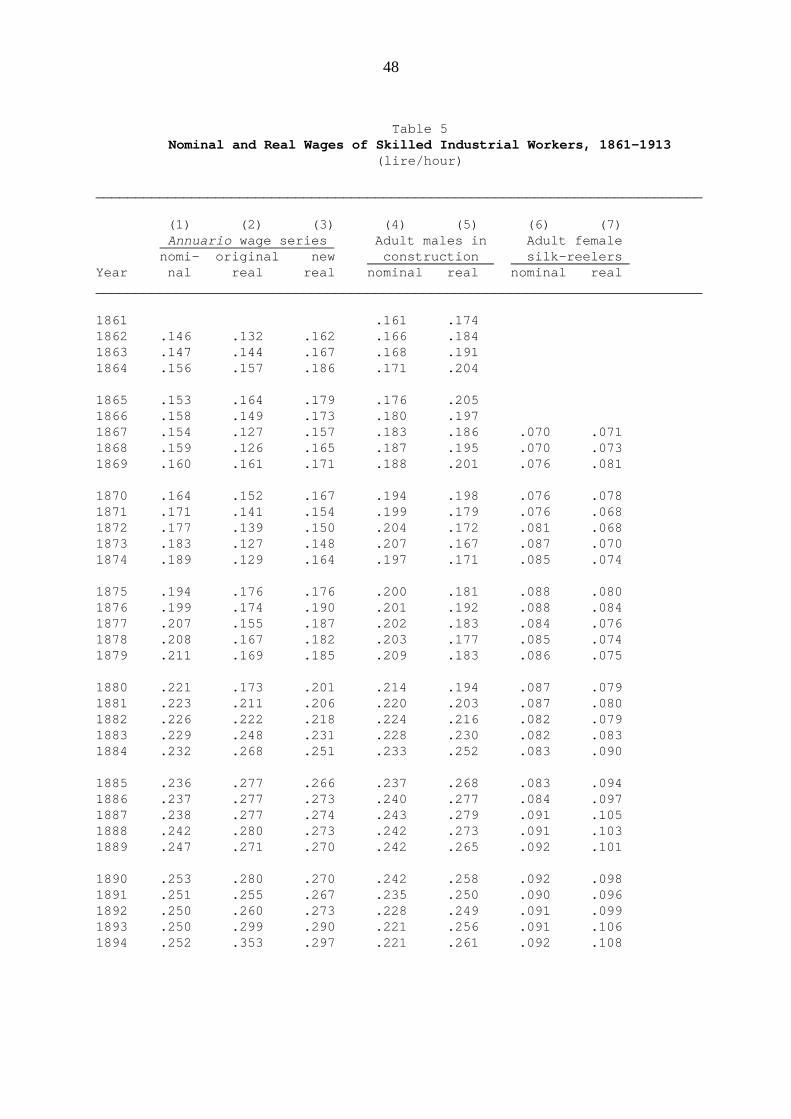
48

Table 5Nominal and Real Wages of Skilled Industrial Workers, 1861-1913

(lire/hour)

____________________________________________________________________________

(1) (2) (3) (4) (5) (6) (7) Annuario wage series Adult males in Adult female nomi- original new construction silk-reelers Year nal real real nominal real nominal real ____________________________________________________________________________ 1861 .161 .174 1862 .146 .132 .162 .166 .1841863 .147 .144 .167 .168 .1911864 .156 .157 .186 .171 .204 1865 .153 .164 .179 .176 .2051866 .158 .149 .173 .180 .1971867 .154 .127 .157 .183 .186 .070 .0711868 .159 .126 .165 .187 .195 .070 .0731869 .160 .161 .171 .188 .201 .076 .081 1870 .164 .152 .167 .194 .198 .076 .0781871 .171 .141 .154 .199 .179 .076 .0681872 .177 .139 .150 .204 .172 .081 .0681873 .183 .127 .148 .207 .167 .087 .0701874 .189 .129 .164 .197 .171 .085 .074 1875 .194 .176 .176 .200 .181 .088 .0801876 .199 .174 .190 .201 .192 .088 .0841877 .207 .155 .187 .202 .183 .084 .0761878 .208 .167 .182 .203 .177 .085 .0741879 .211 .169 .185 .209 .183 .086 .075 1880 .221 .173 .201 .214 .194 .087 .0791881 .223 .211 .206 .220 .203 .087 .0801882 .226 .222 .218 .224 .216 .082 .0791883 .229 .248 .231 .228 .230 .082 .0831884 .232 .268 .251 .233 .252 .083 .090 1885 .236 .277 .266 .237 .268 .083 .0941886 .237 .277 .273 .240 .277 .084 .0971887 .238 .277 .274 .243 .279 .091 .1051888 .242 .280 .273 .242 .273 .091 .1031889 .247 .271 .270 .242 .265 .092 .101 1890 .253 .280 .270 .242 .258 .092 .0981891 .251 .255 .267 .235 .250 .090 .0961892 .250 .260 .273 .228 .249 .091 .0991893 .250 .299 .290 .221 .256 .091 .1061894 .252 .353 .297 .221 .261 .092 .108

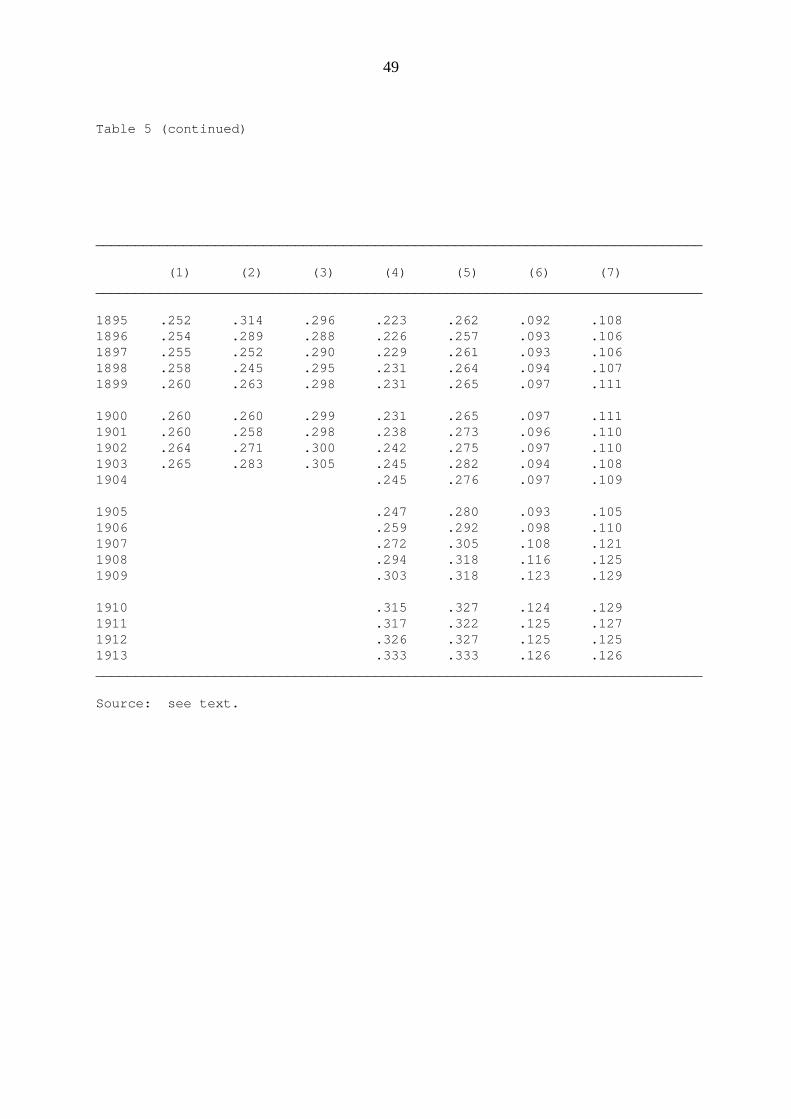
49

Table 5 (continued)

____________________________________________________________________________

(1) (2) (3) (4) (5) (6) (7)____________________________________________________________________________

1895 .252 .314 .296 .223 .262 .092 .1081896 .254 .289 .288 .226 .257 .093 .1061897 .255 .252 .290 .229 .261 .093 .1061898 .258 .245 .295 .231 .264 .094 .1071899 .260 .263 .298 .231 .265 .097 .111 1900 .260 .260 .299 .231 .265 .097 .1111901 .260 .258 .298 .238 .273 .096 .1101902 .264 .271 .300 .242 .275 .097 .1101903 .265 .283 .305 .245 .282 .094 .1081904 .245 .276 .097 .109 1905 .247 .280 .093 .1051906 .259 .292 .098 .1101907 .272 .305 .108 .1211908 .294 .318 .116 .1251909 .303 .318 .123 .129 1910 .315 .327 .124 .1291911 .317 .322 .125 .1271912 .326 .327 .125 .1251913 .333 .333 .126 .126____________________________________________________________________________

Source: see text.

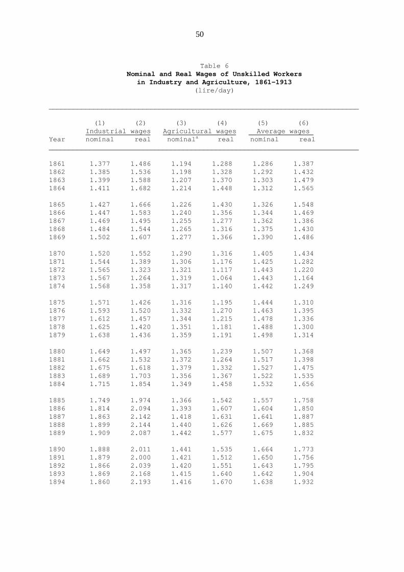
50

Table 6Nominal and Real Wages of Unskilled Workers

in Industry and Agriculture, 1861-1913(lire/day)

____________________________________________________________________________

(1) (2) (3) (4) (5) (6) Industrial wages Agricultural wages Average wages Year nominal real nominala real nominal real ____________________________________________________________________________ 1861 1.377 1.486 1.194 1.288 1.286 1.3871862 1.385 1.536 1.198 1.328 1.292 1.4321863 1.399 1.588 1.207 1.370 1.303 1.4791864 1.411 1.682 1.214 1.448 1.312 1.565 1865 1.427 1.666 1.226 1.430 1.326 1.5481866 1.447 1.583 1.240 1.356 1.344 1.4691867 1.469 1.495 1.255 1.277 1.362 1.3861868 1.484 1.544 1.265 1.316 1.375 1.4301869 1.502 1.607 1.277 1.366 1.390 1.486 1870 1.520 1.552 1.290 1.316 1.405 1.4341871 1.544 1.389 1.306 1.176 1.425 1.2821872 1.565 1.323 1.321 1.117 1.443 1.2201873 1.567 1.264 1.319 1.064 1.443 1.1641874 1.568 1.358 1.317 1.140 1.442 1.249 1875 1.571 1.426 1.316 1.195 1.444 1.3101876 1.593 1.520 1.332 1.270 1.463 1.3951877 1.612 1.457 1.344 1.215 1.478 1.3361878 1.625 1.420 1.351 1.181 1.488 1.3001879 1.638 1.436 1.359 1.191 1.498 1.314 1880 1.649 1.497 1.365 1.239 1.507 1.3681881 1.662 1.532 1.372 1.264 1.517 1.3981882 1.675 1.618 1.379 1.332 1.527 1.4751883 1.689 1.703 1.356 1.367 1.522 1.5351884 1.715 1.854 1.349 1.458 1.532 1.656 1885 1.749 1.974 1.366 1.542 1.557 1.7581886 1.814 2.094 1.393 1.607 1.604 1.8501887 1.863 2.142 1.418 1.631 1.641 1.8871888 1.899 2.144 1.440 1.626 1.669 1.8851889 1.909 2.087 1.442 1.577 1.675 1.832 1890 1.888 2.011 1.441 1.535 1.664 1.7731891 1.879 2.000 1.421 1.512 1.650 1.7561892 1.866 2.039 1.420 1.551 1.643 1.7951893 1.869 2.168 1.415 1.640 1.642 1.9041894 1.860 2.193 1.416 1.670 1.638 1.932

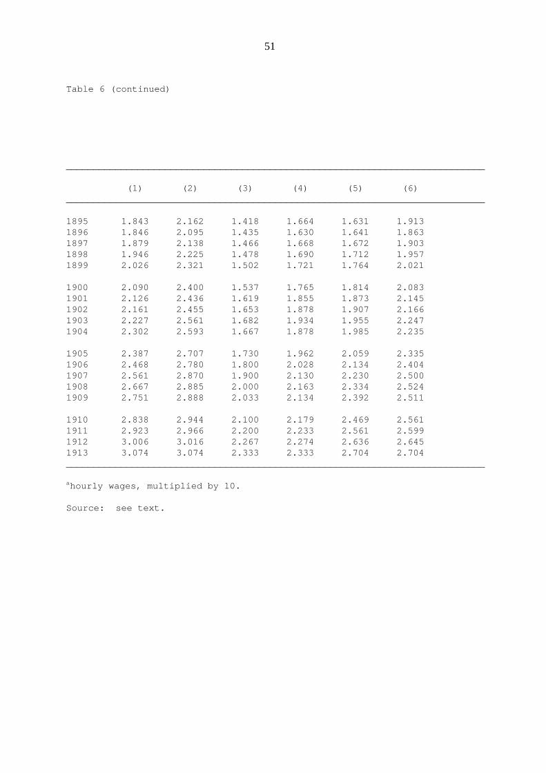
51

Table 6 (continued)

____________________________________________________________________________

(1) (2) (3) (4) (5) (6)____________________________________________________________________________

1895 1.843 2.162 1.418 1.664 1.631 1.9131896 1.846 2.095 1.435 1.630 1.641 1.8631897 1.879 2.138 1.466 1.668 1.672 1.9031898 1.946 2.225 1.478 1.690 1.712 1.9571899 2.026 2.321 1.502 1.721 1.764 2.021 1900 2.090 2.400 1.537 1.765 1.814 2.0831901 2.126 2.436 1.619 1.855 1.873 2.1451902 2.161 2.455 1.653 1.878 1.907 2.1661903 2.227 2.561 1.682 1.934 1.955 2.2471904 2.302 2.593 1.667 1.878 1.985 2.235 1905 2.387 2.707 1.730 1.962 2.059 2.3351906 2.468 2.780 1.800 2.028 2.134 2.4041907 2.561 2.870 1.900 2.130 2.230 2.5001908 2.667 2.885 2.000 2.163 2.334 2.5241909 2.751 2.888 2.033 2.134 2.392 2.511 1910 2.838 2.944 2.100 2.179 2.469 2.5611911 2.923 2.966 2.200 2.233 2.561 2.5991912 3.006 3.016 2.267 2.274 2.636 2.6451913 3.074 3.074 2.333 2.333 2.704 2.704____________________________________________________________________________

ahourly wages, multiplied by 10.

Source: see text.

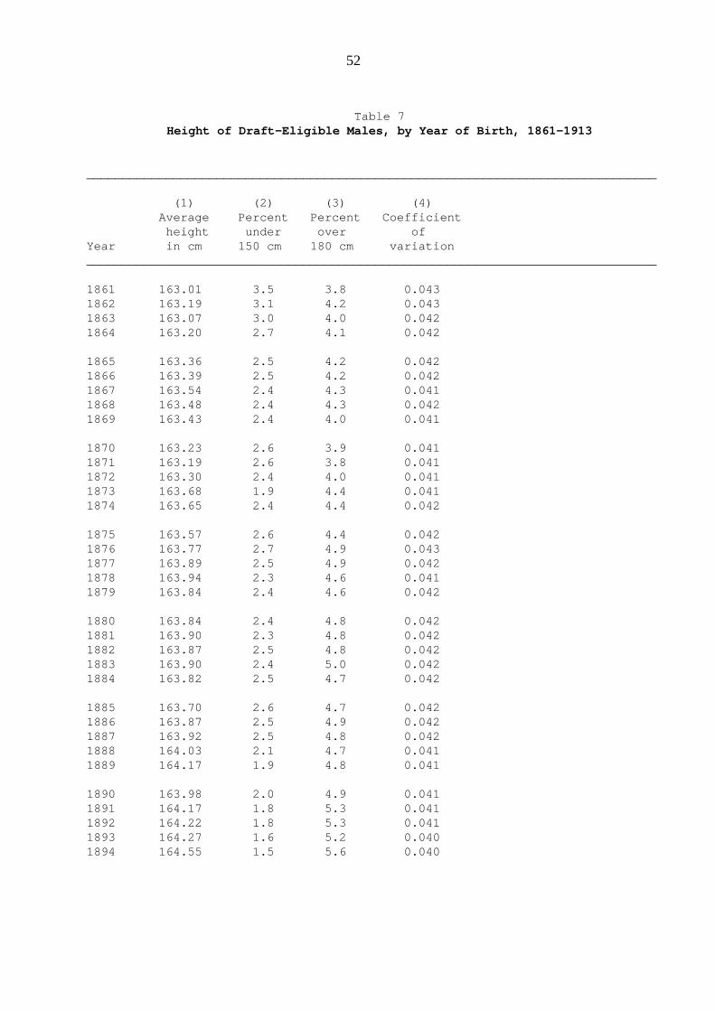
52

Table 7Height of Draft-Eligible Males, by Year of Birth, 1861-1913

_______________________________________________________________________________

(1) (2) (3) (4) Average Percent Percent Coefficient height under over ofYear in cm 150 cm 180 cm variation_______________________________________________________________________________ 1861 163.01 3.5 3.8 0.043 1862 163.19 3.1 4.2 0.0431863 163.07 3.0 4.0 0.0421864 163.20 2.7 4.1 0.042 1865 163.36 2.5 4.2 0.0421866 163.39 2.5 4.2 0.0421867 163.54 2.4 4.3 0.0411868 163.48 2.4 4.3 0.0421869 163.43 2.4 4.0 0.041 1870 163.23 2.6 3.9 0.0411871 163.19 2.6 3.8 0.0411872 163.30 2.4 4.0 0.0411873 163.68 1.9 4.4 0.0411874 163.65 2.4 4.4 0.042 1875 163.57 2.6 4.4 0.0421876 163.77 2.7 4.9 0.0431877 163.89 2.5 4.9 0.0421878 163.94 2.3 4.6 0.0411879 163.84 2.4 4.6 0.042 1880 163.84 2.4 4.8 0.0421881 163.90 2.3 4.8 0.0421882 163.87 2.5 4.8 0.0421883 163.90 2.4 5.0 0.0421884 163.82 2.5 4.7 0.042 1885 163.70 2.6 4.7 0.0421886 163.87 2.5 4.9 0.0421887 163.92 2.5 4.8 0.0421888 164.03 2.1 4.7 0.0411889 164.17 1.9 4.8 0.041 1890 163.98 2.0 4.9 0.0411891 164.17 1.8 5.3 0.0411892 164.22 1.8 5.3 0.0411893 164.27 1.6 5.2 0.0401894 164.55 1.5 5.6 0.040

53

Table 7 (continued)

_______________________________________________________________________________

(1) (2) (3) (4) _______________________________________________________________________________

1895 164.24 1.8 5.3 0.0411896 164.44 1.8 5.7 0.0411897 164.08 2.1 5.3 0.0421898 163.73 2.6 4.9 0.0431899 162.88 3.8 3.9 0.044 1900 162.53 5.2 4.1 0.0461901 164.54 1.8 6.2 0.0421902 164.56 1.7 5.9 0.0421903 164.89 1.7 6.4 0.0421904 165.08 1.4 6.8 0.041 1905 165.05 1.2 6.6 0.0411906 165.18 1.2 6.6 0.0411907 165.22 1.2 7.0 0.0411908 165.37 1.1 7.1 0.0411909 165.39 1.1 7.2 0.041 1910 165.50 1.0 7.5 0.0411911 166.10 0.7 8.7 0.0401912 166.12 0.8 8.8 0.0401913 166.23 0.8 9.2 0.041_______________________________________________________________________________

Source: see text.

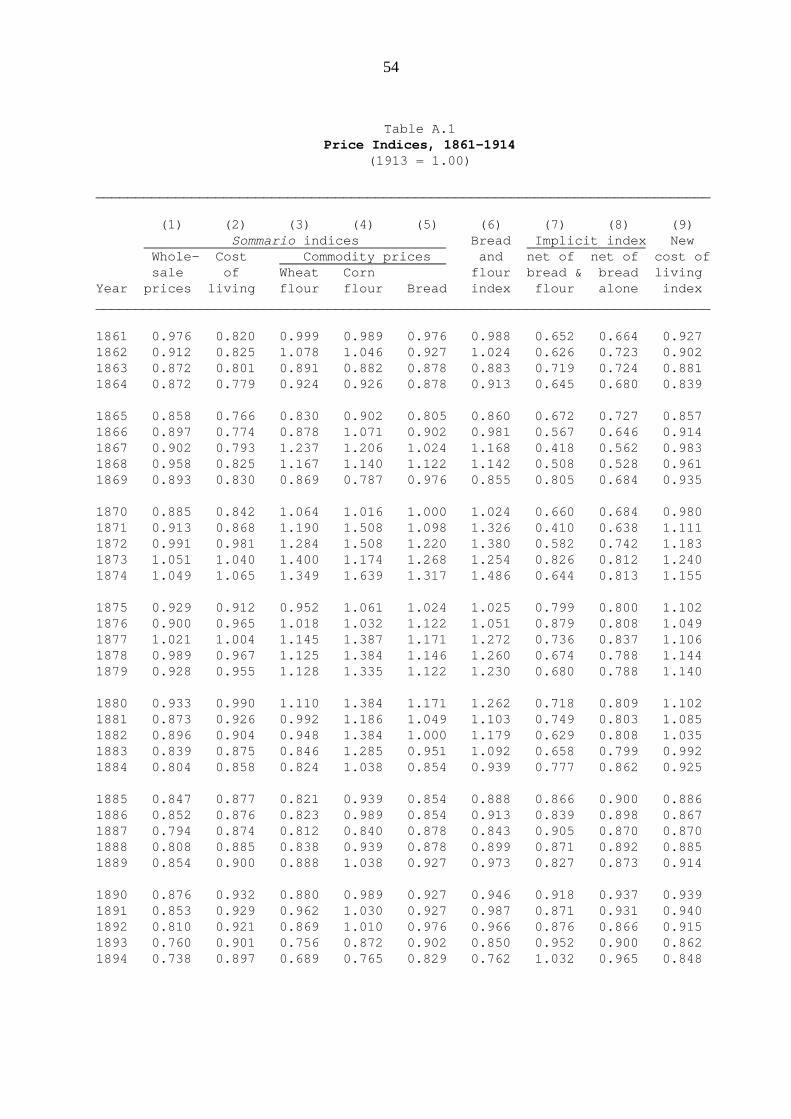
54

Table A.1Price Indices, 1861-1914

(1913 = 1.00)

_____________________________________________________________________________

(1) (2) (3) (4) (5) (6) (7) (8) (9) Sommario indices Bread Implicit index New Whole- Cost Commodity prices and net of net of cost of sale of Wheat Corn flour bread & bread livingYear prices living flour flour Bread index flour alone index_____________________________________________________________________________

1861 0.976 0.820 0.999 0.989 0.976 0.988 0.652 0.664 0.9271862 0.912 0.825 1.078 1.046 0.927 1.024 0.626 0.723 0.9021863 0.872 0.801 0.891 0.882 0.878 0.883 0.719 0.724 0.8811864 0.872 0.779 0.924 0.926 0.878 0.913 0.645 0.680 0.839

1865 0.858 0.766 0.830 0.902 0.805 0.860 0.672 0.727 0.8571866 0.897 0.774 0.878 1.071 0.902 0.981 0.567 0.646 0.9141867 0.902 0.793 1.237 1.206 1.024 1.168 0.418 0.562 0.9831868 0.958 0.825 1.167 1.140 1.122 1.142 0.508 0.528 0.9611869 0.893 0.830 0.869 0.787 0.976 0.855 0.805 0.684 0.935

1870 0.885 0.842 1.064 1.016 1.000 1.024 0.660 0.684 0.9801871 0.913 0.868 1.190 1.508 1.098 1.326 0.410 0.638 1.1111872 0.991 0.981 1.284 1.508 1.220 1.380 0.582 0.742 1.1831873 1.051 1.040 1.400 1.174 1.268 1.254 0.826 0.812 1.2401874 1.049 1.065 1.349 1.639 1.317 1.486 0.644 0.813 1.155

1875 0.929 0.912 0.952 1.061 1.024 1.025 0.799 0.800 1.1021876 0.900 0.965 1.018 1.032 1.122 1.051 0.879 0.808 1.0491877 1.021 1.004 1.145 1.387 1.171 1.272 0.736 0.837 1.1061878 0.989 0.967 1.125 1.384 1.146 1.260 0.674 0.788 1.1441879 0.928 0.955 1.128 1.335 1.122 1.230 0.680 0.788 1.140

1880 0.933 0.990 1.110 1.384 1.171 1.262 0.718 0.809 1.1021881 0.873 0.926 0.992 1.186 1.049 1.103 0.749 0.803 1.0851882 0.896 0.904 0.948 1.384 1.000 1.179 0.629 0.808 1.0351883 0.839 0.875 0.846 1.285 0.951 1.092 0.658 0.799 0.9921884 0.804 0.858 0.824 1.038 0.854 0.939 0.777 0.862 0.925

1885 0.847 0.877 0.821 0.939 0.854 0.888 0.866 0.900 0.8861886 0.852 0.876 0.823 0.989 0.854 0.913 0.839 0.898 0.8671887 0.794 0.874 0.812 0.840 0.878 0.843 0.905 0.870 0.8701888 0.808 0.885 0.838 0.939 0.878 0.899 0.871 0.892 0.8851889 0.854 0.900 0.888 1.038 0.927 0.973 0.827 0.873 0.914

1890 0.876 0.932 0.880 0.989 0.927 0.946 0.918 0.937 0.9391891 0.853 0.929 0.962 1.030 0.927 0.987 0.871 0.931 0.9401892 0.810 0.921 0.869 1.010 0.976 0.966 0.876 0.866 0.9151893 0.760 0.901 0.756 0.872 0.902 0.850 0.952 0.900 0.8621894 0.738 0.897 0.689 0.765 0.829 0.762 1.032 0.965 0.848

55

Table A.1 (continued)

_____________________________________________________________________________

(1) (2) (3) (4) (5) (6) (7) (8) (9)_____________________________________________________________________________

1895 0.776 0.892 0.788 1.009 0.854 0.915 0.869 0.930 0.8521896 0.782 0.888 0.856 0.910 0.829 0.876 0.900 0.947 0.8811897 0.766 0.886 0.951 0.893 0.854 0.898 0.874 0.918 0.8791898 0.787 0.892 1.025 0.835 0.927 0.905 0.879 0.857 0.8751899 0.808 0.878 0.918 0.804 0.927 0.863 0.893 0.829 0.873

1900 0.845 0.882 0.931 0.855 0.927 0.892 0.872 0.837 0.8711901 0.841 0.883 0.949 0.875 0.902 0.900 0.866 0.864 0.8731902 0.813 0.877 0.911 0.851 0.878 0.873 0.881 0.876 0.8801903 0.806 0.903 0.876 0.954 0.878 0.916 0.890 0.928 0.8701904 0.770 0.914 0.858 0.830 0.829 0.837 0.991 0.999 0.888

1905 0.803 0.915 0.905 1.004 0.829 0.936 0.894 1.001 0.8821906 0.833 0.932 0.898 0.884 0.829 0.874 0.990 1.035 0.8881907 0.898 0.976 0.868 0.804 0.854 0.832 1.120 1.098 0.8921908 0.874 0.966 0.955 0.957 0.854 0.931 1.001 1.078 0.9251909 0.881 0.939 1.071 1.062 0.878 1.018 0.860 1.000 0.953

1910 0.882 0.965 0.895 1.009 0.951 0.966 0.964 0.979 0.9641911 0.953 0.989 0.970 0.969 0.976 0.971 1.007 1.002 0.9851912 1.028 0.998 1.071 1.163 0.951 1.087 0.909 1.045 0.9971913 1.000 1.000 1.000 1.000 1.000 1.000 1.000 1.000 1.0001914 .958 1.000 1.007 0.970 0.976 0.981 1.019 1.024 _____________________________________________________________________________

Source: see text.

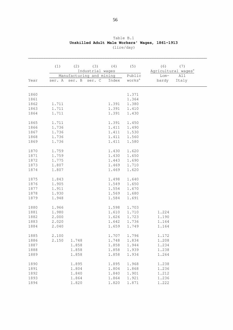
56

Table B.1Unskilled Adult Male Workers' Wages, 1861-1913

(lire/day)

____________________________________________________________________________

(1) (2) (3) (4) (5) (6) (7) Industrial wages Agricultural wagesa Manufacturing and mining Public Lom- AllYear ser. A ser. B ser. C Index worksa bardy Italy____________________________________________________________________________ 1860 1.3711861 1.3641862 1.711 1.391 1.3801863 1.711 1.391 1.4101864 1.711 1.391 1.430

1865 1.711 1.391 1.450 1866 1.736 1.411 1.490 1867 1.736 1.411 1.530 1868 1.736 1.411 1.560 1869 1.736 1.411 1.580

1870 1.759 1.430 1.620 1871 1.759 1.430 1.650 1872 1.775 1.443 1.690 1873 1.807 1.469 1.710 1874 1.807 1.469 1.620

1875 1.843 1.498 1.640 1876 1.905 1.549 1.650 1877 1.911 1.554 1.670 1878 1.930 1.569 1.680 1879 1.948 1.584 1.691

1880 1.966 1.598 1.703 1881 1.980 1.610 1.710 1.224 1882 2.000 1.626 1.723 1.190 1883 2.020 1.642 1.736 1.164 1884 2.040 1.659 1.749 1.164

1885 2.100 1.707 1.796 1.172 1886 2.150 1.748 1.748 1.834 1.208 1887 1.858 1.858 1.944 1.234 1888 1.858 1.858 1.939 1.238 1889 1.858 1.858 1.934 1.264

1890 1.895 1.895 1.968 1.238 1891 1.804 1.804 1.868 1.236 1892 1.840 1.840 1.901 1.212 1893 1.864 1.864 1.921 1.236 1894 1.820 1.820 1.871 1.222

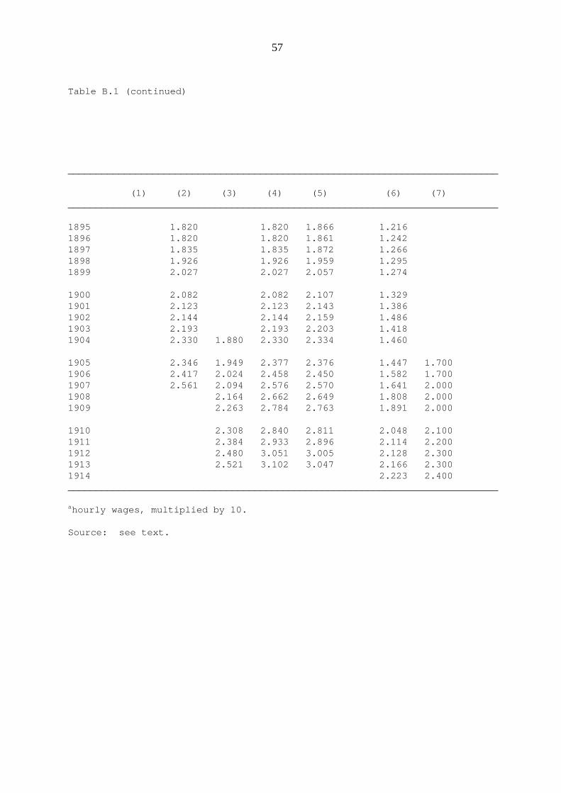
57

Table B.1 (continued)

____________________________________________________________________________

(1) (2) (3) (4) (5) (6) (7) ____________________________________________________________________________

1895 1.820 1.820 1.866 1.216 1896 1.820 1.820 1.861 1.242 1897 1.835 1.835 1.872 1.266 1898 1.926 1.926 1.959 1.295 1899 2.027 2.027 2.057 1.274

1900 2.082 2.082 2.107 1.329 1901 2.123 2.123 2.143 1.386 1902 2.144 2.144 2.159 1.486 1903 2.193 2.193 2.203 1.418 1904 2.330 1.880 2.330 2.334 1.460

1905 2.346 1.949 2.377 2.376 1.447 1.700 1906 2.417 2.024 2.458 2.450 1.582 1.700 1907 2.561 2.094 2.576 2.570 1.641 2.000 1908 2.164 2.662 2.649 1.808 2.000 1909 2.263 2.784 2.763 1.891 2.000

1910 2.308 2.840 2.811 2.048 2.100 1911 2.384 2.933 2.896 2.114 2.200 1912 2.480 3.051 3.005 2.128 2.300 1913 2.521 3.102 3.047 2.166 2.300 1914 2.223 2.400 ____________________________________________________________________________

ahourly wages, multiplied by 10.

Source: see text.

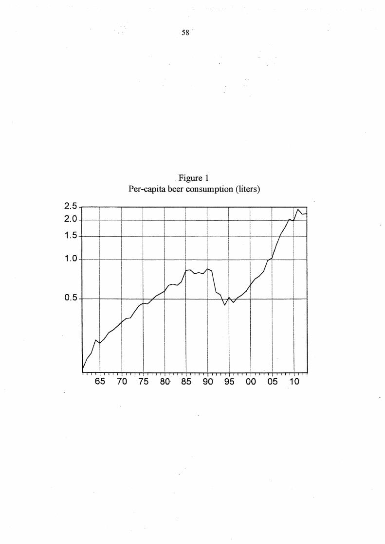
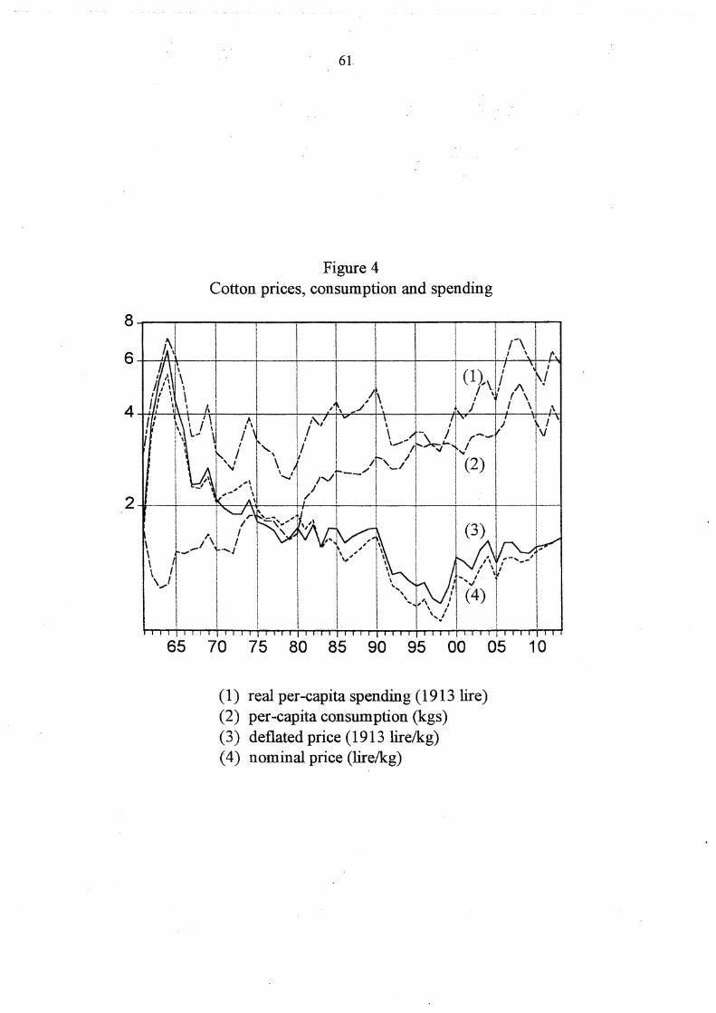
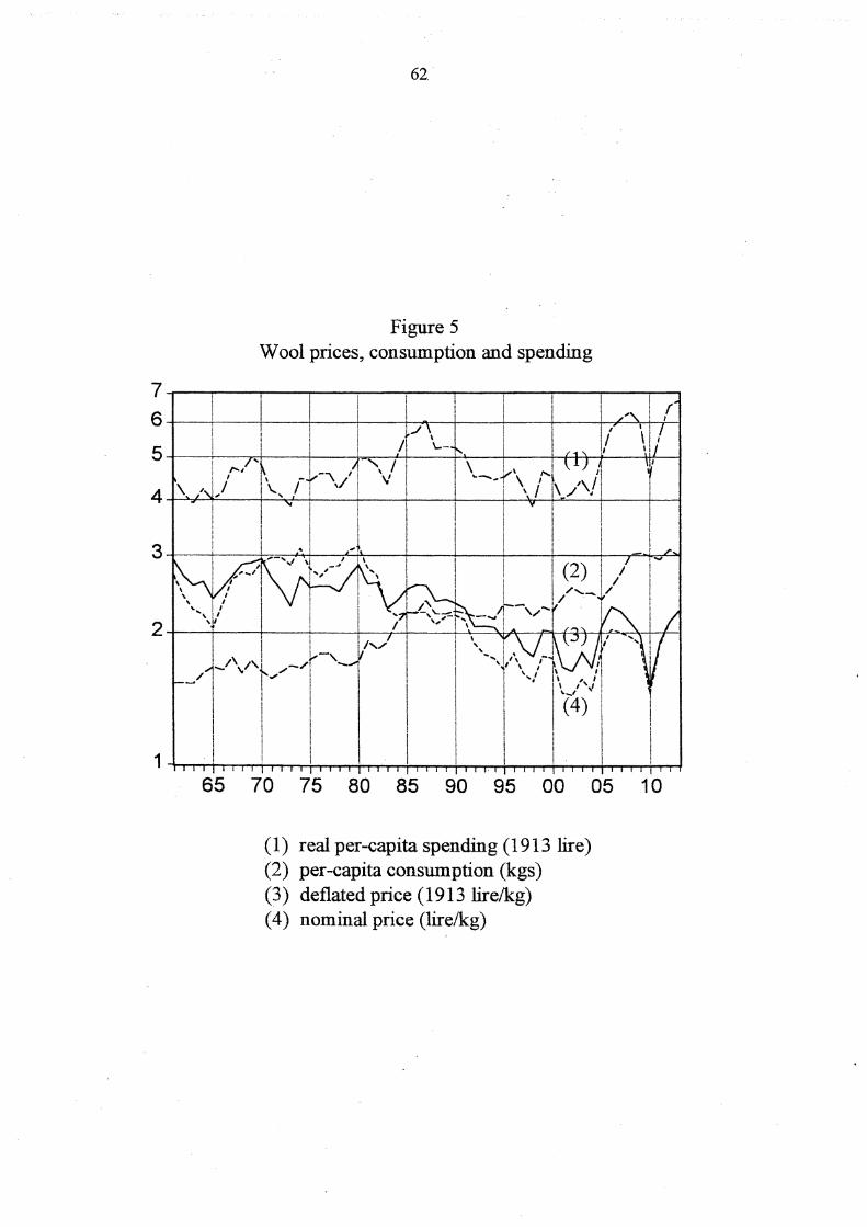
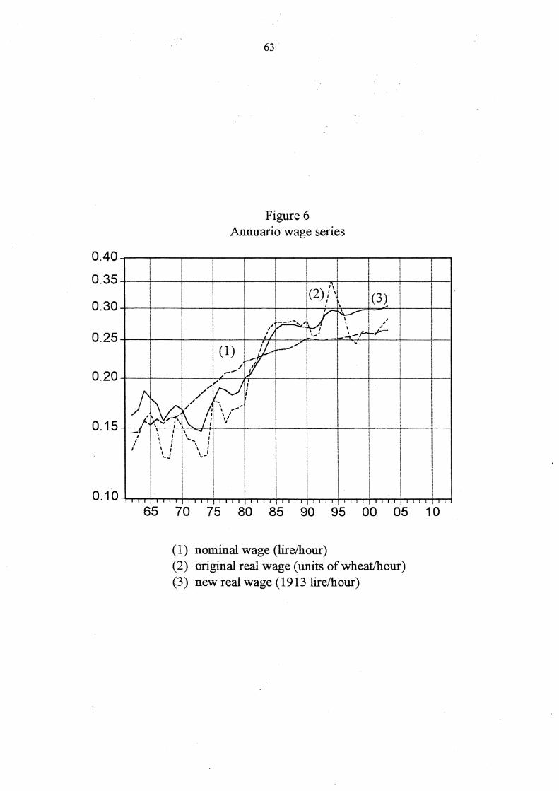
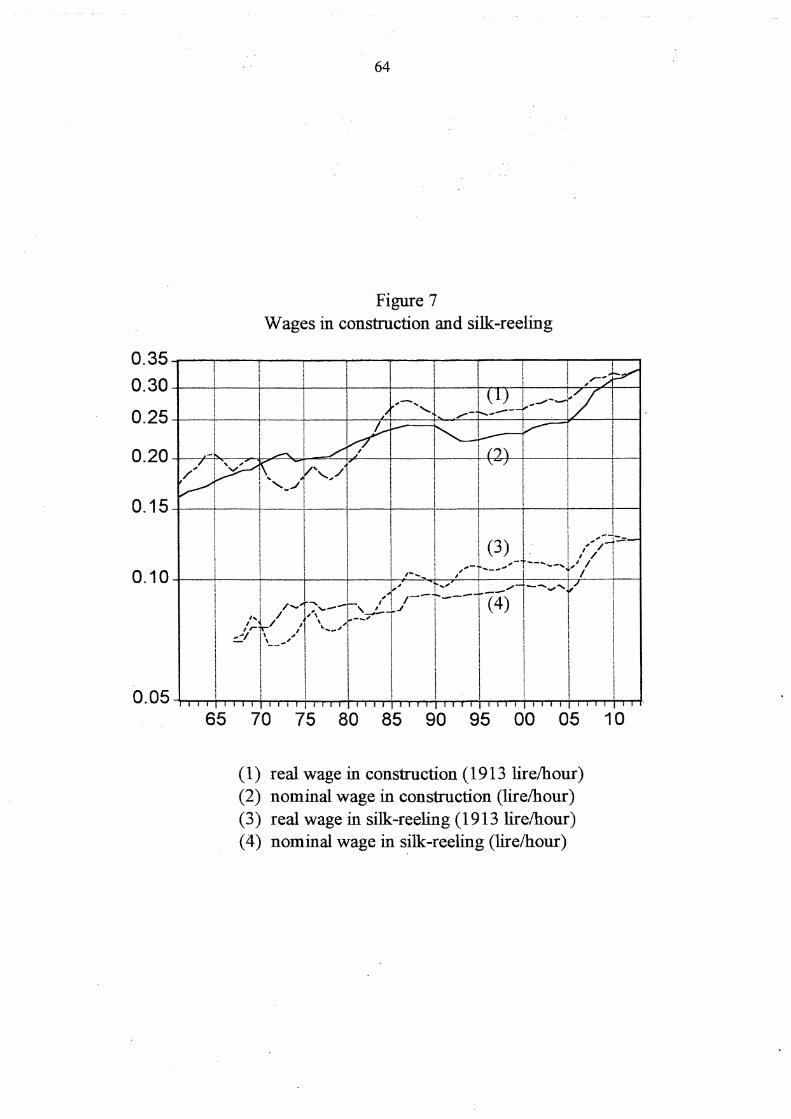
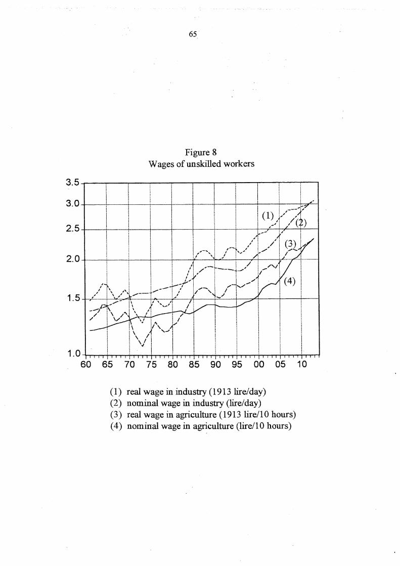
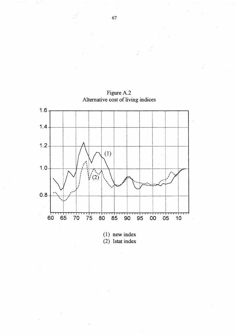
References

Albertario, P. (1931), Salari agricoli nelle zone ad economia capitalistica della BassaLombardia nel cinquantennio 1881-1930, Pavia, Istituto nazionale di economiaagraria.

Aleati, G. (1961), Le retribuzioni dei lavori edili in Milano, Pavia e nei rispettivi territoridal 1819 al 1890, Archivio economico della unificazione italiana, serie I, vol. XI, fasc.1, Torino, I.L.T.E.

Annuario: Direzione generale della statistica, Annuario statistico italiano, various years.

Arcari, P.M. (1936), Le variazioni dei salari agricoli in Italia dalla fondazione del Regno al1933, Istituto centrale di statistica, Annali di statistica, serie VI, vol. 36, Roma.

Bandettini, P.F. (1960), Le retribuzioni dei lavori edili a Firenze dal 1819 al 1890, Archivioeconomico della unificazione italiana, serie I, vol. X, fasc. 3, Torino, I.L.T.E.

Barberi, B. (1961), I consumi nel primo secolo dell’Unità d’Italia, Milano, Giuffrè.

Bollettino del lavoro: Ministero di agricoltura, industria e commercio, Bollettino dell’Ufficiodel lavoro, various years.

Castronovo, V. (1995), Storia economica d’Italia, Torino, Einaudi.

Censimento 1881: Direzione generale della statistica, Censimento della popolazione delRegno d’Italia al 31 dicembre 1881, vol. III, Roma, Tipografia Bodoniana, 1884.

Croce, B. (1967), Storia d’Italia dal 1871 al 1915, Bari, Laterza.

De Bernardi, A., ed. (1977), Questione agraria e protezionismo nella crisi economica di finesecolo, Milano, Franco Angeli.

di Rollo, F. (1965), Le retribuzioni dei lavori edili a Roma dal 1826 al 1880, Archivioeconomico della unificazione italiana, serie I, vol. XIII, fasc. 4, Torino, I.L.T.E.

Federico, G. (1982), “Per una valutazione critica delle statistiche della produzione agricolaitaliana dopo l’Unità,” Società e storia 15, pp. 87-130.

Federico, G. (1984), “Commercio dei cereali e dazio sul grano in Italia (1863-1913). Unaanalisi quantitativa,” Nuova rivista storica 68, pp. 46-108.

Federico, G. (1994), Il filo d’oro. L’industria mondiale della seta dalla restaurazione allagrande crisi, Venezia, Marsilio.

Federico, G. (2000), “Una stima del valore aggiunto dell’agricoltura italiana,” in G.M. Rey,ed., I conti economici dell’Italia. 3**. Il valore aggiunto per gli anni 1891, 1938,1951, pp. 3-112, Collana storica della Banca d’Italia, Roma-Bari, Laterza.

Felloni, G. (1963), Le retribuzioni dei lavori edili a Genova dal 1815 al 1890, Archivioeconomico della unificazione italiana, serie I, vol. XII, fasc. 3, Torino, I.L.T.E.

Fenoaltea, S. (1969), “Decollo, ciclo, e intervento dello Stato,” in A. Caracciolo, ed., Laformazione dell’Italia industriale, pp. 95-113, Bari, Laterza.

69

Fenoaltea, S. (1986), “Public Works Construction in Italy, 1861-1913,” Rivista di storiaeconomica 3, International issue, pp. 1-33.

Fenoaltea, S. (1988a), “International Resource Flows and Construction Movements in theAtlantic Economy: The Kuznets Cycle in Italy, 1861-1913,” Journal of EconomicHistory 48, pp. 605-38.

Fenoaltea, S. (1988b), “The Growth of Italy’s Silk Industry, 1861-1913: A StatisticalReconstruction,” Rivista di storia economica 5, pp. 275-318.

Fenoaltea, S. (1993), “Politica doganale, sviluppo industriale, emigrazione: verso unariconsiderazione del dazio sul grano,” Rivista di storia economica 10, pp. 65-77.

Fenoaltea, S. (1998), “Lo sviluppo economico dell’Italia nel lungo periodo: riflessioni su trefallimenti,” in P.L. Ciocca and G. Toniolo, eds., Storia economica d’Italia, vol. 1,Interpretazioni, pp. 3-41, Milano-Roma-Bari, Cariplo-Laterza.

Fenoaltea, S. (2000), “The Growth of Italy’s Wool Industry, 1861-1913: A StatisticalReconstruction,” Rivista di storia economica 16, pp. 119-45.

Fenoaltea, S. (2001), “The Growth of Italy’s Cotton Industry, 1861-1913: A StatisticalReconstruction,” Rivista di storia economica 17, pp. 139-71.

Fenoaltea, S. (2002), “Textile Production in Italy, 1861-1913,” Rivista di storia economica18, pp. 3-40.

Geisser, A., and E. Magrini (1904), Contribuzione alla storia e statistica dei salariindustriali in Italia nella seconda metà del secolo XIX, Torino, Roux e Viarengo.

Gerschenkron, A. (1962), Economic Backwardness in Historical Perspective, Cambridge,Mass., Belknap Press.

Luzzatto, G. (1968), L’economia italiana dal 1861 al 1894, Torino, Einaudi.

Mercedi: Direzione generale della statistica, Saggio di statistica delle mercedi. Mercedipagate agli operai degli stabilimenti meccanici e metallurgici e dei cantieri navali.Notizie sommarie sulle mercedi pagate in altre industrie. Annali di statistica, serie IV,vol. 26, Roma, 1888.

Mitchell, B.R., and P. Deane (1962), Abstract of British Historical Statistics, Cambridge,Cambridge University Press.

Postan, M.M. (1939), “The Fifteenth Century,” Economic History Review 9, pp. 160-67.

Rilevazioni statistiche: Istituto centrale di statistica (Istat), Le rilevazioni statistiche in Italiadal 1861 al 1956. Statistiche dell’attività produttiva. Statistiche economiche generali.Annali di statistica, serie VIII, vol. 7, Roma, 1958.

Romeo, R. (1963), Risorgimento e capitalismo, 2d ed., Bari, Laterza.

Salari 1862-78: Direzione generale della statistica, Salari. Prezzi medii di un’ora di lavorodegli operai addetti alle opere di muratura ed ai trasporti di terra e mercedi mediegiornaliere degli operai addetti alle miniere (1862-1878), Roma, n.d.

70

Salari 1906: Ufficio del lavoro, Salari e orari nei lavori edilizi, stradali, idraulici e dibonifica (anno 1906), Roma, 1907.

Sensini, G. (1904), Le variazioni dello stato economico dell’Italia nell’ultimo trentennio delsecolo XIX, Roma, Loescher.

Sommario: Istituto centrale di statistica (Istat), Sommario di statistiche storiche italiane,1861-1955, Roma, 1958.

Toniolo, G. (1988), Storia economica dell’Italia liberale, 1850-1918, Bologna, Il Mulino.

Wilcox, W.F., ed. (1929), International migrations, vol. 1, Statistics, New York, NationalBureau of Economic Research.

Zamagni, V. (1990), Dalla periferia al centro: la seconda rinascita economica dell’Italia,1861-1981, Bologna, Il Mulino.

PREVIOUSLY PUBLISHED “QUADERNI” (*)

1 — STEFANO FENOALTEA, La crescita industriale delle regioni d’Italia dall’Unità alla Gran-de Guerra: una prima stima per gli anni censuari, June 2001.

2 — ISABELLA CERIONI, La Banca d’Italia e il Consorzio Siderurgico. Fonti per la storia dellasiderurgia in età giolittiana nelle carte dell’Archivio della Banca d’Italia, June 2001.

3 — RENATA MARTANO, La Banca d’Italia e i provvedimenti a favore dell’industria serica trail 1918 e il 1922, nelle carte dell’Archivio della Banca d’Italia, June 2001.

4 — ANNA RITA RIGANO, La Banca d’Italia e il progetto ENSI. Fonti per la storia dello svilup-po energetico italiano degli anni cinquanta nelle carte dell’Archivio della Banca d’Ita-lia, June 2002.

(*) The Quaderni are available on the Internet at www.bancaditalia.it.