Embed Size (px)
DESCRIPTION
Detailed tutorial
Citation preview
7/18/2019 PVTsim Tutorial Calsep
http://slidepdf.com/reader/full/pvtsim-tutorial-calsep 1/140
Method Documentation
PVTsim 13
CALSEP
7/18/2019 PVTsim Tutorial Calsep
http://slidepdf.com/reader/full/pvtsim-tutorial-calsep 2/140
ContentsIntroduction 5
Introduction .............................................................. ................................................................ .5
Pure Component Database 6
Pure Component Database.........................................................................................................6 Component Classes ................................................................ ..................................... 6 Component Properties .................................................. ............................................... 9 User Defined Components ......................................................... ............................... 10
Missing Properties.....................................................................................................10 Composition Handling 13
Composition Handling.............................................................................................................13 Types of fluid analyses..............................................................................................13 Handling of pure components heavier than C6 ..........................................................14 Fluid handling operations..........................................................................................15 Mixing ...................................................... ........................................................... ......15 Weaving ........................................................ ........................................................... .15 Recombination...........................................................................................................15 Characterization to the same pseudo-components.....................................................15
Flash Algorithms 17 Flash Algorithms ...................................................... .............................................................. .17
PT Flash.....................................................................................................................17 Flash Algorithms ............................................................. .......................................... 17 Other Flash Specifications.........................................................................................22 Phase Identification ................................................................ ................................... 22 Components Handled by Flash Algorithms...............................................................23 References .............................................................. ................................................... 23
Phase Envelope and Saturation Point Calculation 25
Phase Envelope and Saturation Point Calculation ...................................................... ............. 25 No aqueous components............................................. ............................................... 25 Mixtures with Aqueous Components ............................................................... ......... 26 Components handled by Phase Envelope Algorithm ................................................ 26 References .............................................................. ................................................... 27
Equations of State 28
Equations of State....................................................................................................................28 SRK Equation............................................................................................................28 SRK with Volume Correction ..................................................................... .............. 30 PR/PR78 Equation.....................................................................................................31 PR/PR78 with Volume Correction ...................................................... ...................... 31 Classical Mixing Rules..............................................................................................32 The Huron and Vidal Mixing Rule............................................................................33
Phase Equilibrium Relations ..................................................................... ................ 34 References .............................................................. ................................................... 35
7/18/2019 PVTsim Tutorial Calsep
http://slidepdf.com/reader/full/pvtsim-tutorial-calsep 3/140
Characterization of Heavy Hydrocarbons 37
Characterization of Heavy Hydrocarbons................................................................................37 Classes of Components..............................................................................................37 Properties of C7+-Fractions........................................................................................38 Extrapolation of the Plus Fraction.............................................................................39
Estimation of PNA Distribution .............................................................. .................. 39 Grouping (Lumping) of Pseudo-components ............................................... ............. 40 Delumping.................................................................................................................42 Characterization of Multiple Compositions to the Same Pseudo-Components.........43 References .............................................................. ................................................... 44
Thermal and Volumetric Properties 45
Thermal and Volumetric Properties.........................................................................................45 Density ......................................................... ............................................................. 45 Enthalpy ....................................................... ........................................................... ..45 Internal Energy..........................................................................................................46 Entropy......................................................................................................................47 Heat Capacity ...................................................... ...................................................... 47 Joule-Thomson Coefficient ....................................................... ................................ 47 Velocity of sound ................................................... ................................................... 48 References .............................................................. ................................................... 48
Transport Properties 49
Transport Properties.................................................................................................................49 Viscosity....................................................................................................................49 Thermal Conductivity................................................................................................55 Gas/oil Interfacial Tension ............................................................... ......................... 57 References .............................................................. ................................................... 58
PVT Experiments 60
PVT Experiments.....................................................................................................................60 Constant Mass Expansion..........................................................................................60 Differential Depletion................................................................................................61 Constant Volume Depletion ................................................................ ...................... 61 Separator Experiments...............................................................................................62 Viscosity Experiment ........................................................... ..................................... 62 Swelling Experiment ............................................................. .................................... 62 References .............................................................. ................................................... 63
Compositional Variation due to Gravity 63
Compositional Variation due to Gravity..................................................................................63
Isothermal case .......................................................... ............................................................. .64 Systems with a Temperature Gradient.....................................................................................65 Prediction of Gas/Oil Contacts..................................................................................66 References .............................................................. ................................................... 67
Regression to Experimental Data 68
Regression to Experimental Data.............................................................................................68 Experimental data......................................................................................................68 Object Functions and Weight Factors........................................................................69 Regression for Plus Compositions.............................................................................70 Regression for already characterized compositions...................................................71 Regression on fluids characterized to the same pseudo-components ........................ 72
Regression Algorithm................................................................................................72 References .............................................................. ................................................... 72
7/18/2019 PVTsim Tutorial Calsep
http://slidepdf.com/reader/full/pvtsim-tutorial-calsep 4/140
Minimum Miscibility Pressure Calculations 73
Minimum Miscibility Pressure Calculations............................................................................73 Minimum Miscibility Pressure Calculations ............................................................. 73 Combined drive mechanism......................................................................................75 References .............................................................. ................................................... 76
Unit Operations 77
Unit Operations........................................................................................................................77 Compressor................................................................................................................77 Expander....................................................................................................................79 Cooler........................................................................................................................80 Heater .......................................................... .............................................................. 80 Pump..........................................................................................................................80 Valve .................................................. ........................................................... ............ 80 Separator....................................................................................................................80 References .............................................................. ................................................... 80
Modeling of Hydrate Formation 81 Hydrate Formation...................................................................................................................81
Types of Hydrates ......................................................... ............................................ 81 Hydrate Model...........................................................................................................82 Hydrate P/T Flash Calculations.................................................................................85
Calculation of Fugacities ............................................................. ............................................ 86 Fluid Phases...............................................................................................................86 Hydrate Phases .............................................................. ............................................ 86 Ice..............................................................................................................................87 Salts ............................................................. .............................................................. 87 References .............................................................. ................................................... 88
Modeling of Wax Formation 90
Modeling of Wax Formation .............................................................. ..................................... 90 Vapor-Liquid-Wax Phase Equilibria.........................................................................90 Extended C7+ Characterization ............................................................ ...................... 92 Viscosity of Oil-Wax Suspensions............................................................................93 Wax Inhibitors...........................................................................................................94 References .............................................................. ................................................... 94
Asphaltenes 96
Asphaltenes..............................................................................................................................96 Asphaltene Component Properties .............................................................. .............. 96 References .............................................................. ................................................... 97
H2S Simulations 98
H2S Simulations.......................................................................................................................98
Water Phase Properties 99
Water Phase Properties ................................................................ ............................................ 99 Properties of Pure Water ................................................................. .......................... 99 Properties of Aqueous Mixture................................................................................108 Viscosity of water-oil Emulsions .............................................................. .............. 111 References .............................................................. ................................................. 112
Modeling of Scale Formation 114 Modeling of Scale Formation ........................................................... ..................................... 114
7/18/2019 PVTsim Tutorial Calsep
http://slidepdf.com/reader/full/pvtsim-tutorial-calsep 5/140
Thermodynamic equilibria .................................................................... .................. 114 Amounts of CO2 and H2S in water ........................................................... ............... 118 Activity coefficients of the ions...............................................................................118 Calculation procedure..............................................................................................125 References .............................................................. ................................................. 126
Wax Deposition Module 128 Modeling of wax deposition .................................................................. ................................ 128
Discretization of the Pipeline into Sections.............................................................128 Energy balance ................................................................ ........................................ 129 Overall heat transfer coefficient ............................................................. ................. 130 Inside film heat transfer coefficient.........................................................................130 Outside Film Heat Transfer Coefficient .................................................................. 132 Pressure drop models...............................................................................................132 Handling of an aqueous phase in the model ............................................................ 132 Wax deposition........................................................................................................133 Boost pressure ........................................................... .............................................. 134 Porosity....................................................................................................................134
Boundary conditions................................................................................................134 Mass Sources...........................................................................................................135 References .............................................................. ................................................. 135
Clean for Mud 137
Clean for Mud........................................................................................................................137 Cleaning Procedure .............................................................. ................................... 137 Cleaning with Regression to PVT Data...................................................................138
7/18/2019 PVTsim Tutorial Calsep
http://slidepdf.com/reader/full/pvtsim-tutorial-calsep 6/140
Introduction
Introduction
This document describes the calculation procedures used in PVTsim. When installing PVTsim
the Method Documentation is copied to the installation directory as a PDF document(pvtdoc.pdf). It may further be accessed from the <Help> menu in PVTsim. The <Help> menualso gives access to a Users Manual. This is during installation copied to the PVTsim installationdirectory as the PDF document pvthelp.pdf.
7/18/2019 PVTsim Tutorial Calsep
http://slidepdf.com/reader/full/pvtsim-tutorial-calsep 7/140
Pure Component Database
Pure Component Database
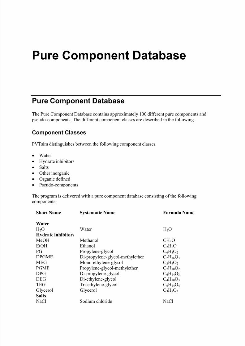
The Pure Component Database contains approximately 100 different pure components and
pseudo-components. The different component classes are described in the following.
Component Classes
PVTsim distinguishes between the following component classes
• Water• Hydrate inhibitors• Salts• Other inorganic
• Organic defined• Pseudo-components
The program is delivered with a pure component database consisting of the followingcomponents
Short Name Systematic Name Formula Name
Water
H2O Water H2OHydrate inhibitors
MeOH Methanol CH4OEtOH Ethanol C2H6OPG Propylene-glycol C6H8O2 DPGME Di-propylene-glycol-methylether C7H16O3 MEG Mono-ethylene-glycol C2H6O2 PGME Propylene-glycol-methylether C7H10O2 DPG Di-propylene-glycol C6H14O3 DEG Di-ethylene-glycol C4H10O3 TEG Tri-ethylene-glycol C6H14O4 Glycerol Glycerol C3H8O3
Salts NaCl Sodium chloride NaCl
7/18/2019 PVTsim Tutorial Calsep
http://slidepdf.com/reader/full/pvtsim-tutorial-calsep 8/140
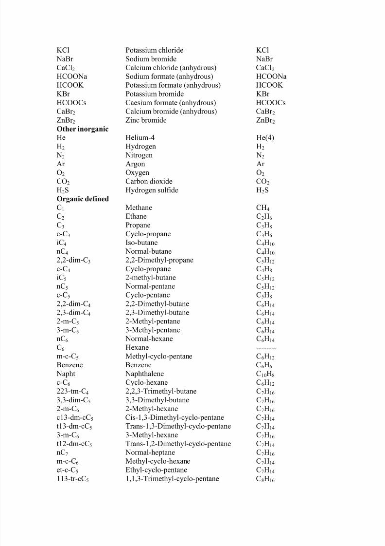
KCl Potassium chloride KCl NaBr Sodium bromide NaBrCaCl2 Calcium chloride (anhydrous) CaCl2 HCOONa Sodium formate (anhydrous) HCOONaHCOOK Potassium formate (anhydrous) HCOOK
KBr Potassium bromide KBrHCOOCs Caesium formate (anhydrous) HCOOCsCaBr 2 Calcium bromide (anhydrous) CaBr 2 ZnBr 2 Zinc bromide ZnBr 2 Other inorganic
He Helium-4 He(4)H2 Hydrogen H2
N2 Nitrogen N2 Ar Argon ArO2 Oxygen O2 CO2 Carbon dioxide CO2
H2S Hydrogen sulfide H2SOrganic defined
C1 Methane CH4 C2 Ethane C2H6 C3 Propane C3H8 c-C3 Cyclo-propane C3H6 iC4 Iso-butane C4H10 nC4 Normal-butane C4H10 2,2-dim-C3 2,2-Dimethyl-propane C5H12 c-C4 Cyclo-propane C4H8 iC5 2-methyl-butane C5H12 nC5 Normal-pentane C5H12 c-C5 Cyclo-pentane C5H8 2,2-dim-C4 2,2-Dimethyl-butane C6H14 2,3-dim-C4 2,3-Dimethyl-butane C6H14 2-m-C5 2-Methyl-pentane C6H14 3-m-C5 3-Methyl-pentane C6H14 nC6 Normal-hexane C6H14 C6 Hexane --------m-c-C5 Methyl-cyclo-pentane C6H12 Benzene Benzene C6H6
Napht Naphthalene C10H8 c-C6 Cyclo-hexane C6H12 223-tm-C4 2,2,3-Trimethyl-butane C7H16 3,3-dim-C5 3,3-Dimethyl-butane C7H16 2-m-C6 2-Methyl-hexane C7H16 c13-dm-cC5 Cis-1,3-Dimethyl-cyclo-pentane C7H14 t13-dm-cC5 Trans-1,3-Dimethyl-cyclo-pentane C7H14 3-m-C6 3-Methyl-hexane C7H16 t12-dm-cC5 Trans-1,2-Dimethyl-cyclo-pentane C7H14 nC7 Normal-heptane C7H16 m-c-C6 Methyl-cyclo-hexane C7H14
et-c-C5 Ethyl-cyclo-pentane C7H14 113-tr-cC5 1,1,3-Trimethyl-cyclo-pentane C8H16
7/18/2019 PVTsim Tutorial Calsep
http://slidepdf.com/reader/full/pvtsim-tutorial-calsep 9/140
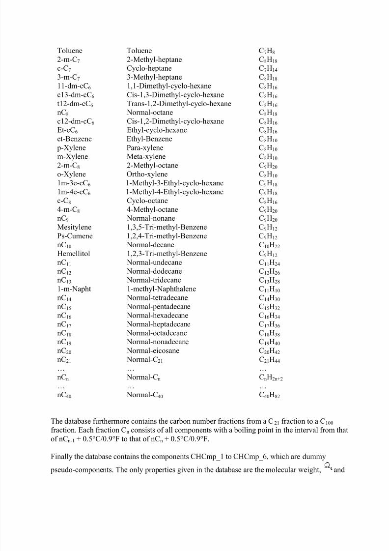
Toluene Toluene C7H8 2-m-C7 2-Methyl-heptane C8H18 c-C7 Cyclo-heptane C7H14 3-m-C7 3-Methyl-heptane C8H18 11-dm-cC6 1,1-Dimethyl-cyclo-hexane C8H16
c13-dm-cC6 Cis-1,3-Dimethyl-cyclo-hexane C8H16 t12-dm-cC6 Trans-1,2-Dimethyl-cyclo-hexane C8H16 nC8 Normal-octane C8H18 c12-dm-cC6 Cis-1,2-Dimethyl-cyclo-hexane C8H16 Et-cC6 Ethyl-cyclo-hexane C8H16 et-Benzene Ethyl-Benzene C8H10
p-Xylene Para-xylene C8H10 m-Xylene Meta-xylene C8H10 2-m-C8 2-Methyl-octane C9H20 o-Xylene Ortho-xylene C8H10 1m-3e-cC6 1-Methyl-3-Ethyl-cyclo-hexane C9H18
1m-4e-cC6 1-Methyl-4-Ethyl-cyclo-hexane C9H18 c-C8 Cyclo-octane C8H16 4-m-C8 4-Methyl-octane C9H20 nC9 Normal-nonane C9H20 Mesitylene 1,3,5-Tri-methyl-Benzene C9H12 Ps-Cumene 1,2,4-Tri-methyl-Benzene C9H12 nC10 Normal-decane C10H22 Hemellitol 1,2,3-Tri-methyl-Benzene C9H12 nC11 Normal-undecane C11H24 nC12 Normal-dodecane C12H26 nC13 Normal-tridecane C13H28 1-m-Napht 1-methyl-Naphthalene C11H10 nC14 Normal-tetradecane C14H30 nC15 Normal-pentadecane C15H32 nC16 Normal-hexadecane C16H34 nC17 Normal-heptadecane C17H36 nC18 Normal-octadecane C18H38 nC19 Normal-nonadecane C19H40 nC20 Normal-eicosane C20H42 nC21 Normal-C21 C21H44 … … …
nCn Normal-Cn CnH2n+2 … … …nC40 Normal-C40 C40H82
The database furthermore contains the carbon number fractions from a C21 fraction to a C100
fraction. Each fraction Cn consists of all components with a boiling point in the interval from thatof nCn-1 + 0.5°C/0.9°F to that of nCn + 0.5°C/0.9°F.
Finally the database contains the components CHCmp_1 to CHCmp_6, which are dummy
pseudo-components. The only properties given in the database are the molecular weight, and
7/18/2019 PVTsim Tutorial Calsep
http://slidepdf.com/reader/full/pvtsim-tutorial-calsep 10/140
, and the molecular weight will usually also have to be modified by the user. Othercomponent properties must be entered manually.
Component Properties
For each component the database holds the following component properties
• Name (short, systematic, and formula)• Molecular weight• Liquid density at atmospheric conditions (not needed for gaseous components)• Critical temperature (Tc)• Critical pressure (Pc)• Acentric factor ( )• Normal boiling point (T b)
• Weight average molecular weight (equal to molecular weight unless for pseudo-components)• Critical volume (Vc)• Vapor pressure model (classical or Mathias-Copeman)• Mathias-Copeman coefficients (only available for some components)• Temperature independent and temperature dependent term of the volume shift (or Peneloux)
parameter for either the SRK or PR equations
• Melting point depression ( )• Ideal gas absolute enthalpy at 273.15 K/0°C/32°F (Href )• Coefficients in ideal gas heat capacity (C p) polynomial• Melting point temperature (Tf )
• Enthalpy of melting ( )• PNA distribution (only for pseudo-components)• Wax fraction (only for n-paraffins and pseudo-components)• Asphaltene fraction (only for pseudo-components)• Parachor• Hydrate formation indicator (None, I, II, H and combinations)• Hydrate Langmuir constants• Number of ions in aqueous solution (only for salts)• Number of crystal water molecules per salt molecule (only for salts)• Pc of wax forming fractions (only for n-paraffins and pseudo-components)
• and in the SRK and PR equations
The component properties needed to calculate various physical properties and transport properties will usually be established as a part of the fluid characterization. It is however, also possible to input new components without entering all component properties and it is possible toinput compositions in characterized form.
Tc, Pc, , , , and molecular weight are required input for all components to perform
simulations. Whether the remaining component properties are needed or not depends on the
simulation to be performed.
7/18/2019 PVTsim Tutorial Calsep
http://slidepdf.com/reader/full/pvtsim-tutorial-calsep 11/140
The below table shows what component properties are needed to calculate a given property forgas and oil phases.
Physical or transport property Component properties needed
Volume Peneloux parameter *1)
Density Peneloux parameter *1)
Z factor Peneloux parameter *1)
Enthalpy (H) Ideal gas CP coefficients, Peneloux parameter *1) Entropy (S) Ideal gas CP coefficients, Peneloux parameter *1) Heat capacity (CP) Ideal gas CP coefficientsHeat capacity (CV) Ideal gas CP coefficients, Peneloux parameter *1) Kappa (CP/ CV) Ideal gas CP coefficients, Peneloux parameter *1) Joule-Thomson coefficient Ideal gas CP coefficients, Peneloux parameter *1) Velocity of sound Peneloux parameter *1) Viscosity Weight average molecular weight*2), Vc
*3)
Thermal conductivitySurface tension Parachor, Peneloux parameter *1)
*1) Only if an equation of state with Peneloux volume correction is used.*2) Only if corresponding states viscosity model selected.*3) Only if LBC viscosity model selected.
User Defined Components
User defined components may be added to the database. It is recommended to enter as manycomponent properties for these as possible. The following properties must be entered
• Component type• Name• Critical temperature (Tc)• Critical pressure (Pc)• Acentric factor ( )
• and
• Molecular weight (M)
For pseudo-components it is highly recommended also to enter the liquid density.
Missing Properties
PVTsim has a <Complete> option for estimating missing component properties for a fluidcomposition entered in characterized form. The number of missing properties estimated depends
on the properties entered manually. It is assumed that Tc, Pc, , , , and molecular weight
have all been entered. Below is shown what other properties are needed to estimate a givenmissing property and a reference is given to the section in the Method Documentation where the
property correlation is described.
Property Component properties Section where described
7/18/2019 PVTsim Tutorial Calsep
http://slidepdf.com/reader/full/pvtsim-tutorial-calsep 12/140
needed for estimation
Liquid density T independent term ofPeneloux parameter
SRK with Volume Correction.PR with Volume Correction.
Normal boiling point None Extrapolation of Plus Fraction.Weight average molecular
weight
Assumed equal to number
average molecular weight
-
Critical volume None Lohrenz-Bray-Clark (LBC) part of Viscosity section.
Vapor pressure model Not estimated -Mathias-Copeman coefficients Not estimated -T-independent term of SRKor PR Peneloux parameter
for defined components.Liquid density for pseudo-components
SRK with Volume Correctionor PR with Volume Correction
T-dependent term of SRK orPR Peneloux parameter
Not estimated for definedcomponents. Liquid densityfor pseudo-components
SRK with Volume Correctionor PR with Volume Correction
Melting point depression
( )
Only for pseudo-components.Viscosity data for anuninhibited/inhibited fluid.
Ideal gas absolute enthalpy at273.15 K/0°C/32°F (Href )
Molecular weight Compositional variation due togravity
Ideal gas Cp coefficients Not estimated for definedcomponents. Liquid densityfor pseudo-components
Enthalpy
Melting temperature (Tf ) Irrelevant for definedcomponents. None for pseudo-
components
Extended C7+ Characterization
Enthalpy of melting ( ) Irrelevant for definedcomponents. None for pseudo-components
Extended C7+ Characterization
PNA distribution Irrelevant for definedcomponents. Liquid densityfor pseudo-components
Estimation of PNADistribution
Wax fraction Irrelevant for definedcomponents. None for pseudo-components.
Extended C7+ Characterization
Asphaltene fraction Irrelevant for defined
components. Liquid densityfor pseudo-components
Asphaltenes
Parachor Not estimated for definedcomponents. Liquid densityfor pseudo-components
Gas/Oil interfacial tension.
Hydrate former or not Not estimated -Hydrate Langmuir constants Not estimated -
Number of ions in aqueoussolution (only for salts)
Not estimated -
Number of crystal water
molecules per salt molecule(only for salts)
Not estimated -

7/18/2019 PVTsim Tutorial Calsep
http://slidepdf.com/reader/full/pvtsim-tutorial-calsep 13/140
Pc of wax forming fraction Irrelevant for definedcomponents. None for pseudo-components
Extended C7+ Characterization
7/18/2019 PVTsim Tutorial Calsep
http://slidepdf.com/reader/full/pvtsim-tutorial-calsep 14/140
Composition Handling
Composition Handling
PVTsim distinguishes between the following fluid types
• Compositions with Plus fraction
• Compositions with No plus fraction
• Characterized compositions
Compositions with plus fraction are compositions as reported by PVT laboratories where the lastcomponent is a plus fraction residue. For this type of compositions the required input is mol%’sof all components and molecular weights and densities of all C7+ components (carbon numberfractions).
Compositions with No plus fraction require the same input as compositions with a plus fraction.In this case the heaviest component is not a residue but an actual component or a boiling pointcut and no extrapolation is performed. Gas mixtures with only a marginal content of C7+ components are usually classified as compositions with No plus fraction.
In the simulations characterized compositions are used. These are usually generated from a Plusfraction or No plus fraction type of composition. They may alternatively be entered manually.
Types of fluid analyses
When considering fluid composition input a distinction is made between the light components upto C6 which are always identified by gas chromatographic analysis, and the components heavierthan C6 which may be analyzed in different ways. Generally two types of fluid analyses are usedfor the C7+ components, both of which must deal with the fact that the number of isomericcomponents for the larger molecules makes a detailed analysis of all chemical speciesimpossible. These are true boiling point analyses (TBP) and a gas chromatographic (GC)analyses.
GC analysis
The GC analysis in various modifications is often used as it is relatively cheap, very fast, and because only a very small sample volume is required. Furthermore the GC analysis is much moredetailed than a TBP analysis. A GC analysis on the other hand suffers from the problem that
7/18/2019 PVTsim Tutorial Calsep
http://slidepdf.com/reader/full/pvtsim-tutorial-calsep 15/140
heavy ends may be lost in the analysis, especially heavy aromatics such as asphaltenes. The main problem with a GC analysis is however that no information is retained on molecular weight (M)and density of the cuts above C6. These are instead estimated from correlations. This in particularis a problem for the plus fraction residue properties, which are essential for a properrepresentation of the heaviest constituents of the fluid. To remedy this problem a GC
composition may be entered into PVTsim as follows.
Often a set of residue properties is available say for the C7+ fraction, while the measured GCcomposition often extends to e.g. C30. In this case one may enter the mol%'s to C30 together withthe M and density of the total C7+ fraction leaving the M and density fields blank for the higherC8 - C30 fractions. With this input, the program will be extrapolating from the C7+ fraction
properties, while honoring the reported composition for the fractions up to C30 under the mass balance constraints. If no information is available on the residue properties, one may as analternative lump back the composition to C7+ and estimate properties from there, which will often
provide equally accurate simulation results as with the detailed GC composition.
TBP Distillation
The TBP distillation requires a larger sample volume, typically 50 – 200 cc and is more timeconsuming. The method separates the components heavier than C6 into fractions bracketed by the
boiling points of the normal alkanes. For instance, the C7 fraction refers to all species, whichdistil off between the boiling point of nC6 + 0.5°C/0.9°F, and the boiling point of nC7 +0.5°C/0.9°F, regardless of how many carbon atoms these components contain. Each of thefractions distilled off is weighed and the molecular weights and densities are determinedexperimentally. The density and molecular weight in combination provide valuable informationto the characterization procedure on the PNA distribution. Aromatic components for instancehave a higher density and a lower Mw than paraffinic components. The residue from thedistillation is also analyzed for amount, M and density. These properties are important in thecharacterization procedure.
Whenever possible, it is recommended that input for PVTsim is generated based on a TBPanalysis. The accuracy of the characterization procedure relies on good values for densities andmolecular weights of the C7+ fractions. Parameters such as the Peneloux volume shift for theheavier pseudo-components are estimated based on the input densities, and consequently thequality of the input directly affects the density predictions of the equation of state (EOS) model.While the default values in PVTsim are generally considered to be reasonably accurate, they cannever be expected to match the characteristics on any given crude exactly, and thus experimental
values are much to be preferred.
Handling of pure components heavier than C6
When the compositional input is based on a GC analysis, there will often be defined components(pure chemical species) reported, which in the TBP-terminology would belong to a boiling pointfraction because it has a boiling point higher than nC6 + 0.5°C/0.9°F. Such components may beentered alongside with the boiling point fraction, which then represents the remaining unresolvedspecies within that boiling point interval. Before the entered composition is taken through thecharacterization procedure, the pure species are lumped into their respective boiling pointfraction and the properties of that fraction adjusted accordingly. After the characterization, the
pure species are split from the pseudo-component it ended up in, and the properties adjusted
7/18/2019 PVTsim Tutorial Calsep
http://slidepdf.com/reader/full/pvtsim-tutorial-calsep 16/140
accordingly. This procedure ensures that discrepancies between different component classes areavoided in the characterization.
Fluid handling operations
Quite often it becomes practical to mix two or more fluids and continue simulations with themixed composition. In PVTsim there are a number of facilities available for this purpose. Theseare ‘Mixing’, ‘Weaving’, ‘Recombination’ and ‘Characterization to the same Pseudo-components’.
Mixing
PVTsim may be used to mix or weave from 2 to 50 fluid compositions. A mixing will notnecessarily retain the pseudo-components of the individual compositions. Averaging the
properties of the pseudo-components in the individual compositions generates new pseudo-
components. Mixing may be performed on all types of compositions. For fluids characterized inPVTsim mixing is done on the level where the fluid has been characterized but not yet lumped.Each set of discrete fractions is mixed and the properties of the mixed fraction averaged on amass basis. Afterwards the mixed fluid is lumped to the specified number of components. If thetotal number of C7+ components in the fluids to be mixed exceeds the defaults number of pseudo-components (12), pseudo-components of approximately the same weight are lumped to get downto the desired number of pseudo-components in the mixed fluid.
Weaving
Weaving will maintain the pseudo-components of the individual compositions and can only be performed for characterized compositions. When weaving two fluids, all pseudo-componentsfrom all the original fluids are maintained in the resulting weaved fluid. This may lead to severalcomponents having the same name, and it is therefore advisable to tag the component names inorder to avoid confusion later on. The weaving option is useful to track specific components in a
process simulation or for allocation studies.
Recombination
Recombination is a mixing on volumetric basis performed for a given P and T (usually separatorconditions). Recombination can only be performed for two compositions, an oil and a gas
composition. The recombination option is often used to combine a separator gas phase and aseparator oil phase to get the feed to the separator. When the two fluids are recombined, the GORand liquid density at separator conditions must be input. Alternatively the saturation point of therecombined fluid can be entered along with the liquid density. When the GOR is specified, the
program determines the number of mols corresponding to the input volumes and simply mixesthe two fluids based on this. When the saturation pressure is specified, the recombination isiterative (i.e. how much of the gas should be added to yield this saturation pressure).
Characterization to the same pseudo-components
The goal of characterizing fluids to the same pseudo-components is to obtain a number of fluids,which are all represented by the same component set. Numerically this is done in a similar
7/18/2019 PVTsim Tutorial Calsep
http://slidepdf.com/reader/full/pvtsim-tutorial-calsep 17/140
fashion as the mixing operation with the only difference that the same pseudos logic keeps trackof the molar amount of each pseudo-component contained in each individual fluid.
The characterization to the same pseudo-components option is a very powerful tool, and can beapplied for a number of tasks. In compositional pipeline simulations where different streams are
mixed during the calculations or in compositional reservoir simulations where zones withdifferent PVT behavior are considered, mixing is straightforward when all fluids have the same
pseudo-components. It is furthermore possible to do regression in combination with thecharacterization to the same pseudos, in which case one may put special emphasis on fluids forwhich PVT data sets are available. In this case the data sets will also affect the characterization ofthe fluids for which no PVT data exist.
Characterization to same pseudo-components is described in more detail in the section ofCharacterization of Heavy Hydrocarbons.
7/18/2019 PVTsim Tutorial Calsep
http://slidepdf.com/reader/full/pvtsim-tutorial-calsep 18/140
Flash Algorithms
Flash Algorithms
The flash algorithms of PVTsim are the backbone of all equilibrium calculations performed in
the various simulation options. The terminology behind the different flash options are describedin the following.
PT Flash
The input to a PT flash calculation consists of
• Molar composition of feed (z)• Pressure (P) and temperature (T)
A flash results consists of
• Number of phases• Amounts and molar compositions of each phase• Compressibility factor (Z) or density of each phase
Flash Algorithms
PVTsim makes use of the following flash algorithms
• PT non aqueous (Gas and oil)
• PT aqueous (Gas, oil, and aqueous)
• PT multi phase (Gas, max. two oils, and aqueous)
• PH (Gas, oil, and aqueous)
• PS (Gas, oil, and aqueous)
• VT (Gas, oil, and aqueous)
7/18/2019 PVTsim Tutorial Calsep
http://slidepdf.com/reader/full/pvtsim-tutorial-calsep 19/140
• UV (Gas, oil, and aqueous)
• HS (Gas, oil, and aqueous)
Specific PT flash options considering the appropriate solid phases are used in the hydrate, wax,
and asphaltene options.
A flash calculation assumes thermodynamic equilibrium. The thermodynamic models availablein PVTsim are the Soave-Redlich-Kwong (SRK) equation of state, the Peng-Robinson (PR)equation of state, and the Peng-Robinson 78 (PR78) equation of state. These equations are
presented in Equation of State section. To apply an equation of state, a number of properties areneeded for each component contained in the actual mixture. These are established through a C7+-characterization as outlined in the section on Characterization of Heavy Hydrocarbons.
PVTsim uses the PT flash algorithms of Michelsen (1982a, 1982b). They are based on the principle of Gibbs energy minimization. In a flash process a mixture will settle in the state atwhich its Gibbs free energy
∑=
= N
1iiiµnG
is at a minimum. ni is the number of mols present of component i and is the chemical potentialof component i. The chemical potential can be regarded as the “escaping tendency” ofcomponent i, and the way to escape is to form an additional phase. Only one phase is formed ifthe total Gibbs energy increases for all possible trial compositions of an additional phase. Two ormore phases will form, if it is possible to separate the mixture into two phases having a totalGibbs energy, lower than that of the single phase. With two phases (I and II) present inthermodynamic equilibrium, each component will have equal chemical potentials in each phase
IIi
Ii µµ =
The final number of phases and the phase compositions are determined as those with the lowesttotal Gibbs energy.
The calculation of whether a given mixture at a specified (P,T) separates into two or more phasesis called a stability analysis. The starting point is the Gibbs energy, G0, of the mixture as a single
phase
G0 = G(n1, n2, n3,……,n N)
ni stands for the number of mols of type i present in the mixture, and N is the number of differentcomponents.
The situation is considered where the mixture separates into two phases (I and II) of the
compositions (n1 - , n2 - , n3 - …., n N - ) and ( , , ……, ) where is small. TheGibbs energy of phase I may be approximated by a Taylor series expansion truncated after the
first order term
7/18/2019 PVTsim Tutorial Calsep
http://slidepdf.com/reader/full/pvtsim-tutorial-calsep 20/140
∑=
∂∂
−= N
1i ni
ii01 n
GεGG
The Gibbs energy of the second phase is found to be
GII = G ( , , ,……, )
The change in Gibbs energy due to the phase split is hence
( ) ∑∑==
−=−=−+= N
1i0iIIii0iIIi
N
1ii0III ))(µ)((µyε))(µ(µεGGG∆G
where , and yi is the mol fraction of component i in phase II. The sub-indices 0 and IIrefer to the single phase and to phase II, respectively. Only one phase is formed if is greater
than zero for all possible trial compositions of phase II. The chemical potential, , may beexpressed in terms of the fugacity, f i, as follows
)P1nlnzRT(1nµf 1nRTµµ ii0ii
0ii +++=+= ϕ
where is a standard state chemical potential, a fugacity coefficient, z a mol fraction, P the pressure, and the sub-index i stands for component i. The standard state is in this case the pure
component i at the temperature and pressure of the system. The equation for may then berewritten to
∑=
−−+= N
1i0iiIIiii ))1n(zln)1n(y(1ny
εRT
∆Gϕ ϕ
where zi is the mol fraction of component i in the total mixture. The stability criterion can now beexpressed in terms of mol fractions and fugacity coefficients. Only one phase exists if
∑= >−−+
N
1i 0iiIIiii0))ln(zln)ln(y(lny
ϕ ϕ
for all trial compositions of phase II. A minimum in G will at the same time be a stationary point.A stationary point must satisfy the equation
k )ln(lnz)ln(yln 0iiIIii =−−+
where k is independent of component index. Introducing new variables, Yi, given by
ln Yi = ln yi – k
the following equation may be derived
7/18/2019 PVTsim Tutorial Calsep
http://slidepdf.com/reader/full/pvtsim-tutorial-calsep 21/140
1n Yi = 1n zi + 1n( )0 – 1n( )II
PVTsim uses the following initial estimate for the ratio K i between the mol fraction ofcomponent i in the vapor phase and in the liquid phase
−= )
TT(15.42exp
PPK cici
i
where
K i= yi/xi
and Tci is the critical temperature and Pci the critical pressure of component i. As initial estimatesfor Yi are used K izi, if phase 0 is a liquid and zi/K i, if phase 0 is a vapor. The fugacity
coefficients, ( )II, corresponding to the initial estimates for Yi are determined based on these
fugacity coefficients, new Yi-value are determined, and so on. For a single-phase mixture thisdirect substitution calculation will either converge to the trivial solution (i.e. to two identical phases) or to Yi-values fulfilling the criterion
∑=
≤ N
1ii 1Y
which corresponds to a non-negative value of the constant k. A negative value of k would be anindication of the presence of two or more phases. In the two-phase case the molar compositionobtained for phase II is a good starting point for the calculation of the phase compositions. Fortwo phases in equilibrium, three sets of equations must be satisfied. These are
Materiel balance equations
( ) ( N1,2,3,...,i,zxβ1βy iii )==−+
Equilibrium equations
( ) N1,2,3,...,i,xy Lii
Vii == ϕ ϕ
Summation of mol fractions
( ) N1,2,3,...,i,0)x(y N
1iii ==−∑
=
In these equations xi, yi and zi are mol fractions in the liquid phase, the vapor phase and the total
mixture, respectively. is the molar fraction of the vapor phase. and are the fugacitycoefficients of component i in the vapor and liquid phases calculated from the equation of state.There are (2N + 1) equations to solve with (2N + 3) variables, namely (x1, x2, x3,…, x N), (y1, y2,
y3,….,y N), , T and P. With T and P specified, the number of variables equals the number ofequations. The equations can be simplified by introducing the equilibrium ratio or K-factor, K i =
yi/xi. The following expressions may then be derived for xi and yi
7/18/2019 PVTsim Tutorial Calsep
http://slidepdf.com/reader/full/pvtsim-tutorial-calsep 22/140
( ) ( )
( ) N1,2,3,...,i,xK y
N1,2,3,...,i,1K β1
zx
iii
i
ii
==
=−+
=
and for K i
( ) N1,2,3,...,i,K Vi
Li
i ==ϕ
ϕ
The above (2N+1) equations may then be reduced to the following (N+1) equations
( ) N1,2,3,...,i,ln
lnK ln
Vi
Li
i ==ϕ
ϕ
∑ ∑=
=−+−=−i
N
1iiiiii 01))β(K 1)/(1(K z)x(y
For a given total composition, a given (T, P) and K i estimated from the stability analysis, an
estimate of may be derived. This will allow new estimates of xi and yi to be derived and the K-
factors to be recalculated. A new value of is calculated and so on. This direct substitutioncalculation may be repeated until convergence. For more details on the procedure it isrecommended to consult the articles of Michelsen (1982a, 1982b).
For a system consisting of J phases the mass balance equation is
0H
1)(K z N
1i i
imi =−∑
=
where
1)(K β1H1 j
1m
mi
mi −+= ∑
−
=
m
β is the molar fraction of phase m. equals the ratio of mol fractions of component i in phasem and phase J. The phase compositions may subsequently be found from
( )
( ) N1,2,3,...,i,H
zy
J1,2,3,...,m N;1,2,3,...,i,H
K zy
i
iJi
i
miim
i
==
===
where and are the mol fractions of component i in phase m and phase J, respectively.
7/18/2019 PVTsim Tutorial Calsep
http://slidepdf.com/reader/full/pvtsim-tutorial-calsep 23/140
Other Flash Specifications
P and T are not always the most convenient flash specifications to use. Some of the processestaking place during oil and gas production are not at a constant P and T. Passage of a valve mayfor example be approximated as a constant enthalpy (H) process and a compression as a constant
entropy (S) process. The temperature after a valve may therefore be simulated by initially performing a PT flash at the conditions at the inlet to the valve. If the enthalpy is assumed to bethe same at the outlet, the temperature at the outlet can be found from a PH flash with P equal tothe outlet pressure and H equal to the enthalpy at the inlet. A PT flash followed by a PS flashmay similarly be used to determine an approximate temperature after a compressor.
To perform a PH or a PS flash an estimate has to be provided for the temperature. PVTsimassumes a temperature of 300 K/26.85°C/80.33°F. Two object functions are defined. These arefor a two-phase PH flash
∑=−=
N
1iiii1 1)ζ(K zg
spec2 HHg −=
where
( )1K β1ς ii −+=
H is total molar enthalpy for the estimated phase compositions, and Hspec is the specified molarenthalpy. At convergence both g1 and g2 are zero. The iteration procedure is described in
Michelsen (1986).
Other flash specifications are VT, UV and HS. V is the molar volume and T the absolutetemperature. A VT specification is useful to for example determine the pressure in an offshore
pipeline during shutdown. U is the internal energy. A dynamic flow problem may sometimesmore conveniently be expressed in U and V than in P and T.
Phase Identification
If a PT flash calculation for an oil or gas mixture shows existence of two phases, the phase of thelower density will in general be assumed to be gas or vapor and the phase of the higher density
liquid or oil. In the case of a single-phase solution it is less obvious whether to consider thesingle phase to be a gas or a liquid. There exists no generally accepted definition to distinguish agas from a liquid. Since the terms gas and oil are very much used in the oil industry, a criterion isneeded for distinguishing between the two types of phases.
The following phase identification criteria are used in PVTsim
Liquid if
7/18/2019 PVTsim Tutorial Calsep
http://slidepdf.com/reader/full/pvtsim-tutorial-calsep 24/140
1. The pressure is lower than the critical pressure and the temperature lower than the bubble point temperature.
2. The pressure is above the critical pressure and the temperature lower than the criticaltemperature.
Gas if
1. The pressure is lower than the critical pressure and the temperature higher than the dew point temperature.
2. The pressure is above the critical pressure and the temperature higher than the criticaltemperature.
In the flash options handling water, a phase containing more than 80 mol% total of thecomponents water, hydrate inhibitors and salts is identified as an aqueous phase.
Components Handled by Flash Algorithms
The non-aqueous PT-flash algorithm handles the following component classes
• Other inorganic• Organic defined• Pseudo-components
The PT aqueous and multiflash algorithms handle
• Water• Hydrate inhibitors• Other inorganic• Organic defined• Pseudo-components• Salts
The PH, PS, VT, UV, and HS flash algorithms handle
• Water• Hydrate inhibitors• Other inorganic• Organic defined• Pseudo-components
References
Michelsen, M.L., “The Isothermal Flash Problem. Part I: Stability”, Fluid Phase Equilibria 9,1982a, 1.

7/18/2019 PVTsim Tutorial Calsep
http://slidepdf.com/reader/full/pvtsim-tutorial-calsep 25/140
Michelsen, M.L., “The Isothermal Flash Problem. Part II: Phase-Split Calculation”, Fluid PhaseEquilibria 9, 1982b, 21.
Michelsen, M.L., “Multiphase Isenthalpic and Isentropic Flash Algorithms”, SEP Report 8616,Institut for Kemiteknik, The Technical University of Denmark, 1986
7/18/2019 PVTsim Tutorial Calsep
http://slidepdf.com/reader/full/pvtsim-tutorial-calsep 26/140
Phase Envelope and SaturationPoint Calculation
Phase Envelope and Saturation Point Calculation
No aqueous components
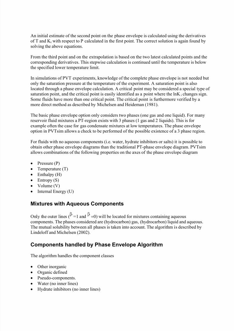
A phase envelope consists of corresponding values of T and P for which a phase fraction of agiven mixture equals a specified value. The phase fraction can either be a mol fraction or avolume fraction. The phase envelope option in PVTsim (Michelsen, 1980) may be used to
construct dew and bubble point lines, i.e. corresponding values of T and P for which equals 1
or 0, respectively. Also inner lines (0< <1) may be constructed.
The construction of the outer phase envelope ( =1 and =0) and inner molar lines follows the procedure outlined below. The first (T, P) value of a phase envelope is calculated by choosing afairly low pressure (P). The default in PVTsim is 5 Bar/4.93 atm/72.52 psi. An initial estimate ofthe equilibrium factors (K i = yi/xi) is obtained from the following equation
−= )
T
T5.42(1exp
P
PK cici
i
This equation and the mass balance equation
∑ ∑= =
=−+−=− N
1i
N
1iiiiii 01))β(K 1)/(1(K z)x(y
are solved for T and equal to the specified vapor mol fraction. The correct value of T issubsequently calculated by solving this equation in conjunction with
Vi
Li
iln
lnlnK
ϕ
ϕ =
where the liquid (L) and vapor (V) phase fugacity coefficients, , are found using the equationof state.
7/18/2019 PVTsim Tutorial Calsep
http://slidepdf.com/reader/full/pvtsim-tutorial-calsep 27/140
An initial estimate of the second point on the phase envelope is calculated using the derivativesof T and K i with respect to P calculated in the first point. The correct solution is again found bysolving the above equations.
From the third point and on the extrapolation is based on the two latest calculated points and thecorresponding derivatives. This stepwise calculation is continued until the temperature is belowthe specified lower temperature limit.
In simulations of PVT experiments, knowledge of the complete phase envelope is not needed butonly the saturation pressure at the temperature of the experiment. A saturation point is alsolocated through a phase envelope calculation. A critical point may be considered a special type ofsaturation point, and the critical point is easily identified as a point where the lnK i changes sign.Some fluids have more than one critical point. The critical point is furthermore verified by amore direct method as described by Michelsen and Heideman (1981).
The basic phase envelope option only considers two phases (one gas and one liquid). For manyreservoir fluid mixtures a PT-region exists with 3 phases (1 gas and 2 liquids). This is forexample often the case for gas condensate mixtures at low temperatures. The phase envelopeoption in PVTsim allows a check to be performed of the possible existence of a 3 phase region.
For fluids with no aqueous components (i.e. water, hydrate inhibitors or salts) it is possible toobtain other phase envelope diagrams than the traditional PT-phase envelope diagram. PVTsimallows combinations of the following properties on the axes of the phase envelope diagram
• Pressure (P)
• Temperature (T)• Enthalpy (H)• Entropy (S)• Volume (V)• Internal Energy (U)
Mixtures with Aqueous Components
Only the outer lines ( =1 and =0) will be located for mixtures containing aqueouscomponents. The phases considered are (hydrocarbon) gas, (hydrocarbon) liquid and aqueous.
The mutual solubility between all phases is taken into account. The algorithm is described byLindeloff and Michelsen (2002).
Components handled by Phase Envelope Algorithm
The algorithm handles the component classes
• Other inorganic• Organic defined• Pseudo-components.
• Water (no inner lines)• Hydrate inhibitors (no inner lines)
7/18/2019 PVTsim Tutorial Calsep
http://slidepdf.com/reader/full/pvtsim-tutorial-calsep 28/140
The saturation point algorithm used in the saturation point option and the PVT simulations is also
based on the phase envelope algorithm, but does not handle water and hydrate inhibitors.
References
Lindeloff, N. and Michelsen, M.L., “Phase Envelope Calculations for Hydrocarbon-WaterMixtures”, SPE 77385, SPE ATCE in San Antonio, Tx, September 29 – October 2, 2002.
Michelsen, M.L., “Calculation of Phase Envelopes and Critical Points for MulticomponentMixtures”, Fluid Phase Equilibria, 1980, 4, pp. 1-10.
Michelsen, M.L. and Heidemann, R.A., “Calculation of Critical Points from Cubic Two-ConstantEquations of State”, AIChE J., 27, 1981, pp. 521-523.
7/18/2019 PVTsim Tutorial Calsep
http://slidepdf.com/reader/full/pvtsim-tutorial-calsep 29/140
Equations of State
Equations of State
The phase equilibrium calculations in PVTsim are based on one of the following equations
• Soave-Redlich-Kwong (SRK) (Soave, 1972)• Peng-Robinson (PR) (Peng and Robinson, 1976)• Modified Peng-Robinson (PR78) (Peng and Robinson, 1978)
All equations may be used with or without Peneloux volume correction (Peneloux et al., 1982). Aconstant or a temperature dependent Peneloux correction may be used. The temperaturedependent volume correction is determined to comply with the ASTM 1250-80 correlation forvolume correction factors for stable oils (Pedersen et al., 2002).
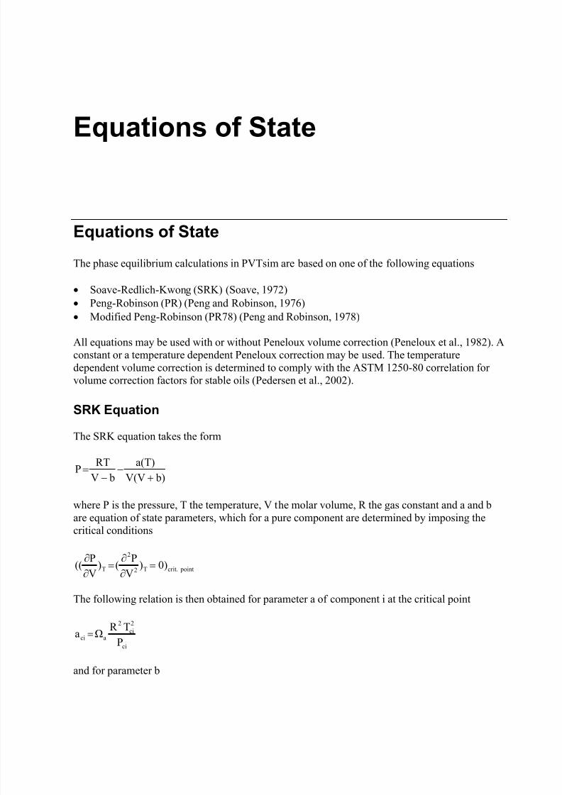
SRK Equation
The SRK equation takes the form
b)V(V
a(T)
bV
RTP
+−
−=
where P is the pressure, T the temperature, V the molar volume, R the gas constant and a and bare equation of state parameters, which for a pure component are determined by imposing thecritical conditions
pointcrit.T2
2
T 0))V
P()
V
P(( =
∂∂
=∂∂
The following relation is then obtained for parameter a of component i at the critical point
ci
2ci
2
aciP
TR Ωa =
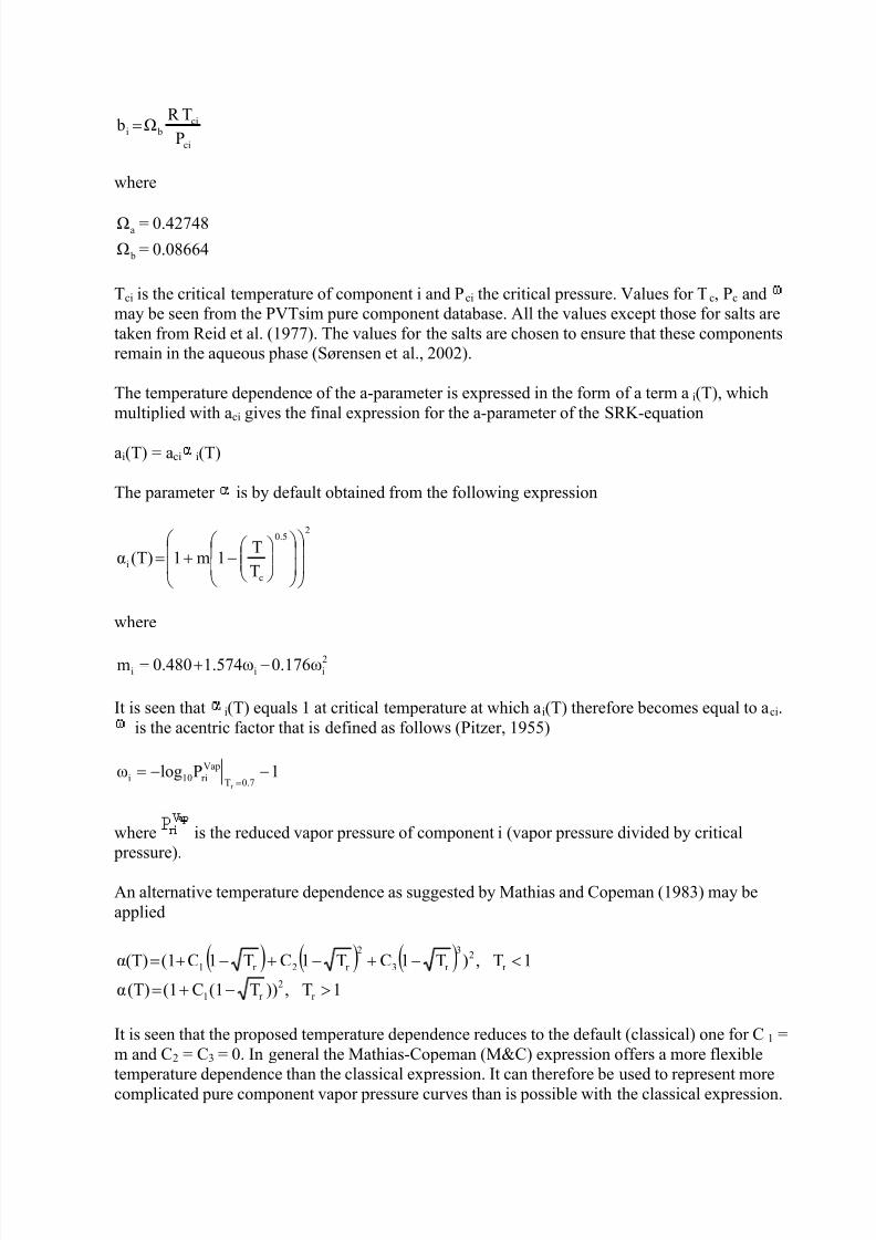
and for parameter b
7/18/2019 PVTsim Tutorial Calsep
http://slidepdf.com/reader/full/pvtsim-tutorial-calsep 30/140
ci
ci bi P
TR Ω b =
where
aΩ = 0.42748
bΩ = 0.08664
Tci is the critical temperature of component i and Pci the critical pressure. Values for Tc, Pc andmay be seen from the PVTsim pure component database. All the values except those for salts aretaken from Reid et al. (1977). The values for the salts are chosen to ensure that these componentsremain in the aqueous phase (Sørensen et al., 2002).
The temperature dependence of the a-parameter is expressed in the form of a term ai(T), whichmultiplied with aci gives the final expression for the a-parameter of the SRK-equation
ai(T) = aci i(T)
The parameter is by default obtained from the following expression
20.5
c
iT
T1m1(T)α
−+=
where
2iii 0.176ω1.574ω0.480m −+=
It is seen that i(T) equals 1 at critical temperature at which ai(T) therefore becomes equal to aci.is the acentric factor that is defined as follows (Pitzer, 1955)
1Plogω0.7T
Vapri10i
r
−−==
where is the reduced vapor pressure of component i (vapor pressure divided by critical
pressure).
An alternative temperature dependence as suggested by Mathias and Copeman (1983) may beapplied
( ) ( ) ( ) 1T,)T1CT1CT1C(1α(T) r 23
r 3
2
r 2r 1 <−+−+−+=
1T,))T(1C(1(T)α r 2
r 1 >−+=
It is seen that the proposed temperature dependence reduces to the default (classical) one for C1 =m and C2 = C3 = 0. In general the Mathias-Copeman (M&C) expression offers a more flexible
temperature dependence than the classical expression. It can therefore be used to represent morecomplicated pure component vapor pressure curves than is possible with the classical expression.

7/18/2019 PVTsim Tutorial Calsep
http://slidepdf.com/reader/full/pvtsim-tutorial-calsep 31/140
M&C is not used default in PVTsim, but is it possible for the user to change temperaturedependence from classical to M&C and to enter M&C coefficients (C1, C2 and C3) when theseare not given in the PVTsim database. The M&C coefficients used in PVTsim are from Dahl(1991).
SRK with Volume Correction
With Peneloux volume correction the SRK equation takes the form
( )( )2c bVcV
a
bV
RTP
+++−
−=
The SRK molar volume, , and the Peneloux molar volume, V, are related as follows
cVV~
−=
The b parameter in the Peneloux equation is similarly related to the SRK b-parameter asfollows
c b~
b −=
The parameter c can be regarded as a volume translation parameter, and it is given by thefollowing equation
c = c’ + c’’ (T – 288.15)
where T is the temperature in K. The parameter c’ is the temperature independent volumecorrection and c’’ the temperature dependent volume correction. Per default the temperaturedependent volume correction c’’ is set to zero unless for C+ pseudo-components. In general thetemperature independent Peneloux volume correction for defined organics and “other organics”is found from the following expression
( )RAc
c Z0.29441P
RT0.40768c' −=
ZRA is the Racket compressibility factor
ZRA = 0.29056 – 0.08775
For some components, e.g. H2O, MEG, DEG, TEG, and CO2, the values have been found from pure component density data. For heavy oil fractions c is determined in two steps. The liquiddensity is known at 15°C/59°F from the composition input. By converting this density ( ) to amolar volume V = M/ , the c’ parameter can be found as the difference between this molarvolume and the SRK molar volume for the same temperature. Similarly c’’ is found as the
difference between the molar volume at 80°C/176°F given by the ASTM 1250-80 density
7/18/2019 PVTsim Tutorial Calsep
http://slidepdf.com/reader/full/pvtsim-tutorial-calsep 32/140
correlation and the Peneloux molar volume for the same temperature, where the Penelouxvolume is found assuming c=c’.
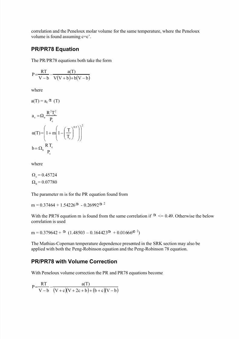
PR/PR78 Equation
The PR/PR78 equations both take the form
( ) ( ) bV b bVV
a(T)
bV
RTP
−++−
−=
where
a(T) = ac (T)
c
2c
2
ac P
TR Ωa =
20.5
cT
T1m1α(T)
−+=
c
c b P
TR b Ω=
where
aΩ = 0.45724 bΩ = 0.07780
The parameter m is for the PR equation found from
m = 0.37464 + 1.54226 - 0.26992 2
With the PR78 equation m is found from the same correlation if <= 0.49. Otherwise the belowcorrelation is used
m = 0.379642 + (1.48503 − 0.164423 + 0.016662
)
The Mathias-Copeman temperature dependence presented in the SRK section may also beapplied with both the Peng-Robinson equation and the Peng-Robinson 78 equation.
PR/PR78 with Volume Correction
With Peneloux volume correction the PR and PR78 equations become
( )( ) ( )( ) bVc b b2cVcV
a(T)
bV
RTP
−+++++
−
−
=
7/18/2019 PVTsim Tutorial Calsep
http://slidepdf.com/reader/full/pvtsim-tutorial-calsep 33/140
where c is a temperature dependent constant as presented in the SRK section. In general thetemperature independent Peneloux volume correction for defined organics and “other organics”is found from
)Z(0.25969P
RT
0.50033c' RAc
c −=
where ZRA is defined as for the Peneloux modification of the SRK equation. For othercomponents c’ is found as explained in the SRK section, which also explains how to determinethe temperature dependent term c”.
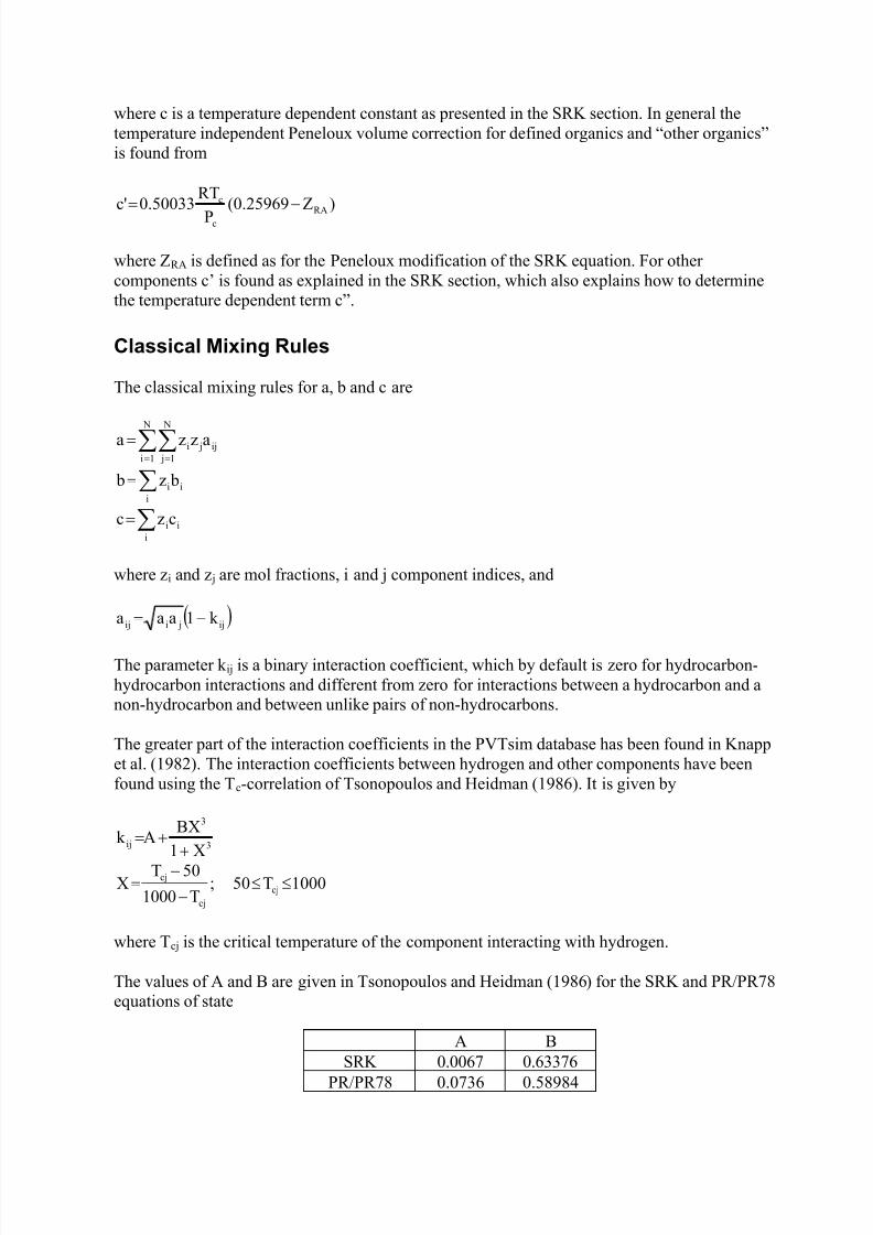
Classical Mixing Rules
The classical mixing rules for a, b and c are
∑∑= =
= N
1i
N
1 jij ji azza
∑=i
ii bz b
∑=i
iiczc
where zi and z j are mol fractions, i and j component indices, and
( )ij jiij k 1aaa −=
The parameter k ij is a binary interaction coefficient, which by default is zero for hydrocarbon-hydrocarbon interactions and different from zero for interactions between a hydrocarbon and anon-hydrocarbon and between unlike pairs of non-hydrocarbons.
The greater part of the interaction coefficients in the PVTsim database has been found in Knappet al. (1982). The interaction coefficients between hydrogen and other components have beenfound using the Tc-correlation of Tsonopoulos and Heidman (1986). It is given by
3
3
ij
X1
BXAk
+
+=
1000T50;T1000
50TX cj
cj
cj ≤≤−
−=
where Tcj is the critical temperature of the component interacting with hydrogen.
The values of A and B are given in Tsonopoulos and Heidman (1986) for the SRK and PR/PR78equations of state
A B
SRK 0.0067 0.63376PR/PR78 0.0736 0.58984
7/18/2019 PVTsim Tutorial Calsep
http://slidepdf.com/reader/full/pvtsim-tutorial-calsep 34/140
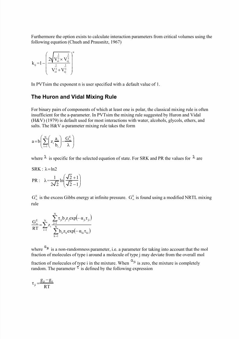
Furthermore the option exists to calculate interaction parameters from critical volumes using thefollowing equation (Chueh and Prausnitz, 1967)
n
3
1
cj3
1
ci
3
1
cj3
1
ci
ij
VV
VV21k
+
×−=
In PVTsim the exponent n is user specified with a default value of 1.
The Huron and Vidal Mixing Rule
For binary pairs of components of which at least one is polar, the classical mixing rule is often
insufficient for the a-parameter. In PVTsim the mixing rule suggested by Huron and Vidal(H&V) (1979) is default used for most interactions with water, alcohols, glycols, ethers, andsalts. The H&V a-parameter mixing rule takes the form
−
= ∑
=
∞ N
1i
E
i
ii
λ
G
b
az ba
where is specific for the selected equation of state. For SRK and PR the values for are
−+=
=
12
12ln
22
1λ :PR
ln2λ :SRK
EG∞ is the excess Gibbs energy at infinite pressure. is found using a modified NRTL mixing
rule
EG∞
( )
( )
∑
∑
∑
=
=
=∞
−
−
= N
li N
1k kikik k
N
1 j ji ji j j ji
i
E
ταexpz b
ταexpz bτ
zRT
G
where is a non-randomness parameter, i.e. a parameter for taking into account that the molfraction of molecules of type i around a molecule of type j may deviate from the overall mol
fraction of molecules of type i in the mixture. When is zero, the mixture is completelyrandom. The parameter is defined by the following expression
RT
ggτ
ii ji ji
−=
7/18/2019 PVTsim Tutorial Calsep
http://slidepdf.com/reader/full/pvtsim-tutorial-calsep 35/140
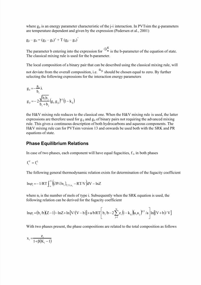
where g ji is an energy parameter characteristic of the j-i interaction. In PVTsim the g-parametersare temperature dependent and given by the expression (Pedersen et al., 2001)
g ji – gii = (g ji – gii)’ + T (g ji – gii)”
The parameter b entering into the expression for is the b-parameter of the equation of state.The classical mixing rule is used for the b-parameter.
The local composition of a binary pair that can be described using the classical mixing rule, will
not deviate from the overall composition, i.e. should be chosen equal to zero. By furtherselecting the following expressions for the interaction energy parameters
λ b
ag
i
iii −=
( ) ( ij
0.5
jjii ji
ji
ji k 1gg b b b b2g −
+−= )
the H&V mixing rule reduces to the classical one. When the H&V mixing rule is used, the latterexpressions are therefore used for gij and gii of binary pairs not requiring the advanced mixingrule. This gives a continuous description of both hydrocarbons and aqueous components. TheH&V mixing rule can for PVTsim version 13 and onwards be used both with the SRK and PRequations of state.
Phase Equilibrium Relations
In case of two phases, each component will have equal fugacities, f i, in both phases
Li
Vi f f =
The following general thermodynamic relation exists for determination of the fugacity coefficient
( )( )∫∞−−∂∂−=
V
nV,T,ii lnZdVRT/VnP/1/RTln j
ϕ
where ni is the number of mols of type i. Subsequently when the SRK equation is used, thefollowing relation can be derived for the fugacity coefficient
( )( ) ( )[ ] ( )( ) ( )[ ]V/ bVln/aaak 1z2/b bRTa/b bVV/lnlnZ1Z/b bln N
1 j
0.5 jiijiiii +
−−+−+−−= ∑
=
ϕ
With two phases present, the phase compositions are related to the total composition as follows
( )1K β1
zx
i
ii −+=
7/18/2019 PVTsim Tutorial Calsep
http://slidepdf.com/reader/full/pvtsim-tutorial-calsep 36/140
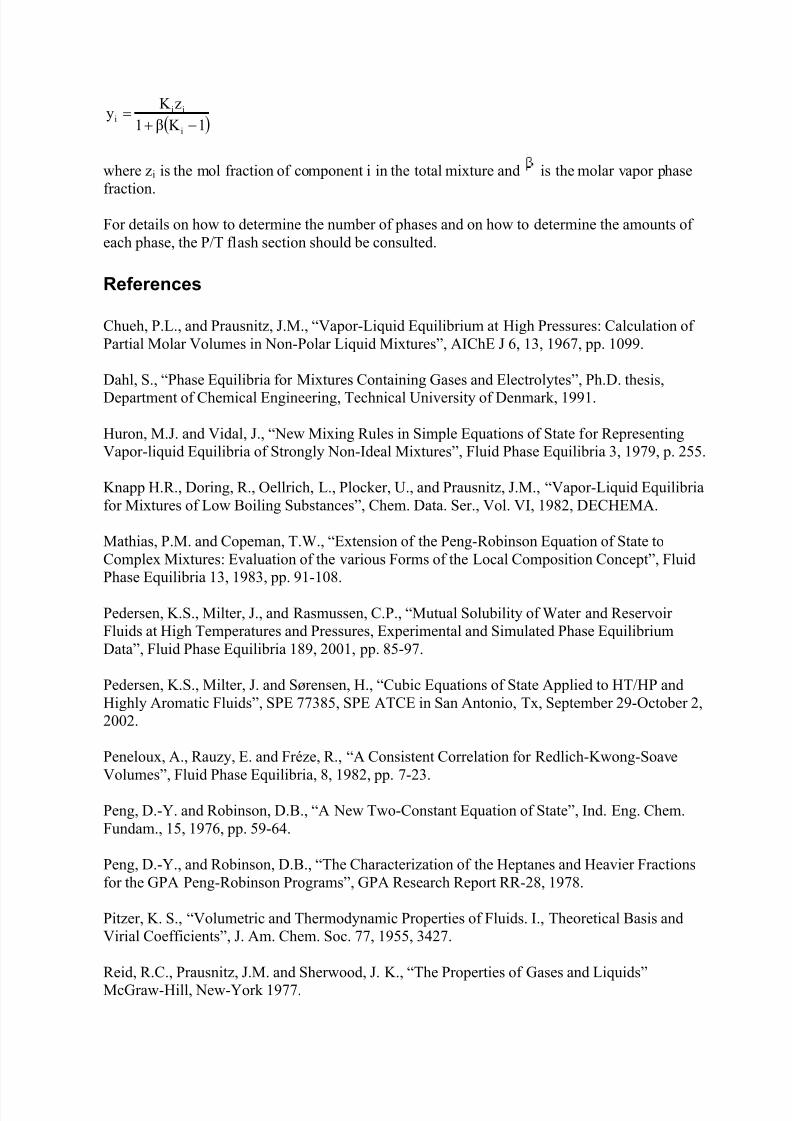
( )1K β1
zK y
i
iii −+
=
where zi is the mol fraction of component i in the total mixture and is the molar vapor phase
fraction.
For details on how to determine the number of phases and on how to determine the amounts ofeach phase, the P/T flash section should be consulted.
References
Chueh, P.L., and Prausnitz, J.M., “Vapor-Liquid Equilibrium at High Pressures: Calculation ofPartial Molar Volumes in Non-Polar Liquid Mixtures”, AIChE J 6, 13, 1967, pp. 1099.
Dahl, S., “Phase Equilibria for Mixtures Containing Gases and Electrolytes”, Ph.D. thesis,Department of Chemical Engineering, Technical University of Denmark, 1991.
Huron, M.J. and Vidal, J., “New Mixing Rules in Simple Equations of State for RepresentingVapor-liquid Equilibria of Strongly Non-Ideal Mixtures”, Fluid Phase Equilibria 3, 1979, p. 255.
Knapp H.R., Doring, R., Oellrich, L., Plocker, U., and Prausnitz, J.M., “Vapor-Liquid Equilibriafor Mixtures of Low Boiling Substances”, Chem. Data. Ser., Vol. VI, 1982, DECHEMA.
Mathias, P.M. and Copeman, T.W., “Extension of the Peng-Robinson Equation of State toComplex Mixtures: Evaluation of the various Forms of the Local Composition Concept”, Fluid
Phase Equilibria 13, 1983, pp. 91-108.
Pedersen, K.S., Milter, J., and Rasmussen, C.P., “Mutual Solubility of Water and ReservoirFluids at High Temperatures and Pressures, Experimental and Simulated Phase EquilibriumData”, Fluid Phase Equilibria 189, 2001, pp. 85-97.
Pedersen, K.S., Milter, J. and Sørensen, H., “Cubic Equations of State Applied to HT/HP andHighly Aromatic Fluids”, SPE 77385, SPE ATCE in San Antonio, Tx, September 29-October 2,2002.
Peneloux, A., Rauzy, E. and Fréze, R., “A Consistent Correlation for Redlich-Kwong-Soave
Volumes”, Fluid Phase Equilibria, 8, 1982, pp. 7-23.
Peng, D.-Y. and Robinson, D.B., “A New Two-Constant Equation of State”, Ind. Eng. Chem.Fundam., 15, 1976, pp. 59-64.
Peng, D.-Y., and Robinson, D.B., “The Characterization of the Heptanes and Heavier Fractionsfor the GPA Peng-Robinson Programs”, GPA Research Report RR-28, 1978.
Pitzer, K. S., “Volumetric and Thermodynamic Properties of Fluids. I., Theoretical Basis andVirial Coefficients”, J. Am. Chem. Soc. 77, 1955, 3427.
Reid, R.C., Prausnitz, J.M. and Sherwood, J. K., “The Properties of Gases and Liquids”McGraw-Hill, New-York 1977.
7/18/2019 PVTsim Tutorial Calsep
http://slidepdf.com/reader/full/pvtsim-tutorial-calsep 37/140
Soave, G., “Equilibrium Constants From a Modified Redlich-Kwong Equation of State”, Chem.Eng. Sci. 27, 1972, 1197.
Sørensen, H., Pedersen, K.S. and Christensen, P.L., "Modeling of Gas Solubility in
Brine", Organic Geochemistry 33, 2002, pp. 35-642.
Tsonopoulos, C., and Heidman, J.L., “High-Pressure Vapor-Liquid Equilibria with CubicEquations of State”, Fluid Phase Equilibria 29, 1986, pp. 391-414.
7/18/2019 PVTsim Tutorial Calsep
http://slidepdf.com/reader/full/pvtsim-tutorial-calsep 38/140
Characterization of HeavyHydrocarbons
Characterization of Heavy Hydrocarbons
To use a cubic equation of state as for example the SRK or the PR equations on oil and gascondensate mixtures the critical temperature, Tc, the critical pressure, Pc, and the acentric factor,
, must be known for each component of the mixture. Naturally occurring oil or gas condensatemixtures may contain thousands of different components. This number of components exceedswhat is practical in a usual phase equilibrium calculation. Some of the components must begrouped together and represented as pseudo-components. C7+-characterization consists inrepresenting the hydrocarbons with seven and more carbon atoms as a reasonable number of
pseudo-components and to find the needed equation of state parameters, Tc, Pc and , for these pseudo-components.
Classes of Components
Naturally occurring oil and gas condensate mixtures consist of three classes of components
Defined Components
These are per default N2, CO2, H2S, C1, C2, C3, iC4, nC4, iC5 and C6 in PVTsim. C6 is in PVTsimconsidered to be pure nC6.
C7+ Fractions
Each C7+ fraction contains hydrocarbons with boiling points within a given temperature interval.Carbon number fraction n consists of the components with a boiling point between that of nCn-1 +0.5°C/0.9°F and nCn + 0.5°C/0.9°F. The C7 fraction for example consists of the components witha boiling point between those of nC6 + 0.5°C/0.9°F and nC7 + 0.5°C/0.9°F . For the C7+-fractionsthe density at standard conditions (1 atm/14.969 psi and 15°C/59°F) and the molecular weightmust be input.
The Plus Fraction
The plus fraction consists of the components, which are too heavy to be separated in individualC7+-fractions. The average molecular weight and the density must be known.
7/18/2019 PVTsim Tutorial Calsep
http://slidepdf.com/reader/full/pvtsim-tutorial-calsep 39/140
Properties of C7+-Fractions
PVTsim supports two different characterization procedures
- Standard oil characterization to C80
- Heavy oil characterization to C200
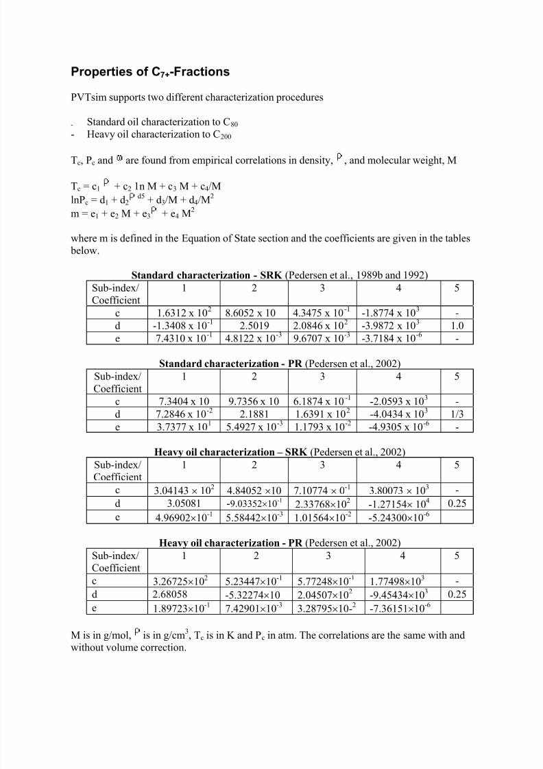
Tc, Pc and are found from empirical correlations in density, , and molecular weight, M
Tc = c1 + c2 1n M + c3 M + c4/MlnPc = d1 + d2
d5 + d3/M + d4/M2
m = e1 + e2 M + e3 + e4 M2
where m is defined in the Equation of State section and the coefficients are given in the tables below.
Standard characterization - SRK (Pedersen et al., 1989b and 1992) Sub-index/Coefficient
1 2 3 4 5
c 1.6312 x 10² 8.6052 x 10 4.3475 x 10⁻¹ -1.8774 x 10³ -d -1.3408 x 10⁻¹ 2.5019 2.0846 x 10² -3.9872 x 10³ 1.0e 7.4310 x 10⁻¹ 4.8122 x 10⁻³ 9.6707 x 10⁻³ -3.7184 x 10⁻⁶ -
Standard characterization - PR (Pedersen et al., 2002)Sub-index/Coefficient
1 2 3 4 5
c 7.3404 x 10 9.7356 x 10 6.1874 x 10⁻¹ -2.0593 x 10³ -d 7.2846 x 10⁻² 2.1881 1.6391 x 10² -4.0434 x 10³ 1/3e 3.7377 x 101 5.4927 x 10⁻³ 1.1793 x 10⁻² -4.9305 x 10⁻⁶ -
Heavy oil characterization – SRK (Pedersen et al., 2002)Sub-index/Coefficient
1 2 3 4 5
c 3.04143 × 10² 4.84052 ×10 7.10774 × 0-1 3.80073 × 10³ -d 3.05081 -9.03352×10⁻¹
2.33768×10² -1.27154× 10⁴ 0.25e 4.96902×10⁻¹ 5.58442×10⁻³ 1.01564×10⁻² -5.24300×10⁻⁶
Heavy oil characterization - PR (Pedersen et al., 2002)Sub-index/Coefficient
1 2 3 4 5
c 3.26725×10² 5.23447×10⁻¹ 5.77248×10⁻¹ 1.77498×10³ -d 2.68058
-5.32274×10 2.04507×10² -9.45434×10³ 0.25e 1.89723×10⁻¹ 7.42901×10⁻³ 3.28795×10⁻² -7.36151×10⁻⁶
M is in g/mol, is in g/cm3, Tc is in K and Pc in atm. The correlations are the same with andwithout volume correction.
7/18/2019 PVTsim Tutorial Calsep
http://slidepdf.com/reader/full/pvtsim-tutorial-calsep 40/140
Extrapolation of the Plus Fraction
Characterization of the plus fraction consists in
• Estimation of the molar distribution, i.e. mol fraction versus carbon number.
• Estimation of the density distribution, i.e. the density versus carbon number.• Estimation of the boiling point distribution, i.e. boiling point versus carbon number• Estimation of the molecular weight distribution, i.e. molecular weight versus carbon number.• Calculation of Tc, Pc and of the resulting pseudo-components.
The molar composition of the TBP-residue is estimated by assuming a logarithmic relationship between the molar concentration z N, of a given fraction and the corresponding carbon number,C N, for C N >7
C N = A1 + B1 lnz N
A1 and B1 are determined from the measured mol fraction and the measured molecular weight ofthe plus fraction.
The densities of the carbon number fractions contained in the plus fraction are estimated byassuming a logarithmic dependence of against carbon number.
The boiling points recommended by Katz and Firoozabadi (1978) are used up to C45. Thefollowing relation is used for heavier components
TB = 97.58 M0.3323 0.04609
where TB is in K and in g/cm3.
Estimation of PNA Distribution
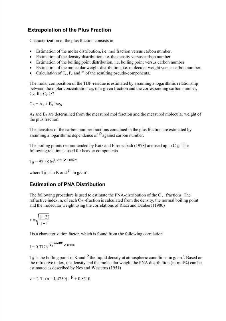
The following procedure is used to estimate the PNA-distribution of the C7+ fractions. Therefractive index, n, of each C7+-fraction is calculated from the density, the normal boiling pointand the molecular weight using the correlations of Riazi and Daubert (1980)
I1
2I1
n −
+
=
I is a characterization factor, which is found from the following correlation
I = 0.3773 0.9182
TB is the boiling point in K and the liquid density at atmospheric conditions in g/cm3. Based onthe refractive index, the density and the molecular weight the PNA distribution (in mol%) can beestimated as described by Nes and Westerns (1951)
v = 2.51 (n – 1.4750) - + 0.8510
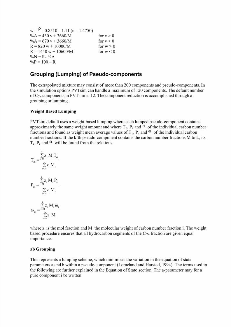
7/18/2019 PVTsim Tutorial Calsep
http://slidepdf.com/reader/full/pvtsim-tutorial-calsep 41/140
w = - 0.8510 – 1.11 (n – 1.4750)%A = 430 v + 3660/M for v > 0%A = 670 v + 3660/M for v < 0R = 820 w + 10000/M for w > 0R = 1440 w + 10600/M for w < 0
%N = R- %A%P = 100 – R
Grouping (Lumping) of Pseudo-components
The extrapolated mixture may consist of more than 200 components and pseudo-components. Inthe simulation options PVTsim can handle a maximum of 120 components. The default numberof C7+ components in PVTsim is 12. The component reduction is accomplished through agrouping or lumping.
Weight Based Lumping
PVTsim default uses a weight based lumping where each lumped pseudo-component containsapproximately the same weight amount and where Tc, Pc and of the individual carbon numberfractions and found as weight mean average values of Tc, Pc and of the individual carbonnumber fractions. If the k’th pseudo-component contains the carbon number fractions M to L, itsTc, Pc and will be found from the relations
∑
∑=
=
=L
Mi
ii
L
Miciii
ck
Mz
TMzT
∑
∑=
=
=L
Miii
L
Miciii
ck
Mz
PMzP
∑
∑=
=
=L
Miii
L
Miiii
ck
Mz
ωMzω
where zi is the mol fraction and Mi the molecular weight of carbon number fraction i. The weight based procedure ensures that all hydrocarbon segments of the C7+ fraction are given equalimportance.
ab Grouping
This represents a lumping scheme, which minimizes the variation in the equation of state parameters a and b within a pseudo-component (Lomeland and Harstad, 1994). The terms used inthe following are further explained in the Equation of State section. The a-parameter may for a
pure component i be written
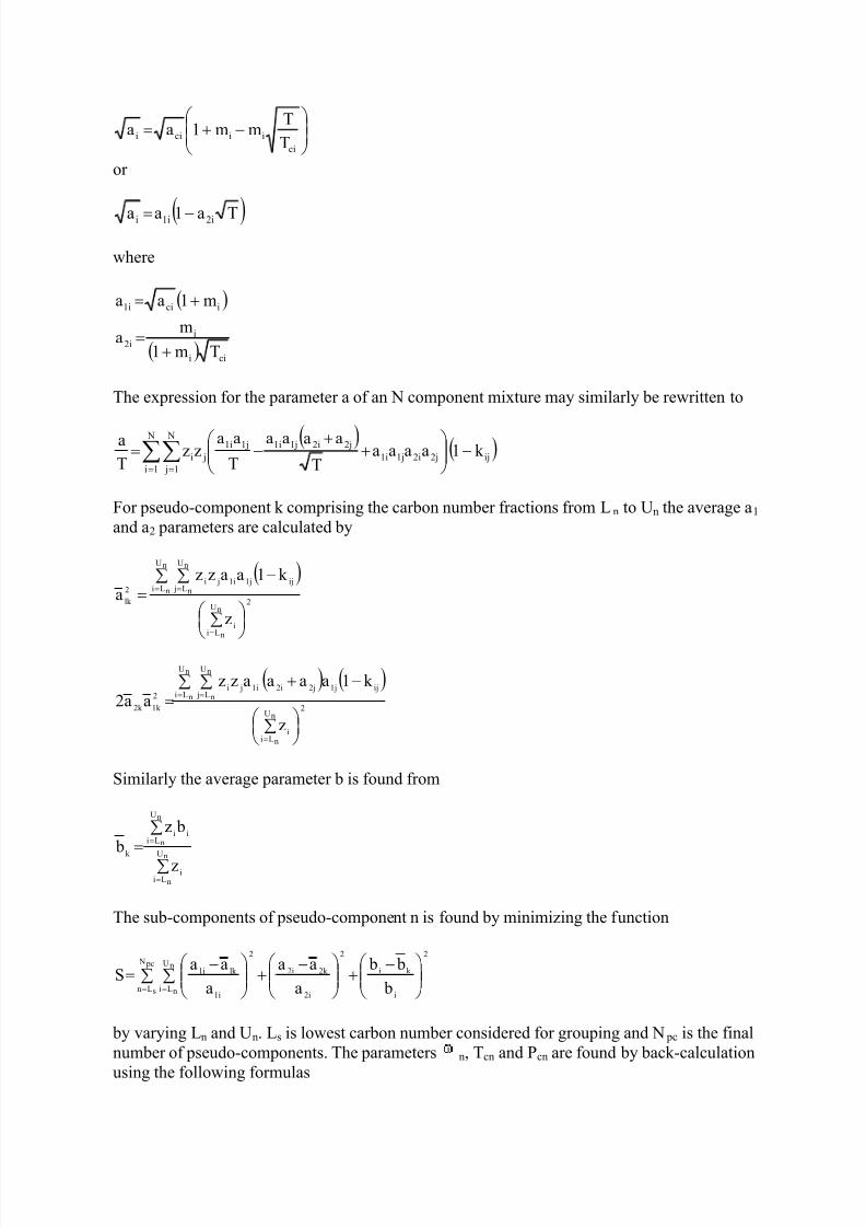
7/18/2019 PVTsim Tutorial Calsep
http://slidepdf.com/reader/full/pvtsim-tutorial-calsep 42/140
−+=
ci
iiciiT
Tmm1aa
or
( )Ta1aa 2i1ii −=
where
( )ici1i m1aa +=
( ) cii
i2i
Tm1
ma
+=
The expression for the parameter a of an N component mixture may similarly be rewritten to
( )( )∑∑
= =
−
+
+−=
N
1i
N
1 jij2j2i1j1i
2j2i1j1i1j1i ji k 1aaaa
T
aaaa
T
aazz
T
a
For pseudo-component k comprising the carbon number fractions from Ln to Un the average a1 and a2 parameters are calculated by
( )2
nU
nLi
i
nU
nLi
nU
nL jij1j1i ji
2
lk
z
k 1aazza
∑
∑ ∑ −=
=
= =
( ) ( )2
nU
nLii
nU
nLi
nU
nL jij1j2j2i1i ji
2
1k 2k
z
k 1aaaazzaa2
∑
∑ ∑ −+=
=
= =
Similarly the average parameter b is found from
∑
∑
==
=
nU
nLii
nU
nLi
ii
k
z
bz
b
The sub-components of pseudo-component n is found by minimizing the function
∑ ∑
−+
−+
−=
= =
pc N
sLn
nU
nLi
2
i
k i
2
2i
2k 2i
2
1i
lk 1i
b
b b
a
aa
a
aaS
by varying Ln and Un. Ls is lowest carbon number considered for grouping and N pc is the final
number of pseudo-components. The parameters n, Tcn and Pcn are found by back-calculationusing the following formulas
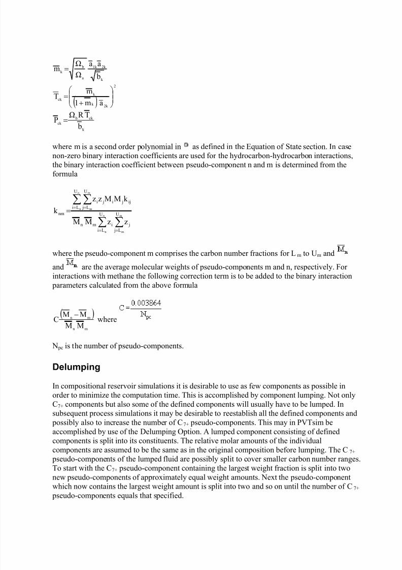
7/18/2019 PVTsim Tutorial Calsep
http://slidepdf.com/reader/full/pvtsim-tutorial-calsep 43/140
k
2k 1k
a
bk
b
aa
Ω
Ωm =
( )
2
2k k
k
ck am1
m
T
+=
k
ck bck b
TR ΩP =
where m is a second order polynomial in as defined in the Equation of State section. In casenon-zero binary interaction coefficients are used for the hydrocarbon-hydrocarbon interactions,the binary interaction coefficient between pseudo-component n and m is determined from theformula
∑ ∑
∑ ∑
= =
= ==n
n
m
m
n
n
m
m
U
Li
U
L j jimn
U
Li
U
L jij ji ji
nm
zzMM
k MMzzk
where the pseudo-component m comprises the carbon number fractions for Lm to Um and
and are the average molecular weights of pseudo-components m and n, respectively. Forinteractions with methane the following correction term is to be added to the binary interaction
parameters calculated from the above formula
( )mn MM
mn MMC
−
where
N pc is the number of pseudo-components.
Delumping
In compositional reservoir simulations it is desirable to use as few components as possible in
order to minimize the computation time. This is accomplished by component lumping. Not onlyC7+ components but also some of the defined components will usually have to be lumped. Insubsequent process simulations it may be desirable to reestablish all the defined components and
possibly also to increase the number of C7+ pseudo-components. This may in PVTsim beaccomplished by use of the Delumping Option. A lumped component consisting of definedcomponents is split into its constituents. The relative molar amounts of the individualcomponents are assumed to be the same as in the original composition before lumping. The C7+
pseudo-components of the lumped fluid are possibly split to cover smaller carbon number ranges.To start with the C7+ pseudo-component containing the largest weight fraction is split into twonew pseudo-components of approximately equal weight amounts. Next the pseudo-componentwhich now contains the largest weight amount is split into two and so on until the number of C7+
pseudo-components equals that specified.
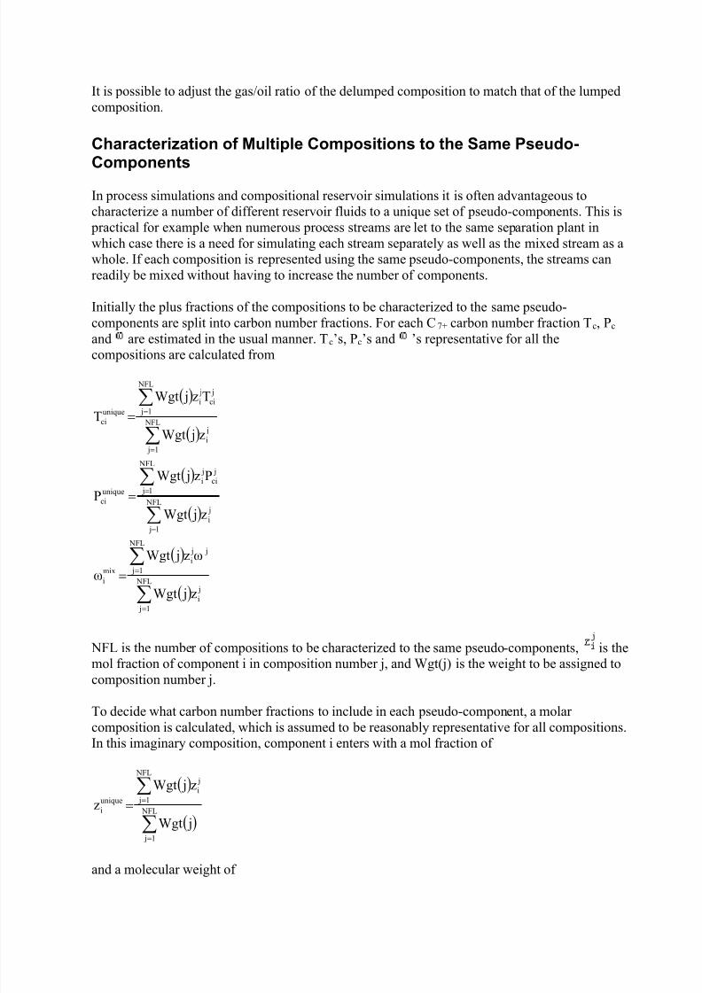
7/18/2019 PVTsim Tutorial Calsep
http://slidepdf.com/reader/full/pvtsim-tutorial-calsep 44/140
It is possible to adjust the gas/oil ratio of the delumped composition to match that of the lumpedcomposition.
Characterization of Multiple Compositions to the Same Pseudo-
ComponentsIn process simulations and compositional reservoir simulations it is often advantageous tocharacterize a number of different reservoir fluids to a unique set of pseudo-components. This is
practical for example when numerous process streams are let to the same separation plant inwhich case there is a need for simulating each stream separately as well as the mixed stream as awhole. If each composition is represented using the same pseudo-components, the streams canreadily be mixed without having to increase the number of components.
Initially the plus fractions of the compositions to be characterized to the same pseudo-components are split into carbon number fractions. For each C7+ carbon number fraction Tc, Pc
and are estimated in the usual manner. Tc’s, Pc’s and ’s representative for all thecompositions are calculated from
( )
( )∑
∑
=
== NFL
1 j
ji
NFL
1 j
jci
ji
uniqueci
z jWgt
Tz jWgt
T
( )
( )∑
∑
=
== NFL
1 j
ji
NFL
1 j
jci
ji
uniqueci
z jWgt
Pz jWgt
P
( )
( )∑
∑
=
== NFL
1 j
ji
NFL
1 j
j ji
mixi
z jWgt
ωz jWgt
ω
NFL is the number of compositions to be characterized to the same pseudo-components, is themol fraction of component i in composition number j, and Wgt(j) is the weight to be assigned to
composition number j.
To decide what carbon number fractions to include in each pseudo-component, a molarcomposition is calculated, which is assumed to be reasonably representative for all compositions.In this imaginary composition, component i enters with a mol fraction of
( )
( )∑
∑
=
== NFL
1 j
NFL
1 j
ji
uniquei
jWgt
z jWgt
z
and a molecular weight of
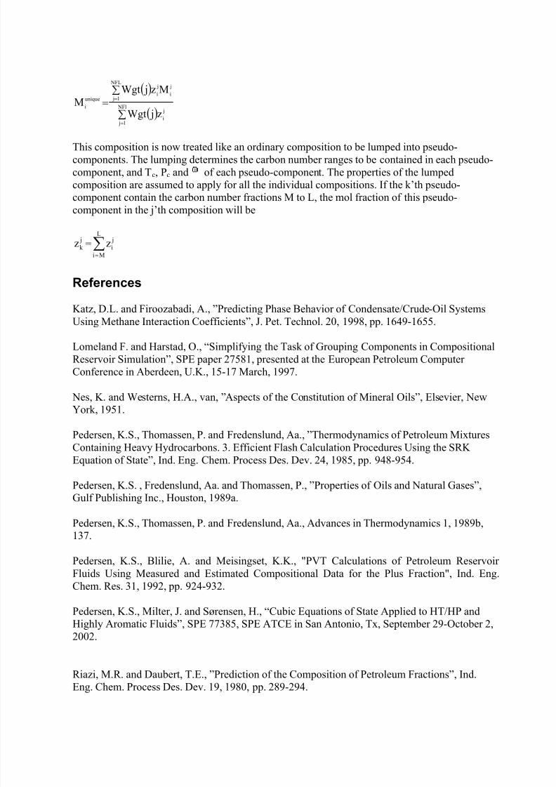
7/18/2019 PVTsim Tutorial Calsep
http://slidepdf.com/reader/full/pvtsim-tutorial-calsep 45/140
( )
( )∑
∑=
=
=
NFl
1 j
j
i
j
i
NFL
1 j
j
iunique
i
z jWgt
Mz jWgtM
This composition is now treated like an ordinary composition to be lumped into pseudo-components. The lumping determines the carbon number ranges to be contained in each pseudo-component, and Tc, Pc and of each pseudo-component. The properties of the lumpedcomposition are assumed to apply for all the individual compositions. If the k’th pseudo-component contain the carbon number fractions M to L, the mol fraction of this pseudo-component in the j’th composition will be
∑=
=L
Mi
ji
jk zz
References
Katz, D.L. and Firoozabadi, A., ”Predicting Phase Behavior of Condensate/Crude-Oil SystemsUsing Methane Interaction Coefficients”, J. Pet. Technol. 20, 1998, pp. 1649-1655.
Lomeland F. and Harstad, O., “Simplifying the Task of Grouping Components in CompositionalReservoir Simulation”, SPE paper 27581, presented at the European Petroleum ComputerConference in Aberdeen, U.K., 15-17 March, 1997.
Nes, K. and Westerns, H.A., van, ”Aspects of the Constitution of Mineral Oils”, Elsevier, New
York, 1951.
Pedersen, K.S., Thomassen, P. and Fredenslund, Aa., ”Thermodynamics of Petroleum MixturesContaining Heavy Hydrocarbons. 3. Efficient Flash Calculation Procedures Using the SRKEquation of State”, Ind. Eng. Chem. Process Des. Dev. 24, 1985, pp. 948-954.
Pedersen, K.S. , Fredenslund, Aa. and Thomassen, P., ”Properties of Oils and Natural Gases”,Gulf Publishing Inc., Houston, 1989a.
Pedersen, K.S., Thomassen, P. and Fredenslund, Aa., Advances in Thermodynamics 1, 1989b,137.
Pedersen, K.S., Blilie, A. and Meisingset, K.K., "PVT Calculations of Petroleum ReservoirFluids Using Measured and Estimated Compositional Data for the Plus Fraction", Ind. Eng.Chem. Res. 31, 1992, pp. 924-932.
Pedersen, K.S., Milter, J. and Sørensen, H., “Cubic Equations of State Applied to HT/HP andHighly Aromatic Fluids”, SPE 77385, SPE ATCE in San Antonio, Tx, September 29-October 2,2002.
Riazi, M.R. and Daubert, T.E., ”Prediction of the Composition of Petroleum Fractions”, Ind.Eng. Chem. Process Des. Dev. 19, 1980, pp. 289-294.
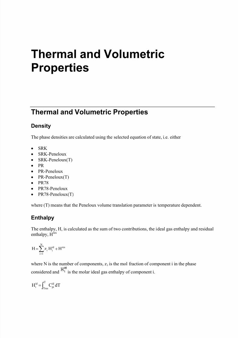
7/18/2019 PVTsim Tutorial Calsep
http://slidepdf.com/reader/full/pvtsim-tutorial-calsep 46/140
Thermal and VolumetricProperties
Thermal and Volumetric Properties
Density
The phase densities are calculated using the selected equation of state, i.e. either
• SRK• SRK-Peneloux• SRK-Peneloux(T)• PR• PR-Peneloux
• PR-Peneloux(T)• PR78• PR78-Peneloux• PR78-Peneloux(T)
where (T) means that the Peneloux volume translation parameter is temperature dependent.
Enthalpy
The enthalpy, H, is calculated as the sum of two contributions, the ideal gas enthalpy and residual
enthalpy, Hres
∑=
+= N
li
residii HHzH
where N is the number of components, zi is the mol fraction of component i in the phase
considered and is the molar ideal gas enthalpy of component i.
∫=T
Tres
id pi
idi dTCH
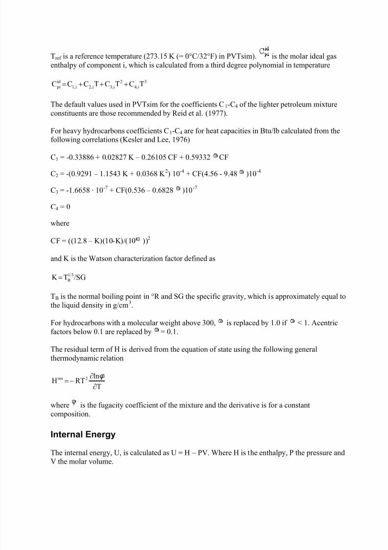
7/18/2019 PVTsim Tutorial Calsep
http://slidepdf.com/reader/full/pvtsim-tutorial-calsep 47/140
Tref is a reference temperature (273.15 K (= 0°C/32°F) in PVTsim). is the molar ideal gasenthalpy of component i, which is calculated from a third degree polynomial in temperature
3i4,
2i3,i2,i1,
id pi TCTCTCCC +++=
The default values used in PVTsim for the coefficients C1-C4 of the lighter petroleum mixtureconstituents are those recommended by Reid et al. (1977).
For heavy hydrocarbons coefficients C1-C4 are for heat capacities in Btu/lb calculated from thefollowing correlations (Kesler and Lee, 1976)
C1 = -0.33886 + 0.02827 K – 0.26105 CF + 0.59332 CF
C2 = -(0.9291 – 1.1543 K + 0.0368 K 2) 10-4 + CF(4.56 - 9.48 )10-4
C3 = -1.6658 · 10-7 + CF(0.536 – 0.6828 )10-7
C4 = 0
where
CF = ((12.8 – K)(10-K)/(10 ))2
and K is the Watson characterization factor defined as
/SGTK 1/3B=
TB is the normal boiling point in °R and SG the specific gravity, which is approximately equal tothe liquid density in g/cm3.
For hydrocarbons with a molecular weight above 300, is replaced by 1.0 if < 1. Acentricfactors below 0.1 are replaced by = 0.1.
The residual term of H is derived from the equation of state using the following generalthermodynamic relation
TlnRTH 2res
∂∂−=
where is the fugacity coefficient of the mixture and the derivative is for a constantcomposition.
Internal Energy
The internal energy, U, is calculated as U = H – PV. Where H is the enthalpy, P the pressure andV the molar volume.
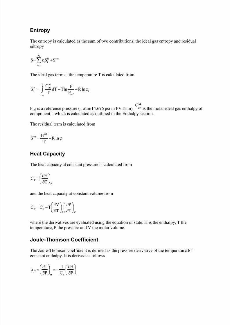
7/18/2019 PVTsim Tutorial Calsep
http://slidepdf.com/reader/full/pvtsim-tutorial-calsep 48/140
Entropy
The entropy is calculated as the sum of two contributions, the ideal gas entropy and residualentropy
∑=
+= N
1i
residii SSzS
The ideal gas term at the temperature T is calculated from
∫ −−=T
T
i
ref
id piid
i
ref
zlnR P
PTlndT
T
CS
Pref is a reference pressure (1 atm/14.696 psi in PVTsim). is the molar ideal gas enthalpy of
component i, which is calculated as outlined in the Enthalpy section.
The residual term is calculated from
ϕ lnR T
HS
ref ref −=
Heat Capacity
The heat capacity at constant pressure is calculated from
PP T
HC
∂∂
=
and the heat capacity at constant volume from
VPPV T
P
T
VTCC
∂∂
∂∂
−=
where the derivatives are evaluated using the equation of state. H is the enthalpy, T thetemperature, P the pressure and V the molar volume.
Joule-Thomson Coefficient
The Joule-Thomson coefficient is defined as the pressure derivative of the temperature forconstant enthalpy. It is derived as follows
T pH jT P
H
C
1
P
Tµ
∂∂
−=
∂∂
=
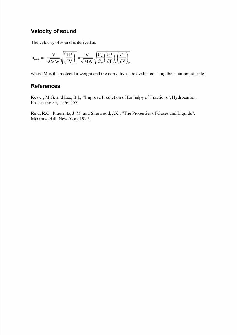
7/18/2019 PVTsim Tutorial Calsep
http://slidepdf.com/reader/full/pvtsim-tutorial-calsep 49/140
Velocity of sound
The velocity of sound is derived as
PVV
P
Ssonic V
T
T
P
C
C
MW
V
V
P
MW
Vu
∂∂
∂∂
=
∂∂
−=
where M is the molecular weight and the derivatives are evaluated using the equation of state.
References
Kesler, M.G. and Lee, B.I., ”Improve Prediction of Enthalpy of Fractions”, HydrocarbonProcessing 55, 1976, 153.
Reid, R.C., Prausnitz, J. M. and Sherwood, J.K., ”The Properties of Gases and Liquids”.McGraw-Hill, New-York 1977.
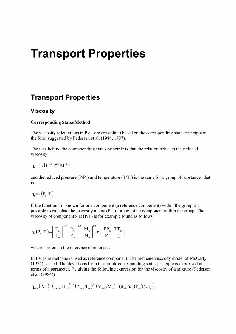
7/18/2019 PVTsim Tutorial Calsep
http://slidepdf.com/reader/full/pvtsim-tutorial-calsep 50/140
Transport Properties
Transport Properties
Viscosity
Corresponding States Method
The viscosity calculations in PVTsim are default based on the corresponding states principle inthe form suggested by Pedersen et al. (1984, 1987).
The idea behind the corresponding states principle is that the relation between the reducedviscosity
( )1/22/3
c
-1/6
cr MPT/ηη =
and the reduced pressure (P/Pc) and temperature (T/Tc) is the same for a group of substances thatis
( )r r r T,Pf η =
If the function f is known for one component (a reference component) within the group it is possible to calculate the viscosity at any (P,T) for any other component within the group. Theviscosity of component x at (P,T) is for example found as follows
( )
=
−
cx
co
cx
coo
1/2
o
x
2/3
co
cx
1/6
co
cxr r x
TTT,
PPPη
MM
PP
TTT,Pη
where o refers to the reference component.
In PVTsim methane is used as reference component. The methane viscosity model of McCarty(1974) is used. The deviations from the simple corresponding states principle is expressed interms of a parameter, , giving the following expression for the viscosity of a mixture (Pedersenet al. (1984))
( ) ( ) ( ) ( ) ( )oooomix
1/2
omix
2/3
comixc,
1/6
comixc,mix T,Pη)/α(α/MM/PP/TTTP,η
−
=
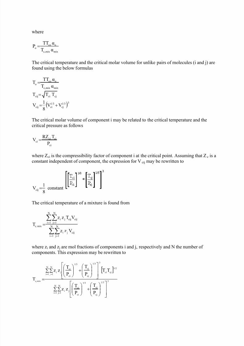
7/18/2019 PVTsim Tutorial Calsep
http://slidepdf.com/reader/full/pvtsim-tutorial-calsep 51/140
where
mixmixc,
ocoo
αT
αTTP =
The critical temperature and the critical molar volume for unlike pairs of molecules (i and j) arefound using the below formulas
mixmixc,
ocoo
αT
αTTT =
cjcicij TTT =
( )31/3cj
1/3cicij VV
8
1V +=
The critical molar volume of component i may be related to the critical temperature and thecritical pressure as follows
ci
cicici P
TRZV =
where Zci is the compressibility factor of component i at the critical point. Assuming that Zc is aconstant independent of component, the expression for Vcij may be rewritten to
8
1Vcij = constant
The critical temperature of a mixture is found from
∑∑
∑∑
= =
= == N
1i
N
1 jcij ji
N
1i
N
1 jcijcij ji
mixc,
Vzz
VTzz
T
where zi and z j are mol fractions of components i and j, respectively and N the number ofcomponents. This expression may be rewritten to
[ ]
∑
+
∑
∑∑
+
=
= =
= =
N
1i
31/3
cj
cj
1/3
ci
ci N
1 j ji
N
1i
N
1 j
1/2
cjci
31/3
cj
cj
1/3
ci
ci ji
mixc,
P
T
P
Tzz
TTP
T
P
Tzz
T
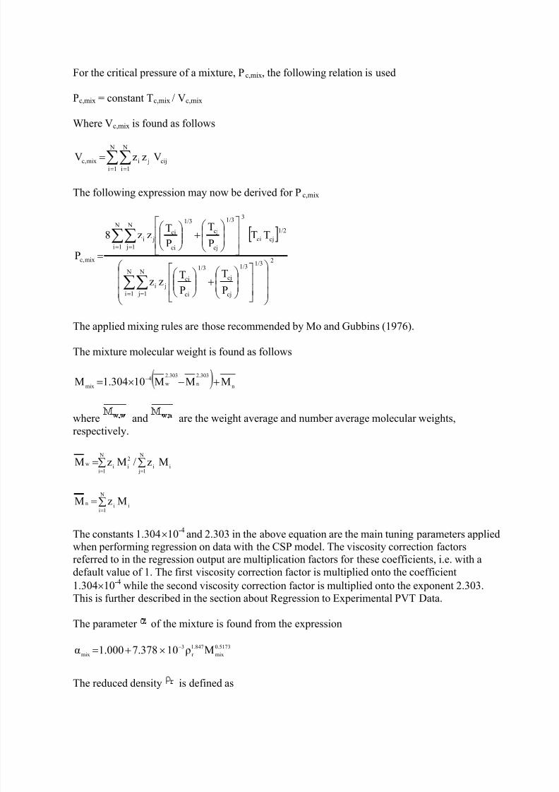
7/18/2019 PVTsim Tutorial Calsep
http://slidepdf.com/reader/full/pvtsim-tutorial-calsep 52/140
For the critical pressure of a mixture, Pc,mix, the following relation is used
Pc,mix = constant Tc,mix / Vc,mix
Where Vc,mix is found as follows
∑∑= =
= N
1i
N
1icij jimixc, VzzV
The following expression may now be derived for Pc,mix
[ ]
2
N
1i
N
1 j
1/31/3
cj
cj
1/3
ci
ci ji
N
1i
1/2
cjci
3 N
1 j
1/3
cj
cj
1/3
ci
ci ji
mixc,
PT
PTzz
TTP
T
P
Tzz8
P
+
+
=
∑∑
∑∑
= =
= =
The applied mixing rules are those recommended by Mo and Gubbins (1976).
The mixture molecular weight is found as follows
n
2.303
n
2.303
w4
mix MMM101.304M +−×= −
where and are the weight average and number average molecular weights,respectively.
∑ ∑== =
N
1i
N
1 jii
2
iiw Mz/MzM
∑==
N
1iiin MzM
The constants 1.304×10⁻⁴ and 2.303 in the above equation are the main tuning parameters applied
when performing regression on data with the CSP model. The viscosity correction factorsreferred to in the regression output are multiplication factors for these coefficients, i.e. with adefault value of 1. The first viscosity correction factor is multiplied onto the coefficient1.304×10-4 while the second viscosity correction factor is multiplied onto the exponent 2.303.This is further described in the section about Regression to Experimental PVT Data.
The parameter of the mixture is found from the expression
0.5173
mix
1.847
r
3
mix Mρ107.3781.000α −×+=
The reduced density is defined as
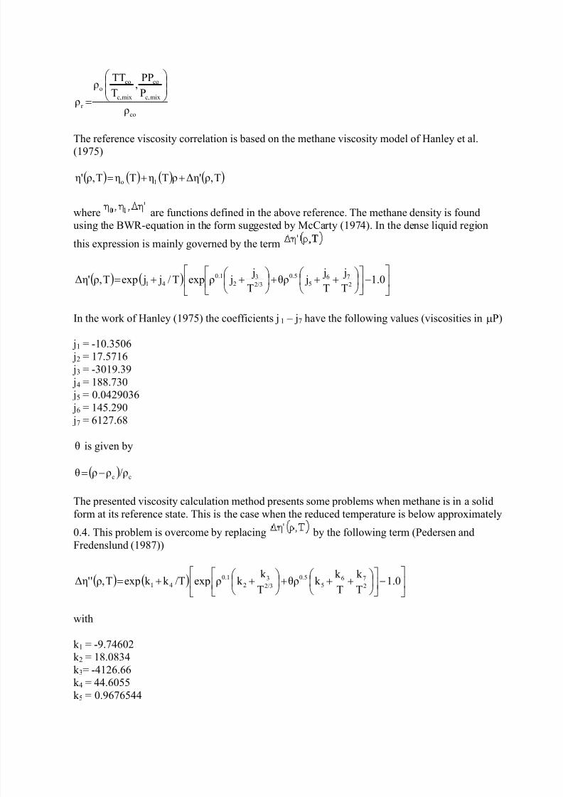
7/18/2019 PVTsim Tutorial Calsep
http://slidepdf.com/reader/full/pvtsim-tutorial-calsep 53/140
co
mixc,
co
mixc,
coo
r ρ
P
PP,
T
TTρ
ρ
=
The reference viscosity correlation is based on the methane viscosity model of Hanley et al.(1975)
( ) ( ) ( ) ( )Tρ,∆η'ρTηTηTρ,η' 1o ++=
where are functions defined in the above reference. The methane density is foundusing the B R-equation in the form suggested by McCarty (1974). In the dense liquid region
ainly governed by the term
W
this expression is m
( ) ( )
−
+++
++= 1.0
T j
T j jθρ
T j jρexpT/ j jexpTρ,∆η' 2
765
0.52/33
20.1
41
In the work of Hanley (1975) the coefficients j1 – j7 have the following values (viscosities in µP)
j1 = -10.3506 j2 = 17.5716 j3 = -3019.39 j4 = 188.730 j5 = 0.0429036
j6 = 145.290 j7 = 6127.68
θ is given by
( ) cc /ρρρθ −=
The presented viscosity calculation method presents some problems when methane is in a solidform at its reference state. This is the case when the reduced temperature is below approximately
0.4. This problem is overcome by replacing by the following term (Pedersen and
Fredenslund (1987))
( ) ( )
−
+++
++= 1.0T
k
T
k k θρ
T
k k ρexp/Tk k expTρ,'∆η'
276
50.5
2/33
20.1
41
with
k 1 = -9.74602k 2 = 18.0834k 3= -4126.66
k 4 = 44.6055k 5 = 0.9676544
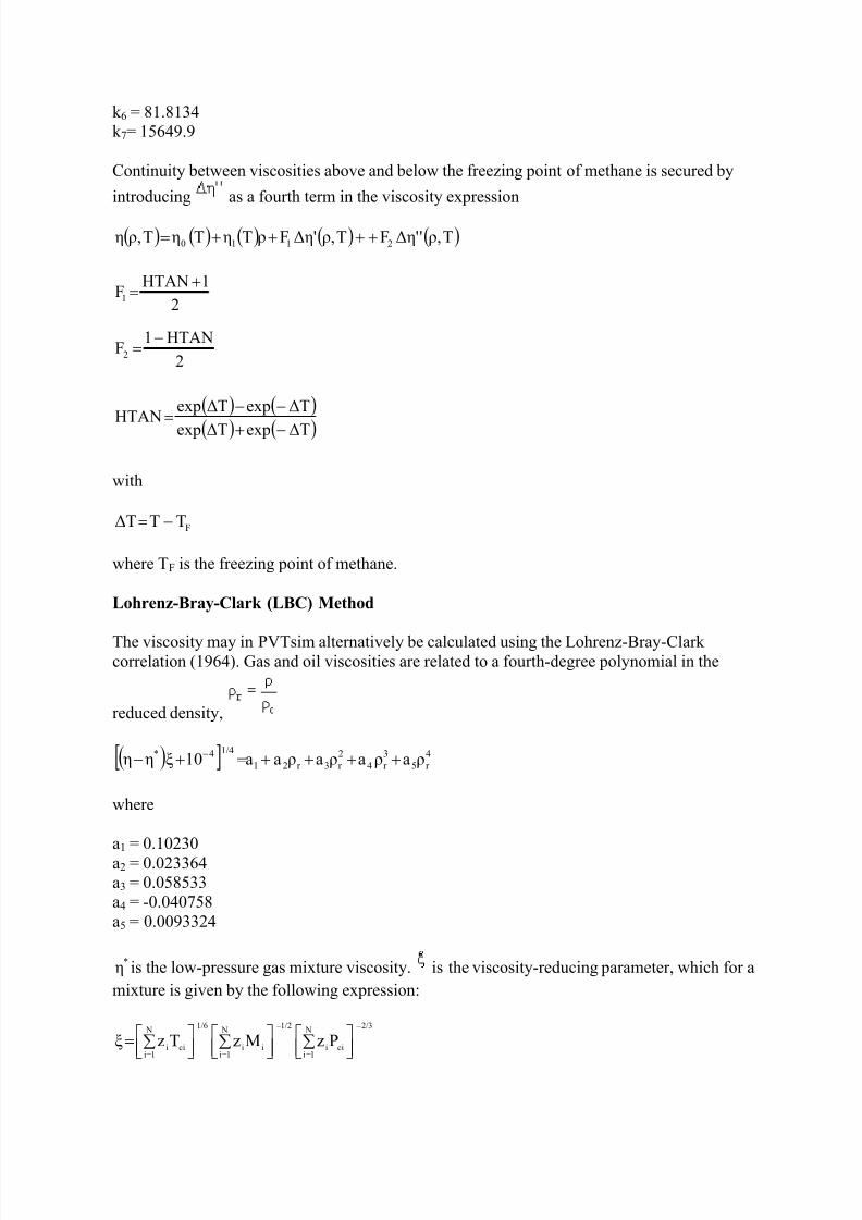
7/18/2019 PVTsim Tutorial Calsep
http://slidepdf.com/reader/full/pvtsim-tutorial-calsep 54/140
k 6 = 81.8134k 7= 15649.9
Continuity between viscosities above and below the freezing point of methane is secured by
introducing as a fourth term in the viscosity expression
( ) ( ) ( ) ( ) ( )Tρ,'∆η'FTρ,∆η'FρTηTηTρ,η 2110 ++++=
2
1HTANF1
+=
2
HTAN1F2
−=
( ) ( )( ) ( )∆Texp∆Texp
∆Texp∆Texp
HTAN −+
−−
=
with
FTT∆T −=
where TF is the freezing point of methane.
Lohrenz-Bray-Clark (LBC) Method
The viscosity may in PVTsim alternatively be calculated using the Lohrenz-Bray-Clarkcorrelation (1964). Gas and oil viscosities are related to a fourth-degree polynomial in the
reduced density,
( )[ ] 4r 5
3r 4
2r 3r 21
1/44* ρaρaρaρaa10ξηη ++++=+− −
where
a1 = 0.10230a2 = 0.023364a3 = 0.058533a4 = -0.040758a5 = 0.0093324
*η is the low-pressure gas mixture viscosity. is the viscosity-reducing parameter, which for a
mixture is given by the following expression:
2/3 N
1i cii
1/2 N
1i ii
1/6 N
1i cii
PzMzTzξ−
=
−
==
∑
∑
∑=
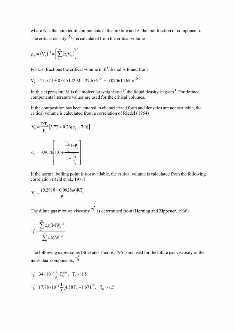
7/18/2019 PVTsim Tutorial Calsep
http://slidepdf.com/reader/full/pvtsim-tutorial-calsep 55/140
where N is the number of components in the mixture and zi the mol fraction of component i.
The critical density, , is calculated from the critical volume
( ) ( )1 N
1icii
1
cc VzVρ
−
=
−
==
∑
For C7+ fractions the critical volume in ft3/lb mol is found from
Vc = 21.573 + 0.015122 M – 27.656 + 0.070615 M ×
In this expression, M is the molecular weight and the liquid density in g/cm3. For definedcomponents literature values are used for the critical volumes.
If the composition has been entered in characterized form and densities are not available, the
critical volume is calculated from a correlation of Riedel (1954)
[ ] 1c
c
cc 7.0)0.26(α3.72
P
RTV −−+=
−+=
c
b
c
c
b
c
T
T1
lnPT
T
1.00.9076α
If the normal boiling point is not available, the critical volume is calculated from the followingcorrelation (Reid et al., 1977)
c
cc P
)RT0.0928(0.2918V
ω −=
The dilute gas mixture viscosity is determined from (Herning and Zippener, 1936)
∑
∑
=
== N
1i
1/2ii
N
1i
1/2i
*ii
*
MWz
MWηz
η
The following expressions (Stiel and Thodos, 1961) are used for the dilute gas viscosity of the
individual components,
1.5T,Tξ
11034η ri
0.94ri
i
5*i <×= −
( ) 1.5T,1.67T4.58ξ
11017.78η ri
5/8
ri5*i >−×= −
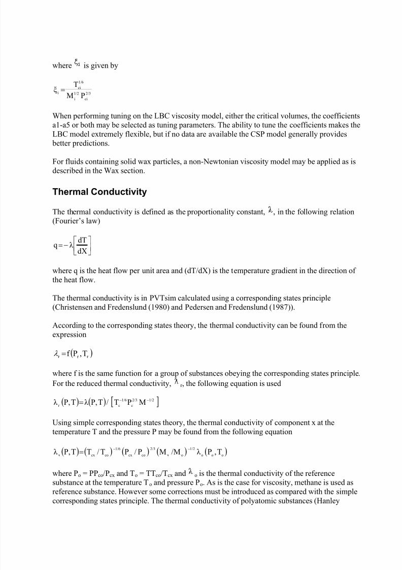
7/18/2019 PVTsim Tutorial Calsep
http://slidepdf.com/reader/full/pvtsim-tutorial-calsep 56/140
where is given by
2/3
ci
1/2
i
1/6
cii
PM
Tξ =
When performing tuning on the LBC viscosity model, either the critical volumes, the coefficientsa1-a5 or both may be selected as tuning parameters. The ability to tune the coefficients makes theLBC model extremely flexible, but if no data are available the CSP model generally provides
better predictions.
For fluids containing solid wax particles, a non-Newtonian viscosity model may be applied as isdescribed in the Wax section.
Thermal Conductivity
The thermal conductivity is defined as the proportionality constant, , in the following relation(Fourier’s law)
−=dX
dTλ q
where q is the heat flow per unit area and (dT/dX) is the temperature gradient in the direction ofthe heat flow.
The thermal conductivity is in PVTsim calculated using a corresponding states principle(Christensen and Fredenslund (1980) and Pedersen and Fredenslund (1987)).
According to the corresponding states theory, the thermal conductivity can be found from theexpression
( )r r r T,Pf =λ
where f is the same function for a group of substances obeying the corresponding states principle.For the reduced thermal conductivity, r , the following equation is used
( ) ( ) [ ]1/22/3
c
1/6
cr MPT/TP,λ TP,λ −−=
Using simple corresponding states theory, the thermal conductivity of component x at thetemperature T and the pressure P may be found from the following equation
( ) ( ) ( ) ( ) ( )ooo
1/2
ox
2/3
cocx
1/6
cocxx T,Pλ /MMP/PT/TTP,λ −−=
where Po = PPco/Pcx and To = TTco/Tcx and o is the thermal conductivity of the referencesubstance at the temperature To and pressure Po. As is the case for viscosity, methane is used as
reference substance. However some corrections must be introduced as compared with the simplecorresponding states principle. The thermal conductivity of polyatomic substances (Hanley
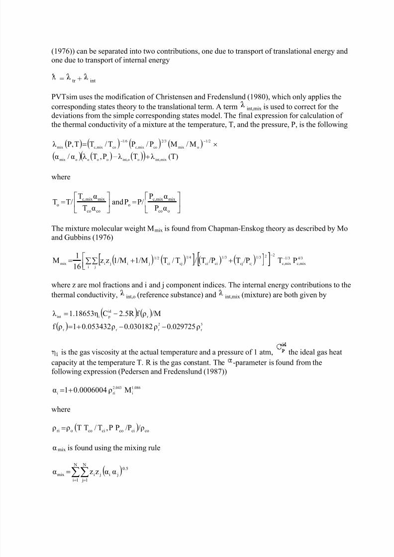
7/18/2019 PVTsim Tutorial Calsep
http://slidepdf.com/reader/full/pvtsim-tutorial-calsep 57/140
(1976)) can be separated into two contributions, one due to transport of translational energy andone due to transport of internal energy
= tr + int
PVTsim uses the modification of Christensen and Fredenslund (1980), which only applies thecorresponding states theory to the translational term. A term int,mix is used to correct for thedeviations from the simple corresponding states model. The final expression for calculation ofthe thermal conductivity of a mixture at the temperature, T, and the pressure, P, is the following
( ) ( ) ( ) ( )
( ) ( ) ( )( ) (T)λ Tλ P,Tλ α/α
M/MP/PT/TTP,λ
mixint,ooint,oooomix
1/2
omix
2/3
comixc,
1/6
comixc,mix
+−
×= −−
where
=
=
oco
mixmixc,o
coco
mixmixc,o
αP
αPP/Pand
αT
αTT/T
The mixture molecular weight Mmix is found from Chapman-Enskog theory as described by Moand Gubbins (1976)
( ) ( )[ ] ( ) ( ) ][ ] 4/3
mixc,
1/3
mixc,
221/3
cjcj
1/3
cicii j
1/4
cjci
1/2
ji jimix PT/PT/PT/T/T1/M1/Mzz16
1M −
−
+∑∑ +=
where z are mol fractions and i and j component indices. The internal energy contributions to thethermal conductivity, int,o (reference substance) and int,mix (mixture) are both given by
( ) ( )
( ) 3
r
2
r r r
r
id
piint
ρ0.029725ρ0.030182ρ0.0534321ρf
/Mρf 2.5R C1.18653ηλ
−−+=
−=
is the gas viscosity at the actual temperature and a pressure of 1 atm, the ideal gas heat
capacity at the temperature T. R is the gas constant. The -parameter is found from thefollowing expression (Pedersen and Fredenslund (1987))
1.086
i
2.043
rii Mρ0.00060041α +=
where
( ) cocicocicoori /ρ/PPP,T/TTρρ =
αmix is found using the mixing rule
( )∑∑= =
= N
1i
N
1 j
0.5
ji jimix ααzzα
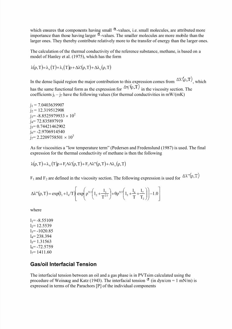
7/18/2019 PVTsim Tutorial Calsep
http://slidepdf.com/reader/full/pvtsim-tutorial-calsep 58/140
which ensures that components having small -values, i.e. small molecules, are attributed moreimportance than those having larger -values. The smaller molecules are more mobile than thelarger ones. They thereby contribute relatively more to the transfer of energy than the larger ones.
The calculation of the thermal conductivity of the reference substance, methane, is based on a
model of Hanley et al. (1975), which has the form
( ) ( ) ( ) ( ) ( )Tρ,∆λ Tρ,∆λ 'ρTλ Tλ Tρ,λ c1o +++=
In the dense liquid region the major contribution to this expression comes from , which
has the same functional form as the expression for in the viscosity section. Thecoefficients ji – j7 have the following values (for thermal conductivities in mW/(mK)
j1 = 7.0403639907 j2 = 12.319512908 j3= -8.8525979933 × 10² j4= 72.835897919 j5= 0.74421462902 j6= -2.9706914540 j7= 2.2209758501 × 10³
As for viscosities a ”low temperature term” (Pedersen and Fredenslund (1987) is used. The finalexpression for the thermal conductivity of methane is then the following
( ) ( ) ( ) ( ) ( )Tρ,∆λ Tρ,'∆λ 'FTρ,∆λ 'FρTλ Tρ,λ c210 +++=
F1 and F2 are defined in the viscosity section. The following expression is used for
( ) ( )
−
+++
++= 1.0T
l
T
llθρ
T
llρexp/TllexpTρ,'∆λ '
2
765
0.5
2/33
20.1
41
where
l1= -8.55109
l2= 12.5539l3= -1020.85l4= 238.394l5= 1.31563l6= -72.5759l7= 1411.60
Gas/oil Interfacial Tension
The interfacial tension between an oil and a gas phase is in PVTsim calculated using the procedure of Weinaug and Katz (1943). The interfacial tension (in dyn/cm = 1 mN/m) isexpressed in terms of the Parachors [P] of the individual components
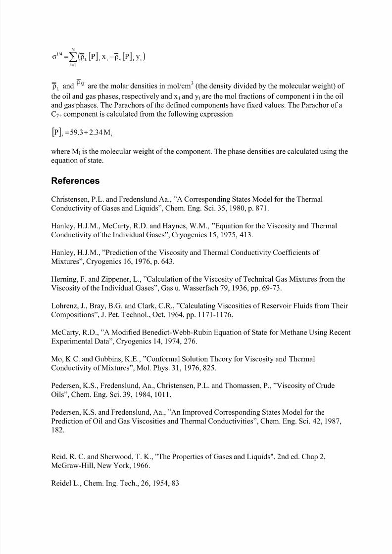
7/18/2019 PVTsim Tutorial Calsep
http://slidepdf.com/reader/full/pvtsim-tutorial-calsep 59/140
[ ] [ ]( )∑=
−= N
1iiiviiL
1/4 yPρxPρσ
Lρ and are the molar densities in mol/cm3 (the density divided by the molecular weight) of
the oil and gas phases, respectively and xi and yi are the mol fractions of component i in the oiland gas phases. The Parachors of the defined components have fixed values. The Parachor of aC7+ component is calculated from the following expression
[ ] ii M2.3459.3P +=
where Mi is the molecular weight of the component. The phase densities are calculated using theequation of state.
References
Christensen, P.L. and Fredenslund Aa., ”A Corresponding States Model for the ThermalConductivity of Gases and Liquids”, Chem. Eng. Sci. 35, 1980, p. 871.
Hanley, H.J.M., McCarty, R.D. and Haynes, W.M., ”Equation for the Viscosity and ThermalConductivity of the Individual Gases”, Cryogenics 15, 1975, 413.
Hanley, H.J.M., ”Prediction of the Viscosity and Thermal Conductivity Coefficients ofMixtures”, Cryogenics 16, 1976, p. 643.
Herning, F. and Zippener, L., ”Calculation of the Viscosity of Technical Gas Mixtures from the
Viscosity of the Individual Gases”, Gas u. Wasserfach 79, 1936, pp. 69-73.
Lohrenz, J., Bray, B.G. and Clark, C.R., ”Calculating Viscosities of Reservoir Fluids from TheirCompositions”, J. Pet. Technol., Oct. 1964, pp. 1171-1176.
McCarty, R.D., ”A Modified Benedict-Webb-Rubin Equation of State for Methane Using RecentExperimental Data”, Cryogenics 14, 1974, 276.
Mo, K.C. and Gubbins, K.E., ”Conformal Solution Theory for Viscosity and ThermalConductivity of Mixtures”, Mol. Phys. 31, 1976, 825.
Pedersen, K.S., Fredenslund, Aa., Christensen, P.L. and Thomassen, P., ”Viscosity of CrudeOils”, Chem. Eng. Sci. 39, 1984, 1011.
Pedersen, K.S. and Fredenslund, Aa., ”An Improved Corresponding States Model for thePrediction of Oil and Gas Viscosities and Thermal Conductivities”, Chem. Eng. Sci. 42, 1987,182.
Reid, R. C. and Sherwood, T. K., "The Properties of Gases and Liquids", 2nd ed. Chap 2,McGraw-Hill, New York, 1966.
Reidel L., Chem. Ing. Tech., 26, 1954, 83
7/18/2019 PVTsim Tutorial Calsep
http://slidepdf.com/reader/full/pvtsim-tutorial-calsep 60/140
Stiel, L. I. and Thodos, G., ”The Viscosity of Non-Polar Gases at Normal Pressures”, AIChE J. 7,1961, pp. 611-615.
Weinaug, C.F. and Katz, D.L., “Surface Tensions of Methane-Propane Mixtures”, Ind. Eng.
Chem. 35, 1943, pp. 239-246.
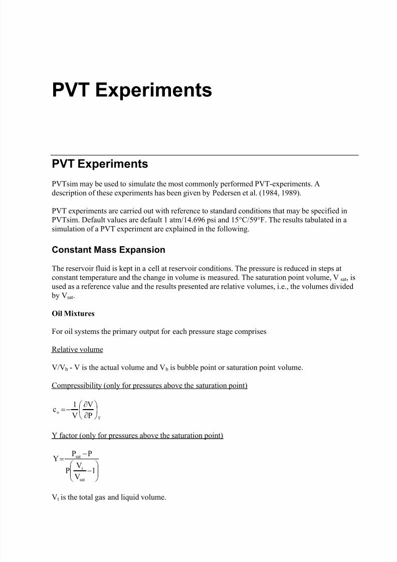
7/18/2019 PVTsim Tutorial Calsep
http://slidepdf.com/reader/full/pvtsim-tutorial-calsep 61/140
PVT Experiments
PVT Experiments
PVTsim may be used to simulate the most commonly performed PVT-experiments. A
description of these experiments has been given by Pedersen et al. (1984, 1989).
PVT experiments are carried out with reference to standard conditions that may be specified inPVTsim. Default values are default 1 atm/14.696 psi and 15°C/59°F. The results tabulated in asimulation of a PVT experiment are explained in the following.
Constant Mass Expansion
The reservoir fluid is kept in a cell at reservoir conditions. The pressure is reduced in steps atconstant temperature and the change in volume is measured. The saturation point volume, Vsat, isused as a reference value and the results presented are relative volumes, i.e., the volumes divided
by Vsat.
Oil Mixtures
For oil systems the primary output for each pressure stage comprises
Relative volume
V/V b - V is the actual volume and V b is bubble point or saturation point volume.
Compressibility (only for pressures above the saturation point)
T
oP
V
V
1c
∂∂
−=
Y factor (only for pressures above the saturation point)
−
−=
1V
VP
PPY
sat
t
sat
Vt is the total gas and liquid volume.
7/18/2019 PVTsim Tutorial Calsep
http://slidepdf.com/reader/full/pvtsim-tutorial-calsep 62/140
Gas Condensate Mixtures
For gas condensate systems the primary output for each pressure stage comprises
Rel Vol V/Vd (Vd is dew point or saturation point volume) Liq Vol Liquid vol% of Vd.Z Factor (only above saturation point)
Differential Depletion
This experiment is only carried out for oil mixtures. The reservoir fluid is kept in a cell at thereservoir temperature. The experiment is usually started at the saturation pressure. The pressureis reduced stepwise and all the liberated gas is displaced and flashed to standard conditions. This
procedure is repeated 6-10 times. The end point is measured at standard conditions.
The primary output for each pressure stage comprises
Oil FVF Oil formation volume factor (Bo) defined as the oil volume atthe actual pressure divided by the residual oil volume atstandard conditions
R sd Solution gas/oil ratio, which is the total standard volume of gasliberated from the oil in the stages to follow, divided by theresidual oil volume. The volume of the liquid condensing whenflashing the gas to standard conditions is converted to anequivalent gas volume.
Gas FVF Gas formation volume factor defined as the volume of the gas atthe actual conditions divided by the volume of the same gas atstandard conditions. The volume of the liquid condensing whenflashing the gas to standard conditions is converted to anequivalent gas volume.
Gas Gravity Molecular weight of the gas divided by the molecular weight ofatmospheric air (=28.964).
Constant Volume Depletion
This experiment is performed for gas condensates and volatile oils.
The reservoir fluid is kept in a cell at reservoir temperature and saturation point pressure. The pressure is reduced in steps, and at each level as much gas is removed that the volume of theremaining gas and oil mixture equals the saturation point volume.
For each pressure stage the primary output consists of
Liq vol Liquid volume% of dew point volume%Prod Cumulative mol% of initial mixture removedZ factor gas
Viscosity Viscosity of the gas in the cell
7/18/2019 PVTsim Tutorial Calsep
http://slidepdf.com/reader/full/pvtsim-tutorial-calsep 63/140
Separator Experiments
Separators in Series
A separator experiment is customarily started at the saturation pressure at the reservoir
temperature. The volume and the density are recorded. Subsequently a series of PT flashseparations is performed. The gas phase from each separator stage is flashed to standardconditions. The liquid phase is let to a new separator in which a new PT flash separation takes
place, and so on. The last separator is at atmospheric conditions.
The primary output consists of
GOR Volume of gas from the actual stage at standard conditions divided bythe volume of the oil from the last stage (atmospheric conditions)
Gas Gravity Molecular weight of the gas divided by the molecular weight of air(28.964)
FVF Oil formation volume factor, which is the oil volume at the actual stagedivided by the oil volume from the last stage.
Sometimes the separator GOR is seen reported as the standard volume of gas divided by theseparator oil volume (oil volume at actual stage). The latter GOR can be converted into thatreported by PVTsim by dividing it by FVF.
Separator Test with Recirculation
PVTsim has an option for simulating a special two stage separator set-up. The gas stream from
the first separator is separated in a second separator. The liquid stream from the second separatoris mixed into the feed to the first separator. The product streams are the liquid stream from thefirst separator and the gas stream from the second separator.
Viscosity Experiment
A viscosity experiment is performed at the reservoir temperature. The pressure is reduced insteps as in a differential depletion experiment. At each step the phase viscosities are recorded.
Swelling Experiment
When gas is injected into a reservoir containing undersaturated oil, the gas may dissolve in theoil. The volume of the oil increases, which is also called swelling. A swelling test experimentmay simulate this process. The cell initially contains reservoir oil. A known molar amount of agas is added at a constant temperature. The saturation pressure of the swollen mixture and thevolume at the saturation point divided by the volume of the original reservoir oil are recorded.More gas is added. The new saturation pressure and saturation point volume are recorded and soon. The primary output consists of
Mol% Cumulative mol% of gas addedGOR Std. volume of gas added per volume of original reservoir fluid
Sat P Saturation pressure after gas injectionSwollen volume Volume of the mixture per volume original reservoir fluid
7/18/2019 PVTsim Tutorial Calsep
http://slidepdf.com/reader/full/pvtsim-tutorial-calsep 64/140
Density Density of swollen mixture at saturation point
It is further indicated in the output whether the saturation point is a bubble point (P b) or a dew point (Pd).
References
Pedersen, K.S., Thomassen, P. and Fredenslund, Aa., ”Thermodynamics of Petroleum MixturesContaining Heavy Hydrocarbons. 3. Efficient Flash Calculation Procedures Using the SRKEquation of State”, Ind. Eng. Chem. Process Des. Dev. 24, 1985, pp. 948-954.
Pedersen, KS., Fredenslund Aa. and Thomassen, P., ”Properties of Oils and Natural Gases”, GulfPublishing Company, Houston, 1989.
Compositional Variation due toGravity
Compositional Variation due to Gravity
Hydrocarbon reservoirs show variations in the composition in the direction from the top to the bottom of the reservoir. The mol fractions of the lighter components decrease, whereas the molfractions of the heavier components increase. This is at least partly explained by the fact that
gravity forces introduce a compositional gradient.
The Depth Gradient options of PVTsim consider
- Isothermal reservoirs- Reservoirs with a vertical temperature gradient.
In the first case temperature is assumed constant over the entire fluid coloumn and thecompositional variations with depth are assumed only to originate from the effect of gravitationalforces. In the second case temperature varies over the fluid coloumn and compositional variationswith depth are affected both by the temperature gradient and by the gravitational forces.
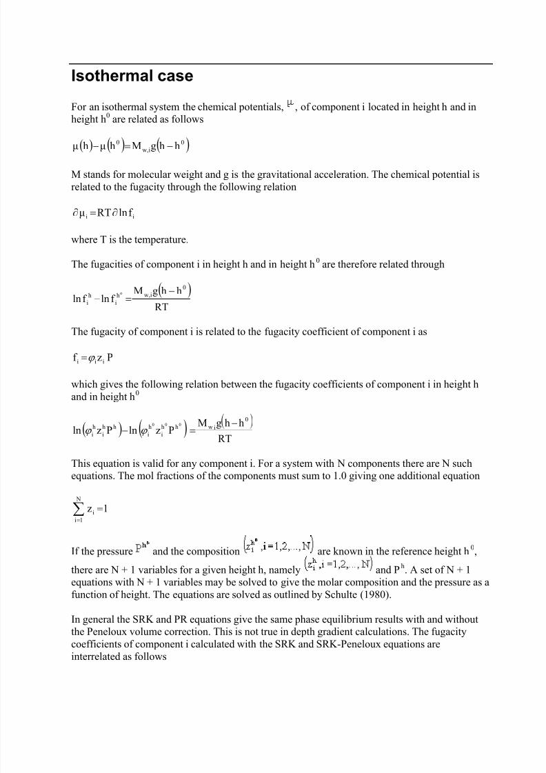
7/18/2019 PVTsim Tutorial Calsep
http://slidepdf.com/reader/full/pvtsim-tutorial-calsep 65/140
Isothermal case
For an isothermal system the chemical potentials, , of component i located in height h and inheight h0 are related as follows
( ) ( ) ( )0w,i
0 hhgMhµhµ −=−
M stands for molecular weight and g is the gravitational acceleration. The chemical potential isrelated to the fugacity through the following relation
ii f lnRTµ ∂=∂
where T is the temperature.
The fugacities of component i in height h and in height h0
are therefore related through
( )RT
hhgMf lnf ln
0w,ih
ih
i
o −=−
The fugacity of component i is related to the fugacity coefficient of component i as
Pzf iii ϕ =
which gives the following relation between the fugacity coefficients of component i in height h
and in height h0
( ) ( )RT
hhgMPzlnPzln
0iwhh
ihi
hhi
hi
000 −=− ϕ ϕ
This equation is valid for any component i. For a system with N components there are N suchequations. The mol fractions of the components must sum to 1.0 giving one additional equation
∑=
= N
1ii 1z
If the pressure and the composition are known in the reference height h0,
there are N + 1 variables for a given height h, namely and Ph. A set of N + 1equations with N + 1 variables may be solved to give the molar composition and the pressure as afunction of height. The equations are solved as outlined by Schulte (1980).
In general the SRK and PR equations give the same phase equilibrium results with and withoutthe Peneloux volume correction. This is not true in depth gradient calculations. The fugacitycoefficients of component i calculated with the SRK and SRK-Peneloux equations areinterrelated as follows
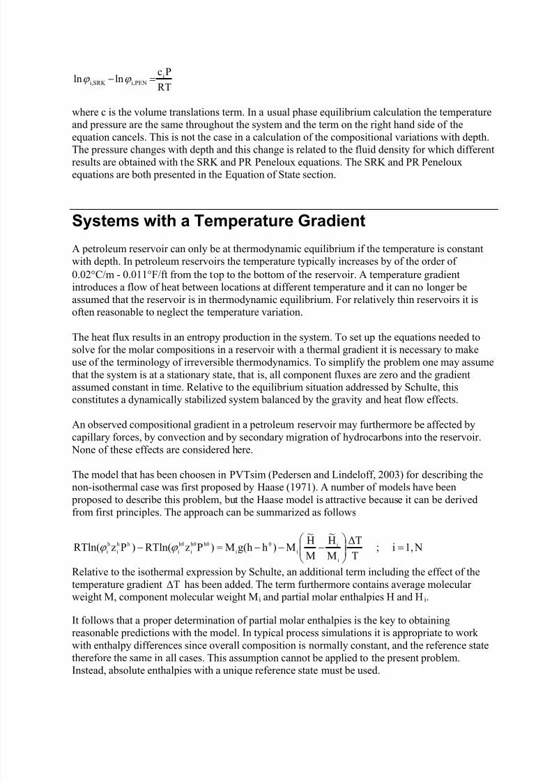
7/18/2019 PVTsim Tutorial Calsep
http://slidepdf.com/reader/full/pvtsim-tutorial-calsep 66/140
RT
Pclnln i
PENi,SRK i, =− ϕ ϕ
where c is the volume translations term. In a usual phase equilibrium calculation the temperatureand pressure are the same throughout the system and the term on the right hand side of the
equation cancels. This is not the case in a calculation of the compositional variations with depth.The pressure changes with depth and this change is related to the fluid density for which differentresults are obtained with the SRK and PR Peneloux equations. The SRK and PR Penelouxequations are both presented in the Equation of State section.
Systems with a Temperature Gradient
A petroleum reservoir can only be at thermodynamic equilibrium if the temperature is constantwith depth. In petroleum reservoirs the temperature typically increases by of the order of0.02°C/m - 0.011°F/ft from the top to the bottom of the reservoir. A temperature gradientintroduces a flow of heat between locations at different temperature and it can no longer beassumed that the reservoir is in thermodynamic equilibrium. For relatively thin reservoirs it isoften reasonable to neglect the temperature variation.
The heat flux results in an entropy production in the system. To set up the equations needed tosolve for the molar compositions in a reservoir with a thermal gradient it is necessary to makeuse of the terminology of irreversible thermodynamics. To simplify the problem one may assumethat the system is at a stationary state, that is, all component fluxes are zero and the gradientassumed constant in time. Relative to the equilibrium situation addressed by Schulte, this
constitutes a dynamically stabilized system balanced by the gravity and heat flow effects.
An observed compositional gradient in a petroleum reservoir may furthermore be affected bycapillary forces, by convection and by secondary migration of hydrocarbons into the reservoir.
None of these effects are considered here.
The model that has been choosen in PVTsim (Pedersen and Lindeloff, 2003) for describing thenon-isothermal case was first proposed by Haase (1971). A number of models have been
proposed to describe this problem, but the Haase model is attractive because it can be derivedfrom first principles. The approach can be summarized as follows
N1,i;T∆T
MH~
MH~M)hg(hM)PzRTln()PzRTln(
i
ii
0
i
h0h0
i
h0
i
hh
i
h
i =
−−−=− ϕ ϕ
Relative to the isothermal expression by Schulte, an additional term including the effect of thetemperature gradient has been added. The term furthermore contains average molecularweight M, component molecular weight M
∆Ti and partial molar enthalpies H and Hi.
It follows that a proper determination of partial molar enthalpies is the key to obtainingreasonable predictions with the model. In typical process simulations it is appropriate to workwith enthalpy differences since overall composition is normally constant, and the reference statetherefore the same in all cases. This assumption cannot be applied to the present problem.
Instead, absolute enthalpies with a unique reference state must be used.
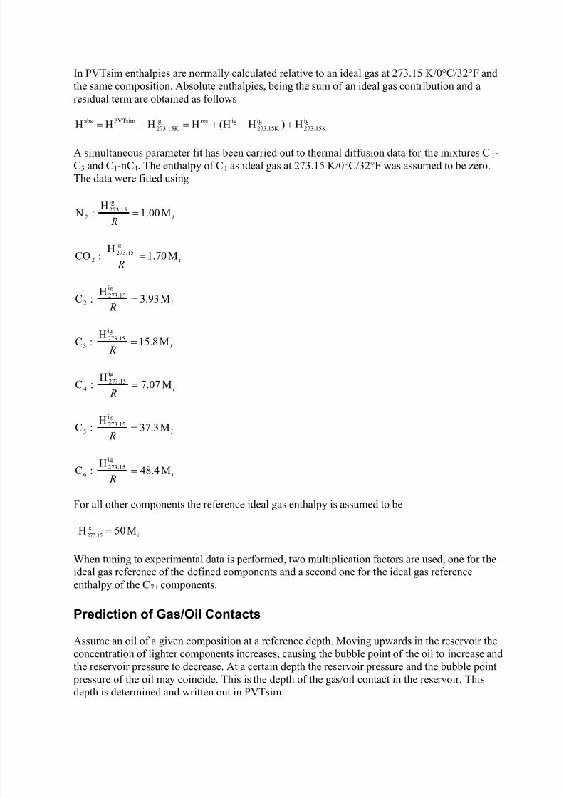
7/18/2019 PVTsim Tutorial Calsep
http://slidepdf.com/reader/full/pvtsim-tutorial-calsep 67/140
In PVTsim enthalpies are normally calculated relative to an ideal gas at 273.15 K/0°C/32°F andthe same composition. Absolute enthalpies, being the sum of an ideal gas contribution and aresidual term are obtained as follows
ig273.15K
ig273.15K
igresig273.15K
PVTsimabs H)H(HHHHH +−+=+=
A simultaneous parameter fit has been carried out to thermal diffusion data for the mixtures C1-C3 and C1-nC4. The enthalpy of C1 as ideal gas at 273.15 K/0°C/32°F was assumed to be zero.The data were fitted using
i R
M00.1H
: Nig273.15
2 =
i R
M1.70H
:COig273.15
2 =
i R
M.933H
:Cig273.15
2 =
i R
M15.8H
:Cig273.15
3 =
i R
M7.07H
:Cig273.15
4 =
i R
M.337H
:Cig273.15
5 =
i R
M.448H
:Cig273.15
6 =
For all other components the reference ideal gas enthalpy is assumed to be
iM50H ig
273.15 =
When tuning to experimental data is performed, two multiplication factors are used, one for theideal gas reference of the defined components and a second one for the ideal gas referenceenthalpy of the C7+ components.
Prediction of Gas/Oil Contacts
Assume an oil of a given composition at a reference depth. Moving upwards in the reservoir theconcentration of lighter components increases, causing the bubble point of the oil to increase andthe reservoir pressure to decrease. At a certain depth the reservoir pressure and the bubble point
pressure of the oil may coincide. This is the depth of the gas/oil contact in the reservoir. Thisdepth is determined and written out in PVTsim.
7/18/2019 PVTsim Tutorial Calsep
http://slidepdf.com/reader/full/pvtsim-tutorial-calsep 68/140
References
Haase, R., Borgmann, H.-W., Dücker, K. H. and Lee, W. P., "Thermodiffusion im kritischenVerdampfungsgebiet Binärer Systeme", Z. Naturforch. 26 a, 1971, pp. 1224-1227.
Schulte, A.M., ”Compositional Variations within a Hydrocarbon Column due to Gravity”, paperSPE 9235 presented at the 1980 SPE Annual Technical Conference and Exhibition Dallas, Sept.21-24, 1980.
Pedersen, K.S. and Lindeloff, N., “Simulations of Compositional Gradients in HydrocarbonReservoirs Under the Influence of a Temperature Gradient”, SPE Paper 84364, to be presented atthe SPE ATCE in Denver, 5-8 October, 2003.
Rutherford, W.M. and Roof, J.G., "Thermal diffusion in methane n-butane mixtures in the criticalregion", J. Phys. Chem. 63, 1959, pp. 1506-1511.
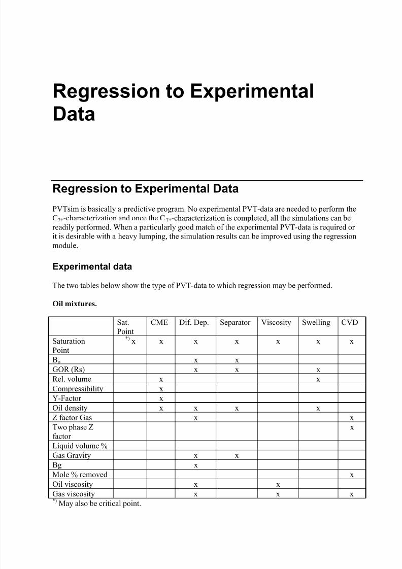
7/18/2019 PVTsim Tutorial Calsep
http://slidepdf.com/reader/full/pvtsim-tutorial-calsep 69/140
Regression to ExperimentalData
Regression to Experimental Data
PVTsim is basically a predictive program. No experimental PVT-data are needed to perform theC7+-characterization and once the C7+-characterization is completed, all the simulations can bereadily performed. When a particularly good match of the experimental PVT-data is required orit is desirable with a heavy lumping, the simulation results can be improved using the regressionmodule.
Experimental data
The two tables below show the type of PVT-data to which regression may be performed.
Oil mixtures.
Sat.Point
CME Dif. Dep. Separator Viscosity Swelling CVD
SaturationPoint
*) x x x x x x x
Bo x xGOR (Rs) x x xRel. volume x x
Compressibility xY-Factor xOil density x x x xZ factor Gas x xTwo phase Zfactor
x
Liquid volume %Gas Gravity x xBg xMole % removed xOil viscosity x xGas viscosity x x x*) May also be critical point.
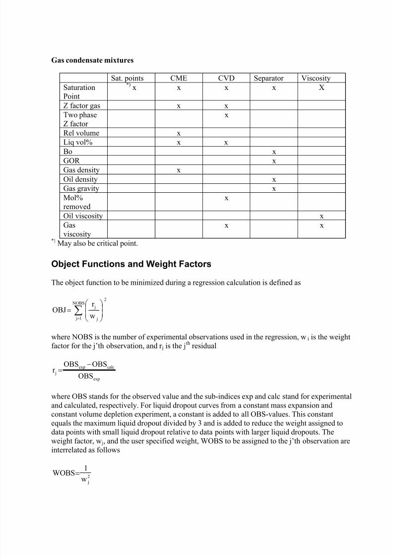
7/18/2019 PVTsim Tutorial Calsep
http://slidepdf.com/reader/full/pvtsim-tutorial-calsep 70/140
Gas condensate mixtures
Sat. points CME CVD Separator ViscositySaturation
Point
*) x x x x X
Z factor gas x xTwo phaseZ factor
x
Rel volume xLiq vol% x xBo xGOR xGas density xOil density x
Gas gravity xMol%removed
x
Oil viscosity xGasviscosity
x x
*) May also be critical point.
Object Functions and Weight Factors
The object function to be minimized during a regression calculation is defined as
∑=
=
NOBS
1 j
2
j
j
w
r OBJ
where NOBS is the number of experimental observations used in the regression, wi is the weightfactor for the j’th observation, and r j is the jth residual
exp
calcexp j OBS
OBSOBSr
−=
where OBS stands for the observed value and the sub-indices exp and calc stand for experimentaland calculated, respectively. For liquid dropout curves from a constant mass expansion andconstant volume depletion experiment, a constant is added to all OBS-values. This constantequals the maximum liquid dropout divided by 3 and is added to reduce the weight assigned todata points with small liquid dropout relative to data points with larger liquid dropouts. Theweight factor, w j, and the user specified weight, WOBS to be assigned to the j’th observation areinterrelated as follows
2 jw
1WOBS=
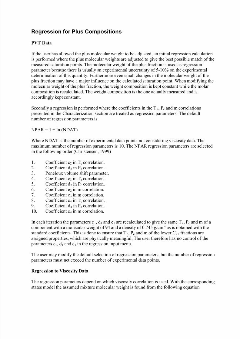
7/18/2019 PVTsim Tutorial Calsep
http://slidepdf.com/reader/full/pvtsim-tutorial-calsep 71/140
Regression for Plus Compositions
PVT Data
If the user has allowed the plus molecular weight to be adjusted, an initial regression calculation
is performed where the plus molecular weights are adjusted to give the best possible match of themeasured saturation points. The molecular weight of the plus fraction is used as regression
parameter because there is usually an experimental uncertainty of 5-10% on the experimentaldetermination of this quantity. Furthermore even small changes in the molecular weight of the
plus fraction may have a major influence on the calculated saturation point. When modifying themolecular weight of the plus fraction, the weight composition is kept constant while the molarcomposition is recalculated. The weight composition is the one actually measured and isaccordingly kept constant.
Secondly a regression is performed where the coefficients in the Tc, Pc and m correlations presented in the Characterization section are treated as regression parameters. The defaultnumber of regression parameters is
NPAR = 1 + ln (NDAT)
Where NDAT is the number of experimental data points not considering viscosity data. Themaximum number of regression parameters is 10. The NPAR regression parameters are selectedin the following order (Christensen, 1999)
1. Coefficient c2 in Tc correlation.2. Coefficient d2 in Pc correlation.
3. Peneloux volume shift parameter.4. Coefficient c3 in Tc correlation.5. Coefficient d3 in Pc correlation.6. Coefficient e2 in m correlation.7. Coefficient e3 in m correlation.8. Coefficient c4 in Tc correlation.9. Coefficient d4 in Pc correlation.10. Coefficient e4 in m correlation.
In each iteration the parameters c1, d1 and e1 are recalculated to give the same Tc, Pc and m of acomponent with a molecular weight of 94 and a density of 0.745 g/cm3 as is obtained with the
standard coefficients. This is done to ensure that Tc, Pc and m of the lower C7+ fractions areassigned properties, which are physically meaningful. The user therefore has no control of the parameters c1, d1 and e1 in the regression input menu.
The user may modify the default selection of regression parameters, but the number of regression parameters must not exceed the number of experimental data points.
Regression to Viscosity Data
The regression parameters depend on which viscosity correlation is used. With the correspondingstates model the assumed mixture molecular weight is found from the following equation
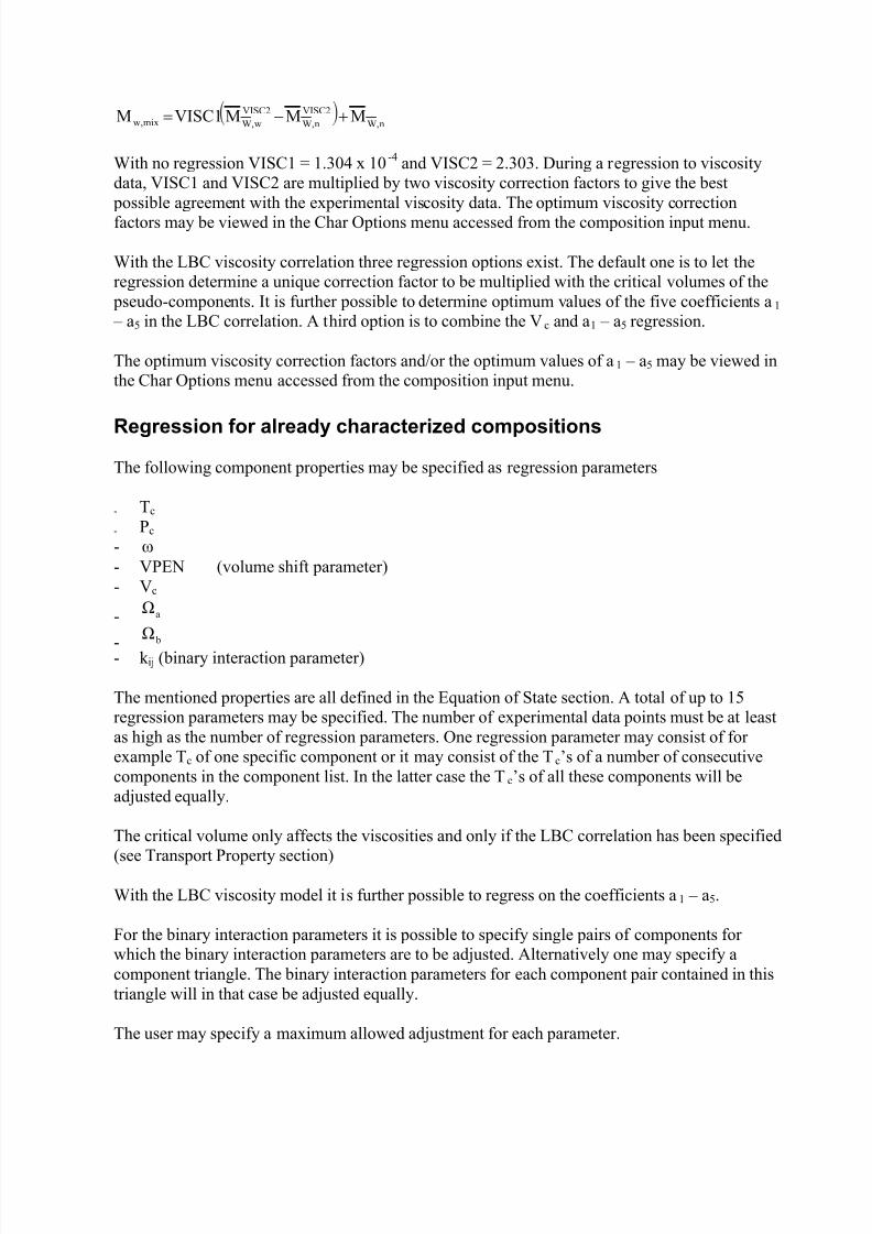
7/18/2019 PVTsim Tutorial Calsep
http://slidepdf.com/reader/full/pvtsim-tutorial-calsep 72/140
n,W
VISC2
n,W
VISC2
w,Wmixw, MMMVISC1M +−=
With no regression VISC1 = 1.304 x 10⁻⁴ and VISC2 = 2.303. During a regression to viscositydata, VISC1 and VISC2 are multiplied by two viscosity correction factors to give the best
possible agreement with the experimental viscosity data. The optimum viscosity correctionfactors may be viewed in the Char Options menu accessed from the composition input menu.
With the LBC viscosity correlation three regression options exist. The default one is to let theregression determine a unique correction factor to be multiplied with the critical volumes of the
pseudo-components. It is further possible to determine optimum values of the five coefficients a1 – a5 in the LBC correlation. A third option is to combine the Vc and a1 – a5 regression.
The optimum viscosity correction factors and/or the optimum values of a1 – a5 may be viewed inthe Char Options menu accessed from the composition input menu.
Regression for already characterized compositions
The following component properties may be specified as regression parameters
- Tc
- Pc
- ω
- VPEN (volume shift parameter)- Vc
- aΩ
- bΩ- k ij (binary interaction parameter)
The mentioned properties are all defined in the Equation of State section. A total of up to 15regression parameters may be specified. The number of experimental data points must be at leastas high as the number of regression parameters. One regression parameter may consist of forexample Tc of one specific component or it may consist of the Tc’s of a number of consecutivecomponents in the component list. In the latter case the Tc’s of all these components will beadjusted equally.
The critical volume only affects the viscosities and only if the LBC correlation has been specified
(see Transport Property section)
With the LBC viscosity model it is further possible to regress on the coefficients a1 – a5.
For the binary interaction parameters it is possible to specify single pairs of components forwhich the binary interaction parameters are to be adjusted. Alternatively one may specify acomponent triangle. The binary interaction parameters for each component pair contained in thistriangle will in that case be adjusted equally.
The user may specify a maximum allowed adjustment for each parameter.
7/18/2019 PVTsim Tutorial Calsep
http://slidepdf.com/reader/full/pvtsim-tutorial-calsep 73/140
Regression on fluids characterized to the same pseudo-components
It is possible to perform regression on fluids which has been characterized to the same set of pseudo-components. This feature can be very powerful, for instance when data are only availablefor some fluid samples. Consider a regression to the same pseudos in a case where data is
available say for 2 fluids out of 5 fluids to be characterized to the same pseudo-components. Inthis case the regression procedure will modify the properties of all 5 fluids while honoring the
best possible match of the available data sets for the two fluids.
Regression Algorithm
The minimization algorithm used in the parameter regression is a Marquardt algorithm(Marquardt, 1963).
References
Christensen, P.L., ”Regression to Experimental PVT Data”, Journal of Canadian PetroleumTechnology 38. 1999, pp. 1-9.
Marquardt, D.W., SIAM J 11 1963, 431-441.
7/18/2019 PVTsim Tutorial Calsep
http://slidepdf.com/reader/full/pvtsim-tutorial-calsep 74/140
Minimum Miscibility PressureCalculations
Minimum Miscibility Pressure Calculations
Injection of gas into oil fields is commonly used to enhance the recovery from the field. Theinjected gas influences the reservoir oil in several ways. It reduces the pressure drop associatedwith the production, it influences the phase properties (density, viscosity, etc.) and it influencesthe gas/oil phase equilibrium. The gas may take up components from the oil phase (vaporizingmechanism), the oil may take up components from the gas phase (condensing mechanism) or theoil and the gas may exhibit first contact miscibility. This means that only one phase is formed, nomatter in what proportion the oil and the gas are mixed. If the gas and the oil are not miscible byfirst contact, miscibility may take place as a result of multiple contacts between the oil and thegas. A miscible gas is advantageous, because valuable heavy components will be contained in a
phase of a fairly high mobility. The mobility is inversely proportional to the viscosity and theviscosity decreases when the oil takes up gaseous components.
With a vaporizing drive, miscibility is achieved at the oil/gas front. At the injection well, bothgas and liquid are present at equilibrium. Compared to the injection gas, the gas phase that has
been in contact with oil contains more intermediate molecular weight components, extractedfrom the oil phase. The gas phase has a higher mobility than the oil phase. Hence, gas which hastaken up intermediate molecular weight components will move forwards and contact originalreservoir oil. With the increasing content of intermediate molecular weight components in the gas
phase, miscibility may be achieved in some distance from the injection well.
In case of a condensing drive, the original reservoir fluid and the injection gas are not miscible, but miscibility may be achieved later on at the injection well. The reservoir fluid takes upintermediate molecular weight components from the injection gas. Since the liquid phase has alower mobility than the gas phase, liquid which has taken up intermediate molecular weightcomponents will be contacted by injection gas. Further transfer of intermediate molecular weightcomponents from the gas to the liquid phase may then occur. After some time, miscibility may beobtained between the injection gas and the liquid phase at the injection well.
Minimum Miscibility Pressure Calculations
The degree of miscibility between a reservoir oil and an injection gas is often expressed in termsof the minimum miscibility pressure (MMP). The first contact minimum miscibility pressure
7/18/2019 PVTsim Tutorial Calsep
http://slidepdf.com/reader/full/pvtsim-tutorial-calsep 75/140
(FCMMP) is the lowest pressure at which the reservoir oil and the injection gas are miscible inall ratios. The multiple contact minimum miscibility pressure (MCMMP or just MMP) is thelowest pressure at which the oil and the gas phases resulting from a multi-contact process(vaporizing or condensing) between a reservoir oil and an injection gas are miscible in all ratios.
The MMP module of PVTsim permits calculation of FCMMP as well as MCMMP. The FCMMPmay be calculated by tracking the saturation pressure as a function of oil/gas mixing ratio. Thehighest saturation point pressure located during the tracking procedure equals FCMMP.
Two different procedures are used in PVTsim for calculating vaporizing and condensingMCMMP's. One is based on an extension of the procedures behind a ternary diagram (e.g.Stalkup, 1984) to multi-component mixtures.
With the second procedure the miscibility process for a vaporizing gas drive is simulated as acontinuous addition of reservoir oil at constant pressure and temperature to a cell initiallycontaining injection gas. Any oil phase formed in the cell is continuously removed.
The initial situation, where the cell contains pure injection gas corresponds to a situation just before the gas enters into the well. Starting the continuous addition of oil corresponds to thesituation where the gas moves into the reservoir where it becomes saturated with oil. Furtheraddition of oil to the now saturated gas causes an oil phase to be formed in the cell. The removalof this oil from the cell corresponds to the saturated gas moving in the reservoir leaving the oil
behind. It is seen that the experiment corresponds to a cell moving with the gas front in thereservoir.
Simulating a condensing gas drive, the cell initially contains reservoir oil. Injection gas is addedand any formed gas is removed.
A set of differential mass balances and algebraic equilibrium relations of the following formdescribe the vaporizing drive
( )
∑ ∑= =
==
==
=−=
N
1i
N
1iii
Vi
iLi
i
iii
vV;oO
N1,2,...,i;V
v
O
o
N1,2,...,i;dtof dv
ϕ ϕ
f i and oi are respectively the rates of addition to and removal of component i from the cell inmols/time. vi is the number of mols of component i in the cell.
Since the feed rate and feed composition are constant, integration over an arbitrary time stepgives
( ) ( ) N1,2,....,i;dto∆tf tv∆ttv i∆tt
tiii =∫−+=+ +
Using the trapezoidal rule for evaluation of the integral one gets
7/18/2019 PVTsim Tutorial Calsep
http://slidepdf.com/reader/full/pvtsim-tutorial-calsep 76/140
( ) ( ) ( ) ( )
N1,2,....,i;∆t2
∆ttoto∆tf tv∆ttv ii
ii =++
−+=+
The compositions of the first equilibrium phases (t = 0) are known from the calculation of
FCMMP. Adding mols of reservoir oil to a gas at equilibrium causes mols of oil to be
formed, and the initial relative flow rate of oil, / , can be determined manipulating the
equilibrium relations. Successive solution with a chosen time step simulates the miscibility process. If an additional time step at some point does not result in a two phase solution,miscibility has been established. If on the other hand the end result is constant compositions,miscibility cannot be obtained at the specified conditions. Simulations at different pressuresdetermine MCMMP as the lowest pressure at which miscibility is obtained.
Combined drive mechanism
While the above mentioned method for determination of the MCMMP describes the situationwhere miscibility develops at the flood front or at the injection point, a more sophisticatedapproach is required to properly account for the situation where miscibility develops between theflood front and the injection point. In this case a key tie line approach is applied. Tie-lines arelines that connect points in composition space, for instance between an oil composition and thecomposition of the gas that contacts it. When a tie-line becomes a point, the two phases aremiscible (they have the same composition). Ignoring dispersion, it can be shown that there existsa series of key tie-lines which control the development of miscibility. These represent the pathwhich the composition changes in the system theoretically will follow. In order to locate theMMP the algorithm tracks this path at increasing pressures until one of the key tie lines reduce toa point.
Key tie lines are either connected by continuous variations or by shocks. The shocks representthe situations where oil is contacted by gas with which it is not in equilibrium, causing an abruptchange in composition. In a fully self-sharpening system all key tie lines are connected by shocks(In a fully self sharpening system the gas moves faster than the contacted oil anywhere in thedisplacement process). Even when the system is not fully self sharpening, the present method isconsidered to give a very good estimate of the true solution. It has been shown (Wang and Orr,1998) that neighboring key tie lines are coplanar and hence have a point of intersection. Thisinformation is used to locate the next key tie line in the series.
In order to determine co-planarity, the method by Jessen et al. (1998) is applied. In this approach,
the coplanarity criterion
( ) ( ) (1)(2)(2)(1)* xβ1yβxα1yαz −+=−+=
constrains the values of and to lie in the interval of [0;1]. This makes the algorithm quiterobust.
The succession of N-1 intersecting key tie lines can then be written as
( ) ( )2 N1,..., j,1 N1,...,i
0βyβ1xαyα1x j
1 j
i j
j
i j
j
i j
1 j
i
−=−=
=−−−+− ++
7/18/2019 PVTsim Tutorial Calsep
http://slidepdf.com/reader/full/pvtsim-tutorial-calsep 77/140
where i are the component number and j the tie line number.
The first and last tie lines in the sequence are specified by the tie-lines through the original oiland the injection gas respectively. Following the above nomenclature, these two compositions are
specified as follows:
( )
( )1 N1,...,i
βyβ1xz
βyβ1xz
inj1 N j
iinj1nc j
iinji
oil1 j
ioil1 j
ioili
−=
+−=
+−=−=−=
==
The above mentioned equations are solved subject to the usual phase equilibrium and mass balance constraints
0yx
1 N1,..., j, N1,...,i0yx N
1i
ji
ji
V
i
j
i
L
i
j
i
=−
−===−
∑=
ϕ ϕ
All of this may be rearranged to a set of non-linear equations to be solved for the co-planarity
parameters ( , ) and the phase compositions. A more thorough description may be found inJessen et al. (1998)
References
Jensen, F. and Michelsen, M.L., ”Calculation of First Contact and Multiple Contact MinimumMiscibility Pressure” In Situ 14, 1990, pp. 1-17.
Jessen, K.; Michelsen, M.L. and Stenby, E.H.: ”Effective Algorithm for Calculation of MinimumMiscibility Pressure”, SPE Paper 50632, 1998.
Stalkup, F.I., ”Miscible Displacement”, Monograph Volume 8, H.L. Doherty Series, Society ofPetroleum Engineers, 1984.
Wang, Y., and Orr, F.M., ”Calculation of Minimum Miscibility Pressure”, SPE paper 39683,1998.
7/18/2019 PVTsim Tutorial Calsep
http://slidepdf.com/reader/full/pvtsim-tutorial-calsep 78/140
Unit Operations
Unit Operations
Compressor
PVTsim supports two compressor options
• Compressor with classical isentropic efficiency.• Compression following constant efficiency path (polytropic compression).
The two options differ in the way the compression path is corrected for isentropic efficiency.
The isentropic efficiency, , is defined as
dH
dPVη =
where V is the molar volume, P the pressure and H the enthalpy. From the generalthermodynamics relation
dH = VdP+TdS
where S is the entropy it can be seen that =1 for =0 and that
VdP
dH
s
=
meaning that the definition of the efficiency can be rewritten to
dH
(dH)
dP
dH
dP
dH
η Ss =
=
Neglecting variations in efficiency along the compression path, one arrives at the classicaldefinition of the efficiency
∆HH)(η s∆=
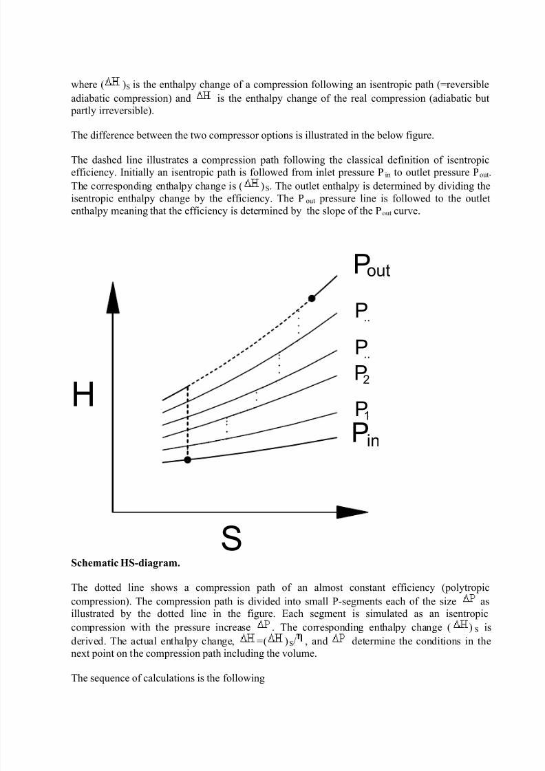
7/18/2019 PVTsim Tutorial Calsep
http://slidepdf.com/reader/full/pvtsim-tutorial-calsep 79/140
where ( )S is the enthalpy change of a compression following an isentropic path (=reversibleadiabatic compression) and is the enthalpy change of the real compression (adiabatic but
partly irreversible).
The difference between the two compressor options is illustrated in the below figure.
The dashed line illustrates a compression path following the classical definition of isentropicefficiency. Initially an isentropic path is followed from inlet pressure Pin to outlet pressure Pout.The corresponding enthalpy change is ( )S. The outlet enthalpy is determined by dividing theisentropic enthalpy change by the efficiency. The Pout pressure line is followed to the outletenthalpy meaning that the efficiency is determined by the slope of the Pout curve.
P
Pout
in
S
H
P
P
P
P1
2
..
..
Schematic HS-diagram.
The dotted line shows a compression path of an almost constant efficiency (polytropiccompression). The compression path is divided into small P-segments each of the size asillustrated by the dotted line in the figure. Each segment is simulated as an isentropiccompression with the pressure increase . The corresponding enthalpy change ( )S isderived. The actual enthalpy change, =( )S/ , and determine the conditions in thenext point on the compression path including the volume.
The sequence of calculations is the following
7/18/2019 PVTsim Tutorial Calsep
http://slidepdf.com/reader/full/pvtsim-tutorial-calsep 80/140
1. Divide the compression into n pressure steps where each step is =(Pout-Pin)/n.2. Perform a PT-flash for Tin, Pin. Flash determines Sin and Hin.3. Perform a PS-flash for P2=Pin + , Sin. Flash determines isentropic outlet temperature (T2)S
and (H2)S from segment.
4. Determine5. Determine T2 and S2 by PH-flash for P2,H2.6. Perform a PS-flash for P3=P2+ , S2. Flash determines isentropic temperature (T3)S and
(H3)S
7. Determine8. Determine T3 and S3 by PH flash for P3,H3.9. Continue from 6. with P4, and so on until Pn-1 (Pn=outlet pressure Pout).
The outlined procedure is applicable to gases as well as mixtures of gases and liquids.
The output for the Path of Constant Efficiency (PACE) option includes maximum and minimumvalues of the compressibility functions, X and Y as defined by Schultz (1962)
T
P
P
V
V
PY
1T
V
V
TX
∂∂
=
−
∂∂
=
Also given in the output is the HEAD defined as
f mg
WORK HEAD =
where WORK is the total work done by the compressor on the fluid, g the gravitationalacceleration and mf the flow rate of the fluid through the compresor.
As can be seen from the above equation, the unit of HEAD is m or ft depending on selected unit.HEAD therefore expreses the vertical lift height corresponding to the total work done by thecompressor on the fluid.
Expander
The input is inlet pressure and temperature and outlet pressure. An efficiency can be specifiedwhich is 1.0 by default. For an efficiency of 1 the expansion process is assumed to be isentropic(constant entropy (S)). In general the efficiency is defined as
7/18/2019 PVTsim Tutorial Calsep
http://slidepdf.com/reader/full/pvtsim-tutorial-calsep 81/140
( )s∆H
∆Hη=
where is the enthalpy change by an isentropic expansion and the actual enthalpy
change.
Cooler
Input consists of inlet and outlet temperature and pressure. The outlet pressure is entered as a pressure drop, which is zero by default. The cooling capacity is calculated which is the enthalpyto be removed from the flowing stream per time unit.
Heater
Input consists of inlet and outlet temperature and pressure. The outlet pressure is entered as a pressure drop, which is zero by default. The heating capacity is calculated which is the enthalpyto be transferred to the flowing stream per time unit.
Pump
Input consists of inlet temperature and pressure and outlet pressure. A thermal efficiency can bespecified, which is defined through the relation
∆H
P)V(Vη inout ∆+
=
where Vout is the outlet volume, Vin the inlet volume and the enthalpy change as a result ofthe pumping.
Valve
The outlet temperature is found by assuming that there is no enthalpy change by the passage ofthe valve.
Separator
Input consists of inlet temperature and pressure for which a PT-flash calculation is performed.
References
Schultz, J. M., "The Polytropic Analysis of Centrifugal Compressors", Journal of Engineering forPower, January 1962, pp. 69-82.
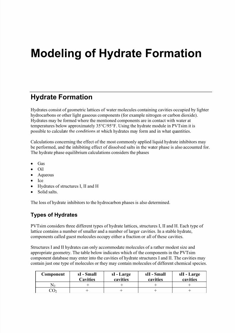
7/18/2019 PVTsim Tutorial Calsep
http://slidepdf.com/reader/full/pvtsim-tutorial-calsep 82/140
Modeling of Hydrate Formation
Hydrate Formation
Hydrates consist of geometric lattices of water molecules containing cavities occupied by lighter
hydrocarbons or other light gaseous components (for example nitrogen or carbon dioxide).Hydrates may be formed where the mentioned components are in contact with water attemperatures below approximately 35°C/95°F. Using the hydrate module in PVTsim it is
possible to calculate the conditions at which hydrates may form and in what quantities.
Calculations concerning the effect of the most commonly applied liquid hydrate inhibitors may be performed, and the inhibiting effect of dissolved salts in the water phase is also accounted for.The hydrate phase equilibrium calculations considers the phases
• Gas• Oil• Aqueous• Ice• Hydrates of structures I, II and H• Solid salts.
The loss of hydrate inhibitors to the hydrocarbon phases is also determined.
Types of Hydrates
PVTsim considers three different types of hydrate lattices, structures I, II and H. Each type oflattice contains a number of smaller and a number of larger cavities. In a stable hydrate,components called guest molecules occupy either a fraction or all of these cavities.
Structures I and II hydrates can only accommodate molecules of a rather modest size andappropriate geometry. The table below indicates which of the components in the PVTsimcomponent database may enter into the cavities of hydrate structures I and II. The cavities maycontain just one type of molecules or they may contain molecules of different chemical species.
Component sI - Small
Cavities
sI - Large
cavities
sII - Small
cavities
sII - Large
cavities
N2 + + + +CO2 + + + +
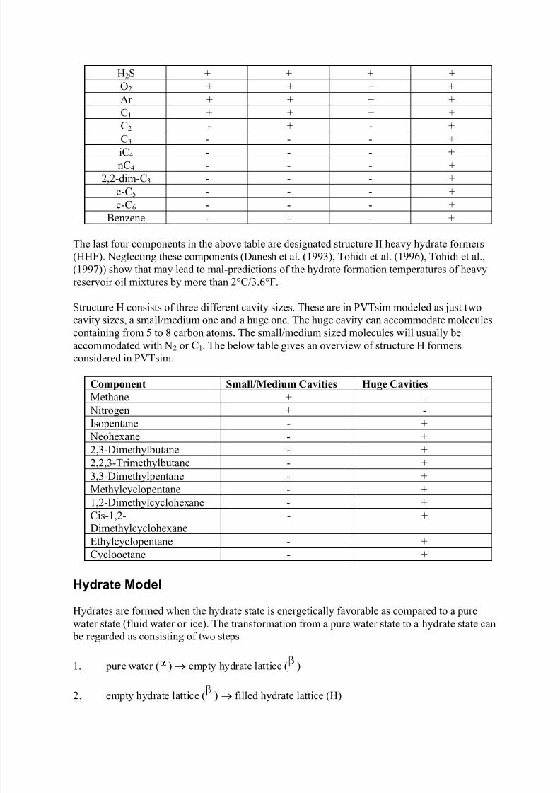
7/18/2019 PVTsim Tutorial Calsep
http://slidepdf.com/reader/full/pvtsim-tutorial-calsep 83/140
H2S + + + +O2 + + + +Ar + + + +C1 + + + +C2 - + - +
C3 - - - +iC4 - - - +nC4 - - - +
2,2-dim-C3 - - - +c-C5 - - - +c-C6 - - - +
Benzene - - - +
The last four components in the above table are designated structure II heavy hydrate formers(HHF). Neglecting these components (Danesh et al. (1993), Tohidi et al. (1996), Tohidi et al.,
(1997)) show that may lead to mal-predictions of the hydrate formation temperatures of heavyreservoir oil mixtures by more than 2°C/3.6°F.
Structure H consists of three different cavity sizes. These are in PVTsim modeled as just twocavity sizes, a small/medium one and a huge one. The huge cavity can accommodate moleculescontaining from 5 to 8 carbon atoms. The small/medium sized molecules will usually beaccommodated with N2 or C1. The below table gives an overview of structure H formersconsidered in PVTsim.
Component Small/Medium Cavities Huge Cavities
Methane + -
Nitrogen + -Isopentane - +
Neohexane - +2,3-Dimethylbutane - +2,2,3-Trimethylbutane - +3,3-Dimethylpentane - +Methylcyclopentane - +1,2-Dimethylcyclohexane - +Cis-1,2-Dimethylcyclohexane
- +
Ethylcyclopentane - +Cyclooctane - +
Hydrate Model
Hydrates are formed when the hydrate state is energetically favorable as compared to a purewater state (fluid water or ice). The transformation from a pure water state to a hydrate state can
be regarded as consisting of two steps
1. pure water ( ) → empty hydrate lattice ( )
2. empty hydrate lattice ( ) → filled hydrate lattice (H)
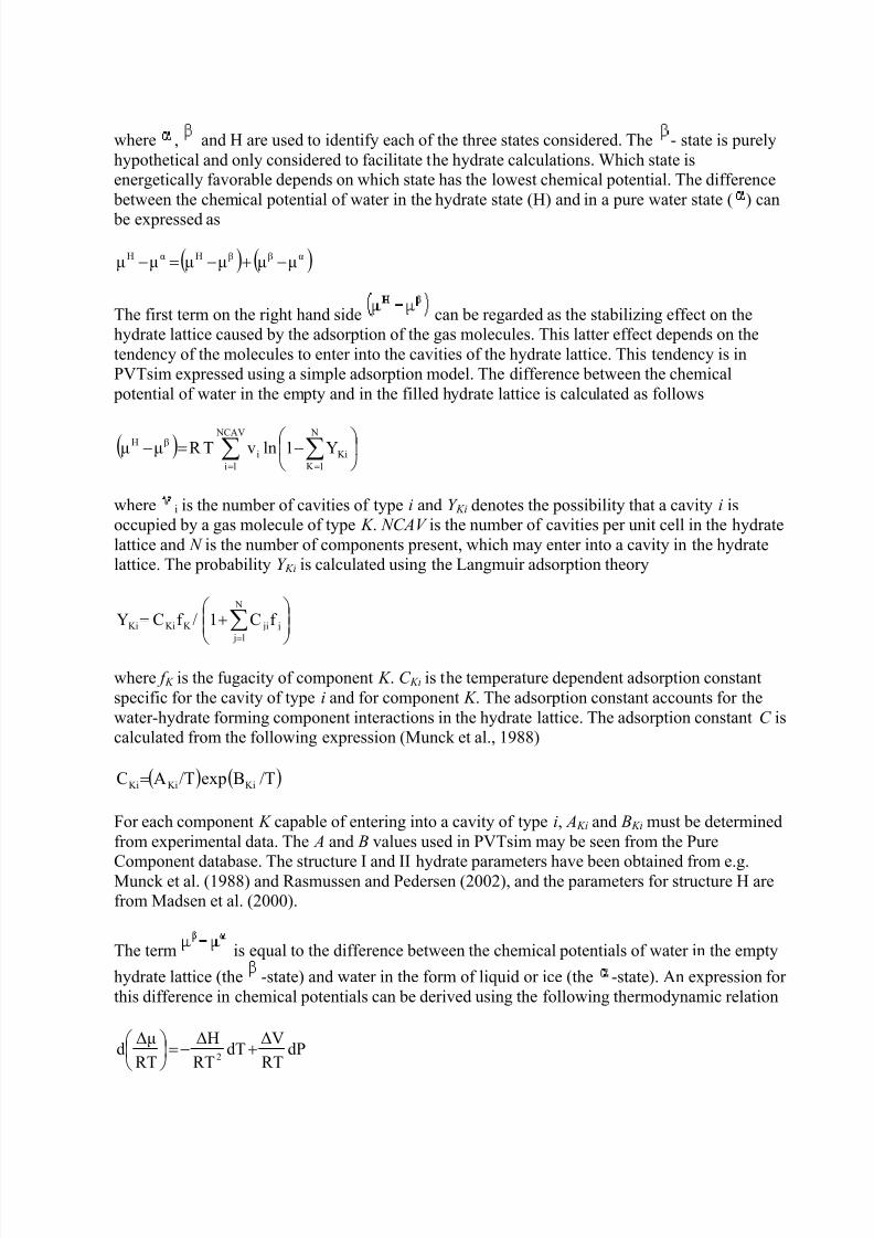
7/18/2019 PVTsim Tutorial Calsep
http://slidepdf.com/reader/full/pvtsim-tutorial-calsep 84/140
where , and H are used to identify each of the three states considered. The - state is purelyhypothetical and only considered to facilitate the hydrate calculations. Which state isenergetically favorable depends on which state has the lowest chemical potential. The difference
between the chemical potential of water in the hydrate state (H) and in a pure water state ( ) can
be expressed as
( ) ( )αββHαH µµµµµµ −+−=−
The first term on the right hand side can be regarded as the stabilizing effect on thehydrate lattice caused by the adsorption of the gas molecules. This latter effect depends on thetendency of the molecules to enter into the cavities of the hydrate lattice. This tendency is inPVTsim expressed using a simple adsorption model. The difference between the chemical
potential of water in the empty and in the filled hydrate lattice is calculated as follows
( ) ∑ ∑= =
−=−
NCAV
li
N
1K Kii
βH Y1lnvTR µµ
where i is the number of cavities of type i and Y Ki denotes the possibility that a cavity i isoccupied by a gas molecule of type K . NCAV is the number of cavities per unit cell in the hydratelattice and N is the number of components present, which may enter into a cavity in the hydratelattice. The probability Y Ki is calculated using the Langmuir adsorption theory
+= ∑
=
N
l j
j jiK KiKi f C1/f CY
where f K is the fugacity of component K . C Ki is the temperature dependent adsorption constantspecific for the cavity of type i and for component K . The adsorption constant accounts for thewater-hydrate forming component interactions in the hydrate lattice. The adsorption constant C iscalculated from the following expression (Munck et al., 1988)
( ) ( /TBexp/TAC KiKiKi= )
For each component K capable of entering into a cavity of type i, A Ki and B Ki must be determinedfrom experimental data. The A and B values used in PVTsim may be seen from the PureComponent database. The structure I and II hydrate parameters have been obtained from e.g.Munck et al. (1988) and Rasmussen and Pedersen (2002), and the parameters for structure H arefrom Madsen et al. (2000).
The term is equal to the difference between the chemical potentials of water in the empty
hydrate lattice (the -state) and water in the form of liquid or ice (the -state). An expression forthis difference in chemical potentials can be derived using the following thermodynamic relation
dP
RT
∆VdT
RT
∆H
RT
∆µd
2 +−=
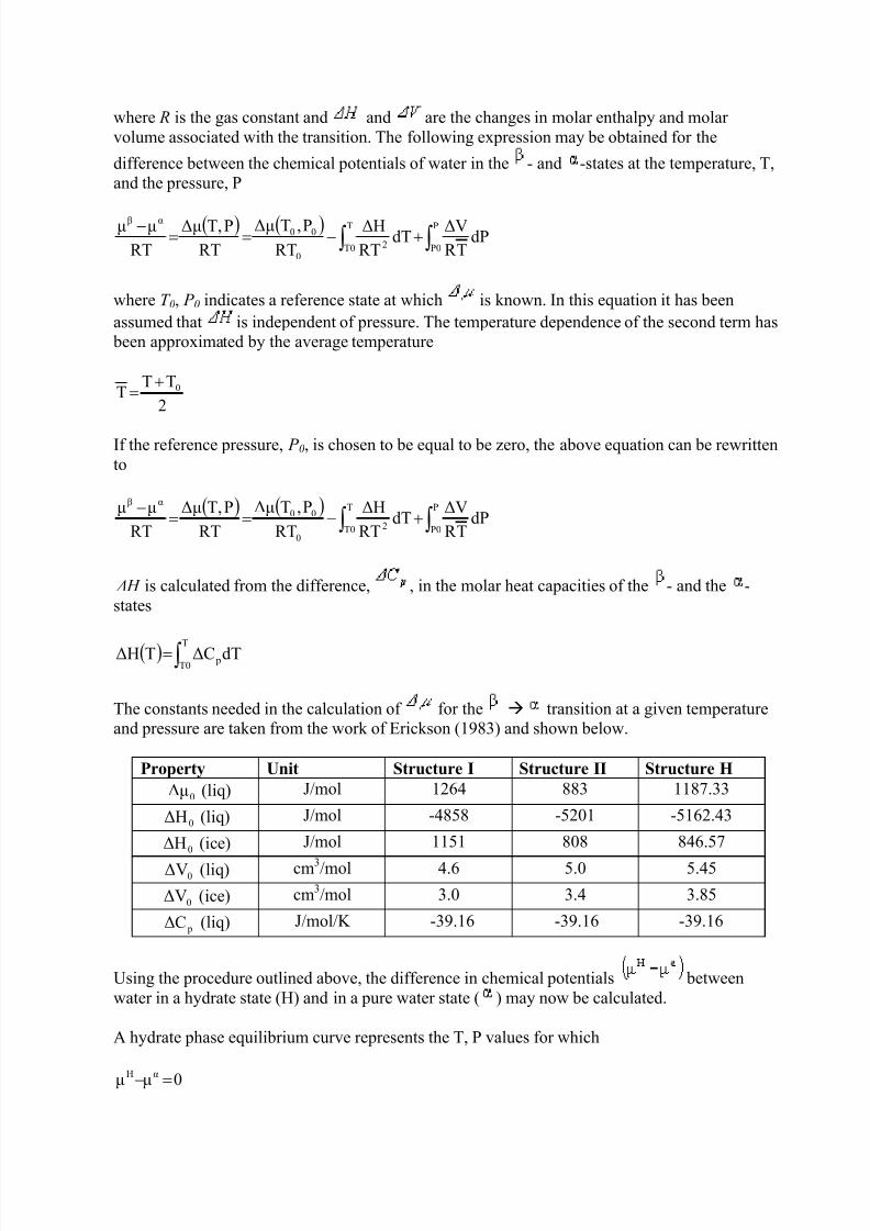
7/18/2019 PVTsim Tutorial Calsep
http://slidepdf.com/reader/full/pvtsim-tutorial-calsep 85/140
where R is the gas constant and and are the changes in molar enthalpy and molarvolume associated with the transition. The following expression may be obtained for the
difference between the chemical potentials of water in the - and -states at the temperature, T,and the pressure, P
( ) ( )∫∫ +−==
− P
P0
T
T0 20
00αβ
dPTR
∆VdT
RT
∆H
RT
P,T∆µ
RT
PT,∆µ
RT
µµ
where T 0, P 0 indicates a reference state at which is known. In this equation it has beenassumed that is independent of pressure. The temperature dependence of the second term has
been approximated by the average temperature
2
TTT 0+
=
If the reference pressure, P 0, is chosen to be equal to be zero, the above equation can be rewrittento
( ) ( )∫∫ +−==
− P
P0
T
T0 20
00αβ
dPTR
∆VdT
RT
∆H
RT
P,T∆µ
RT
PT,∆µ
RT
µµ
∆ H is calculated from the difference, , in the molar heat capacities of the - and the -states
( ) ∫=T
T0 pdT∆CT∆H
The constants needed in the calculation of for the transition at a given temperatureand pressure are taken from the work of Erickson (1983) and shown below.
Property Unit Structure I Structure II Structure H
0∆µ (liq) J/mol 1264 883 1187.33
0∆H (liq) J/mol -4858 -5201 -5162.43
0∆H (ice) J/mol 1151 808 846.570∆V (liq) cm3/mol 4.6 5.0 5.45
0∆V (ice) cm3/mol 3.0 3.4 3.85
p∆C (liq) J/mol/K -39.16 -39.16 -39.16
Using the procedure outlined above, the difference in chemical potentials betweenwater in a hydrate state (H) and in a pure water state ( ) may now be calculated.
A hydrate phase equilibrium curve represents the T, P values for which
0µµ αH =−
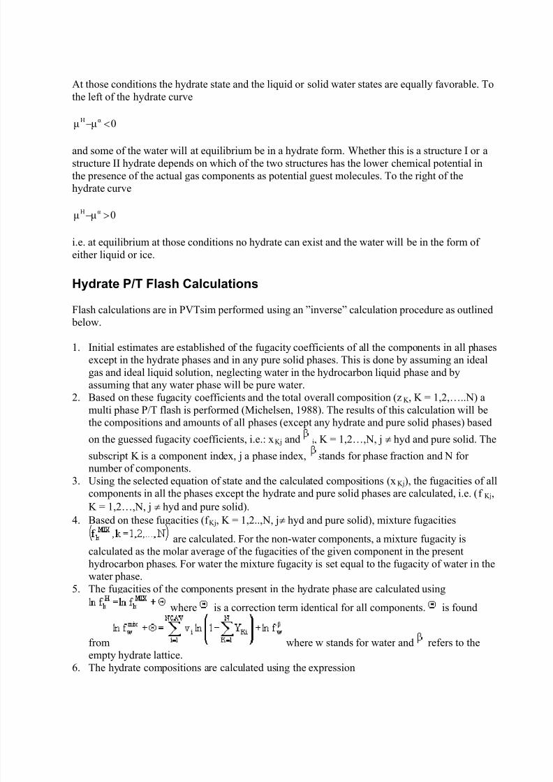
7/18/2019 PVTsim Tutorial Calsep
http://slidepdf.com/reader/full/pvtsim-tutorial-calsep 86/140
At those conditions the hydrate state and the liquid or solid water states are equally favorable. Tothe left of the hydrate curve
0µµ αH <−
and some of the water will at equilibrium be in a hydrate form. Whether this is a structure I or astructure II hydrate depends on which of the two structures has the lower chemical potential inthe presence of the actual gas components as potential guest molecules. To the right of thehydrate curve
0µµ αH >−
i.e. at equilibrium at those conditions no hydrate can exist and the water will be in the form ofeither liquid or ice.
Hydrate P/T Flash Calculations
Flash calculations are in PVTsim performed using an ”inverse” calculation procedure as outlined below.
1. Initial estimates are established of the fugacity coefficients of all the components in all phasesexcept in the hydrate phases and in any pure solid phases. This is done by assuming an idealgas and ideal liquid solution, neglecting water in the hydrocarbon liquid phase and byassuming that any water phase will be pure water.
2. Based on these fugacity coefficients and the total overall composition (zK , K = 1,2,…..N) amulti phase P/T flash is performed (Michelsen, 1988). The results of this calculation will bethe compositions and amounts of all phases (except any hydrate and pure solid phases) based
on the guessed fugacity coefficients, i.e.: xKj and j, K = 1,2…,N, j ≠ hyd and pure solid. The
subscript K is a component index, j a phase index, stands for phase fraction and N fornumber of components.
3. Using the selected equation of state and the calculated compositions (xKj), the fugacities of allcomponents in all the phases except the hydrate and pure solid phases are calculated, i.e. (f Kj,K = 1,2…,N, j ≠ hyd and pure solid).
4. Based on these fugacities (f Kj, K = 1,2..,N, j≠ hyd and pure solid), mixture fugacities
are calculated. For the non-water components, a mixture fugacity iscalculated as the molar average of the fugacities of the given component in the presenthydrocarbon phases. For water the mixture fugacity is set equal to the fugacity of water in thewater phase.
5. The fugacities of the components present in the hydrate phase are calculated using
where is a correction term identical for all components. is found
from where w stands for water and refers to theempty hydrate lattice.
6. The hydrate compositions are calculated using the expression
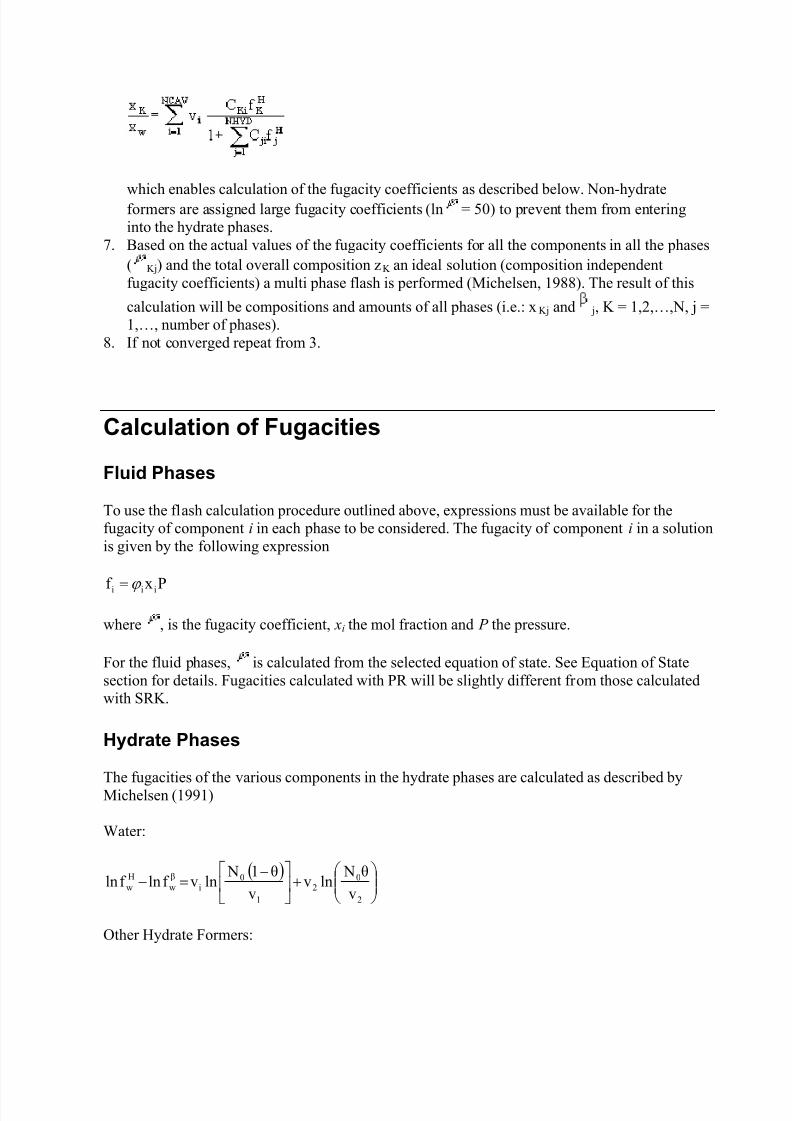
7/18/2019 PVTsim Tutorial Calsep
http://slidepdf.com/reader/full/pvtsim-tutorial-calsep 87/140
which enables calculation of the fugacity coefficients as described below. Non-hydrateformers are assigned large fugacity coefficients (ln = 50) to prevent them from enteringinto the hydrate phases.
7. Based on the actual values of the fugacity coefficients for all the components in all the phases( Kj) and the total overall composition zK an ideal solution (composition independentfugacity coefficients) a multi phase flash is performed (Michelsen, 1988). The result of this
calculation will be compositions and amounts of all phases (i.e.: xKj and j, K = 1,2,…,N, j =1,…, number of phases).
8. If not converged repeat from 3.
Calculation of Fugacities
Fluid Phases
To use the flash calculation procedure outlined above, expressions must be available for thefugacity of component i in each phase to be considered. The fugacity of component i in a solutionis given by the following expression
Pxf iii ϕ =
where , is the fugacity coefficient, xi the mol fraction and P the pressure.
For the fluid phases, is calculated from the selected equation of state. See Equation of Statesection for details. Fugacities calculated with PR will be slightly different from those calculatedwith SRK.
Hydrate Phases
The fugacities of the various components in the hydrate phases are calculated as described byMichelsen (1991)
Water:
( )
+
−=−
2
02
1
0i
β
wHw v
θ Nlnv
v
θ1 Nlnvf lnf ln
Other Hydrate Formers:
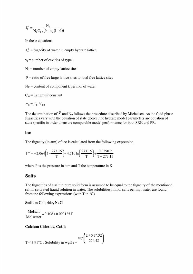
7/18/2019 PVTsim Tutorial Calsep
http://slidepdf.com/reader/full/pvtsim-tutorial-calsep 88/140
( )( )θ1αθC N
Nf
k 2k 0
k Hk −+
=
In these equations
β
wf = fugacity of water in empty hydrate lattice
vi = number of cavities of type i
N0 = number of empty lattice sites
θ = ratio of free large lattice sites to total free lattice sites
NK = content of component k per mol of water
Cki = Langmuir constant
α k = Ck1/Ck2
The determination of and N0 follows the procedure described by Michelsen. As the fluid phasefugacities vary with the equation of state choice, the hydrate model parameters are equation ofstate specific in order to ensure comparable model performance for both SRK and PR.
Ice
The fugacity (in atm) of ice is calculated from the following expression
273.15T
P0.0390
T
273.15ln4.710
T
273.1512.064f ice
++
−
−−=
where P is the pressure in atm and T the temperature in K.
Salts
The fugacities of a salt in pure solid form is assumed to be equal to the fugacity of the mentioned
salt in saturated liquid solution in water. The solubilities in mol salts per mol water are foundfrom the following expressions (with T in °C)
Sodium Chloride, NaCl
T0.0001250.108water Mol
saltMol+=
Calcium Chloride, CaCl2
T < 3.91°C : Solubility in wgt% =
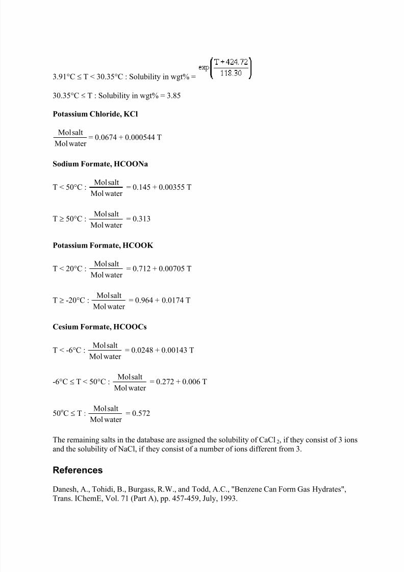
7/18/2019 PVTsim Tutorial Calsep
http://slidepdf.com/reader/full/pvtsim-tutorial-calsep 89/140
3.91°C ≤ T < 30.35°C : Solubility in wgt% =
30.35°C ≤ T : Solubility in wgt% = 3.85
Potassium Chloride, KCl
water Mol
saltMol= 0.0674 + 0.000544 T
Sodium Formate, HCOONa
T < 50°C :
water Mol
saltMol = 0.145 + 0.00355 T
T ≥ 50°C :water Mol
saltMol = 0.313
Potassium Formate, HCOOK
T < 20°C :water Mol
saltMol = 0.712 + 0.00705 T
T ≥ -20°C :water MolsaltMol = 0.964 + 0.0174 T
Cesium Formate, HCOOCs
T < -6°C :water Mol
saltMol = 0.0248 + 0.00143 T
-6°C ≤ T < 50°C :water Mol
saltMol = 0.272 + 0.006 T
50oC ≤ T :water Mol
saltMol = 0.572
The remaining salts in the database are assigned the solubility of CaCl2, if they consist of 3 ionsand the solubility of NaCl, if they consist of a number of ions different from 3.
References
Danesh, A., Tohidi, B., Burgass, R.W., and Todd, A.C., "Benzene Can Form Gas Hydrates",Trans. IChemE, Vol. 71 (Part A), pp. 457-459, July, 1993.
7/18/2019 PVTsim Tutorial Calsep
http://slidepdf.com/reader/full/pvtsim-tutorial-calsep 90/140
Erickson, D.D., ”Development of a Natural Gas Hydrate Prediction Computer Program”, M. Sc.thesis, Colorado School of Mines, 1983.
Madsen, J., Pedersen, K.S. and Michelsen, M.L., ”Modeling of Structure H Hydrates using a
Langmuir Adsorption Model”, Ind. Eng. Chem. Res., 39, 2000, pp. 1111-1114.
Michelsen, M.L., ”Calculation of Multiphase Equilibrium in Ideal Solutions”, SEP 8802, TheDepartment of Chemical Engineering, The Technical University of Denmark, 1988.
Michelsen, M.L., ”Calculation of Hydrate fugacities ”, Chem. Eng. Sci. 46, 1991, 1192-1193.
Munck, J., Skjold-Jørgensen S. and Rasmussen, P., ”Computations of the Formation of GasHydrates”, Chem. Eng. Sci. 43, 1988, 2661-2672.
Rasmussen, C.P. and Pedersen, K.S., “Challenges in Modeling of Gas Hydrate Phase Equilibria”,
4th International Conference on Gas Hydrates Yokohama Japan, May 19 - 23, 2002.
Tohidi, B., Danesh, A., Burgass, R.W., and Todd, A.C., “Equilibrium Data and ThermodynamicModelling of Cyclohexane Gas Hydrates”, Chem. Eng. Sci., Vol. 51, No. 1, pp. 159-163, 1996.
Tohidi, B., Danesh, A., Todd, A.C., Burgass, R.W., Østergaard, K.K., "Equilibrium Data andThermodynamic Modelling of Cyclopentane and Neopentane Hydrates", Fluid Phase Equilibria138, pp. 241-250, 1997.
7/18/2019 PVTsim Tutorial Calsep
http://slidepdf.com/reader/full/pvtsim-tutorial-calsep 91/140
Modeling of Wax Formation
Modeling of Wax Formation
The wax module of PVTsim may be used to determine the wax appearance temperature (cloud point) at a given pressure, the wax appearance pressure at a given temperature and to perform PTflash calculations taking into consideration the possible formation of a wax phase in addition togas and oil phases. The wax model used is that of Pedersen (1995) extended as proposed byRønningsen et al. (1997).
Vapor-Liquid-Wax Phase Equilibria
At thermodynamic equilibrium between a liquid (oil) and a solid (wax) phase, the fugacity, ,
of component i in the liquid phase equals the fugacity, , of component i in the solid phase
Si
Li f f =
When a cubic equation of state is used for the liquid phase it is practical to express the liquid phase fugacities in terms of fugacity coefficients
Pxf Li
Li
Li ϕ =
In this expression is the liquid phase mol fraction of component i, the liquid phasefugacity coefficient of component i and P the pressure. For an ideal solid phase mixture, the solid phase fugacity of component i can be expressed as
oSi
Si
Si f xf =
where is the solid phase mol fraction of component i, andSix the solid standard state fugacity
of component i. The solid standard state fugacity is related to the liquid standard state fugacity as
( )( )
= ref oLi
ref oSif
i Pf
Pf
lnRT∆G

7/18/2019 PVTsim Tutorial Calsep
http://slidepdf.com/reader/full/pvtsim-tutorial-calsep 92/140
where is the molar change in Gibbs free energy associated with the transition of pure
component i from solid to liquid form at the temperature of the system. To calculate thefollowing general thermodynamic relation is used
ST∆H∆G ∆−=
where stands for change in enthalpy and for change in entropy. Neglecting any
differences between the liquid and solid phase heat capacities, may be expressed as
f i
f i
f i ST∆H∆G ∆+=
where is the enthalpy and the entropy of fusion of component i at the normal melting
point. Again neglecting any differences between the liquid and solid state heat capacities, theentropy of fusion may be expressed as follows in terms of the enthalpy of fusion
f i
f if
iT
∆H∆S =
where is the melting temperature of component i. The following expression may now bederived for the solid standard state fugacity of component i
( ) ( )
−+
−
−= RT
PP∆V
T
T1RT
∆HexpPf f ref if
i
f
iref oLioSi
where is the difference between the solid and liquid phase molar volumes. Based on
experimental observations of Templin (1956), the difference i between the solid and liquid phase molar volumes of component i is assumed to be 10% of the liquid molar volume, i.e. thesolidification process is assumed to be associated with a 10% volume decrease.
The liquid standard state fugacity of component i may be expressed as follows
Pf oLi
oLi ϕ =
where is the liquid phase fugacity coefficient of pure i at the system temperature and pressure. This leads to
( ) ( )
−+
−
−=
RT
PP∆V
T
T1
RT
∆HexpPPf ref i
f i
f i
ref oLi
oSi ϕ
The following expression may now be derived for the solid phase fugacity of component i in a
mixture
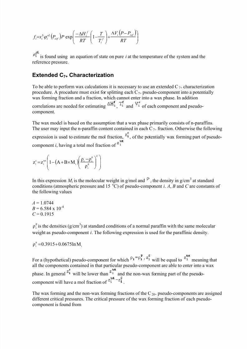
7/18/2019 PVTsim Tutorial Calsep
http://slidepdf.com/reader/full/pvtsim-tutorial-calsep 93/140
( ) ( )
−∆+
−
∆−=
RT
P P V
T
T
RT
H P P x f
ref i
f
i
f
iref
oL
i
S
ii 1expϕ
is found using an equation of state on pure i at the temperature of the system and thereference pressure.
Extended C7+ Characterization
To be able to perform wax calculations it is necessary to use an extended C7+ characterization procedure. A procedure must exist for splitting each C7+ pseudo-component into a potentiallywax forming fraction and a fraction, which cannot enter into a wax phase. In addition
correlations are needed for estimating , and of each component and pseudo-component.
The wax model is based on the assumption that a wax phase primarily consists of n-paraffins.The user may input the n-paraffin content contained in each C7+ fraction. Otherwise the following
expression is used to estimate the mol fraction, , of the potentially wax forming part of pseudo-
component i, having a total mol fraction of
( )
−×+−=
C
P
i
P
iii
tot
i
s
iρ
ρρMBA1zz
In this expression M i is the molecular weight in g/mol and i the density in g/cm3 at standardconditions (atmospheric pressure and 15 oC) of pseudo-component i. A, B and C are constants ofthe following values
A = 1.0744 B = 6.584 x 10⁻⁴ C = 0.1915
Piρ is the densities (g/cm3) at standard conditions of a normal paraffin with the same molecular
weight as pseudo-component i. The following expression is used for the paraffinic density.
i
P
i Mln0.06750.3915ρ +=
For a (hypothetical) pseudo-component for which will be equal to meaning thatall the components contained in that particular pseudo-component are able to enter into a wax
phase. In general will be lower than and the non-wax forming part of the pseudo-
component will have a mol fraction of .
The wax forming and the non-wax forming fractions of the C20+ pseudo-components are assigned
different critical pressures. The critical pressure of the wax forming fraction of each pseudo-component is found from
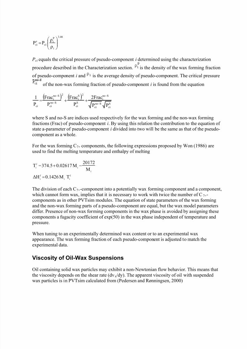
7/18/2019 PVTsim Tutorial Calsep
http://slidepdf.com/reader/full/pvtsim-tutorial-calsep 94/140
3.46
i
Pi
cisci
ρ
ρPP
=
P ci equals the critical pressure of pseudo-component i determined using the characterization procedure described in the Characterization section. is the density of the wax forming fraction
of pseudo-component i and is the average density of pseudo-component. The critical pressure
of the non-wax forming fraction of pseudo-component i is found from the equation
( ) ( )Sci
Snoci
Snoi
Sci
2Si
2
Snoci
Snoi
ci PP
2Frac
P
Frac
P
Frac
P
1−
−
−
−
++=
where S and no-S are indices used respectively for the wax forming and the non-wax formingfractions (Frac) of pseudo-component i. By using this relation the contribution to the equation ofstate a-parameter of pseudo-component i divided into two will be the same as that of the pseudo-component as a whole.
For the wax forming C7+ components, the following expressions proposed by Won (1986) areused to find the melting temperature and enthalpy of melting
f
ii
f
i
i
i
f
i
TM0.1426∆H
M
20172M0.02617374.5T
=
−+=
The division of each C7+-component into a potentially wax forming component and a component,which cannot form wax, implies that it is necessary to work with twice the number of C7+-components as in other PVTsim modules. The equation of state parameters of the wax formingand the non-wax forming parts of a pseudo-component are equal, but the wax model parametersdiffer. Presence of non-wax forming components in the wax phase is avoided by assigning thesecomponents a fugacity coefficient of exp(50) in the wax phase independent of temperature and
pressure.
When tuning to an experimentally determined wax content or to an experimental wax
appearance. The wax forming fraction of each pseudo-component is adjusted to match theexperimental data.
Viscosity of Oil-Wax Suspensions
Oil containing solid wax particles may exhibit a non-Newtonian flow behavior. This means thatthe viscosity depends on the shear rate (dvx/dy). The apparent viscosity of oil with suspendedwax particles is in PVTsim calculated from (Pedersen and Rønningsen, 2000)
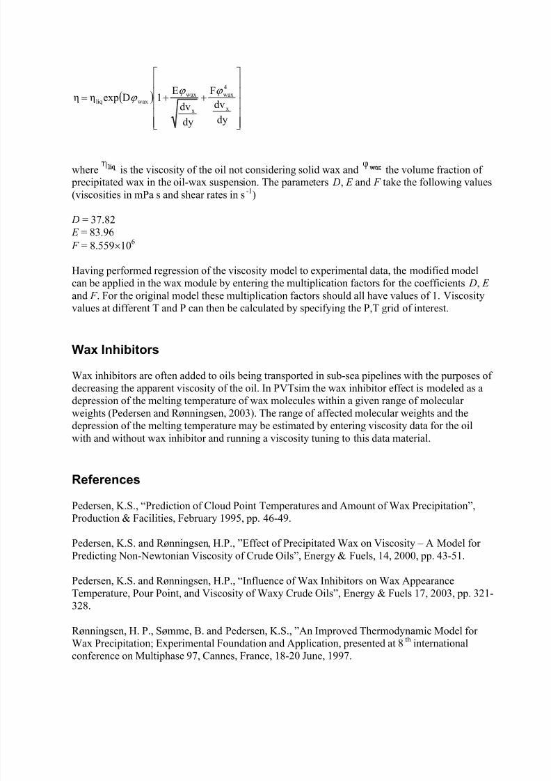
7/18/2019 PVTsim Tutorial Calsep
http://slidepdf.com/reader/full/pvtsim-tutorial-calsep 95/140
( )
++=
dy
dvF
dy
dv
E1Dexpηη
x
4wax
x
waxwaxliq
ϕ ϕ ϕ
where is the viscosity of the oil not considering solid wax and the volume fraction of precipitated wax in the oil-wax suspension. The parameters D, E and F take the following values(viscosities in mPa s and shear rates in s-1)
D = 37.82 E = 83.96 F = 8.559×10⁶
Having performed regression of the viscosity model to experimental data, the modified modelcan be applied in the wax module by entering the multiplication factors for the coefficients D, E and F . For the original model these multiplication factors should all have values of 1. Viscosityvalues at different T and P can then be calculated by specifying the P,T grid of interest.
Wax Inhibitors
Wax inhibitors are often added to oils being transported in sub-sea pipelines with the purposes ofdecreasing the apparent viscosity of the oil. In PVTsim the wax inhibitor effect is modeled as a
depression of the melting temperature of wax molecules within a given range of molecularweights (Pedersen and Rønningsen, 2003). The range of affected molecular weights and thedepression of the melting temperature may be estimated by entering viscosity data for the oilwith and without wax inhibitor and running a viscosity tuning to this data material.
References
Pedersen, K.S., “Prediction of Cloud Point Temperatures and Amount of Wax Precipitation”,Production & Facilities, February 1995, pp. 46-49.
Pedersen, K.S. and Rønningsen, H.P., ”Effect of Precipitated Wax on Viscosity – A Model forPredicting Non-Newtonian Viscosity of Crude Oils”, Energy & Fuels, 14, 2000, pp. 43-51.
Pedersen, K.S. and Rønningsen, H.P., “Influence of Wax Inhibitors on Wax AppearanceTemperature, Pour Point, and Viscosity of Waxy Crude Oils”, Energy & Fuels 17, 2003, pp. 321-328.
Rønningsen, H. P., Sømme, B. and Pedersen, K.S., ”An Improved Thermodynamic Model forWax Precipitation; Experimental Foundation and Application, presented at 8th internationalconference on Multiphase 97, Cannes, France, 18-20 June, 1997.
7/18/2019 PVTsim Tutorial Calsep
http://slidepdf.com/reader/full/pvtsim-tutorial-calsep 96/140
Templin, R.D., “Coefficient of Volume Expansion for Petroleum Waxes and Pure n-Paraffins”,Ind. Eng. Chem., 48, 1956, pp. 154-161.
Won, K.W., ”Thermodynamics for Solid-Liquid-Vapor Equilibria: Wax Phase Formation fromHeavy Hydrocarbon Mixtures”, Fluid Phase Equilibria 30, 1986, pp. 265-279.
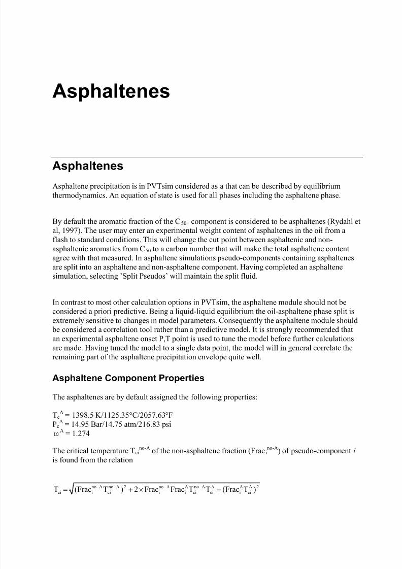
7/18/2019 PVTsim Tutorial Calsep
http://slidepdf.com/reader/full/pvtsim-tutorial-calsep 97/140
Asphaltenes
Asphaltenes
Asphaltene precipitation is in PVTsim considered as a that can be described by equilibrium
thermodynamics. An equation of state is used for all phases including the asphaltene phase.
By default the aromatic fraction of the C50+ component is considered to be asphaltenes (Rydahl etal, 1997). The user may enter an experimental weight content of asphaltenes in the oil from aflash to standard conditions. This will change the cut point between asphaltenic and non-asphaltenic aromatics from C50 to a carbon number that will make the total asphaltene contentagree with that measured. In asphaltene simulations pseudo-components containing asphaltenesare split into an asphaltene and non-asphaltene component. Having completed an asphaltenesimulation, selecting ’Split Pseudos’ will maintain the split fluid.
In contrast to most other calculation options in PVTsim, the asphaltene module should not beconsidered a priori predictive. Being a liquid-liquid equilibrium the oil-asphaltene phase split isextremely sensitive to changes in model parameters. Consequently the asphaltene module should
be considered a correlation tool rather than a predictive model. It is strongly recommended thatan experimental asphaltene onset P,T point is used to tune the model before further calculationsare made. Having tuned the model to a single data point, the model will in general correlate theremaining part of the asphaltene precipitation envelope quite well.
Asphaltene Component Properties
The asphaltenes are by default assigned the following properties:
TcA = 1398.5 K/1125.35°C/2057.63°F
PcA = 14.95 Bar/14.75 atm/216.83 psi
ωA = 1.274
The critical temperature Tcino-A of the non-asphaltene fraction (Fraci
no-A) of pseudo-component i is found from the relation
2Aci
Ai
Aci
Anoci
Ai
Anoi
2Anoci
Anoici )T(FracTTFracFrac2)T(FracT +×+=
−−−−
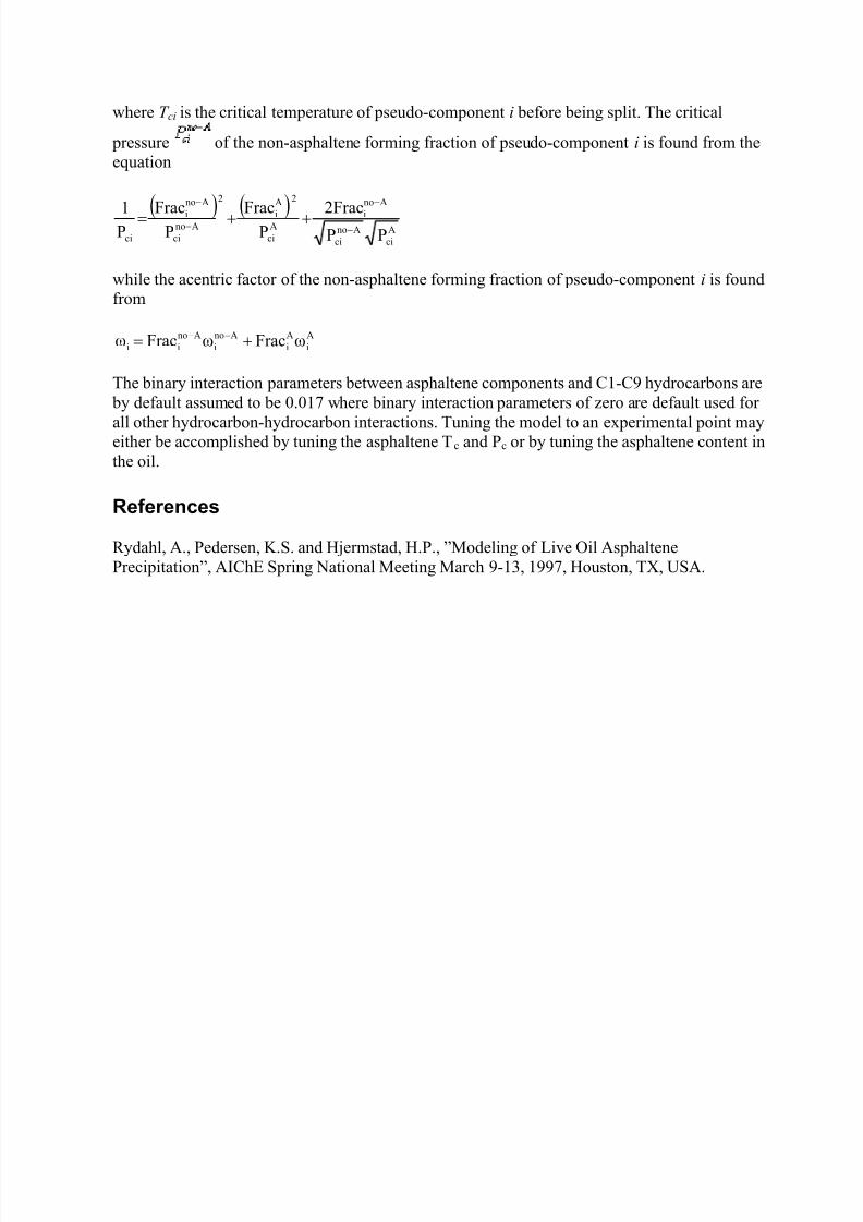
7/18/2019 PVTsim Tutorial Calsep
http://slidepdf.com/reader/full/pvtsim-tutorial-calsep 98/140
where T ci is the critical temperature of pseudo-component i before being split. The critical
pressure of the non-asphaltene forming fraction of pseudo-component i is found from theequation
( ) ( ) Aci
Anoci
Ano
iAci
2A
i
2
Anoci
Ano
i
ci PP2Frac
PFrac
PFrac
P1
−
−
−
−
++=
while the acentric factor of the non-asphaltene forming fraction of pseudo-component i is foundfrom
Ai
Ai
Anoi
Anoii ωFracωFracω += −−
The binary interaction parameters between asphaltene components and C1-C9 hydrocarbons are by default assumed to be 0.017 where binary interaction parameters of zero are default used for
all other hydrocarbon-hydrocarbon interactions. Tuning the model to an experimental point mayeither be accomplished by tuning the asphaltene Tc and Pc or by tuning the asphaltene content inthe oil.
References
Rydahl, A., Pedersen, K.S. and Hjermstad, H.P., ”Modeling of Live Oil AsphaltenePrecipitation”, AIChE Spring National Meeting March 9-13, 1997, Houston, TX, USA.
7/18/2019 PVTsim Tutorial Calsep
http://slidepdf.com/reader/full/pvtsim-tutorial-calsep 99/140
H2S Simulations
H2S Simulations
The H2S module of PVTsim is based on the same PT-flash as is used in many of the other
modules. What makes this module different is the way H2S is treated in the aqueous phase. Thedissociation of H2S is considered.
H2S ↔ HS- + H+
The degree of dissociation is determined by the pH
+−= Hlog pH 10
and pK
[ ][ ]SH
HHSlog pK
2
101
+−
=
pK 1 is calculated using considerations based on chemical reaction equilibria. This givesapproximately the following temperature dependence
pK 1 = 7.2617 – 0.01086(T – 273.15)
where T is the temperature in K. From the knowledge of the amount of dissolved H2S onmolecular form, pH and pK 1 it is straightforward to calculate [HS-].
In principle the following equilibrium should also be considered
HS- ↔ S-- + H+
Its pK value defined by the following expression
[ ][ ][ ]−
−−+
−=HS
SHlog pK 102
is however of the order 13-14, meaning that the second order dissociation for all practical purposes can be neglected. It is therefore not considered in the H2S module.
7/18/2019 PVTsim Tutorial Calsep
http://slidepdf.com/reader/full/pvtsim-tutorial-calsep 100/140
Water Phase Properties
Water Phase Properties
As a rough guideline PVTsim performs full 3 phase flash calculations on mixtures containing
aqueous components. However, the following interface modules treats a possible water phase as pure water, possibly containing salt. This applies for the interface modules to
- Dynalog- Prosper/Mbal- Multiphase meter interface if license does not give access to multiflash options.
The options treating water as pure water calculates the physical properties and transport properties using a separate thermodynamics instead of an EOS. In the OLGA2000 interface thewater property routines are used in cases where no hydrate inhibitors are present. This is also anoption in the Property Generator.
Properties of Pure Water
Thermodynamic Properties
The thermodynamic properties of pure water are calculated using an equation for Helmholtz freeenergy developed by Keyes et al. (1968)
( ) ( )[ ]T Q RT T ,ln0 ρ ρ ρ ++Ψ=Ψ
where
Ψ = Helmholtz free energy (J/g) ρ = Density (g/cm3)
τ = 1000/T where T is the temperature in KR = 0.46151 J/(g K)
and
( ) ( ) T T C C T C T C C T ln542
3210 ++++=Ψ
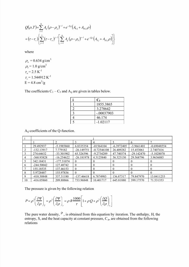
7/18/2019 PVTsim Tutorial Calsep
http://slidepdf.com/reader/full/pvtsim-tutorial-calsep 101/140
( ) ( ) ( )
( ) ( ) ( ) ( )
++−−−+
++−=
∑ ∑
∑
= =
−−−
=
−−
7
2
8
1109
2
8
1,101,9,
j i
j j
Epl o
bij
j
ac
l i
E l i
aij
A Ae A
A Ae AT Q
ρ ρ ρ τ τ τ τ
ρ ρ ρ ρ ρ
where
a ρ = 0.634 g/cm3
b ρ = 1.0 g/cm3
aτ = 2.5 K -1
cτ = 1.544912 K -1
E = 4.8 cm3/g
The coefficients C1 – C5 and Aij are given in tables below.
i CI
1 1855.38652 3.2786423 -.000379034 46.1745 -1.02117
Aij-coefficients of the Q-function.
i j1 2 3 4 5 6 7
1 29.492937 -5.1985860 6.8335354 -01564104 -6.3972405 -3.9661401 -0.690485542 -132.13917 7.779182 -26.149751 -0.72546108 26.409282 15.453061 2.74074163 274.64632 -33.301902 65.326396 -9.2734289 47.740374 -29.142470 -5.10280704 -360.93828 -16.254622 -26.181978 4.3125840 56.323130 29.568796 3.96360855 342.18431 -177.31074 0 0 0 0 06 -244.50042 127.48742 0 0 0 0 07 155.18535 137.46153 0 0 0 0 08 5.9728487 155.97836 0 0 0 0 09 -410.30848 337.31180 -137.46618 6.7874983 136.87317 79.847970 13.041125310 -416.05860 209.88866 733.96848 10.401717 645.81880 399.17570 71.531353
The pressure is given by the following relation
∂
∂++=
∂
Ψ∂=
∂
Ψ∂=
τ τ ρ
ρ ρ τ
ρ ρ
ρ ρ
ρ Q
Q R P T
222 11000
The pure water density, , is obtained from this equation by iteration. The enthalpy, H, theentropy, S, and the heat capacity at constant pressure, C p, are obtained from the followingrelations
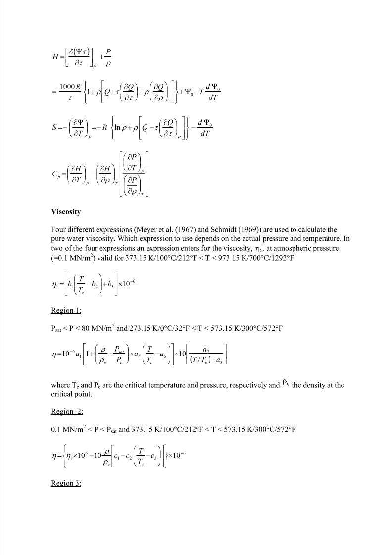
7/18/2019 PVTsim Tutorial Calsep
http://slidepdf.com/reader/full/pvtsim-tutorial-calsep 102/140
( ) ρ τ
τ
ρ
P H +
∂Ψ∂
=
dT
d T
QQQ
R 0
01
1000 Ψ−Ψ+
∂
∂+
∂
∂++=
τ ρ ρ
τ τ ρ
τ
dT
d QQ R
T S 0ln
Ψ−
∂∂
−+−=
∂Ψ∂
−= ρ ρ τ
τ ρ ρ
∂
∂
∂∂
∂∂
−
∂∂
=
T
T
p P
T
P
H
T
H C
ρ
ρ
ρ
ρ
Viscosity
Four different expressions (Meyer et al. (1967) and Schmidt (1969)) are used to calculate the pure water viscosity. Which expression to use depends on the actual pressure and temperature. Intwo of the four expressions an expression enters for the viscosity, , at atmospheric pressure
(=0.1 MN/m2) valid for 373.15 K/100°C/212°F < T < 973.15 K/700°C/1292°F
6
3211 10
−
×
+
−= bbT
T
b cη
Region 1:
Psat < P < 80 MN/m2 and 273.15 K/0°C/32°F < T < 573.15 K/300°C/572°F
( )
−×
−×
−+= −
3
2541
6
/10110
aT T
aa
T
T a
P
P a
ccc
sat
c ρ
ρ η
where Tc and Pc are the critical temperature and pressure, respectively and the density at thecritical point.
Region 2:
0.1 MN/m2 < P < Psat and 373.15 K/100°C/212°F < T < 573.15 K/300°C/572°F
6321
61 101010 −×
−−−×= c
T
T cc
cc ρ
ρ η η
Region 3:

7/18/2019 PVTsim Tutorial Calsep
http://slidepdf.com/reader/full/pvtsim-tutorial-calsep 103/140
0.1 MN/m2 < P < 80 MN/m2 and 648.15 K/375°C/707°F < T < 1073.15 K/800°C/1472°F
61
2
2
3
36
1 1010 −×
+
+×=
cc
d d d
ρ
ρ
ρ
ρ
ρ
ρ η η
Region 4:
Otherwise
0192.0
101
Y
+=η η
where
Y = C5k X4
+ C4k X3
+ C3k X2
+ C2k X + C1k
=
c
X ρ
ρ 10log
The parameter k is equal to 1 when / <= 4/3.14 and equal to 2 when / > 4/3.14. Thefollowing coefficients are used in the viscosity equations
a1 241.4a2 0.3828209486a3 0.2162830218a4 0.1498693949a5 0.4711880117
b1 263.4511 b2 0.4219836243 b3 80.4c1 586.1198738c2 1204.753943c3 0.4219836243d1 111.3564669d2 67.32080129
d3 3.205147019
For k = 1
C1k -6.4556581C2k 1.3949436C3k 0.30259083C4k 0.10960682C5k 0.015230031
For k = 2
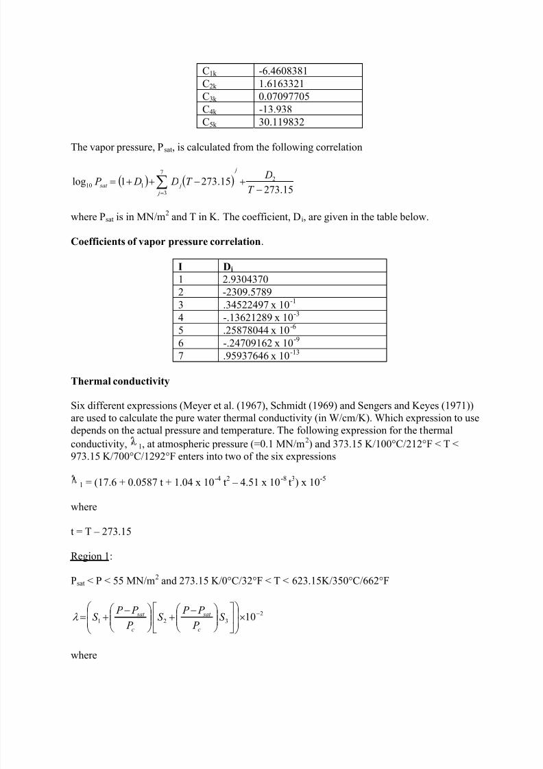
7/18/2019 PVTsim Tutorial Calsep
http://slidepdf.com/reader/full/pvtsim-tutorial-calsep 104/140
C1k -6.4608381C2k 1.6163321C3k 0.07097705C4k -13.938C5k 30.119832
The vapor pressure, Psat, is calculated from the following correlation
( ) ( )15.273
15.2731log 27
3110 −
+−++= ∑= T
DT D D P
j
j
j sat
where Psat is in MN/m2 and T in K. The coefficient, Di, are given in the table below.
Coefficients of vapor pressure correlation.
I Di 1 2.93043702 -2309.57893 .34522497 x 10-1 4 -.13621289 x 10-3 5 .25878044 x 10-6 6 -.24709162 x 10-9 7 .95937646 x 10-13
Thermal conductivity
Six different expressions (Meyer et al. (1967), Schmidt (1969) and Sengers and Keyes (1971))are used to calculate the pure water thermal conductivity (in W/cm/K). Which expression to usedepends on the actual pressure and temperature. The following expression for the thermalconductivity, 1, at atmospheric pressure (=0.1 MN/m2) and 373.15 K/100°C/212°F < T <973.15 K/700°C/1292°F enters into two of the six expressions
1 = (17.6 + 0.0587 t + 1.04 x 10⁻⁴ t2 – 4.51 x 10⁻⁸ t3) x 10-5
where
t = T – 273.15
Region 1:
Psat < P < 55 MN/m2 and 273.15 K/0°C/32°F < T < 623.15K/350°C/662°F
2321 10−×
−+
−+= S
P
P P S
P
P P S
c
sat
c
sat λ
where
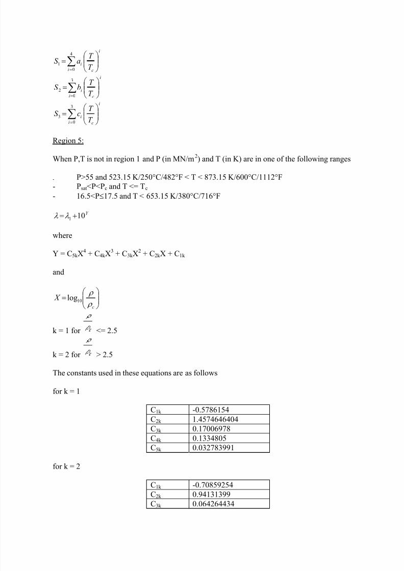
7/18/2019 PVTsim Tutorial Calsep
http://slidepdf.com/reader/full/pvtsim-tutorial-calsep 105/140
∑=
=
4
01
i
i
c
iT
T aS
∑=
=
3
02
i
i
c
iT
T bS
∑=
=
3
03
i
i
c
iT
T cS
Region 5:
When P,T is not in region 1 and P (in MN/m2) and T (in K) are in one of the following ranges
- P>55 and 523.15 K/250°C/482°F < T < 873.15 K/600°C/1112°F
- Psat<P<Pc and T <= Tc
- 16.5<P≤17.5 and T < 653.15 K/380°C/716°F
Y 101 +=λ λ
where
Y = C5k X4 + C4k X
3 + C3k X2 + C2k X + C1k
and
=
c
X ρ ρ 10log
k = 1 for <= 2.5
k = 2 for > 2.5
The constants used in these equations are as follows
for k = 1
C1k -0.5786154C2k 1.4574646404C3k 0.17006978C4k 0.1334805C5k 0.032783991
for k = 2
C1k -0.70859254
C2k 0.94131399C3k 0.064264434
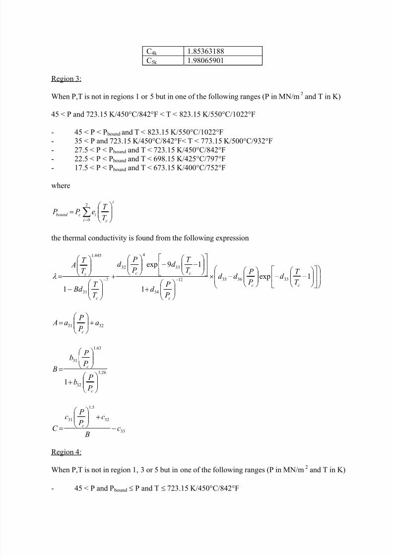
7/18/2019 PVTsim Tutorial Calsep
http://slidepdf.com/reader/full/pvtsim-tutorial-calsep 106/140
C4k 1.85363188C5k 1.98065901
Region 3:
When P,T is not in regions 1 or 5 but in one of the following ranges (P in MN/m2 and T in K)
45 < P and 723.15 K/450°C/842°F < T < 823.15 K/550°C/1022°F
- 45 < P < P bound and T < 823.15 K/550°C/1022°F- 35 < P and 723.15 K/450°C/842°F< T < 773.15 K/500°C/932°F- 27.5 < P < P bound and T < 723.15 K/450°C/842°F- 22.5 < P < P bound and T < 698.15 K/425°C/797°F- 17.5 < P < P bound and T < 673.15 K/400°C/752°F
where
∑=
=
2
0i
i
c
icbound T
T e P P
the thermal conductivity is found from the following expression
−−
−×
+
−−
+
−
= −− 1exp
1
19exp
1
33363512
34
33
4
32
7
31
445.1
cc
c
cc
c
c
T
T d
P
P d d
P P d
T
T d
P
P d
T T Bd
T
T A
λ
3231 a P
P a A
c
+
=
26.3
32
63.1
31
1
+
=
c
c
P
P
b
P
P b
B
33
32
5.1
31
c B
c P
P c
C c −
+
=
Region 4:
When P,T is not in region 1, 3 or 5 but in one of the following ranges (P in MN/m2 and T in K)
- 45 < P and P bound ≤ P and T ≤ 723.15 K/450°C/842°F
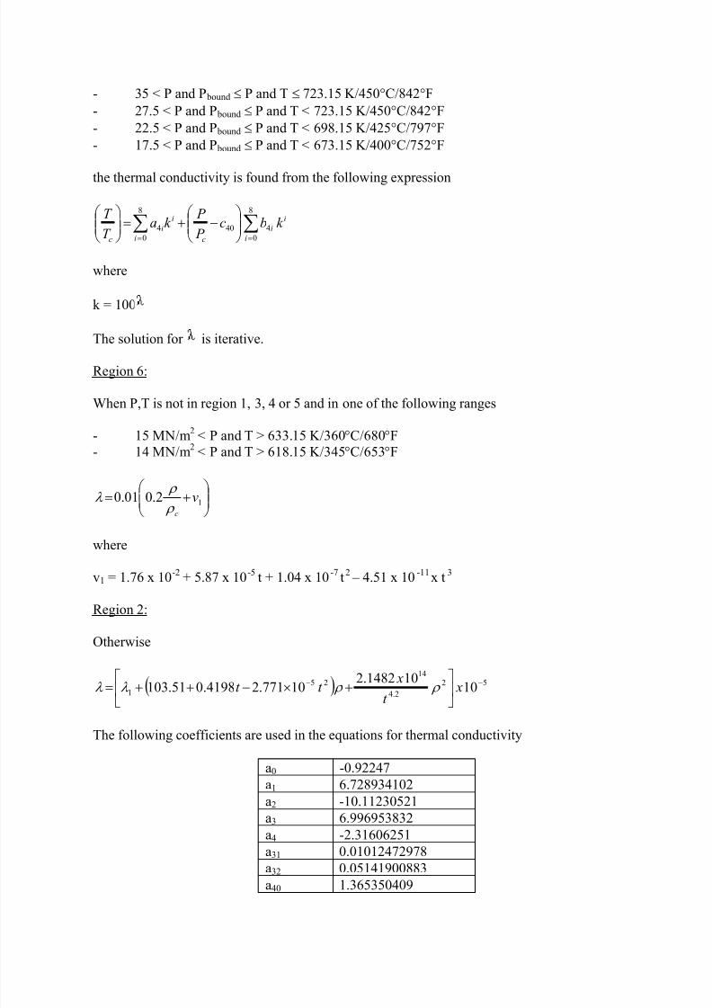
7/18/2019 PVTsim Tutorial Calsep
http://slidepdf.com/reader/full/pvtsim-tutorial-calsep 107/140
- 35 < P and P ≤ P and T ≤ 723.15 K/450°C/842°F bound
- 27.5 < P and P ≤ P and T < 723.15 K/450°C/842°F bound
- 22.5 < P and P bound ≤ P and T < 698.15 K/425°C/797°F- 17.5 < P and P bound ≤ P and T < 673.15 K/400°C/752°F
the thermal conductivity is found from the following expression
where
k = 100
The solution for is iterative.
When P,T is not in region 1, 3, 4 or 5 and in one of the following ranges
- 15 MN/m < P and T > 633.15 K/360°C/680°F2
- 14 MN/m < P and T > 618.15 K/345°C/653°F2
v = 1.76 x 10 + 5.87 x 10 t + 1.04 x 10 t – 4.51 x 10 x t-2 -5 -7
∑ ∑= =
−+=
8
0
8
04404
i i
i
i
c
i
i
c
k bc P
P k a
T
T
Region 6:
+= 12.001.0 v
c ρ
ρ λ
where
12 -11 3
Region 2:
Otherwise
( )52
2.4
1425
110
101482.210771.24198.051.103 −−
+×−++= x
t
xt t ρ ρ λ λ
The following coefficients are used in the equations for thermal conductivity
a0 -0.92247a1 6.728934102a2 -10.11230521a3 6.996953832a4 -2.31606251a31 0.01012472978
a32 0.05141900883a40 1.365350409
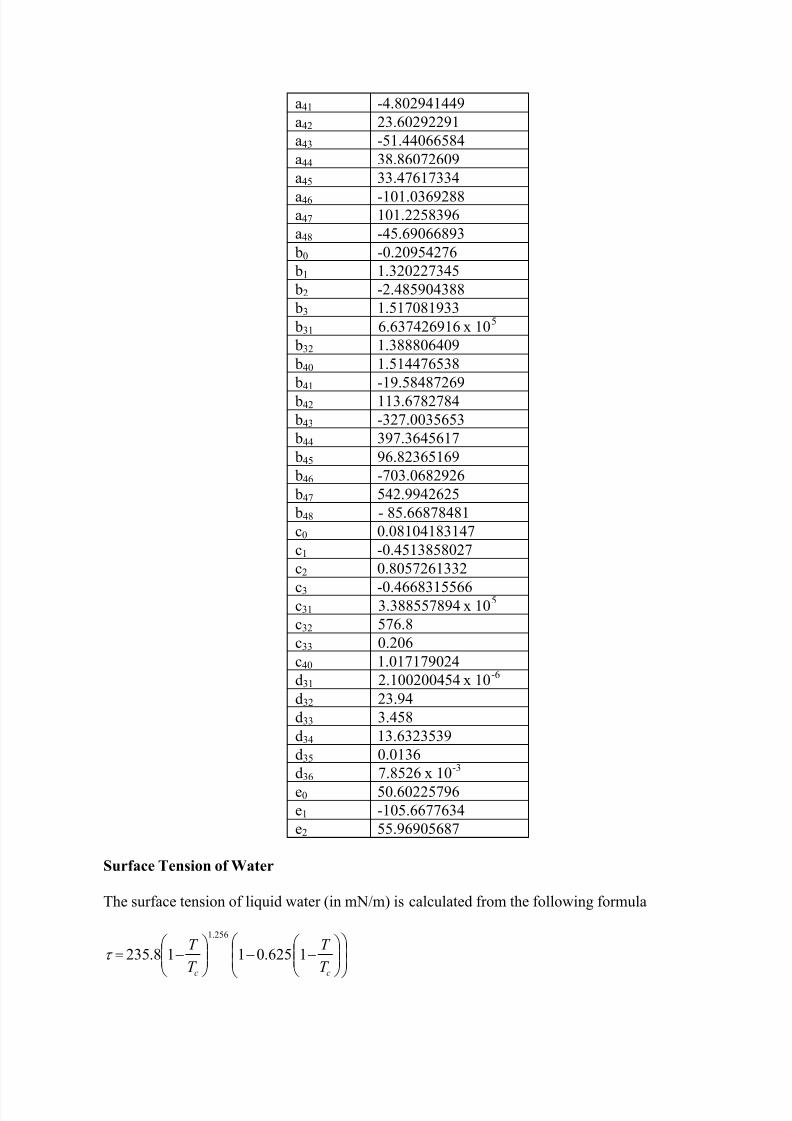
7/18/2019 PVTsim Tutorial Calsep
http://slidepdf.com/reader/full/pvtsim-tutorial-calsep 108/140
a41 -4.802941449a42 23.60292291a43 -51.44066584a44 38.86072609a45 33.47617334
a46 -101.0369288a47 101.2258396a48 -45.69066893
b0 -0.20954276 b1 1.320227345 b2 -2.485904388 b3 1.517081933 b31 6.637426916 x 10⁵ b32 1.388806409 b40 1.514476538
b41 -19.58487269 b42 113.6782784 b43 -327.0035653 b44 397.3645617 b45 96.82365169 b46 -703.0682926 b47 542.9942625 b48 - 85.66878481c0 0.08104183147c1 -0.4513858027c2 0.8057261332c3 -0.4668315566c31 3.388557894 x 10⁵ c32 576.8c33 0.206c40 1.017179024d31 2.100200454 x 10⁻⁶ d32 23.94d33 3.458d34 13.6323539d35 0.0136
d36 7.8526 x 10⁻³ e0 50.60225796e1 -105.6677634e2 55.96905687
Surface Tension of Water
The surface tension of liquid water (in mN/m) is calculated from the following formula
−−
−=
cc T
T
T
T 1625.0118.235
256.1
τ
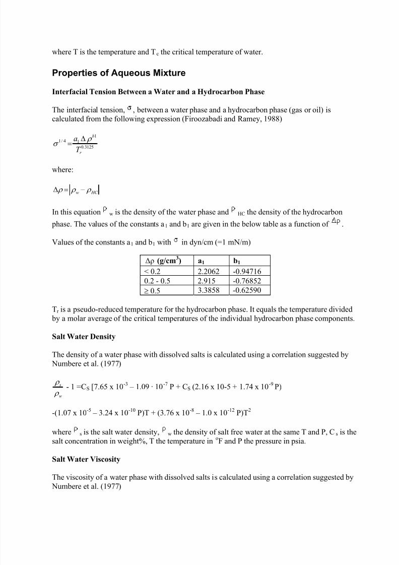
7/18/2019 PVTsim Tutorial Calsep
http://slidepdf.com/reader/full/pvtsim-tutorial-calsep 109/140
where T is the temperature and Tc the critical temperature of water.
Properties of Aqueous Mixture
Interfacial Tension Between a Water and a Hydrocarbon Phase
The interfacial tension, , between a water phase and a hydrocarbon phase (gas or oil) iscalculated from the following expression (Firoozabadi and Ramey, 1988)
3125.0
114/1
r
b
T
a ρ σ
∆=
where:
HC w
ρ ρ ρ −=∆
In this equation w is the density of the water phase and HC the density of the hydrocarbon
phase. The values of the constants a1 and b1 are given in the below table as a function of .
Values of the constants a1 and b1 with in dyn/cm (=1 mN/m)
∆ρ (g/cm3) a1 b1
< 0.2 2.2062 -0.947160.2 - 0.5 2.915 -0.76852
≥ 0.5 3.3858 -0.62590
Tr is a pseudo-reduced temperature for the hydrocarbon phase. It equals the temperature divided by a molar average of the critical temperatures of the individual hydrocarbon phase components.
Salt Water Density
The density of a water phase with dissolved salts is calculated using a correlation suggested by Numbere et al. (1977)
w
s
ρ
ρ
- 1 =CS [7.65 x 10
-3
– 1.09 · 10
-7
P + CS (2.16 x 10⁻⁵ + 1.74 x 10
-9
P)
-(1.07 x 10⁻⁵ – 3.24 x 10⁻¹⁰ P)T + (3.76 x 10⁻⁸ – 1.0 x 10⁻¹² P)T2
where s is the salt water density, w the density of salt free water at the same T and P, Cs is thesalt concentration in weight%, T the temperature in oF and P the pressure in psia.
Salt Water Viscosity
The viscosity of a water phase with dissolved salts is calculated using a correlation suggested by
Numbere et al. (1977)
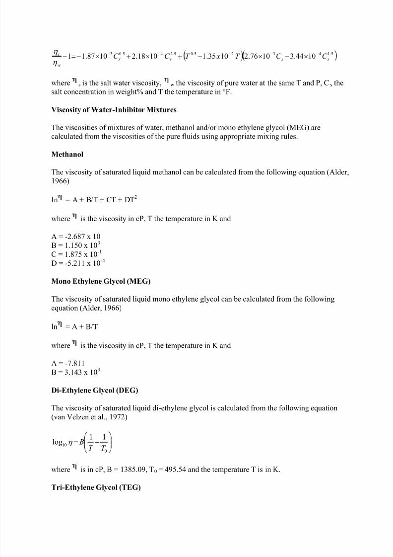
7/18/2019 PVTsim Tutorial Calsep
http://slidepdf.com/reader/full/pvtsim-tutorial-calsep 110/140
( )( )5.14325.05.245.03 1044.31076.21035.11018.21087.11 s s s s
w
s C C T xT C C −−−−− ×−×−+×+×−=−η
η
where s is the salt water viscosity, w the viscosity of pure water at the same T and P, Cs thesalt concentration in weight% and T the temperature in °F.
Viscosity of Water-Inhibitor Mixtures
The viscosities of mixtures of water, methanol and/or mono ethylene glycol (MEG) arecalculated from the viscosities of the pure fluids using appropriate mixing rules.
Methanol
The viscosity of saturated liquid methanol can be calculated from the following equation (Alder,1966)
ln = A + B/T + CT + DT2
where is the viscosity in cP, T the temperature in K and
A = -2.687 x 10B = 1.150 x 10³ C = 1.875 x 10⁻¹ D = -5.211 x 10⁻⁴
Mono Ethylene Glycol (MEG)
The viscosity of saturated liquid mono ethylene glycol can be calculated from the followingequation (Alder, 1966)
ln = A + B/T
where is the viscosity in cP, T the temperature in K and
A = -7.811B = 3.143 x 10³
Di-Ethylene Glycol (DEG)
The viscosity of saturated liquid di-ethylene glycol is calculated from the following equation(van Velzen et al., 1972)
−=
0
10
11log
T T Bη
where is in cP, B = 1385.09, T0 = 495.54 and the temperature T is in K.
Tri-Ethylene Glycol (TEG)
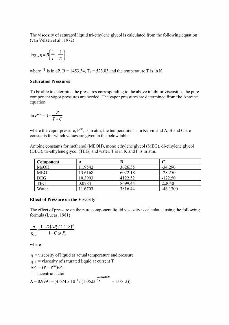
7/18/2019 PVTsim Tutorial Calsep
http://slidepdf.com/reader/full/pvtsim-tutorial-calsep 111/140
The viscosity of saturated liquid tri-ethylene glycol is calculated from the following equation(van Velzen et al., 1972)
−= 010
11
log T T Bη
where is in cP, B = 1453.34, T0 = 523.83 and the temperature T is in K.
Saturation Pressures
To be able to determine the pressures corresponding to the above inhibitor viscosities the purecomponent vapor pressures are needed. The vapor pressures are determined from the Antoineequation
C T
B A P sat
+−=ln
where the vapor pressure, Psat, is in atm, the temperature, T, in Kelvin and A, B and C areconstants for which values are given in the below table.
Antoine constants for methanol (MEOH), mono ethylene glycol (MEG), di-ethylene glycol(DEG), tri-ethylene glycol (TEG) and water. T is in K and P is in atm.
Component A B C
MeOH 11.9542 3626.55 -34.290MEG 13.6168 6022.18 -28.250DEG 10.3993 4122.52 -122.50TEG 0.0784 8699.44 2.2040Water 11.6703 3816.44 -46.1300
Effect of Pressure on the Viscosity
The effect of pressure on the pure component liquid viscosity is calculated using the followingformula (Lucas, 1981)
( )
r
A
r
SL P C
P D
ω η
η
+∆+1
=1
118.2/
where
η = viscosity of liquid at actual temperature and pressure
η SL = viscosity of saturated liquid at current T
r P∆ = (P – Psat)/Pc
ω = acentric factor
A = 0.9991 – (4.674 x 10⁻⁴ / (1.0523 - 1.0513))
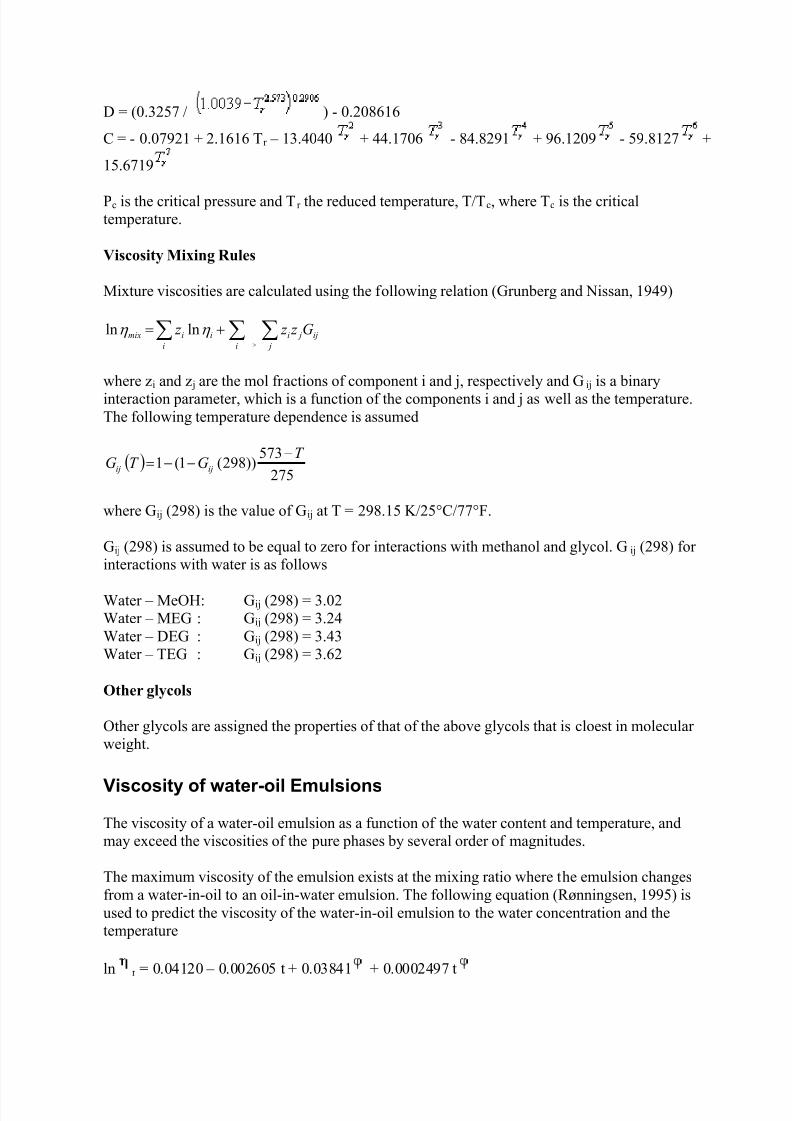
7/18/2019 PVTsim Tutorial Calsep
http://slidepdf.com/reader/full/pvtsim-tutorial-calsep 112/140
D = (0.3257 / ) - 0.208616
C = - 0.07921 + 2.1616 Tr – 13.4040 + 44.1706 - 84.8291 + 96.1209 - 59.8127 +
15.6719
Pc is the critical pressure and Tr the reduced temperature, T/Tc, where Tc is the criticaltemperature.
Viscosity Mixing Rules
Mixture viscosities are calculated using the following relation (Grunberg and Nissan, 1949)
∑ ∑∑>
+=i j
ij ji
i
iimix G z z z η η lnln
where zi and z j are the mol fractions of component i and j, respectively and Gij is a binaryinteraction parameter, which is a function of the components i and j as well as the temperature.The following temperature dependence is assumed
( )275
573))298(1(1
T GT G ijij
−−−=
where Gij (298) is the value of Gij at T = 298.15 K/25°C/77°F.
Gij (298) is assumed to be equal to zero for interactions with methanol and glycol. Gij (298) forinteractions with water is as follows
Water – MeOH: Gij (298) = 3.02Water – MEG : Gij (298) = 3.24Water – DEG : Gij (298) = 3.43Water – TEG : Gij (298) = 3.62
Other glycols
Other glycols are assigned the properties of that of the above glycols that is cloest in molecularweight.
Viscosity of water-oil Emulsions
The viscosity of a water-oil emulsion as a function of the water content and temperature, andmay exceed the viscosities of the pure phases by several order of magnitudes.
The maximum viscosity of the emulsion exists at the mixing ratio where the emulsion changesfrom a water-in-oil to an oil-in-water emulsion. The following equation (Rønningsen, 1995) isused to predict the viscosity of the water-in-oil emulsion to the water concentration and thetemperature
ln r = 0.04120 – 0.002605 t + 0.03841 + 0.0002497 t
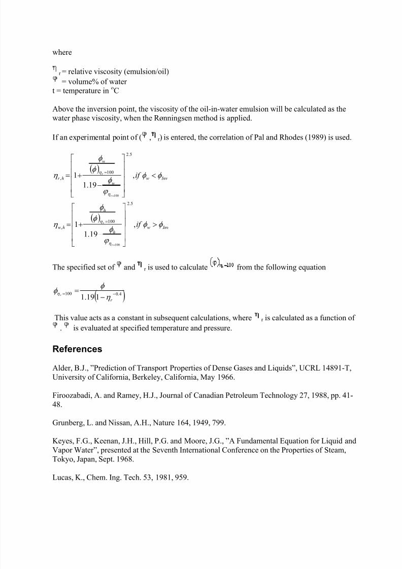
7/18/2019 PVTsim Tutorial Calsep
http://slidepdf.com/reader/full/pvtsim-tutorial-calsep 113/140
where
r = relative viscosity (emulsion/oil)= volume% of water
t = temperature in oC
Above the inversion point, the viscosity of the oil-in-water emulsion will be calculated as thewater phase viscosity, when the Rønningsen method is applied.
If an experimental point of ( , r ) is entered, the correlation of Pal and Rhodes (1989) is used.
( )
( ) Invw
h
h
hw
Invww
w
hr
if
if
r
r
r
r
φ φ
ϕ
φ
φ
φ
η
φ φ
ϕ
φ
φ
φ
η
η
η
η
η
>
−+=
<
−+=
=
=
=
=
,19.1
1
,19.1
1
5.2
100,
5.2
100,
100
100
The specified set of and r is used to calculate from the following equation
( )4.0100 119.1 −= −= r r η
φ
φ η
This value acts as a constant in subsequent calculations, where r is calculated as a function of. is evaluated at specified temperature and pressure.
References
Alder, B.J., ”Prediction of Transport Properties of Dense Gases and Liquids”, UCRL 14891-T,University of California, Berkeley, California, May 1966.
Firoozabadi, A. and Ramey, H.J., Journal of Canadian Petroleum Technology 27, 1988, pp. 41-48.
Grunberg, L. and Nissan, A.H., Nature 164, 1949, 799.
Keyes, F.G., Keenan, J.H., Hill, P.G. and Moore, J.G., ”A Fundamental Equation for Liquid andVapor Water”, presented at the Seventh International Conference on the Properties of Steam,Tokyo, Japan, Sept. 1968.
Lucas, K., Chem. Ing. Tech. 53, 1981, 959.
7/18/2019 PVTsim Tutorial Calsep
http://slidepdf.com/reader/full/pvtsim-tutorial-calsep 114/140
Meyer, C.A., McClintock, R.B., Silverstri, G.J. and Spencer, R.C., Jr., ”Thermodynamic andTransport Properties of Steam, 1967 ASME Steam Tables”, Second Ed., ASME, 1967.
Numbere, D., Bringham, W.E. and Standing, M.B., ”Correlations for Physical Properties ofPetroleum Reservoir Brines”, Work Carried out under US Contract E (04-3) 1265, Energy
Research & Development Administration, 1977.
Pal, R. and Rhodes, E., "Viscosity/Concentration Relationships for Emulsions", J. Rheology,33(7), 1989, 1021.
Rønningsen, H.P., ”Conditions for Predicting Viscosity of W/O Emulsions based on North SeaCrude Oils”, SPE Paper 28968, presented at the SPE International Symposium on OilfieldChemistry, San Antonio, Texas, US, February 14-17, 1995.
Schmidt, E., ”Properties of Water and Steam in SI-Units”, Springer-Verlag, New York, Inc.1969.
Sengers, J.V. and Keyes, P.H., ”Scaling of the Thermal Conductivity Near the Gas-LiquidCritical Point”, Tech. Rep. 71-061, University of Maryland, 1971.
Thomson, G.H. Brabst, K.R. and Hankinson, R.W., AIChE J. 28, 1982, 671.
van Velzen, D., Cordozo, R.L. and Langekamp, H., Ind. Eng. Chem. Fundam. 11, 1972, 20.
7/18/2019 PVTsim Tutorial Calsep
http://slidepdf.com/reader/full/pvtsim-tutorial-calsep 115/140
Modeling of Scale Formation
Modeling of Scale Formation
In the scale module, precipitation is calculated of the minerals BaSO4, SrSO4, CaSO4, CaCO3,
FeCO3 and FeS. The input to the scale module is
• A water analysis, including the concentrations (mg/l) of the inorganic ions Na+, K +, Ca++,Mg++, Ba++, Sr ++, Fe++, Cl-, SO4
-, of organic acid and the alkalinity.
• Contents CO2 and H2S
• Pressure and temperature.
Since the major part of the organic acid pool is acetic acid and since the remaining part behavessimilar to acetic acid, the organic acid pool is taken to be acetic acid.
The alkalinity is defined in terms of the charge balance. If the charge balance is rearranged withall pH-dependent contributions on one side of the equality sign and all pH-independent specieson the other, the alkalinity appears, i.e. the alkalinity is the sum of contributions to the charge
balance from the pH-independent species. Therefore the alkalinity has the advantage ofremaining constant during pH changes.
The calculation of the scale precipitation is based on solubility products and equilibriumconstants. In the calculation, the non-ideal nature of the water phase is taken into account.
Thermodynamic equilibria
The thermodynamic equilibria considered are
• Acid-equilibriaH2O(l) ↔ H+ + OH-
H2O(l) + CO2(aq) ↔ H+ + HCO3--
HCO3- ↔ H+ + CO3
- HA(aq) ↔ H+ + A- H2S(aq) = H+ + HS-
7/18/2019 PVTsim Tutorial Calsep
http://slidepdf.com/reader/full/pvtsim-tutorial-calsep 116/140
• Sulfate mineral precipitation reactionsCa++ + SO4
-- ↔ CaSO4(s)Ba++ + SO4
-- ↔ BaSO4(s)Sr ++ + SO4
-- ↔ SrSO4(s)
• Ferrous iron mineral precipitation reactionsFe++ + CO3
-- ↔ FeCO3 (s)Fe++ + HS- ↔ H+ + FeS(s)
• Calcium carbonate precipitation reactionCa++ + CO3
-- ↔ CaCO3(s)
The thermodynamic equilibrium constants for these reactions are
)(2
2l O H
OH H
OH H O H amm K
−+
−
+=
γ γ
)()(
1
22
3
2
3
2
l O H aqCO
HCO H
CO
HCO H
COam
mm K
γ
γ γ −+−+
=
−
−−+
−
−−+
=3
3
3
3
2 2,
HCO
CO H
HCO
CO H
COm
mm K
γ
γ γ
)()( aq HA
A H
aq HA
A H HA
mmm K
γ γ γ −+−+=
)()( 22
2
aqS H
HS H
aqS H
HS H S H
m
mm K
γ
γ γ −+−+
=
−−++−−++=444 SOCaSOCaCaSO mm K γ γ
−−++−−++=444 SO BaSO Ba BaSO mm K γ γ
−−++−−++=444 SOSr SOSr SrSO mm K γ γ
−−++−−++=333 CO FeCO Fe FeCO mm K γ γ
+
−++
+
−++
= H
HS Fe
H
HS Fe FeS
m
mm K
γ
γ γ
−−++−−++=333 COCaCOCaCaCO
mm K γ γ
7/18/2019 PVTsim Tutorial Calsep
http://slidepdf.com/reader/full/pvtsim-tutorial-calsep 117/140
The temperature dependence of the thermodynamic equilibrium constants is fitted to amathematical expression of the type
( )2
lnlnT
E DT T C
T
B AT K ++++=
A, B, C, D and E for each reaction are listed in the table below.
A B C 1000D E Ref.:
1,2CO K -820.433 50275.5 126.8339 -140.273 -3879660 Haarberg(1989)
2,2CO K -248.419 11862.4 38.92561 -74.8996 -1297999 Haarberg(1989)
HA K -10.937 0 0 0 0
S H K 2
-16.112 0 0 0 0 Østvold
(1998)4CaSO K 11.6592 -2234.4 0 -48.2309 0 Haarberg
(1989)
O H CaSO K 24 2−
815.978 -26309.0 -138.361 167.863 18.6143 Haarberg(1989)
4 BaSO K 208.839 -13084.5 -32.4716 -9.58318 2.58594 Haarberg(1989)
4SrSO K 89.6687 -4033.3 -16.0305 -1.34671 31402.1 Haarberg(1989)
3 FeCO K 21.804 56.448 16.8397 0.02298 0 Østvold
(1998) FeS K -8.3102 0 0 0 0 Østvold
(1998)
3CaCO K -395.448 6461.5 71.558 -180.28 24847 Haarberg(1989)
Coefficients in expression for T-dependence of equilibrium constants. T is in Kelvin.
The temperature dependence of the self-ionization of water is described by Olofsson and Hepler(1982)
( )( ) 21010 0129638.07384.9log195.42296.142613log
2T T T
T T K O H +−+=−
483.890810602.41015068.1 4935 −×+×− −−T T
The pressure dependence is given by
RT
V ZP
P
K i ∆−∆=
∂
∂ ln
Where is the partial molar compressibility change of the reaction, is the partial molar
volume change of the reaction and R is the universal gas constant. for the sulfate precipitation reactions is expressed by a third degree polynomial
7/18/2019 PVTsim Tutorial Calsep
http://slidepdf.com/reader/full/pvtsim-tutorial-calsep 118/140
- 10-3 = a + bt + ct2 + dt3
Where t is the temperature in oC. The coefficients a, b, c and d for each of the sulfate precipitation reactions are listed in the below table
Coefficient in compressibility change expression for sulfate mineral precipitation reactions.Units: t in oC and in cm3 /mol/bar.
a 100b 1000c 106dBaSO4 17.54 -1.159 -17.77 17.06SrSO4 17.83 -1.159 -17.77 17.06CaSO4 16.13 -0.944 -16.52 16.71CaSO4
-2H2O 17.83 -1.543 -16.01 16.84
Reference: Atkinson and Mecik (1997)
The compressibility changes associated with both of the CO2 acid equilibria are (Haarberg, 1989)
233 000371.0233.03.3910102,21,2
T T K Z COCO −+−=∆=∆
For the calcium carbonate and ferrous carbonate precipitation reactions the compressibilitychanges are –0.015 cm3/mol and are considered as independent of temperature (Haarberg et al.,1990).
The partial molar volume changes of the sulfate precipitation reactions are described by theexpression
= A + BT + CT2 + DI + EI2
where I is the ionic strength. The constants A through E for the sulfate mineral precipitationreactions are listed in the below table
Coefficient in volume change expression for sulfate mineral precipitation reactions. Units, T in
Kelvin, I in mols/kg solvent and in cm3/mol.
A B 1000C D EBaSO4 -343.6 1.746 -2.567 11.9 -4SrSO4 -306.9 1.574 -2.394 20 -8.2CaSO4 -282.3 1.438 -2.222 21.7 -9.8CaSO4
-2H2O -263.8 1.358 -2.077 21.7 -9.8
Reference: Haarberg (1989).
For the calcium carbonate and ferrous carbonate precipitation reactions, the partial molar volumechange are described by (Haarberg, 1989)
2002794.0738.17.32833
T T V V FeCOCaCO −+−=∆=∆
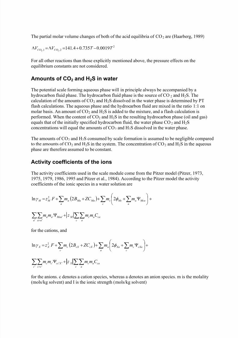
7/18/2019 PVTsim Tutorial Calsep
http://slidepdf.com/reader/full/pvtsim-tutorial-calsep 119/140
The partial molar volume changes of both of the acid equilibria of CO2 are (Haarberg, 1989)
22,1, 0019.0735.04.141
22T T V V COCO −+=∆=∆
For all other reactions than those explicitly mentioned above, the pressure effects on theequilibrium constants are not considered.
Amounts of CO2 and H2S in water
The potential scale forming aqueous phase will in principle always be accompanied by ahydrocarbon fluid phase. The hydrocarbon fluid phase is the source of CO2 and H2S. Thecalculation of the amounts of CO2 and H2S dissolved in the water phase is determined by PTflash calculations. The aqueous phase and the hydrocarbon fluid are mixed in the ratio 1:1 onmolar basis. An amount of CO2 and H2S is added to the mixture, and a flash calculation is
performed. When the content of CO2 and H2S in the resulting hydrocarbon phase (oil and gas)equals that of the initially specified hydrocarbon fluid, the water phase CO2 and H2Sconcentrations will equal the amounts of CO2 and H2S dissolved in the water phase.
The amounts of CO2 and H2S consumed by scale formation is assumed to be negligible comparedto the amounts of CO2 and H2S in the system. The concentration of CO2 and H2S in the aqueous
phase are therefore assumed to be constant.
Activity coefficients of the ions
The activity coefficients used in the scale module come from the Pitzer model (Pitzer, 1973,1975, 1979, 1986, 1995 and Pitzer et al., 1984). According to the Pitzer model the activitycoefficients of the ionic species in a water solution are
( ) +
Ψ++++= ∑ ∑ ∑
a c a
Mcaa Mcc Ma Maa M M mm ZC Bm F z φ γ 22ln 2
∑∑ ∑∑>
+Ψ' '
''a aa c a
caac M Maaaa C mm z mm
for the cations, and
( ) +
Ψ++++= ∑ ∑ ∑
c a c
cXac XaacX cX c X X mm ZC Bm F z φ γ 22ln 2
∑∑ ∑∑>
+Ψ' '
'''c cc c a
caac X X cccc C mm z mm
for the anions. c denotes a cation species, whereas a denotes an anion species. m is the molality(mols/kg solvent) and I is the ionic strength (mols/kg solvent)
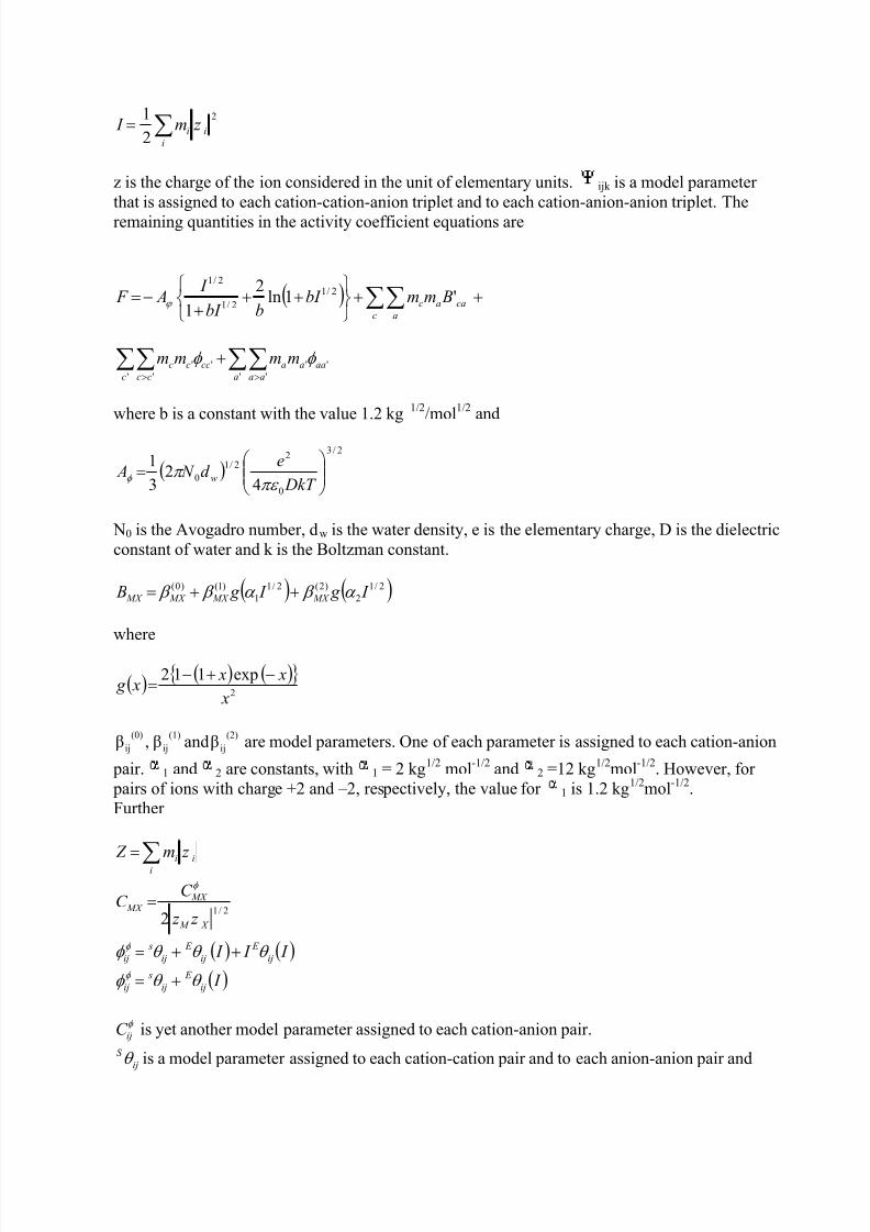
7/18/2019 PVTsim Tutorial Calsep
http://slidepdf.com/reader/full/pvtsim-tutorial-calsep 120/140
∑=i
ii z m I 2
2
1
z is the charge of the ion considered in the unit of elementary units. ijk is a model parameterthat is assigned to each cation-cation-anion triplet and to each cation-anion-anion triplet. Theremaining quantities in the activity coefficient equations are
( ) ∑∑ ++
+++
−=c a
caac BmmbI bbI
I A F '1ln
2
12/1
2/1
2/1
ϕ
∑∑ ∑∑> >
+' ' ' '
''''c cc a aa
aaaacccc mmmm φ φ
where b is a constant with the value 1.2 kg 1/2/mol1/2 and
( )2/3
0
22/1
04
23
1
=
DkT
ed N A w
πε π φ
N0 is the Avogadro number, dw is the water density, e is the elementary charge, D is the dielectricconstant of water and k is the Boltzman constant.
( ) ( )2/12
)2(2/11
)1()0( I g I g B MX MX MX MX α β α β β ++=
where
( ) ( ) ( )
2
exp112
x
x x x g
−+−=
(2)
ij
(1)
ij
(0)
ij βandβ,β are model parameters. One of each parameter is assigned to each cation-anion
pair. 1 and 2 are constants, with 1 = 2 kg1/2 mol-1/2 and 2 =12 kg1/2mol-1/2. However, for pairs of ions with charge +2 and –2, respectively, the value for 1 is 1.2 kg1/2mol-1/2.Further
∑=i
ii z m Z
2/12 X M
MX MX
z z
C C
φ
=
( ) ( ) I I I ij
E
ij
E
ij
s
ij θ θ θ φ φ ++=
( ) I ij
E
ij
s
ij θ θ φ φ +=
φ
ijC is yet another model parameter assigned to each cation-anion pair.
ij
S
θ is a model parameter assigned to each cation-cation pair and to each anion-anion pair and
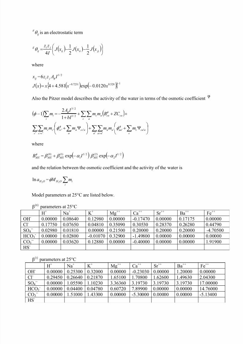
7/18/2019 PVTsim Tutorial Calsep
http://slidepdf.com/reader/full/pvtsim-tutorial-calsep 121/140
ij
E θ is an electrostatic term
( ) ( ) ( )
−−= jjiiij
ji
ij
E x J x J x J I
z z
2
1
2
1
4θ
where
2/16 I A z z x jiij φ =
( ) ( ) ( ) 1528.07231.0 0120.0exp581.44 −− −+= x x x x J
Also the Pitzer model describes the activity of the water in terms of the osmotic coefficient
( ) ( )∑ ∑∑ +++
+
−=−i c a
cacaaci ZC Bmm
bI
I Am φ φ
φ 2/1
2/3
1
21
∑∑ ∑∑ ∑∑> >
Ψ++
Ψ+
' ' ' '''''''
c cc a aa c
acacaaaa
a
accacccc mmmmmm φ φ φ φ
where
( ) ( )2/12
)2(2/11
)1()0( expexp I I B MX MX MX MX α β α β β φ −−+=
and the relation between the osmotic coefficient and the activity of the water is
∑=i
iO H O H m M a22ln φ
Model parameters at 25°C are listed below.
( )0β parameters at 25°C
H Sr + Na+ K + Mg++ Ca++ ++ Ba++ Fe++
OH- 0.00000 0.08640 0.12980 0.00000 -0.17470 0.00000 0.17175 0.00000- 0.17750 0.07650 0.04810 0.35090 0.30530 0.28370 0.26280 0.44790
SO4-- 0.02980 0.01810 0.21500 0.20000 0.20000 0.200000.00000 -4.70500
HCO3
-
0.00000 0.02800 -0.01070 0.32900 -1.49800 0.00000 0.00000 0.00000CO3-- 0.00000 0.03620 0.12880 0.00000 -0.40000 0.00000 0.00000 1.91900
HS-
Cl
(1β ) parameters at 25°C
H+ Na+ K + Mg++ Ca++ Sr ++ Ba++ Fe++
OH- 0.00000 -0.230300.25300 0.32000 0.00000 0.00000 1.20000 0.00000Cl- 0.29450 0.26640 0.21870 1.65100 1.70800 1.62600 1.49630 2.04300SO4
-- 0.00000 1.05590 1.10230 3.36360 3.19730 3.19730 3.19730 17.00000HCO3
- 0.00000 0.04400 0.04780 0.60720 7.89900 0.00000 0.00000 14.76000
CO3
--
0.00000 1.51000 1.43300 0.00000 -5.30000 0.00000 0.00000 -5.13400HS-
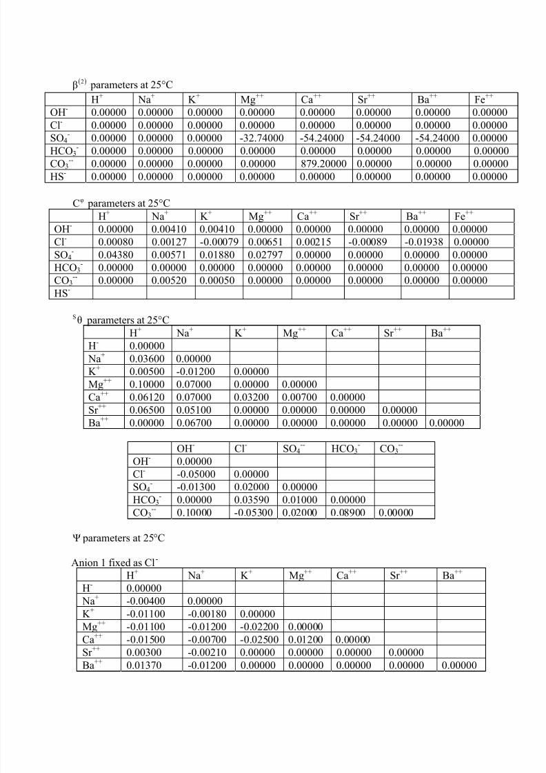
7/18/2019 PVTsim Tutorial Calsep
http://slidepdf.com/reader/full/pvtsim-tutorial-calsep 122/140
( )2β parameters at 25°C
H Mg Ca+ Na+ K + ++ ++ Sr ++ Ba++ Fe++
OH- 0.00000 0.00000 0.00000 0.00000 0.00000 0.00000 0.00000 0.00000Cl- 0.00000 0.00000 0.00000 0.00000 0.00000 0.00000 0.00000 0.00000SO4- 0.00000 0.00000 0.00000 -32.74000 -54.24000 -54.24000 -54.24000 0.00000HCO3
- 0.00000 0.00000 0.000000.00000 0.00000 0.00000 0.00000 0.00000CO3
-- 0.00000 0.00000 0.00000 0.00000 0.000000.00000 879.20000 0.00000- 0.00000 0.00000 0.00000 0.00000 0.00000 0.00000 0.00000 0.00000HS
φC parameters at 25°C
H+ Na+ K + Mg++ Ca++ Sr ++ Ba++ Fe++
OH- 0.00000 0.00410 0.00410 0.00000 0.00000 0.00000 0.00000 0.00000Cl- 0.00080 0.000000.00127 -0.00079 0.00651 0.00215 -0.00089 -0.01938SO4
- 0.04380 0.00571 0.01880 0.02797 0.00000 0.00000 0.00000 0.00000
HCO3- 0.00000 0.00000 0.00000 0.00000 0.00000 0.00000 0.00000 0.00000CO3
-- 0.00000 0.00520 0.00050 0.00000 0.00000 0.00000 0.00000 0.00000HS-
θS parameters at 25°CH+ Na+ K + Mg++ Ca++ Sr ++ Ba++
H- 0.00000 Na+ 0.03600 0.00000K + 0.00500 -0.01200 0.00000Mg++ 0.10000 0.07000 0.00000 0.00000
Ca++
0.06120 0.07000 0.03200 0.00700 0.00000Sr ++ 0.06500 0.05100 0.00000 0.00000 0.00000 0.00000++ 0.06700 0.00000 0.00000 0.00000 0.00000 0.00000Ba 0.00000
OH- Cl- SO4-- HCO3
- CO3--
OH- 0.00000Cl- -0.05000 0.00000
- -0.01300 0.02000 0.00000HCO3
- 0.00000 0.03590 0.01000 0.00000CO3
-- 0.10000 -0.05300 0.02000 0.08900 0.00000
SO4
Ψ parameters at 25°C
HAnion 1 fixed as Cl-
+ Na+ K + Mg++ Ca++ Sr ++ Ba++
H- 0.00000 Na+ -0.00400 0.00000K + -0.01100 -0.00180 0.00000Mg++ -0.01100 -0.01200 -0.02200 0.00000Ca++ -0.01500 -0.00700 -0.02500 0.01200 0.00000Sr ++ 0.00300 -0.00210 0.00000 0.00000 0.000000.00000
Ba++
0.01370 -0.01200 0.00000 0.000000.00000 0.00000 0.00000
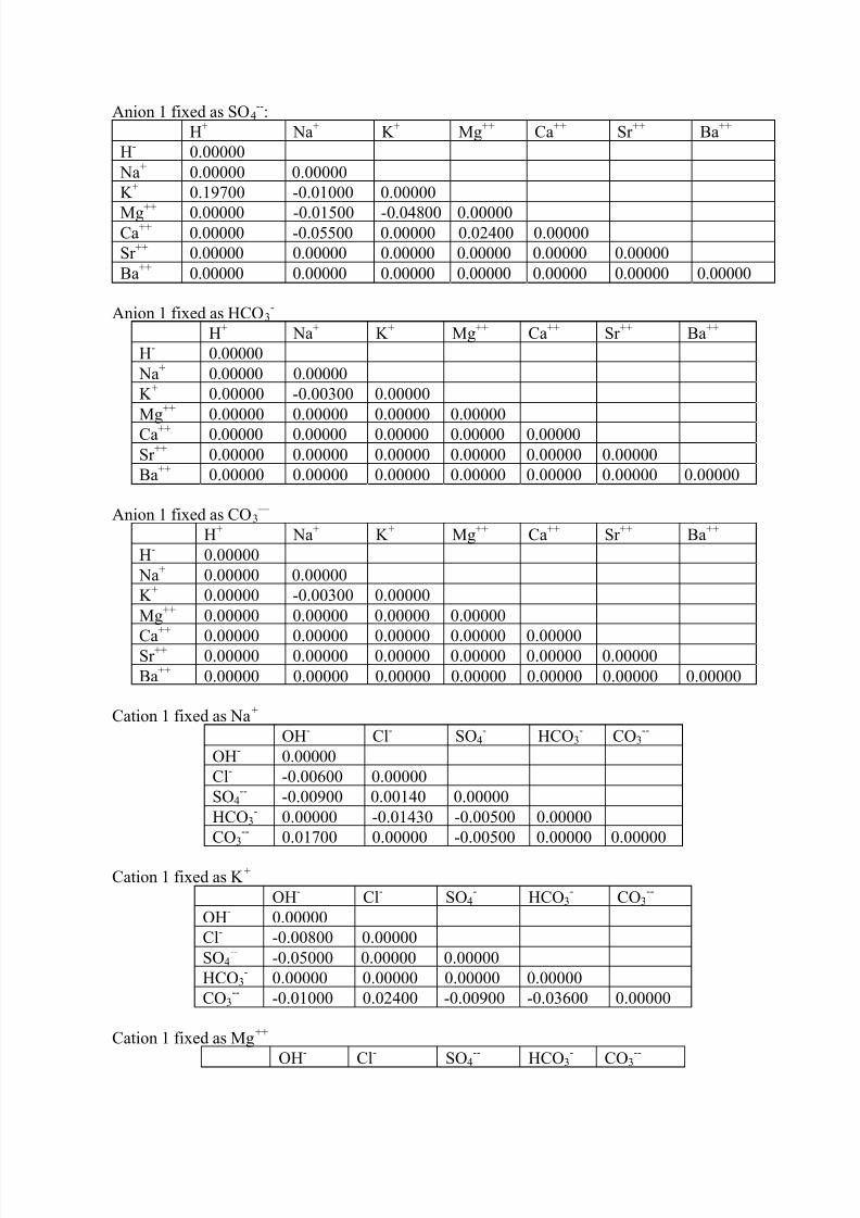
7/18/2019 PVTsim Tutorial Calsep
http://slidepdf.com/reader/full/pvtsim-tutorial-calsep 123/140
Anion 1 fixed as SO4--:
H+ Na+ K + Mg++ Ca++ Sr ++ Ba++
H- 0.00000 Na+ 0.00000 0.00000K + 0.19700 -0.01000 0.00000
Mg 0.00000 -0.04800++ -0.01500 0.00000Ca 0.00000 -0.05500 0.00000++ 0.02400 0.00000Sr ++ 0.00000 0.00000 0.00000 0.00000 0.00000 0.00000Ba++ 0.00000 0.00000 0.00000 0.00000 0.00000 0.00000 0.00000
HAnion 1 fixed as HCO3
- + Na+ K + Mg++ Ca++ Sr ++ Ba++
H- 0.00000 Na+ 0.00000 0.00000K + 0.00000 -0.00300 0.00000
Mg++
0.00000 0.00000 0.00000 0.00000Ca++ 0.00000 0.00000 0.00000 0.00000 0.00000Sr ++ 0.00000 0.00000 0.00000 0.00000 0.00000 0.00000Ba++ 0.00000 0.00000 0.00000 0.00000 0.00000 0.00000 0.00000
Anion 1 fixed as CO H Ba
3 —
+ Na+ K + Mg++ Ca++ Sr ++ ++
H- 0.00000 Na+ 0.00000 0.00000K + 0.00000 -0.00300 0.00000Mg++ 0.00000 0.00000 0.00000 0.00000
Ca++ 0.00000 0.00000 0.00000 0.00000 0.00000Sr ++ 0.00000 0.00000 0.00000 0.00000 0.00000 0.00000Ba++ 0.00000 0.00000 0.00000 0.00000 0.000000.00000 0.00000
Cation 1 fixed as Na+ OH- Cl- SO4
- HCO3- CO3
--
OH- 0.00000Cl- -0.00600 0.00000SO4
-- -0.00900 0.00140 0.00000HCO3
- 0.00000 -0.01430 -0.00500 0.00000
CO3--
0.01700 0.00000 -0.00500 0.00000 0.00000
Cation 1 fixed as K + OH- Cl- SO4
- HCO3- CO3
--
OH- 0.00000Cl- -0.00800 0.00000SO4
-- -0.05000 0.00000 0.00000HCO3
- 0.00000 0.00000 0.00000 0.00000CO3
-- -0.01000 0.02400 -0.00900 -0.03600 0.00000
Cation 1 fixed as Mg++
OH- Cl- SO4-- HCO3
- CO3--
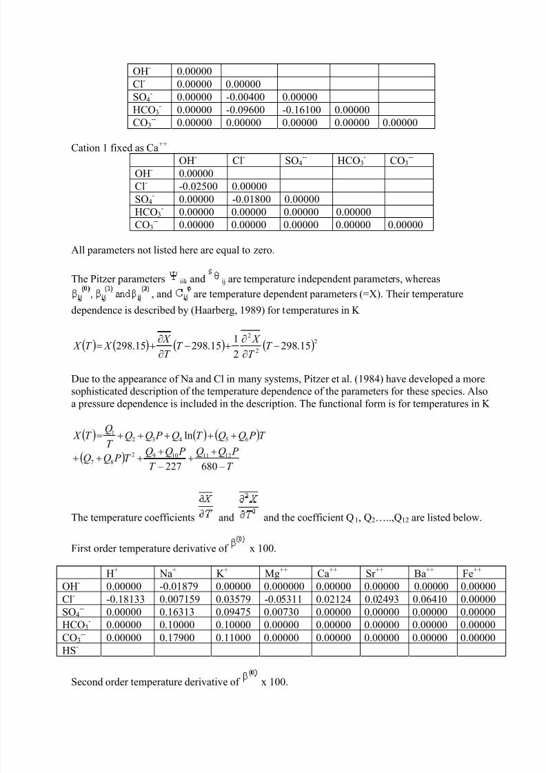
7/18/2019 PVTsim Tutorial Calsep
http://slidepdf.com/reader/full/pvtsim-tutorial-calsep 124/140
OH- 0.00000Cl- 0.00000 0.00000SO4
- 0.00000 -0.00400 0.00000HCO3
- 0.00000 -0.09600 -0.16100 0.00000CO3
-- 0.00000 0.00000 0.00000 0.00000 0.00000
Cation 1 fixed as Ca++ OH- Cl- SO4
-- HCO3- CO3
--
OH- 0.00000Cl- -0.02500 0.00000SO4
- 0.00000 -0.01800 0.00000HCO3
- 0.00000 0.00000 0.00000 0.00000CO3
-- 0.00000 0.00000 0.00000 0.00000 0.00000
All parameters not listed here are equal to zero.
The Pitzer parameters ijk and ij are temperature independent parameters, whereas
, and are temperature dependent parameters (=X). Their temperature
dependence is described by (Haarberg, 1989) for temperatures in K
( ) ( ) ( ) ( )2
2
2
15.2982
115.29815.298 −
∂∂
+−∂∂
+= T T
X T
T
X X T X
Due to the appearance of Na and Cl in many systems, Pitzer et al. (1984) have developed a moresophisticated description of the temperature dependence of the parameters for these species. Alsoa pressure dependence is included in the description. The functional form is for temperatures in K
( ) ( ) ( )T P QQT Q P QQT
QT X 65432
1 ln +++++=
( )T
P QQ
T
P QQT P QQ
−+
+−+
+++680227
1211109287
The temperature coefficients and and the coefficient Q1, Q2…..,Q12 are listed below.
First order temperature derivative of x 100.
H Ca+ Na+ K + Mg++ ++ Sr ++ Ba++ Fe++
OH- 0.00000 -0.01879 0.00000 0.000000 0.00000 0.00000 0.000000.00000Cl- -0.18133 0.007159 0.03579 -0.05311 0.02124 0.02493 0.06410 0.00000SO4
-- 0.00000 0.16313 0.09475 0.00730 0.00000 0.00000 0.00000 0.00000HCO3
- 0.00000 0.10000 0.10000 0.00000 0.00000 0.00000 0.00000 0.00000CO3
-- 0.00000 0.17900 0.11000 0.00000 0.00000 0.00000 0.00000 0.00000-HS
Second order temperature derivative of x 100.
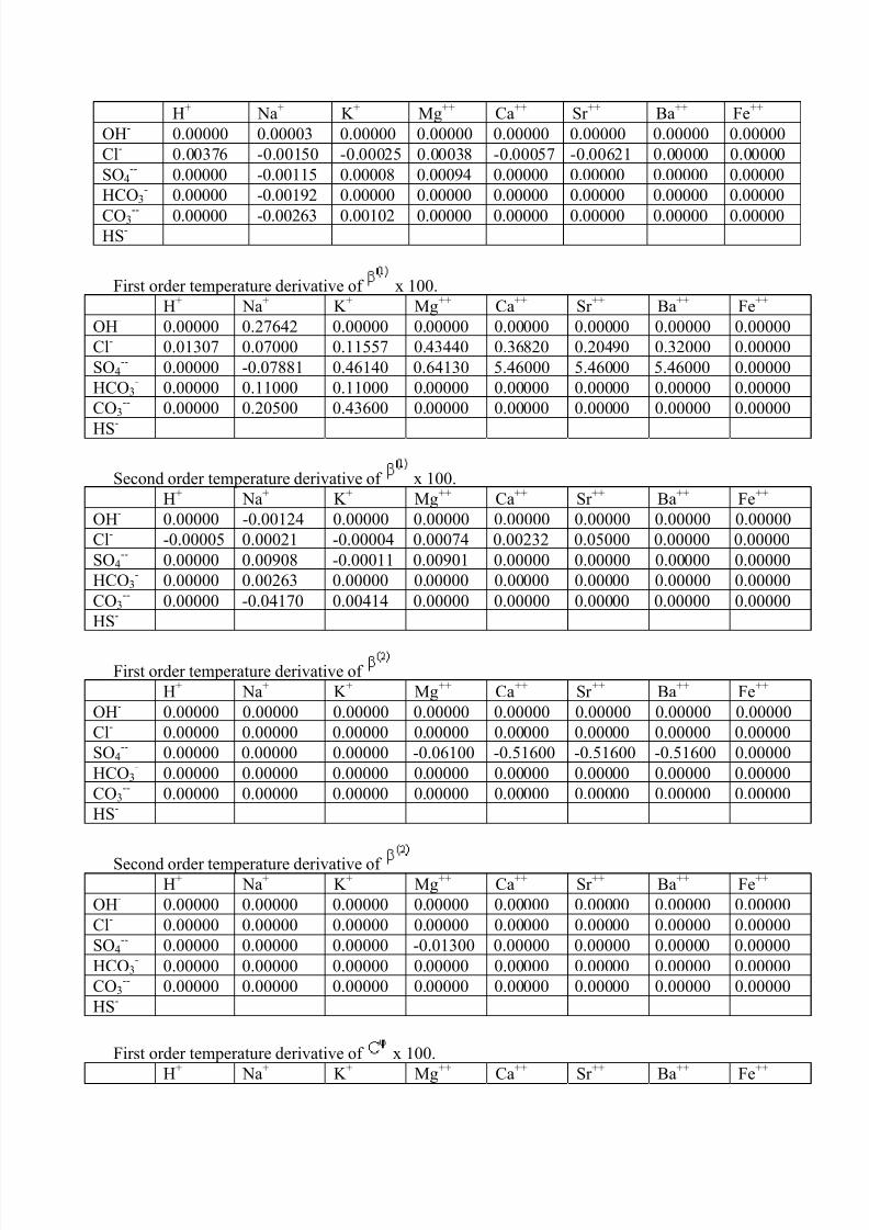
7/18/2019 PVTsim Tutorial Calsep
http://slidepdf.com/reader/full/pvtsim-tutorial-calsep 125/140
H+ Na+ K + Mg++ Ca++ Sr ++ Ba++ Fe++
OH- 0.00000 0.00003 0.00000 0.00000 0.00000 0.00000 0.00000 0.00000Cl- 0.00376 -0.00150 -0.00025 0.00038 -0.00057 -0.00621 0.00000 0.00000SO4
-- 0.00000 -0.00115 0.00008 0.00094 0.00000 0.00000 0.00000 0.00000HCO3
- 0.00000 -0.00192 0.00000 0.00000 0.00000 0.00000 0.00000 0.00000
CO3-- 0.00000 -0.00263 0.00102 0.00000 0.00000 0.00000 0.00000 0.00000HS-
First order temperature derivative of x 100.H Na Mg+ + K + ++ Ca++ Sr ++ Ba++ Fe++
- 0.00000 0.27642 0.00000 0.00000 0.00000 0.00000 0.00000 0.00000Cl- 0.01307 0.07000 0.11557 0.43440 0.36820 0.20490 0.32000 0.00000SO4
-- 0.00000 -0.07881 0.46140 0.64130 5.46000 5.46000 5.46000 0.00000HCO3
- 0.00000 0.11000 0.11000 0.00000 0.00000 0.00000 0.00000 0.00000CO3
-- 0.00000 0.20500 0.43600 0.00000 0.00000 0.00000 0.00000 0.00000
HS-
OH
Second order temperature derivative of x 100.H Na Mg Fe+ + K + ++ Ca++ Sr ++ Ba++ ++
OH- 0.00000 0.00000 0.00000 0.00000 0.00000 0.00000 0.00000-0.00124Cl- -0.00005 0.00021 -0.00004 0.00074 0.00232 0.05000 0.00000 0.00000SO4
-- 0.00000 0.00908 -0.00011 0.00901 0.00000 0.00000 0.00000 0.00000HCO3
- 0.00000 0.00263 0.00000 0.00000 0.00000 0.00000 0.00000 0.00000CO3
-- 0.00000 -0.04170 0.00414 0.00000 0.00000 0.00000 0.00000 0.00000HS-
First order temperature derivative ofH K Mg Ca Sr Fe+ Na+ + ++ ++ ++ Ba++ ++
OH- 0.00000 0.000000.00000 0.00000 0.00000 0.00000 0.00000 0.00000Cl- 0.00000 0.00000 0.00000 0.00000 0.00000 0.00000 0.00000 0.00000SO4
-- 0.00000 0.00000 0.00000 -0.06100 -0.51600 -0.51600 -0.51600 0.00000HCO3
- 0.00000 0.00000 0.00000 0.00000 0.00000 0.00000 0.00000 0.00000
3-- 0.00000 0.00000 0.00000 0.00000 0.00000 0.00000 0.00000 0.00000
HS-CO
Second order temperature derivative ofH+ Na+ K + Mg++ Ca++ Sr ++ Ba++ Fe++
OH- 0.00000 0.00000 0.00000 0.00000 0.00000 0.00000 0.00000 0.00000Cl- 0.00000 0.00000 0.00000 0.00000 0.00000 0.00000 0.00000 0.00000SO4
-- 0.00000 0.00000 0.00000 -0.01300 0.00000 0.00000 0.00000 0.00000HCO3
- 0.00000 0.00000 0.00000 0.00000 0.00000 0.00000 0.00000 0.00000CO3
-- 0.00000 0.00000 0.00000 0.00000 0.00000 0.00000 0.00000 0.00000HS-
First order temperature derivative of x 100.H+ Na+ K + Mg++ Ca++ Sr ++ Ba++ Fe++
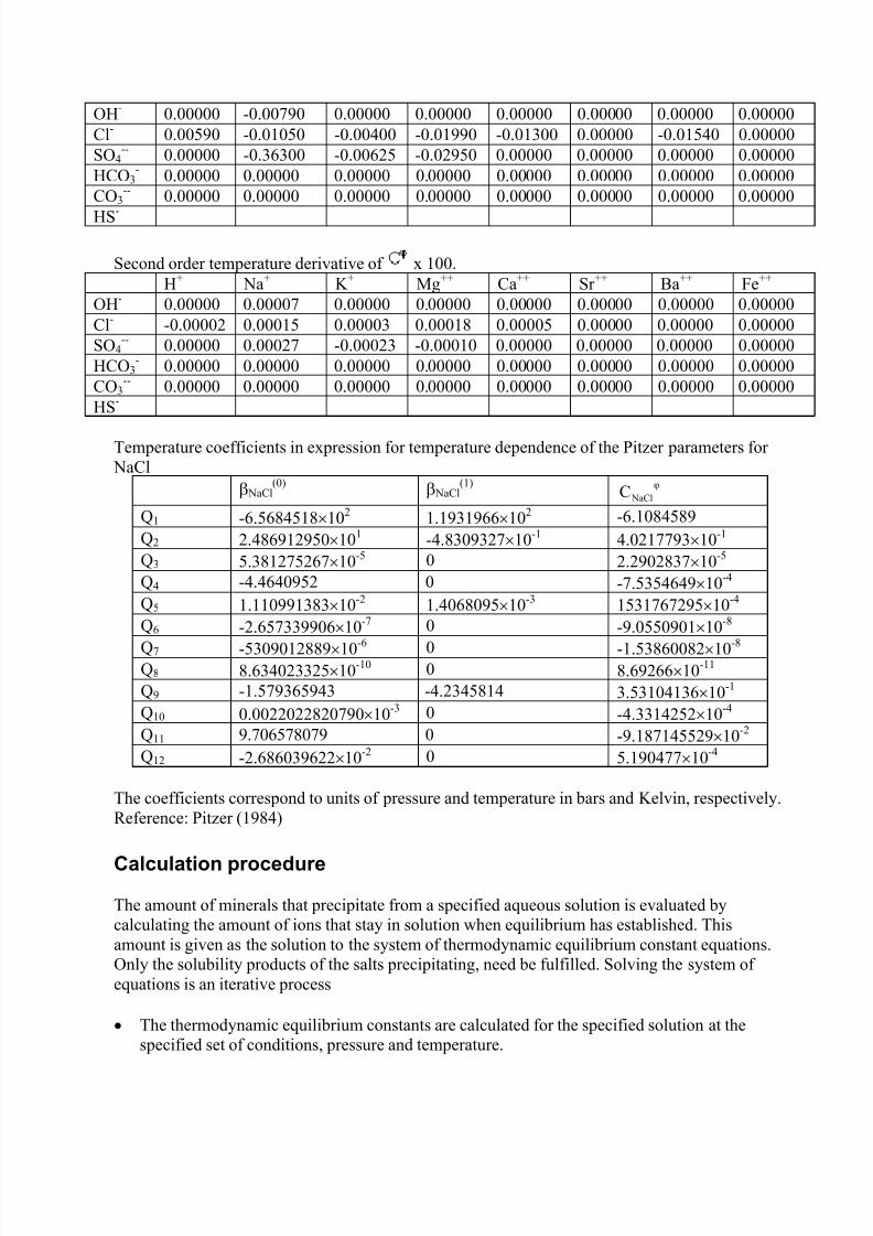
7/18/2019 PVTsim Tutorial Calsep
http://slidepdf.com/reader/full/pvtsim-tutorial-calsep 126/140
OH- 0.00000 -0.00790 0.00000 0.00000 0.00000 0.00000 0.00000 0.00000Cl- 0.00590 -0.01050 -0.00400 -0.01990 -0.01300 0.00000 -0.01540 0.00000SO4
-- 0.00000 -0.36300 -0.00625 -0.02950 0.00000 0.00000 0.00000 0.00000HCO3
- 0.00000 0.00000 0.00000 0.00000 0.00000 0.00000 0.00000 0.00000CO3
-- 0.00000 0.00000 0.00000 0.00000 0.00000 0.00000 0.00000 0.00000
HS-
Second order temperature derivative of x 100.H+ Na+ K + Mg++ Ca++ Sr ++ Ba++ Fe++
OH- 0.00000 0.00007 0.00000 0.00000 0.00000 0.00000 0.00000 0.00000Cl- -0.00002 0.00015 0.00003 0.00018 0.00005 0.00000 0.00000 0.00000SO4
-- 0.00000 0.00027 -0.00023 -0.00010 0.00000 0.00000 0.00000 0.00000HCO3
- 0.00000 0.00000 0.00000 0.00000 0.00000 0.00000 0.00000 0.00000CO3
-- 0.00000 0.00000 0.00000 0.00000 0.00000 0.00000 0.00000 0.00000HS-
Temperature coefficients in expression for temperature dependence of the Pitzer parameters for NaCl
β NaCl(0) β NaCl
(1) φ
NaClC
Q1 -6.5684518×10² 1.1931966×10² -6.1084589Q2 2.486912950×101 -4.8309327×10⁻¹ 4.0217793×10⁻¹
Q3 5.381275267×10⁻⁵ 0 2.2902837×10⁻⁵
Q4 -4.4640952 0 -7.5354649×10⁻⁴
Q5 1.110991383×10⁻² 1.4068095×10⁻³ 1531767295×10-4
Q6 -2.657339906×10⁻⁷ 0 -9.0550901×10⁻⁸
Q7 -5309012889×10-6 0 -1.53860082×10⁻⁸
Q8 8.634023325×10⁻¹⁰ 0 8.69266×10⁻¹¹
Q9 -1.579365943 -4.2345814 3.53104136×10⁻¹
Q10 0.0022022820790×10⁻³ 0 -4.3314252×10⁻⁴
Q11 9.706578079 0 -9.187145529×10⁻²
Q12 -2.686039622×10⁻² 0 5.190477×10⁻⁴
The coefficients correspond to units of pressure and temperature in bars and Kelvin, respectively.Reference: Pitzer (1984)
Calculation procedure
The amount of minerals that precipitate from a specified aqueous solution is evaluated bycalculating the amount of ions that stay in solution when equilibrium has established. Thisamount is given as the solution to the system of thermodynamic equilibrium constant equations.Only the solubility products of the salts precipitating, need be fulfilled. Solving the system ofequations is an iterative process
• The thermodynamic equilibrium constants are calculated for the specified solution at thespecified set of conditions, pressure and temperature.
7/18/2019 PVTsim Tutorial Calsep
http://slidepdf.com/reader/full/pvtsim-tutorial-calsep 127/140
• The activity coefficients of all components are set equal to one.
•
• The ratio of CO his determines if any of the ferrous ironminerals FeCO ill precipitate. Only one can precipitate, since both Hare fixed in concentration, and then the Fe
products at the same time.
•
•
The stoichiometric equilibrium constants are calculated from the thermodynamic ones andfrom the activity coefficients.
2(aq) to H2S(aq) is calculated. T3 and FeS w 2S and CO2
++ concentration cannot fulfil both solubility
• The equilibrium in the acid/base reactions is determined without considering the precipitationreactions. The convergence criterion is that the charge balance must be fulfilled.
• The amount of sulfate precipitation (independent of the acid/base reactions) is calculated,with none of the other precipitation reactions taken into account.
The ion product of the iron mineral identified at a previous step is checked against thesolubility product. If the solubility product is exceeded, the amount of precipitate of the ironmineral is determined. The convergence criterion in this iteration is the charge balance.Precipitation of calcium carbonate is not included in the calculation.
The ion product of calcium carbonate is checked against its solubility product. If thesolubility product is exceeded, simultaneous precipitation of calcium carbonate and the ironmineral is calculated. A double loop iteration is applied. The inner loop: With a givenamount of ferrous iron mineral precipitation (which comes from the outer loop), the amountof calcium carbonate precipitate is determined. During the calcium carbonate precipitation,
the sulfate precipitate is influenced since some Ca++
is removed from the solution. The statein the sulfate system is therefore corrected in each of these inner loop iterations. In the innerloop, the charge balance is used to check for convergence. The outer loop: The iterationvariable is the amount of ferrous iron mineral precipitate. Convergence is achieved when theion product of the ferrous mineral matches the thermodynamic solubility product.
• The resulting amount of each precipitate is compared to that of the previous iteration. If theweighted sum of relative changes in the amounts of precipitates exceeds 10-6, then all activitycoefficients are recalculated from Pitzers activity coefficient model for electrolytes. The
procedure is then repeated from the 3rd step.
References
Atkinson, A. and Mecik, M., “The Chemistry of Scale Prediction”, Journal of Petroleum Scienceand Engineering 17 (1997) pp. 113-121.
Haarberg, T. “Mineral Deposition During Oil Recovery”, Ph.D. Thesis, Department of InorganicChemistry, Trondheim, Norway (1989).
Haarberg, T., Jakobsen, J.E., and Østvold, T., “The effect of Ferrous Iron on Mineral ScalingDuring Oil Recovery”, Acta Chemica Scandinavia 44 (1990) pp. 907-915.
7/18/2019 PVTsim Tutorial Calsep
http://slidepdf.com/reader/full/pvtsim-tutorial-calsep 128/140
Kaasa, B. and Østvold, T., “Prediction of pH and Mineral Scaling in Waters with Varying IonicStrength Containing CO2 and H2S for 0<T(oC)<200 and 1<p(bar)<500” Presented at theconference “Advances in Solving Oilfield Scaling” held January 28 and 29, 1998 in Aberdeen,Scotland.
Pitzer, K.S., “Thermodynamics of Electrolytes I. Theoretical basis and general equations”,Journal of Physical Chemistry 77 (1973) pp. 268-277.
Pitzer, K.S., “Thermodynamics of Electrolytes V. Effects of Higher-Order Electrostatic Terms”,Journal of Solution Chemistry 4 (1975) pp. 249-265.
Pitzer, K.S., “Theory: Ion Interaction Approach. Activity Coefficients in Electrolyte Solutions”,Book by Pytkowicz, R.M., pp. 157-208, CRC Press, Boca Raton, Florida (1979).
Pitzer, K.S., Peiper, J.C. and Busey, R.H., “Thermodynamic Properties of Aqueous SodiumChloride Solutions”. Journal of Physical Chemistry 13 (1984) pp. 1-102.
Pitzer, K.S., “Theoretical Considerations of Solubility with Emphasis on Mixed AqueousElectrolytes”, Pure and Applied Chemistry 58 (1986) pp. 1599-1610.
Pitzer, K.S., “Thermodynamics” 3. edition, McGraw-Hill, Inc. (1995).
7/18/2019 PVTsim Tutorial Calsep
http://slidepdf.com/reader/full/pvtsim-tutorial-calsep 129/140
Wax Deposition Module
Modeling of wax deposition
The wax deposition module, DepoWax, is fundamentally a steady state compositional pipeline
simulator, in which wax deposition on the pipewall is overlaid on the steady state results. Thesteady state approach is chosen because wax deposition is a very slow process relative to typicalresidence times. In the following, the methods of Lindeloff and Krejbjerg (2001 and 2002) usedfor numerical discretization, heat transfer, energy balances, thermodynamic equilibrium, and waxdeposition will be described.
Discretization of the Pipeline into Sections
The simulator is based on an approach where the pipeline is divided into a number of cells. In thefollowing, these will be referred to as segments and sections. Segments are larger entities, which
are user specified in terms of inlet and outlet position in the x-y coordinate space, where x is thehorizontal coordinate and y the vertical.
Each segment consists of a number of sections, the locations of which are generatedautomatically by the program. The user may only affect the selection of the sections by alteringthe maximum section length and maximum temperature drop over a section, which by default areset to 500 m/1640 ft and 5°C/9°F, respectively. Since the temperature of the fluid as it enters intothe pipeline is generally higher than that of the surroundings, the bulk fluid temperature willgenerally exhibit an exponential decline as the fluid passes through the pipeline. Assuming single
phase flow and steady state in the simulation, a temperature profile may be estimated analyticallyfrom the following expression
( )
−−+= x
mC
DU T T T T
p
tot ambinamb x
&
π exp
The equation states that under the above assumptions, the temperature T x at a given position x can
be calculated based on the mass flowrate , the heat capacities C p, the pipeline diameter D, andthe overall heat transfer coefficient U tot . T amb is the ambient temperature, while T in is the fluidtemperature at the pipeline inlet. This expression may be exploited to optimize the discretizationof the pipeline by assigning section lengths in such a way that the temperature only declines a
predefined amount in each section. This results in short section lengths near the inlet, while
sections are longer further down the pipeline where the temperature changes less.
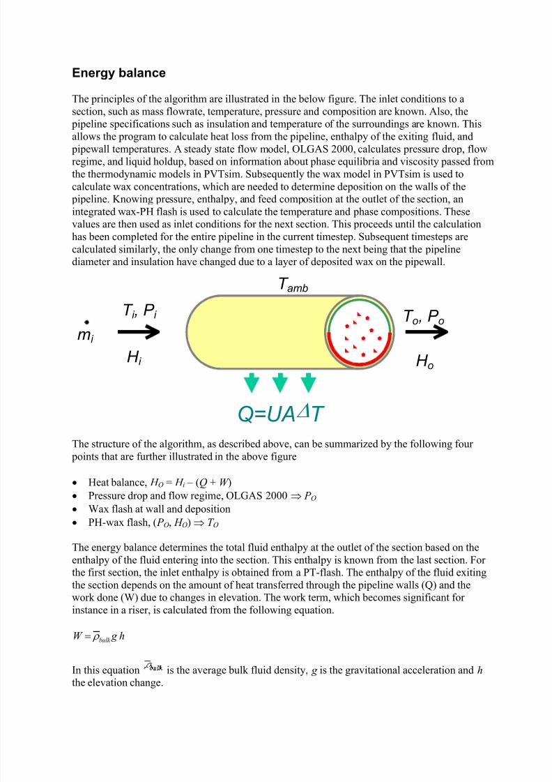
7/18/2019 PVTsim Tutorial Calsep
http://slidepdf.com/reader/full/pvtsim-tutorial-calsep 130/140
Energy balance
The principles of the algorithm are illustrated in the below figure. The inlet conditions to asection, such as mass flowrate, temperature, pressure and composition are known. Also, the
pipeline specifications such as insulation and temperature of the surroundings are known. This
allows the program to calculate heat loss from the pipeline, enthalpy of the exiting fluid, and pipewall temperatures. A steady state flow model, OLGAS 2000, calculates pressure drop, flowregime, and liquid holdup, based on information about phase equilibria and viscosity passed fromthe thermodynamic models in PVTsim. Subsequently the wax model in PVTsim is used tocalculate wax concentrations, which are needed to determine deposition on the walls of the
pipeline. Knowing pressure, enthalpy, and feed composition at the outlet of the section, anintegrated wax-PH flash is used to calculate the temperature and phase compositions. Thesevalues are then used as inlet conditions for the next section. This proceeds until the calculationhas been completed for the entire pipeline in the current timestep. Subsequent timesteps arecalculated similarly, the only change from one timestep to the next being that the pipelinediameter and insulation have changed due to a layer of deposited wax on the pipewall.
Q=UA∆T
T amb
T i , P i
mi
H i H o
T o, P o
The structure of the algorithm, as described above, can be summarized by the following four points that are further illustrated in the above figure
•
•
Heat balance, H O = H i – (Q + W )• Pressure drop and flow regime, OLGAS 2000 ⇒ P O
Wax flash at wall and deposition• PH-wax flash, ( P O, H O) ⇒ T O
The energy balance determines the total fluid enthalpy at the outlet of the section based on theenthalpy of the fluid entering into the section. This enthalpy is known from the last section. Forthe first section, the inlet enthalpy is obtained from a PT-flash. The enthalpy of the fluid exitingthe section depends on the amount of heat transferred through the pipeline walls (Q) and thework done (W) due to changes in elevation. The work term, which becomes significant forinstance in a riser, is calculated from the following equation.
h g W bulk ρ =
In this equation is the average bulk fluid density, g is the gravitational acceleration and h the elevation change.
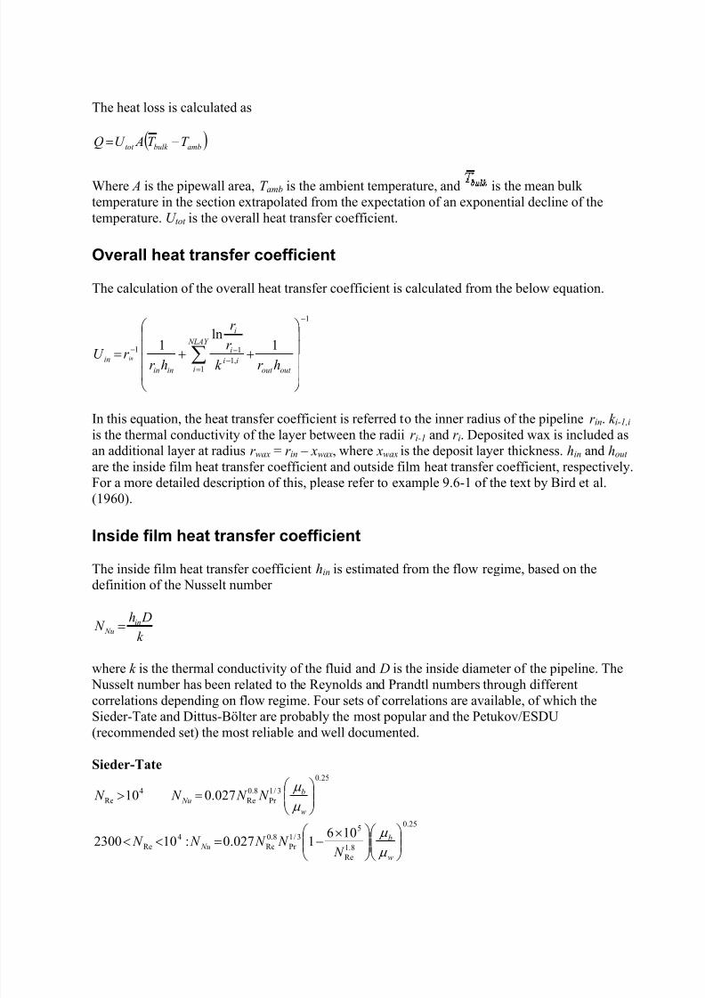
7/18/2019 PVTsim Tutorial Calsep
http://slidepdf.com/reader/full/pvtsim-tutorial-calsep 131/140
The heat loss is calculated as
( )ambbulk tot T T AU Q −=
Where A is the pipewall area, T amb is the ambient temperature, and is the mean bulktemperature in the section extrapolated from the expectation of an exponential decline of thetemperature. U tot is the overall heat transfer coefficient.
Overall heat transfer coefficient
The calculation of the overall heat transfer coefficient is calculated from the below equation.
1
1,111 1
ln1
−
=−
−−
++= ∑ NLAY
i out out
ii
i
i
inin
inhr k
r
r
hr r U in
In this equation, the heat transfer coefficient is referred to the inner radius of the pipeline r in. k i-1,i is the thermal conductivity of the layer between the radii r i-1 and r i. Deposited wax is included asan additional layer at radius r wax = r in – xwax, where xwax is the deposit layer thickness. hin and hout are the inside film heat transfer coefficient and outside film heat transfer coefficient, respectively.For a more detailed description of this, please refer to example 9.6-1 of the text by Bird et al.(1960).
Inside film heat transfer coefficient
The inside film heat transfer coefficient hin is estimated from the flow regime, based on thedefinition of the Nusselt number
k
Dh N in
Nu =
where k is the thermal conductivity of the fluid and D is the inside diameter of the pipeline. The
Nusselt number has been related to the Reynolds and Prandtl numbers through differentcorrelations depending on flow regime. Four sets of correlations are available, of which theSieder-Tate and Dittus-Bölter are probably the most popular and the Petukov/ESDU(recommended set) the most reliable and well documented.
Sieder-Tate25.0
3/1Pr
8.0Re
4Re 027.010
=>
w
b Nu N N N N
µ
µ
25.0
8.1
Re
53/1
Pr 8.0
Re4
Re
1061027.0:102300
×−=<<
w
b Nu
N N N N N
µ
µ
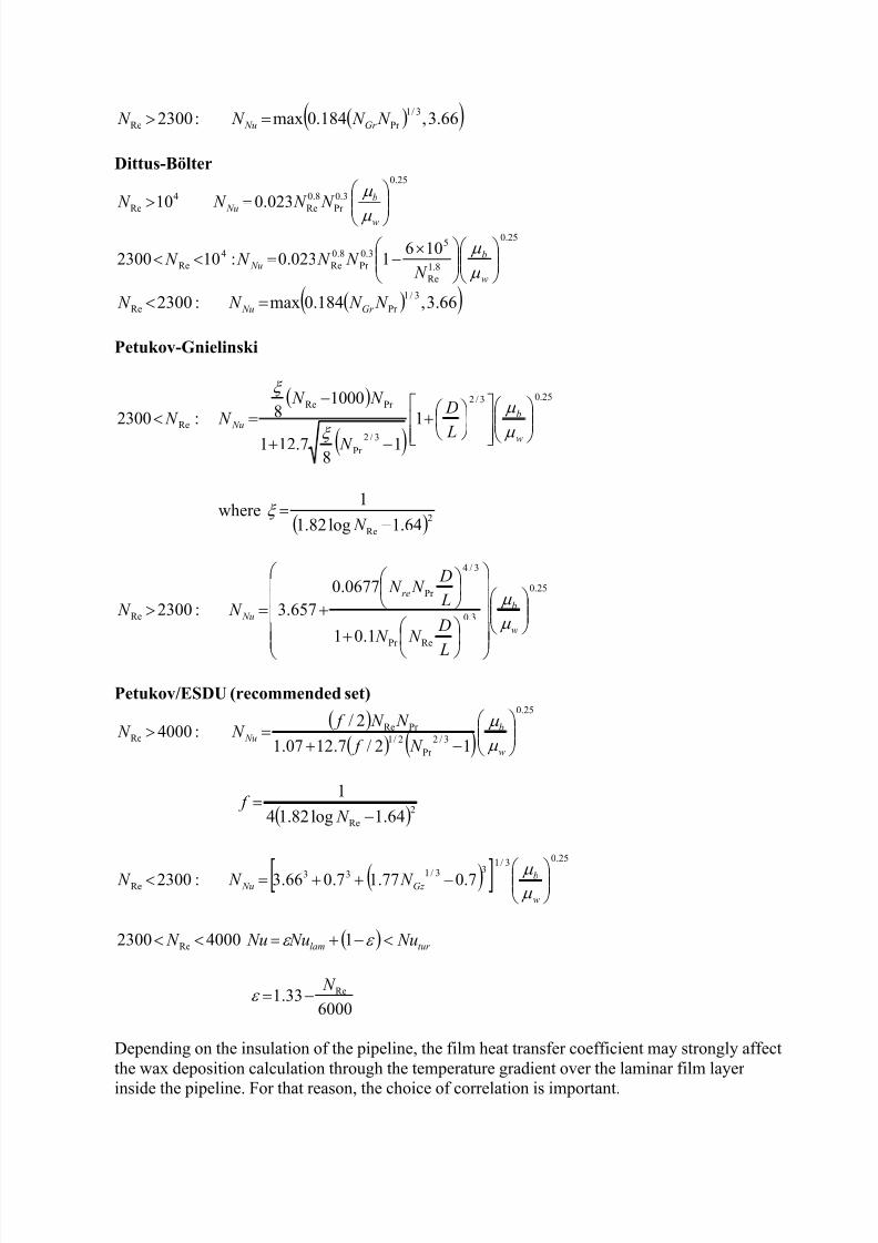
7/18/2019 PVTsim Tutorial Calsep
http://slidepdf.com/reader/full/pvtsim-tutorial-calsep 132/140
( )( )66.3,184.0max:2300 3/1Pr Re N N N N Gr Nu =>
Dittus-Bölter25.0
3.0Pr
8.0Re
4Re 023.010
=>
w
b Nu N N N N
µ
µ
25.0
8.1Re
53.0
Pr 8.0
Re4
Re
1061023.0:102300
×−=<<
w
b Nu
N N N N N
µ
µ
( )( )66.3,184.0max:23003/1
Pr Re N N N N Gr Nu =<
Petukov-Gnielinski
( )
( )
25.03/2
3/2
Pr
Pr Re
Re1
18
7.121
10008:2300
+
−+
−=<
w
b
Nu L
D
N
N N
N N µ
µ
ξ
ξ
where( )2
Re 64.1log82.1
1
− N =ξ
25.0
3.0
RePr
3/4
Pr
Re
1.01
0677.0
657.3:2300
+
+=>w
b
re
Nu
L
D
N N
L
D N N
N N µ
µ
Petukov/ESDU (recommended set)
( )( ) ( )
25.0
3/2Pr
2/1Pr Re
Re12/7.1207.1
2/:4000
−+=>
w
b Nu
N f
N N f N N
µ
µ
( )2
Re 64.1log82.14
1
−=
N f
( )[ ]25.03/1
33/133Re 7.077.17.066.3:2300
−++=<
w
bGz Nu N N N
µ
µ
( ) tur lam Nu Nu Nu N <−+=<< ε ε 140002300 Re
600033.1 Re N
−=ε
Depending on the insulation of the pipeline, the film heat transfer coefficient may strongly affect
the wax deposition calculation through the temperature gradient over the laminar film layerinside the pipeline. For that reason, the choice of correlation is important.
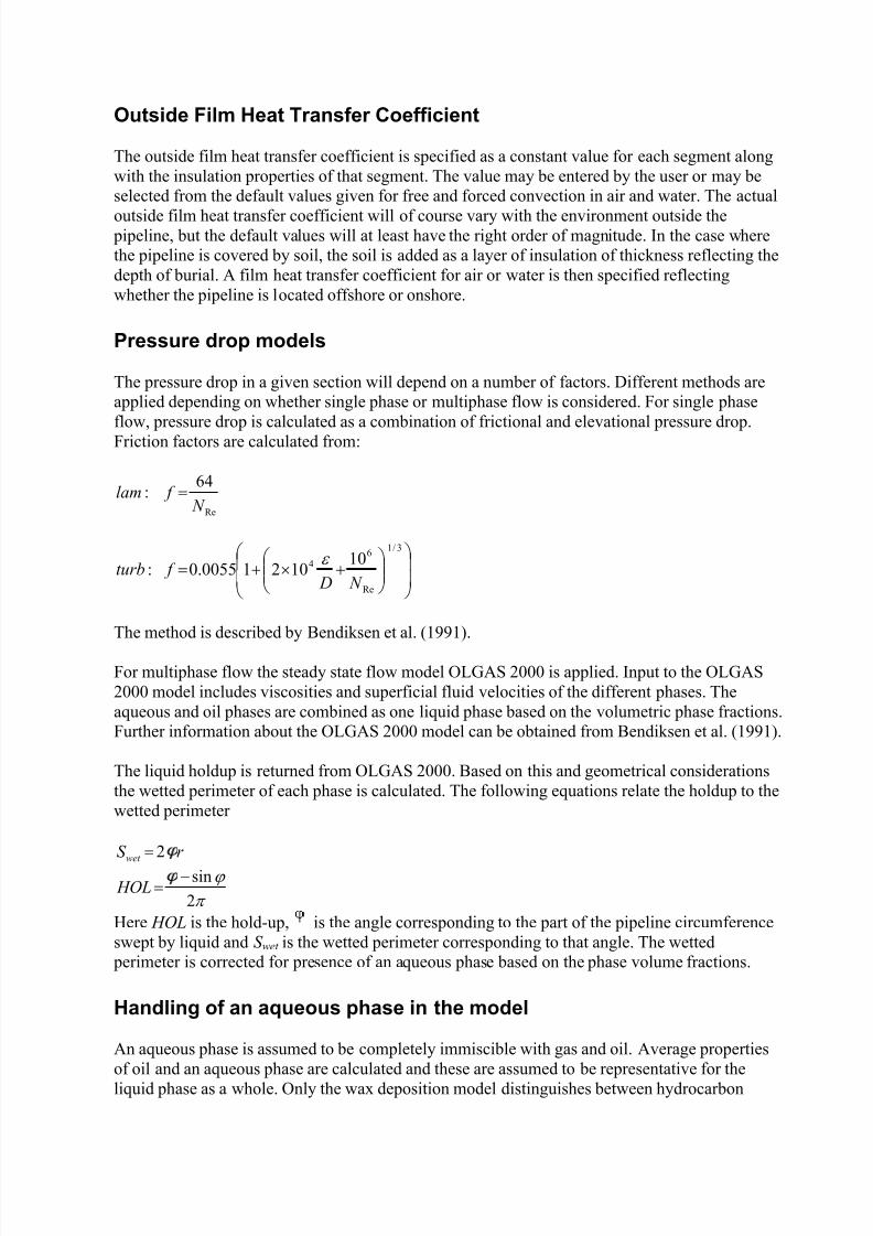
7/18/2019 PVTsim Tutorial Calsep
http://slidepdf.com/reader/full/pvtsim-tutorial-calsep 133/140
Outside Film Heat Transfer Coefficient
The outside film heat transfer coefficient is specified as a constant value for each segment alongwith the insulation properties of that segment. The value may be entered by the user or may beselected from the default values given for free and forced convection in air and water. The actual
outside film heat transfer coefficient will of course vary with the environment outside the pipeline, but the default values will at least have the right order of magnitude. In the case wherethe pipeline is covered by soil, the soil is added as a layer of insulation of thickness reflecting thedepth of burial. A film heat transfer coefficient for air or water is then specified reflectingwhether the pipeline is located offshore or onshore.
Pressure drop models
The pressure drop in a given section will depend on a number of factors. Different methods areapplied depending on whether single phase or multiphase flow is considered. For single phase
flow, pressure drop is calculated as a combination of frictional and elevational pressure drop.Friction factors are calculated from:
Re
64:
N f lam =
+×+=
3/1
Re
64 10
10210055.0: N D
f turb ε
The method is described by Bendiksen et al. (1991).
For multiphase flow the steady state flow model OLGAS 2000 is applied. Input to the OLGAS2000 model includes viscosities and superficial fluid velocities of the different phases. Theaqueous and oil phases are combined as one liquid phase based on the volumetric phase fractions.Further information about the OLGAS 2000 model can be obtained from Bendiksen et al. (1991).
The liquid holdup is returned from OLGAS 2000. Based on this and geometrical considerationsthe wetted perimeter of each phase is calculated. The following equations relate the holdup to thewetted perimeter
r S wet 2=
π
ϕ
2
sin−= HOL
Here HOL is the hold-up, is the angle corresponding to the part of the pipeline circumferenceswept by liquid and S wet is the wetted perimeter corresponding to that angle. The wetted
perimeter is corrected for presence of an aqueous phase based on the phase volume fractions.
Handling of an aqueous phase in the model
An aqueous phase is assumed to be completely immiscible with gas and oil. Average properties
of oil and an aqueous phase are calculated and these are assumed to be representative for theliquid phase as a whole. Only the wax deposition model distinguishes between hydrocarbon
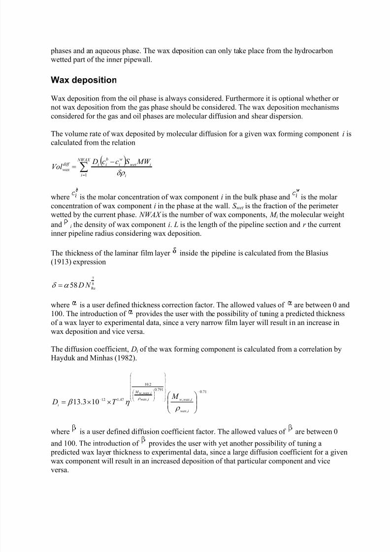
7/18/2019 PVTsim Tutorial Calsep
http://slidepdf.com/reader/full/pvtsim-tutorial-calsep 134/140
phases and an aqueous phase. The wax deposition can only take place from the hydrocarbonwetted part of the inner pipewall.
Wax deposition
Wax deposition from the oil phase is always considered. Furthermore it is optional whether ornot wax deposition from the gas phase should be considered. The wax deposition mechanismsconsidered for the gas and oil phases are molecular diffusion and shear dispersion.
The volume rate of wax deposited by molecular diffusion for a given wax forming component i iscalculated from the relation
( )∑
=
−=
NWAX
i i
iwet
w
i
b
iidiff
wax
MW S cc DVol
1 δρ
where is the molar concentration of wax component i in the bulk phase and is the molarconcentration of wax component i in the phase at the wall. S wet is the fraction of the perimeterwetted by the current phase. NWAX is the number of wax components, M i the molecular weightand i the density of wax component i. L is the length of the pipeline section and r the currentinner pipeline radius considering wax deposition.
The thickness of the laminar film layer inside the pipeline is calculated from the Blasius(1913) expression
8
7
Re58 N Dα δ =
where is a user defined thickness correction factor. The allowed values of are between 0 and100. The introduction of provides the user with the possibility of tuning a predicted thicknessof a wax layer to experimental data, since a very narrow film layer will result in an increase inwax deposition and vice versa.
The diffusion coefficient, Di of the wax forming component is calculated from a correlation byHayduk and Minhas (1982).
71.0
,
,,
791.0
,
,,
2.10
47.112103.13
−
−
××=
iwax
iwaxwiwax
iwaxw M
i
M T D
ρ η β
ρ
where is a user defined diffusion coefficient factor. The allowed values of are between 0
and 100. The introduction of provides the user with yet another possibility of tuning a predicted wax layer thickness to experimental data, since a large diffusion coefficient for a givenwax component will result in an increased deposition of that particular component and viceversa.
7/18/2019 PVTsim Tutorial Calsep
http://slidepdf.com/reader/full/pvtsim-tutorial-calsep 135/140
For systems with a large oil fraction, it is generally expected that deposition is dominated by oil phase deposition to an extent where contributions from the gas phase are negligible. For richgases and lean condensate systems, it may however be of interest to include contributions fromthe gas as well. The model considers wax deposition from the gas phase as results of bothmolecular diffusion and shear dispersion. The same assumptions are used as for the oil phase.
Whether wax deposition from the gas phase should be considered or not is selected on the’Simulation Options’ menu.
Shear dispersion accounts for deposition of wax already precipitated in the bulk phase. Thevolume rate of wax deposited from shear dispersion is estimated from the following correlationof Burger et al. (1981)
wax
wall shear
wax
Ack Vol
ρ
γ *
=
where k *
is a shear deposition rate constant, C wall is the volume fraction of deposited wax in theoil in the bulk, is the shear rate at the wall, A is the surface area available for deposition and
wax is the average density of the wax precipitated in the bulk phase. The shear dispersionmechanism is often assumed to be negligible as compared with molecular diffusion (Brown et al.(1993) and Hamouda (1995)). Therefore the allowed values of k
* is set to [0;0.0001 g/cm2] or[0;0.025 lb/ft2] or [0;0.001 kg/m2].
Boost pressure
It is possible to specify a pressure increase or boost pressure at the entrance of each user
specified segment. The boost pressure may originate from a pump or a compressor, which islocated between two sections.
Porosity
The porosity of the deposited wax is understood as the space between the wax crystals occupied by captured oil. This porosity is reported to be quite significant in many cases (70%) and todepend on the shear rate. The program has the possibility of treating the porosity as a constant orto depend linearly on shear rate. The expression used is:
B A += σ φ
In this expression, is the porosity and the shear rate. The constants A and B are determinedfrom two input data points of shear rate and corresponding porosity. If a constant porosity is to beused, A = 0 and B is the constant porosity value.
Boundary conditions
By boundary conditions is understood the fluid inlet specifications to the pipeline. This includes pressure, temperature, flow rate and fluid composition. One or more boundary conditions may bechanged during the simulation at specified timesteps. In case the inlet composition is to bechanged.
7/18/2019 PVTsim Tutorial Calsep
http://slidepdf.com/reader/full/pvtsim-tutorial-calsep 136/140
Mass Sources
A mass source in this context is understood as a side stream to the pipeline. Mass sources may bedefined to enter in a specified segment inlet in a given timestep. Mass sources cannot bespecified to enter in the first segment. In this case a change of boundary conditions may be
specified instead. Temperature and flow rate of the source are specified. The pressure in thesource is assumed to be equal to that of the fluid at the current position in the pipeline. The fluidcomposition for the source is specified by referring to a fluid in the current fluid database. It is
possible to change conditions for the source in a later timestep, or to change the composition ofthat source. The source composition is mixed into the main pipeline stream, and a PH-flashdetermines the phase distribution and temperature of the mixed stream. This is done by firstdetermining the enthalpy of the source through a PT-flash and then determine the mixtureenthalpy based on the molar flow rates. Fluids entered as sources must be characterized to thesame pseudo-components as the original fluid in the simulation.
References
Bendiksen, K.H., Maines, D., Moe, R., Nuland, S.: SPE 19451, (1991), SPE ProductionEngineering, May, pp. 171-180.
Bird, R.B., Steward, W.E., Lightfoot, E.N., Transport Phenomena, (1960), Wiley, NY. pp. 286-28.
Blasius, H., ”Das Ähnlichkeitsgesetz bei Reibungsvorgängen in Flüssigkeiten”, Forch. Ver. Deut.Ing. 131, 1913.
Brown, T.S., Niesen, V.G. and Erickson, D.P., ”Measurement and Prediction of Kinetics ofParaffin Deposition”, SPE 26548, 68th Annual Technical Conference and Exhibition of SPEHouston, Tx, 3-6 October, 1993.
Burger, E.D., Perkins, T.K. and Striegler, I.H., ”Studies of Wax Deposition in the Trans AlaskaPipeline”, Journal of Petroleum Technology, June 1981, 1975-1086.
ESDU 93018 and 92003: ”Forced convection heat transfer in straight tubes”, ESDU 1993.
Hamouda, A., ”An Approach for Simulation of Paraffin Deposition in Pipelines as a Function ofFlow Characteristics with a Reference to Teeside Oil Pipeline”, SPE 28966 (1995), presented at
SPE Int. Symposium on Oilfield Chemistry, San Antonio, 14-17 February 1995.
Hayduk, W. and Minhas, B.S., ”Correlations for Predictions of Molecular Diffusivities inLiquids”, The Canadian Journal of Chemical Engineering, 60, 1982, pp. 295-299.
Lindeloff, N. and Krejbjerg, K., “Compositional Simulation of Wax Deposition in Pipelines:Examples of Application”, Presented at Multiphase ’01, Cannes, France, June 13-15, 2001.
Lindeloff, N. and Krejbjerg, K., “A Compositional Model Simulating Wax Deposition inPipeline Systems”, Energy & Fuels, 16, pp. 887-891, 2002.
7/18/2019 PVTsim Tutorial Calsep
http://slidepdf.com/reader/full/pvtsim-tutorial-calsep 137/140
Szilas, A.P.: ”Production and Transport of Oil and Gas, part B”, 2. Ed. Developments inPetroleum Science, 18B, (1986), Elsevier, Amsterdam.
7/18/2019 PVTsim Tutorial Calsep
http://slidepdf.com/reader/full/pvtsim-tutorial-calsep 138/140
Clean for Mud
Clean for Mud
Reservoir samples are often contaminated by base oil from drilling mud. The Mud module of
PVTsim has been implemented for the purpose of estimating the composition of a reservoir fluidfrom the composition of the fluid with a certain content of base oil contaminate.
It is possible to make regression to experimental PVT data for a contaminated fluid andafterwards make use of the regressed component parameters for the non-contaminated fluid.
Cleaning Procedure
In order to use the Mud module, the following compositional data are needed•
•
Composition of contaminated reservoir fluid. It is customary to analyze to either C7+, C10+,
C20+, or C36+.Composition of base oil contaminate. It will usually consist of components in the carbonnumber range C11 – C30.
• Weight% contaminate in stock tank oil (optional for compositions to C36+)
The cleaning procedure will differ depending on the extent of the compositional analysis
Reservoir fluids to C7+ or C10+
The base oil contaminate will seldom contain components lighter than C11. With a composition toC7+ or C10+ all base oil contaminate will be contained in the plus fraction of the contaminatedreservoir fluid. The base oil affects molar amount, density and molecular weights of the plus
fraction. The weight% contaminate in the oil from a flash of the contaminated reservoir fluid tostandard conditions is required input.
1. Characterization of contaminated reservoir fluid as for a usual plus composition.2. PT-flash to standard conditions3. Weight% contaminate of total reservoir fluid initially estimated as weight% contaminate
of the STO oil (input) multiplied by the weight fraction of oil from flash.4. Contaminated reservoir fluid cleaned.5. Usual characterization of cleaned fluid.6. Weaving of cleaned fluid with mud contaminate.7. PT flash to standard conditions. Check whether calculated amount of contaminate in STO
oil agrees with input. Otherwize make new estimate of eeight% contaminate in reservoirfluid and return to 4.
Chapter 1 Clean for Mud 137
7/18/2019 PVTsim Tutorial Calsep
http://slidepdf.com/reader/full/pvtsim-tutorial-calsep 139/140
Reservoir fluids to C20+
Most base oil contaminates will contain components lighter than C20 as well as componentsheavier than C20. Some contaminate is therefore contained in the plus fraction and some in thelighter fractions. It is practical to have all the contaminate contained in the plus fraction before
performing the cleaning calculation. The carbon number fractions with contaminate are thereforecombined into a plus fraction ending at the carbon number of the lightest base oil component.Say the base oil composition starts at C15, the C15 – C20+ fractions of the contaminated reservoirfluid are combined into a C15+
fraction.
After the contraction of the contaminated reservoir fluid composition the cleaning procedure isthe same as for a C7+ or a C10+ composition.
Reservoir fluids to C36+
With a composition to C36+ the carbon number fraction C7-C10 will usually be free ofcontamination and the same will be the case for the fractions C30-C36. This allows the degree of
contamination to be estimated.
For a clean reservoir fluid PVTsim assumes the following relation between the mol fraction (z)of C7+ fractions and carbon number i.
ii CN B A z ×+=ln
A and B are estimated by a fit to mol%’s for C7+ mol fractions against carbon number.
The above relation will not apply for fractions contaminated by base oil, but it will still be true
for uncontaminated C7+ fractions. A and B may be determined by a linear fit to zi versus CNi,where i stands for uncontaminated C7+ fractions. Using A and B, the mol fractions of theremaining C7+ fractions in the uncontaminated fluid may be estimated. The remaining molaramount of each carbon number fraction is assumed to originate from the base oil, which enablesthe composition of the contaminate to be estimated. The estimated base oil composition will notnecessarily be identical to the input composition.
Cleaning with Regression to PVT Data
Any PVT data will be for the contaminated sample. It is obviously of more interest to know thePVT properties of the uncontaminated fluid. It is therefore desirable to have the option to carryout a regression for the contaminated composition and afterwards be able to apply the regressedcomponent parameters for the uncontaminated fluid.
The contaminated composition is initially cleaned as above. A regression is performed as for ausual plus fraction composition, where the cleaned reservoir fluid composition in each iterativestep is weaved with the base oil contaminate in the pertinent weight ratio. Weaving is a mixingwhere each component of the individual fluids is retained. The base oil contaminate is lumpedinto pseudo-components (default is 4 pseudo-components). Only the components originatingfrom the cleaned reservoir fluid are regressed on, i.e. the base oil components are left out of the
regression. The weaving procedure is selected because it enables regression to be performeddirectly on the component properties of the reservoir fluid.
Chapter 1 Clean for Mud 138
7/18/2019 PVTsim Tutorial Calsep
http://slidepdf.com/reader/full/pvtsim-tutorial-calsep 140/140
Regression on the characterized contaminated fluid is also an option, in which case the sameregression parameters are used as with ordinary regression for characterized fluids. To allow the
program to identify the mud components in the contaminated fluids, the characterized mud must be saved in the database prior to the regression and selected as mud comtaminate in the Clean for
Mud menu. The result of the regression is a cleaned, tuned and characterized reservoir fluidcomposition.