Embed Size (px)
Citation preview
PUSHING THE FRONTIERS OF
SUPERCONDUCTING RADIO FREQUENCY
SCIENCE: FROM THE TEMPERATURE
DEPENDENCE OF THE SUPERHEATING FIELD
OF NIOBIUM TO HIGHER-ORDER MODE
DAMPING IN VERY HIGH QUALITY FACTOR
ACCELERATING STRUCTURES
A Dissertation
Presented to the Faculty of the Graduate School
of Cornell University
in Partial Fulfillment of the Requirements for the Degree of
Doctor of Philosophy
by
Nicholas Ruben Alexander Valles
January 2014

c© 2014 Nicholas Ruben Alexander Valles
ALL RIGHTS RESERVED
PUSHING THE FRONTIERS OF SUPERCONDUCTING RADIO
FREQUENCY SCIENCE: FROM THE TEMPERATURE DEPENDENCE OF
THE SUPERHEATING FIELD OF NIOBIUM TO HIGHER-ORDER MODE
DAMPING IN VERY HIGH QUALITY FACTOR ACCELERATING
STRUCTURES
Nicholas Ruben Alexander Valles, Ph.D.
Cornell University 2014
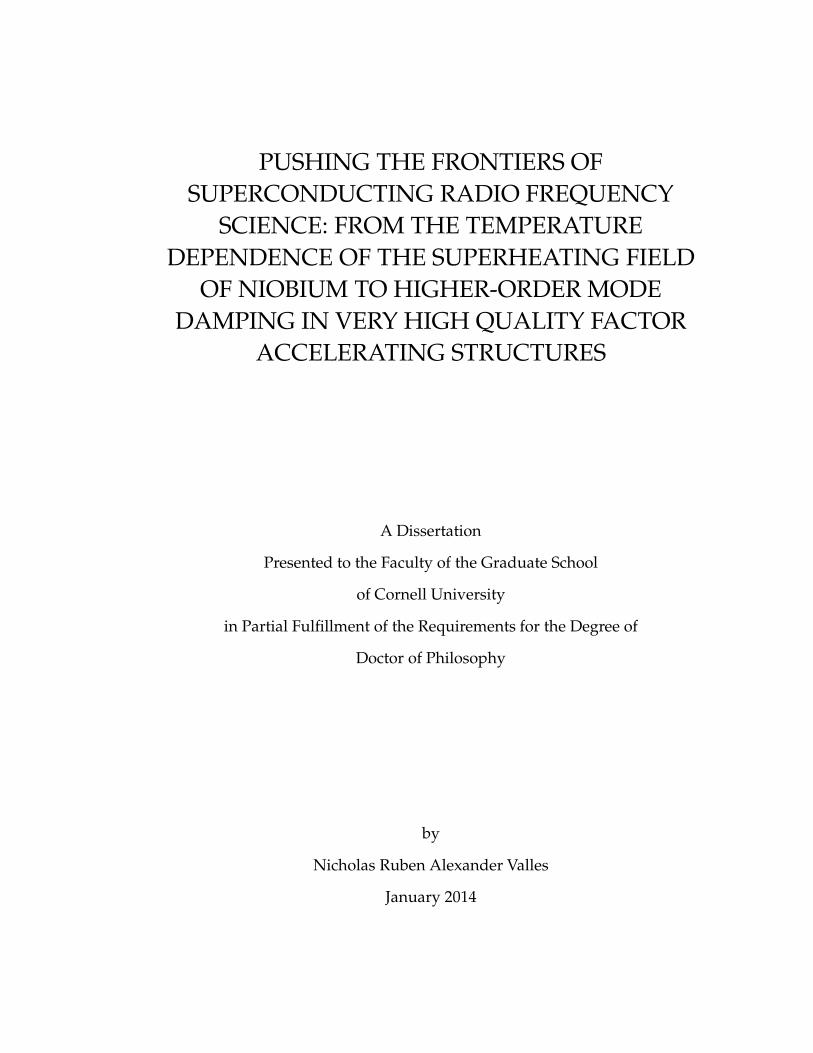
This thesis investigates the three frontiers of superconducting radio frequency
(SRF) science: Gradient, Continuous wave beam power, and High quality factor
structures. On the first front, the full temperature dependence of the superheat-
ing field - which sets the ultimate gradient limit for SRF cavities was measured
for the first time for niobium. It was found that the Ginsburg-Landau result near
Tc is consistent with measurements within measurement uncertainty to even
low temperatures. The beam power frontier was extended by designing a mul-
ticell cavity for the Cornell Energy Recovery Linac (ERL) with strongly damped
higher-order modes. Simulations show that an ERL constructed of these cavi-
ties can support high beam current in excess of 300 mA, ∼30 times higher than
in ERLs currently in operation. Finally, measurements of the prototype main
linac cavity for the Cornell ERL demonstrate that the fundamental accelerating
mode of the cavity in a fully equipped cryomodule can achieve quality factors in
excess of 6×10¹⁰ at 1.8 K and 16.2 MV/m, a result more than tripling the design
specification. This prototype structure also set a world record of Q0 = 1× 10¹¹ at
1.6 K, for a cavity installed in a fully equipped cryomodule, and introduces the
possibility of a new class of extremely high efficiency SRF accelerators.
BIOGRAPHICAL SKETCH
Nick was born at a young age in Berrien Springs, Michigan. He spent his youth
in Southern California until entering Andrews University where he completed
his B.S. in Physics and B.S. in Mathematics in 2008. He earned his M.S. in Physics
at Cornell University in 2011 and finished his Ph.D. in Physics in 2013.
Along the way, he met and married a lovely lady named Anneke and they
are now living in Southern California.
iii

To my wife, Anneke, who is my constant companion through life’s adventures.
iv

ACKNOWLEDGEMENTS
No man is an island
- John Donne
I would like begin my acknowledgements by honoring the memory of Kathy.
I hope that this thesis serves as a small tribute to the mysteries she might have
unraveled.
The document you are reading would not exist without a large investment
of time and effort from many, many people.
I would like to thank, my wife, Anneke, who has been by my side through-
out this process. Any of my accomplishments are a direct result of her continual
support. I also appreciate my parents, grandparents and family members for
stressing the importance of education and teaching, challenging, and support-
ing me through my intellectual journey.
A deep thanks goes to Ozzie Nevarez, who inspired my nascent interest in
physics, and the professors at Andrews University who cultivated my abilities.
My adviser, Matthias Liepe, deserves immeasurable appreciation for his pa-
tience, guidance, stunning physical insight, encyclopedic knowledge of the uni-
verse of SRF, and persistence in forming me into the physicist I am today. Un-
doubtedly, my graduate school career would not have been a success without
him.
Zachary Conway also deserves special recognition for taking me under his
wing as a fledgling graduate student and teaching me the techniques necessary
to conduct SRF research, as does Valery Shemelin for our many fruitful discus-
sions about electromagnetic simulations.
My graduate student colleagues and friends Sam Posen, Dan Gonnella,
Daniel Hall and Yi Xie, who served as fellow researchers in training, lunchtime
v

debate partners and competitors in innumerable1 games of Glory to Rome made
my graduate experience at Cornell a full one, as did the friendship of the
Adams, Sutter and Liepe families.
I would also like to recognize my committee members, James Sethna and
David Rubin, as well as the many technicians, researchers and professors I have
worked with on the Cornell Energy Recovery Linac Test Horizontal Test Cry-
omodule program: Adam Bartnik, Ivan Bazarov, Sergey Belomestnykh, Mike
Billing, Paul Bishop, Benjamin Bullock, Eric Chojnacki, Brian Clasby, James Crit-
tenden, Holly Conklin, John Dobbins, Ralf Eichhorn, Brendan Elmore, Fumio
Furuta, Andriy Ganshin, Mingqi Ge, Greg Kulina, Terry Gruber, Don Hartill,
Don Heath, Vivian Ho, Georg Hoffstaetter, Roger Kaplan, Tim O’Connell, Chris
Mayes, Jared Maxson, Hasan Padamsee, Colby Shore, Karl Smolenski, Peter
Quigley, Dave Rice, Dan Sabol, James Sears, Eric Smith, Maury Tigner, Vadim
Veshcherevich, and Dwight Widger, as well as John Kaminski and the excellent
machinists that turned designs into reality.
1Not actually innumerable, just a lot.
vi
TABLE OF CONTENTS
Biographical Sketch . . . . . . . . . . . . . . . . . . . . . . . . . . . . . . iiiDedication . . . . . . . . . . . . . . . . . . . . . . . . . . . . . . . . . . . ivAcknowledgements . . . . . . . . . . . . . . . . . . . . . . . . . . . . . . vTable of Contents . . . . . . . . . . . . . . . . . . . . . . . . . . . . . . . viiList of Tables . . . . . . . . . . . . . . . . . . . . . . . . . . . . . . . . . . xList of Figures . . . . . . . . . . . . . . . . . . . . . . . . . . . . . . . . . xiiList of Abbreviations . . . . . . . . . . . . . . . . . . . . . . . . . . . . . xviList of Symbols . . . . . . . . . . . . . . . . . . . . . . . . . . . . . . . . xvi
1 Introduction to RF Superconductivity 11.1 Radio Frequency Cavities . . . . . . . . . . . . . . . . . . . . . . . 2
1.1.1 Non-fundamental mode resonances . . . . . . . . . . . . . 71.2 Introduction to Superconductivity . . . . . . . . . . . . . . . . . . 11
1.2.1 Superconductivity applied to accelerating structures . . . 161.2.2 RF Characterization of Superconducting Cavities . . . . . 19
1.3 Superconducting Properties of Niobium . . . . . . . . . . . . . . . 221.4 Future accelerators . . . . . . . . . . . . . . . . . . . . . . . . . . . 24
1.4.1 Pulsed High Gradient Accelerators . . . . . . . . . . . . . . 251.4.2 High Efficiency CW Accelerators . . . . . . . . . . . . . . . 26
1.5 Summary and Organization of this Dissertation . . . . . . . . . . 29
2 Material Studies: The Superheating Field of Niobium 312.1 Introduction to the Theories of Superconductivity . . . . . . . . . 32
2.1.1 Interaction of Superconductors and Magnetic Fields . . . . 332.1.2 Ginsburg-Landau Theory . . . . . . . . . . . . . . . . . . . 37
2.2 The Superheating Field . . . . . . . . . . . . . . . . . . . . . . . . . 422.3 Review of Superheating Field Experiments . . . . . . . . . . . . . 48
2.3.1 Superheating measured near Tc as a function of κ . . . . . 492.3.2 Temperature dependent measurements of Bsh . . . . . . . 51
2.4 Measuring Superheating with Pulsed RF . . . . . . . . . . . . . . . 522.4.1 Experimental Methods to Distinguish Bsh from BRF
max,sc . . . 552.4.2 RF measurement apparatus . . . . . . . . . . . . . . . . . . 592.4.3 Material Characterization via Q0 vs Temperature . . . . . . 62
2.5 New Measurements of Bsh . . . . . . . . . . . . . . . . . . . . . . . 622.5.1 Material Preparation . . . . . . . . . . . . . . . . . . . . . . 632.5.2 Continuous Wave Measurements . . . . . . . . . . . . . . . 652.5.3 Pulsed Measurements . . . . . . . . . . . . . . . . . . . . . 682.5.4 Comparison with the Latest Theoretical Work . . . . . . . 722.5.5 DC Superheating Field Measurements . . . . . . . . . . . . 73
2.6 Conclusion of Superheating Field Investigations . . . . . . . . . . 82
vii
3 Main Linac Cavity Design for the Cornell Energy Recovery Linac 853.1 Energy Recovery Linac Principles . . . . . . . . . . . . . . . . . . . 853.2 Main Linac Cavity Design Considerations . . . . . . . . . . . . . . 89
3.2.1 Higher-order mode/beam Interaction . . . . . . . . . . . . 923.2.2 General Scaling Factors . . . . . . . . . . . . . . . . . . . . 1003.2.3 Geometric and electromagnetic constraints . . . . . . . . . 104
3.3 Approach to Accelerating Structure Design . . . . . . . . . . . . . 1053.3.1 High Power Coupler Design . . . . . . . . . . . . . . . . . 1243.3.2 Compensation Stub Studies . . . . . . . . . . . . . . . . . . 1263.3.3 3D HOM Simulations . . . . . . . . . . . . . . . . . . . . . 132
3.4 Cavity Classes . . . . . . . . . . . . . . . . . . . . . . . . . . . . . . 1353.5 Conclusion of Cavity Design . . . . . . . . . . . . . . . . . . . . . 138
4 Prototype Cavity Fabrication and Commissioning 1394.1 SRF Accelerating Cavity Fabrication Considerations . . . . . . . . 1404.2 Prototype Cavity Fabrication . . . . . . . . . . . . . . . . . . . . . 1414.3 RF Qualification Testing . . . . . . . . . . . . . . . . . . . . . . . . 148
4.3.1 Vertical Test Qualification . . . . . . . . . . . . . . . . . . . 1484.3.2 Horizontal Test Cryomodule Program . . . . . . . . . . . . 1514.3.3 HTC-1 . . . . . . . . . . . . . . . . . . . . . . . . . . . . . . 1554.3.4 HTC-2 . . . . . . . . . . . . . . . . . . . . . . . . . . . . . . 1744.3.5 HTC-3 . . . . . . . . . . . . . . . . . . . . . . . . . . . . . . 1824.3.6 Review of HTC Fundamental Mode Q0 Studies . . . . . . . 191
4.4 Higher-order Mode Measurements . . . . . . . . . . . . . . . . . . 1934.4.1 Methods to Extract Resonance Properties from Spectra . . 1944.4.2 Higher-Order Mode Properties in the HTC Experiments . 197
4.5 HTC Testing with Beam . . . . . . . . . . . . . . . . . . . . . . . . 2064.6 Mechanical Considerations . . . . . . . . . . . . . . . . . . . . . . 2094.7 Conclusions . . . . . . . . . . . . . . . . . . . . . . . . . . . . . . . 210
5 Final Summary 213
A Length Scales and Parameterization in Superconductivity Theory 215A.1 Definitions . . . . . . . . . . . . . . . . . . . . . . . . . . . . . . . . 215A.2 Reference Equations . . . . . . . . . . . . . . . . . . . . . . . . . . 217
B Higher-Order Mode Fitting Algorithms 222B.1 Lorentzian Method . . . . . . . . . . . . . . . . . . . . . . . . . . . 222B.2 Phase Fit Method . . . . . . . . . . . . . . . . . . . . . . . . . . . . 226
C Determining Surface SRF Parameters with SRIMP 229C.1 A Digression into Statistics . . . . . . . . . . . . . . . . . . . . . . . 230C.2 MatLab Code to Fit BCS Data with SRIMP . . . . . . . . . . . . . . 232C.3 SRIMP Fit Parameter Uncertainty . . . . . . . . . . . . . . . . . . . 237
viii

C.3.1 Monte Carlo Simulations . . . . . . . . . . . . . . . . . . . 244C.4 Multiple Region Fitting . . . . . . . . . . . . . . . . . . . . . . . . . 263C.5 Conclusion . . . . . . . . . . . . . . . . . . . . . . . . . . . . . . . . 265
Bibliography 267
ix
LIST OF TABLES
1.1 Resonant fields in a pillbox cavity . . . . . . . . . . . . . . . . . . 41.2 Superconducting properties of selected elements. . . . . . . . . . 231.3 Properties of bulk niobium used in particle accelerators. . . . . . 241.4 Properties of light generated by next generation light sources. . . 28
2.1 Bc1 vs κGL: Computed and calculated results . . . . . . . . . . . . 412.2 Critical magnetic field values of niobium . . . . . . . . . . . . . . 432.3 SRF material parameters via SRIMP for two surface preparations 672.4 SRF material parameters via BRF
c for two surface preparations . . 702.5 SRF material parameters via SRIMP for LR1-3 in DC measurement 80
3.1 Cornell ERL operating modes . . . . . . . . . . . . . . . . . . . . 873.2 SRF parameters of the Cornell ERL . . . . . . . . . . . . . . . . . 893.3 Ith low- and high-Q scaling . . . . . . . . . . . . . . . . . . . . . . 1033.4 Comparison of the frequency difference, ∆ f , between the 0-mode
and π-mode of several higher-order mode passbands betweenthe original center cell design and modified design. Notice thesignificantly increased width of the 3rd and 6th passband in themodified center cell shape. . . . . . . . . . . . . . . . . . . . . . . 110
3.5 Initial and final center cell geometric figures of merit . . . . . . . 1103.6 Ellipse properties for optimized cell primitives . . . . . . . . . . . 1223.7 Properties of the ERL main linac cavity . . . . . . . . . . . . . . . 123
4.1 Material properties of ERL 7.1 in vertical testing. . . . . . . . . . 1524.2 Fundamental passband frequencies: Bead-pull and HTC-1. . . . 1594.3 Material properties of ERL 7.1 in HTC-1. . . . . . . . . . . . . . . 1624.4 Static heat load measurements made in HTC-2. . . . . . . . . . . 1774.5 Static heat leak measurements made in HTC-3. . . . . . . . . . . . 1844.6 Material properties of ERL 7.1 in HTC-3. . . . . . . . . . . . . . . 1894.7 Residual resistance reduction in HTC experiments . . . . . . . . 1924.8 Summary of RF differences in the HTC experiments. . . . . . . . 1934.9 List of HOM properties of ERL 7.1 (1 of 2) . . . . . . . . . . . . . 2064.10 List of HOM properties of ERL 7.1 (2 of 2) . . . . . . . . . . . . . 207
A.1 Physical parameters used in the theory of superconductors. . . . 215A.2 Characteristic length scales in the theory of superconductivity. . 216A.3 Numerical functions and constants used in this appendix. . . . . 216
C.1 SRIMP input parameters . . . . . . . . . . . . . . . . . . . . . . . 229C.2 Uncertainty of 4-parameter SRIMP fits for Nb . . . . . . . . . . . 251C.3 Uncertainty of 3-parameter SRIMP fits for Nb properties typical
of the HTC . . . . . . . . . . . . . . . . . . . . . . . . . . . . . . . 253C.4 Uncertainty of 2-parameter SRIMP fits for Nb . . . . . . . . . . . 255
x
C.5 2-parameter fit uncertainty: Systematic Error (1 of 2) . . . . . . . 256C.6 2-parameter fit uncertainty: Systematic Error (2 of 2) . . . . . . . 257C.7 Nb3Sn Material Parameters . . . . . . . . . . . . . . . . . . . . . . 258C.8 Uncertainty of 3-parameter SRIMP fits for Nb3Sn . . . . . . . . . 262
xi
LIST OF FIGURES
1.1 TE and TM modes in a pillbox cavity . . . . . . . . . . . . . . . . 51.2 Electric field component Ez for higher-order modes . . . . . . . . 81.3 Circuit and coupled pendula analogues of mode coupling in a
string of cavities . . . . . . . . . . . . . . . . . . . . . . . . . . . . 111.4 Amplitude distribution of modes 7-cell cavity’s fundamental
passband . . . . . . . . . . . . . . . . . . . . . . . . . . . . . . . . 121.5 First demonstration of superconductivity . . . . . . . . . . . . . . 131.6 Illustration of the Meissner effect . . . . . . . . . . . . . . . . . . . 151.7 Typical Surface Resistance of superconducting niobium . . . . . 181.8 Cavity coupling parameters from power traces . . . . . . . . . . 201.9 Normalized Cost vs Accelerating Gradient for LCLS-II . . . . . . 271.10 LCLS-2 Operational Cost vs Cryomodule Quality Factor . . . . . 281.11 Overhead view of the site layout for Cornell’s ERL . . . . . . . . 29
2.1 Flux line decoration of a niobium foil . . . . . . . . . . . . . . . . 402.2 Phase diagram of critical magnetic fields vs κGL . . . . . . . . . . 452.3 Qualitative temperature dependence of critical magnetic fields . 472.4 Critical field vs κ for samples near Tc . . . . . . . . . . . . . . . . 502.5 Measurements of Bsh(T ) from [HP95] . . . . . . . . . . . . . . . . 522.6 SC to NC transition field measurement at 2.96 K . . . . . . . . . . 562.7 SC to NC transition field measurement at 7.20 K . . . . . . . . . . 572.8 Superfluid fraction and specific heat of 4He vs temperature . . . 582.9 Velocity of Second Sound wave in 4He . . . . . . . . . . . . . . . 592.10 Schematic of high pulsed power insert . . . . . . . . . . . . . . . 602.11 Time needed to ramp up field vs Qext . . . . . . . . . . . . . . . . 612.12 Photograph of 1.3 GHz cavity on pulsed power insert . . . . . . . 632.13 Q0 vs Gradient for two surface preparation methods . . . . . . . 642.14 Surface resistance vs temperature for two material preparations . 662.15 BRF
max,sc vs (T/Tc)2: Preparation A . . . . . . . . . . . . . . . . . . . 682.16 BRF
max,sc vs (T/Tc)2: Preparation A . . . . . . . . . . . . . . . . . . . 692.17 Bsh vs (T/Tc)2 for both surface preparations . . . . . . . . . . . . . 712.18 Hsh experiment and Eilenberger Prediction . . . . . . . . . . . . . 722.19 Solenoid used in DC Superheating field measurement . . . . . . 742.20 DC critical field measurement . . . . . . . . . . . . . . . . . . . . 752.21 Field enhancement between probe location and superconducting
sheet . . . . . . . . . . . . . . . . . . . . . . . . . . . . . . . . . . . 762.22 Enhancement factor as a function of probe distance from
solenoid axis . . . . . . . . . . . . . . . . . . . . . . . . . . . . . . 782.23 Rs vs T for LR1-3 in DC measurement . . . . . . . . . . . . . . . . 792.24 Hall probe reading at quench in DC transition field measurement 812.25 Bsh of niobium vs ℓ at several temperatures . . . . . . . . . . . . . 83
3.1 Spectral brightness and coherent fraction of various light sources. 86
xii

3.2 ERL Schematic proposed by M. Tigner . . . . . . . . . . . . . . . 883.3 Wakefields from a bunch traversing an accelerating structure . . 933.4 Beta functions in ERL linac sections . . . . . . . . . . . . . . . . . 993.5 Ith scaling vs frequency and (R/Q) . . . . . . . . . . . . . . . . . . 1013.6 Ith scaling vs Q and σ f / f . . . . . . . . . . . . . . . . . . . . . . . . 1023.7 Ith scaling vs Q for σ f / f = 10−3 . . . . . . . . . . . . . . . . . . . . 1033.8 CAD Model of the prototype ERL main linac cavity . . . . . . . . 1063.9 Center cell geometry and field patterns of lowest and highest
passband mode . . . . . . . . . . . . . . . . . . . . . . . . . . . . . 1093.10 Model of the 7-cell cavity highlighting major parts . . . . . . . . 1123.11 Beam break-up parameter spectrum of optimized cavity . . . . . 1163.12 (R/Q) and QL values for dipole HOMs of the optimized cavity . . 1173.13 Histograms of parameters leading to beam break-up . . . . . . . 1183.14 Particle tracking BBU results for 100 simulated ERLs . . . . . . . 1193.15 Beam break-up current vs relative frequency spread . . . . . . . . 1203.16 Cell Primitives for Main Linac Cavity . . . . . . . . . . . . . . . . 1213.17 Cross-section of high power RF coupler . . . . . . . . . . . . . . . 1253.18 3D Model of 7-cell cavity: Coupler and compensation stub region 1263.19 Compensation stub optimization . . . . . . . . . . . . . . . . . . . 1273.20 Electromagnetic fields on axis near coupler region of cavity . . . 1273.21 Fields along beam axis in 3D model of ERL main linac cavity . . 1283.22 Momentum gain and coupler kick vs detuning . . . . . . . . . . . 1303.23 Real (brighter colors) and imaginary (dimmer colors) compo-
nents of transverse kick . . . . . . . . . . . . . . . . . . . . . . . . 1313.24 Max |ℜκ| and Max |ℑκ| vs stub length . . . . . . . . . . . . . . . . 1323.25 Electric field magnitude on cavity surface and mid-plane for se-
lected modes from 3D simulations with ACE3P. . . . . . . . . . . 1333.26 HOMs in ERL cavity with full input coupler . . . . . . . . . . . . 1343.27 Dispersion curves for multiple center cell shapes . . . . . . . . . 1363.28 Multiple center cell geometries . . . . . . . . . . . . . . . . . . . . 137
4.1 A Nb half-cell before cavity assembly. . . . . . . . . . . . . . . . . 1424.2 Apparatus used to measure cell shape profiles. . . . . . . . . . . . 1434.3 Measurements from CMM of a dumbbell cavity. . . . . . . . . . . 1444.4 Cells welded to form Nb dumbbells. . . . . . . . . . . . . . . . . . 1454.5 A dumbbell inside the frequency measurement apparatus. . . . . 1464.6 Field profile measurements of ERL7.1 . . . . . . . . . . . . . . . . 1474.7 Prototype 7-cell cavity ERL 7.1 in high temperature furnace. . . . 1474.8 ERL 7.1 on experimental insert prior to vertical test . . . . . . . . 1494.9 Q0 vs Eacc for ERL 7.1 in vertical testing. . . . . . . . . . . . . . . . 1504.10 Rs vs temperature for ERL 7.1 in vertical testing. . . . . . . . . . . 1514.11 Longitudinal cross-section of the HTC in HTC-1, -2, and -3 . . . . 1544.12 Photographs of HTC-1 in various stages of assembly . . . . . . . 1564.13 CAD model and assembled frequency tuner . . . . . . . . . . . . 157
xiii
4.14 Transverse cross-section of the HTC . . . . . . . . . . . . . . . . . 1584.15 Block diagram of the analog RF system used in HTC-1. . . . . . . 1604.16 Rs vs temperature for ERL 7.1 in HTC-1. . . . . . . . . . . . . . . 1614.17 Latent energy in helium vs time measured by a level stick in
HTC-1. . . . . . . . . . . . . . . . . . . . . . . . . . . . . . . . . . . 1644.18 Power vs time measured by a mass flow meter in HTC-1. . . . . 1654.19 Energy vs time measured by a gas meter in HTC-2. . . . . . . . . 1664.20 Q0 vs Eacc at 1.8 K for the initial cool down of HTC-1. . . . . . . . 1674.21 Schematic of cooldown process in the HTC . . . . . . . . . . . . . 1694.22 Q0 vs Eacc at 1.8 K before and after thermally cycling HTC-1. . . . 1704.23 Final Q0 vs Eacc at 1.6 and 1.8 K for HTC-1. . . . . . . . . . . . . . 1714.24 Comparison of Q0 vs Eacc between vertical test and HTC-1 . . . . 1724.25 Fluxgate magnetometer measurement during HTC cooldown . . 1734.26 CAD model of the HTC high power RF coupler. . . . . . . . . . . 1754.27 Simplified block diagram of the low-level RF system. . . . . . . . 1764.28 Q0 vs Eacc measurements for the initial cool down of HTC-2. . . . 1774.29 Q0 vs Eacc at 1.8 K before and after thermally cycling HTC-2 . . . 1794.30 Q0 vs Eacc measurements at 1.6, 1.8 and 2.0 K in HTC-2. . . . . . . 1814.31 CAD model and prototype HOM load & Material. . . . . . . . . . 1834.32 Q0 vs Eacc measurements for the initial cool down of HTC-3. . . . 1854.33 Cavity temperature vs time during 10 K cycle of HTC-3. . . . . . 1874.34 Q0 vs Eacc before and after thermally cycling HTC-3. . . . . . . . 1884.35 Rs vs temperature measurements for ERL 7.1 in HTC-3. . . . . . . 1904.36 Final Q0 vs Eacc curves for ERL 7.1 in HTC-3. . . . . . . . . . . . . 1914.37 HOM modelled as a series RLC circuit. . . . . . . . . . . . . . . . 1954.38 Lorentzian fit of lowest frequency dipole HOM in HTC-1. . . . . 1964.39 Phase fit of a HOM in HTC-2 . . . . . . . . . . . . . . . . . . . . . 1984.40 HTC-1: |S 21| from 1.5 to 6.0 GHz. . . . . . . . . . . . . . . . . . . . 1984.41 HTC-1: Dipole, quadrupole, sextupole & octupole passbands . . 2004.42 HTC-1 HOM comparison: Simulation and measurement . . . . . 2014.43 |S 21| vs frequency for ERL 7.1 in HTC-1 and HTC-2 . . . . . . . . 2024.44 ACE3P simulations of low frequency dipole modes in HTC-1
and HTC-2 . . . . . . . . . . . . . . . . . . . . . . . . . . . . . . . 2034.45 HTC-3: |S 21| of ERL 7.1 from 1.6 to 5.5 GHz . . . . . . . . . . . . . 2044.46 Comparison of |S 21| vs frequency of ERL 7.1 in HTC-1 & HTC-3 . 2044.47 ACE3P simulations of HOMs in HTC compared with measure-
ments . . . . . . . . . . . . . . . . . . . . . . . . . . . . . . . . . . 2054.48 Schematic of the beam-based HOM measurement . . . . . . . . . 2084.49 Power required for constant cavity voltage vs I and ∆ f . . . . . . 2104.50 Histogram of microphonics in the HTC . . . . . . . . . . . . . . . 211
A.1 Plot of R(λtr) vs λtr. . . . . . . . . . . . . . . . . . . . . . . . . . . . 218A.2 κGL vs ℓtr . . . . . . . . . . . . . . . . . . . . . . . . . . . . . . . . . 220
xiv
B.1 Estimating parameters of a simulated HOM with noise . . . . . . 225B.2 Generating phase vs frequency data via circle fitting . . . . . . . 227
C.1 Sloppiness between Tc and ES . . . . . . . . . . . . . . . . . . . . 238C.2 SRIMP fit convergence: R0 and ℓtr . . . . . . . . . . . . . . . . . . 239C.3 SRIMP fit relative error: ℓtr . . . . . . . . . . . . . . . . . . . . . . 241C.4 SRIMP fit relative error: R0 . . . . . . . . . . . . . . . . . . . . . . 241C.5 SRIMP fit relative error: Tc . . . . . . . . . . . . . . . . . . . . . . 242C.6 SRIMP fit relative error: ES . . . . . . . . . . . . . . . . . . . . . . 243C.7 4-parameter SRIMP fit histograms for Tc . . . . . . . . . . . . . . 246C.8 4-parameter SRIMP fit histograms for ES . . . . . . . . . . . . . . 247C.9 4-parameter SRIMP fit histograms for R0 . . . . . . . . . . . . . . 248C.10 4-parameter SRIMP fit histograms for ℓtr . . . . . . . . . . . . . . 249C.11 4-parameter SRIMP fit histograms for ℓtr . . . . . . . . . . . . . . 250C.12 Effects of systematic error for fits with 4 degrees of freedom . . . 252C.13 Nb3Sn 3-parameter SRIMP fit: ES . . . . . . . . . . . . . . . . . . 259C.14 Nb3Sn 3-parameter SRIMP fit: ℓtr . . . . . . . . . . . . . . . . . . . 260C.15 Nb3Sn 3-parameter SRIMP fit: R0 . . . . . . . . . . . . . . . . . . . 261C.16 Nb3Sn 3-parameter SRIMP fit: Systematic Error . . . . . . . . . . 262
xv

LIST OF ABBREVIATIONS
ADC Analog to Digital ConverterBBU Beam BreakupBCP Buffer Chemical PolishBCS Bardeen, Cooper and SchriefferCAD Computer-aided DesignCBP Centrifugal Barrel PolishCERN Conseil Europeen pour la Recherche Nucleaire
[European Organization for Nuclear Research]CMM Coordinate Measuring MachineDAC Digital to Analog ConverterEP Electro-polishERL Energy Recovery LinacFEL Free Electron LaserFPGA Field-programmable Gate ArrayGL Ginzburg-LandauHERA Hadron-Electron Ring AcceleratorHOM Higher-Order ModeHPR High-Pressure rinseHTC Horizontal Test CryomoduleILC International Linear ColliderLCLS Linac Coherent Light SourceLHC Large Hadron ColliderLINAC Linear AcceleratorLLRF Low-level RFMLC Main-Linac CryomodulePLL Phase-locked loopRF Radio FrequencyRRR Residual Resistivity RatioSRF Superconducting Radio FrequencyTE Transverse ElectricTM Transverse MagneticTTF Telsa Test FacilityXFEL X-Ray Free Electron Laser
xvi

LIST OF SYMBOLS
B Magnetic flux densityBc(0) Critical magnetic field at 0 KBc1 Lower critical magnetic fieldBc2 Upper critical magnetic fieldBpk Peak (maximal) surface magnetic fieldBsh Superheating fieldc = 299 792 458 m/s The speed of light in free spaceD Electric flux densitye = 2.71828 . . . Euler’s numberE Electric field intensityEacc Accelerating electric FieldEg ≡ 2∆(0)/(kBTc) Normalized energy gap of a superconductorEpk Peak (maximal) surface electric fieldES ≡ ∆(0)/(kBTc) Normalized energy gap of one electron
in a Cooper pair used in SRIMP calculationsf Frequency of electromagnetic waveG Geometry factor of RF structureH Magnetic field intensity
i Imaginary unit,√−1
ℑ Imaginary partk WavenumberkB = 1.38× 10⁻²³ J/K Boltzmann constantK Kelvin (SI unit of temperature)ℓtr Normal conducting electron’s mean free pathm Mass (usually of the electron)n Density of electron gasPdiss Dissipated powerq = 1.60217657× 10⁻¹⁹ C Charge of the electronQ Quality FactorQ0 Intrinsic Q of a resonatorQext External Q, generally of a coupler
xvii

QL Loaded Q of resonator and coupler(R/Q) Shunt impedance (monopole) [Ω](R/Q)⊥ Transverse shunt impedance [Ω/cm2m](R/Q)′⊥ Transverse shunt impedance [Ω]R0 Residual resistanceRBCS BCS resistanceRs Surface resistanceℜ Real partS Fermi surface areaS F ≡ 4π(3π2n)2/3 Fermi surface normalization factort Timet ≡ T/Tc Normalized temperatureT TemperatureTc Critical temperature of a superconductorU Stored energyv VelocityvF Fermi velocityV Voltageβ = v/c Velocity normalized to the speed of lightβ Coefficient relating ∆ f and ∆λγ Relativistic Lorentz factorγ = 0.57721 . . . Euler-Masheroni constantγc Electronic specific heat coefficientΓ Gamma functionδ Skin-depth of a conductor∆(0) Half the binding energy of a Cooper pair∆ f Frequency shift∆λ Change in penetration depthǫ (Complex) Permittivity of material
ǫ0 ≡ 1/(
µ0 · c2)
Permittivity of free space
= 8.9 . . . × 10−12 F/mε Electronic charge in CGS units (esu)
xviii
ζ(s) Euler-Riemann zeta functionη (Complex) Wave impedanceθ Polar angleκGL Ginzburg-Landau parameterλGL Ginzburg-Landau penetration depthλL London Penetration depth at 0 Kλtr Argument to Gor’kov χ functionµ (Complex) Permeability of materialµ0 ≡ 4π × 10−7 N/A2 Permeability of free spaceν Frequency of electromagnetic waveξ0 BCS coherence lengthξGL Ginzburg-Landau penetration depthξS Coherence length used in SRIMPπ ≡ τ/2 ≈ 3.14159. . . Ratio of a circle’s circumference to its diameterρ Electrical resistivityσ Electrical conductivityτ = 6.283185. . . The ratio of circle’s circumference to radiusφ Azimuthal angleχ Gor’kov χ functionψ Digamma function, derivative of Γω Angular frequency~ = 1.0546× 10⁻³⁴ J·s Reduced Planck’s Constant
xix

CHAPTER 1
INTRODUCTION TO RF SUPERCONDUCTIVITY
Particle accelerators have been at the forefront of scientific investigation for al-
most 100 years. Beginning in the early 1920s, particle accelerators began to
probe the interior structure of matter. From their small beginnings–table top
devices providing energies below one MeV–accelerators have grown to span
hundreds of kilometers at sites across the globe. The largest particle acceler-
ator in the world, currently the Large Hadron Collider (LHC) located at the
European Organization for Nuclear Research with a circumference of 27 km,
accelerates proton beams to 4 TeV and recently discovered the long postulated
Higgs boson. [Aad12] The LHC is at the forefront of high energy physics, and
represents a broad class of accelerator applications, namely machines designed
to produce and study particle collisions.
Once circular synchrotrons of sufficiently high energy were developed (a
few tens of MeV), researchers began to observe radiation emitted from the
accelerated particle beam. Ever inventive in their naming conventions, re-
searchers dubbed this phenomena ”synchrotron radiation.” Today many accel-
erators have been designed with the express purpose of generating this radia-
tion, and have application in medicine, nuclear science, and industry.
Light sources are the second class of accelerator application, and currently
are pushing the photon flux and energy frontier leading to a wide variety of
new discoveries. Cornell’s Energy Recovery Linac (ERL) is an example of a
next generation light source that will open up completely new areas of scientific
inquiry.
1
Regardless of the application, all large-scale modern particle accelerators
rely on RF structures to transfer energy from the RF source to the electron beam.
This chapter is an introduction to the physics of standing wave accelerating cav-
ities and shows that the introduction of superconductivity to these devices en-
ables the creation of a completely new class of machines for scientific research.
1.1 Radio Frequency Cavities
The workhorse of modern accelerators is the RF cavity, which can be of the
standing wave or travelling wave variety. While each structure is suitable for
certain applications, [Mil86] the following discussion will focus on standing
wave structures.
A cavity can be thought of as a modified waveguide, so to understand these
structures we will start with Maxwell’s equations in free space, then introduce
the changes needed to realize a working standing wave accelerating cavity.
In the time domain, Maxwell’s equations in free space have the differential
form
∇ × ~E = −∂~B∂t, (1.1a)
∇ × ~H =∂ ~D∂t, (1.1b)
∇ · ~D = 0, (1.1c)
∇ · ~B = 0, (1.1d)
where ~E is the electric field intensity, ~B is the magnetic flux density, ~H is the
magnetic field intensity, and ~D is the electric flux density. [Jac98] In free space,
2
the densities and intensities are related via:
~B = µ0 ~H, (1.2a)
~D = ǫ0 ~E, (1.2b)
where µ0 is the permeability of free space and ǫ0 is the permittivity of free space.
Assuming that the electric and magnetic fields vary harmonically with time
dependence exp(−iωt), whereω is the angular frequency of the field and t is time,
the substitutions ~E exp(−iωt) = E, ~H exp(−iωt) = H, can be made in Equation 1.1
and Equation 1.2 to yield the Helmholtz equation in the frequency domain:
∇2+ω2
c2
E
H
= 0, (1.3)
where c = 1/√ǫ0µ0. A general technique to solve Equation 1.3 involves expand-
ing E and H in terms of orthogonal eigenfunctions. [Sla50]
A waveguide can be idealized as a region of space enclosed by a perfect con-
ductor. Supposing the waveguide has constant cross-sectional geometry along
the z-axis so that it varies with exp(ik · z), where k is the wavenumber, the Lapla-
cian operator can be separated into transverse and longitudinal components
(∇2⊥ ≡ ∇2 − ∂2
∂z2 ), to yield the relationship:
∇2⊥ +
ω2
c2− k2
E
H
= 0, (1.4)
with the boundary conditions at the perfect conducting wall
n × E = 0, (1.5a)
n ·H = 0, (1.5b)
3
where n is a vector normal to the surface.
To illustrate the characteristics of the solution to these equations, consider
the simple case of a pillbox cavity, that is a cylindrical structure of a finite length
enclosed by perfectly conducting walls. The solutions to this boundary value
eigen equation come in two types, or modes. Transverse magnetic (TM) modes
have magnetic fields with no component along the z-axis, and transverse elec-
tric (TE) modes have electric fields with zero component along z.
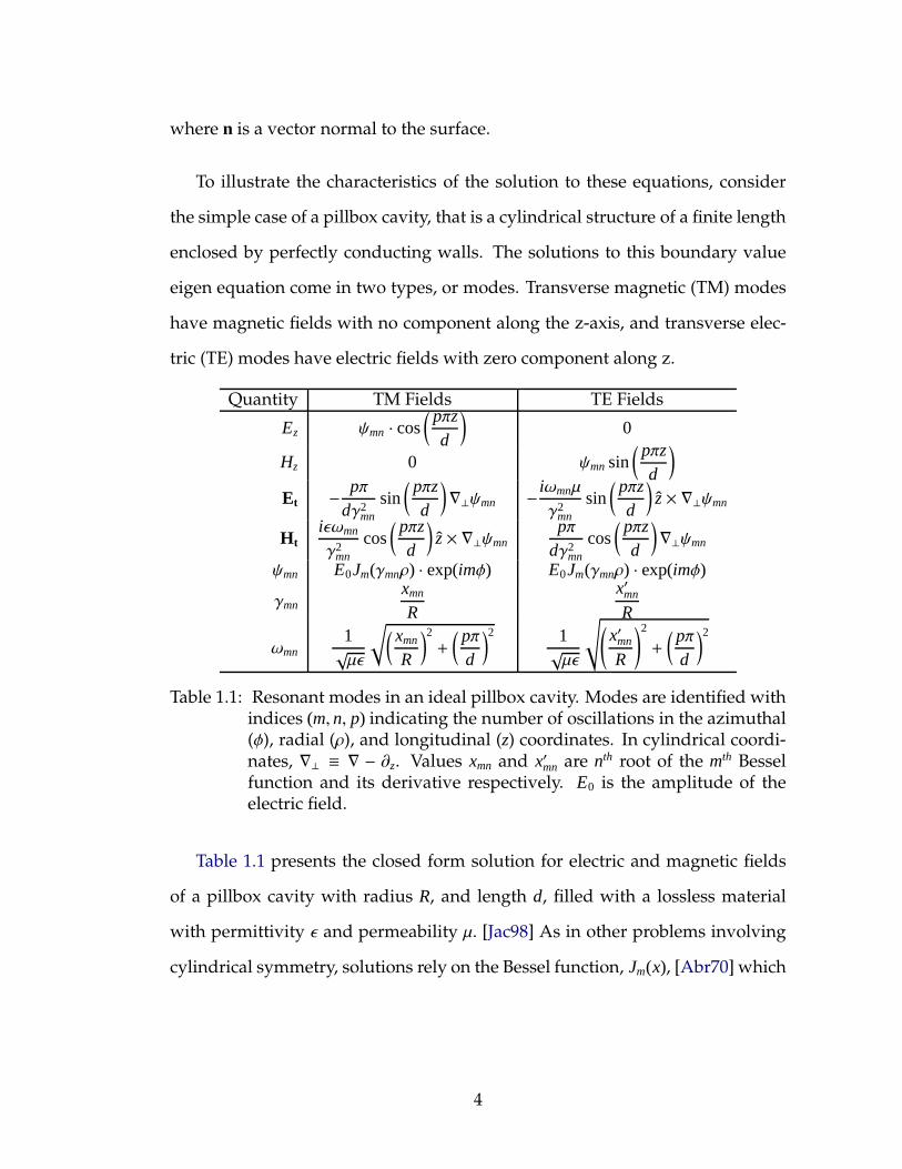
Quantity TM Fields TE Fields
Ez ψmn · cos( pπz
d
)
0
Hz 0 ψmn sin( pπz
d
)
Et − pπdγ2
mn
sin( pπz
d
)
∇⊥ψmn − iωmnµ
γ2mn
sin( pπz
d
)
z × ∇⊥ψmn
Htiǫωmn
γ2mn
cos( pπz
d
)
z × ∇⊥ψmnpπ
dγ2mn
cos( pπz
d
)
∇⊥ψmn
ψmn E0Jm(γmnρ) · exp(imφ) E0Jm(γmnρ) · exp(imφ)
γmnxmn
R
x′mn
R
ωmn1√µǫ
√( xmn
R
)2
+
( pπd
)2 1√µǫ
√(
x′mn
R
)2
+
( pπd
)2
Table 1.1: Resonant modes in an ideal pillbox cavity. Modes are identified withindices (m, n, p) indicating the number of oscillations in the azimuthal(φ), radial (ρ), and longitudinal (z) coordinates. In cylindrical coordi-nates, ∇⊥ ≡ ∇ − ∂z. Values xmn and x′mn are nth root of the mth Besselfunction and its derivative respectively. E0 is the amplitude of theelectric field.
Table 1.1 presents the closed form solution for electric and magnetic fields
of a pillbox cavity with radius R, and length d, filled with a lossless material
with permittivity ǫ and permeability µ. [Jac98] As in other problems involving
cylindrical symmetry, solutions rely on the Bessel function, Jm(x), [Abr70] which
4
can be defined by the series
Jm(x) =∞∑
α=0
(−1)α
α!Γ(α + m + 1)
( x2
)2α+m
. (1.6)
The electric and magnetic vector fields for the mode with the lowest reso-
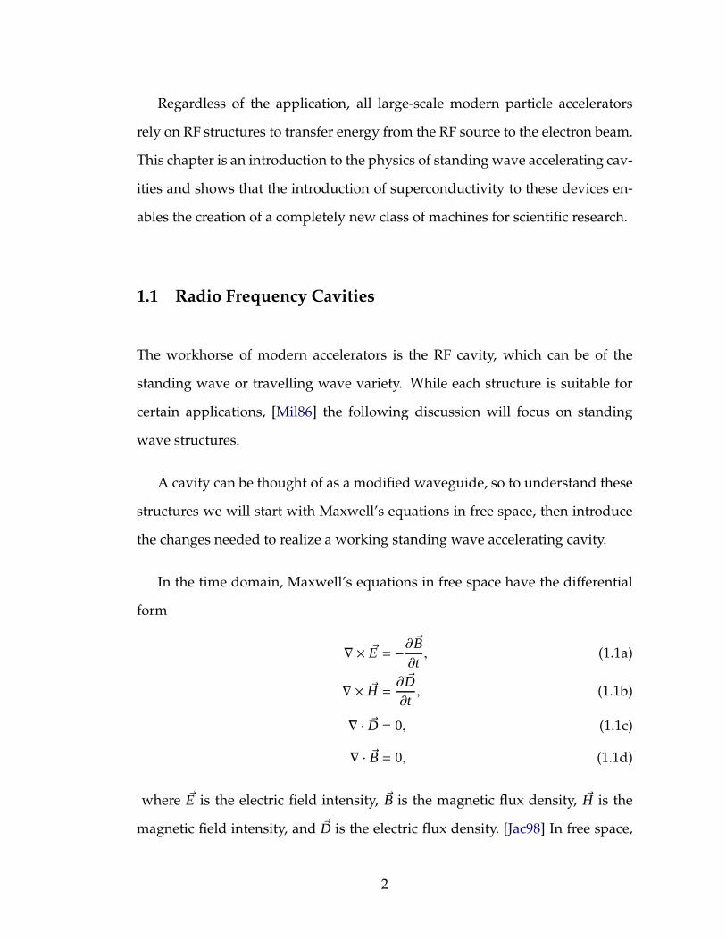
nant frequency, called the fundamental mode, in a pillbox structure with beam
tubes are presented in Figure 1.1. The equations given in Table 1.1 for an ideal
pillbox cavity do not exactly describe the field, since the beam tubes introduce a
small perturbation. Nevertheless, in this structure, and other more complicated
geometries, the concepts of TE and TM modes provide a good approximation
to the actual fields in the cavity.
Figure 1.1: Electric and magnetic fields for the TM010 mode of a pillbox cavitywith beam tubes over time. Field patterns at phases 180, 225, 270,and 315 are the same as above with the vector direction reversed.
The TM class of modes have an electric field component pointing along the z-
axis, and so, by adding an aperture to the front and end plate, a charged particle
beam passing through the structure can be accelerated by transferring energy
from the cavity to the beam. For this mode, a relativistic (β ≡ v/c = 1) charged
5
particle traveling along the cavity’s beam axis will pass through an effective
potential difference, V , given by
V =∫
E(x = 0, y = 0, z) exp[
i(ωz/c + φ)] · dz, (1.7)
where φ is the phase of the electric field at the time the particle enters the cavity.
The real part of this value gives the accelerating voltage, Vacc ≡ ℜ[V]. The ac-
celerating electric field gradient, Eacc, calculates the energy gain for a structure
with active accelerating length, L, according to
Eacc ≡Vacc
L, (1.8)
and can be maximized by proper choice of φ.
The mathematical formulation of standing wave solutions assumes the cav-
ity’s material is made of perfectly conducting material. Realistic structures have
finite conductivity, leading to an important figure of merit characterizing the
energy losses in the walls of a structure. The quality factor, Q0, is defined in
terms of the energy stored in a cavity, U, and the power dissipated in the cavity
walls, Pdiss according to
Q0 ≡ωUPdiss
, (1.9)
and has the physical interpretation that the energy stored in a cavity will de-
crease by a factor of 1/e with a time constant of Q0/ω. The energy stored in a
structure can be computed via
U =1
2µ0
$
Ω
|B(x, y, z)|2 dΩ =12ǫ0
$
Ω
|E(x, y, z)|2 dΩ (1.10)
where Ω is the volume of the cavity. [PKH98]
Modes of accelerating structures also have impedances analogous to those
encountered in circuit theory. One of the most common figures of merit for
6
monopole modes of the form TM0mp, R/Q, is defined as
RQ=|V |22ωU
, (1.11)
and physically couples the energy stored in the cavity with the effective poten-
tial difference a particle sees as it passes through the structure. [PKH98] The
factor of two is a convention used in the circuit theory analysis, though other
authors may use different definitions.
The final figure of merit is the geometry factor, G, which is a parameter cou-
pling the quality factor of a structure with its surface resistance, Rs. Because the
power dissipated in the cavity walls in Equation 1.9 can be written as
Pdiss =1
2µ20
Rs
"
A|B|2 dA, (1.12)
where A is the surface area of the cavity. Using Equation 1.10, one can write
Q0 =ωµ0
Rs·
#
Ω|B|2 dΩ
!
A|B|2 dA
. (1.13)
The geometry factor is then defined as
G ≡ Rs · Q0 = ωµ0 ·#
Ω|B|2 dΩ
!
A|B|2 dA
, (1.14)
which is only dependent on the shape of the cavity, independent of material
properties.
1.1.1 Non-fundamental mode resonances
Higher-order modes
A given accelerating structure can support an infinite number of eigen modes,
depending on possible values of m, n, and p. As the eigenvalues (frequencies)
7
of these modes are larger than the fundamental mode, they are referred to as
higher-order modes (HOMs). These modes may cause unwanted phenomena,
such as beam instability or emittance growth, in an accelerating structure, so
they should be understood thoroughly.
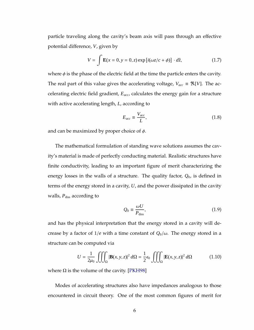
Figure 1.2 presents electric field maps for TM higher-order modes at the cen-
ter of a pillbox cavity. Modes are often referred to as monopole (m = 0), dipole
(m = 1), quadrupole (m = 2), sextupole (m = 3), or octupole (m = 4), depending
on their number of azimuthal variations; this nomenclature is frequently used
in this thesis.
Figure 1.2: Electric field component Ez at the center of a pillbox cavity for TMhigher-order modes for various values of m and n.
For modes having a non-zero number of azimuthal variations, Ez = 0 along
the beam axis. This means that Equation 1.7 is identically zero, so the impedance
of the mode via Equation 1.11 also vanishes. To remedy this situation, a trans-
8

verse voltage, V⊥, is defined for modes with m > 0 a distance r0 parallel to the
beam axis.
To derive V⊥, it is convenient to consider the modes excited by a relativistic
particle (β = 1) travelling parallel to the beam axis, but offset a distance r0 in the
direction of the HOM’s polarization axis, chosen to be in the x-direction. The
beam will couple to the z-component of the electric field. The voltage induced
by the longitudinal field scales (for small values) with radius, r, as
V(r) =
(
rr0
)m
· V(r0), (1.15)
where V(r0) is defined as in Equation 1.7, substituting x = r0, and the scaling
arises from the leading term of the series in Equation 1.6. [Sch11]
The particles are deflected by the multipole field, receiving a transverse kick,
∆p⊥, given by the Panofsky-Wenzel theorem, [PW56]
∆p⊥ = iqω
dVdr. (1.16)
Carrying out the differentiation connects the transverse and longitudinal volt-
age via
V(r)⊥ =c∆p⊥
q= i
cωr0·(
rr0
)m−1
V(r0), (1.17)
V(r0)⊥ = i
(
cωr0
) ∫
Ez(r0, z) exp(
iωzc
)
dz, (1.18)
whereω is the angular frequency of the mode, and the second equation uses r →
r0. Analogous to the longitudinal R/Q defined in Equation 1.11, the transverse
value, (R/Q)′⊥ is simply(
RQ
)′
⊥≡ |V⊥|
2
ωU, (1.19)
which is valid for all multipole modes, and used in 3D electro-magnetic simu-
lation codes such as ACE3P. [LLNK09] Note (R/Q)′⊥ has dimension Ω.
9

A 2.5D electromagnetic code1 CLANS2 [MY99] uses a slightly different defi-
nition of transverse impedance. In CLANS2,
(
RQ
)
⊥≡ |V(r0)|2
2ωUr2m0
, (1.20)
and has units of Ω/cm2m. The benefit of this definition is that (R/Q)⊥ is indepen-
dent of offset for small values of r0. This quantity appears unprimed, because it
is the standard definition used in most of this work.
Mode splitting in multi-cell structures
In addition to HOMs obtained from azimuthal, longitudinal, or radial varia-
tions, the formation of an accelerating structure composed of several resonators
(e.g. several pillbox cavities, each of which is a cell, connected by coupling
holes or irises) also introduces additional modes, due to the cell-to-cell interac-
tion. This can be modelled in terms of oscillators coupled with springs, or via
a circuit model, as illustrated in Figure 1.3. A structure comprised of N cells
will have N modes in the TM010 passband. [Lie01] The eigenfrequencies of the
ath modes in a given passband have the form
ωa = ω0
√
1+ 2kc
[
1− cos(aπ
N
)]
, (1.21)
which depend on the cell-to-cell coupling factor, kc, assumed constant between
cells in the above equations. [Lie01] Figure 1.4 presents the relative field ampli-
tude for the fundamental passband of a 7-cell cavity.
In addition to mode splitting between cells in a structure, it is also possi-
ble to introduce additional modes by the coupling of multicell structures with
1CLANS2 models 2D structures, but accounts for azimuthal variations of multipole modesfor cylindrically symmetric structures, giving it the extra 1/2 dimension.
10

Figure 1.3: Top: Circuit model of coupled cavities modeled as RLC circuitsdriven by a current source with capacitive coupling. [Lie01]. Bot-tom: Coupled pendula model illustrating the different coupling ofcavities in at the end of a cavity string with those coupled to cavitieson both sides.
one another. [Lie01] In general this coupling is extremely weak for the funda-
mental mode because beam tubes are chosen so that the fundamental mode is
strongly attenuated outside of a given resonant structure. Higher-order modes
may propagate out of a given cavity and couple with those of other cavities.
At this point, the basic theory of electromagnetic fields in resonant cavities
has been introduced. Next, attention is turned to the benefits of coupling this
technology with superconducting science.
1.2 Introduction to Superconductivity
Superconductivity is a phenomena that was first discovered by Kamerlingh
Onnes in 1911, wherein he measured the temperature dependent resistance of
a column of mercury at very low temperatures. He found that below 4.2 K,
11

1 2 3 4 5 6 71
2
3
4
5
6
7
Fie
lddistr
ibution
inth
enπ/7
mode
Cell Number
Figure 1.4: Amplitude distribution of modes 7-cell cavity’s fundamental pass-band. The 7π/7 mode has equal amplitude in all cells, and is used asthe fundamental accelerating mode.
the resistance of the mercury dropped sharply from ≈0.1 Ω to less than 1 µΩ
of resistance (a value too small to measure with his instruments). [Onn11] Fig-
ure 1.5 shows the first measurement of a superconducting sample, a feat for
which Onnes received the Nobel Prize in Physics, just two years later. [Nob13a]
Subsequent measurements of the resistivity of superconductors to direct cur-
rent showed that the ratio of the resistivity in the superconducting state to the
normal conducting state was less than 2 × 10⁻¹⁶. [Bro61] Thus, in DC, a super-
conductor can be considered a perfect conductor, and the physics of perfect con-
ductors can shed insight into the workings of superconductors without delving
into the full microscopic theory; more about the theory will be presented in
chapter 2. The arguments below follow the presentation in Padamsee’s ”RF Su-
perconductivity for Accelerators.” [PKH98]
12
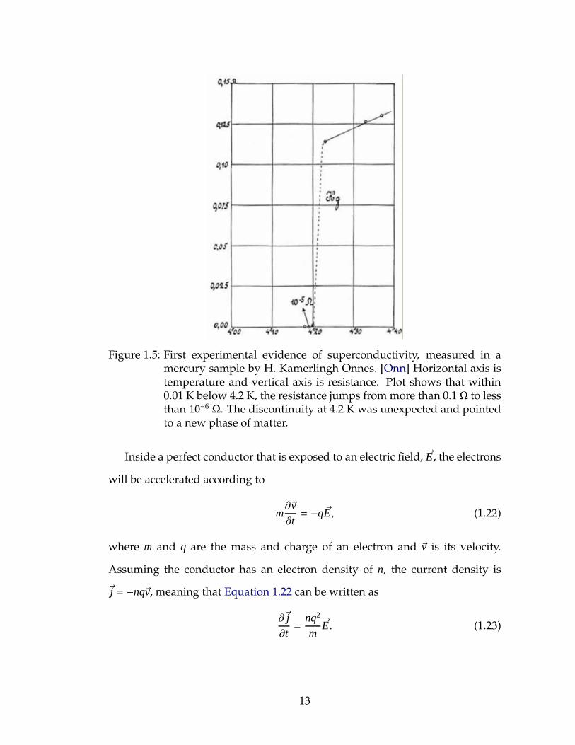
Figure 1.5: First experimental evidence of superconductivity, measured in amercury sample by H. Kamerlingh Onnes. [Onn] Horizontal axis istemperature and vertical axis is resistance. Plot shows that within0.01 K below 4.2 K, the resistance jumps from more than 0.1 Ω to lessthan 10−6
Ω. The discontinuity at 4.2 K was unexpected and pointedto a new phase of matter.
Inside a perfect conductor that is exposed to an electric field, ~E, the electrons
will be accelerated according to
m∂~v∂t= −q~E, (1.22)
where m and q are the mass and charge of an electron and ~v is its velocity.
Assuming the conductor has an electron density of n, the current density is
~j = −nq~v, meaning that Equation 1.22 can be written as
∂~j∂t=
nq2
m~E. (1.23)
13
Using the result of Equation 1.23 in Equation 1.1a one arrives at the result
∂
∂t
∇ × ~j +nq2
m~B
= 0. (1.24)
For static fields, there is no displacement current and ∇×~B = µ0~j, so applying
this relation to Equation 1.24 yields
∇2 − 1
λ2L
~B = 0, (1.25)
where λL is the London penetration depth
λL ≡√
mµ0nq2
, (1.26)
which gives the distance into the perfect conductor at which the magnetic flux
density drops by a factor of 1/e, when exposed to an external uniform magnetic
field.
Superconductors exhibit one important difference compared with perfect
conductors: the ability to expel magnetic flux from the material bulk, when
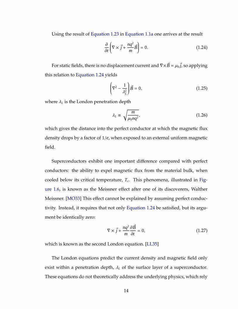
cooled below its critical temperature, Tc. This phenomena, illustrated in Fig-
ure 1.6, is known as the Meissner effect after one of its discoverers, Walther
Meissner. [MO33] This effect cannot be explained by assuming perfect conduc-
tivity. Instead, it requires that not only Equation 1.24 be satisfied, but its argu-
ment be identically zero:
∇ × ~j + nq2
m∂~B∂t= 0, (1.27)
which is known as the second London equation. [LL35]
The London equations predict the current density and magnetic field only
exist within a penetration depth, λL of the surface layer of a superconductor.
These equations do not theoretically address the underlying physics, which rely
14
Figure 1.6: Illustration of the Meissner effect. At left, a superconductor at a tem-perature above Tc is positioned in a uniform magnetic field. Shownat right is the same setup after cooling the material below Tc, whichcauses flux to be expelled from the bulk of the superconductor.
on a microscopic explanation, and as such do not explain such phenomena as
flux pinning, but do adequately provide a broad explanation of empirical re-
sults.
Superconductivity arises from the pairing of electrons due to a weak attrac-
tive potential caused by lattice distortions as electrons pass through a mate-
rial. [BCS57] This changes the density of states present in a normal conductor to
one in which an energy gap, Eg, appears between states with paired electrons
and vacant states. As such, it costs energy to break up electron pairs, known as
Cooper pairs, and the superconducting state is energetically favorable.
It is important to note that the pairing between electrons is not a tight one,
as is the pairing between an electron and an atomic nucleus. Cooper pairs
have correlated spin and momenta as between particles having (~p, ↑) and (−~p, ↓).
[PKH98] The rough distance of coherence between the pairs can be calculated.
The condensing electrons are those with momenta sufficient to place their
15
energy near the Fermi energy kBTc. This allows one to write
kBTc = δ
p2
2m
=pmδp, (1.28)
δp =kBTc
vF, (1.29)
where the Fermi velocity vF ≡ p/m has been introduced. The minimal spatial
extent of the pair, ξ, is limited by the Heisenberg uncertainty principle, ξ · δp = ~
to yield
ξ =~vF
kBTc. (1.30)
While the actual definition of coherence length varies based on which theoretical
frame work is being used (see Appendix A for a full discussion), Equation 1.30
provides a qualitative description of the correlation length between paired elec-
trons.
With the qualitative properties of superconductors introduced, the interface
between accelerator physics and superconductivity will be explored.
1.2.1 Superconductivity applied to accelerating structures
Modern accelerating structures rely on oscillating RF fields. The discussion in
the previous section holds true for static fields, but modifications are necessary
to treat the RF case. The first needed modification is to note that in an RF field,
the conductivity of Cooper pairs is not infinite, due to their inertial mass.
One of the most significant benefits of RF superconducting structures is their
extremely small, yet finite, surface resistance. The surface impedance can be
calculated by assuming that the conductivity is due to normal conducting elec-
16
trons, σn, and superconducting electrons, σs. The surface impedance, Zs, due to
an RF oscillation of frequency ω is
Zs = Rs + iXs =
√
iωµ0
σn − iσs. (1.31)
where Rs is the resistance of the structure and Xs is the reactance. [PKH98] As-
suming the conductivity of the superconducting electrons is much greater than
those of the normal conducting electrons, the real and imaginary parts of the
impedance becomes
Rs =12σnω
2µ20λ
3L, (1.32)
Xs = ωµ0λL. (1.33)
It is important to note that λL is temperature dependent, which can change Rs by
orders of magnitude from temperatures near Tc to the low temperatures used in
SRF operation. In general Rs ≫ Xs for superconductors. [PKH98] The actual val-
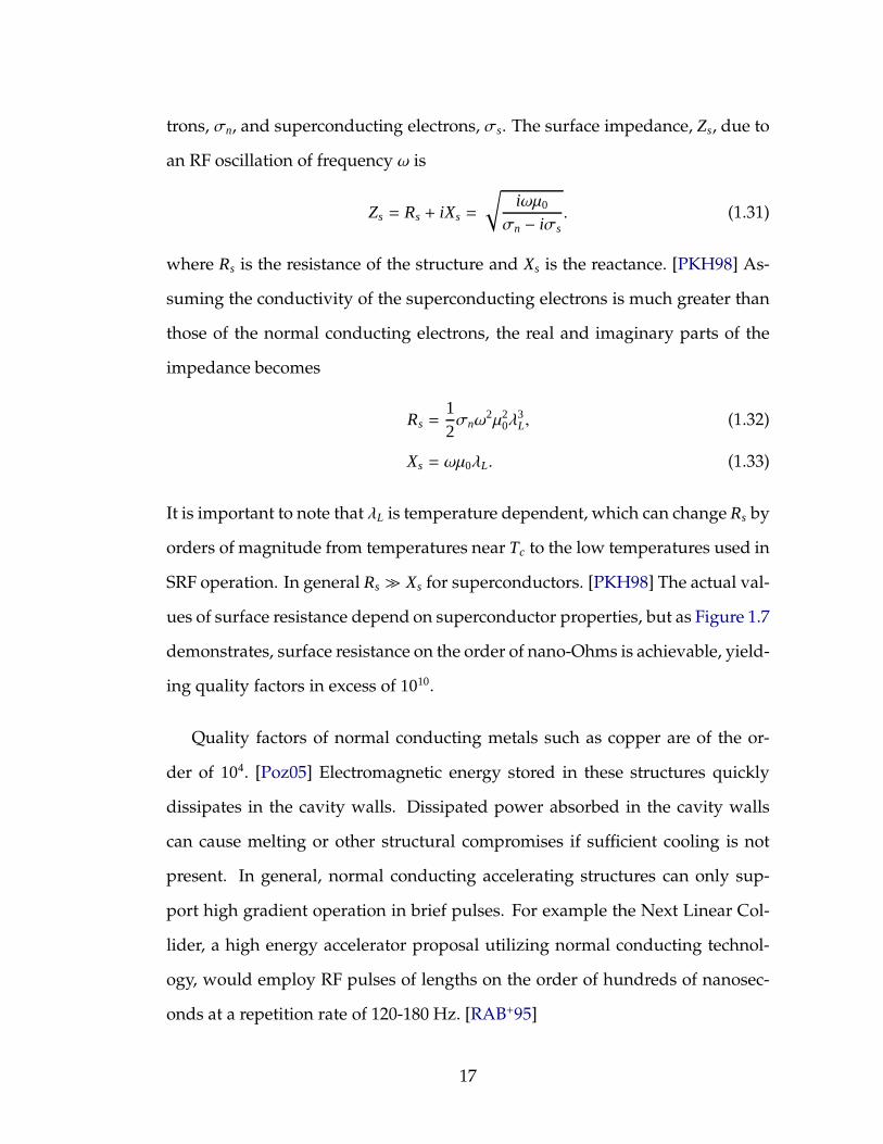
ues of surface resistance depend on superconductor properties, but as Figure 1.7
demonstrates, surface resistance on the order of nano-Ohms is achievable, yield-
ing quality factors in excess of 1010.
Quality factors of normal conducting metals such as copper are of the or-
der of 104. [Poz05] Electromagnetic energy stored in these structures quickly
dissipates in the cavity walls. Dissipated power absorbed in the cavity walls
can cause melting or other structural compromises if sufficient cooling is not
present. In general, normal conducting accelerating structures can only sup-
port high gradient operation in brief pulses. For example the Next Linear Col-
lider, a high energy accelerator proposal utilizing normal conducting technol-
ogy, would employ RF pulses of lengths on the order of hundreds of nanosec-
onds at a repetition rate of 120-180 Hz. [RAB+95]
17

T/Tc
Rs
[Ω]
0 0.2 0.4 0.6 0.8 110
−9
10−8
10−7
10−6
10−5
10−4
10−3
Typical Nb Surface ResistanceTypical Operating Temperature
Figure 1.7: Typical RF surface resistance of superconducting niobium (assum-ing a residual resistance of 3 nΩ) at 1300 MHz calculated from BCStheory with SRIMP. [Hal70b] The blue region shows the region oftemperatures usually chosen for superconducting accelerators.
In contrast, superconducting RF structures, with their extremely small sur-
face resistances, regularly achieve quality factors in excess of 1010 at high gradi-
ents. The power loss in the walls is reduced by orders of magnitude, allowing
continuous wave operation of accelerators at high gradients.
A brief back of the envelope calculation demonstrates the benefits of super-
conductivity in accelerators operating in continuous wave mode: A multicell
cavity operating at an accelerating gradient of 20 MV/m with a frequency of
1300 MHz stores just under 20 J of energy in the structure. A copper cavity at
room temperature, having Q0 = 104 would dissipate 15 MW of power in the
cavity walls, leading to power densities that could not be removed by a cooling
system. The same structure, composed of superconducting niobium, operating
at 1.8 K, would only dissipate approximately 15 W of power. Even including
18
the inefficiency of power extraction at cryogenic temperatures, which requires
about 1000 W of wall power for each Watt removed at 1.8 K, superconducting RF
structures provide huge energy savings, and the realization of scientific devices
that are infeasible without the technology.
1.2.2 RF Characterization of Superconducting Cavities
One of the primary benefits of utilizing superconductors in accelerating struc-
tures is the extremely high quality factors. A technique is needed to accurately
measure this figure of merit for resonant cavities. The theory behind RF mea-
surements of superconducting resonators is well understood, so below the basic
features are highlighted, following [PKH98].
Supposing energy, U is stored in a cavity with resonant angular frequency,
ω, losses will cause the energy to decay as a function of time, t, according to
dUdt= − U
τL(t). (1.34)
In the above equation, the time constant, τL, for dissipation of energy in the
cavity is defined as
τL(t) =ω
QL(t), (1.35)
and can be measured with a power meter. The loaded quality factor of the struc-
ture, QL, takes into account the overall quality factor due to multiple sources of
losses, such as the cavity wall (Q0) and the power coupled out via RF input
coupler (Qe), and field probe (Qt). These quantities are related as
1QL=
1Q0+
1Qe+
1Qt. (1.36)
19

By design, the losses to the field probe are small and can usually be neglected.
The quantity of interest is Q0, since it is an intrinsic property of the resonator
independent of coupling scheme. For this reason, Q0 is often called the intrinsic
quality factor.
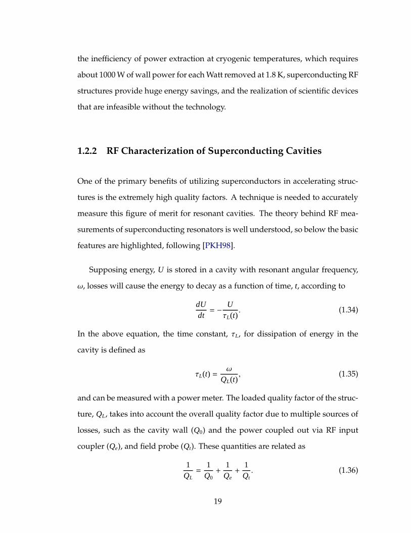
The coupling between the RF input coupler and the cavity is characterized
through a coupling constant β = Q0/Qe. This constant can be measured by turn-
ing off input power to the cavity and measuring power levels reflected from the
cavity coupler at several points in time to calculate
βe =1
2√
Pi
Pe− 1
, (1.37)
βi =
1±√
Pr
Pi
1∓√
PrPi
, (1.38)
whose average yields β. In Equation 1.38, the upper sign is used when β > 1
and the lower sign when β < 1. [PKH98] The definitions of Pi, Pe, and Pr come
from the reflected power trace, as illustrated in Figure 1.8.
Figure 1.8: Reflected power signal as a function of time for an under-coupledcavity. Geometric symbols mark the points on the trace giving val-ues used in Equation 1.37 and Equation 1.38. The box labelled ”RFPower On” marks the time period in which the cavity is driven onresonance with constant drive power.
20
The intrinsic quality factor is given by
Q0 = ω · τL · (1+ β). (1.39)
Software was developed to automate the data taking process, [GVL12] greatly
simplifying the characterization of superconducting resonators.
The accelerating gradient can be determined by measuring the power cou-
pled out of the cavity with a field probe, Pt, with very weak coupling Qt, to a
mode with shunt impedance (R/Q). Recalling the relation P = V2/R, the voltage
in the structure is given by
V =
√
2 · Pt ·(
RQ
)
· Qt, (1.40)
where the factor of 2 arises from use of the circuit definition of (R/Q). For a
cavity driven at a constant power, P f , from an input coupler with Qext coupling
to the mode, the voltage in the cavity is given by
V =2 · βe
1+ βe·√
2 · P f ·(
RQ
)
· Qext . (1.41)
The accelerating gradient is obtained by dividing by the appropriate length, as
discussed in Equation 1.8.
It is also possible to relate the peak surface electric or magnetic field (which
usually occur at different locations) and the stored energy in the structure, U,
via electromagnetic constants ke and km obtained from field solving codes. They
are related via
Epk = ke ·√
U, (1.42)
Bpk = km ·√
U. (1.43)
21

1.3 Superconducting Properties of Niobium
To date, niobium is the only superconducting material that has been utilized in
the accelerating structures of large-scale projects. There are many reasons for
this, including its (relatively) high critical temperature, its mechanical proper-
ties including ductility and high thermal conductivity, and the S-wave nature
of its superconductivity. The benefits of each of these properties will each be
discussed in turn.
The first benefit of niobium is that of all pure substances, it has the high-
est critical temperature, as shown in Table 1.2. Generally speaking, for type-I
superconductors, the maximum magnetic field a superconductor can support
in the Meissner state is proportional to the critical temperature. Specifically, a
superconductor with critical temperature Tc, operating at a temperature T , can
support magnetic surface fields that increase as T/Tc → 0. This has direct conse-
quences for accelerators in that materials capable of supporting higher fields
require less real estate to operate at high energies. An additional benefit of
choosing to use a superconductor with a higher Tc is the fact that cryogenic
systems become more technologically challenging at low temperatures, making
installation and operation costs prohibitively expensive for large installations.
In addition to the benefits of its high critical temperature, niobium has sev-
eral properties that make it suitable for forming into accelerating structures. It is
ductile, and can be rolled, pressed or hydroformed into cavity shapes. Further-
more, it can be produced in high purity ingots, with low resistivity at cryogenic
temperatures. A parameter characterizing the purity of the niobium in terms of
the ratio of its room temperature and cryogenic resistivity, the residual resistiv-
22
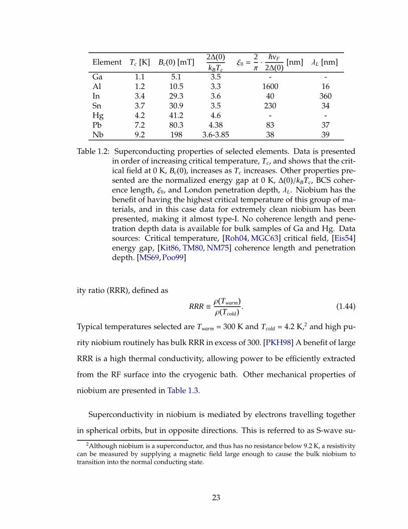
Element Tc [K] Bc(0) [mT]2∆(0)kBTc
ξ0 =2π· ~vF
2∆(0)[nm] λL [nm]
Ga 1.1 5.1 3.5 - -Al 1.2 10.5 3.3 1600 16In 3.4 29.3 3.6 40 360Sn 3.7 30.9 3.5 230 34Hg 4.2 41.2 4.6 - -Pb 7.2 80.3 4.38 83 37Nb 9.2 198 3.6-3.85 38 39
Table 1.2: Superconducting properties of selected elements. Data is presentedin order of increasing critical temperature, Tc, and shows that the crit-ical field at 0 K, Bc(0), increases as Tc increases. Other properties pre-sented are the normalized energy gap at 0 K, ∆(0)/kBTc, BCS coher-ence length, ξ0, and London penetration depth, λL. Niobium has thebenefit of having the highest critical temperature of this group of ma-terials, and in this case data for extremely clean niobium has beenpresented, making it almost type-I. No coherence length and pene-tration depth data is available for bulk samples of Ga and Hg. Datasources: Critical temperature, [Roh04, MGC63] critical field, [Eis54]energy gap, [Kit86, TM80, NM75] coherence length and penetrationdepth. [MS69, Poo99]
ity ratio (RRR), defined as
RRR ≡ ρ(Twarm)ρ(Tcold)
. (1.44)
Typical temperatures selected are Twarm = 300 K and Tcold = 4.2 K,2 and high pu-
rity niobium routinely has bulk RRR in excess of 300. [PKH98] A benefit of large
RRR is a high thermal conductivity, allowing power to be efficiently extracted
from the RF surface into the cryogenic bath. Other mechanical properties of
niobium are presented in Table 1.3.
Superconductivity in niobium is mediated by electrons travelling together
in spherical orbits, but in opposite directions. This is referred to as S-wave su-
2Although niobium is a superconductor, and thus has no resistance below 9.2 K, a resistivitycan be measured by supplying a magnetic field large enough to cause the bulk niobium totransition into the normal conducting state.
23
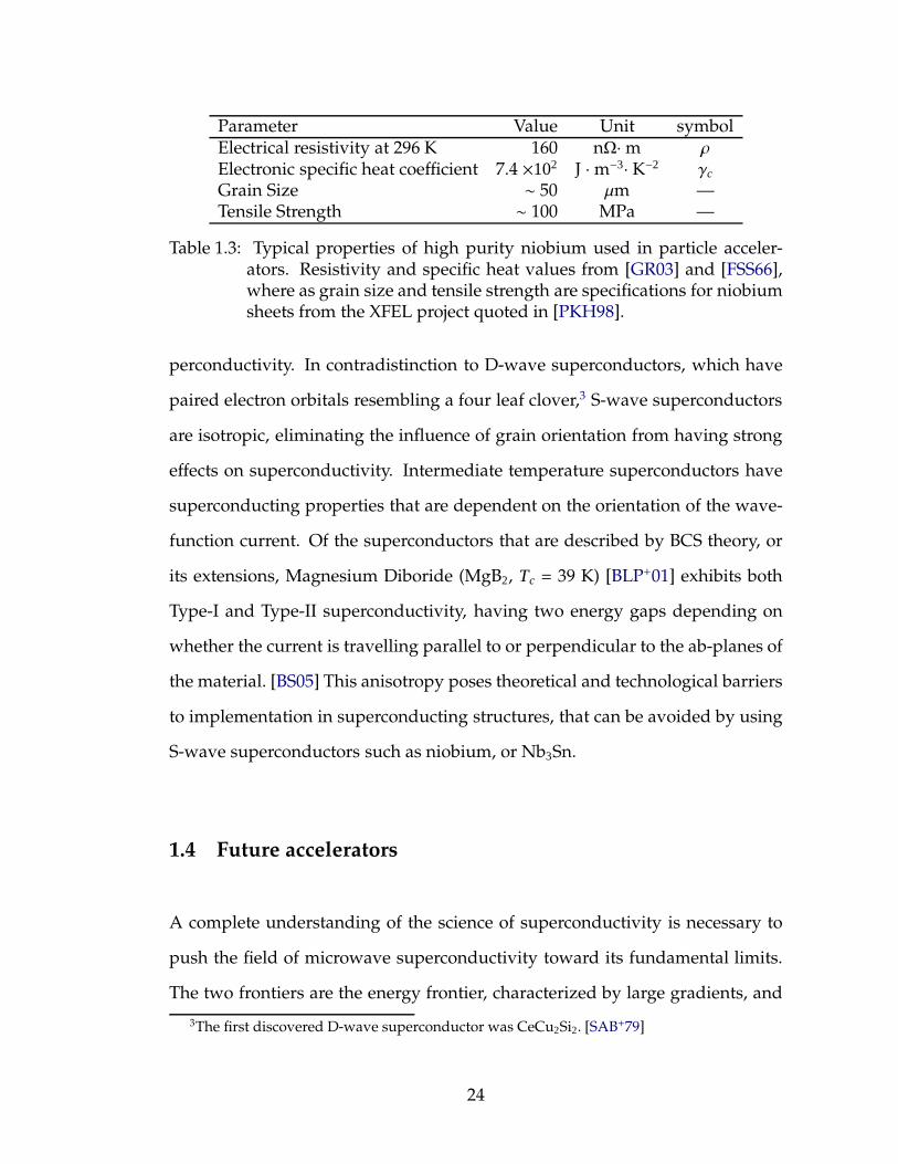
Parameter Value Unit symbolElectrical resistivity at 296 K 160 nΩ·m ρ
Electronic specific heat coefficient 7.4 ×10² J ·m−3· K−2 γc
Grain Size ∼ 50 µm —Tensile Strength ∼ 100 MPa —
Table 1.3: Typical properties of high purity niobium used in particle acceler-ators. Resistivity and specific heat values from [GR03] and [FSS66],where as grain size and tensile strength are specifications for niobiumsheets from the XFEL project quoted in [PKH98].
perconductivity. In contradistinction to D-wave superconductors, which have
paired electron orbitals resembling a four leaf clover,3 S-wave superconductors
are isotropic, eliminating the influence of grain orientation from having strong
effects on superconductivity. Intermediate temperature superconductors have
superconducting properties that are dependent on the orientation of the wave-
function current. Of the superconductors that are described by BCS theory, or
its extensions, Magnesium Diboride (MgB2, Tc = 39 K) [BLP+01] exhibits both
Type-I and Type-II superconductivity, having two energy gaps depending on
whether the current is travelling parallel to or perpendicular to the ab-planes of
the material. [BS05] This anisotropy poses theoretical and technological barriers
to implementation in superconducting structures, that can be avoided by using
S-wave superconductors such as niobium, or Nb3Sn.
1.4 Future accelerators
A complete understanding of the science of superconductivity is necessary to
push the field of microwave superconductivity toward its fundamental limits.
The two frontiers are the energy frontier, characterized by large gradients, and
3The first discovered D-wave superconductor was CeCu2Si2. [SAB+79]
24
the power frontier, characterized by extremely high quality factors. It is the
purpose of this thesis to elucidate the connection between these two frontiers
for niobium material.
1.4.1 Pulsed High Gradient Accelerators
In 1964 a group of physicists postulated the existence of an undiscovered par-
ticle as the mechanism behind inertial mass of matter. [EB64, Hig64, GHK64] In
the intervening 49 years, a collaboration of more than 2,000 scientists working
at CERN designed the world’s largest particle accelerator to detect this massive
particle, a key discovery leading to the key theorists receiving the 2013 Nobel
Prize in Physics. [Nob13b]
Though the Higgs boson has been detected, a great many questions about
the underlying fabric of the universe remain: Are there undiscovered principles
of nature? What is dark matter and dark energy? At high energies, do all forces
become one? Does the universe exhibit supersymmetry? Hints at solutions to
these problems are being provided by the Large Hadron Collider, but further
illumination requires precision measurements possible with higher energy ma-
chines such as the International Linear Collider. [Pan05]
To achieve a center-of-mass energy of 500 GeV, the 30.5 km long accelerator
sections consisting of niobium superconducting cavities must operate in pulsed
mode at average gradients of 31.5 MV/m, corresponding to surface magnetic
fields of about 135 mT. [The13a] Can the gradient be increased further to push to
even higher energy regimes? What is the intrinsic limitation to operating these
niobium structures at very high gradients? These questions are further explored
25
in chapter 2 by exploring a fundamental limitation to surface magnetic fields on
superconducting niobium, the magnetic superheating field.
1.4.2 High Efficiency CW Accelerators
In recent years, many applications of CW accelerators have been proposed.
Science projects such as free-electron lasers (LCLS-II at SLAC [BBD+12]), pro-
ton based CW linac machines (Project-X at Fermilab [OSB+12]) and accelera-
tor driven systems (ADS being investigated at multiple locations worldwide
[Age99]) all rely on SRF technology pushing the efficient limit. These machines
do not require extreme gradients to minimize total costs, as illustrated by cost
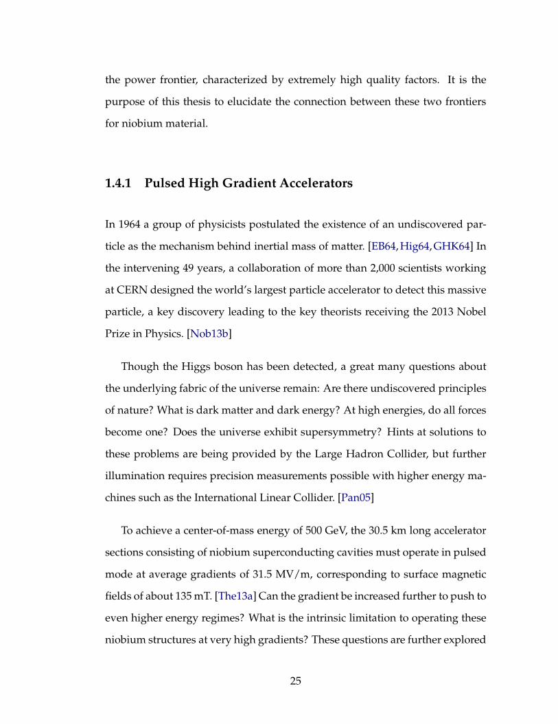
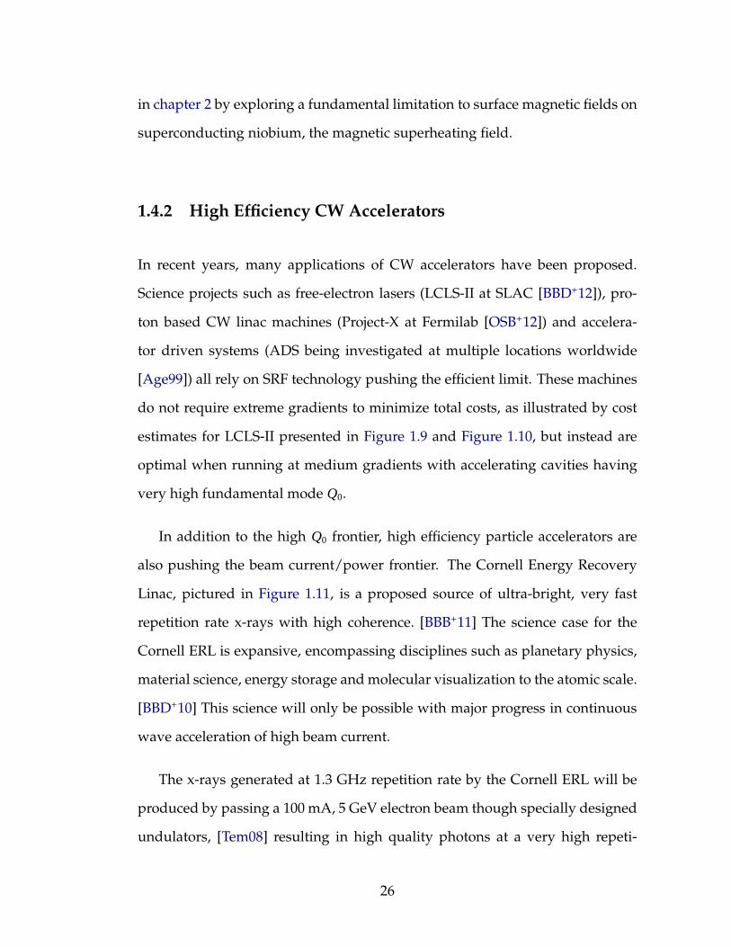
estimates for LCLS-II presented in Figure 1.9 and Figure 1.10, but instead are
optimal when running at medium gradients with accelerating cavities having
very high fundamental mode Q0.
In addition to the high Q0 frontier, high efficiency particle accelerators are
also pushing the beam current/power frontier. The Cornell Energy Recovery
Linac, pictured in Figure 1.11, is a proposed source of ultra-bright, very fast
repetition rate x-rays with high coherence. [BBB+11] The science case for the
Cornell ERL is expansive, encompassing disciplines such as planetary physics,
material science, energy storage and molecular visualization to the atomic scale.
[BBD+10] This science will only be possible with major progress in continuous
wave acceleration of high beam current.
The x-rays generated at 1.3 GHz repetition rate by the Cornell ERL will be
produced by passing a 100 mA, 5 GeV electron beam though specially designed
undulators, [Tem08] resulting in high quality photons at a very high repeti-
26
10 15 20 2550
60
70
80
90
100
110
Eacc [MV/m]
Norm
alize
dco
st[%
]
Q0 = 1× 10¹⁰
Q0 = 2× 10¹⁰
Q0 = 4× 10¹⁰
Q0 = 6× 10¹⁰
Figure 1.9: Normalized cost vs accelerating gradient for LCLS-II, including cry-omodules, cryoplant and RF power for given SRF cavity Q0.
tion rate. The ERL will have spectral brightness orders of magnitudes higher
than other synchrotron based light sources, [BBD+10] and even yield coherent
flux similar that of FEL devices as shown in Table 1.4. Though FELs produce
very high intensity light, the less intense, but much higher repetition rate of
photons produced by the Cornell ERL allows non-destructive testing of sam-
ples and ultra-fast science via ”tickle and probe” methods [DGB+11] for inves-
tigations such as time-resolved synchrotron radiation excited optical lumines-
cence. [SR07]
The prospect of a high current ERL has spurred significant research and de-
velopment. The successful operation of the light source requires maintaining
the ultra-low emittance of the high-current beam. Reaching the Cornell ERL
specified beam current of 100 mA requires more than an order of magnitude im-
provement over the previous ERL current record [TBD+05]. This can be accom-
27
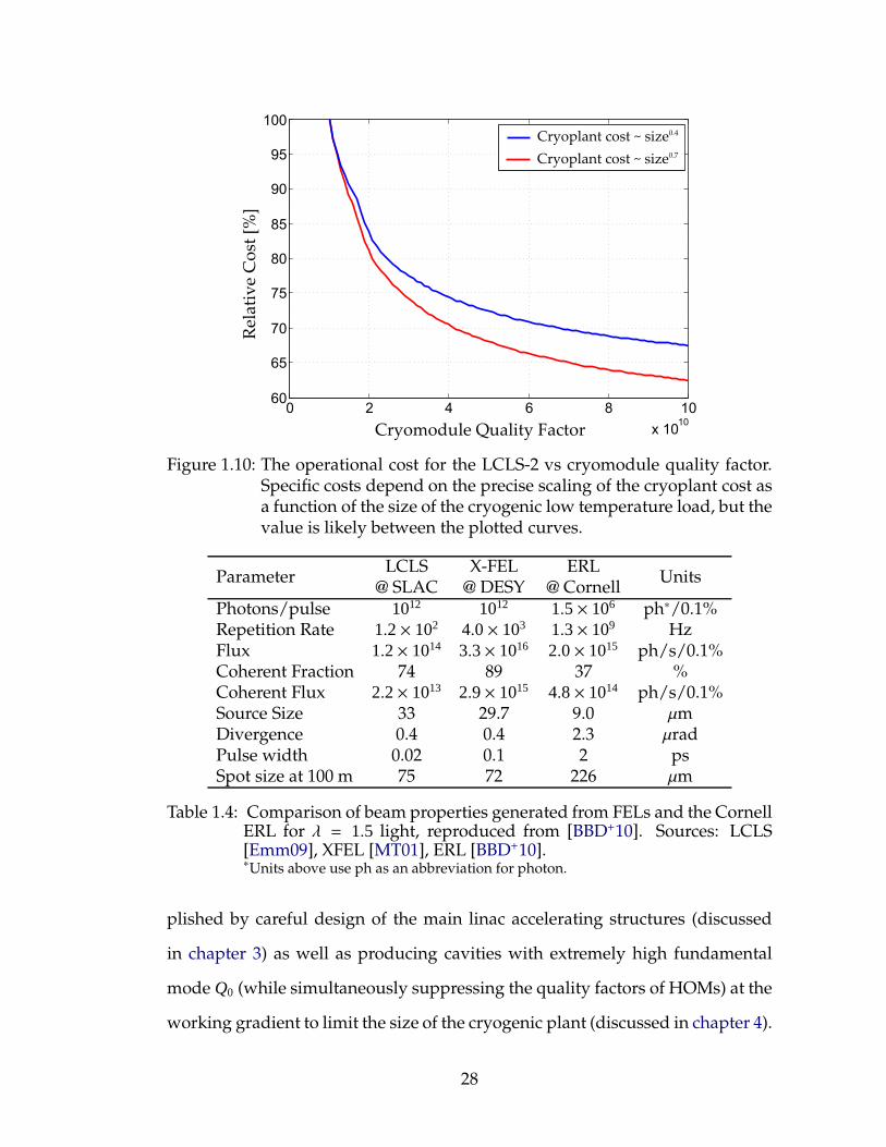
Figure 1.10: The operational cost for the LCLS-2 vs cryomodule quality factor.Specific costs depend on the precise scaling of the cryoplant cost asa function of the size of the cryogenic low temperature load, but thevalue is likely between the plotted curves.
ParameterLCLS X-FEL ERL
Units@ SLAC @ DESY @ Cornell
Photons/pulse 1012 1012 1.5× 10⁶ ph∗/0.1%Repetition Rate 1.2× 10² 4.0× 10³ 1.3× 10⁹ HzFlux 1.2× 10¹⁴ 3.3× 10¹⁶ 2.0× 10¹⁵ ph/s/0.1%Coherent Fraction 74 89 37 %Coherent Flux 2.2× 10¹³ 2.9× 10¹⁵ 4.8× 10¹⁴ ph/s/0.1%Source Size 33 29.7 9.0 µmDivergence 0.4 0.4 2.3 µradPulse width 0.02 0.1 2 psSpot size at 100 m 75 72 226 µm
Table 1.4: Comparison of beam properties generated from FELs and the CornellERL for λ = 1.5 light, reproduced from [BBD+10]. Sources: LCLS[Emm09], XFEL [MT01], ERL [BBD+10].∗Units above use ph as an abbreviation for photon.
plished by careful design of the main linac accelerating structures (discussed
in chapter 3) as well as producing cavities with extremely high fundamental
mode Q0 (while simultaneously suppressing the quality factors of HOMs) at the
working gradient to limit the size of the cryogenic plant (discussed in chapter 4).
28

Figure 1.11: An overhead view of the site layout for Cornell’s ERL. The acceler-ator uses part of the Cornell Electron Storage Ring (CESR) as a re-turn arc, and extends tunnels to allow for two accelerating sectionswhere electron beams are simultaneously accelerated and deceler-ated. [BBB+11]
Contributing to the success of the ERL main linac project in these two capacities
is a central objective of this thesis, and, as mentioned at the beginning of this
section, has applications far beyond a single project.
1.5 Summary and Organization of this Dissertation
Superconducting RF science lies at the nexus between accelerator physics and
material science, perfectly positioned to address questions related to both the
gradient frontier of high energy particle accelerator projects as well as research
challenges in developing very efficient superconducting accelerating structures.
The pages ahead address the material science of S-Wave superconductors by
investigating the superheating field of niobium (chapter 2), optimal accelerating
29
structure design for the main linac of next generation ERL light source, capable
of supporting threshold beam current well in excess of 100 mA (chapter 3), and
conclusively demonstrate that prototype tests of the Cornell ERL main linac
cavity show that extremely high quality factors are not only possible, but due
to new material insights, can be expected (chapter 4). The conclusions that can
be drawn from this work is discussed as well as highlighting opportunities for
future investigation (chapter 5).
30
CHAPTER 2
MATERIAL STUDIES: THE SUPERHEATING FIELD OF NIOBIUM
What is the maximum gradient that can be obtained for a perfect accelerat-
ing structure? This question is of central importance in designing accelerators
that push the energy frontier, and of course is material dependent. For super-
conducting structures, the theoretical answer is that the Meissner state can only
meta-stably persist up to the magnetic superheating field before undergoing a
phase transition.1 While the superheating field is understood near a material’s
critical temperature, Tc, the temperature dependence is still an open question.
This work is important because SRF accelerators utilize niobium, and op-
erate far from temperatures where rigorous results apply. This chapter inves-
tigates the temperature dependence of the superheating field of niobium, for
surface preparations commonly used in large-scale accelerators.
The chapter begins by discussing the basic critical fields of superconductors,
including the superheating field. Focusing on the superheating field, various
theories are discussed followed by a review of measurements done prior to this
work.
Next, new experimental measurements on the temperature dependence of
the superheating field of niobium are presented for two different surface treat-
ments. The presentation includes a description of the methodology used to ob-
tain the data and subsequent analysis. The chapter concludes by showing that,
for niobium, the experimental measurements of the superheating field results
1The maximum surface magnetic field in an SRF cavity is proportional to the acceleratingelectric gradient produced by the cavity, so throughout this chapter the concepts of maximummagnetic field and electric gradient are used interchangeably.
31
over a broad range of temperatures is well described by a linear dependence on
(T/Tc)2, in agreement with of Ginsburg-Landau Theory near Tc.
2.1 Introduction to the Theories of Superconductivity
As discussed in section 1.2, superconductivity is a phenomena characterized by
the ability to conduct direct current with zero attenuation. The superconducting
phase persists below critical points. For the purposes of this chapter, the critical
points of interest are external or applied magnetic fields that initiate a phase
transition out of the superconducting state at certain critical field values.
There are several approaches to understanding the behavior of supercon-
ductors near critical points. The simplest model is a phenomenological one,
based on the theory of phase transitions, put forth at the very beginning of the
1950’s by V. L. Ginsburg and L. D. Landau, which could explain the behavior of
superconductors without examining their microscopic properties. [GL50] (An
English translation appears in [Lan65])
A microscopic theory of superconductivity was not known until 1956 when
L. N. Cooper demonstrated that electrons near the Fermi surface of a material
could form an instability in the presence of an arbitrarily weak attractive po-
tential. [Coo56] The following year, J. Bardeen, L. N. Cooper and J. R. Schrief-
fer incorporated this calculation into a full framework microscopically describ-
ing the phenomena of superconductivity from the interaction between the elec-
trons and phonons in a vibrating crystal lattice, which is known as BCS the-
ory. [BCS57]
In 1959, L. P. Gor’kov demonstrated that the Ginsburg-Landau (GL) equa-
32
tions could be obtained from the microscopic considerations of BCS theory.
[Gor59] This work set the GL equations on strong theoretical footing, and has al-
lowed the model to confidently be applied to the properties of superconductors
near the critical temperature.
2.1.1 Interaction of Superconductors and Magnetic Fields
Supposing a superconductor in a constant magnetic field is cooled below its
critical temperature, then the magnetic field will be expelled from the bulk of
the superconductor, a phenomena known as the Meissner effect. [MO33] This is
accomplished by superconducting electrons establishing a magnetization can-
celling the applied field in the bulk of the material.
Due to the Meissner effect, the magnetic field in a superconductor is limited
to a small region close to the surface, characterized by a penetration depth, λL,
which is the region in which supercurrents flow. The Ginsburg-Landau coher-
ence length, ξGL is related to the spatial variation of the superconducting order
parameter.2 In addition, GL theory uses a penetration depth, λGL that is related
to λL, ξ0, and the purity of the superconductor. [OMFB79]3 The ratio of these
GL characteristic length scales yields the dimensionless Ginsburg-Landau (GL)
parameter,
κGL ≡λGL
ξGL. (2.1)
This parameter, κGL, separates superconductors into two broad categories;
2A plethora of length scales will be bandied about in the following pages. For a quick refer-ence of these lengths and their definitions, see Appendix A.
3Fortunately for pure superconductors, λL is nearly equal to λGL meaning the arguments arequalitatively correct either way.
33
those with κGL < 1/√
2 are called Type-I superconductors and those with
κGL > 1/√
2 are called Type-II superconductors.4 Though the distinction will
be dealt with more thoroughly later in this chapter, roughly speaking, Type-I
superconductors exist in either the fully superconducting state or in the nor-
mal state. Type-II superconductors can exist in a mixed state wherein normal
conducting lines or vortices penetrate a superconducting bulk.
Pippard improved upon the superconductor model that only assumed local
electron interaction to take into account non-local effects. [Pip53] He argued
that superconducting wavefunctions should have a characteristic dimension,
ξ0.5 If only electrons around kBTc of the Fermi energy can be involved in the
dynamics around the critical temperature, and they have a momentum range
∆p ≈ kBTc/vF, where vF is the Fermi velocity, then the approximate coherence
length should, by the uncertainty principle be
∆x ∼ ~∆p
→ ξ0 ∼~vF
kBTc. (2.2)
Assuming a pure material has a BCS coherence length, ξ0, Pippard showed
[Pip53] that if impurities introduce scattering centers giving an electron mean
free path of ℓtr and modify the coherence length as
1ξp=
1ξ0+
1ℓtr, (2.3)
where ξp is the modified coherence length of the impure material.
In the Pippard approximation, the penetration depth λp, as a function of
electronic mean free path becomes
λp(ℓ) = λL
√
1+ξ0
ℓtr, (2.4)
4Pure niobium is a weakly Type-II material, with κGL ≈ 1.5ξ0 is the BCS coherence length.
34
where λL is the London penetration depth of the material with no scattering
sites, which is valid near T = 0. [Pip53]
The results in Equation 2.3 and Equation 2.4 are quoted to provide a qual-
itative sense of the physical interactions. The quantitative results used in later
calculations are the zero temperature Ginsburg-Landau length scales related to
the BCS parameters, and have the forms
ξGL = πeγ√
7ζ(3)48
√
χ(λtr) · ξ0, (2.5)
and
λGL =λL√
2R(λtr)
√
1+πe−γ
2· ξ0
ℓtr(2.6)
where, the undefined functions and constants are discussed in Appendix A.
[OMFB79]
The ratio of these two length scales yields the purity dependent, zero tem-
perature Ginsburg-Landau parameter
κGL =eγ
π
√
247ζ(3)
· 1R(λtr)
· λL
ξ0·(
1+πe−γ
2· ξ0
ℓtr
)
. (2.7)
Before delving into the full Ginsburg-Landau theory, simply energy balance
arguments are laid out to motivate why there are two types of superconductors
and what the essential difference is between them. The superconducting state is
more ordered than the normal conducting state because of the Cooper pairing
of electrons near the Fermi energy. Subjecting a material to a DC magnetic field
causes supercurrents to flow in the layer within a penetration depth of the su-
perconducting surface to cancel out interior fields, which raises the free-energy
of the superconductor, Fs, which depends on the applied field. When Fs is equal
35

to the free energy of the normal conducting state, Fn, flux enters the supercon-
ductor, of volume Vs, and a phase transition occurs.
The magnetic critical field, Bc, is defined as the applied field at which the free
energy of the superconducting and normal conducting state is equal. [Kit86] It
can be calculated via
Fn = Fs(H = 0)+1µ0
Vs
∫ Bc
0B dB, (2.8)
which is applicable for Type-I superconductors in steady-state conditions.6
Supposing the energy density of superconductors is suppressed over a co-
herence length ξ0, the free energy per unit area would be increased by
12µ0
B2cξ0. (2.9)
If magnetic field, Be is admitted to penetrate the material a distance λL, the free
energy is lowered by
− 12µ0
B2eλL, (2.10)
giving a net boundary energy per unit area of
12µ0
(
ξ0B2c − λLB2
e
)
. (2.11)
The sign of this energy will depend on the length scales, ξ0 and λL. Type-I su-
perconductors, with positive surface energy, only permit the Meissner state as
the low energy state. In contrast, type-II superconductors can benefit from a
negative surface energy gain by allowing flux tubes into the bulk of a supercon-
ductor, entering a mixed state of superconducting bulk and normal conducting
vortices.
6The following pages discuss critical magnetic fields in terms of the B-field, which is mea-sured in Tesla and more commonly used in accelerator physics, rather than the H-field, whichis measured in A/m. In free space and non-magnetic materials they are related via B = H/µ0,where µ0 is the permeability of space.
36
In the next section, critical fields of superconductors will be discussed within
the context of the phenomenological, or Ginsburg-Landau, model of supercon-
ductivity.
2.1.2 Ginsburg-Landau Theory
Now that the difference between type-I and type-II superconductors has been
motivated, the Ginsburg-Landau (GL) framework will be discussed. This phe-
nomenological approach, ”a triumph of physical intuition,” [Tin04, Chap. 4]
introduces a pseudo wavefunction, ψ(r) with the property that |ψ(r)|2 represents
the local density of superconducting charge carriers, ns(r), at any point in space
r.
Following the derivation of the Ginsburg-Landau equation in [Eds12], con-
sider the free energy density, fs, which is composed of several parts:
fs = fn + fpot + fkin + fB, (2.12)
where fn is the free energy of the normal state, fpot is the potential energy density,
fkin is the kinetic energy of the particles with mass M and charge q, which cou-
ple to the magnetic vector potential, A,7 and fB is the magnetic energy density.
These terms can be written explicitly to give
fs = fn + α|ψ|2 +β
2|ψ|4
︸ ︷︷ ︸
fpot
+1
2M
∣∣∣∣∣∣
(
~
i∇ + qA
)
ψ
∣∣∣∣∣∣
2
︸ ︷︷ ︸
fkin
+1
2µ0|∇ × A|2
︸ ︷︷ ︸
fB
. (2.13)
The variables can be normalized via, ψ →√
M/µ0 · ψ, α → (~2/M) · α, β →
(µ0~2/M2) · β, and A → ~A. Normalizing the free energy density as f = ~2/µ0 ·
7The magnetic field can be expressed as the curl of the vector potential: B = ∇ × A. [Jac98]
37
( fs − fn), yields the dimensionless equation:
f = α|ψ|2 + β2|ψ|2 + 1
2
∣∣∣(∇ + iqA)ψ
∣∣∣2+
12|∇ × A|2. (2.14)
The goal of Ginsburg-Landau theory is to find ψ and A that minimize Equa-
tion 2.14.
Before discussing the Ginsburg-Landau equations, a few words should be
said about the coefficients: α and β are temperature dependent expansion co-
efficients with the property that α changes sign at the critical temperature such
that it is positive in the normal state and negative in the superconducting state.
Expanding α(T ) in a Taylor series around Tc yields
α(T ) = α(Tc) + α′ (T − Tc) . (2.15)
By assumption of the sign change in α at Tc, α(Tc) = 0, showing that α scales
linearly with temperature, and where
α′ ≡ 1Tc
ddT
α(T )
∣∣∣∣∣∣T=Tc
. (2.16)
For a potential well to exist, β > 0, and is typically taken as a constant or slowly
varying function of temperature. By convention, t ≡ T/Tc.
Taking variational derivatives of Equation 2.14, (ψ→ ψ+δψ and A→ A+δA)
and minimizing yields the Ginsburg-Landau equations:
αψ + β|ψ|2ψ + 12
(∇ + iqA)2ψ = 0, (2.17)
J =iq2
(ψ∗∇ψ − ψ∇ψ∗) − q2|ψ|2A, , (2.18)
where Ampere’s law, J = ∇ × B = ∇ × (∇ × A), has been used to obtain the
supercurrent density, J.
38
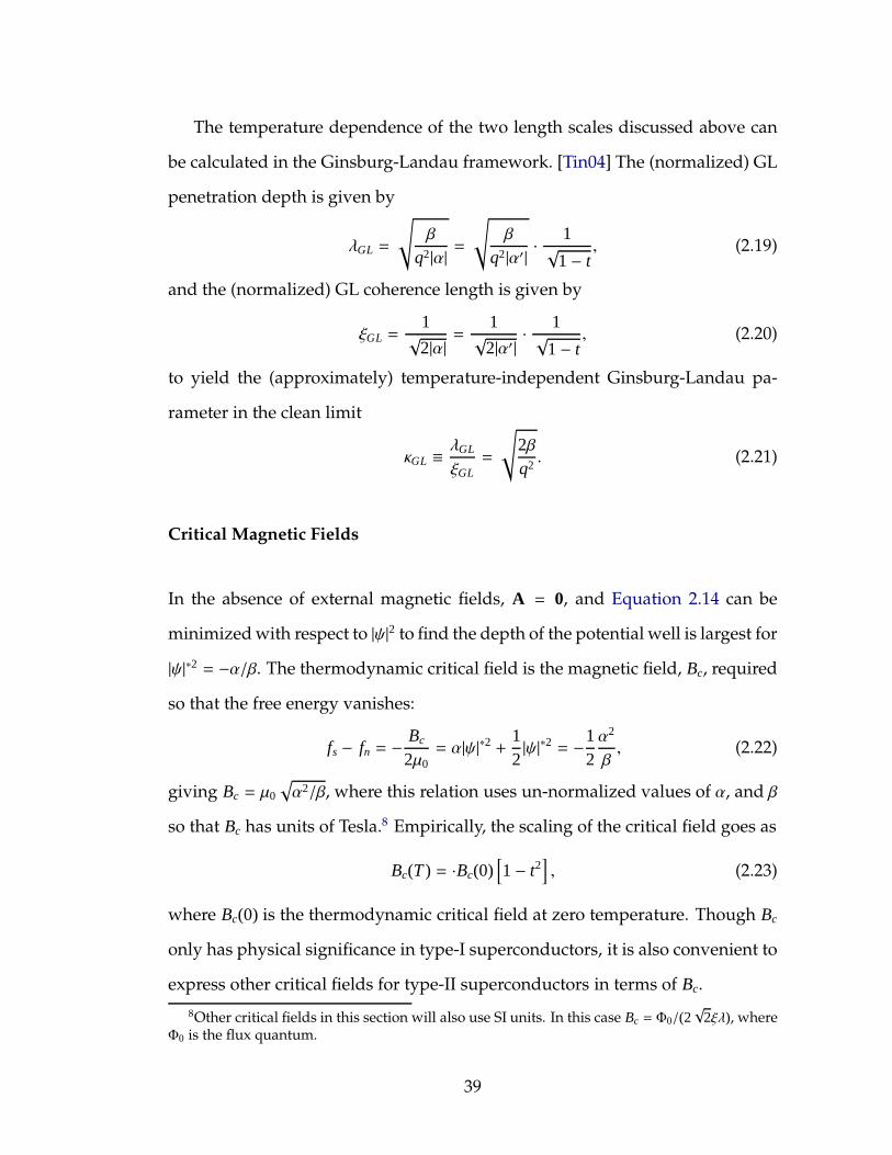
The temperature dependence of the two length scales discussed above can
be calculated in the Ginsburg-Landau framework. [Tin04] The (normalized) GL
penetration depth is given by
λGL =
√
β
q2|α| =√
β
q2|α′| ·1√1− t
, (2.19)
and the (normalized) GL coherence length is given by
ξGL =1√2|α|=
1√2|α′|
· 1√1− t
, (2.20)
to yield the (approximately) temperature-independent Ginsburg-Landau pa-
rameter in the clean limit
κGL ≡λGL
ξGL=
√
2βq2. (2.21)
Critical Magnetic Fields
In the absence of external magnetic fields, A = 0, and Equation 2.14 can be
minimized with respect to |ψ|2 to find the depth of the potential well is largest for
|ψ|∗2 = −α/β. The thermodynamic critical field is the magnetic field, Bc, required
so that the free energy vanishes:
fs − fn = −Bc
2µ0= α|ψ|∗2 + 1
2|ψ|∗2 = −1
2α2
β, (2.22)
giving Bc = µ0
√
α2/β, where this relation uses un-normalized values of α, and β
so that Bc has units of Tesla.8 Empirically, the scaling of the critical field goes as
Bc(T ) = ·Bc(0)[
1− t2]
, (2.23)
where Bc(0) is the thermodynamic critical field at zero temperature. Though Bc
only has physical significance in type-I superconductors, it is also convenient to
express other critical fields for type-II superconductors in terms of Bc.
8Other critical fields in this section will also use SI units. In this case Bc = Φ0/(2√
2ξλ), whereΦ0 is the flux quantum.
39
Figure 2.1: Flux line decoration of a high-purity Nb foil 0.16 mm thick at 1.2 K,with an applied field of 17.3 mT which is above Bc1 for the foil. Darkislands are vortex lines embedded in a Meissner phase. [Bra95]
For type-II materials, the lower critical field, Bc1, is the field at which the
Gibbs energy of the system is equivalent whether a magnetic flux line (vortex)
is inside or outside the superconductor. As such, this is the lowest field at which
a superconductor can enter a mixed state, illustrated in Figure 2.1. There is not
an exact closed form solution of Bc1 in terms of κGL, but for κ ≫ 1, it can be
approximately given by
Bc1 =Φ0
4πµ0λ2GL
log(κGL), (2.24)
where Φ0 = h/(2e) ≈ 2.07× 10⁻¹⁵ T·m is the flux quantum. [Tin04]
The dependence of Bc1 on κGL can be computed numerically from the
Ginsburg-Landau equations. [HA63]9 An approximate expression relating Bc1
and Bc,10 through the dependence on the Ginsburg-Landau parameter κGL was
9The reader is cautioned that the author of this paper interchanges the usual definition ofBc1, the lower critical field, and Bc2, the upper critical field, in his derivation.
10As mentioned, while Bc does not have physical significance for type-II superconductors,however Bc is approximately the geometric mean between Bc1 and Bc2. [Tin04]
40
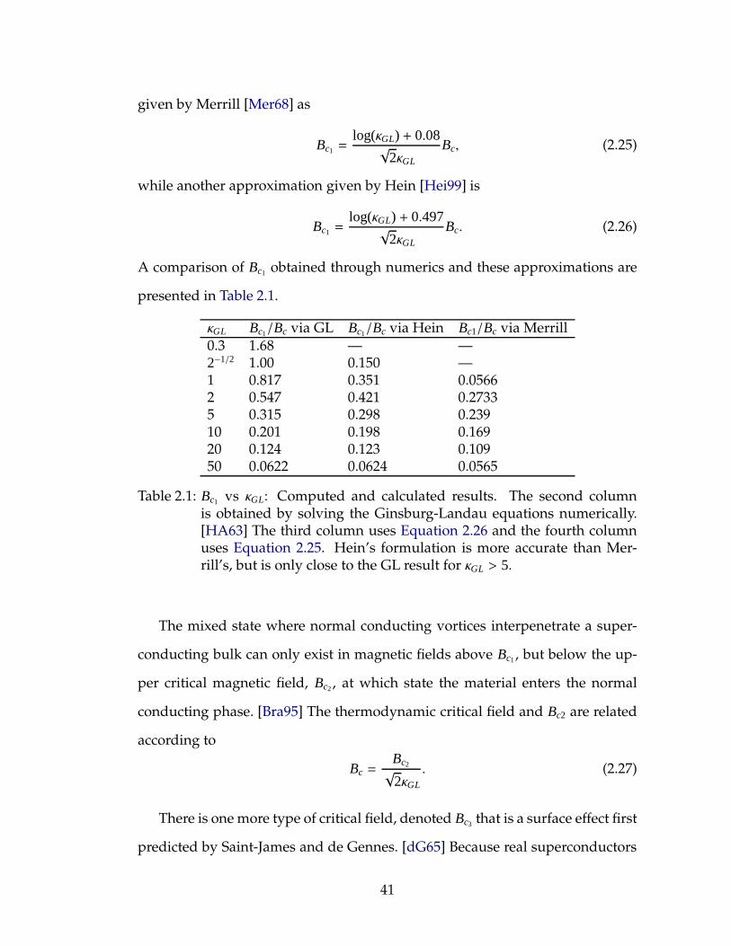
given by Merrill [Mer68] as
Bc1 =log(κGL) + 0.08√
2κGL
Bc, (2.25)
while another approximation given by Hein [Hei99] is
Bc1 =log(κGL) + 0.497√
2κGL
Bc. (2.26)
A comparison of Bc1 obtained through numerics and these approximations are
presented in Table 2.1.
κGL Bc1/Bc via GL Bc1/Bc via Hein Bc1/Bc via Merrill0.3 1.68 — —2−1/2 1.00 0.150 —1 0.817 0.351 0.05662 0.547 0.421 0.27335 0.315 0.298 0.23910 0.201 0.198 0.16920 0.124 0.123 0.10950 0.0622 0.0624 0.0565
Table 2.1: Bc1 vs κGL: Computed and calculated results. The second columnis obtained by solving the Ginsburg-Landau equations numerically.[HA63] The third column uses Equation 2.26 and the fourth columnuses Equation 2.25. Hein’s formulation is more accurate than Mer-rill’s, but is only close to the GL result for κGL > 5.
The mixed state where normal conducting vortices interpenetrate a super-
conducting bulk can only exist in magnetic fields above Bc1, but below the up-
per critical magnetic field, Bc2, at which state the material enters the normal
conducting phase. [Bra95] The thermodynamic critical field and Bc2 are related
according to
Bc =Bc2√2κGL
. (2.27)
There is one more type of critical field, denoted Bc3 that is a surface effect first
predicted by Saint-James and de Gennes. [dG65] Because real superconductors
41

are finite in size, the behaviour near the surfaces must be taken into account.
For fields parallel to a superconducting surface, above Bc2 superconductivity
can nucleate at a metal-insulator interfaces, though the bulk remains normal
conducting.
Both theory and experiment have shown that for fields parallel to the surface
of the bulk material of magnitude
Bc3 = 1.695Bc2, (2.28)
a superconducting surface sheath of thickness ξGL persists, while the bulk is
normal conducting. [FSS66] This field dominates a different type of phenomena
compared with the other critical fields, because of the depth dependence of the
state. For other critical fields, the superconductors have constant depth profiles,
either being in the Meissner state or normal conducting state, where as between
Bc2 and Bc3, there is a transition from the superconducting to normal conducting
state as depth increases.
For reference, Table 2.2 presents several values of critical fields for niobium
found in the literature.
2.2 The Superheating Field
Critical fields mentioned thus far are in equilibrium conditions. Before a transi-
tion takes place, there is an energy cost to nucleate a fluxoid, which leaves open
the possibility of a metastable state in which the energetically favorable transi-
tion has not occurred due to the activation energy barrier. This barrier vanishes
at the superheating field, Bsh.
42
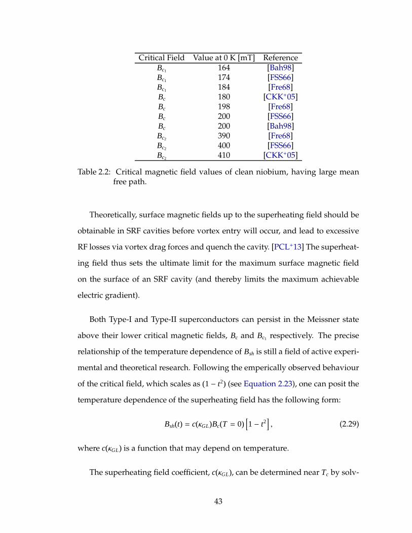
Critical Field Value at 0 K [mT] ReferenceBc1 164 [Bah98]Bc1 174 [FSS66]Bc1 184 [Fre68]Bc 180 [CKK+05]Bc 198 [Fre68]Bc 200 [FSS66]Bc 200 [Bah98]Bc2 390 [Fre68]Bc2 400 [FSS66]Bc2 410 [CKK+05]
Table 2.2: Critical magnetic field values of clean niobium, having large meanfree path.
Theoretically, surface magnetic fields up to the superheating field should be
obtainable in SRF cavities before vortex entry will occur, and lead to excessive
RF losses via vortex drag forces and quench the cavity. [PCL+13] The superheat-
ing field thus sets the ultimate limit for the maximum surface magnetic field
on the surface of an SRF cavity (and thereby limits the maximum achievable
electric gradient).
Both Type-I and Type-II superconductors can persist in the Meissner state
above their lower critical magnetic fields, Bc and Bc1 respectively. The precise
relationship of the temperature dependence of Bsh is still a field of active experi-
mental and theoretical research. Following the emperically observed behaviour
of the critical field, which scales as (1− t2) (see Equation 2.23), one can posit the
temperature dependence of the superheating field has the following form:
Bsh(t) = c(κGL)Bc(T = 0)[
1− t2]
, (2.29)
where c(κGL) is a function that may depend on temperature.
The superheating field coefficient, c(κGL), can be determined near Tc by solv-
43
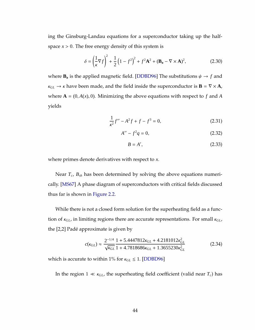
ing the Ginsburg-Landau equations for a superconductor taking up the half-
space x > 0. The free energy density of this system is
δ =
(
1κ∇ f
)2
+12
(
1− f 2)2+ f 2A2
+ (Ba − ∇ × A)2, (2.30)
where Ba is the applied magnetic field. [DDBD96] The substitutions ψ → f and
κGL → κ have been made, and the field inside the superconductor is B = ∇ × A,
where A = (0, A(x), 0). Minimizing the above equations with respect to f and A
yields
1κ2
f ′′ − A2 f + f − f 3= 0, (2.31)
A′′ − f 2q = 0, (2.32)
B = A′, (2.33)
where primes denote derivatives with respect to x.
Near Tc, Bsh has been determined by solving the above equations numeri-
cally. [MS67] A phase diagram of superconductors with critical fields discussed
thus far is shown in Figure 2.2.
While there is not a closed form solution for the superheating field as a func-
tion of κGL, in limiting regions there are accurate representations. For small κGL,
the [2,2] Pade approximate is given by
c(κGL) ≈ 2−1/4
√κGL
1+ 5.4447812κGL + 4.2181012κ2GL
1+ 4.7818686κGL + 1.3655230κ2GL
(2.34)
which is accurate to within 1% for κGL ≤ 1. [DDBD96]
In the region 1 ≪ κGL, the superheating field coefficient (valid near Tc) has
44

0 0.5 1 1.5 20
0.5
1
1.5
2
2.5
3
κGL
B/B
c
Bc2/Bc
Bc1/Bc
Bsh/Bc
Meissner State
Superheated State
Mixed StateNormal State
Nio
biu
m
Lea
d
Figure 2.2: Phase diagram of normalized magnetic field vs κGL for supercon-ductors in the intermediate κGL range at T = Tc. Note that abovethe Meissner state for both Type-I and Type-II superconductors, ametastable superheating state exists up to the superheating fieldthat, in the equilibrium state, would be either a normal conductingor mixed state. The line showing the superheating field was solvednumerically by Matricon and Saint-James. [MS67] Dashed lines marktypical values of κGL for clean Pb and Nb.
the form
c(κGL) ≈√
53+
89
(
215
)1/4 z3/40√κGL
(2.35)
≈√
53+
0.544755√κGL
(2.36)
where z0 ≈ 1.018793is the smallest number satisfying Ai’(−z0) = 0; [TCS11] Ai(x)
is the Airy function satisfying the differential equation y′′ − xy = 0. [Abr70, p.
446]
The most recent and thorough treatment of Ginsburg-Landau equations
solved them over a large range of κ to yield the superheating field, Bsh, taking
45
into account one- and two-dimensional perturbations causing the instability of
the Meissner phase. [TCS11] This solution yields the correct values of the su-
perheating field, which Equation 2.34 and Equation 2.35 approximate, in their
realms of validity, to within a few percent.
The phenomenological approach gives insight into Bsh near Tc but to inves-
tigate its behaviour over a range of temperatures, a more physically complete
theory is required. In general one expects the behavior of the critical fields as a
function of temperature to behave qualitatively as illustrated in Figure 2.3. The
essential feature of the figure is the demonstration that the typical SRF accelera-
tor operating region is far from the region where GL theory is applicable, calling
for a thorough theoretical and experimental treatment of the superheating field
and its full temperature dependence.
In principle BCS theory allows a complete understanding of the temperature
dependence of the superheating field. In practice, however, currently it is not
known how to compute the superheating field within this context, nor even how
to correctly formulate the problem. Thus, another simpler theory is necessary
to make progress on this front.
To this end, two methods, the Eilenberger equations and Eliashberg the-
ory, allow determination of the superheating field as a function of tempera-
ture. Eliashberg theory [GE68] requires the full information about the electronic
structure of the superconductor and is very difficult to solve. The Eilenberger
equations, [Eil68] while also very challenging to solve, have been the subject
of significant recent theoretical progress, and thus provide the best theoretical
understanding to date. The temperature dependence of the superheating field
prefactor, c(κGL, T ), was solved in the high-κ limit for strongly type-II supercon-
46
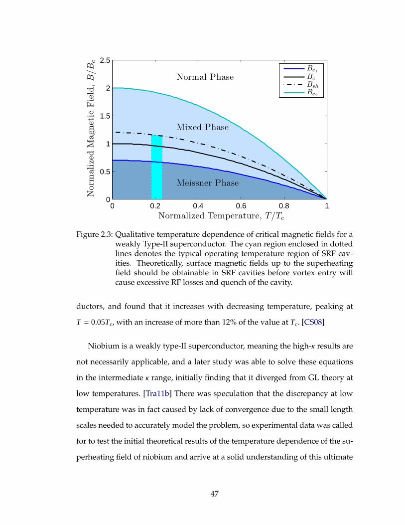
Normalized Temperature, T/Tc
Norm
alize
dM
agnet
icF
ield
,B
/B
c
Meissner Phase
Mixed Phase
Normal Phase
0 0.2 0.4 0.6 0.8 10
0.5
1
1.5
2
2.5Bc1
Bc
Bsh
Bc2
Figure 2.3: Qualitative temperature dependence of critical magnetic fields for aweakly Type-II superconductor. The cyan region enclosed in dottedlines denotes the typical operating temperature region of SRF cav-ities. Theoretically, surface magnetic fields up to the superheatingfield should be obtainable in SRF cavities before vortex entry willcause excessive RF losses and quench of the cavity.
ductors, and found that it increases with decreasing temperature, peaking at
T = 0.05Tc, with an increase of more than 12% of the value at Tc. [CS08]
Niobium is a weakly type-II superconductor, meaning the high-κ results are
not necessarily applicable, and a later study was able to solve these equations
in the intermediate κ range, initially finding that it diverged from GL theory at
low temperatures. [Tra11b] There was speculation that the discrepancy at low
temperature was in fact caused by lack of convergence due to the small length
scales needed to accurately model the problem, so experimental data was called
for to test the initial theoretical results of the temperature dependence of the su-
perheating field of niobium and arrive at a solid understanding of this ultimate
47

limit for SRF cavities at low temperatures.
2.3 Review of Superheating Field Experiments
Much of the experimental understanding of the superheating field has been
through using the RF critical field (BRFc ), or largest RF magnetic field that can
be applied to a sample while it remains superconducting, as a proxy for the su-
perheating field. The reason these fields may not be equivalent is that the critical
RF field can be limited by material defects, local roughness, surface contamina-
tion or pre-quench heating causing superconductivity to quench at prematurely
low fields. For a perfect sample, however, one would expect that the critical RF
field is limited only by Bsh since that is a fundamental property of the material.
Above this field, vortices enter the material, and large vortex drag in the RF field
will generate excessive heating and leading to quench and phase transition, so
fields above the superheating field with superconductor in a mixed state can not
be reaching in GHz RF field cavities.
Finnemore et al. measured Bc, Bc1 and Bc2 for high purity samples of nio-
bium using magnetization curves and noted that when measuring Bc1, “a final,
steady-state value of the magnetization is sometimes obtained only after 10 or
20 sample translations. It is as if vibration assists the flux movement into or out
of the sample.” [FSS66] Though they did not assert that the field values in the
Meissner state above the final measured Bc1 were evidence of superheating, it
seems likely. A similar set-up was used by Doll and Graf to measure the su-
perheating in Sn samples [DG67], though their measurements were only over a
small temperature range near Tc.
48
The first measurement confirming that the superheating field of niobium is
greater than the thermodynamic critical field, Bc was reported in 1967 by Renard
and Rocher [RR67]. They used magnetization curves of very pure Nb cylinders
at 4.2K to demonstrate this fact, and set the stage for subsequent measurements.
2.3.1 Superheating measured near Tc as a function of κ
The superheating field near the critical temperature, Tc, has been measured for
several Type-I materials, such as In, Sn, and Pb, as well as with a few alloys of
SnIn and InBi that are Type-II. [YDM77] For these measurements, a supercon-
ducting Nb resonator was used to generate large RF magnetic fields on samples,
defining BRFc as the field at which the resonator Q was degraded by dissipation
in the sample. [YDM77]
A plot of the phase diagram along with several measurements of critical RF
fields are presented in Figure 2.4.
Yogi did not study the temperature variation of the superheating field, and
was only done at temperatures just under Tc, at RF frequencies ranging between
90 and 300 MHz.
Yogi used measurements of several types of materials with κGL near to Tc
to try to determine the type of nucleation of normal conducting sites above
Bsh. [YDM77] He used his data to compare several models: A ”plane nucleation
model” into the spherical samples will cause Bsh to scale with (1−t)−1/12, [SBC70],
where as ”line nucleation model” would scale with (1− t)−1/6, and point nucle-
ation would scale with (1− t)−1/4. [YDM77]
49
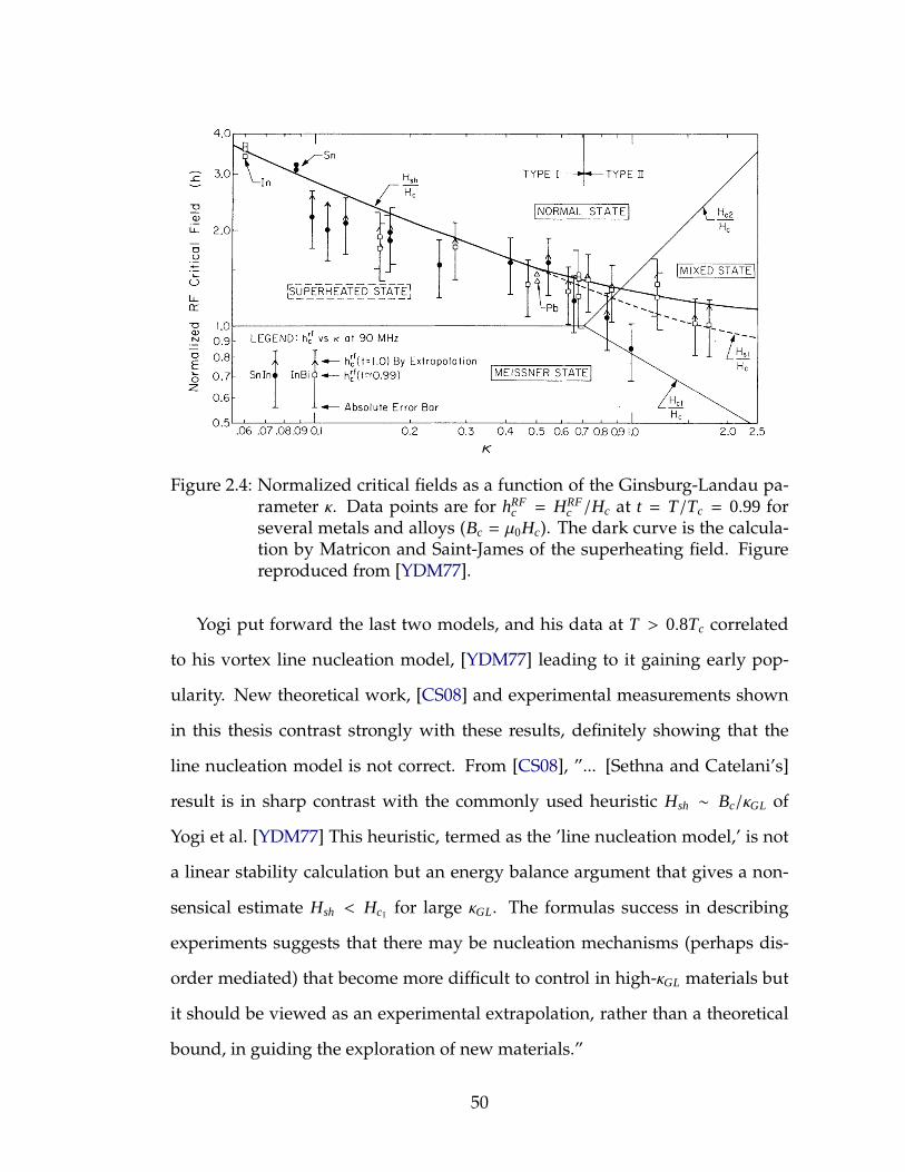
Figure 2.4: Normalized critical fields as a function of the Ginsburg-Landau pa-rameter κ. Data points are for hRF
c = HRFc /Hc at t = T/Tc = 0.99 for
several metals and alloys (Bc = µ0Hc). The dark curve is the calcula-tion by Matricon and Saint-James of the superheating field. Figurereproduced from [YDM77].
Yogi put forward the last two models, and his data at T > 0.8Tc correlated
to his vortex line nucleation model, [YDM77] leading to it gaining early pop-
ularity. New theoretical work, [CS08] and experimental measurements shown
in this thesis contrast strongly with these results, definitely showing that the
line nucleation model is not correct. From [CS08], ”... [Sethna and Catelani’s]
result is in sharp contrast with the commonly used heuristic Hsh ∼ Bc/κGL of
Yogi et al. [YDM77] This heuristic, termed as the ’line nucleation model,’ is not
a linear stability calculation but an energy balance argument that gives a non-
sensical estimate Hsh < Hc1 for large κGL. The formulas success in describing
experiments suggests that there may be nucleation mechanisms (perhaps dis-
order mediated) that become more difficult to control in high-κGL materials but
it should be viewed as an experimental extrapolation, rather than a theoretical
bound, in guiding the exploration of new materials.”
50
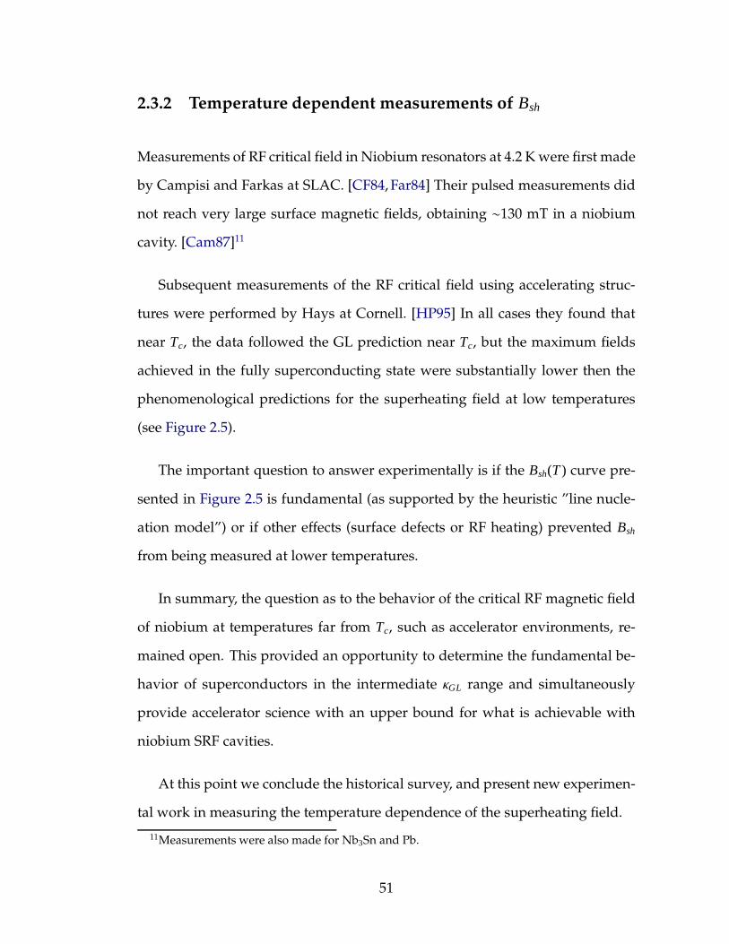
2.3.2 Temperature dependent measurements of Bsh
Measurements of RF critical field in Niobium resonators at 4.2 K were first made
by Campisi and Farkas at SLAC. [CF84, Far84] Their pulsed measurements did
not reach very large surface magnetic fields, obtaining ∼130 mT in a niobium
cavity. [Cam87]11
Subsequent measurements of the RF critical field using accelerating struc-
tures were performed by Hays at Cornell. [HP95] In all cases they found that
near Tc, the data followed the GL prediction near Tc, but the maximum fields
achieved in the fully superconducting state were substantially lower then the
phenomenological predictions for the superheating field at low temperatures
(see Figure 2.5).
The important question to answer experimentally is if the Bsh(T ) curve pre-
sented in Figure 2.5 is fundamental (as supported by the heuristic ”line nucle-
ation model”) or if other effects (surface defects or RF heating) prevented Bsh
from being measured at lower temperatures.
In summary, the question as to the behavior of the critical RF magnetic field
of niobium at temperatures far from Tc, such as accelerator environments, re-
mained open. This provided an opportunity to determine the fundamental be-
havior of superconductors in the intermediate κGL range and simultaneously
provide accelerator science with an upper bound for what is achievable with
niobium SRF cavities.
At this point we conclude the historical survey, and present new experimen-
tal work in measuring the temperature dependence of the superheating field.
11Measurements were also made for Nb3Sn and Pb.
51
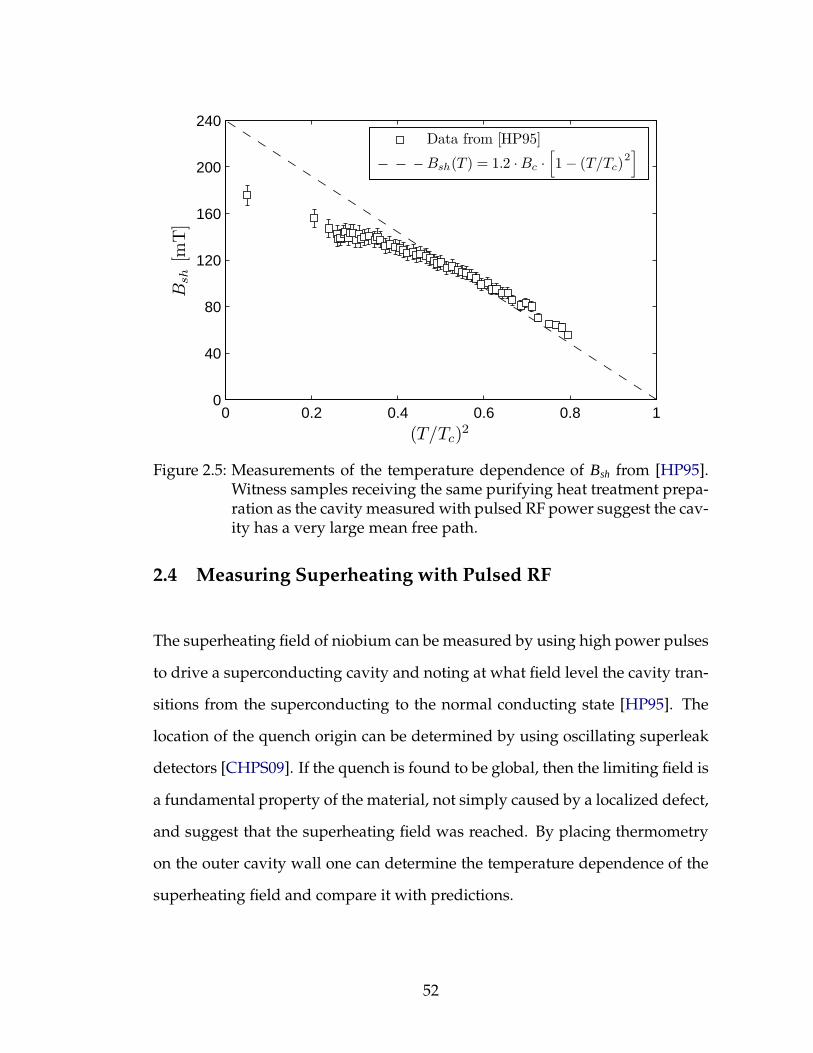
0 0.2 0.4 0.6 0.8 10
40
80
120
160
200
240
(T/Tc)2
Bsh
[mT
]
Data from [HP95]
Bsh(T) = 1.2 ·Bc ·[
1− (T/Tc)2]
Figure 2.5: Measurements of the temperature dependence of Bsh from [HP95].Witness samples receiving the same purifying heat treatment prepa-ration as the cavity measured with pulsed RF power suggest the cav-ity has a very large mean free path.
2.4 Measuring Superheating with Pulsed RF
The superheating field of niobium can be measured by using high power pulses
to drive a superconducting cavity and noting at what field level the cavity tran-
sitions from the superconducting to the normal conducting state [HP95]. The
location of the quench origin can be determined by using oscillating superleak
detectors [CHPS09]. If the quench is found to be global, then the limiting field is
a fundamental property of the material, not simply caused by a localized defect,
and suggest that the superheating field was reached. By placing thermometry
on the outer cavity wall one can determine the temperature dependence of the
superheating field and compare it with predictions.
52
By calculating the quality factor–a number proportional to how many RF
cycles it takes to dissipate the energy stored in a system–during the pulse, one
can pinpoint the time the cavity transitioned into the normal conducting state.
The surface magnetic fields at the transition time yield the superheating field.
To accurately measure the superheating field, it is essential to determine pre-
cisely when the cavity transitions to the normal conducting state. Previous work
has shown that a niobium cavity remains at least 90% superconducting as long
as the intrinsic quality factor is greater than 2× 10⁶. [HPR95,HP95]12 It has been
shown how to determine the quality factor as a function of time in several pub-
lications, [Far84, CF84, HPR95, HP95] but the argument is reproduced here for
completeness.
A cavity with a resonant frequency, ω, driven on resonance by a single input
coupler at power, P f , reflects some power, Pr, and has some power coupled
into the cavity, Pin. Part of the incident power wave increases the field in the
cavity, U, and part of the power is dissipated in the cavity walls, ωU/Q0, (see
Equation 1.9) where Q0 is the intrinsic quality factor of the cavity. Conservation
of energy gives:
P f = Pr + Pin, (2.37)
Pin =ωUQ0+
dUdt, (2.38)
where t is the time variable.
The reflected power is not a measured quantity in our experiment, so an-
12For high RRR material (RRR∼300), normal conducting Q0 at cryogenic temperatures areapproximately 2×10⁵. Assuming 20% of the material is normal conducting (90% has Q0 ≫ 108),the overall Q0 will be 2× 10⁶. The quality factor drops very quickly once the material begins tobecome normal conducting (see Figure 2.6), so the exact value used here for Q0 to determine theloss of superconductivity is not important, which is to say an essentially equivalent critical fieldwould be measured with a different Q0 threshold criteria such as 107 or 106. Thus the exact Qvalue used for the superconducting/normal conducting transition does not effect the results.
53
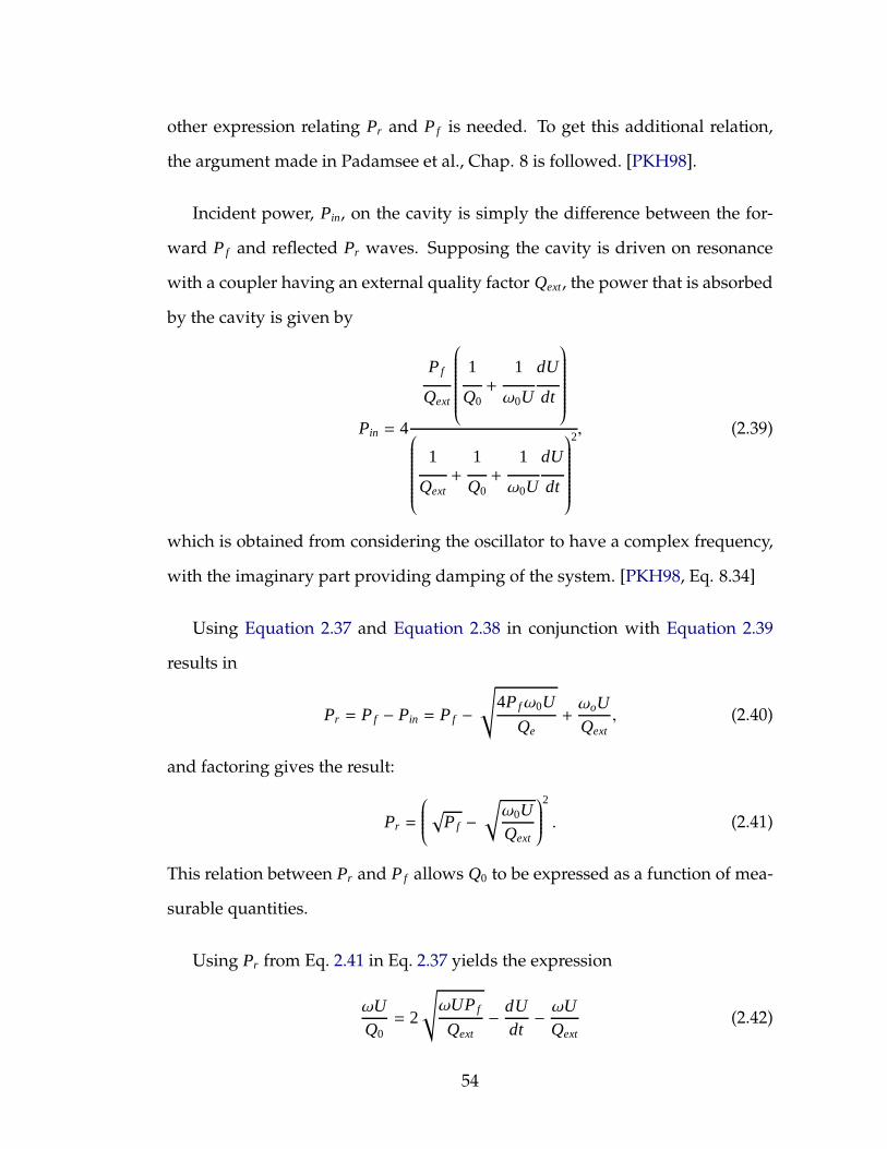
other expression relating Pr and P f is needed. To get this additional relation,
the argument made in Padamsee et al., Chap. 8 is followed. [PKH98].
Incident power, Pin, on the cavity is simply the difference between the for-
ward P f and reflected Pr waves. Supposing the cavity is driven on resonance
with a coupler having an external quality factor Qext , the power that is absorbed
by the cavity is given by
Pin = 4
P f
Qext
1
Q0+
1
ω0U
dU
dt
1
Qext+
1
Q0+
1
ω0U
dU
dt
2, (2.39)
which is obtained from considering the oscillator to have a complex frequency,
with the imaginary part providing damping of the system. [PKH98, Eq. 8.34]
Using Equation 2.37 and Equation 2.38 in conjunction with Equation 2.39
results in
Pr = P f − Pin = P f −√
4P fω0U
Qe+ωoUQext
, (2.40)
and factoring gives the result:
Pr =
√
P f −√
ω0UQext
2
. (2.41)
This relation between Pr and P f allows Q0 to be expressed as a function of mea-
surable quantities.
Using Pr from Eq. 2.41 in Eq. 2.37 yields the expression
ωUQ0= 2
√
ωUP f
Qext− dU
dt− ωU
Qext(2.42)
54

The final expression relating Q0 and time can be obtained by using the identity
d√
Udt=
1
2√
U
dUdt, (2.43)
to yield
1Q0=
2
ω√
U
√
ωP f
Qext− d√
Udt
− 1
Qext(2.44)
Equation 2.44 allows one to calculate Q0 as a function of time from measure-
ments of P f and U. Finding the time when the quality factor of the cavity falls
bellow 2×10⁶ pinpoints when the cavity transitions into the normal conducting
state. [HPR95]
Two examples of the application of these equations to pulsed RF measure-
ments are presented in Figure 2.6 and Figure 2.7.
As a comparison between the two RF measurements shows, the supercon-
ducting to normal conducting transition field is not necessarily the maximum
surface field measured. This is because under certain conditions it is still pos-
sible to load the resonator with more power than it dissipates, while it is in the
normal conducting state. Therefore, Equation 2.44 is necessary to determine the
precise transition time.
2.4.1 Experimental Methods to Distinguish Bsh from BRFmax,sc
The superheating magnetic field is measured with a niobium resonator driven
by a klystron capable of supplying 1.5 MW pulses with durations between 50-
500 µs. These short, high power pulses are intended to minimize cavity heating
as the electro-magnetic fields increase, so the temperature across the cavity wall
is small.
55

0 50 100 150 2000
50
100
150
200
250
T = 2.96 K
Time [µs]
Surf
ace
magnet
icfiel
d[m
T]
103
104
105
106
107
108
Cav
ity
Q0
Pf
Bsurf
Q0
Figure 2.6: Superconducting to normal conducting transition field measure-ment at 2.96 K. The cavity’s Q0 shows the cavity enters the normalconducting state near the maximal measured surface field. Powersupplied to the cavity by the klystron, P f , is plotted in arbitraryunits, but has peak magnitude of ∼1 MW.
When the magnetic field on the cavity surface reaches the so-called quench
field, BRFmax,sc, the superconductor undergoes a phase transition into the normal
conducting state.13 There is no guarantee that this transition is initiated by ex-
ceeding the fundamental limitation of the superconductor, as many phenomena
can reduce the peak performance of superconducting material. One hint as to
the nature of the break down of superconductivity is the quench location.
If the break down down of superconductivity occurs in a localized region,
it is most likely due to contamination on the surface or a material defect. If the
quench occurs over a large region, it is likely that a fundamental limitation of
the superconductor has been reached, so that BRFmax,sc = Bsh.
13This transition dissipates a great deal of energy, and is often referred to as a quench.
56
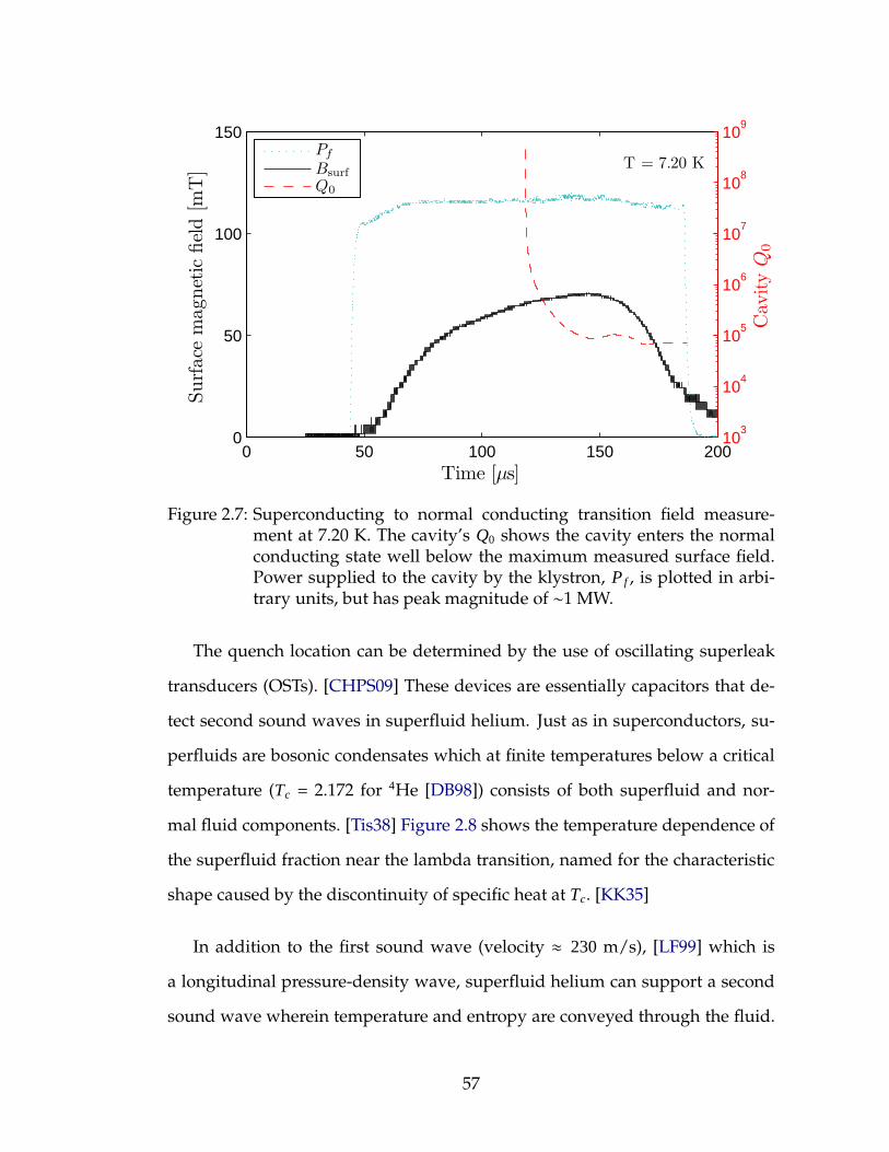
0 50 100 150 2000
50
100
150
T = 7.20 K
Time [µs]
Surf
ace
magnet
icfiel
d[m
T]
103
104
105
106
107
108
109
Cav
ity
Q0
Pf
Bsurf
Q0
Figure 2.7: Superconducting to normal conducting transition field measure-ment at 7.20 K. The cavity’s Q0 shows the cavity enters the normalconducting state well below the maximum measured surface field.Power supplied to the cavity by the klystron, P f , is plotted in arbi-trary units, but has peak magnitude of ∼1 MW.
The quench location can be determined by the use of oscillating superleak
transducers (OSTs). [CHPS09] These devices are essentially capacitors that de-
tect second sound waves in superfluid helium. Just as in superconductors, su-
perfluids are bosonic condensates which at finite temperatures below a critical
temperature (Tc = 2.172 for 4He [DB98]) consists of both superfluid and nor-
mal fluid components. [Tis38] Figure 2.8 shows the temperature dependence of
the superfluid fraction near the lambda transition, named for the characteristic
shape caused by the discontinuity of specific heat at Tc. [KK35]
In addition to the first sound wave (velocity ≈ 230 m/s), [LF99] which is
a longitudinal pressure-density wave, superfluid helium can support a second
sound wave wherein temperature and entropy are conveyed through the fluid.
57

2.16 2.164 2.168 2.172 2.1760
0.02
0.04
0.06
0.08
Temperature [K]
ρs/ρ
2.16 2.164 2.168 2.172 2.17620
35
50
65
80
Spec
ific
Hea
t[J
/K·m
ol]
Figure 2.8: Superfluid fraction () and specific heat () of 4He vs temperature.
[LFF47] The velocity of the second sound wave is temperature dependent (see
Figure 2.9), but does not vary much in the region used for SRF research.
An OST is essentially a capacitor with a semipermeable membrane on one
side that allows the superfluid component of helium to pass into the capacitor
while screening out the normal fluid component. The change in capacitance
when the 2nd sound wave arrives at the OST membrane can be measured on
an oscilloscope. By measuring the time delay between the dissipation of cavity
stored energy (quench) and the ringing of OSTs, trilateration can be performed
to determine the original quench location at a certain region on the cavity wall.
58
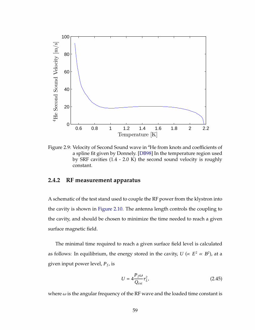
0.6 0.8 1 1.2 1.4 1.6 1.8 2 2.20
20
40
60
80
100
4H
eSec
ond
Sound
Vel
oci
ty[m
/s]
Temperature [K]
Figure 2.9: Velocity of Second Sound wave in 4He from knots and coefficients ofa spline fit given by Donnely. [DB98] In the temperature region usedby SRF cavities (1.4 - 2.0 K) the second sound velocity is roughlyconstant.
2.4.2 RF measurement apparatus
A schematic of the test stand used to couple the RF power from the klystron into
the cavity is shown in Figure 2.10. The antenna length controls the coupling to
the cavity, and should be chosen to minimize the time needed to reach a given
surface magnetic field.
The minimal time required to reach a given surface field level is calculated
as follows: In equilibrium, the energy stored in the cavity, U (∝ E2 ∝ B2), at a
given input power level, P f , is
U = 4P fω
Qextτ2
L, (2.45)
where ω is the angular frequency of the RF wave and the loaded time constant is
59
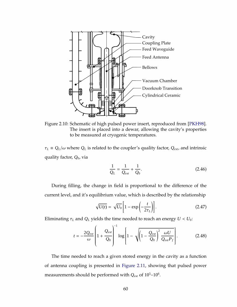
Figure 2.10: Schematic of high pulsed power insert, reproduced from [PKH98].The insert is placed into a dewar, allowing the cavity’s propertiesto be measured at cryogenic temperatures.
τL ≡ QL/ω where QL is related to the coupler’s quality factor, Qext , and intrinsic
quality factor, Q0, via
1QL=
1Qext+
1Q0. (2.46)
During filling, the change in field is proportional to the difference of the
current level, and it’s equilibrium value, which is described by the relationship
√
U(t) =√
U0
1− exp
(
− t2τL
)
. (2.47)
Eliminating τL and QL yields the time needed to reach an energy U < U0:
t = −2Qext
ω
1+Qext
Q0
−1
log
1−
√(
1− Qext
Q0
)2ωU
QextP f
. (2.48)
The time needed to reach a given stored energy in the cavity as a function
of antenna coupling is presented in Figure 2.11, showing that pulsed power
measurements should be performed with Qext of 105–106.
60

104
105
106
107
0
100
200
300
400
500
Tim
e[µ
s]
Qext
U = 5 JU = 10 JU = 15 JU = 20 JU = 25 JU = 30 JU = 35 J
Figure 2.11: Time needed to store a given amount of energy in the cavity vsantenna coupling. Equation 2.48 was used with ω = 2π · 1.3 GHz,Q0 = 1010 and P f = 1 MW. For comparison, in the cavity tested,LR1-3, 5 J ≈ 100 mT and 35 J ≈ 200 mT surface field.
Temperature Measurement
Temperatures of the cavity’s RF surface is determined by Cernox thermometers
on the outside wall. For short RF pulses, and high enough Q0, the temperature
gradient across the wall is very small. In addition, cooling grooves were milled
on the outside of the cavity to reduce the wall thickness and increase the heat
transfer to the liquid helium bath. For Q0 ∼ 109, the temperature difference
between the inner and outer wall is ∼0.2 K. [VCL09] However, if Q0 drops to low
values, the thermal gradient across the wall can become significant, preventing
Bsh from being reached at the bath temperature since the inner wall is at a higher
temperature.
61

2.4.3 Material Characterization via Q0 vs Temperature
It is desirable to characterize the material properties of the Nb surface to enable
correlation to superheating field results. This can be carried out by measuring
the surface resistivity of the superconductor as a function of temperature.
Holding the accelerating gradient constant, by measuring the intrinsic qual-
ity factor, Q0, as a function of temperature, the surface resistivity, Rs can be found
by using the relationship in Equation 1.14, Rs = G/Q0, where G is the geometry
factor of the cavity. This method requires the accelerating gradient to be large
enough to be out of the low field Q-slope region but not so large that medium-
or high-field Q-slope artificially reduces the quality factor.
In general, the surface resistance is the sum of two contributions: the BCS
resistance, which is temperature and frequency dependent, and the residual re-
sistance, which is temperature independent. After obtaining the surface resis-
tance, the material properties can be found by using a program SRIMP [Hal70b]
which yields the AC surface resistivity of a superconductor from parameters
using BCS theory. Further information about extracting superconducting prop-
erties from Rs vs temperature data is presented in Appendix C.
2.5 New Measurements of Bsh
A photograph of the niobium cavity, LR1-3, used in superheating field measure-
ments is shown in Figure 2.12. The cavity was outfitted with 8 OSTs to act as
quench detection and three Cernox temperature sensors attached to the outside
surface of the cavity.
62
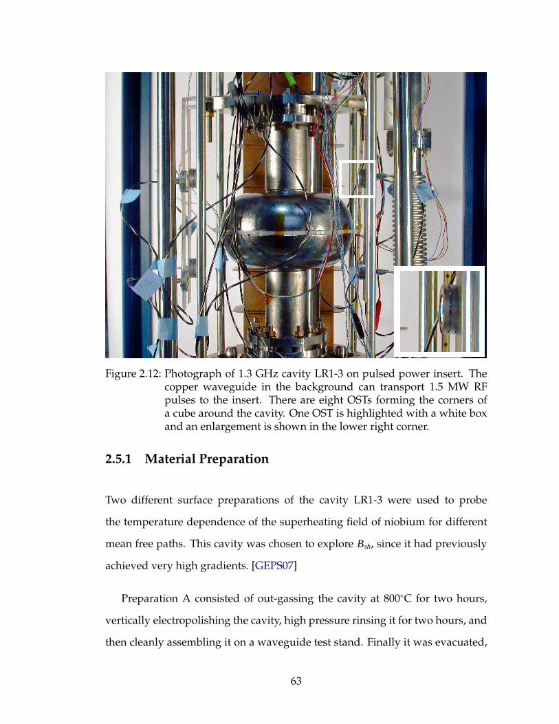
Figure 2.12: Photograph of 1.3 GHz cavity LR1-3 on pulsed power insert. Thecopper waveguide in the background can transport 1.5 MW RFpulses to the insert. There are eight OSTs forming the corners ofa cube around the cavity. One OST is highlighted with a white boxand an enlargement is shown in the lower right corner.
2.5.1 Material Preparation
Two different surface preparations of the cavity LR1-3 were used to probe
the temperature dependence of the superheating field of niobium for different
mean free paths. This cavity was chosen to explore Bsh, since it had previously
achieved very high gradients. [GEPS07]
Preparation A consisted of out-gassing the cavity at 800C for two hours,
vertically electropolishing the cavity, high pressure rinsing it for two hours, and
then cleanly assembling it on a waveguide test stand. Finally it was evacuated,
63
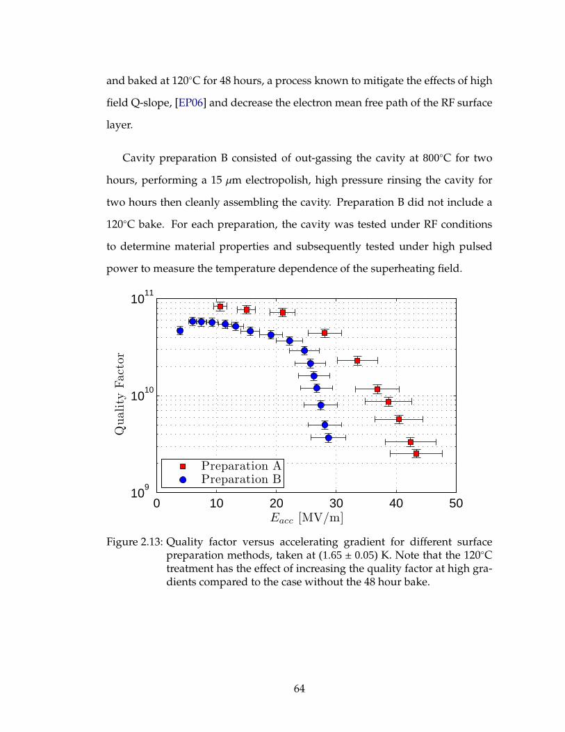
and baked at 120C for 48 hours, a process known to mitigate the effects of high
field Q-slope, [EP06] and decrease the electron mean free path of the RF surface
layer.
Cavity preparation B consisted of out-gassing the cavity at 800C for two
hours, performing a 15 µm electropolish, high pressure rinsing the cavity for
two hours then cleanly assembling the cavity. Preparation B did not include a
120C bake. For each preparation, the cavity was tested under RF conditions
to determine material properties and subsequently tested under high pulsed
power to measure the temperature dependence of the superheating field.
0 10 20 30 40 5010
9
1010
1011
Eacc [MV/m]
Quality
Fact
or
Preparation APreparation B
Figure 2.13: Quality factor versus accelerating gradient for different surfacepreparation methods, taken at (1.65± 0.05) K. Note that the 120Ctreatment has the effect of increasing the quality factor at high gra-dients compared to the case without the 48 hour bake.
64
2.5.2 Continuous Wave Measurements
The cavity’s properties were first tested in continuous wave (CW) mode. The
intrinsic quality factor, Q0, in both cases as a function of accelerating gradient is
shown in Figure 2.13. Both measurements demonstrate a strong decrease in Q0
(i.e. increase in surface resistivity) at high fields, though the cavity with Prepara-
tion A has a much higher quality factor above 30 MV/m. Neither measurement
was quench limited, but limited by the power available from the RF amplifier
driving the cavity.
The measurement of the quality factor vs temperature yielded the surface
resistance plots presented in Figure 2.14 via the use of Equation 1.14. For LR1-3,
G = 283.1Ω.
The Rs versus temperature data was used to extract material surface proper-
ties using SRIMP, as discussed in Appendix C. The critical temperature was de-
termined from pulsed superheating field measurements (presented in the next
section) to reduce the number of free parameters in the data fit. Material prop-
erties consistent with both measurements are presented in Table 2.3.
Using the material properties to estimate the GL parameter, κGL, for Prepa-
ration A, κGL = 3.52± 1.56, whereas for Preparation B, κGL = 1.25± 0.17. Solving
GL theory for the superheating field near Tc yields c(κGL) = 1.04±0.06 for Prepa-
ration A and c(κGL) = 1.22± 0.02 for Preparation B.14
The results are summarized in Table 2.3, demonstrating that the properties of
superconducting surface depends strongly on the material preparation. Prepa-
14The superheating field coefficient c(κGL) was calculated using interpolated values from 1Dand 2D stability analyses. [Tra11a]
65

1.4 2 2.6 3.2 3.8 4.410
−9
10−8
10−7
10−6
Temperature [K]
Surf
ace
Res
ista
nce
[Ω]
SRIMP PredictionPreparation APreparation B
Figure 2.14: Surface resistance versus temperature for the two different surfacepreparation methods. The black lines are the result of the BCS pre-diction generated by parameters presented in Table 2.3. The super-heating field coefficient was interpolated from 1D and 2D stabilityanalyses performed by M. Transtrum. [Tra11a]
ration A yielded a surface with larger κ, which is to say that it is more strongly
Type-II. Preparation B, however resulted in a surface with smaller κ, and the
Niobium is closer to Type-I in this case.
A few comments about the material properties obtained by these fits should
be mentioned: The energy gap, 2∆(0)/kB, of the niobium treated by Prepara-
tion A is larger than the reported value of 3.93 for pure niobium. [PKH98] The
surface preparation, especially the baking process, has been shown to effect the
energy gap, [Cio07] which could explain the difference in energy gap. The criti-
cal temperature of the sample significantly differs from the critical temperature
of pure niobium, 9.22 K, but is consistent with the diffusion of oxygen into the
superconductor, due to the low temperature bake. Assuming the degradation
66
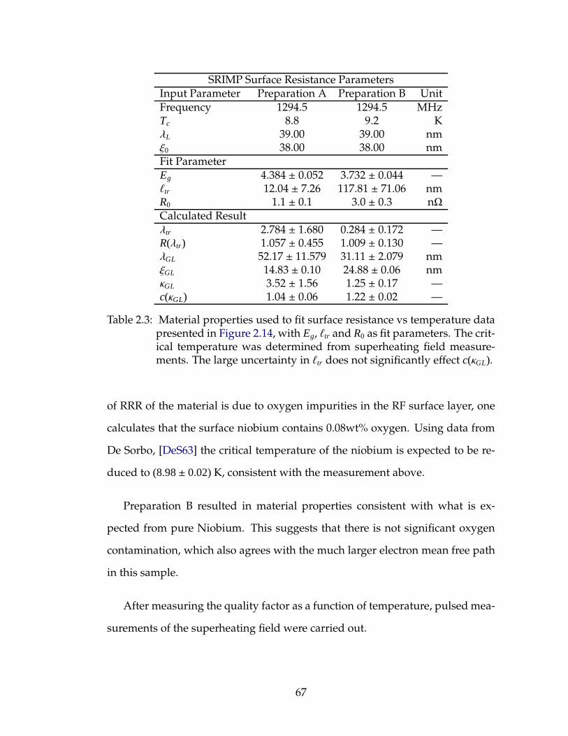
SRIMP Surface Resistance ParametersInput Parameter Preparation A Preparation B UnitFrequency 1294.5 1294.5 MHzTc 8.8 9.2 KλL 39.00 39.00 nmξ0 38.00 38.00 nmFit ParameterEg 4.384 ± 0.052 3.732 ± 0.044 —ℓtr 12.04 ± 7.26 117.81 ± 71.06 nmR0 1.1 ± 0.1 3.0 ± 0.3 nΩCalculated Resultλtr 2.784 ± 1.680 0.284 ± 0.172 —R(λtr) 1.057 ± 0.455 1.009 ± 0.130 —λGL 52.17 ± 11.579 31.11 ± 2.079 nmξGL 14.83 ± 0.10 24.88 ± 0.06 nmκGL 3.52 ± 1.56 1.25 ± 0.17 —c(κGL) 1.04 ± 0.06 1.22 ± 0.02 —
Table 2.3: Material properties used to fit surface resistance vs temperature datapresented in Figure 2.14, with Eg, ℓtr and R0 as fit parameters. The crit-ical temperature was determined from superheating field measure-ments. The large uncertainty in ℓtr does not significantly effect c(κGL).
of RRR of the material is due to oxygen impurities in the RF surface layer, one
calculates that the surface niobium contains 0.08wt% oxygen. Using data from
De Sorbo, [DeS63] the critical temperature of the niobium is expected to be re-
duced to (8.98± 0.02)K, consistent with the measurement above.
Preparation B resulted in material properties consistent with what is ex-
pected from pure Niobium. This suggests that there is not significant oxygen
contamination, which also agrees with the much larger electron mean free path
in this sample.
After measuring the quality factor as a function of temperature, pulsed mea-
surements of the superheating field were carried out.
67
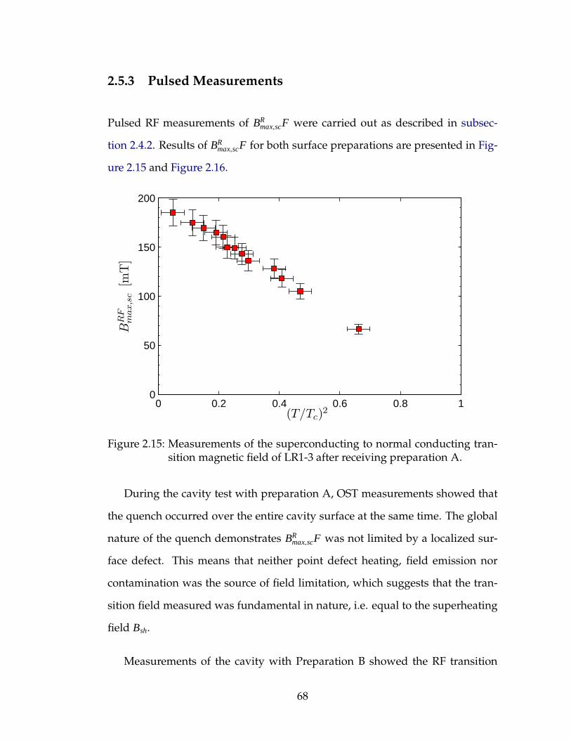
2.5.3 Pulsed Measurements
Pulsed RF measurements of BRmax,scF were carried out as described in subsec-
tion 2.4.2. Results of BRmax,scF for both surface preparations are presented in Fig-
ure 2.15 and Figure 2.16.
0 0.2 0.4 0.6 0.8 10
50
100
150
200
(T/Tc)2
BR
Fm
ax,s
c[m
T]
Figure 2.15: Measurements of the superconducting to normal conducting tran-sition magnetic field of LR1-3 after receiving preparation A.
During the cavity test with preparation A, OST measurements showed that
the quench occurred over the entire cavity surface at the same time. The global
nature of the quench demonstrates BRmax,scF was not limited by a localized sur-
face defect. This means that neither point defect heating, field emission nor
contamination was the source of field limitation, which suggests that the tran-
sition field measured was fundamental in nature, i.e. equal to the superheating
field Bsh.
Measurements of the cavity with Preparation B showed the RF transition
68
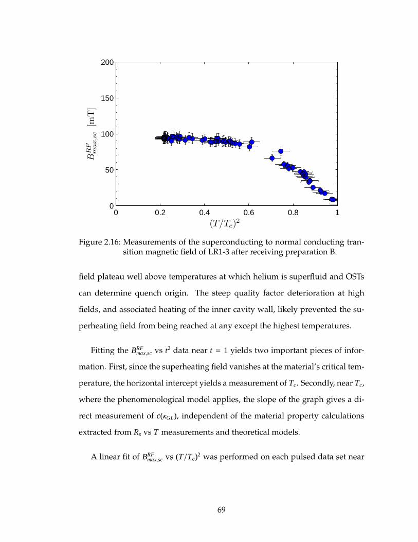
0 0.2 0.4 0.6 0.8 10
50
100
150
200
(T/Tc)2
BR
Fm
ax,s
c[m
T]
Figure 2.16: Measurements of the superconducting to normal conducting tran-sition magnetic field of LR1-3 after receiving preparation B.
field plateau well above temperatures at which helium is superfluid and OSTs
can determine quench origin. The steep quality factor deterioration at high
fields, and associated heating of the inner cavity wall, likely prevented the su-
perheating field from being reached at any except the highest temperatures.
Fitting the BRFmax,sc vs t2 data near t = 1 yields two important pieces of infor-
mation. First, since the superheating field vanishes at the material’s critical tem-
perature, the horizontal intercept yields a measurement of Tc. Secondly, near Tc,
where the phenomenological model applies, the slope of the graph gives a di-
rect measurement of c(κGL), independent of the material property calculations
extracted from Rs vs T measurements and theoretical models.
A linear fit of BRFmax,sc vs (T/Tc)2 was performed on each pulsed data set near
69
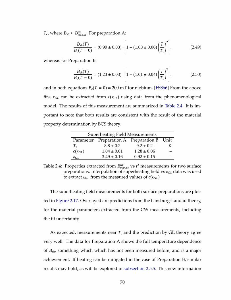
Tc, where Bsh ≈ BRFmax,sc. For preparation A:
Bsh(T )Bc(T = 0)
= (0.99± 0.03) ·
1− (1.08± 0.06)
(
TTc
)2
, (2.49)
whereas for Preparation B:
Bsh(T )Bc(T = 0)
= (1.23± 0.03) ·
1− (1.01± 0.04)
(
TTc
)2
, (2.50)
and in both equations Bc(T = 0) = 200 mT for niobium. [FSS66] From the above
fits, κGL can be extracted from c(κGL) using data from the phenomenological
model. The results of this measurement are summarized in Table 2.4. It is im-
portant to note that both results are consistent with the result of the material
property determination by BCS theory.
Superheating Field MeasurementsParameter Preparation A Preparation B UnitTc 8.8± 0.2 9.2± 0.2 Kc(κGL) 1.04± 0.01 1.28± 0.06 –κGL 3.49± 0.16 0.92± 0.15 –
Table 2.4: Properties extracted from BRFmax,sc vs t2 measurements for two surface
preparations. Interpolation of superheating field vs κGL data was usedto extract κGL from the measured values of c(κGL).
The superheating field measurements for both surface preparations are plot-
ted in Figure 2.17. Overlayed are predictions from the Ginsburg-Landau theory,
for the material parameters extracted from the CW measurements, including
the fit uncertainty.
As expected, measurements near Tc and the prediction by GL theory agree
very well. The data for Preparation A shows the full temperature dependence
of Bsh, something which which has not been measured before, and is a major
achievement. If heating can be mitigated in the case of Preparation B, similar
results may hold, as will be explored in subsection 2.5.5. This new information
70
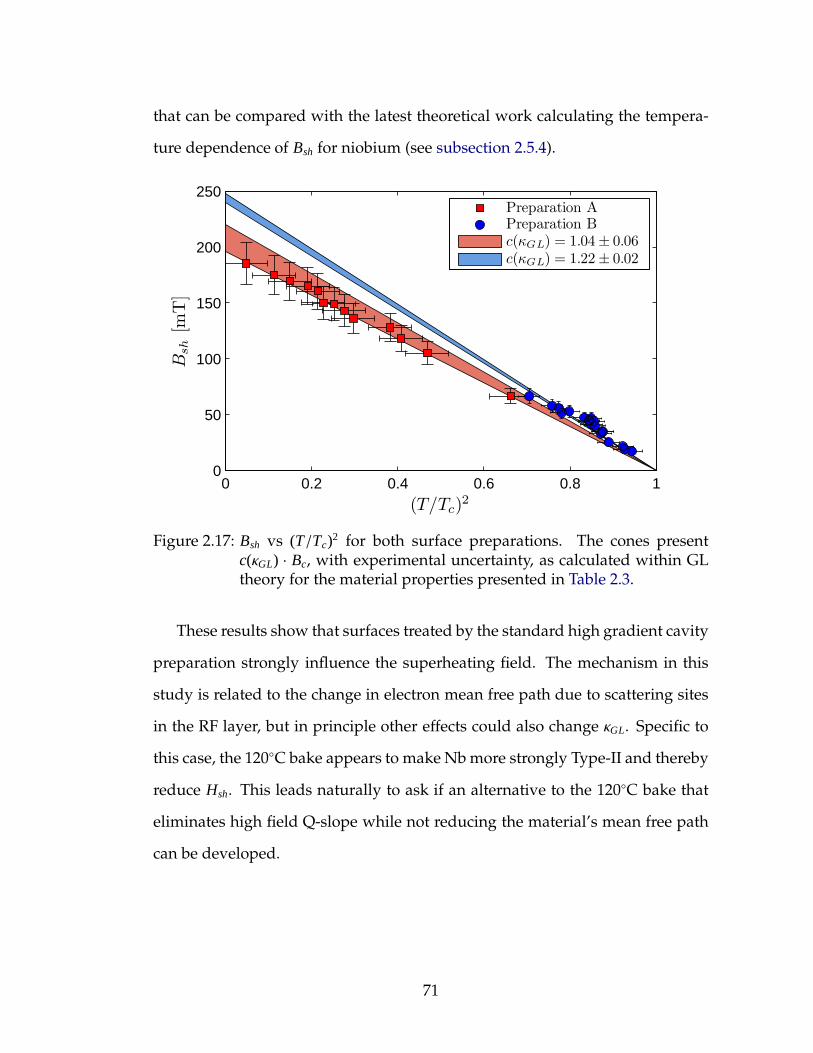
that can be compared with the latest theoretical work calculating the tempera-
ture dependence of Bsh for niobium (see subsection 2.5.4).
0 0.2 0.4 0.6 0.8 10
50
100
150
200
250
(T/Tc)2
Bsh
[mT
]
Preparation APreparation Bc(κGL) = 1.04± 0.06c(κGL) = 1.22± 0.02
Figure 2.17: Bsh vs (T/Tc)2 for both surface preparations. The cones presentc(κGL) · Bc, with experimental uncertainty, as calculated within GLtheory for the material properties presented in Table 2.3.
These results show that surfaces treated by the standard high gradient cavity
preparation strongly influence the superheating field. The mechanism in this
study is related to the change in electron mean free path due to scattering sites
in the RF layer, but in principle other effects could also change κGL. Specific to
this case, the 120C bake appears to make Nb more strongly Type-II and thereby
reduce Hsh. This leads naturally to ask if an alternative to the 120C bake that
eliminates high field Q-slope while not reducing the material’s mean free path
can be developed.
71
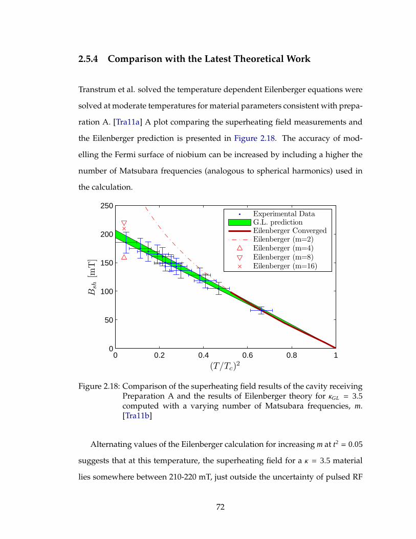
2.5.4 Comparison with the Latest Theoretical Work
Transtrum et al. solved the temperature dependent Eilenberger equations were
solved at moderate temperatures for material parameters consistent with prepa-
ration A. [Tra11a] A plot comparing the superheating field measurements and
the Eilenberger prediction is presented in Figure 2.18. The accuracy of mod-
elling the Fermi surface of niobium can be increased by including a higher the
number of Matsubara frequencies (analogous to spherical harmonics) used in
the calculation.
0 0.2 0.4 0.6 0.8 10
50
100
150
200
250
(T/Tc)2
Bsh
[mT
]
Experimental DataG.L. predictionEilenberger ConvergedEilenberger (m=2)Eilenberger (m=4)Eilenberger (m=8)Eilenberger (m=16)
Figure 2.18: Comparison of the superheating field results of the cavity receivingPreparation A and the results of Eilenberger theory for κGL = 3.5computed with a varying number of Matsubara frequencies, m.[Tra11b]
Alternating values of the Eilenberger calculation for increasing m at t2= 0.05
suggests that at this temperature, the superheating field for a κ = 3.5 material
lies somewhere between 210-220 mT, just outside the uncertainty of pulsed RF
72
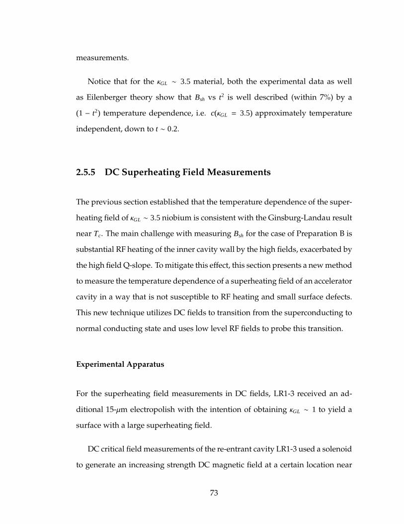
measurements.
Notice that for the κGL ∼ 3.5 material, both the experimental data as well
as Eilenberger theory show that Bsh vs t2 is well described (within 7%) by a
(1 − t2) temperature dependence, i.e. c(κGL = 3.5) approximately temperature
independent, down to t ∼ 0.2.
2.5.5 DC Superheating Field Measurements
The previous section established that the temperature dependence of the super-
heating field of κGL ∼ 3.5 niobium is consistent with the Ginsburg-Landau result
near Tc. The main challenge with measuring Bsh for the case of Preparation B is
substantial RF heating of the inner cavity wall by the high fields, exacerbated by
the high field Q-slope. To mitigate this effect, this section presents a new method
to measure the temperature dependence of a superheating field of an accelerator
cavity in a way that is not susceptible to RF heating and small surface defects.
This new technique utilizes DC fields to transition from the superconducting to
normal conducting state and uses low level RF fields to probe this transition.
Experimental Apparatus
For the superheating field measurements in DC fields, LR1-3 received an ad-
ditional 15-µm electropolish with the intention of obtaining κGL ∼ 1 to yield a
surface with a large superheating field.
DC critical field measurements of the re-entrant cavity LR1-3 used a solenoid
to generate an increasing strength DC magnetic field at a certain location near
73

the cell’s equator while maintaining a low RF field inside the cavity to observe
at what field the cavity quenches, or transitions to the normal conducting state.
The solenoid has an inner coil diameter of 20 mm, an outer diameter of
33 mm and is 50 mm long. The wire used to construct the solenoid contains 54
superconducting NbTi filaments in a copper matrix (wire diameter is 0.45 mm),
which is coated in FormVar. The solenoid has 1760 windings, giving 35200 turn-
s/meter, and has a measured inductance of 2.28 H. A picture of the experimental
setup is presented in Figure 2.19.
Figure 2.19: Solenoid used to generate the external magnetic field for DC super-heating field measurements installed outside LR1-3. A Hall probemounted on the surface of the cavity measures the magnetic fieldproduced by the solenoid
A probe mounted on the outer cavity wall measures the magnetic field on the
surface of the cavity via the Hall effect. [Hal79] The sensor used, a LakeShore
HGCT-3020, operates at temperatures as low as 1.5 K and can measure fields up
74
to 3 T. [Lak13] The active area of the hall sensor is a circle roughly 1.04 mm in
diameter. The end of the solenoid was placed 3.0 mm from the the Hall probe,
which was mounted directly on cavity’s outer wall.
Measurements are made by quasi-statically increasing the strength of the
external magnetic field until a phase transition occurs. A low level CW RF field
is stored in the cavity, and can be used to determine the quench time.
0 20 40 60 80 100 120 1400
100
200
300
Time [s]
Hall
Pro
be
Rea
din
g[m
T]
−60
−50
−40
−30
Fie
ldP
robe
Pow
erR
eadin
g[d
Bm
]Figure 2.20: Measurement of the DC critical field at 7.0 K. At t = 35.2 s, marked
by the gray dashed line, the field probe measures a drop in thestored magnetic energy in the cavity. At this time the Hall probemeasures 50 mT. At t = 100s, the magnet quenches, and at t = 136s,the magnet power is shut off. The Hall probe measures magneticflux of 19 mT after the solenoid is de-energized, suggesting thatflux is trapped in the cavity wall.
When constant RF power is impingent on a superconducting cavity in steady
state conditions, part of the incident power is reflected and part of the power
is dissipated in the cavity walls. When the cavity leaves the Meissner state,
the wall losses increase sharply, and the field in the cavity quickly dissipates.
75
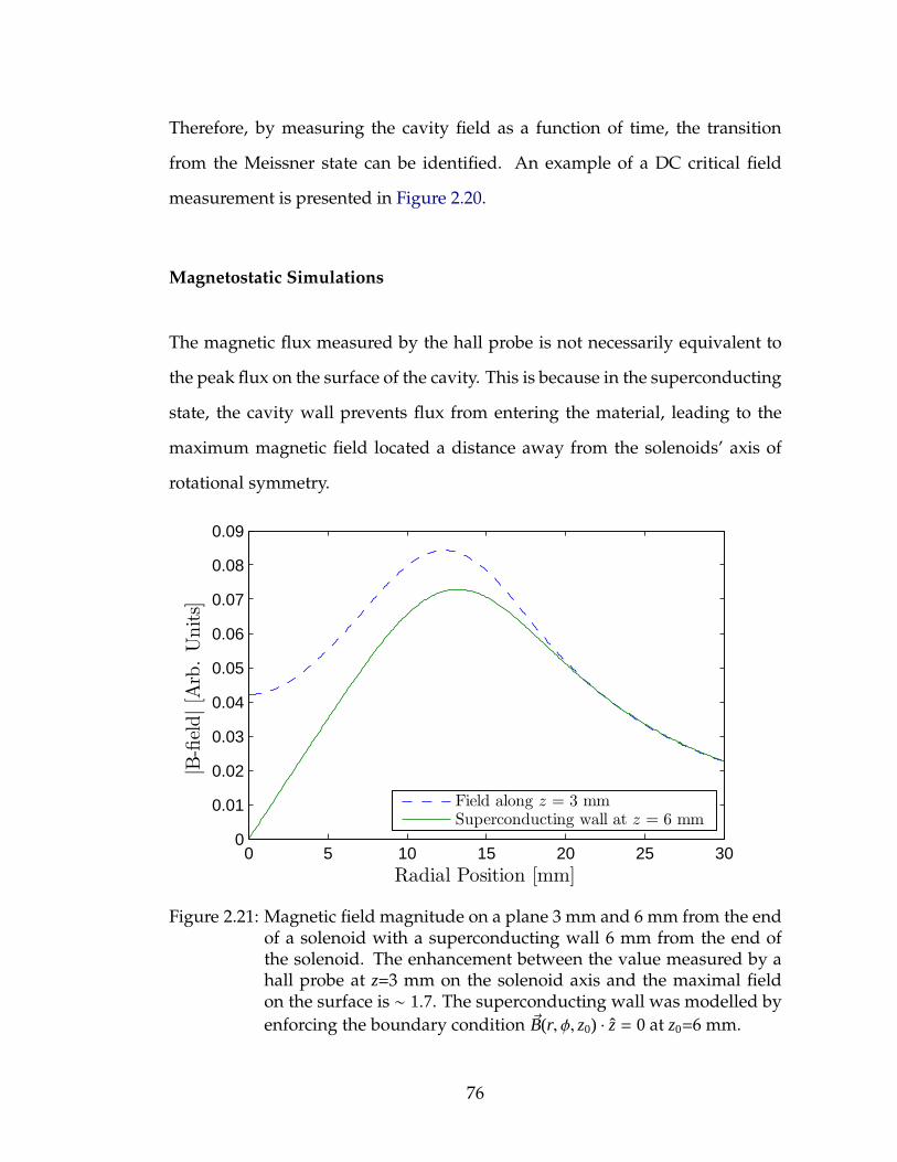
Therefore, by measuring the cavity field as a function of time, the transition
from the Meissner state can be identified. An example of a DC critical field
measurement is presented in Figure 2.20.
Magnetostatic Simulations
The magnetic flux measured by the hall probe is not necessarily equivalent to
the peak flux on the surface of the cavity. This is because in the superconducting
state, the cavity wall prevents flux from entering the material, leading to the
maximum magnetic field located a distance away from the solenoids’ axis of
rotational symmetry.
0 5 10 15 20 25 300
0.01
0.02
0.03
0.04
0.05
0.06
0.07
0.08
0.09
Radial Position [mm]
|B-fi
eld|[A
rb.
Units]
Field along z = 3 mmSuperconducting wall at z = 6 mm
Figure 2.21: Magnetic field magnitude on a plane 3 mm and 6 mm from the endof a solenoid with a superconducting wall 6 mm from the end ofthe solenoid. The enhancement between the value measured by ahall probe at z=3 mm on the solenoid axis and the maximal fieldon the surface is ∼ 1.7. The superconducting wall was modelled by
enforcing the boundary condition ~B(r, φ, z0) · z = 0 at z0=6 mm.
76
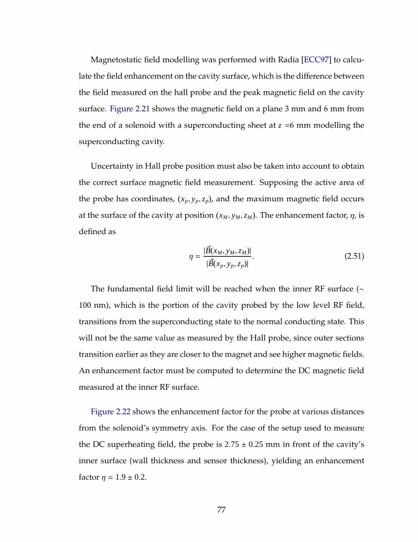
Magnetostatic field modelling was performed with Radia [ECC97] to calcu-
late the field enhancement on the cavity surface, which is the difference between
the field measured on the hall probe and the peak magnetic field on the cavity
surface. Figure 2.21 shows the magnetic field on a plane 3 mm and 6 mm from
the end of a solenoid with a superconducting sheet at z =6 mm modelling the
superconducting cavity.
Uncertainty in Hall probe position must also be taken into account to obtain
the correct surface magnetic field measurement. Supposing the active area of
the probe has coordinates, (xp, yp, zp), and the maximum magnetic field occurs
at the surface of the cavity at position (xM , yM, zM). The enhancement factor, η, is
defined as
η =|~B(xM , yM, zM)||~B(xp, yp, zp)|
. (2.51)
The fundamental field limit will be reached when the inner RF surface (∼
100 nm), which is the portion of the cavity probed by the low level RF field,
transitions from the superconducting state to the normal conducting state. This
will not be the same value as measured by the Hall probe, since outer sections
transition earlier as they are closer to the magnet and see higher magnetic fields.
An enhancement factor must be computed to determine the DC magnetic field
measured at the inner RF surface.
Figure 2.22 shows the enhancement factor for the probe at various distances
from the solenoid’s symmetry axis. For the case of the setup used to measure
the DC superheating field, the probe is 2.75± 0.25 mm in front of the cavity’s
inner surface (wall thickness and sensor thickness), yielding an enhancement
factor η = 1.9± 0.2.
77
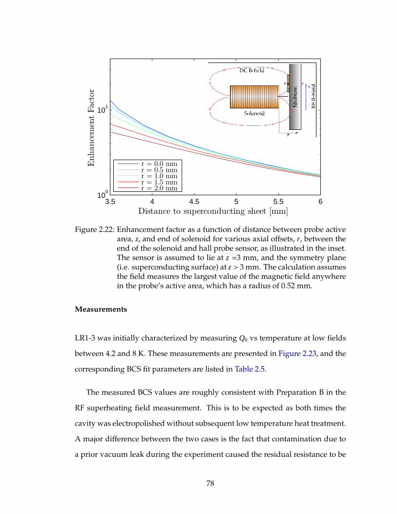
3.5 4 4.5 5 5.5 610
0
101
Distance to superconducting sheet [mm]
Enhance
men
tFact
or
r = 0.0 mmr = 0.5 mmr = 1.0 mmr = 1.5 mmr = 2.0 mm
Figure 2.22: Enhancement factor as a function of distance between probe activearea, z, and end of solenoid for various axial offsets, r, between theend of the solenoid and hall probe sensor, as illustrated in the inset.The sensor is assumed to lie at z =3 mm, and the symmetry plane(i.e. superconducting surface) at z > 3 mm. The calculation assumesthe field measures the largest value of the magnetic field anywherein the probe’s active area, which has a radius of 0.52 mm.
Measurements
LR1-3 was initially characterized by measuring Q0 vs temperature at low fields
between 4.2 and 8 K. These measurements are presented in Figure 2.23, and the
corresponding BCS fit parameters are listed in Table 2.5.
The measured BCS values are roughly consistent with Preparation B in the
RF superheating field measurement. This is to be expected as both times the
cavity was electropolished without subsequent low temperature heat treatment.
A major difference between the two cases is the fact that contamination due to
a prior vacuum leak during the experiment caused the residual resistance to be
78
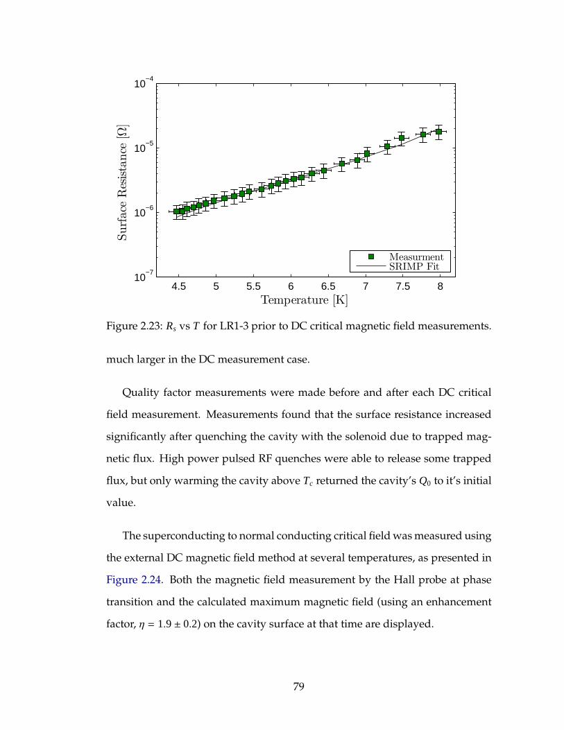
4.5 5 5.5 6 6.5 7 7.5 810
−7
10−6
10−5
10−4
Temperature [K]
Surf
ace
Res
ista
nce
[Ω]
MeasurmentSRIMP Fit
Figure 2.23: Rs vs T for LR1-3 prior to DC critical magnetic field measurements.
much larger in the DC measurement case.
Quality factor measurements were made before and after each DC critical
field measurement. Measurements found that the surface resistance increased
significantly after quenching the cavity with the solenoid due to trapped mag-
netic flux. High power pulsed RF quenches were able to release some trapped
flux, but only warming the cavity above Tc returned the cavity’s Q0 to it’s initial
value.
The superconducting to normal conducting critical field was measured using
the external DC magnetic field method at several temperatures, as presented in
Figure 2.24. Both the magnetic field measurement by the Hall probe at phase
transition and the calculated maximum magnetic field (using an enhancement
factor, η = 1.9± 0.2) on the cavity surface at that time are displayed.
79

Input Parameter Value UnitFrequency 1300 MHzTc 9.20 KλL 39.00 nmξ0 38.00 nmFit Parameter Value UnitEg 4.408 ± 0.052 —ℓtr 2.94× 10⁴ ± 1.77× 10⁴ nmR0 133. ± 14.0 nΩCalculated Result Value Unitλtr 0.001 ± 0.001 —R(λtr) 1.000 ± 0.001 —λGL 27.59 ± 0.01 nmξGL 28.05 ± 3× 10⁻⁴ nmκGL 0.98 ± 7× 10⁻⁴ —c(κGL) 1.26 ± 2× 10⁻⁴ —
Table 2.5: Material properties used to fit surface resistance vs temperature datapresented in Figure 2.23, with Eg, ℓtr and R0 as fit parameters. Thecritical temperature was measured separately. The small uncertaintyof the calculated parameters are due to the large mean free path.
Fitting the maximum surface B-field, as a function of t = T/Tc, with the phe-
nomenological prediction (assuming c(κGL) is temperature independent, which
is justified by the close fit to the data).
Bsh(t) = c(κGL) · Bc ·(
1− t2)
, (2.52)
where Bc = 200mT, [FSS66] yields the result c(κGL) = 1.216± 0.098.
The agreement between the values of c(κGL) obtained from the superheating
field measurements with the GL prediction using the material properties listed
in Table 2.5, argues that, as for the superheating field measurement using RF
fields, BDCmax,sc = Bsh, for κGL ∼ 1.
The DC field apparatus enabled measurement of Bsh without being lim-
ited by the RF heating of the inner wall. This result demonstrates that for
80
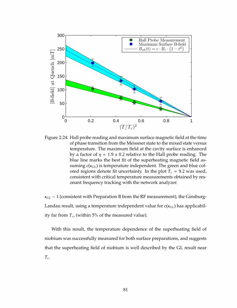
(T/Tc)2
|B-fi
eld|at
Quen
ch[m
T]
0 0.2 0.4 0.6 0.8 10
50
100
150
200
250
300Hall Probe MeasurementMaximum Surface B-fieldBsh(t) = c ·Bc ·
(
1− t2)
Figure 2.24: Hall probe reading and maximum surface magnetic field at the timeof phase transition from the Meissner state to the mixed state versustemperature. The maximum field at the cavity surface is enhancedby a factor of η = 1.9 ± 0.2 relative to the Hall probe reading. Theblue line marks the best fit of the superheating magnetic field as-suming c(κGL) is temperature independent. The green and blue col-ored regions denote fit uncertainty. In the plot Tc = 9.2 was used,consistent with critical temperature measurements obtained by res-onant frequency tracking with the network analyzer.
κGL ∼ 1 (consistent with Preparation B from the RF measurement), the Ginsburg-
Landau result, using a temperature independent value for c(κGL) has applicabil-
ity far from Tc, (within 5% of the measured value).
With this result, the temperature dependence of the superheating field of
niobium was successfully measured for both surface preparations, and suggests
that the superheating field of niobium is well described by the GL result near
Tc.
81
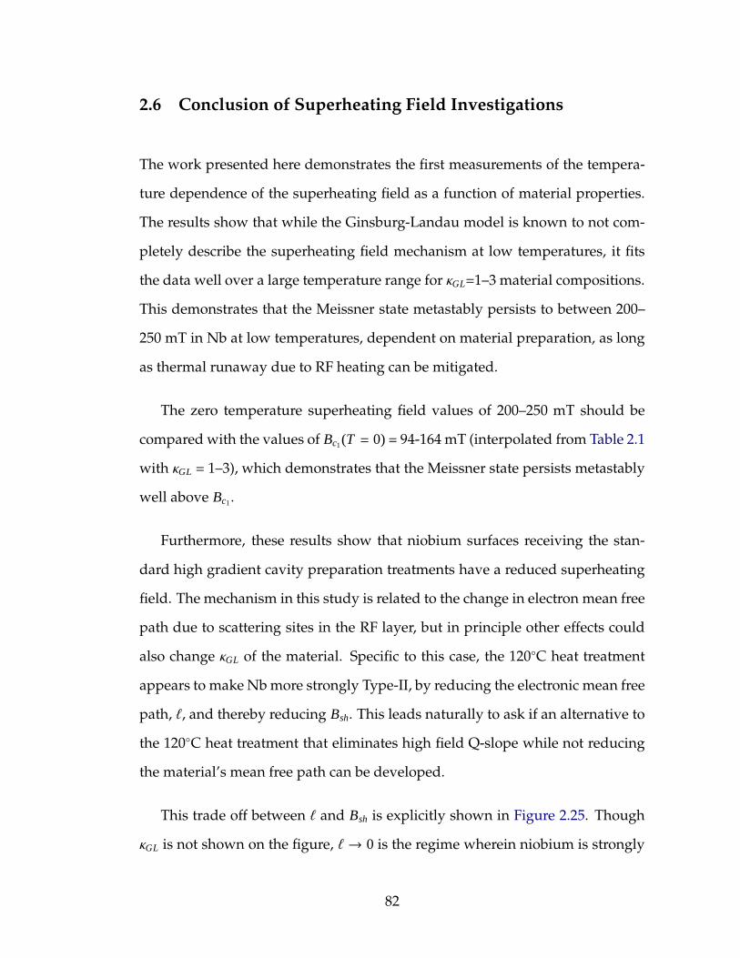
2.6 Conclusion of Superheating Field Investigations
The work presented here demonstrates the first measurements of the tempera-
ture dependence of the superheating field as a function of material properties.
The results show that while the Ginsburg-Landau model is known to not com-
pletely describe the superheating field mechanism at low temperatures, it fits
the data well over a large temperature range for κGL=1–3 material compositions.
This demonstrates that the Meissner state metastably persists to between 200–
250 mT in Nb at low temperatures, dependent on material preparation, as long
as thermal runaway due to RF heating can be mitigated.
The zero temperature superheating field values of 200–250 mT should be
compared with the values of Bc1(T = 0) = 94-164 mT (interpolated from Table 2.1
with κGL = 1–3), which demonstrates that the Meissner state persists metastably
well above Bc1.
Furthermore, these results show that niobium surfaces receiving the stan-
dard high gradient cavity preparation treatments have a reduced superheating
field. The mechanism in this study is related to the change in electron mean free
path due to scattering sites in the RF layer, but in principle other effects could
also change κGL of the material. Specific to this case, the 120C heat treatment
appears to make Nb more strongly Type-II, by reducing the electronic mean free
path, ℓ, and thereby reducing Bsh. This leads naturally to ask if an alternative to
the 120C heat treatment that eliminates high field Q-slope while not reducing
the material’s mean free path can be developed.
This trade off between ℓ and Bsh is explicitly shown in Figure 2.25. Though
κGL is not shown on the figure, ℓ → 0 is the regime wherein niobium is strongly
82
type-II, and ℓ → ∞ is the regime in which niobium is closer to type-I. The fact
that niobium’s material properties can drastically change depending on prepa-
ration should be carefully considered in SRF design of niobium accelerators.
10−1
100
101
102
103
120
140
160
180
200
220
240
260
Mean Free Path, ℓ [nm]
Bsh(T
)[m
T]
T = 0 KT = 1.6 KT = 2.0 KT = 4.2 K
Figure 2.25: Bsh for niobium vs ℓ at several temperatures computed by Bsh(t) =c(κGL) · 200 ·
[
1− t2]
, where t = T/Tc, and c(κGL) is the GL resultnear Tc. Clean niobium has ℓ → ∞, with a maximum superheatingfield of about 250 mT at zero temperature. The 120C heat treat-ment yields ℓ ∼10 nm, with a zero temperature superheating fieldof about 200 mT.
Theoretical progress on the temperature dependence of intermediate κGL ma-
terials are continuing with work on the Eilenberger equations, though there are
still questions about the convergence of these results at very low temperatures.
Thus, the work here provides much needed experimental data to help guide the
further development of theory.
A new type of experimental apparatus was developed to measure the super-
heating magnetic field of niobium with strong Q-slope preventing pulsed RF
83

measurements. The apparatus utilizes a superconducting solenoid, and mea-
surements demonstrated that the Ginsburg-Landau result for the superheating
field of niobium near Tc is applicable over a large temperature range.
We now return to the question that ignited these investigations: ”What is
the maximum gradient that can be supported in a niobium SRF accelerating
structure?” For typical high gradient accelerating structures, such as the TESLA
cavity geometry, the ratio of peak magnetic field to accelerating gradient is
4.26 mT/(MV/m), [ABB+00] meaning that at T=0 K, the largest gradient that can
be supported in a niobium cavity, assuming the high field Q-slope can be over-
come without the 120 heat treatment, is about 58.7 MV/m. With the heat treat-
ment, the accelerating gradient is limited to ∼47 MV/m. New cavity designs,
such as the Low Loss ILC cavity, with Bpk/Epk = 3.26 mT/(MV/m), [SKG+05]
may increase the maximal theoretical gradient to 69.2 MV/m, or 61 MV/m with
the 120 heat treatment.
Finally, the question of whether the superheating field results can be repro-
duced for alternative materials such as Nb3Sn or MgB2 is of central impor-
tance. Work is progressing rapidly on the production of Nb3Sn, [PL11] and
initial study of samples of this material are an active field of research, with
hints that this new material may allow the accelerating gradient to be dou-
bled. [Pos13b, CS08]
84
CHAPTER 3
MAIN LINAC CAVITY DESIGN FOR THE CORNELL ENERGY
RECOVERY LINAC
This chapter begins by introducing the idea behind an energy recovery linac
(ERL) and explains why it necessitates the use of superconducting accelerating
technology. Next, the phenomena of beam break-up is discussed, which is the
primary obstacle to the realization of a high current ERL, followed by the meth-
ods used to design the main linac accelerating structure. Finally, validation of
the design in 2D and 3D simulations are presented along with properties of the
final structure.
3.1 Energy Recovery Linac Principles
As discussed in section 1.4, progress on many frontiers of X-ray science require
very bright light sources with a large coherent fraction of the radiation. To this
end, Cornell University has developed a next generation light source, that is
brighter, and has a larger fraction of coherent X-rays than any existing storage
ring based light source (see Figure 3.1).
The spectral brightness of a photon source, B, is given by
B = F4π2ΣT
xΣTx′Σ
Ty Σ
Ty′, (3.1)
where F is the spectral flux1, and ΣTx,y are the photon source sizes in the trans-
verse directions and ΣTx′ ,y′ are their divergences. [BBB+11] Because the photon
1Flux is the rate at which electromagnetic energy is transferred through a surface, but inthe synchrotron light source community, only the fraction of photons near the maximum inthe intensity vs frequency function is considered yielding the units of spectral flux of [photon-s/s/0.1%BW].
85
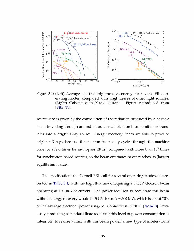
Figure 3.1: (Left) Average spectral brightness vs energy for several ERL op-erating modes, compared with brightnesses of other light sources.(Right) Coherence in X-ray sources. Figure reproduced from[BBB+11].
source size is given by the convolution of the radiation produced by a particle
beam travelling through an undulator, a small electron beam emittance trans-
lates into a bright X-ray source. Energy recovery linacs are able to produce
brighter X-rays, because the electron beam only cycles through the machine
once (or a few times for multi-pass ERLs), compared with more than 105 times
for synchrotron based sources, so the beam emittance never reaches its (larger)
equilibrium value.
The specifications the Cornell ERL call for several operating modes, as pre-
sented in Table 3.1, with the high flux mode requiring a 5 GeV electron beam
operating at 100 mA of current. The power required to accelerate this beam
without energy recovery would be 5 GV·100 mA = 500 MW, which is about 70%
of the average electrical power usage of Connecticut in 2011. [Adm13] Obvi-
ously, producing a standard linac requiring this level of power consumption is
infeasible; to realize a linac with this beam power, a new type of accelerator is
86
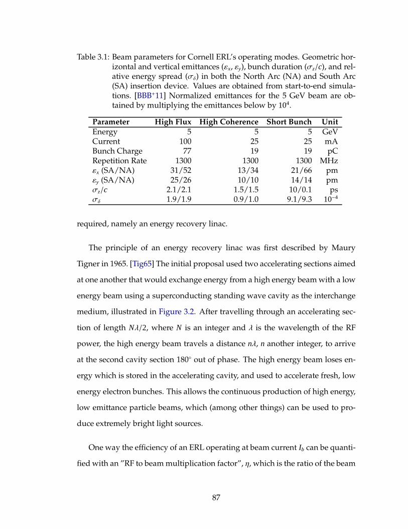
Table 3.1: Beam parameters for Cornell ERL’s operating modes. Geometric hor-izontal and vertical emittances (εx, εy), bunch duration (σz/c), and rel-ative energy spread (σδ) in both the North Arc (NA) and South Arc(SA) insertion device. Values are obtained from start-to-end simula-tions. [BBB+11] Normalized emittances for the 5 GeV beam are ob-tained by multiplying the emittances below by 104.
Parameter High Flux High Coherence Short Bunch Unit
Energy 5 5 5 GeVCurrent 100 25 25 mABunch Charge 77 19 19 pCRepetition Rate 1300 1300 1300 MHzεx (SA/NA) 31/52 13/34 21/66 pmεy (SA/NA) 25/26 10/10 14/14 pmσz/c 2.1/2.1 1.5/1.5 10/0.1 psσδ 1.9/1.9 0.9/1.0 9.1/9.3 10−4
required, namely an energy recovery linac.
The principle of an energy recovery linac was first described by Maury
Tigner in 1965. [Tig65] The initial proposal used two accelerating sections aimed
at one another that would exchange energy from a high energy beam with a low
energy beam using a superconducting standing wave cavity as the interchange
medium, illustrated in Figure 3.2. After travelling through an accelerating sec-
tion of length Nλ/2, where N is an integer and λ is the wavelength of the RF
power, the high energy beam travels a distance nλ, n another integer, to arrive
at the second cavity section 180 out of phase. The high energy beam loses en-
ergy which is stored in the accelerating cavity, and used to accelerate fresh, low
energy electron bunches. This allows the continuous production of high energy,
low emittance particle beams, which (among other things) can be used to pro-
duce extremely bright light sources.
One way the efficiency of an ERL operating at beam current Ib can be quanti-
fied with an ”RF to beam multiplication factor”, η, which is the ratio of the beam
87
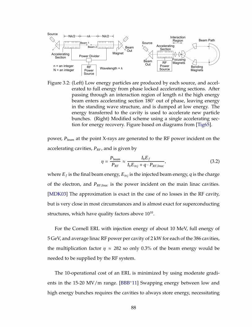
Figure 3.2: (Left) Low energy particles are produced by each source, and accel-erated to full energy from phase locked accelerating sections. Afterpassing through an interaction region of length nλ the high energybeam enters accelerating section 180 out of phase, leaving energyin the standing wave structure, and is dumped at low energy. Theenergy transferred to the cavity is used to accelerate new particlebunches. (Right) Modified scheme using a single accelerating sec-tion for energy recovery. Figure based on diagrams from [Tig65].
power, Pbeam at the point X-rays are generated to the RF power incident on the
accelerating cavities, PRF, and is given by
η =Pbeam
PRF≈
IbE f
IbEin j + q · PRF,linac, (3.2)
where E f is the final beam energy, Ein j is the injected beam energy, q is the charge
of the electron, and PRF,linac is the power incident on the main linac cavities.
[MDK03] The approximation is exact in the case of no losses in the RF cavity,
but is very close in most circumstances and is almost exact for superconducting
structures, which have quality factors above 1010.
For the Cornell ERL with injection energy of about 10 MeV, full energy of
5 GeV, and average linac RF power per cavity of 2 kW for each of the 386 cavities,
the multiplication factor η ≈ 282 so only 0.3% of the beam energy would be
needed to be supplied by the RF system.
The 10-operational cost of an ERL is minimized by using moderate gradi-
ents in the 15-20 MV/m range. [BBB+11] Swapping energy between low and
high energy bunches requires the cavities to always store energy, necessitating
88
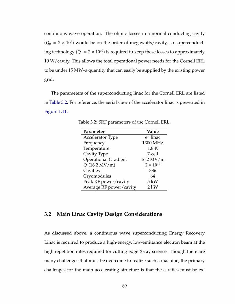
continuous wave operation. The ohmic losses in a normal conducting cavity
(Q0 ≈ 2 × 10⁴) would be on the order of megawatts/cavity, so superconduct-
ing technology (Q0 ≈ 2× 10¹⁰) is required to keep these losses to approximately
10 W/cavity. This allows the total operational power needs for the Cornell ERL
to be under 15 MW–a quantity that can easily be supplied by the existing power
grid.
The parameters of the superconducting linac for the Cornell ERL are listed
in Table 3.2. For reference, the aerial view of the accelerator linac is presented in
Figure 1.11.
Table 3.2: SRF parameters of the Cornell ERL.
Parameter Value
Accelerator Type e− linacFrequency 1300 MHzTemperature 1.8 KCavity Type 7-cellOperational Gradient 16.2 MV/mQ0(16.2 MV/m) 2× 10¹⁰
Cavities 386Cryomodules 64Peak RF power/cavity 5 kWAverage RF power/cavity 2 kW
3.2 Main Linac Cavity Design Considerations
As discussed above, a continuous wave superconducting Energy Recovery
Linac is required to produce a high-energy, low-emittance electron beam at the
high repetition rates required for cutting edge X-ray science. Though there are
many challenges that must be overcome to realize such a machine, the primary
challenges for the main accelerating structure is that the cavities must be ex-
89
tremely efficient, having Q0 > 2 × 10¹⁰ at 1.8 K, and the linac must be able to
support threshold current in excess of the 100 mA design specification while
preserving the small beam emittance created at the injector. The beam proper-
ties can be limited by the effect of strong higher-order modes (HOMs) in main
linac cavities. Thus, the accelerating structures comprising the main linac must
balance two opposing goals to achieve its science mission: obtain a very large
Q0 of the accelerating mode while making the Q0 of all HOMs very small.
Successful cavity design depends on maximizing the threshold current of a
very low emittance electron beam through the linac at the lowest cost. Since
cryogenic power expenses account for more than 50% of the electrical costs for
the ERL facility, it is important to examine the sources of power loss and their
scaling with machine parameters.
For a cryogenic cavity, power losses can be separated into static and dynamic
losses, both of which should be minimized for the ERL. The static losses are
due to heat transfer from radiation and conduction, and are minimized through
proper cryomodule design. Dynamic losses are due to the operation of the RF
structure.
Heat produced by an SRF cavity is absorbed by the cryogenic system. The
surface area of the cavity, and thus heat load per unit length scales inversely
with the fundamental mode frequency. This consideration motivates operation
at high frequencies.
The surface resistance of the cavity Rs has two contributions, the losses due
to BCS resistance, RBCS , and the residual resistance, R0. Following Equation 1.9,
90

the power dissipated in the linac, Pdiss per unit length, L, can be written as
Pdiss
L=
2π f UQ0L
, (3.3)
where U is the stored energy in the cavity operating at frequency f . Using Equa-
tion 1.11 and Equation 1.14, one finds that the power dissipated per unit length,
at a fixed voltage, depends on
Pdiss
L∝ RBCS + R0
f. (3.4)
Because RBCS increases with the square of the resonant frequency, low frequency
operation is favorable when this component of Rs is large. However, at low tem-
peratures the BCS component is negligible compared to the (roughly) frequency
independent residual resistance–typical values are between 5-10 nΩ–and favors
high frequency operation when this is the dominant factor. These considera-
tions lead to the conclusion that AC cooling power is minimized for frequencies
between 500 and 1500 MHz. [LK06]
An operating frequency of 1300 MHz was chosen for three main reasons:
First, the upper end of the frequency range has small cavity surface area, re-
ducing the chances of contamination during assembly. Second, higher frequen-
cies allow smaller electron bunch charges to be used for the same beam current,
which is important because smaller bunch charges help to mitigate space-charge
effects and allow smaller beam emittances. Third, much work has been done
developing 1300 MHz technology for the International Linear Collider and the
European XFEL, so using these mature technologies reduces research and devel-
opment costs by capitalizing on the availability of RF sources such as klystrons
and solid state amplifiers.
The number of cells for the cavity were chosen as a compromise between
maximizing linac fill factor, which increases with number of cells and reduces
91
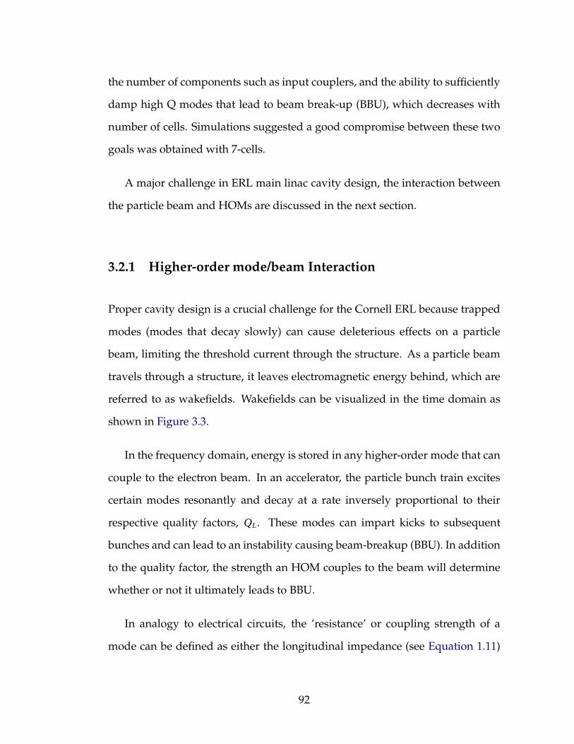
the number of components such as input couplers, and the ability to sufficiently
damp high Q modes that lead to beam break-up (BBU), which decreases with
number of cells. Simulations suggested a good compromise between these two
goals was obtained with 7-cells.
A major challenge in ERL main linac cavity design, the interaction between
the particle beam and HOMs are discussed in the next section.
3.2.1 Higher-order mode/beam Interaction
Proper cavity design is a crucial challenge for the Cornell ERL because trapped
modes (modes that decay slowly) can cause deleterious effects on a particle
beam, limiting the threshold current through the structure. As a particle beam
travels through a structure, it leaves electromagnetic energy behind, which are
referred to as wakefields. Wakefields can be visualized in the time domain as
shown in Figure 3.3.
In the frequency domain, energy is stored in any higher-order mode that can
couple to the electron beam. In an accelerator, the particle bunch train excites
certain modes resonantly and decay at a rate inversely proportional to their
respective quality factors, QL. These modes can impart kicks to subsequent
bunches and can lead to an instability causing beam-breakup (BBU). In addition
to the quality factor, the strength an HOM couples to the beam will determine
whether or not it ultimately leads to BBU.
In analogy to electrical circuits, the ’resistance’ or coupling strength of a
mode can be defined as either the longitudinal impedance (see Equation 1.11)
92
Figure 3.3: Wakefields from a 1.5 cm long bunch∗ as it traverses an acceleratingstructure. High intensity electric field is red and no field is blue.Calculation was performed using SLACs time domain solver T3P,[Xia97, KCG+10] running in parallel on 720 nodes at NERSC. [Nat]The full calculation took ∼1000 computer-hours.∗Bunch charge was 25 times larger than the 0.6 mm bunch that will be used in theERL, due to memory limitations.
for monopole modes or the transverse impedance in Equation 1.20 for non-
monopole modes,2 as was discussed in section 1.1.1. Non-monopole modes are
only excited by a beam travelling off-axis.
Following [Wie95], the effect of an HOM on a charge, q, travelling with rela-
tive velocity β = v/c can be calculated. The transverse variation of the longitu-
dinal field of a HOM, having transverse electric and magnetic fields E⊥ and B⊥,
2Non-monopole modes have zero field component along the axis so the voltage integral inEquation 1.7 vanishes.
93
imparts a transverse momentum kick
p⊥ =qβ
∫ [
E⊥ +1c
(v × B)⊥
]
dz. (3.5)
The transverse vector potential A⊥ can be used to write E⊥ = −∂tA⊥ and B =
(∇ × A)⊥ to yield
∂p∂t= −q
c∇⊥
∫
Ez dz, (3.6)
yielding the Panofsky-Wenzel theorem that was used to derive Equation 1.20,
[PW56] which relates a mode’s coupling strength to the transverse momentum
kick a particle bunch receives.
The interaction between higher-order modes and the electron beam are of
primary concern for ERL operation. Next, the effect of monopole, dipole and
quadrupole modes are investigated.
Monopole Effects
Monopole HOMs, having non-zero field components along the beam axis, have
the effect of introducing longitudinal instabilities into an ERL beam by changing
the bunch energy, as has been studied in [SH06]. The threshold current, Ith,long
before longitudinal effects lead to BBU in an ERL is given by
Ith,long =2E
ηtrωλ
(RQ
)
λQλ
, (3.7)
where E is the energy of the beam, tr is the return time around the loop for an
on-energy particle and η is the ’slip factor’. The slip factor relates the time offset
∆T of a particle with energy offset ∆E as
∆T = ηtr∆EE. (3.8)
94
The 6-dimensional ray tracing formalism, which relates an initial particle
position X(0) with its final position X(s) after passing through elements having
a transfer matrix, R, [Cha99] via
x(s)
x′(s)
y(s)
y′(s)
l(s)
∆P(s)/P0
︸ ︷︷ ︸
X(s)
=
r11 r12 r13 r14 0 r16
r21 r22 r23 r24 0 r26
r31 r32 r33 r34 0 r36
r41 r42 r43 r44 0 r46
r51 r52 r53 r54 1 r56
0 0 0 0 0 1
︸ ︷︷ ︸
R
·
x(0)
x′(0)
y(0)
y′(0)
l(0)
∆P(0)/P0
︸ ︷︷ ︸
X(0)
, (3.9)
demonstrated that longitudinal BBU primarily depends on the r56 element
which couples path length differences, l, with momentum deviations ∆P/P. As
long as |r56| < 10 m, longitudinal BBU is not a danger (r56 ≈ 0 for all ERL oper-
ating modes, and is less than 0.6 m at all points in the ERL lattice in operating
mode C). [BBB+11] Therefore, longitudinal threshold current can be mitigated
with proper optics design of the accelerator, and is not a cavity design concern.
This theoretical result was compared with particle tracking simulations of
the Cornell ERL lattice, performed with with BMAD, [Sag06] accounting for the
4 strongest monopole modes. Simulations agreed with theory, and predicted
that for a mode with f = 3857.63 MHz, QL = 13728and (R/Q) = 31 Ω, Ith,long ∼
8.6×10⁴ mA, in the case of an ERL consisting of a single cavity and single HOM.
Again, monopole BBU is not a danger for the Cornell ERL operating at 100 mA.
95

Dipole Effects
Dipole HOMs couple beam displacement and subsequent kick after one pass
through the ERL. Instead of leading to energy spread, dipoles introduce trans-
verse kicks to the bunch which can lead to beam loss at current substantially
smaller than in the longitudinal BBU case.
The basic mechanism of transverse BBU is that a dipole mode applies a trans-
verse kick to a beam, which then returns to the same cavity with transverse
offset, leading to beam oscillation. Since the longitudinal voltage depends on
offset (see Equation 1.18), the oscillating beam drives the mode more strongly,
leading to an exponential instability.
The transverse voltage of dipole modes depends on offset, in contrast to
monopole modes, whose longitudinal voltage does not depend on offset. This
difference implies that a transverse oscillation will not drive a monopole mode
unless the frequency of the HOM is a harmonic of the bunch repetition rate.
On the other hand, a dipole mode can be driven if its frequency is a harmonic
of the beam’s oscillation frequency. Since the mode itself causes the transverse
oscillation, it will automatically oscillate at the resonant frequency, which is why
it is possible to get transverse beam breakup at any HOM frequency.3
A model of a single loop ERL consisting of one cavity with a single HOM
3Transverse beam breakup is analogous to closing a feedback loop with negative gain, high-lighting the inherent instability of the system. There is dependence on the return phase, whichis why beam breakup equations depend on return time.
96
was investigated theoretically with the use of a transport matrix, T , defined as
x(s)
x′(s)
y(s)
y′(s)
=
T11 T12 T13 T14
T21 T22 T23 T24
T31 T32 T33 T34
T41 T42 T43 T44
︸ ︷︷ ︸
T
·
x(0)
x′(0)
y(0)
y′(0)
, (3.10)
to arrive at an analytic result for the threshold current. [HBS07]4 The result is
Ith,dipole = −2ω
q · (R/Q)⊥,λ · Qλωλ
1T ∗12 sinωλtr
, (3.11)
where q is the bunch charge and in this case (R/Q)⊥,λ has units Ω/m2,5 and T ∗12
depends on the polarization angle of the HOM, θλ, according to
T ∗12 = T12 cos2 θλ + (T14 + T32) sinθλ cosθλ + T34 sin2 θλ. (3.12)
Initial simulations of the Cornell ERL lattice demonstrated that Ith,dipole in a real-
istic ERL can be substantially lower than the 100 mA design current, depending
on assumptions about the HOM properties. [BH04] This is consistent with sim-
ulations and observations of BBU in the Jefferson Laboratory prototype ERL
beginning at under 10 mA for modes having QL > 106, (R/Q)′⊥ ∼ 30Ω. [TBD+05]
Achieving 100 mA current in the Cornell ERL requires an order of magnitude
reduction in dipole HOM strength and requires a very careful cavity design.
The realistic case of an ERL consisting of hundreds of cavities with many
unique modes per cavity must be treated with particle tracking simulations,
since coherent effects between cavities can introduce large corrections to the
4R/Q in this equation has been converted from the form presented in [BH04] to one consis-tent with later work in subsection 3.2.2.
5Various R/Q definitions having units of Ohms, Ohms/m, and Ohms/m2 can be convertedto one another by multiplication of k = ω/c, a point first brought to my attention by V. Yakolev.[Yak11]
97
single cavity result in Equation 3.11. Unlike the monopole BBU case, the lat-
tice optics properties can not always be adjusted to mitigate transverse dipole
effects, so special care must be taken in cavity design to eliminate the effects
of dipole HOMs that could limit Ith,dipole below the 100 mA design specification.
This will be discussed more thoroughly in subsection 3.2.2.
Quadrupole Effects
The effect of quadrupole modes leading to transverse BBU effects was explored
in [SH07]. The theory for quadrupole transverse kicks depends on the beta func-
tions6 of the accelerated and returning beam in the horizontal and vertical di-
rections, β1x, β2x, β1y, β2y, and the difference in betatron oscillations,7 ∆ψx,∆ψy,
caused by the quadrupole kick.
The analytic result of threshold current, Ith,quad , in an ERL consisting of a
single cavity with a single quadrupole mode is
Ith,quad = −Eωλ
qc
γr40
2(
RQ
)
λQλǫn
1(βx1βx2 sin 2∆ψx + βy1βy2 sin 2∆ψy)
1sinωλtr
, (3.13)
where E is the beam energy, γ is the Lorentz factor of the beam, ǫn is the nor-
malized emittance of the beam, and r0 is the distance perpendicular to the beam
axis at which (R/Q)λ8 is measured. [SH07] For reference, the beta functions of the
beams travelling through accelerating sections in the Cornell ERL are presented
in Figure 3.4. Simulations of a full linac with quadrupole HOMs having quality
factors of ∼ 109 yielded Ith,quad > 100mA for a 5 GeV electron beam, even in a full
6The beta function is related to the to the transverse size of the particle beam. [ES93]7Betatron oscillations are transverse oscillations exhibited by a particle offset from the on-
orbit path. [Wil00]8(R/Q)λ has units of Ohms.
98

Figure 3.4: Beta functions of the electron beam in both linacs in acceleration anddeceleration stages. The linac is broken into two portions. The initialand final energies at each stage of the linac is noted on each plot.Plots reproduced from [BBB+11].
ERL lattice where all cavities have the same resonant frequency.9 The threshold
current is several times higher than the 100 mA design specification for realistic
frequency spread, so quadrupole modes with QL ∼ 109 are acceptable. [BBB+11]
9This is an unrealistic, worst-case, assumption. Relative spread in the quadrupole modefrequency, which is virtually guaranteed from fabrication variation, would increase Ith,quad.
99
3.2.2 General Scaling Factors
The first step of any optimization relies on obtaining an appropriate goal func-
tion. For the design of the Cornell ERL main linac cavities, the goal function
must reflect the need to obtain a large threshold current, Ith, through the ERL,
and recognize that an analytic solution is not available. A single strong HOM
can cause beam breakup. Coherent effects between several strong HOMs can
reduce the threshold current even further. Thus, maximizing Ith, through the
accelerator before beam instability sets in is the primary objective of the opti-
mization.
Given many higher-order modes in hundreds of accelerating cavities form-
ing the linac, Ith can only accurately be determined by statistical particle track-
ing. Since particle tracking is an expensive calculation, we sought an analytic
parameterization of the threshold current that shares the same scaling proper-
ties of the more expensive calculation.
To determine scaling of this parameter, particle tracking was performed with
BMAD [Sag06] on the Cornell ERL lattice. [May09] Each cavity in the lattice was
defined as having a single higher-order mode. The HOM’s quality factor, Q,
R/Q,10 and frequency, f , (with an assumed relative cavity-to-cavity frequency
spread,11 σ f / f of 5× 10⁻³) was varied over range of values.12
Figure 3.5 presents the beam tracking results when an HOM’s frequency and
R/Q is varied. The plots demonstrate that Ith ∝ (R/Q)−1 and Ith ∝ f , [VL10a] over
10For a multipole of order m, BMAD uses R/Q units of Ω/m2m.11The frequency spread has the effect of placing HOMs at slightly different frequencies from
one cavity to another, as occurs in a realistic machine. BMAD uses a random Gaussian distribu-tion with a root-mean-squared value of σ f .
12This range of σ f / f is typical of variations introduced by fabrication differences.
100

1 2 3 4 5 6 7 8 9 10 11
x 109
10−1
100
HOM Frequency [Hz]
I th
[A]
BMAD SimulationIth ∝ f (0.995±0.046)
10−4
10−3
10−2
10−1
100
101
102
10−1
100
101
102
103
R/Q [Ω/cm2]
I th
[A]
BMAD SimulationIth ∝ (R/Q)(−0.989±0.021)
Figure 3.5: Scaling of the threshold current for the Cornell ERL lattice populatedwith cavities having a single HOM with nominal properties of f =1.7 GHz, R/Q = 5 Ω/cm2, Q = 104 and a cavity-to-cavity frequencyspread of 5× 10⁻³. Markers denote average current, upper/lower er-ror bar denotes the current achieved by the top/bottom 10% of sim-ulated ERLs. Dotted lines show the best fit power-law dependenceof each parameter on Ith with 95% certainty.
the entire simulated range, in agreement with Equation 3.11. The scaling of Ith
with quality factor is more complicated, since it depends on the cavity-to-cavity
relative frequency spread. [HB04]
101
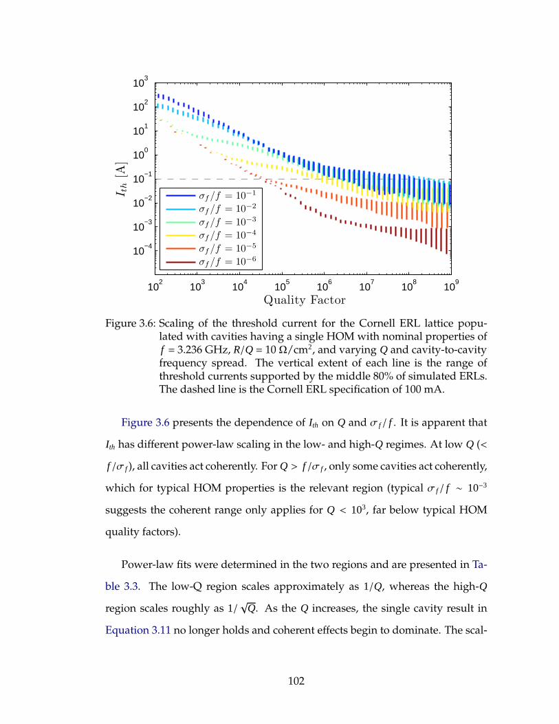
102
103
104
105
106
107
108
109
10−4
10−3
10−2
10−1
100
101
102
103
Quality Factor
I th
[A]
σf/f = 10−1
σf/f = 10−2
σf/f = 10−3
σf/f = 10−4
σf/f = 10−5
σf/f = 10−6
Figure 3.6: Scaling of the threshold current for the Cornell ERL lattice popu-lated with cavities having a single HOM with nominal properties off = 3.236 GHz, R/Q = 10 Ω/cm2, and varying Q and cavity-to-cavityfrequency spread. The vertical extent of each line is the range ofthreshold currents supported by the middle 80% of simulated ERLs.The dashed line is the Cornell ERL specification of 100 mA.
Figure 3.6 presents the dependence of Ith on Q and σ f / f . It is apparent that
Ith has different power-law scaling in the low- and high-Q regimes. At low Q (<
f /σ f ), all cavities act coherently. For Q > f /σ f , only some cavities act coherently,
which for typical HOM properties is the relevant region (typical σ f / f ∼ 10−3
suggests the coherent range only applies for Q < 103, far below typical HOM
quality factors).
Power-law fits were determined in the two regions and are presented in Ta-
ble 3.3. The low-Q region scales approximately as 1/Q, whereas the high-Q
region scales roughly as 1/√
Q. As the Q increases, the single cavity result in
Equation 3.11 no longer holds and coherent effects begin to dominate. The scal-
102
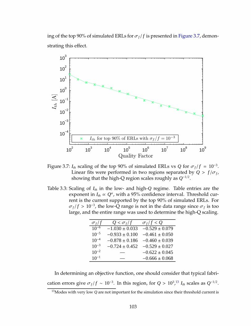
ing of the top 90% of simulated ERLs for σ f / f is presented in Figure 3.7, demon-
strating this effect.
102
103
104
105
106
107
108
109
10−4
10−3
10−2
10−1
100
101
102
103
Quality Factor
I th
[A]
Ith for top 90% of ERLs with σf/f = 10−3
Figure 3.7: Ith scaling of the top 90% of simulated ERLs vs Q for σ f / f = 10−3.Linear fits were performed in two regions separated by Q > f /σ f ,showing that the high-Q region scales roughly as Q−1/2.
Table 3.3: Scaling of Ith in the low- and high-Q regime. Table entries are theexponent in Ith ∝ Qα, with a 95% confidence interval. Threshold cur-rent is the current supported by the top 90% of simulated ERLs. Forσ f / f > 10−3, the low-Q range is not in the data range since σ f is toolarge, and the entire range was used to determine the high-Q scaling.
σ f / f Q < σ f/ f σ f / f < Q10−6 −1.030± 0.033 −0.529± 0.07910−5 −0.933± 0.100 −0.461± 0.05010−4 −0.878± 0.186 −0.460± 0.03910−3 −0.724± 0.452 −0.529± 0.02710−2 — −0.622± 0.04510−1 — −0.666± 0.068
In determining an objective function, one should consider that typical fabri-
cation errors give σ f / f ∼ 10−3. In this region, for Q > 103,13 Ith scales as Q−1/2.
13Modes with very low Q are not important for the simulation since their threshold current is
103
Taking the simulations into account, the threshold current for a given dipole
HOM, λ, in a realistic machine scales approximately as
Ith,λ ∝fλ
(R/Q)λ ·√
Qλ
. (3.14)
The objective function to be minimized then would be the worst HOM in the
structure, where worst is defined as having the largest value of
ξλ ≡(R/Q)λ ·
√Q
fλ. (3.15)
3.2.3 Geometric and electromagnetic constraints
Optimization constraints arise from physical manufacturing and preparation
concerns as well as features affecting accelerator performance. Geometrically,
cavity fabrication considerations limit the maximum radius of curvature in cell
to three times the sheet metal width. [Cho09] Niobium sheets pressed into cells
are 2 mm thick, requiring radii of curvature to be greater than 6 mm.
A standard cleaning procedure for preparing contaminant-free accelerating
structures is high-pressure rinsing. Drainage concerns require cavity wall slopes
of at least 5 from the horizontal to prevent water from pooling.
Electromagnetic considerations involve surface electric and magnetic fields
on the structure’s walls. The ratio of the peak surface electric field, Epk, to the
accelerating electric field, Eacc, should be kept to a low value to reduce the risk
of field-induced emission of electrons from dust particles on the cavity surface.
Field emission is particularly deleterious in CW operation since it can limit the
very large.
104
usable gradient by causing an additional cryogenic heat load and unacceptable
radiation levels. The decision was made to limit Epk/Eacc ≤ 2.1.14
Previous work has demonstrated that the cryogenic heat load (inversely pro-
portional to G · R/Q) is related to the ratio of the peak magnetic field, Bpk, to
the peak electric field. [She09a] Maintaining, Bpk/Eacc ≤ 4.2 was chosen to keep
dynamic losses within the operating capacity of the cryogenic plant, and is con-
sistent with a structure having a fundamental mode Q0 ≥ ×1010.
With the objective function and constraints defined, the next concern is solv-
ing the complex, multi-optimization problem as efficiently as possible.
3.3 Approach to Accelerating Structure Design
As discussed previously, strong HOM damping is required for beam stabil-
ity, and thus a major driver of the accelerating structure design. There are
many schemes to damp HOM power including antenna and waveguide cou-
plers that extract power, as well as beamline absorbers. [Mos89, CA99] The best
solution depends on beam parameters. Since the Cornell ERL requires very
strong broadband damping–extracting about 200 W of monopole power/cav-
ity, assuming no monopole modes are driven resonantly [BBB+11]–the follow-
ing damping scheme has been selected:
HOMs are absorbed in beamline dampers placed at either end of the cavity
at an intermediate temperature (∼ 80 K), as illustrated in Figure 3.8. The beam
pipes have a diameter such that all monopole and dipole HOMs are above the
14This number is similar to ILC cavities, and is about as low as possible for a cavity iris radiusof 35 mm. [She09a]
105
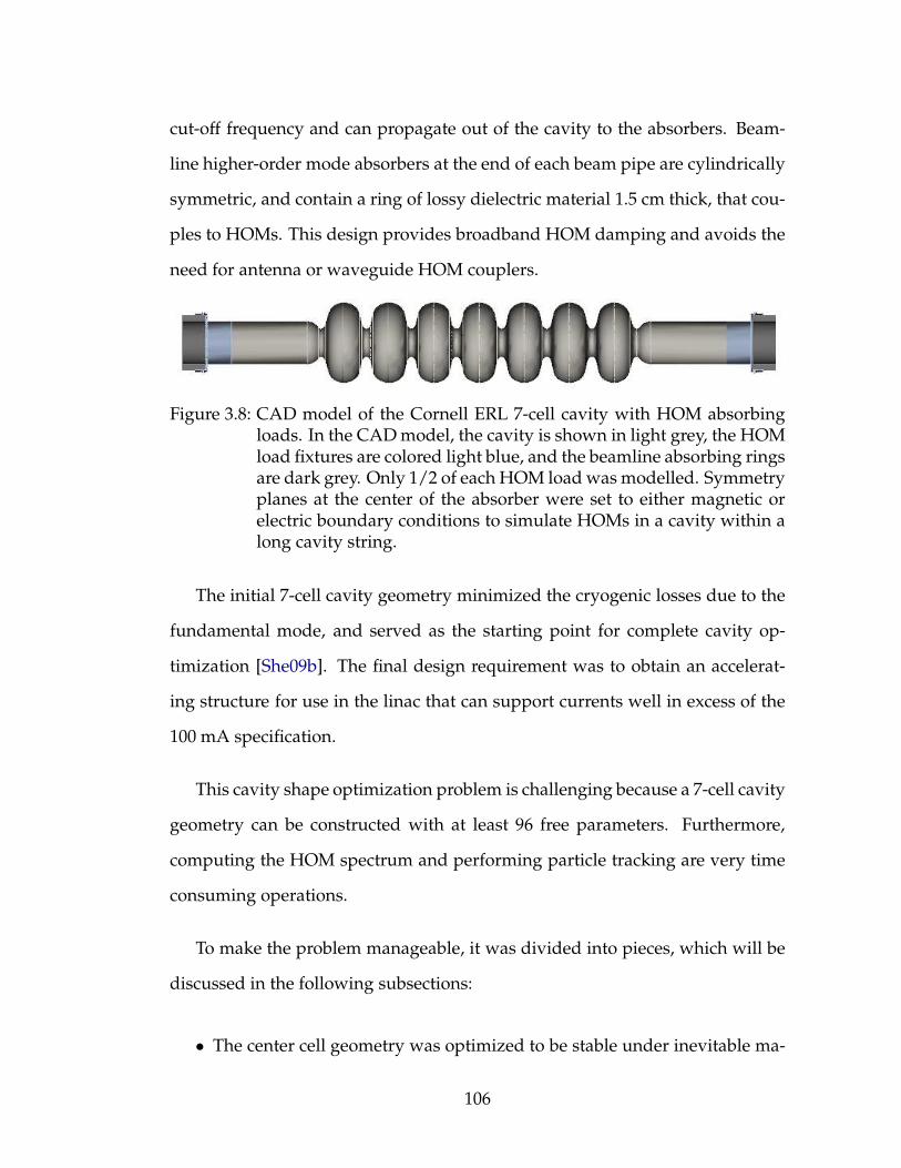
cut-off frequency and can propagate out of the cavity to the absorbers. Beam-
line higher-order mode absorbers at the end of each beam pipe are cylindrically
symmetric, and contain a ring of lossy dielectric material 1.5 cm thick, that cou-
ples to HOMs. This design provides broadband HOM damping and avoids the
need for antenna or waveguide HOM couplers.
Figure 3.8: CAD model of the Cornell ERL 7-cell cavity with HOM absorbingloads. In the CAD model, the cavity is shown in light grey, the HOMload fixtures are colored light blue, and the beamline absorbing ringsare dark grey. Only 1/2 of each HOM load was modelled. Symmetryplanes at the center of the absorber were set to either magnetic orelectric boundary conditions to simulate HOMs in a cavity within along cavity string.
The initial 7-cell cavity geometry minimized the cryogenic losses due to the
fundamental mode, and served as the starting point for complete cavity op-
timization [She09b]. The final design requirement was to obtain an accelerat-
ing structure for use in the linac that can support currents well in excess of the
100 mA specification.
This cavity shape optimization problem is challenging because a 7-cell cavity
geometry can be constructed with at least 96 free parameters. Furthermore,
computing the HOM spectrum and performing particle tracking are very time
consuming operations.
To make the problem manageable, it was divided into pieces, which will be
discussed in the following subsections:
• The center cell geometry was optimized to be stable under inevitable ma-
106

chining perturbations, while still maintaining low cryogenic losses due to
the fundamental mode.
• End cells were optimized to effectively couple HOMs to the absorbers.
• The solution was verified by performing particle tracking in an ERL con-
structed of realistic cavities with small shape imperfections.
Center Cell Design
The center cells of an elliptical shaped, β = 1 cavity are responsible for both the
properties of the fundamental accelerating mode and the dispersion relations of
the higher-order mode passbands. They are shaped by two ellipses connected
by a tangent line (see Figure 3.9) and can be described by 8 parameters. Only
6 parameters are free, since the length must be fixed to half a wavelength of
the RF frequency to synchronize relativistic particles, and one parameter must
be used to tune the cavity to the desired frequency. It is possible to generate
cell geometries that have very similar fundamental mode properties–resonant
frequency, geometry factor, G, R/Q, peak field ratios Epk/Eacc and Hpk/Eacc–while
having very different higher-order mode characteristics.
The initial center cell design minimized dynamic cryogenic losses due to the
fundamental mode, which is equivalent to minimizing the power lost in cavity
walls, Pc, at a given stored field energy, U, which is proportional to square of
the operating voltage, Vc. If the cavity has a the geometry factor, G, defined as
G = Q0 · Rs =ωµ0
∫
Ω|B|2 dΩ
∫
S|B|2 dS
, (1.14 revisited)
where the top integral is performed over the cavity volume, Ω, with a bounding
surface, S , and Rs is the average surface resistance of the cavity, the dissipated
107
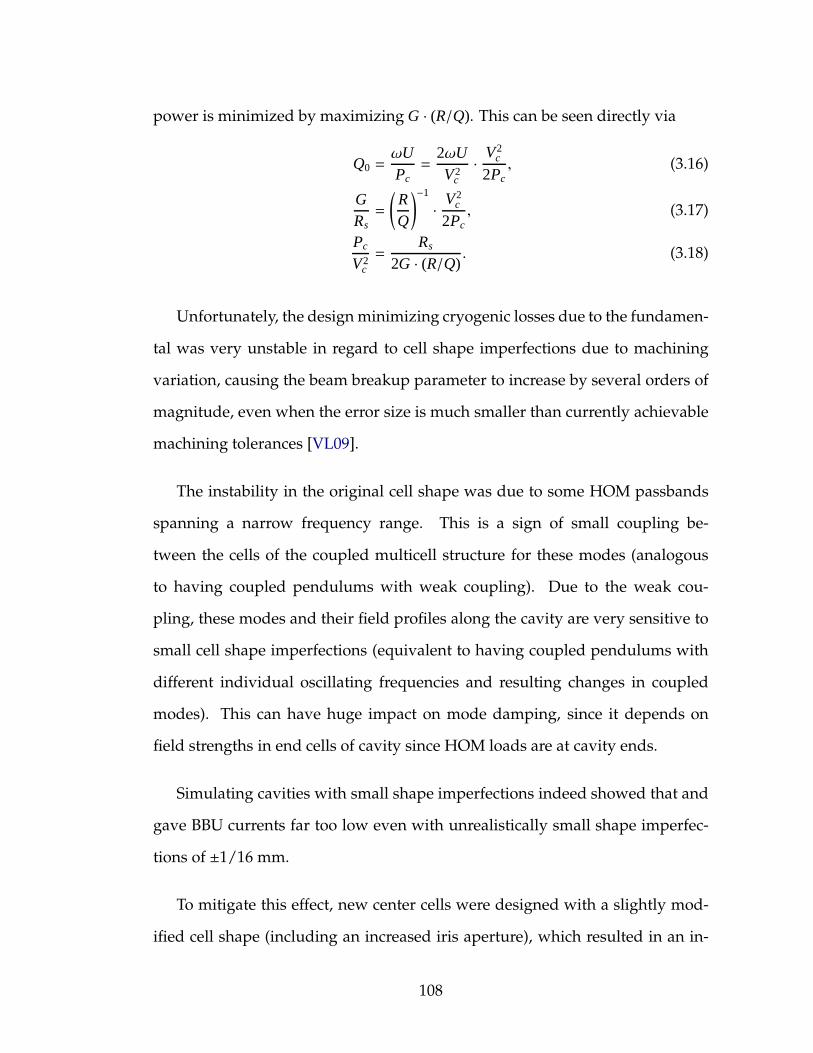
power is minimized by maximizing G · (R/Q). This can be seen directly via
Q0 =ωUPc=
2ωUV2
c
· V2c
2Pc, (3.16)
GRs=
(
RQ
)−1
· V2c
2Pc, (3.17)
Pc
V2c
=Rs
2G · (R/Q). (3.18)
Unfortunately, the design minimizing cryogenic losses due to the fundamen-
tal was very unstable in regard to cell shape imperfections due to machining
variation, causing the beam breakup parameter to increase by several orders of
magnitude, even when the error size is much smaller than currently achievable
machining tolerances [VL09].
The instability in the original cell shape was due to some HOM passbands
spanning a narrow frequency range. This is a sign of small coupling be-
tween the cells of the coupled multicell structure for these modes (analogous
to having coupled pendulums with weak coupling). Due to the weak cou-
pling, these modes and their field profiles along the cavity are very sensitive to
small cell shape imperfections (equivalent to having coupled pendulums with
different individual oscillating frequencies and resulting changes in coupled
modes). This can have huge impact on mode damping, since it depends on
field strengths in end cells of cavity since HOM loads are at cavity ends.
Simulating cavities with small shape imperfections indeed showed that and
gave BBU currents far too low even with unrealistically small shape imperfec-
tions of ±1/16 mm.
To mitigate this effect, new center cells were designed with a slightly mod-
ified cell shape (including an increased iris aperture), which resulted in an in-
108

creased width of the initially narrow higher-order mode passbands, while pre-
serving the properties of the fundamental mode’s R/Q ·G to within 5%. Increas-
ing the passband width and cell-to-cell coupling makes the field distribution
of the HOMs in a multicell cavity less sensitive to small dimensional varia-
tions. [VL09] This is accomplished by choosing cell geometries which have a
large frequency spread between the passband’s 0-mode, and the π-mode, as il-
lustrated in Figure 3.9.
Figure 3.9: From left to right, center cell geometry, lowest mode in a passbandhaving zero phase difference between cells, and the highest modein a passband with π-phase difference between the cells. Vectors areelectric field lines and colors correspond to electric field magnitude
The width of the first few HOM passbands are presented in Table 3.4. The
geometrical properties of the final center cell shape are presented with the full
optimization results in section 3.3.
Simulations demonstrated that cavities with the modified cavities were
much more robust in regard to machining variation and that realistic cell im-
perfections ( 0.5 mm) did not lead to strong changes in the HOM damping and
thus decrease the BBU current.
109

Table 3.4: Comparison of the frequency difference, ∆ f , between the 0-mode andπ-mode of several higher-order mode passbands between the originalcenter cell design and modified design. Notice the significantly in-creased width of the 3rd and 6th passband in the modified center cellshape.
Passband Original ∆ f Modified ∆ f[GHz] [MHz] [MHz]
1.8 192 1881.9 95 732.5 31 1072.7 277 2773.1 55 473.4 10 20
Table 3.5: Initial and final center cell geometric figures of merit. Cyrogeniclosses are slightly increased. The geometry factor and Epk/Eacc arefor the fundamental mode. Key: Eq.=Equator, Horiz.=Horizontal,Vert.=Vertical. The last four dimensions are half-axes of ellipses, mea-sured in cm. Table reproduced from [VL09].
Parameter Initial Optimized Unit
R/Q ·G 15576 14837 Ω2
Epk/Eacc 2.00 2.06 —Wall angle 85 77 DegreeIris Radius 3.500 3.598 cmEq. Horiz. 4.399 4.135 cmEq. Vert. 3.506 3.557 cmIris Horiz. 1.253 1.235 cmIris Vert. 2.095 2.114 cm
The center cell geometry found a good compromise between maximizing
R/Q ·G for the fundamental mode and reducing sensitivity to cell shape errors.
The center cells control the general features of the higher-order mode spec-
trum, so the next part of the design process is to ensure that the end cells effi-
ciently couple HOMs to the absorbers where their energy can be extracted.
110
End-cell Optimization
As mentioned above, the half-end cells couple the higher-order modes to the
beam line absorbers, thereby directly controlling HOM quality factors.
The end cell design includes a transition to a large beam pipe diameter
(110 mm) that allows all higher-order monopole and dipole modes to propa-
gate out of the cavity toward the beam pipe absorber. The two end cells are
asymmetric, which helps to prevent trapped modes by breaking symmetry and
shifting modes toward one end or the other. [Sek12] An iris reduction between
the end cell and beam tubes (see Figure 3.8)helps to maintain a large R/Q, while
the large beam pipe still allows HOMs to propagate out of the structure, a tech-
nique successfully employed in other designs [SBG+03, Mit91].
Each end cell geometry consist of an inner-half cell identical to the center cell
shape, and modified design of the outer half cell. It was parameterized by six
free variables per side. The end cell geometry is formed of two ellipses having
four parameters each (ellipse centers and half-axes), and two more ellipses form
an iris constriction flanging out to the beam pipe. Smoothness requirements
constrain one ellipses’ end points, as well as it’s tangent.
The optimizer varied the half-axes of the three ellipses denoted by the sym-
bols , , and in Figure 3.16. The vertical position of the ellipse whose center
is denoted by was also varied, adding a degree of freedom, but tuning re-
quirements limited constrained a degree of freedom yielding six total.
Physical requirements yield system constraints: (1) The cavity frequency
must be 1300 MHz, (2) The cryogenic losses due to the fundamental mode must
be maintained to within 5% of the baseline design, (3) Epk/Eacc < 2.1, which
111
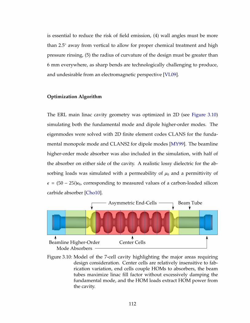
is essential to reduce the risk of field emission, (4) wall angles must be more
than 2.5 away from vertical to allow for proper chemical treatment and high
pressure rinsing, (5) the radius of curvature of the design must be greater than
6 mm everywhere, as sharp bends are technologically challenging to produce,
and undesirable from an electromagnetic perspective [VL09].
Optimization Algorithm
The ERL main linac cavity geometry was optimized in 2D (see Figure 3.10)
simulating both the fundamental mode and dipole higher-order modes. The
eigenmodes were solved with 2D finite element codes CLANS for the funda-
mental monopole mode and CLANS2 for dipole modes [MY99]. The beamline
higher-order mode absorber was also included in the simulation, with half of
the absorber on either side of the cavity. A realistic lossy dielectric for the ab-
sorbing loads was simulated with a permeability of µ0 and a permittivity of
ǫ = (50− 25i)ǫ0, corresponding to measured values of a carbon-loaded silicon
carbide absorber [Cho10].
Figure 3.10: Model of the 7-cell cavity highlighting the major areas requiringdesign consideration. Center cells are relatively insensitive to fab-rication variation, end cells couple HOMs to absorbers, the beamtubes maximize linac fill factor without excessively damping thefundamental mode, and the HOM loads extract HOM power fromthe cavity.
112
Each HOM passband was calculated using the four possible combinations of
electric and magnetic boundary conditions at the symmetry plane of the HOM
loads to simulate an infinitely long chain of identical cavities. This is more re-
alistic than open boundary conditions because open boundary conditions are
only applicable in the case of an isolated cavity, not one in a long chain of cav-
ities. Thus, the HOMs computed here much more accurately reflect what one
could expect in the main linac made out of a large number of cavities.
The optimization routine minimized the worst BBU parameter, ξλ, as defined
in (Equation 3.15) for dipole HOMs from 1.5–10.0 GHz, which for the 4 bound-
ary conditions meant computing the figures of merit for 1692 HOMs per itera-
tion [VL10b]. The optimization is challenging because geometry changes that
reduce the strength of one HOM can drastically increase the strength of another
HOM. Thus, the problem is to find end cell shapes that simultaneously min-
imizes the highest BBU parameters of all the HOMs, which is an intrinsically
non-analytic problem.
To simplify the optimization, the simultaneous minimization of N-HOMs
was treated as the analytic problem of minimizing the worst HOM, under the
non-analytic constraint that each BBU parameter of all other dipole modes in
the spectrum be less than the maximal BBU parameter of all the modes ≡ M.15
Minimization improves the BBU parameter by controlling the worst mode; all
other modes are required to fall below M for the point to be in the search space.
This process effectively minimizes all the HOMs simultaneously. Furthermore,
should the control HOM be below another mode that had a smaller value earlier
in the optimization, the optimization switches to control the new mode. Thus
the non-analytic problem is decomposed into an analytic problem with a non-
15Personal communication with J. Sethna
113
analytic constraint.
The constrained optimization was carried out in parallel on 256 processors16
with a simplex algorithm. MatLab code containing the basic structure of the
objective function is presented below.
1 func t ion worst RQQf = Corne l l ERL Ca vi ty Objec t ive Funct ion ( y )2 % Objec t ive funct ion f o r end c e l l opt imiz a t ion3
4 k i l l f l a g = 0 ; % S et to 1 i f a t e s t f a i l s5
6 % S c a l e the parameters to e l i m i n a t e the i n t e r v a l c o n s t r a i n t s7 % Get i n i t i a l input from d e s i r e ’ r e a l coord ina te guess ’ , x , transform8 % i n i t i a l i n p u t = atanh ( 2 . / ( p2−p1 ) . ∗ ( x−p1 ) −1)9 p1 = 1 . 0∗ ones ( s i z e ( y ) ) ; % Default min params
10 p2 = 4 . 5∗ ones ( s i z e ( y ) ) ; % Default max params11 x = ( p2 − p1 ) . ∗ ( tanh ( y ) + 1 ) /2 + p1 ;12
13 % Load run s e t t i n g s inc luding :14 % P r e f i x f o r geometry f i l e s15 % Which passbands to c a l c u l a t e16 % Number of modes to c a l c u l a t e/passband17 [ pre f ix , pass bands , modes ] = . . .18 C o r n e l l E R L C a v i t y r e a d r u n s e t t i n g s ( ’ ./ r u n s e t t i n g s . t x t ’ ) ;19
20 % # of passbands to c a l c u l a t e as well as # of boundary condi t ions21 num passbands = length ( pass bands ) ;22 bcs = 4 ;23
24 % Check i f end− c e l l parameters generate a s u i t a b l e geometry :25 % Curvature c o n s t r a i n t s must f a l l within s u i t a b l e l i m i t s26 % Cavity geometry must be tunable to 1300 MHz27 % Peak e l e c t r i c and magnetic f i e l d s must be within l i m i t s28 % Cavity q u a l i t y f a c t o r must be above 2 e1029 %30 % I f point i s unsuitable , s e t ’ k i l l f l a g ’ to 1 and re turn penalty31 % Else , re turn c a v i t y geometry and tune spacing32 [ k i l l f l a g , penalty , geo , s p l f , s p r t ] = . . .33 Cornell ERL Cavity check params ( y ) ;34
35 i f k i l l f l a g36 worst RQQf = penalty ;37 re turn38 end39
40 % Write f i l e s so the EM s o l v e r can compute HOMs41 Cornell ERL Cavity gen CLANS2 files ( . . .42 geo , pre f ix , num passbands , bcs ) ;
16Resources leased from Cornell’s Center for Advanced Computing
114

43
44 % Submit HOM j o b s to c l u s t e r .45 dos ( ’ python s u b m i t c l a n s 2 j o b s . py ’ ) ;46
47 % Wait f o r j o b s to complete and e x t r a c t data48 % I f too many f a i l to complete , a ss ign run a penalty value49 [ f , QL, R Q , k i l l f l a g , penalty ] = get HOM properties ( ) ;50
51 i f k i l l f l a g52 worst RQQF = penalty53 re turn54 end55
56 r e s u l t s v e c = [ f QL R Q ] ;57 rqqfs = R Q .∗ s q r t ( abs (QL) ) . / ( f r e q s ) ;58 f u l l v a l s = [ f reqs ’ , QL’ , R Q ’ , rqqfs ’ ] ;59
60 % Return the worst HOM f o r the mode in quest ion61 % I f another mode becomes 25% stronger , c o n t r o l on t h a t one ins tea d62 % B a s e l i n e metr ic i s max(R Q∗QL./ f )63 worst RQQf = Cornel l ERL Cavity control mode ( R Q , QL, f ) ;64
65 % Save r e s u l t s in a f o l d e r with the current time66 c a c h e f o l d e r = d a t e s t r (now , 3 0 ) ;67 save ( [ c a c h e f o l d e r ’ param . t x t ’ ] , . . .68 ’yp ’ , ’ xp ’ , ’ s p l f ’ , ’ s p r t ’ , ’−ASCII ’ ) ;69 save ( [ c a c h e f o l d e r ’ HOM results . t x t ’ ] , . . .70 ’ r e s u l t s v e c ’ , ’−ASCII ’ ) ;71 save ( [ c a c h e f o l d e r ’ f r e q s . t x t ’ ] , . . .72 ’ f r e q v e c ’ , ’−ASCII ’ ) ;73
74 h = semilogy ( f reqs , rqqfs , ’ b . ’ ) ;75 x l a b e l ( ’ Frequency [MHz] ’ ) ;76 y l a b e l ( ’ (R/Q) QLˆ1/2 f ˆ−1 [\Omega/cmˆ2/MHz] ’ ) ;77 grid on ;78 save ( [ f o l d e r ’ f u l l d a t a . t x t ’ ] , ’ f u l l v a l s ’ , ’−ASCII ’ ) ;79 saveas ( h , [ c a c h e f o l d e r ’ modeplot . f i g ’ ] ) ;80 saveas ( h , [ c a c h e f o l d e r ’ modeplot . png ’ ] ) ;81 end
The function Cornell_ERL_Cavity_check_params ensures that the ge-
ometry satisfies the constraint equations gi ≤ 0, and returns a penalty value in
the case that constraints are broken. Following [Rao09], the penalty function, p,
is assigned via
p = ξ∗ +∑
i
ai ·max(0, gi)2, (3.19)
115
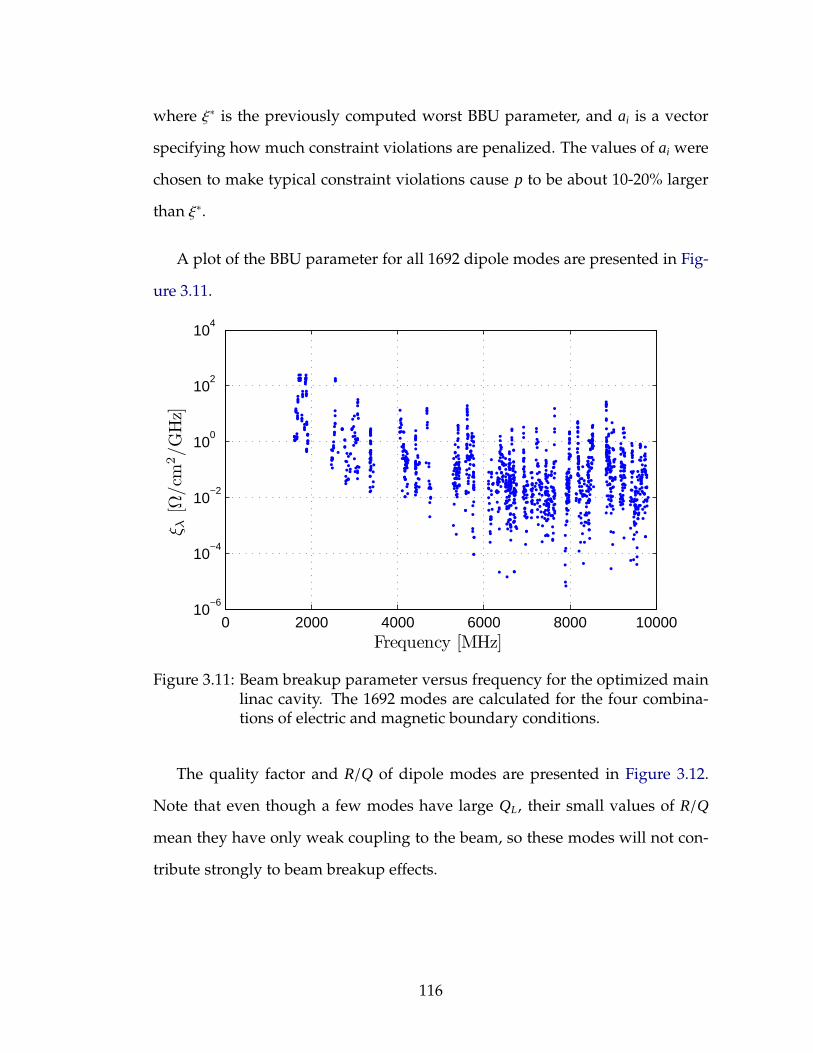
where ξ∗ is the previously computed worst BBU parameter, and ai is a vector
specifying how much constraint violations are penalized. The values of ai were
chosen to make typical constraint violations cause p to be about 10-20% larger
than ξ∗.
A plot of the BBU parameter for all 1692 dipole modes are presented in Fig-
ure 3.11.
0 2000 4000 6000 8000 1000010
−6
10−4
10−2
100
102
104
Frequency [MHz]
ξ λ[Ω
/cm
2/G
Hz]
Figure 3.11: Beam breakup parameter versus frequency for the optimized mainlinac cavity. The 1692 modes are calculated for the four combina-tions of electric and magnetic boundary conditions.
The quality factor and R/Q of dipole modes are presented in Figure 3.12.
Note that even though a few modes have large QL, their small values of R/Q
mean they have only weak coupling to the beam, so these modes will not con-
tribute strongly to beam breakup effects.
116
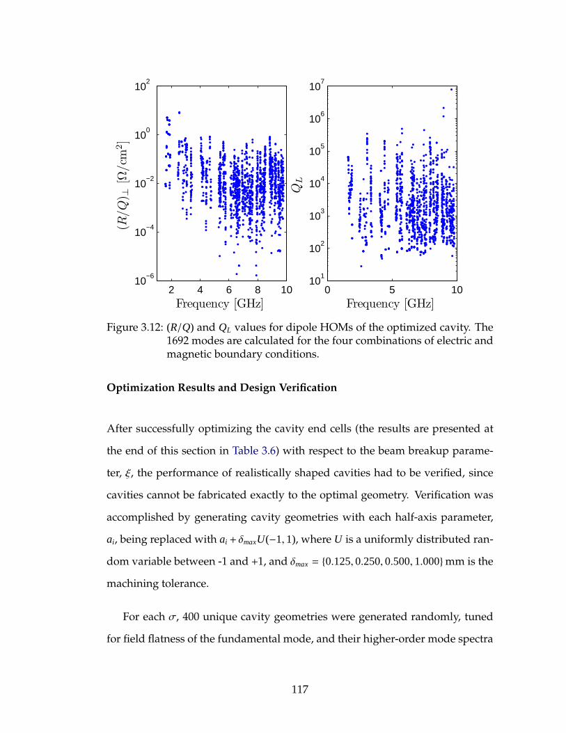
2 4 6 8 1010
−6
10−4
10−2
100
102
(R/Q
) ⊥[Ω
/cm
2]
Frequency [GHz]0 5 10
101
102
103
104
105
106
107
QL
Frequency [GHz]
Figure 3.12: (R/Q) and QL values for dipole HOMs of the optimized cavity. The1692 modes are calculated for the four combinations of electric andmagnetic boundary conditions.
Optimization Results and Design Verification
After successfully optimizing the cavity end cells (the results are presented at
the end of this section in Table 3.6) with respect to the beam breakup parame-
ter, ξ, the performance of realistically shaped cavities had to be verified, since
cavities cannot be fabricated exactly to the optimal geometry. Verification was
accomplished by generating cavity geometries with each half-axis parameter,
ai, being replaced with ai + δmaxU(−1, 1), where U is a uniformly distributed ran-
dom variable between -1 and +1, and δmax = 0.125, 0.250, 0.500, 1.000mm is the
machining tolerance.
For each σ, 400 unique cavity geometries were generated randomly, tuned
for field flatness of the fundamental mode, and their higher-order mode spectra
117

0
100
200
Counts
±1/8
mm
0
200
400
0
100
200
Counts
±1/2
mm
0
200
400
0
100
200
Counts
±1/2
mm
0
200
400
0 0.5 10
100
200
max(ξλ) [Ω/cm2/MHz]
Counts
±1
mm
1500 2000 2500 3000 35000
50
100
Frequency of max(ξλ) [MHz]
Figure 3.13: Histograms of the worst beam breakup parameters ξλ and the cor-responding frequencies for randomly generated cavities with var-ious machining tolerances. Each row contains data for a singlemachining tolerance. As the fabrication tolerances, δmax, loosen,maxξλ increases and the frequency of the strongest mode in the ERLstrays from the value it has in the ideal cavity. For larger tolerances,modes outside of the 2.5 GHz dipole passband begin to cause beambreakup.
were computed with CLANS2 (see Figure 3.13).
From this set of cavities, 100 ERLs were generated and simulated via particle
tracking to determine the BBU current. Each cavity location in the simulated
ERL lattice was populated with HOM properties (frequency, Q, and R/Q) from
a randomly selected cavity (drawn without replacement) with realistic shape
variations. The threshold current for each ERL was then computed with BMAD,
and the results are displayed in Figure 3.14. [VKL11]
118
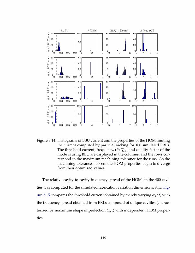
0 0.3 0.6 0.90
20
40
60Ith [A]
#(±
0.1
25
mm
)
1 2 30
50
100f [GHz]
0 5 100
10
20
30(R/Q)⊥ [Ω/cm2]
2 4 6 80
20
40
60Q [log10(Q)]
0 0.3 0.6 0.90
20
40
60
#(±
0.2
50
mm
)
1 2 30
20
40
60
0 5 100
5
10
15
2 4 6 80
20
40
60
0 0.3 0.6 0.90
20
40
60
#(±
0.5
00
mm
)
2 4 60
20
40
60
0 5 100
10
20
30
2 4 6 80
20
40
0 0.3 0.6 0.90
20
40
60
#(±
1.0
00
mm
)
2 4 60
50
100
5 6 70
50
100
2 4 6 80
50
100
Figure 3.14: Histograms of BBU current and the properties of the HOM limitingthe current computed by particle tracking for 100 simulated ERLs.The threshold current, frequency, (R/Q)⊥, and quality factor of themode causing BBU are displayed in the columns, and the rows cor-respond to the maximum machining tolerance for the runs. As themachining tolerances loosen, the HOM properties begin to divergefrom their optimized values.
The relative cavity-to-cavity frequency spread of the HOMs in the 400 cavi-
ties was computed for the simulated fabrication variation dimensions, δmax. Fig-
ure 3.15 compares the threshold current obtained by merely varying σ f / f , with
the frequency spread obtained from ERLs composed of unique cavities (charac-
terized by maximum shape imperfection δmax) with independent HOM proper-
ties.
119

0 1 2 3 4 5 6
x 10−3
0
0.1
0.2
0.3
0.4
0.5
0.6
0.7
Relative Frequency Spread (σf/f)
Thre
shold
Curr
ent
[A]
←±
0.12
5m
m
←±
0.25
0m
m
←±
0.500m
m
←±
1.00
0m
m
Figure 3.15: Average beam breakup current versus relative frequency spread forsimulated ERLs. Blue circles mark the threshold current through anERL with every cavity having the same nominal HOM frequency,Q, and R/Q values of 10 HOMs with the largest values of ξλ, asa function of relative cavity-to-cavity frequency spread. The redtriangles denote the average threshold current for ERLs generatedfrom realistically shaped cavities, having different frequencies, Qsand R/Qs from shape imperfections, and no artificial cavity-to-cavity frequency variation of these modes. The lower (upper) er-ror bars mark the threshold current that 90% (10%) of the simulatedERLs can support. In all cases except the 1 mm variation size, simu-lated ERLs well exceed the design specification of 100 mA current,denoted by the dashed horizontal line.
For the simulated machining tolerances less than ±1.000 mm, the threshold
current is well above the design specification of 100 mA, reaching an average
value of over 500 mA for ±0.500mm shape variations. To avoid, the large vari-
ability with ± 0.500 mm machining variation, the maximum allowable machin-
ing tolerance was set at for cavity fabrication is ±0.250 mm (though the cavity
design is robust enough to tolerate even larger variations). This level of fab-
rication variation supports and current through the linac above 300 mA, triple
120
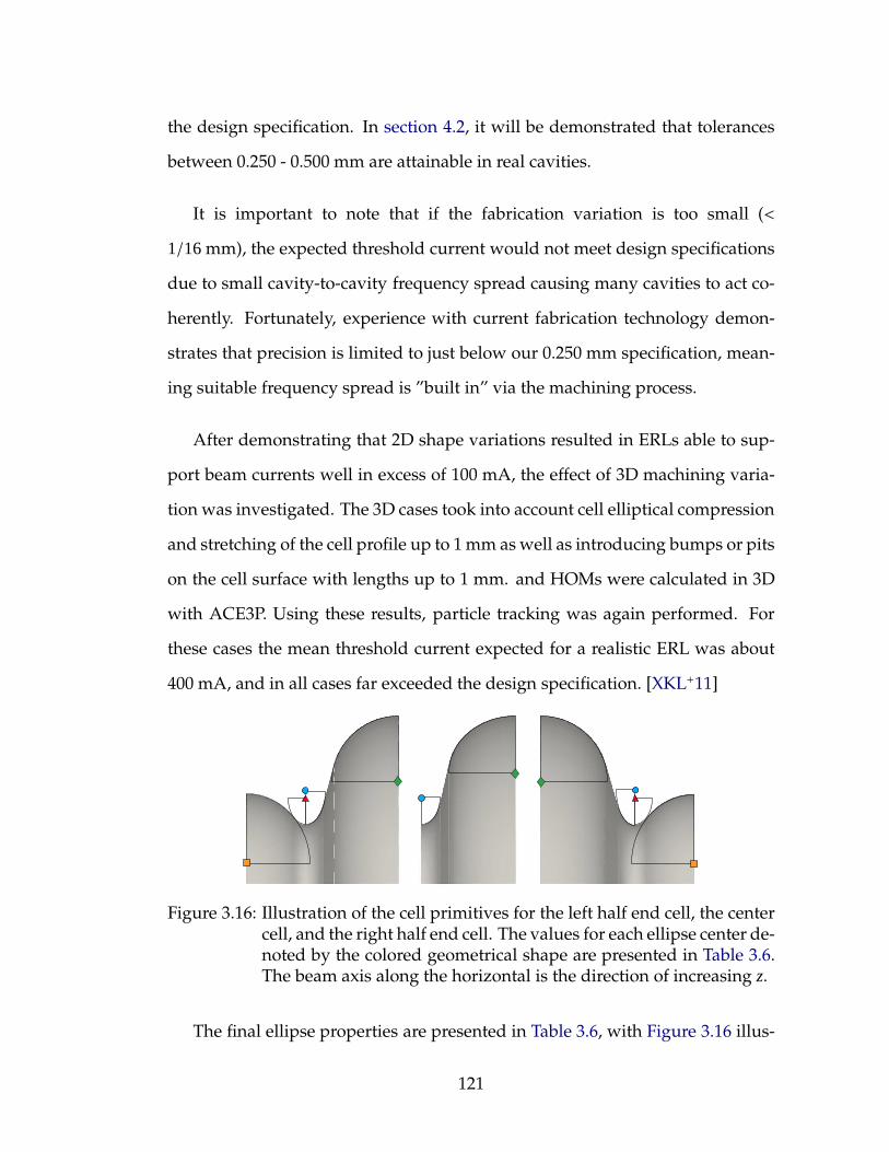
the design specification. In section 4.2, it will be demonstrated that tolerances
between 0.250 - 0.500 mm are attainable in real cavities.
It is important to note that if the fabrication variation is too small (<
1/16mm), the expected threshold current would not meet design specifications
due to small cavity-to-cavity frequency spread causing many cavities to act co-
herently. Fortunately, experience with current fabrication technology demon-
strates that precision is limited to just below our 0.250 mm specification, mean-
ing suitable frequency spread is ”built in” via the machining process.
After demonstrating that 2D shape variations resulted in ERLs able to sup-
port beam currents well in excess of 100 mA, the effect of 3D machining varia-
tion was investigated. The 3D cases took into account cell elliptical compression
and stretching of the cell profile up to 1 mm as well as introducing bumps or pits
on the cell surface with lengths up to 1 mm. and HOMs were calculated in 3D
with ACE3P. Using these results, particle tracking was again performed. For
these cases the mean threshold current expected for a realistic ERL was about
400 mA, and in all cases far exceeded the design specification. [XKL+11]
Figure 3.16: Illustration of the cell primitives for the left half end cell, the centercell, and the right half end cell. The values for each ellipse center de-noted by the colored geometrical shape are presented in Table 3.6.The beam axis along the horizontal is the direction of increasing z.
The final ellipse properties are presented in Table 3.6, with Figure 3.16 illus-
121
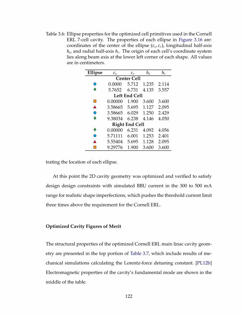
Table 3.6: Ellipse properties for the optimized cell primitives used in the CornellERL 7-cell cavity. The properties of each ellipse in Figure 3.16 are:coordinates of the center of the ellipse (cz, cr), longitudinal half-axishz, and radial half-axis hr. The origin of each cell’s coordinate systemlies along beam axis at the lower left corner of each shape. All valuesare in centimeters.
Ellipse cz cr hz hr
Center Cell0.0000 5.712 1.235 2.1145.7652 6.731 4.135 3.557
Left End Cell0.00000 1.900 3.600 3.6003.58665 5.695 1.127 2.0953.58665 6.029 1.250 2.4299.38034 6.238 4.146 4.050
Right End Cell0.00000 6.231 4.092 4.0565.71111 6.001 1.253 2.4015.55404 5.695 1.128 2.0959.29776 1.900 3.600 3.600
trating the location of each ellipse.
At this point the 2D cavity geometry was optimized and verified to satisfy
design design constraints with simulated BBU current in the 300 to 500 mA
range for realistic shape imperfections, which pushes the threshold current limit
three times above the requirement for the Cornell ERL.
Optimized Cavity Figures of Merit
The structural properties of the optimized Cornell ERL main linac cavity geom-
etry are presented in the top portion of Table 3.7, which include results of me-
chanical simulations calculating the Lorentz-force detuning constant. [PL12b]
Electromagnetic properties of the cavity’s fundamental mode are shown in the
middle of the table.
122

Table 3.7: Top: Structural properties and figures of merit for the optimizedmain-linac cavity for Cornell’s ERL. Middle: Fundamental mode fig-ures of merit. Bottom: Loss factors for the optimized main-linac cav-ity for Cornell’s ERL, with a σ = 0.6 mm electron bunch from a 2Dwakefield calculation with ABCI. [Chi94]
Structural PropertiesParameter Value UnitType of accelerating structure Standing wave —Accelerating Mode TM010, π-mode —Operating Gradient 16.2 MV/mIntrinsic quality factor, Q0 at 1.8 K > 2× 10¹⁰ —Loaded quality factor, QL 6.5× 10⁷ —Cavity half bandwidth 10 HzCell Iris diameter 36 mmBeam tube diameter 110 mmNumber of cells 7 —Active length 0.81 m∆ f /∆L 16.0 kHz/µmLorentz-force detuning constant 1 Hz/(MeV/m)2
Fundamental Mode Electromagnetic PropertiesParameter Value UnitFundamental Frequency 1300 MHzCell-to-cell coupling 2.2 %Geometry factor 270.7 Ω
R/Q (circuit definition) 387 Ω
Epeak/Eacc 2.06 —Hpeak/Eacc 4.196 mT/(MV/m)
Wakefield Loss FactorsParameter Value UnitTotal longitudinal loss factor 14.7 V/pcLongitudinal loss factor fromnon-fundamental modes
13.1 V/pc
Transverse loss factor 13.7 V/pc/m
The loss factor of a beam travelling through the structure was calculated
in 2D with a code ABCI. [Chi94] A 0.6 mm long Gaussian bunch was driven
through a string of 4 accelerating cavities–which was the maximum number of
cavities that could be simulated due to memory constraints–and the wakefield
was calculated up to 150 GHz. The loss factors are summarized in the bottom
123
section of Table 3.7.
The longitudinal loss factor, k||, relates the average HOM monopole power,
Pavg, generated by a beam current, Ib, consisting of bunch charges, qb, according
to
Pavg = k|| · qb · Ib. (3.20)
For the Cornell ERL, Pavg = 13.1 V/pC · 77 pC · 200 mA = 200 W, would be
expected for a large number of cavities with random HOM frequencies. This
power can be lower or higher depending on how far the beam harmonics
are from HOM frequencies. The design of the cavity ensures that no strong
monopole modes are near beam harmonics of 2600 MHz, preventing overload-
ing the HOM absorbers with monopole power.
3.3.1 High Power Coupler Design
The cavities in the ERL main linac will be operated at very high loaded quality
factors, due to the large external coupling, Qext , of the high power input coupler.
Because the energy transferred from the decelerated beam to the RF-cavity field
is equal to the energy transferred from the RF field to the accelerated beam in
an ideal ERL, there is virtually zero beam loading, and the optimal Qext only
depends on the typical detuning, ∆ f , [BBB+11]
Qext =f0
2∆ f. (3.21)
Estimates of the expected detuning suggest that 10 Hz is typical peak detuning
of the cavities in operation, meaning Qext = 6.5× 10⁷.
124
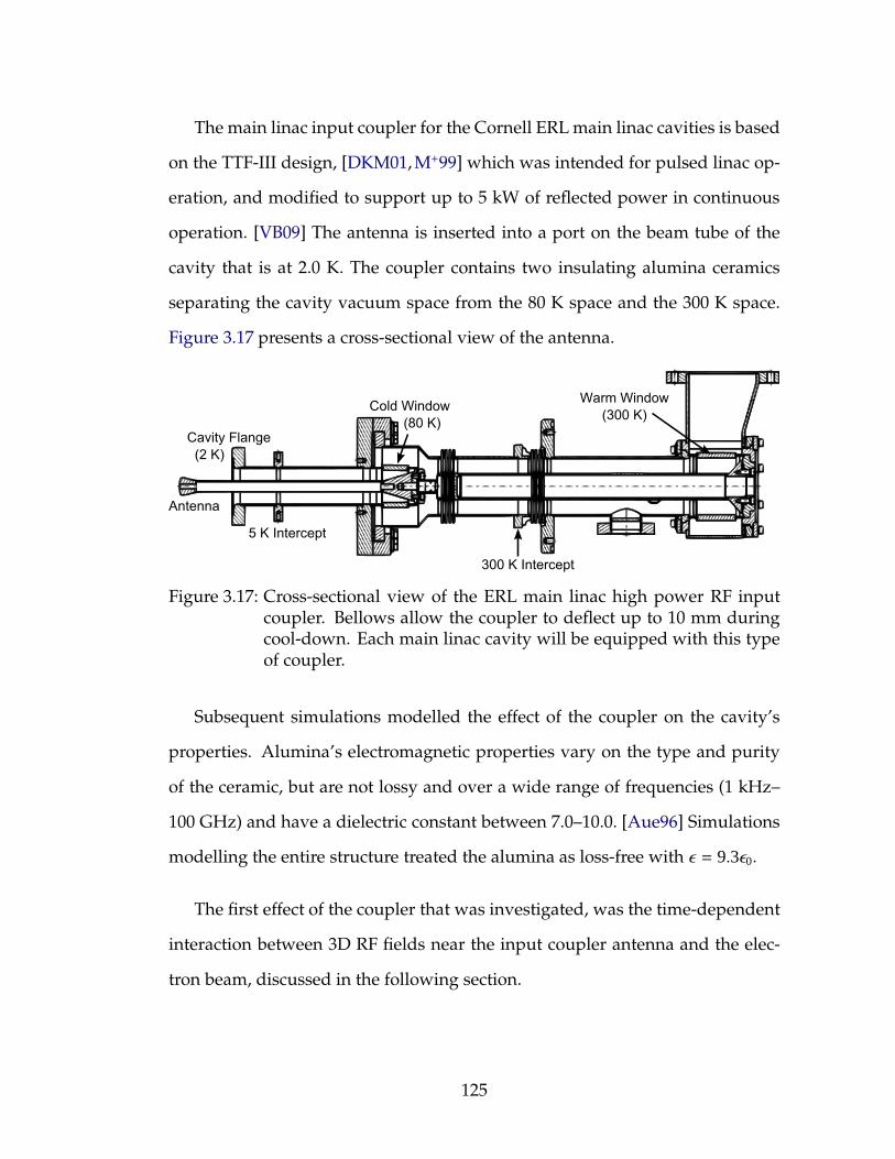
The main linac input coupler for the Cornell ERL main linac cavities is based
on the TTF-III design, [DKM01, M+99] which was intended for pulsed linac op-
eration, and modified to support up to 5 kW of reflected power in continuous
operation. [VB09] The antenna is inserted into a port on the beam tube of the
cavity that is at 2.0 K. The coupler contains two insulating alumina ceramics
separating the cavity vacuum space from the 80 K space and the 300 K space.
Figure 3.17 presents a cross-sectional view of the antenna.
Figure 3.17: Cross-sectional view of the ERL main linac high power RF inputcoupler. Bellows allow the coupler to deflect up to 10 mm duringcool-down. Each main linac cavity will be equipped with this typeof coupler.
Subsequent simulations modelled the effect of the coupler on the cavity’s
properties. Alumina’s electromagnetic properties vary on the type and purity
of the ceramic, but are not lossy and over a wide range of frequencies (1 kHz–
100 GHz) and have a dielectric constant between 7.0–10.0. [Aue96] Simulations
modelling the entire structure treated the alumina as loss-free with ǫ = 9.3ǫ0.
The first effect of the coupler that was investigated, was the time-dependent
interaction between 3D RF fields near the input coupler antenna and the elec-
tron beam, discussed in the following section.
125
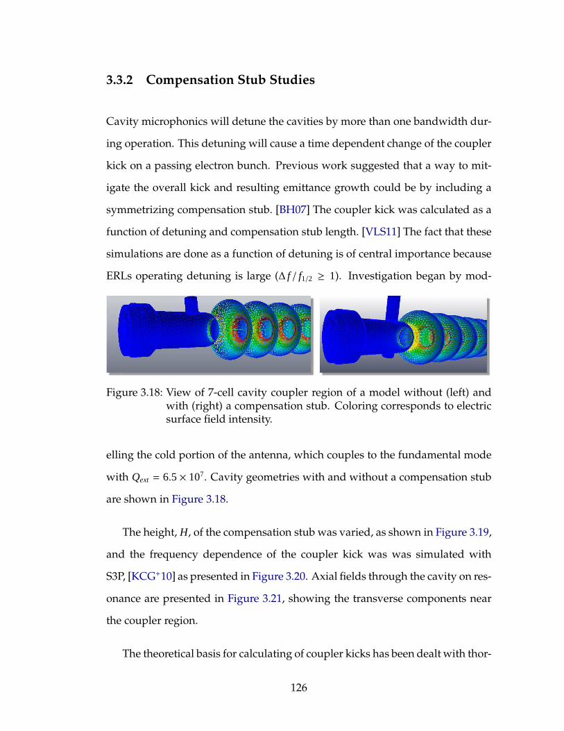
3.3.2 Compensation Stub Studies
Cavity microphonics will detune the cavities by more than one bandwidth dur-
ing operation. This detuning will cause a time dependent change of the coupler
kick on a passing electron bunch. Previous work suggested that a way to mit-
igate the overall kick and resulting emittance growth could be by including a
symmetrizing compensation stub. [BH07] The coupler kick was calculated as a
function of detuning and compensation stub length. [VLS11] The fact that these
simulations are done as a function of detuning is of central importance because
ERLs operating detuning is large (∆ f / f1/2 ≥ 1). Investigation began by mod-
Figure 3.18: View of 7-cell cavity coupler region of a model without (left) andwith (right) a compensation stub. Coloring corresponds to electricsurface field intensity.
elling the cold portion of the antenna, which couples to the fundamental mode
with Qext = 6.5× 10⁷. Cavity geometries with and without a compensation stub
are shown in Figure 3.18.
The height, H, of the compensation stub was varied, as shown in Figure 3.19,
and the frequency dependence of the coupler kick was was simulated with
S3P, [KCG+10] as presented in Figure 3.20. Axial fields through the cavity on res-
onance are presented in Figure 3.21, showing the transverse components near
the coupler region.
The theoretical basis for calculating of coupler kicks has been dealt with thor-
126
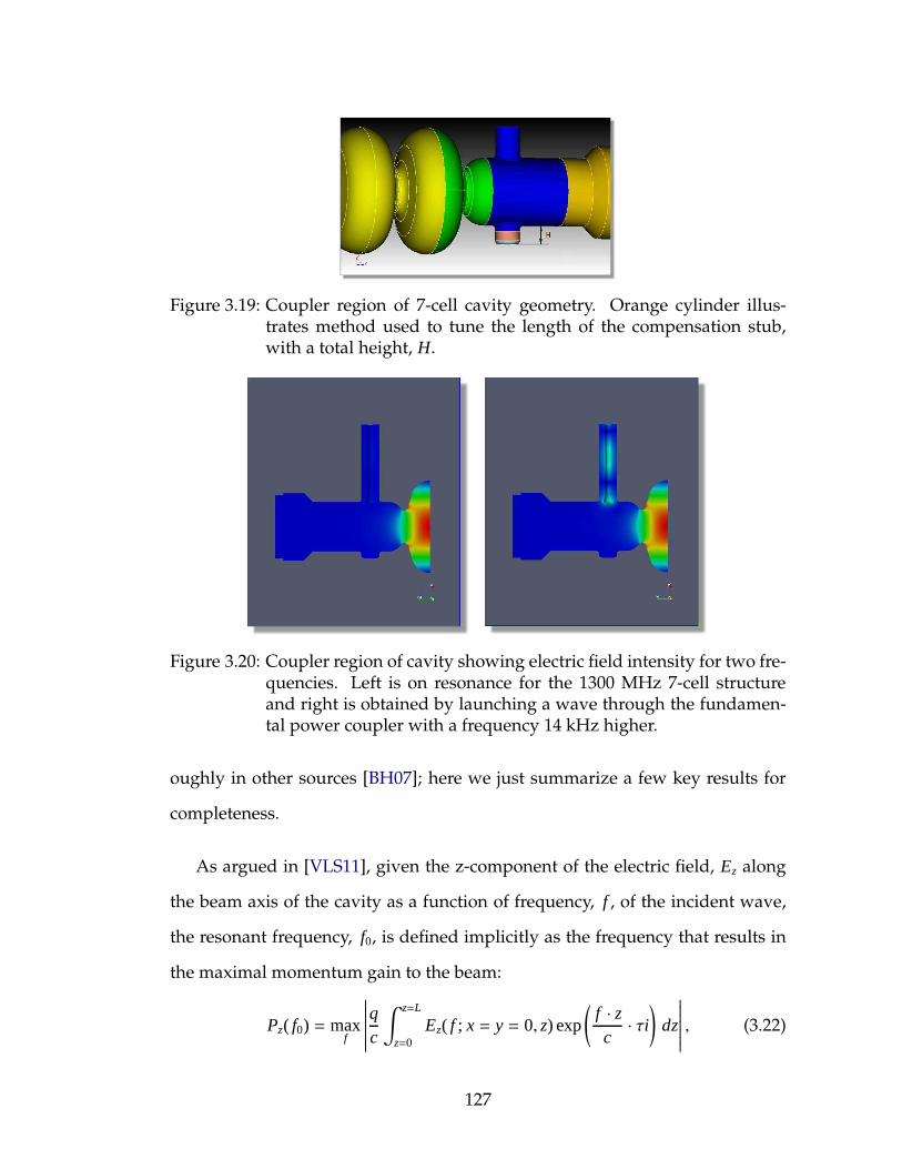
Figure 3.19: Coupler region of 7-cell cavity geometry. Orange cylinder illus-trates method used to tune the length of the compensation stub,with a total height, H.
Figure 3.20: Coupler region of cavity showing electric field intensity for two fre-quencies. Left is on resonance for the 1300 MHz 7-cell structureand right is obtained by launching a wave through the fundamen-tal power coupler with a frequency 14 kHz higher.
oughly in other sources [BH07]; here we just summarize a few key results for
completeness.
As argued in [VLS11], given the z-component of the electric field, Ez along
the beam axis of the cavity as a function of frequency, f , of the incident wave,
the resonant frequency, f0, is defined implicitly as the frequency that results in
the maximal momentum gain to the beam:
Pz( f0) = maxf
∣∣∣∣∣∣∣
qc
∫ z=L
z=0Ez( f ; x = y = 0, z) exp
(
f · zc· τi
)
dz
∣∣∣∣∣∣∣
, (3.22)
127
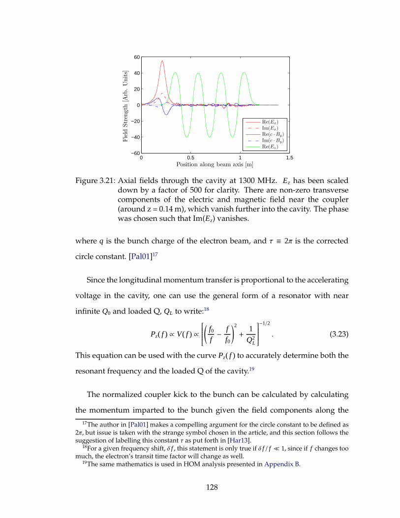
0 0.5 1 1.5−60
−40
−20
0
20
40
60
Position along beam axis [m]
Fie
ldStr
ength
[Arb
.U
nits]
Re(Ex)Im(Ex)Re(c ·By)Im(c ·By)Re(Ez)
Figure 3.21: Axial fields through the cavity at 1300 MHz. Ez has been scaleddown by a factor of 500 for clarity. There are non-zero transversecomponents of the electric and magnetic field near the coupler(around z = 0.14 m), which vanish further into the cavity. The phasewas chosen such that Im(Ez) vanishes.
where q is the bunch charge of the electron beam, and τ ≡ 2π is the corrected
circle constant. [Pal01]17
Since the longitudinal momentum transfer is proportional to the accelerating
voltage in the cavity, one can use the general form of a resonator with near
infinite Q0 and loaded Q, QL to write:18
Pz( f ) ∝ V( f ) ∝
(
f0f− f
f0
)2
+1
Q2L
−1/2
. (3.23)
This equation can be used with the curve Pz( f ) to accurately determine both the
resonant frequency and the loaded Q of the cavity.19
The normalized coupler kick to the bunch can be calculated by calculating
the momentum imparted to the bunch given the field components along the
17The author in [Pal01] makes a compelling argument for the circle constant to be defined as2π, but issue is taken with the strange symbol chosen in the article, and this section follows thesuggestion of labelling this constant τ as put forth in [Har13].
18For a given frequency shift, δ f , this statement is only true if δ f / f ≪ 1, since if f changes toomuch, the electron’s transit time factor will change as well.
19The same mathematics is used in HOM analysis presented in Appendix B.
128
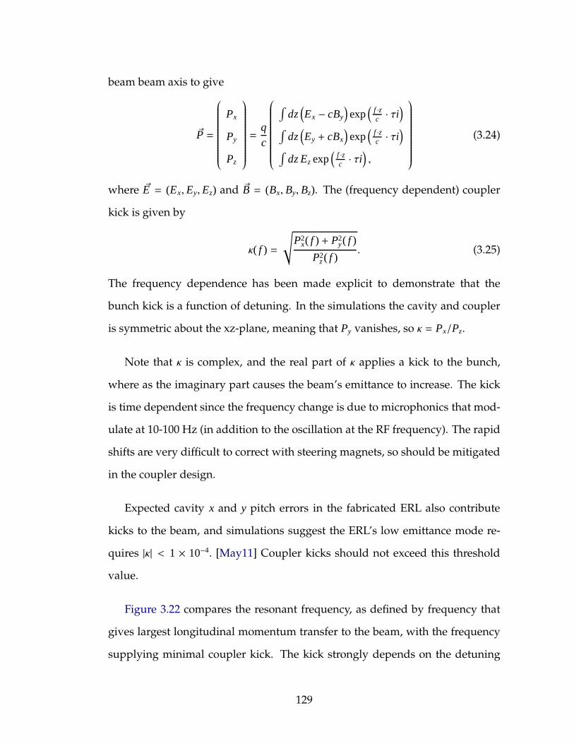
beam beam axis to give
~P =
Px
Py
Pz
=qc
∫
dz(
Ex − cBy
)
exp(
f ·zc · τi
)
∫
dz(
Ey + cBx
)
exp(
f ·zc · τi
)
∫
dz Ez exp(
f ·zc · τi
)
,
(3.24)
where ~E = (Ex, Ey, Ez) and ~B = (Bx, By, Bz). The (frequency dependent) coupler
kick is given by
κ( f ) =
√
P2x( f ) + P2
y( f )
P2z ( f )
. (3.25)
The frequency dependence has been made explicit to demonstrate that the
bunch kick is a function of detuning. In the simulations the cavity and coupler
is symmetric about the xz-plane, meaning that Py vanishes, so κ = Px/Pz.
Note that κ is complex, and the real part of κ applies a kick to the bunch,
where as the imaginary part causes the beam’s emittance to increase. The kick
is time dependent since the frequency change is due to microphonics that mod-
ulate at 10-100 Hz (in addition to the oscillation at the RF frequency). The rapid
shifts are very difficult to correct with steering magnets, so should be mitigated
in the coupler design.
Expected cavity x and y pitch errors in the fabricated ERL also contribute
kicks to the beam, and simulations suggest the ERL’s low emittance mode re-
quires |κ| < 1 × 10⁻⁴. [May11] Coupler kicks should not exceed this threshold
value.
Figure 3.22 compares the resonant frequency, as defined by frequency that
gives largest longitudinal momentum transfer to the beam, with the frequency
supplying minimal coupler kick. The kick strongly depends on the detuning
129
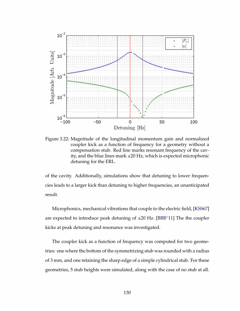
−100 −50 0 50 10010
−6
10−5
10−4
10−3
10−2
Detuning [Hz]
Magnitude
[Arb
.U
nits]
|Pz||κ|
Figure 3.22: Magnitude of the longitudinal momentum gain and normalizedcoupler kick as a function of frequency for a geometry without acompensation stub. Red line marks resonant frequency of the cav-ity, and the blue lines mark ±20 Hz, which is expected microphonicdetuning for the ERL.
of the cavity. Additionally, simulations show that detuning to lower frequen-
cies leads to a larger kick than detuning to higher frequencies, an unanticipated
result.
Microphonics, mechanical vibrations that couple to the electric field, [KSS67]
are expected to introduce peak detuning of ±20 Hz. [BBB+11] The the coupler
kicks at peak detuning and resonance was investigated.
The coupler kick as a function of frequency was computed for two geome-
tries: one where the bottom of the symmetrizing stub was rounded with a radius
of 3 mm, and one retaining the sharp edge of a simple cylindrical stub. For these
geometries, 5 stub heights were simulated, along with the case of no stub at all.
130
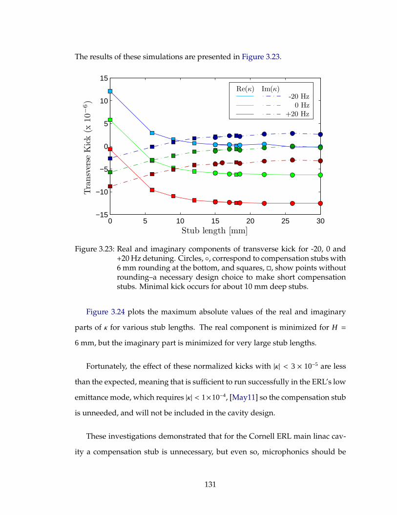
The results of these simulations are presented in Figure 3.23.
0 5 10 15 20 25 30−15
−10
−5
0
5
10
15Tra
nsv
erse
Kick
(x10−
6)
Stub length [mm]
Re(κ) Im(κ)-20 Hz
0 Hz+20 Hz
Figure 3.23: Real and imaginary components of transverse kick for -20, 0 and+20 Hz detuning. Circles, , correspond to compensation stubs with6 mm rounding at the bottom, and squares, , show points withoutrounding–a necessary design choice to make short compensationstubs. Minimal kick occurs for about 10 mm deep stubs.
Figure 3.24 plots the maximum absolute values of the real and imaginary
parts of κ for various stub lengths. The real component is minimized for H =
6 mm, but the imaginary part is minimized for very large stub lengths.
Fortunately, the effect of these normalized kicks with |κ| < 3 × 10⁻⁵ are less
than the expected, meaning that is sufficient to run successfully in the ERL’s low
emittance mode, which requires |κ| < 1×10⁻⁴, [May11] so the compensation stub
is unneeded, and will not be included in the cavity design.
These investigations demonstrated that for the Cornell ERL main linac cav-
ity a compensation stub is unnecessary, but even so, microphonics should be
131

0 5 10 15 20 25 302
4
6
8
10
12
14
Stub length [mm]
Tra
nsv
erse
Kick
(x10−
6)
Max |Re(κ)|Max |Im(κ)|
Figure 3.24: Maximum absolute values of the real and imaginary parts of thecoupler kick, κ as a function of stub length over a detuning range of±20 Hz.
kept small since they can cause the transverse kick to increase by more than an
order of magnitude over the ±20 Hz bandwidth. This effect may be worse in
accelerators with lower Qext , so for this type of machine, this effect should be
investigated.
3.3.3 3D HOM Simulations
To investigate the influence of the high power coupler on the higher-order mode
spectrum, simulations were performed with Omega3P. The center planes of the
HOM loads and the rectangular waveguide port were set to either electric or
magnetic boundary conditions. Several types of modes were located, finding
monopole, dipole, quadrupole, sextupole and octupole HOMs as well as some
132
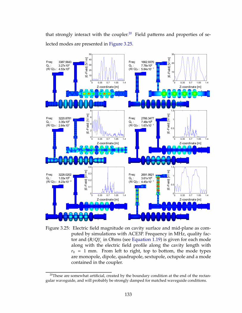
that strongly interact with the coupler.20 Field patterns and properties of se-
lected modes are presented in Figure 3.25.
Figure 3.25: Electric field magnitude on cavity surface and mid-plane as com-puted by simulations with ACE3P. Frequency in MHz, quality fac-tor and (R/Q)′⊥ in Ohms (see Equation 1.19) is given for each modealong with the electric field profile along the cavity length withr0 = 1 mm. From left to right, top to bottom, the mode typesare monopole, dipole, quadrupole, sextupole, octupole and a modecontained in the coupler.
20These are somewhat artificial, created by the boundary condition at the end of the rectan-gular waveguide, and will probably be strongly damped for matched waveguide conditions.
133
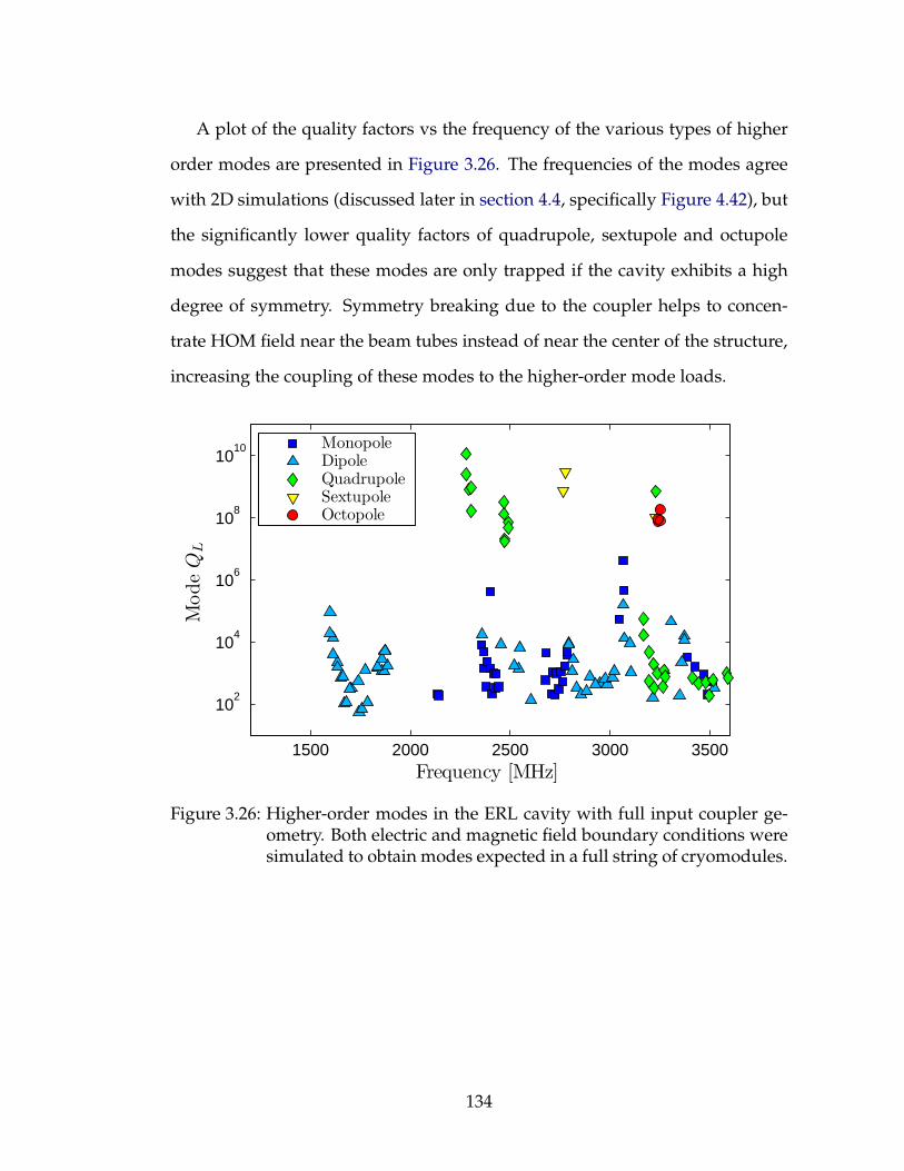
A plot of the quality factors vs the frequency of the various types of higher
order modes are presented in Figure 3.26. The frequencies of the modes agree
with 2D simulations (discussed later in section 4.4, specifically Figure 4.42), but
the significantly lower quality factors of quadrupole, sextupole and octupole
modes suggest that these modes are only trapped if the cavity exhibits a high
degree of symmetry. Symmetry breaking due to the coupler helps to concen-
trate HOM field near the beam tubes instead of near the center of the structure,
increasing the coupling of these modes to the higher-order mode loads.
1500 2000 2500 3000 3500
102
104
106
108
1010
Frequency [MHz]
Mode
QL
MonopoleDipoleQuadrupoleSextupoleOctopole
Figure 3.26: Higher-order modes in the ERL cavity with full input coupler ge-ometry. Both electric and magnetic field boundary conditions weresimulated to obtain modes expected in a full string of cryomodules.
134

3.4 Cavity Classes
Since BBU current can be lowered by multiple cavities acting coherently, by
shifting the relative frequency of HOMs from cavity to cavity, the effective reso-
nant kick given to the beam through the machine can be reduced. An increase in
the threshold current has been seen when taking machining perturbations into
account (recall Figure 3.15). Small dimensional errors change the shape of each
cavity slightly and introduce a relative HOM frequency spread from cavity to
cavity, and thus increase the threshold current.
It was shown in Figure 3.15 that simply relaxing machining tolerances to
ever larger values to increase the frequency spread is not a way to increase
the beam breakup current because too large shape perturbations (> 0.500 mm
for the optimized cavity) can lead to trapped modes certain cavity shapes lead
to trapped modes that will strongly reduce BBU current. [VL11] Instead, ad-
ditional frequency spread can be introduced in a controlled way by designing
multiple cavity center cell classes can be designed that have roughly the same
fundamental mode properties, while having higher-order modes at different
frequencies.
The additional cavities are made by selecting a new center cell design and
optimizing the end cells for this center cell shape. By using several cavity shapes
in the same ERL, having different HOM spectra, the relative cavity-to-cavity
frequency spread of the cavities is increased.
The four parameters characterizing a center cell cavity were varied by
±5 mm in 1 mm steps, and the frequencies of 0- and π-modes, f0 and fπ re-
spectively, were calculated to obtain the first 6 dipole HOM dispersion curves
135

0 20 40 60 80 100 120 140 160 1801500
2000
2500
3000
3500
Phase [Deg]
Fre
quen
cy[M
Hz]
Figure 3.27: Dispersion curves for multiple center cell shapes, demonstratingthat a large cavity-to-cavity frequency spread can be obtained whilekeeping similar fundamental mode properties.
for each geometry. Dispersion curves are calculated from these modes via
f (φ) = f0√
1+ 2kcc(1− cosφ), (3.26)
kcc ≡f 2π − f 2
0
2 f 20
, (3.27)
where kcc is the cell-to-cell coupling factor of the passband. [Lie01] Note that for
electric coupling, the π-mode has a higher frequency than the 0-mode, where as
for magnetic coupling, the reverse is true. [Sch11]
Dispersion curves are presented in Figure 3.27 for center cells that are within
5% of the optimized cavity’s R/Q · G and Hpk/Eacc; Epk/Eacc was maintained at
2.1. In addition, only cavity geometries with | f0− fπ| > 20MHz were considered,
since cavities with narrow passbands are not robust with respect to machining
variation.
136
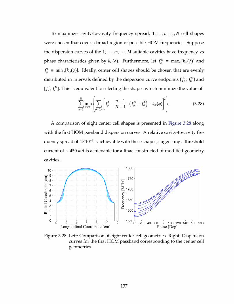
To maximize cavity-to-cavity frequency spread, 1, . . . , n, . . . ,N cell shapes
were chosen that cover a broad region of possible HOM frequencies. Suppose
the dispersion curves of the 1, . . . ,m, . . . , M suitable cavities have frequency vs
phase characteristics given by km(φ). Furthermore, let f Uφ ≡ maxm[km(φ)] and
f Lφ ≡ minm[km(φ)]. Ideally, center cell shapes should be chosen that are evenly
distributed in intervals defined by the dispersion curve endpoints [ f L0 , f U
0 ] and
[ f Lπ , f U
π ]. This is equivalent to selecting the shapes which minimize the value of
N∑
n=1
minm∈M
∑
φ=0,π
[
f Lφ +
n − 1N − 1
·(
f Uφ − f L
φ
)
− km(φ)
]2
. (3.28)
A comparison of eight center cell shapes is presented in Figure 3.28 along
with the first HOM passband dispersion curves. A relative cavity-to-cavity fre-
quency spread of 4×10⁻³ is achievable with these shapes, suggesting a threshold
current of ∼ 450mA is achievable for a linac constructed of modified geometry
cavities.
Figure 3.28: Left: Comparison of eight center-cell geometries. Right: Dispersioncurves for the first HOM passband corresponding to the center cellgeometries.
137
3.5 Conclusion of Cavity Design
This section has presented a systematic process used to design the main cavity
for the 15 MeV to 5 GeV linear accelerating section of Cornell’s ERL. Parallel
computing was employed to the constrained optimization problem of mitigat-
ing the effect of higher-order modes in the cavity via the introduction of a beam
breakup parameter, eschewing the need for costly particle tracking simulations
at each iteration step.
The optimized cavity has been shown to be stable under small machining
variations, verified by both 2D and 3D simulations. Particle tracking demon-
strated that as long as dimensional variation introduced by the machining pro-
cess are less than ±0.5 mm, machine current will exceed the design specification.
Specifically, simulations of realistic ERLs comprised of cavities with unique
HOM spectra show that threshold current in excess of 300 mA can be expected
for the full machine, three times better than the 100 mA requirement.
Simulations incorporating 3D features such as the main linac coupler
demonstrated also that quadrupole higher-order modes are sufficiently damped
by beamline absorbers. The overall effect of the coupler is to break symmetry,
which further assists in reducing the the Q of the otherwise trapped first two
quadrupole passbands in the cavity via mixing to propagating modes in the
beam tubes.
Overall the structure has been throughly verified to exceed the requirements
for the Cornell ERL. In the next chapter, the fabrication and experimental quali-
fication of the prototype of this structure is presented.
138
CHAPTER 4
PROTOTYPE CAVITY FABRICATION AND COMMISSIONING
This chapter discusses the process of taking the optimized cavity geometry
design obtained in the previous chapter and turning it into a structure quali-
fied to be used in an operational particle accelerator. Qualification consists of
five steps: 1) Demonstrate that tight fabrication tolerances can be achieved. 2)
Show that the fundamental mode has a very high intrinsic quality factor, Q0. 3)
Validate that higher-order modes are strongly damped. 4) Establish the proper
operation of auxiliary components such as the RF input coupler, HOM beam-
line loads, and frequency tuner. 5) Study the mechanical properties of the cavity,
showing that they are suitable for ERL operation.
This chapter begins by outlining the fabrication choices made for the Cor-
nell ERL main linac cavity, the production of the first prototype cavity and the
assembly, and installation methods used to measure the RF properties of the
structure. Next, qualifications of the fundamental mode in vertical and hori-
zontal tests are presented,1 in which the cavity set a world record Q0 = 1× 10¹¹
for a multicell cavity in a realistic accelerator environment, far exceeding the
Cornell ERL Q0 design specification of 2 × 10¹⁰. Finally, the properties of the
prototype cavity’s higher-order mode (HOM) spectrum are measured and it is
found that all measured dipole HOMs are strongly damped, suggesting that an
ERL constructed from this type of 7-cell cavity should be able to support con-
1Vertical measurements are simple tests that can establish Q0 of a resonator, but are unrealis-tic of the conditions within a particle accelerator. Horizontal testing probes the performance ofa cavity in a similar configuration as in an operational accelerator.
139
tinuous beam current in excess of the 100 mA Cornell ERL design specification.
4.1 SRF Accelerating Cavity Fabrication Considerations
Modern particle accelerators relying on superconducting technology for their
accelerating structures use niobium as the material for the RF surface layer.
Many techniques exist to fabricate accelerating cavities with niobium RF sur-
face layers, include forming structures from bulk Nb, explosion bonding a layer
of Nb onto a Cu substrate, or various experimental techniques to deposit thin
films of Nb onto metallic substrates, a process known as sputtering. [PKH98]
All three methods have successfully been used to produce accelerating cavities,
with explosion bonding Nb onto Cu used for the prototype cavities in HERA
at DESY, [DEM+87]2 sputtering Nb on Cu for the superconducting cavities at
LEP and the LHC at CERN, [Sla97,BCH+99] and bulk Nb cavities used at many
sites around the world including at CEBAF at Jefferson Laboratory. [DIPK91]
The design for Cornell’s Energy Recovery Linac proposes to form the main
linac accelerating structures out of sheet metal Nb, [BBB+11] a method that
has been successfully demonstrated at many laboratories around the world,
and is the proposed standard for the prospective International Linear Collider
project. [SAE+13]
Bulk niobium material is available in high purity, typically with residual
resistivity ratios (RRR) in excess of 300, and can be produced with either large or
fine grain sizes (grain diameters >10 cm or ∼50 µm respectively). [PKH98] While
large grain material has been used to successfully fabricate SRF cavities with
high quality factors at medium accelerating gradients (12-18 MV/m), [KMC+05,
2The cavities actually used in the HERA upgrade were made of bulk niobium. [DMM+95]
140
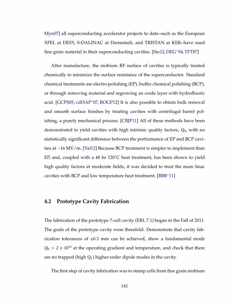
Myn07] all superconducting accelerator projects to date–such as the European
XFEL at DESY, S-DALINAC at Darmstadt, and TRISTAN at KEK–have used
fine grain material in their superconducting cavities. [Sin12, DEG+94, TFT87]
After manufacture, the niobium RF surface of cavities is typically treated
chemically to minimize the surface resistance of the superconductor. Standard
chemical treatments are electro-polishing (EP), buffer chemical polishing (BCP),
or through removing material and regrowing an oxide layer with hydrofluoric
acid. [GCPS05, vdHAP+07, ROGP12] It is also possible to obtain bulk removal
and smooth surface finishes by treating cavities with centrifugal barrel pol-
ishing, a purely mechanical process. [CBJP11] All of these methods have been
demonstrated to yield cavities with high intrinsic quality factors, Q0, with no
statistically significant difference between the performance of EP and BCP cavi-
ties at ∼16 MV/m. [Val12] Because BCP treatment is simpler to implement than
EP, and, coupled with a 48 hr 120C heat treatment, has been shown to yield
high quality factors at moderate fields, it was decided to treat the main linac
cavities with BCP and low temperature heat treatment. [BBB+11]
4.2 Prototype Cavity Fabrication
The fabrication of the prototype 7-cell cavity (ERL 7.1) began in the Fall of 2011.
The goals of the prototype cavity were threefold: Demonstrate that cavity fab-
rication tolerances of ±0.5 mm can be achieved, show a fundamental mode
Q0 > 2 × 10¹⁰ at the operating gradient and temperature, and check that there
are no trapped (high QL) higher-order dipole modes in the cavity.
The first step of cavity fabrication was to stamp cells from fine grain niobium
141
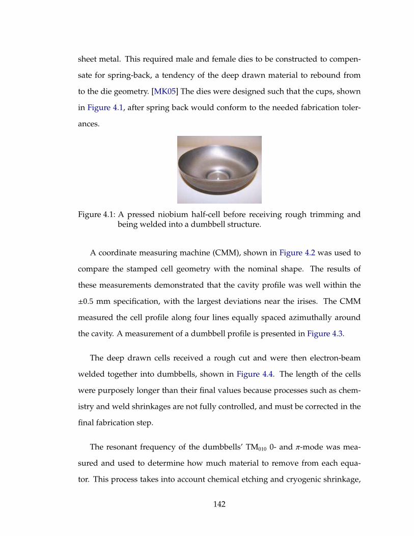
sheet metal. This required male and female dies to be constructed to compen-
sate for spring-back, a tendency of the deep drawn material to rebound from
to the die geometry. [MK05] The dies were designed such that the cups, shown
in Figure 4.1, after spring back would conform to the needed fabrication toler-
ances.
Figure 4.1: A pressed niobium half-cell before receiving rough trimming andbeing welded into a dumbbell structure.
A coordinate measuring machine (CMM), shown in Figure 4.2 was used to
compare the stamped cell geometry with the nominal shape. The results of
these measurements demonstrated that the cavity profile was well within the
±0.5 mm specification, with the largest deviations near the irises. The CMM
measured the cell profile along four lines equally spaced azimuthally around
the cavity. A measurement of a dumbbell profile is presented in Figure 4.3.
The deep drawn cells received a rough cut and were then electron-beam
welded together into dumbbells, shown in Figure 4.4. The length of the cells
were purposely longer than their final values because processes such as chem-
istry and weld shrinkages are not fully controlled, and must be corrected in the
final fabrication step.
The resonant frequency of the dumbbells’ TM010 0- and π-mode was mea-
sured and used to determine how much material to remove from each equa-
tor. This process takes into account chemical etching and cryogenic shrinkage,
142
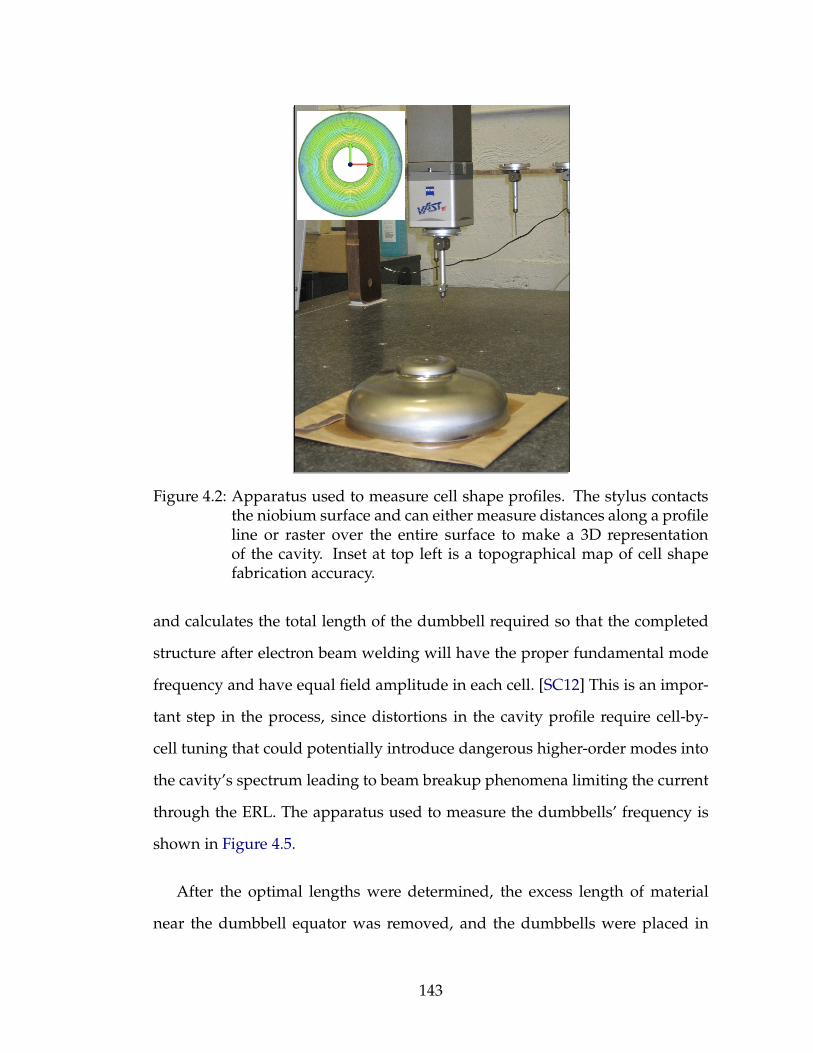
Figure 4.2: Apparatus used to measure cell shape profiles. The stylus contactsthe niobium surface and can either measure distances along a profileline or raster over the entire surface to make a 3D representationof the cavity. Inset at top left is a topographical map of cell shapefabrication accuracy.
and calculates the total length of the dumbbell required so that the completed
structure after electron beam welding will have the proper fundamental mode
frequency and have equal field amplitude in each cell. [SC12] This is an impor-
tant step in the process, since distortions in the cavity profile require cell-by-
cell tuning that could potentially introduce dangerous higher-order modes into
the cavity’s spectrum leading to beam breakup phenomena limiting the current
through the ERL. The apparatus used to measure the dumbbells’ frequency is
shown in Figure 4.5.
After the optimal lengths were determined, the excess length of material
near the dumbbell equator was removed, and the dumbbells were placed in
143

Figure 4.3: Measurements from CMM of a dumbbell cavity. The coordinate axesare in inches. Black dotted line denotes the nominal dumbbell shape.The red lines denote normal deviation from the nominal cavity shapeof 0.125mm, with 50x magnification. The red circles show the pointsof furthest deviation, either above the nominal value or below. Thefarthest discrepancy from the nominal value in this case is near theiris with a deviation of 0.38 mm.
nitric acid (30 min/side) to remove residual copper from the cells. The cells were
then ultrasonically cleaned with a hot water (38 - 60C) Liqui-Nox R© solution for
15 minutes. Subsequently, the cups were rinsed to remove any soap residue
and ultrasonically cleaned in hot de-ionized water for an additional 15 minutes,
followed by a bulk BCP.
Each BCP used acid at an initial temperature between -20 and -17 C. The
BCP was complete when either 16 minutes had passed or the acid tempera-
ture increased to -9C. After BCP, the oxide layer was allowed to regrow in de-
ionized water for four hours, and was then dried with a stream of high pressure
pure nitrogen gas for 1 hour and delivered for electron beam welding. [Car11]
After the dumbbells were welded to form the completed 7-cell structure, the
144
Figure 4.4: Cells after being welded to form dumbbells. These cells were sub-sequently measured to determine final trimming, and welded into afull cavity.
room temperature resonant frequency of the cavity’s TM010,π mode was mea-
sured to be 1298.623 MHz, close to the pre-chemistry goal of 1298.985 MHz.
[She11] A bead pull [Sch92] was performed to measure the field flatness3 of the
TM010,π mode and found the cavity was 95.7% field flat. These results demon-
strate precise control over the fabrication process.
Following initial measurements, the cavity received a 150 µm BCP, followed
by a 650C bake for 12 hours. Subsequent tuning of the cavity4 reached 95.1%
field flatness with a resonant frequency of 1297.521 MHz. The room tempera-
ture, post-etch target frequency of 1297.425 MHz [She11] was obtained by a final
10 µm BCP. The field profile of the cavity is presented in Figure 4.6.
Next, the cavity was cleaned by high-pressure rinsing (HPR) with de-ionized
water. During the HPR, the side port used for the high-power RF coupler was
blanked off as well as one cavity flange to help maintain cleanliness of the SRF
3Field flatness is defined as the ratio of the average of the peak amplitudes in each cell overthe maximum cell amplitude.
4Tuning is achieved by stretching and compressing the cells of a cavity.
145

Figure 4.5: A dumbbell inside the frequency measurement apparatus, used todetermine how much material to trim from the equator region sothat after welding the cavity has the proper resonant frequency. Thescrew allows the same force to be applied to each dumbbell, pre-venting unequal loading which could effect the measured resonantfrequency. Image reproduced from [SC12].
surface while drying and assembly. After the initial 8 hour HPR, a field probe
with Qext = 3 × 10¹¹ was installed on the cavity, the top beam tube was sealed
and the cavity was HPRed for an additional 8 hours.
The final assembly step after the second HPR was to connect a viking horn
connector having the axial coupler (Qext = 2 × 10¹⁰) and vacuum connection
to the cavity, thereby allowing evacuation of the cavity space. The cavity was
braced and slowly evacuated until the vacuum was better than 10−6 Torr. The
cavity was removed from the clean room, assembled onto a vertical test stand
and received a low temperature heat treatment by baking the cavity at 120C for
146
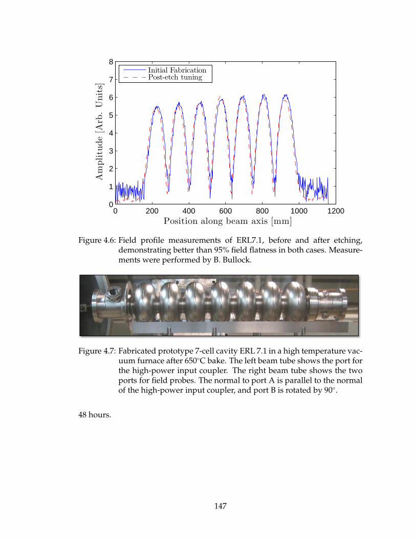
0 200 400 600 800 1000 12000
1
2
3
4
5
6
7
8
Position along beam axis [mm]
Am
plitu
de
[Arb
.U
nit
s]
Initial FabricationPost-etch tuning
Figure 4.6: Field profile measurements of ERL7.1, before and after etching,demonstrating better than 95% field flatness in both cases. Measure-ments were performed by B. Bullock.
Figure 4.7: Fabricated prototype 7-cell cavity ERL 7.1 in a high temperature vac-uum furnace after 650C bake. The left beam tube shows the port forthe high-power input coupler. The right beam tube shows the twoports for field probes. The normal to port A is parallel to the normalof the high-power input coupler, and port B is rotated by 90.
48 hours.
147
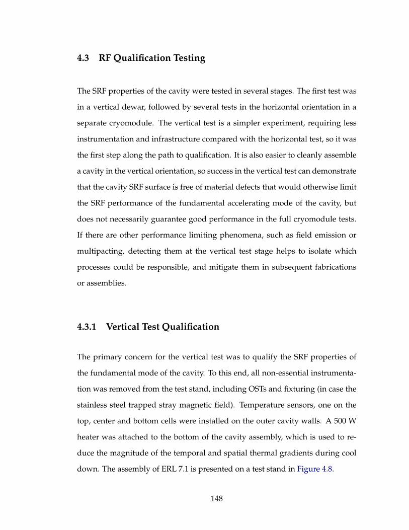
4.3 RF Qualification Testing
The SRF properties of the cavity were tested in several stages. The first test was
in a vertical dewar, followed by several tests in the horizontal orientation in a
separate cryomodule. The vertical test is a simpler experiment, requiring less
instrumentation and infrastructure compared with the horizontal test, so it was
the first step along the path to qualification. It is also easier to cleanly assemble
a cavity in the vertical orientation, so success in the vertical test can demonstrate
that the cavity SRF surface is free of material defects that would otherwise limit
the SRF performance of the fundamental accelerating mode of the cavity, but
does not necessarily guarantee good performance in the full cryomodule tests.
If there are other performance limiting phenomena, such as field emission or
multipacting, detecting them at the vertical test stage helps to isolate which
processes could be responsible, and mitigate them in subsequent fabrications
or assemblies.
4.3.1 Vertical Test Qualification
The primary concern for the vertical test was to qualify the SRF properties of
the fundamental mode of the cavity. To this end, all non-essential instrumenta-
tion was removed from the test stand, including OSTs and fixturing (in case the
stainless steel trapped stray magnetic field). Temperature sensors, one on the
top, center and bottom cells were installed on the outer cavity walls. A 500 W
heater was attached to the bottom of the cavity assembly, which is used to re-
duce the magnitude of the temporal and spatial thermal gradients during cool
down. The assembly of ERL 7.1 is presented on a test stand in Figure 4.8.
148
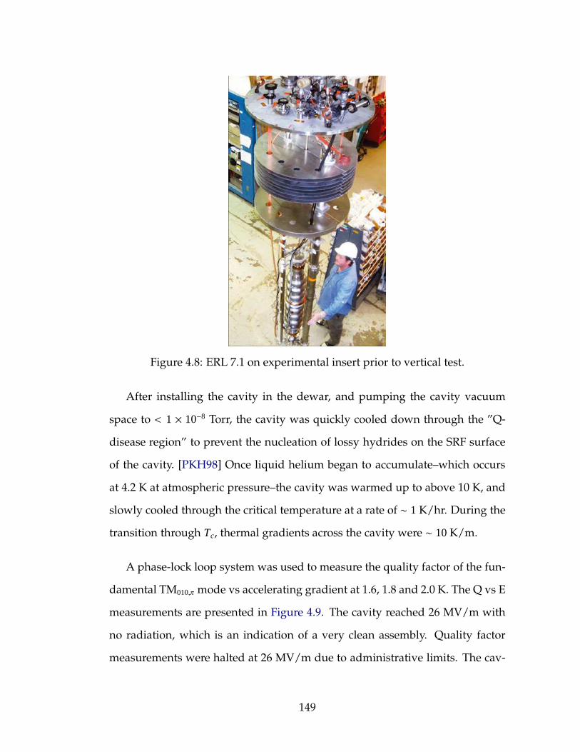
Figure 4.8: ERL 7.1 on experimental insert prior to vertical test.
After installing the cavity in the dewar, and pumping the cavity vacuum
space to < 1 × 10⁻⁸ Torr, the cavity was quickly cooled down through the ”Q-
disease region” to prevent the nucleation of lossy hydrides on the SRF surface
of the cavity. [PKH98] Once liquid helium began to accumulate–which occurs
at 4.2 K at atmospheric pressure–the cavity was warmed up to above 10 K, and
slowly cooled through the critical temperature at a rate of ∼ 1 K/hr. During the
transition through Tc, thermal gradients across the cavity were ∼ 10K/m.
A phase-lock loop system was used to measure the quality factor of the fun-
damental TM010,π mode vs accelerating gradient at 1.6, 1.8 and 2.0 K. The Q vs E
measurements are presented in Figure 4.9. The cavity reached 26 MV/m with
no radiation, which is an indication of a very clean assembly. Quality factor
measurements were halted at 26 MV/m due to administrative limits. The cav-
149
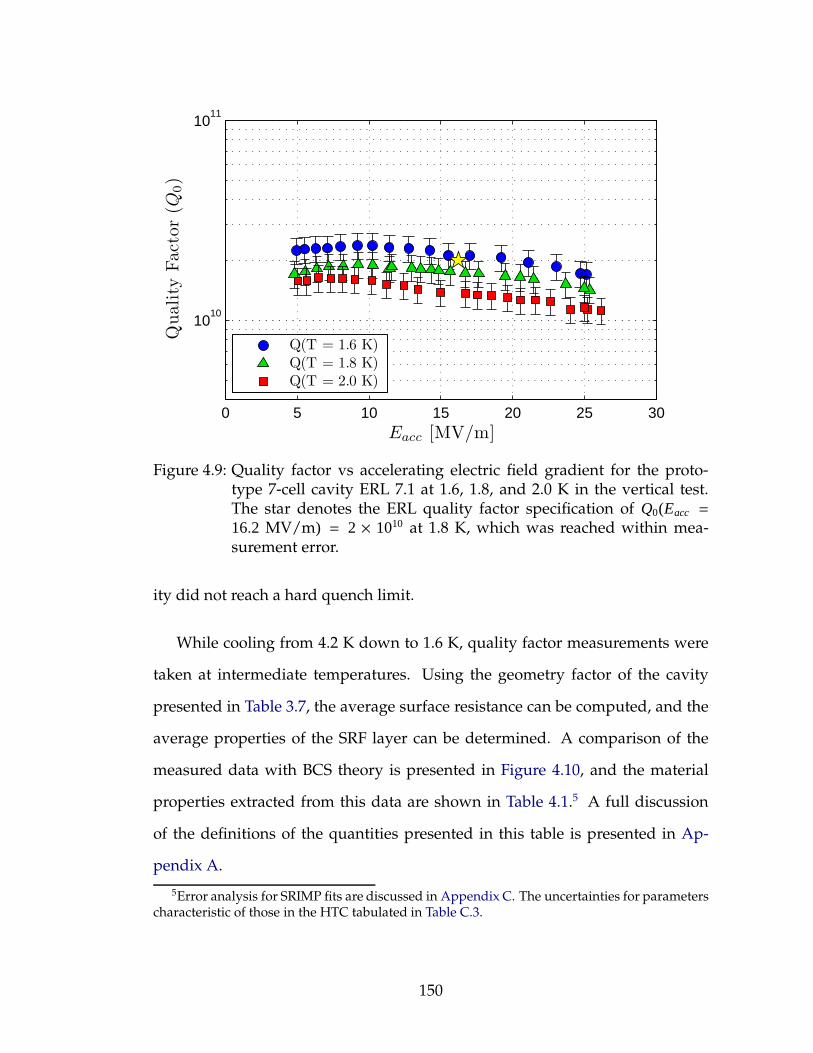
0 5 10 15 20 25 30
1010
1011
Quality
Fact
or
(Q0)
Eacc [MV/m]
Q(T = 1.6 K)Q(T = 1.8 K)Q(T = 2.0 K)
Figure 4.9: Quality factor vs accelerating electric field gradient for the proto-type 7-cell cavity ERL 7.1 at 1.6, 1.8, and 2.0 K in the vertical test.The star denotes the ERL quality factor specification of Q0(Eacc =
16.2 MV/m) = 2 × 10¹⁰ at 1.8 K, which was reached within mea-surement error.
ity did not reach a hard quench limit.
While cooling from 4.2 K down to 1.6 K, quality factor measurements were
taken at intermediate temperatures. Using the geometry factor of the cavity
presented in Table 3.7, the average surface resistance can be computed, and the
average properties of the SRF layer can be determined. A comparison of the
measured data with BCS theory is presented in Figure 4.10, and the material
properties extracted from this data are shown in Table 4.1.5 A full discussion
of the definitions of the quantities presented in this table is presented in Ap-
pendix A.
5Error analysis for SRIMP fits are discussed in Appendix C. The uncertainties for parameterscharacteristic of those in the HTC tabulated in Table C.3.
150

1.5 2 2.5 3 3.5 4 4.510
−8
10−7
10−6
Temperature [K]
Surf
ace
Res
ista
nce
[Ω]
BCS Theory + Residual ResistanceERL7.1 Vertical Test Measurement
Figure 4.10: Surface resistance vs temperature for the vertical test of the proto-type 7-cell cavity between 4.2 and 1.6 K. The material parametersfor this fit are presented in Table 4.1. (Can be compared with a laterresult in Figure 4.15.)
The quality factor measured at the proposed operating temperature of 1.8 K
and gradient of 16.2 MV/m was slightly lower than the design specification,
but was consistent within measurement uncertainty, so deemed successful. The
prototype qualifications continued to the next stage: Testing in a horizontal cry-
omodule.
4.3.2 Horizontal Test Cryomodule Program
The horizontal test cryomodule (HTC) program seeks to demonstrate that
the prototype cavity meets the fundamental mode design specification of
Q0(T=1.8 K) = 2×10¹⁰ at 16.2 MV/m, in a fully outfitted cavity, without deleteri-
151
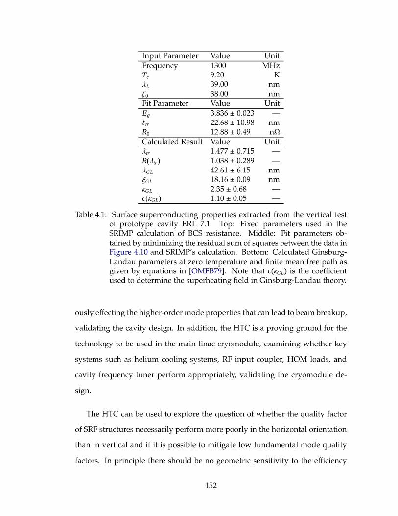
Input Parameter Value UnitFrequency 1300 MHzTc 9.20 KλL 39.00 nmξ0 38.00 nmFit Parameter Value UnitEg 3.836 ± 0.023 —ℓtr 22.68 ± 10.98 nmR0 12.88 ± 0.49 nΩCalculated Result Value Unitλtr 1.477 ± 0.715 —R(λtr) 1.038 ± 0.289 —λGL 42.61 ± 6.15 nmξGL 18.16 ± 0.09 nmκGL 2.35 ± 0.68 —c(κGL) 1.10 ± 0.05 —
Table 4.1: Surface superconducting properties extracted from the vertical testof prototype cavity ERL 7.1. Top: Fixed parameters used in theSRIMP calculation of BCS resistance. Middle: Fit parameters ob-tained by minimizing the residual sum of squares between the data inFigure 4.10 and SRIMP’s calculation. Bottom: Calculated Ginsburg-Landau parameters at zero temperature and finite mean free path asgiven by equations in [OMFB79]. Note that c(κGL) is the coefficientused to determine the superheating field in Ginsburg-Landau theory.
ously effecting the higher-order mode properties that can lead to beam breakup,
validating the cavity design. In addition, the HTC is a proving ground for the
technology to be used in the main linac cryomodule, examining whether key
systems such as helium cooling systems, RF input coupler, HOM loads, and
cavity frequency tuner perform appropriately, validating the cryomodule de-
sign.
The HTC can be used to explore the question of whether the quality factor
of SRF structures necessarily perform more poorly in the horizontal orientation
than in vertical and if it is possible to mitigate low fundamental mode quality
factors. In principle there should be no geometric sensitivity to the efficiency
152
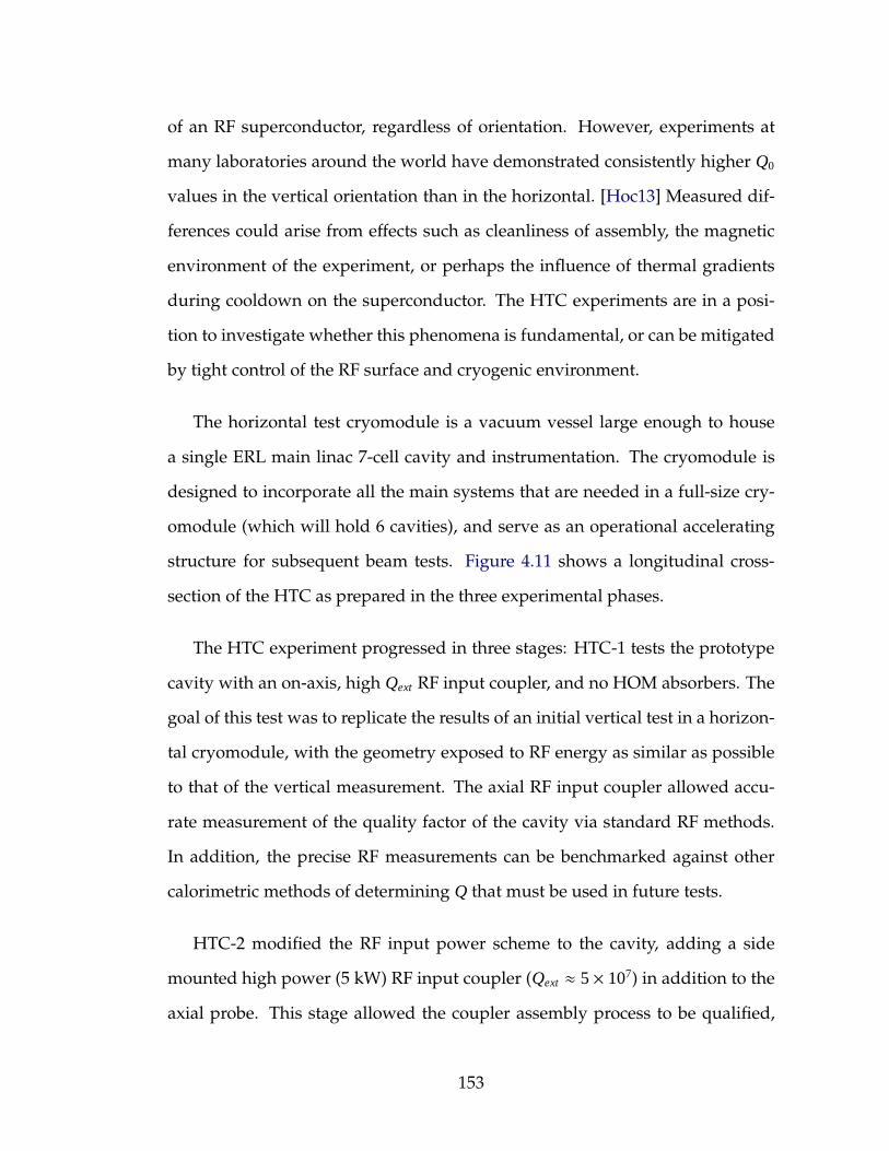
of an RF superconductor, regardless of orientation. However, experiments at
many laboratories around the world have demonstrated consistently higher Q0
values in the vertical orientation than in the horizontal. [Hoc13] Measured dif-
ferences could arise from effects such as cleanliness of assembly, the magnetic
environment of the experiment, or perhaps the influence of thermal gradients
during cooldown on the superconductor. The HTC experiments are in a posi-
tion to investigate whether this phenomena is fundamental, or can be mitigated
by tight control of the RF surface and cryogenic environment.
The horizontal test cryomodule is a vacuum vessel large enough to house
a single ERL main linac 7-cell cavity and instrumentation. The cryomodule is
designed to incorporate all the main systems that are needed in a full-size cry-
omodule (which will hold 6 cavities), and serve as an operational accelerating
structure for subsequent beam tests. Figure 4.11 shows a longitudinal cross-
section of the HTC as prepared in the three experimental phases.
The HTC experiment progressed in three stages: HTC-1 tests the prototype
cavity with an on-axis, high Qext RF input coupler, and no HOM absorbers. The
goal of this test was to replicate the results of an initial vertical test in a horizon-
tal cryomodule, with the geometry exposed to RF energy as similar as possible
to that of the vertical measurement. The axial RF input coupler allowed accu-
rate measurement of the quality factor of the cavity via standard RF methods.
In addition, the precise RF measurements can be benchmarked against other
calorimetric methods of determining Q that must be used in future tests.
HTC-2 modified the RF input power scheme to the cavity, adding a side
mounted high power (5 kW) RF input coupler (Qext ≈ 5× 10⁷) in addition to the
axial probe. This stage allowed the coupler assembly process to be qualified,
153
Figure 4.11: Longitudinal cross-sections of the HTC configuration in various ex-perimental phases. Top: Instrumentation in HTC-1 and -2. Themain difference is that HTC-2 incorporated a side-mounted highpower RF coupler. Bottom: HTC-3 including the beamline HOMabsorbing loads.
as well as preliminary investigations into the coupling between the high power
coupler and higher-order modes.
HTC-3 reconfigures the assembly, removing the axial power coupler and
adding two broadband beamline HOM absorbers–one on each end of the cav-
ity. Meeting gradient and quality factor specifications in this final test would
154
demonstrate the feasibility of all the main systems needed to fabricate a full
main linac ERL cryomodule.
Success in the HTC experimental program would demonstrate the viabil-
ity of the technology required for the Cornell ERL, and provide evidence that
all higher-order modes are strongly damped so that the linac would be able to
support current in excess of 100 mA through the linac.
4.3.3 HTC-1
Horizontal Installation
Following the vertical test, a helium jacket was welded to the outside of the
cavity. Before welding, six Cernox temperature sensors were permanently fixed
to the outer cavity surface. The sensors were located on the top and bottom of
each end cell, and the top and bottom of the center cell. During the welding
process, the interior remained under vacuum to preserve the cleanliness of the
SRF surface. Network analyzer measurements before and after attaching the he-
lium jacket indicated that the stress of welding did not change the fundamental
mode resonance frequency and field profile of the cavity.
After welding the helium jacket to the cavity, the cavity was high-pressure
rinsed, and an axial probe with Qext ∼ 9 × 10¹⁰ to the fundamental mode was
installed at one end of the cavity. The Qext of the coupler was chosen to be higher
than in the vertical test to help reduce RF losses on the coupler which could
introduce errors into the measurement of the cavity’s intrinsic quality factor.
A side mounted field probe, with Qext ∼ 3 × 10¹¹ to the fundamental mode,
155
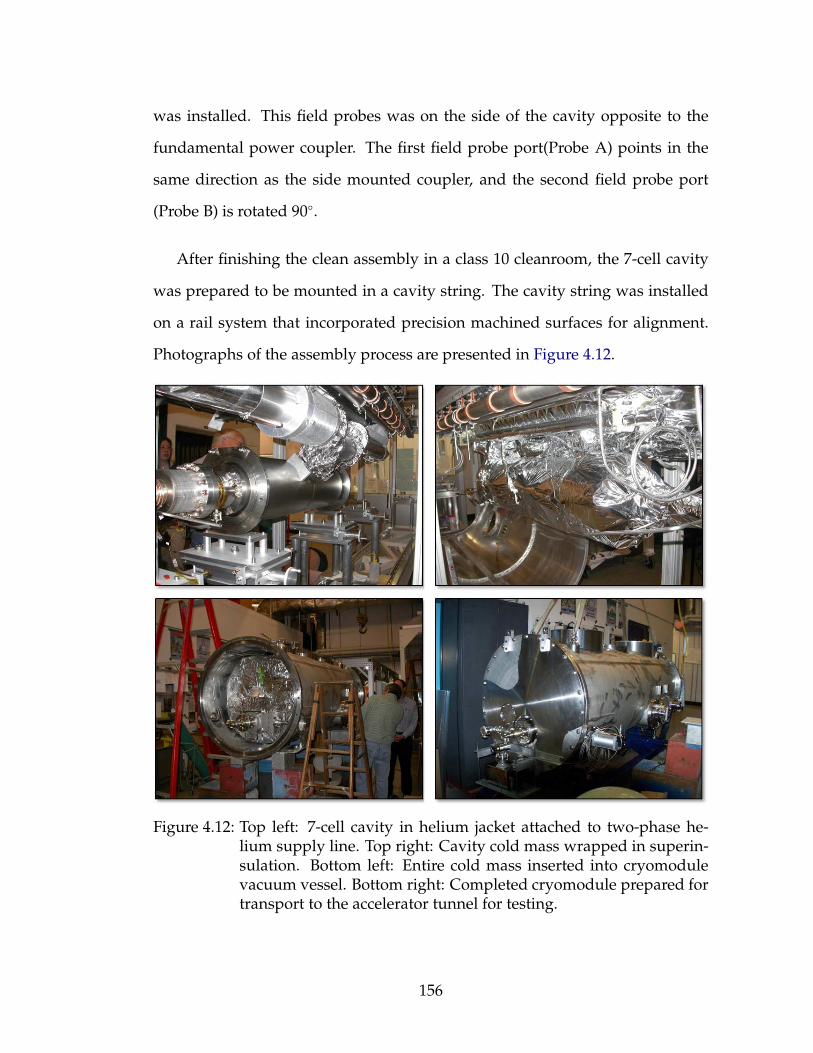
was installed. This field probes was on the side of the cavity opposite to the
fundamental power coupler. The first field probe port(Probe A) points in the
same direction as the side mounted coupler, and the second field probe port
(Probe B) is rotated 90.
After finishing the clean assembly in a class 10 cleanroom, the 7-cell cavity
was prepared to be mounted in a cavity string. The cavity string was installed
on a rail system that incorporated precision machined surfaces for alignment.
Photographs of the assembly process are presented in Figure 4.12.
Figure 4.12: Top left: 7-cell cavity in helium jacket attached to two-phase he-lium supply line. Top right: Cavity cold mass wrapped in superin-sulation. Bottom left: Entire cold mass inserted into cryomodulevacuum vessel. Bottom right: Completed cryomodule prepared fortransport to the accelerator tunnel for testing.
156
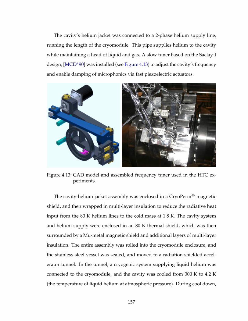
The cavity’s helium jacket was connected to a 2-phase helium supply line,
running the length of the cryomodule. This pipe supplies helium to the cavity
while maintaining a head of liquid and gas. A slow tuner based on the Saclay-I
design, [MCD+90] was installed (see Figure 4.13) to adjust the cavity’s frequency
and enable damping of microphonics via fast piezoelectric actuators.
Figure 4.13: CAD model and assembled frequency tuner used in the HTC ex-periments.
The cavity-helium jacket assembly was enclosed in a CryoPerm R© magnetic
shield, and then wrapped in multi-layer insulation to reduce the radiative heat
input from the 80 K helium lines to the cold mass at 1.8 K. The cavity system
and helium supply were enclosed in an 80 K thermal shield, which was then
surrounded by a Mu-metal magnetic shield and additional layers of multi-layer
insulation. The entire assembly was rolled into the cryomodule enclosure, and
the stainless steel vessel was sealed, and moved to a radiation shielded accel-
erator tunnel. In the tunnel, a cryogenic system supplying liquid helium was
connected to the cryomodule, and the cavity was cooled from 300 K to 4.2 K
(the temperature of liquid helium at atmospheric pressure). During cool down,
157
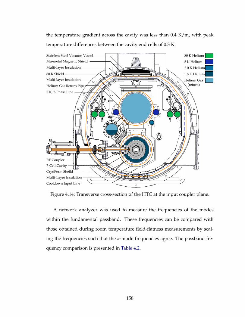
the temperature gradient across the cavity was less than 0.4 K/m, with peak
temperature differences between the cavity end cells of 0.3 K.
Figure 4.14: Transverse cross-section of the HTC at the input coupler plane.
A network analyzer was used to measure the frequencies of the modes
within the fundamental passband. These frequencies can be compared with
those obtained during room temperature field-flatness measurements by scal-
ing the frequencies such that the π-mode frequencies agree. The passband fre-
quency comparison is presented in Table 4.2.
158

Mode Scaled Bead-Pull HTC-1 Network Analyzer ∆ f[MHz] [MHz] [kHz]
1π/7 1274.772 1274.726 46.22π/7 1278.234 1278.197 36.63π/7 1283.573 1283.544 29.44π/7 1289.209 1289.194 14.65π/7 1294.801 1294.792 9.296π/7 1298.449 1298.451 -1.607π/7 1299.879 1299.879 0.000
Table 4.2: Frequencies of the modes in the fundamental passband from thescaled field-flatness measurement and in HTC-1. The slight discrep-ancy in values can either arise from small shape changes during thewelding of the helium vessel to the cavity or from handling. The cor-respondence between the two frequency measurements suggest thecavity field flatness was preserved in HTC-1.
Quality Factor Determination
For HTC-1, the intrinsic quality factor of the cavity was measured both with
standard RF methods and calorimetrically. Benchmarking the calorimetric
methods is essential since later measurements will use RF couplers with rel-
atively low Qext and so will not be able to accurately Q0 via RF methods. The
calorimetric methods relied on the dissipated power in the cavity walls acting as
a heater, and measuring either the rate of change of the helium level or helium
gas exhaust to determine the power input into the helium bath.
Fundamental Mode Qualification via RF Measurements
The quality factor of the cavity was characterized using an analog phase-locked
loop system to perform RF measurements as illustrated in Figure 4.15. The
phase-lock loop system tracks the cavity’s resonant frequency by using a phase
detector to produce a voltage proportional to the difference between the cavity’s
159
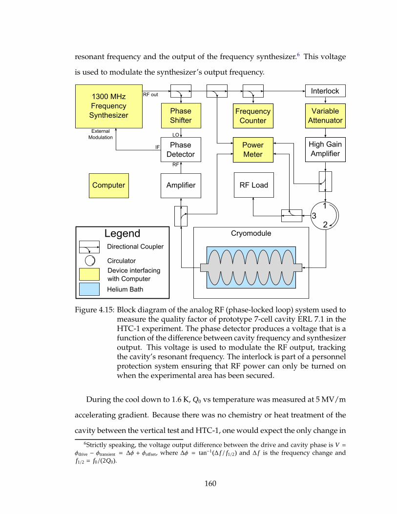
resonant frequency and the output of the frequency synthesizer.6 This voltage
is used to modulate the synthesizer’s output frequency.
1300 MHz
Frequency
Synthesizer
Interlock
High Gain
Amplifier
1
23
RF Load
Power
Meter
Amplifier
Phase
Detector
Frequency
Counter
Cryomodule
Phase
Shifter
Computer
Variable
Attenuator
Legend
Circulator
Directional Coupler
Device interfacing
with Computer
Helium Bath
RF out
External
Modulation
RF
LO
IF
Figure 4.15: Block diagram of the analog RF (phase-locked loop) system used tomeasure the quality factor of prototype 7-cell cavity ERL 7.1 in theHTC-1 experiment. The phase detector produces a voltage that is afunction of the difference between cavity frequency and synthesizeroutput. This voltage is used to modulate the RF output, trackingthe cavity’s resonant frequency. The interlock is part of a personnelprotection system ensuring that RF power can only be turned onwhen the experimental area has been secured.
During the cool down to 1.6 K, Q0 vs temperature was measured at 5 MV/m
accelerating gradient. Because there was no chemistry or heat treatment of the
cavity between the vertical test and HTC-1, one would expect the only change in
6Strictly speaking, the voltage output difference between the drive and cavity phase is V =φdrive − φtransient = ∆φ + φoffset, where ∆φ = tan−1(∆ f / f1/2) and ∆ f is the frequency change andf1/2 = f0/(2Q0).
160
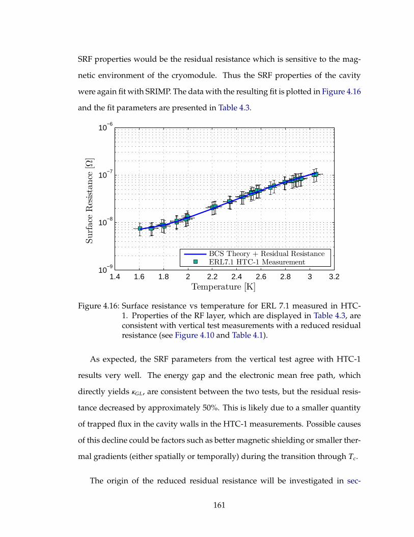
SRF properties would be the residual resistance which is sensitive to the mag-
netic environment of the cryomodule. Thus the SRF properties of the cavity
were again fit with SRIMP. The data with the resulting fit is plotted in Figure 4.16
and the fit parameters are presented in Table 4.3.
1.4 1.6 1.8 2 2.2 2.4 2.6 2.8 3 3.210
−9
10−8
10−7
10−6
Temperature [K]
Surf
ace
Res
ista
nce
[Ω]
BCS Theory + Residual ResistanceERL7.1 HTC-1 Measurement
Figure 4.16: Surface resistance vs temperature for ERL 7.1 measured in HTC-1. Properties of the RF layer, which are displayed in Table 4.3, areconsistent with vertical test measurements with a reduced residualresistance (see Figure 4.10 and Table 4.1).
As expected, the SRF parameters from the vertical test agree with HTC-1
results very well. The energy gap and the electronic mean free path, which
directly yields κGL, are consistent between the two tests, but the residual resis-
tance decreased by approximately 50%. This is likely due to a smaller quantity
of trapped flux in the cavity walls in the HTC-1 measurements. Possible causes
of this decline could be factors such as better magnetic shielding or smaller ther-
mal gradients (either spatially or temporally) during the transition through Tc.
The origin of the reduced residual resistance will be investigated in sec-
161
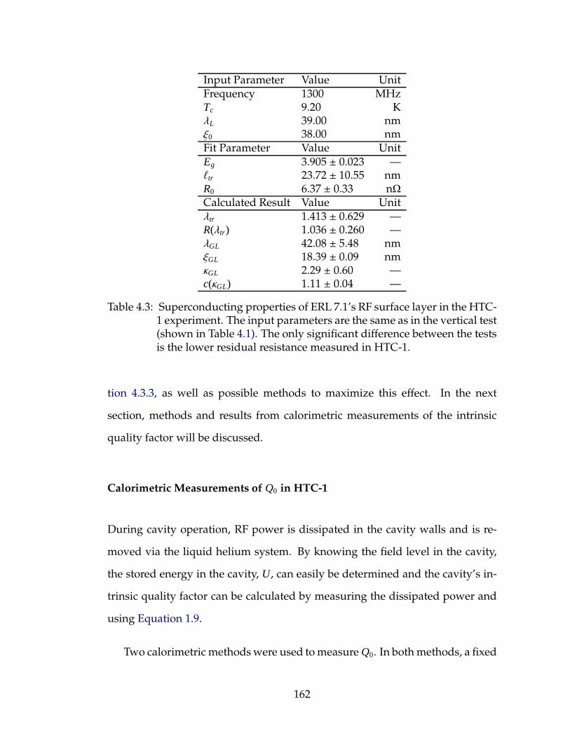
Input Parameter Value UnitFrequency 1300 MHzTc 9.20 KλL 39.00 nmξ0 38.00 nmFit Parameter Value UnitEg 3.905 ± 0.023 —ℓtr 23.72 ± 10.55 nmR0 6.37 ± 0.33 nΩCalculated Result Value Unitλtr 1.413 ± 0.629 —R(λtr) 1.036 ± 0.260 —λGL 42.08 ± 5.48 nmξGL 18.39 ± 0.09 nmκGL 2.29 ± 0.60 —c(κGL) 1.11 ± 0.04 —
Table 4.3: Superconducting properties of ERL 7.1’s RF surface layer in the HTC-1 experiment. The input parameters are the same as in the vertical test(shown in Table 4.1). The only significant difference between the testsis the lower residual resistance measured in HTC-1.
tion 4.3.3, as well as possible methods to maximize this effect. In the next
section, methods and results from calorimetric measurements of the intrinsic
quality factor will be discussed.
Calorimetric Measurements of Q0 in HTC-1
During cavity operation, RF power is dissipated in the cavity walls and is re-
moved via the liquid helium system. By knowing the field level in the cavity,
the stored energy in the cavity, U, can easily be determined and the cavity’s in-
trinsic quality factor can be calculated by measuring the dissipated power and
using Equation 1.9.
Two calorimetric methods were used to measure Q0. In both methods, a fixed
162
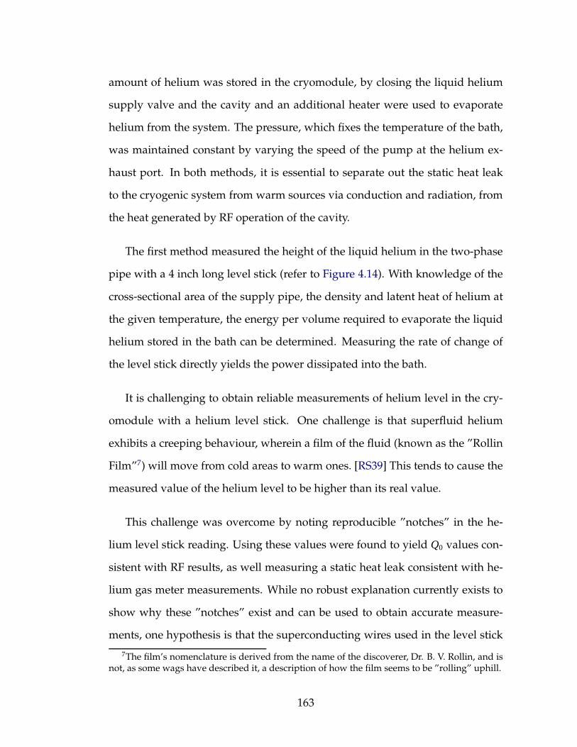
amount of helium was stored in the cryomodule, by closing the liquid helium
supply valve and the cavity and an additional heater were used to evaporate
helium from the system. The pressure, which fixes the temperature of the bath,
was maintained constant by varying the speed of the pump at the helium ex-
haust port. In both methods, it is essential to separate out the static heat leak
to the cryogenic system from warm sources via conduction and radiation, from
the heat generated by RF operation of the cavity.
The first method measured the height of the liquid helium in the two-phase
pipe with a 4 inch long level stick (refer to Figure 4.14). With knowledge of the
cross-sectional area of the supply pipe, the density and latent heat of helium at
the given temperature, the energy per volume required to evaporate the liquid
helium stored in the bath can be determined. Measuring the rate of change of
the level stick directly yields the power dissipated into the bath.
It is challenging to obtain reliable measurements of helium level in the cry-
omodule with a helium level stick. One challenge is that superfluid helium
exhibits a creeping behaviour, wherein a film of the fluid (known as the ”Rollin
Film”7) will move from cold areas to warm ones. [RS39] This tends to cause the
measured value of the helium level to be higher than its real value.
This challenge was overcome by noting reproducible ”notches” in the he-
lium level stick reading. Using these values were found to yield Q0 values con-
sistent with RF results, as well measuring a static heat leak consistent with he-
lium gas meter measurements. While no robust explanation currently exists to
show why these ”notches” exist and can be used to obtain accurate measure-
ments, one hypothesis is that the superconducting wires used in the level stick
7The film’s nomenclature is derived from the name of the discoverer, Dr. B. V. Rollin, and isnot, as some wags have described it, a description of how the film seems to be ”rolling” uphill.
163

3.5 3.6 3.7 3.8 3.9 4 4.1
x 104
5
10
15
20
25
30
35
40
45
Late
nt
Ener
gy
[kJ]
Time [s]
Figure 4.17: Latent energy in the two-phase supply pipe as a function of time,measured by a helium level stick. The blue points represent thelevel stick data, green circles mark the ”notches” which occur atreproducible energy points, and the black dashed line shows thedetermined boil-off rate of the helium. During this measurement,there was no RF power in the cavity, and a heater attached to thehelium supply pipe was run at 5.5 W. The level stick measurementyields dissipated bath power of 6.4± 0.3 W. The difference betweenreading and measurement is due to a heat input present regardlessof operating condition, known as the static heat load.
have irregular cross-sectional area, leading to certain places that the film pools
when its weight becomes too large to support a vertical film. A plot showing
typical notches and how they were used to measure power dissipation is pre-
sented in Figure 4.17.
The second calorimetric method measured the mass flow of helium ex-
hausted from the cryogenic pumps. Using the specific heat, density, and ther-
mal integrals of helium from cryogenic temperatures to room temperature, the
energy per unit volume stored in the gas can be calculated. The volumetric rate
164
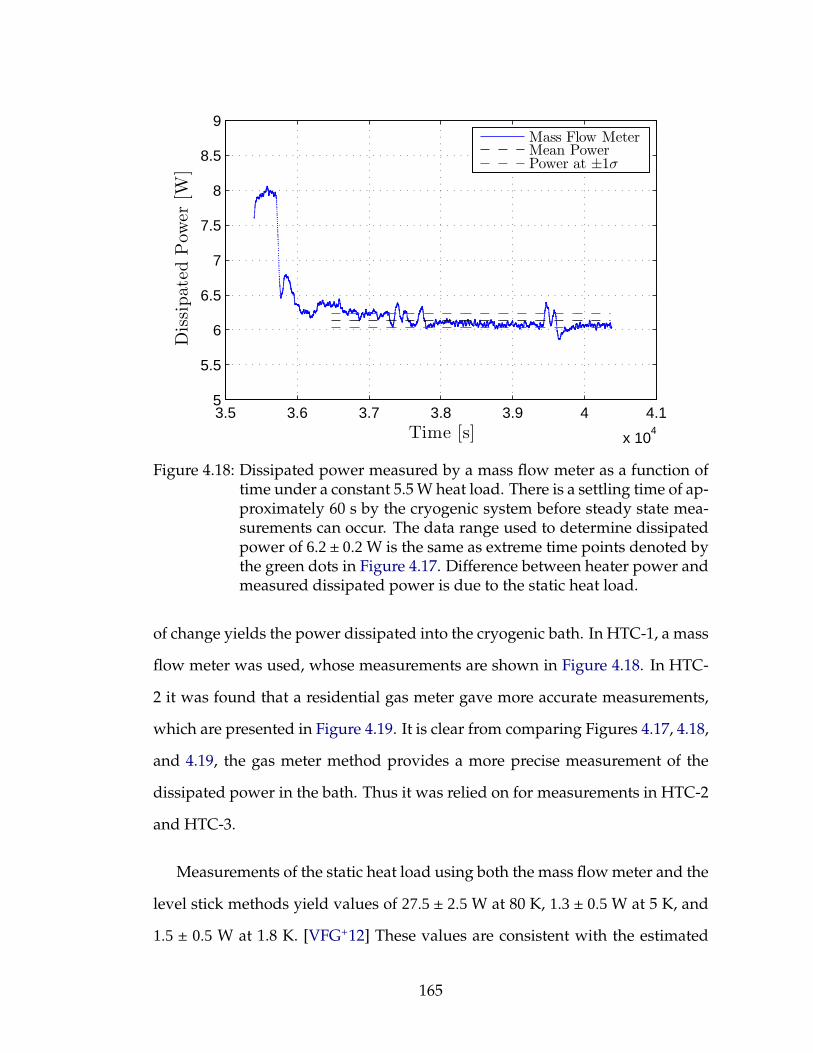
3.5 3.6 3.7 3.8 3.9 4 4.1
x 104
5
5.5
6
6.5
7
7.5
8
8.5
9
Time [s]
Dis
sipate
dP
ower
[W]
Mass Flow MeterMean PowerPower at ±1σ
Figure 4.18: Dissipated power measured by a mass flow meter as a function oftime under a constant 5.5 W heat load. There is a settling time of ap-proximately 60 s by the cryogenic system before steady state mea-surements can occur. The data range used to determine dissipatedpower of 6.2± 0.2 W is the same as extreme time points denoted bythe green dots in Figure 4.17. Difference between heater power andmeasured dissipated power is due to the static heat load.
of change yields the power dissipated into the cryogenic bath. In HTC-1, a mass
flow meter was used, whose measurements are shown in Figure 4.18. In HTC-
2 it was found that a residential gas meter gave more accurate measurements,
which are presented in Figure 4.19. It is clear from comparing Figures 4.17, 4.18,
and 4.19, the gas meter method provides a more precise measurement of the
dissipated power in the bath. Thus it was relied on for measurements in HTC-2
and HTC-3.
Measurements of the static heat load using both the mass flow meter and the
level stick methods yield values of 27.5± 2.5 W at 80 K, 1.3± 0.5 W at 5 K, and
1.5 ± 0.5 W at 1.8 K. [VFG+12] These values are consistent with the estimated
165

6.4 6.45 6.5 6.55 6.6 6.65 6.7 6.75 6.8
x 104
85
90
95
100
105
110
115
Ener
gy
[kJ]
Time [s]
Figure 4.19: Energy measured by the gas meter as a function of time under aconstant 4.5 W heat load. The blue points represent the gas meterdata, and the red line is a least squares fit yielding the dissipatedpower of 5.4 ± 0.1 W. Difference between heater power and mea-sured dissipated power is due to the static heat load.
static heat leak at 1.8 K of ∼2 W, validating the cryomodule design.
Calorimetric measurements of the quality factor of the cavity at 1.8 K are
compared with RF measurements in Figure 4.20. These measurements were
made by filling the helium supply pipe ∼70% full, and closing the helium input
valve. First, a heater at a constant power and the cavity at a fixed field level
was used to boil off helium in the cryomodule until only ∼15% remained in the
pipe. The helium was refilled, and the measurement redone with only the heater
on. The power difference between the two runs is interpreted as the dissipated
power from the cavity and can be used in Equation 1.9 to directly yield Q0.
The quality factors measured by both RF and calorimetric methods were con-
166

0 5 10 15 20
1010
1011
Quality
Fact
or
Eacc [MV/m]
RF MethodMass Flow MethodHelium Level Drop Method
Figure 4.20: Q0 vs Eacc measurement at 1.8 K for the initial cool down of HTC-1.RF measurements are compared with the two calorimetric methodsof measuring Q0 and shown to be consistent.
sistent with one another. The large uncertainty in the calorimetric method is due
to the uncertainty in the static heat load, and from the fact that determining Q0
relies on a difference measurement. The consistency between the two methods
demonstrated that calorimetric measurements are reliable, an essential result
for subsequent HTC experiments.
Thermal Cycling Effects on Quality Factor
The initial Q0 measurements at 16.2 MV/m showed 1.8 K values slightly exceed-
ing the 2× 10¹⁰ design specification, arising entirely from a lower residual resis-
tance. Previous work has shown that the Meissner effect is incomplete in pure
Nb samples, which contributes to residual resistance through trapped magnetic
flux, [AKK12] so the high level of magnetic shielding in the HTC gives high
167
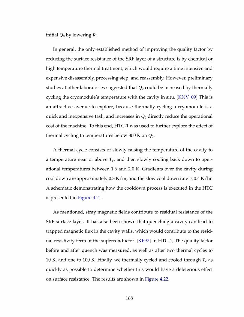
initial Q0 by lowering R0.
In general, the only established method of improving the quality factor by
reducing the surface resistance of the SRF layer of a structure is by chemical or
high temperature thermal treatment, which would require a time intensive and
expensive disassembly, processing step, and reassembly. However, preliminary
studies at other laboratories suggested that Q0 could be increased by thermally
cycling the cryomodule’s temperature with the cavity in situ. [KNV+09] This is
an attractive avenue to explore, because thermally cycling a cryomodule is a
quick and inexpensive task, and increases in Q0 directly reduce the operational
cost of the machine. To this end, HTC-1 was used to further explore the effect of
thermal cycling to temperatures below 300 K on Q0.
A thermal cycle consists of slowly raising the temperature of the cavity to
a temperature near or above Tc, and then slowly cooling back down to oper-
ational temperatures between 1.6 and 2.0 K. Gradients over the cavity during
cool down are approximately 0.3 K/m, and the slow cool down rate is 0.4 K/hr.
A schematic demonstrating how the cooldown process is executed in the HTC
is presented in Figure 4.21.
As mentioned, stray magnetic fields contribute to residual resistance of the
SRF surface layer. It has also been shown that quenching a cavity can lead to
trapped magnetic flux in the cavity walls, which would contribute to the resid-
ual resistivity term of the superconductor. [KP97] In HTC-1, The quality factor
before and after quench was measured, as well as after two thermal cycles to
10 K, and one to 100 K. Finally, we thermally cycled and cooled through Tc as
quickly as possible to determine whether this would have a deleterious effect
on surface resistance. The results are shown in Figure 4.22.
168

Figure 4.21: Schematic of the cooldown process in the HTC. Helium gas flowssymmetrically around the cavity from two inputs at the bottom ofthe helium jacket. Helium is exhausted through a chimney abovethe center of the cavity to the two-phase line and helium gas returnpipe where it is recovered.
The Q0 vs Eacc measurements did not show degradation between the initial
cool down and after quenching the cavity several times. After the first cycle to
10 K, the cavity’s quality factor improved by ∼20%, and a second low tempera-
ture cycle to 12 K yielded an additional ∼20% improvement in Q0.
It was hypothesized that due to a slow leak in the cavity’s vacuum sys-
tem, there could be gasses condensed on the RF surface, contributing to the
residual resistance. Since most gasses are not mobile below 77 K, the cavity
was thermally cycled to 100 K and retested. The Q0 achieved in this measure-
ment was ∼50% higher than that obtained in the initial cool down, reaching
Q0 = (3.0 ± 0.3) × 1010 at 1.8 K and 16.2 MV/m. Within experimental certainty,
this result was consistent with the post 12 K cooldown. A subsequent fast cool
down did not degrade the quality factor.
These results demonstrate that it is possible to improve the quality factor of
a cavity simply by cycling through Tc several times maintaining small thermal
169
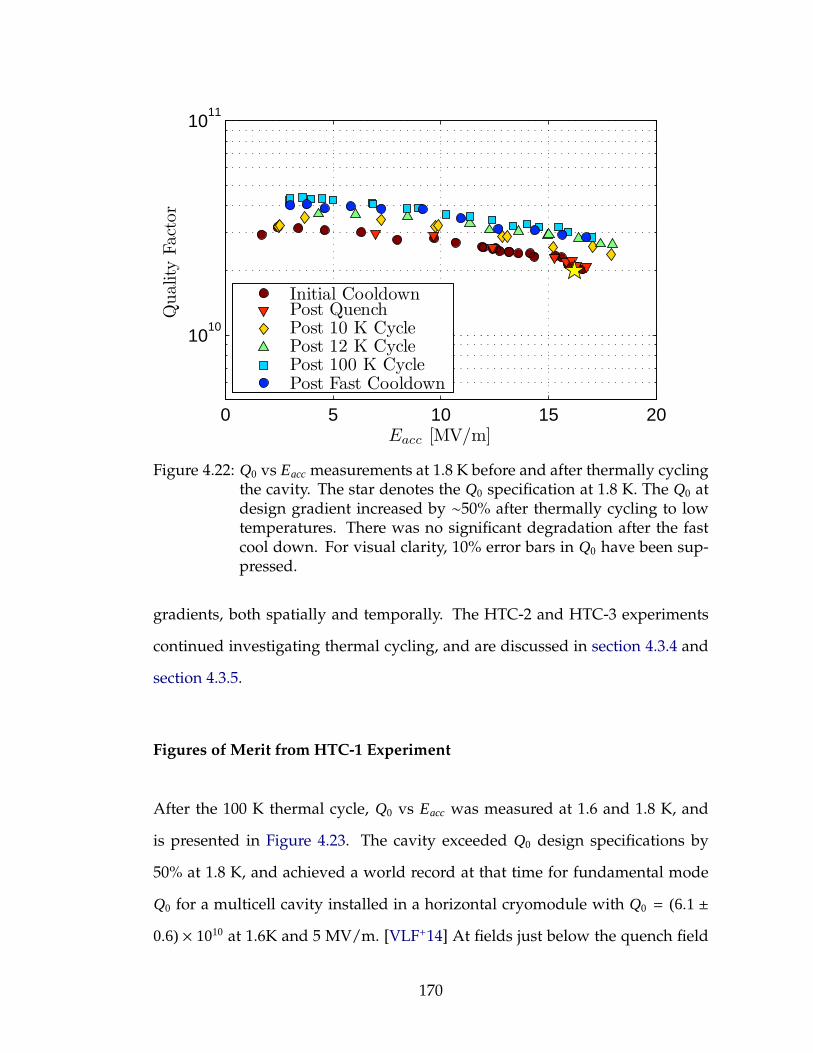
0 5 10 15 20
1010
1011
Eacc [MV/m]
Quality
Fact
or
Initial CooldownPost QuenchPost 10 K CyclePost 12 K CyclePost 100 K CyclePost Fast Cooldown
Figure 4.22: Q0 vs Eacc measurements at 1.8 K before and after thermally cyclingthe cavity. The star denotes the Q0 specification at 1.8 K. The Q0 atdesign gradient increased by ∼50% after thermally cycling to lowtemperatures. There was no significant degradation after the fastcool down. For visual clarity, 10% error bars in Q0 have been sup-pressed.
gradients, both spatially and temporally. The HTC-2 and HTC-3 experiments
continued investigating thermal cycling, and are discussed in section 4.3.4 and
section 4.3.5.
Figures of Merit from HTC-1 Experiment
After the 100 K thermal cycle, Q0 vs Eacc was measured at 1.6 and 1.8 K, and
is presented in Figure 4.23. The cavity exceeded Q0 design specifications by
50% at 1.8 K, and achieved a world record at that time for fundamental mode
Q0 for a multicell cavity installed in a horizontal cryomodule with Q0 = (6.1 ±
0.6)× 1010 at 1.6K and 5 MV/m. [VLF+14] At fields just below the quench field
170
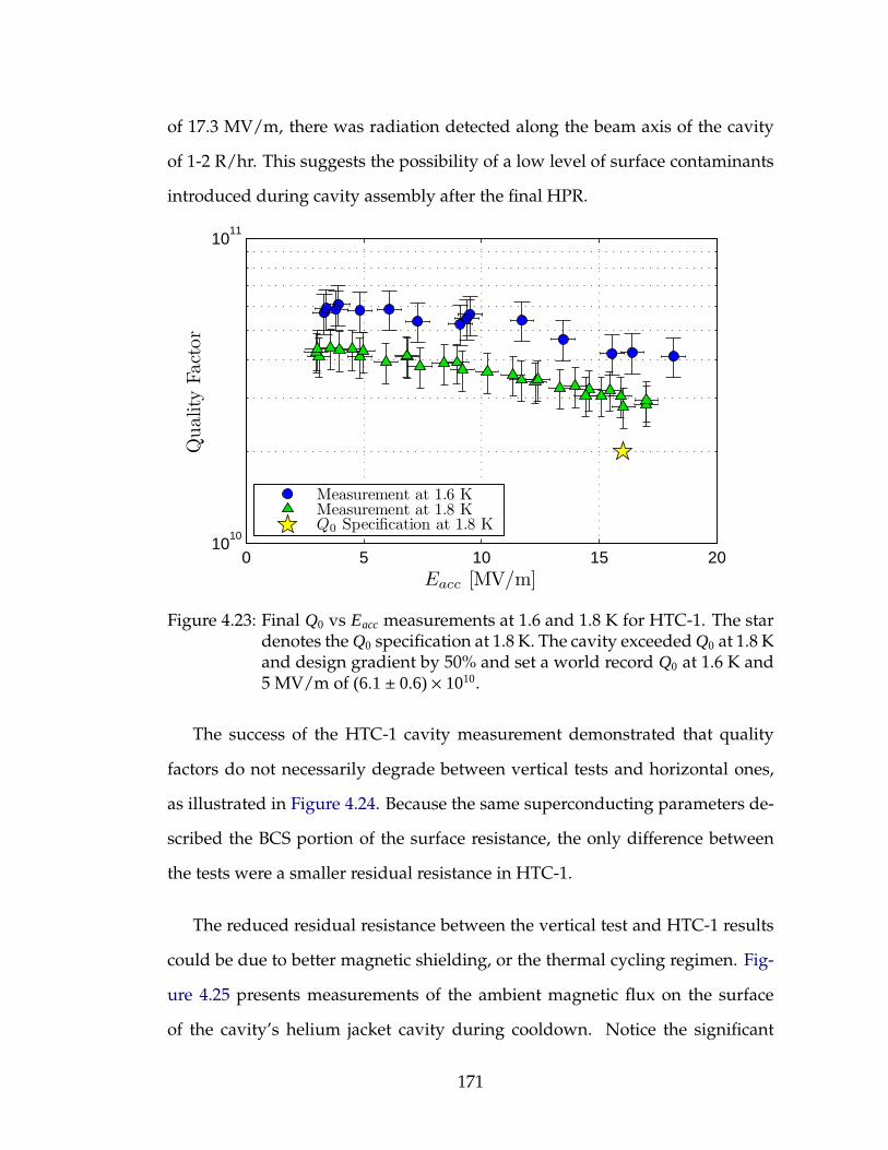
of 17.3 MV/m, there was radiation detected along the beam axis of the cavity
of 1-2 R/hr. This suggests the possibility of a low level of surface contaminants
introduced during cavity assembly after the final HPR.
0 5 10 15 2010
10
1011
Quality
Fact
or
Eacc [MV/m]
Measurement at 1.6 KMeasurement at 1.8 KQ0 Specification at 1.8 K
Figure 4.23: Final Q0 vs Eacc measurements at 1.6 and 1.8 K for HTC-1. The stardenotes the Q0 specification at 1.8 K. The cavity exceeded Q0 at 1.8 Kand design gradient by 50% and set a world record Q0 at 1.6 K and5 MV/m of (6.1± 0.6)× 1010.
The success of the HTC-1 cavity measurement demonstrated that quality
factors do not necessarily degrade between vertical tests and horizontal ones,
as illustrated in Figure 4.24. Because the same superconducting parameters de-
scribed the BCS portion of the surface resistance, the only difference between
the tests were a smaller residual resistance in HTC-1.
The reduced residual resistance between the vertical test and HTC-1 results
could be due to better magnetic shielding, or the thermal cycling regimen. Fig-
ure 4.25 presents measurements of the ambient magnetic flux on the surface
of the cavity’s helium jacket cavity during cooldown. Notice the significant
171
0 5 10 15 20 25 3010
10
1011
Quality
Fact
or
Eacc [MV/m]
VerticalHTC-1
Figure 4.24: Comparison of Q0 vs Eacc between vertical test and HTC-1 at 1.8 K.Measurements in HTC-1 show much higher Q0, due to lower resid-ual resistance, than in the vertical test even though no surface treat-ment was done between measurements.
changes in the ambient magnetic flux changes during cooldown.
Ambient magnetic flux can pin to impurity sites in a superconductor, trap-
ping magnetic flux and increasing residual resistance. [VBB+92] The authors
of [VBB+92] present a phenomenological result applicable to SRF cavities relat-
ing the residual resistance, R0, the ambient magnetic field, Bext, the upper critical
field of the superconductor, Bc2, and the normal state resistance, Rn, according
to
R0 = Rn ·Bext
Bc2
. (4.1)
Reasonable values for Rn of 1.3 GHz niobium resonators are between 1.5 and
1.8 mΩ. [PKH98] Generally speaking, Bc2 is not known for a superconducting
cavity, but it is reasonable to assume Bc2 = 400mT (see Table 2.2). The ambient
172

Time
Tem
per
atu
re[K
]
12:00 15:00 18:00 21:00 00:000
10
20
30
40
50
60
70
80
−0.3
−0.2
−0.1
0
0.1
0.2
0.3
0.4
0.5
Magnet
icF
lux
[µT
]
L. Beam Tube TempR. Beam Tube TempFlux Gate Probe
Figure 4.25: Fluxgate magnetometer measurement during HTC cooldown.Temperature sensors on each beam tube recorded the temperatureduring cooldown. The light blue region highlights a time period inwhich the helium valve was set incorrectly. The light green regionmarks the time that the field reversed polarity, requiring reconfigu-ration of the analog inputs, which was completed just before 21:00hours.
flux during the transition through Tc in the HTC experiments was 0.2 µT, corre-
sponding to residual resistance due to trapped flux of (0.8±0.2) nΩ. This can be
compared with ambient flux of 5− 10µT in the vertical test (R0 between 1.8 and
4.5 nΩ). Application of Equation 4.1 with the measured magnetic flux does not
account for the entire residual resistance observed in the vertical and horizontal
tests.
The sign change of the measured flux during cooldown hints that there may
be thermal currents8 in the cryomodule during cooldown. Currents inside the
8The Seebeck effect describes how temperature gradients influence the local current densityvia J = σ(−∇V − S∇T ), where S is the thermopower of the material. [Ash76]
173
structure can produce magnetic fields, but since the fluxgate probe is outside
the helium vessel, the fields measured by the magnetometer may not be repre-
sentative of the the local magnetic flux at the surface of the cavity.
While the HTC is optimized to achieve small thermal gradients during
cooldown, non-zero thermal gradient induced currents may contribute to the
cavity’s residual resistance in addition to the ambient flux inside the cryomod-
ule. One hypothesis is that thermal currents may be reduced during successive
thermal cycles, leading to the reduction in R0. This effect is further studied in
HTC-2.
The next stage of experiments investigated whether the same performance
could be repeated for the more complicated assembly, needed in an actual ac-
celerator environment.
4.3.4 HTC-2
Following the success of HTC-1, the cryomodule was disassembled, and the
cavity received an HPR to remove any residual surface contaminants. The cav-
ity was then cleanly reassembled with the same procedure as described in sec-
tion 4.3.3.
Instead of the axial coupler used in the vertical test and HTC-1, for HTC-2
a high power side mounted coupler was installed on the cavity (refer to Fig-
ure 4.11 and Figure 4.14 for high power coupler location in the HTC). It can
couple 5 kW of power to the cavity and has a fixed nominal external quality
factor, Qext , of 6.5× 10⁷. [BBB+11] The coupler consists of two main parts: a cold
174
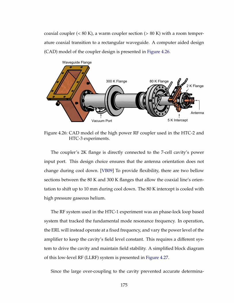
coaxial coupler (< 80 K), a warm coupler section (> 80 K) with a room temper-
ature coaxial transition to a rectangular waveguide. A computer aided design
(CAD) model of the coupler design is presented in Figure 4.26.
Antenna
2 K Flange
5 K Intercept
80 K Flange300 K Flange
Waveguide Flange
Vacuum Port
Figure 4.26: CAD model of the high power RF coupler used in the HTC-2 andHTC-3 experiments.
The coupler’s 2K flange is directly connected to the 7-cell cavity’s power
input port. This design choice ensures that the antenna orientation does not
change during cool down. [VB09] To provide flexibility, there are two bellow
sections between the 80 K and 300 K flanges that allow the coaxial line’s orien-
tation to shift up to 10 mm during cool down. The 80 K intercept is cooled with
high pressure gaseous helium.
The RF system used in the HTC-1 experiment was an phase-lock loop based
system that tracked the fundamental mode resonance frequency. In operation,
the ERL will instead operate at a fixed frequency, and vary the power level of the
amplifier to keep the cavity’s field level constant. This requires a different sys-
tem to drive the cavity and maintain field stability. A simplified block diagram
of this low-level RF (LLRF) system is presented in Figure 4.27.
Since the large over-coupling to the cavity prevented accurate determina-
175
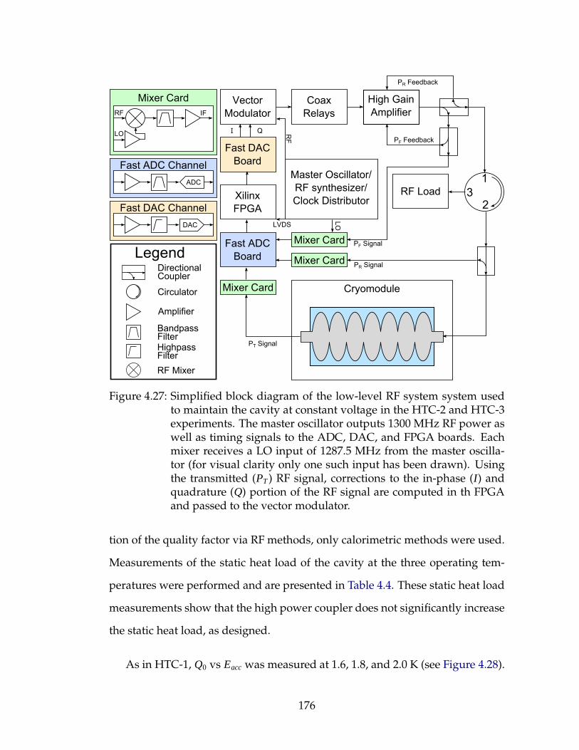
Master Oscillator/
RF synthesizer/
Clock Distributor
Vector
Modulator
Coax
Relays
High Gain
Amplifier
Cryomodule
1
23RF LoadXilinx
FPGA
Fast ADC
Board
Fast DAC
Board
Mixer Card
Mixer Card
Mixer Card
I Q
PF Feedback
PR Feedback
PR Signal
PF Signal
PT Signal
Fast ADC Channel
ADC
RF
LOLVDS
Mixer Card
LO
RF IF
Fast DAC Channel
DAC
Legend
Circulator
DirectionalCoupler
Amplifier
BandpassFilterHighpassFilter
RF Mixer
Figure 4.27: Simplified block diagram of the low-level RF system system usedto maintain the cavity at constant voltage in the HTC-2 and HTC-3experiments. The master oscillator outputs 1300 MHz RF power aswell as timing signals to the ADC, DAC, and FPGA boards. Eachmixer receives a LO input of 1287.5 MHz from the master oscilla-tor (for visual clarity only one such input has been drawn). Usingthe transmitted (PT ) RF signal, corrections to the in-phase (I) andquadrature (Q) portion of the RF signal are computed in th FPGAand passed to the vector modulator.
tion of the quality factor via RF methods, only calorimetric methods were used.
Measurements of the static heat load of the cavity at the three operating tem-
peratures were performed and are presented in Table 4.4. These static heat load
measurements show that the high power coupler does not significantly increase
the static heat load, as designed.
As in HTC-1, Q0 vs Eacc was measured at 1.6, 1.8, and 2.0 K (see Figure 4.28).
176
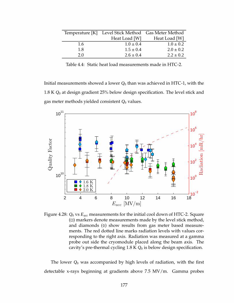
Temperature [K] Level Stick Method Gas Meter MethodHeat Load [W] Heat Load [W]
1.6 1.0± 0.4 1.0± 0.21.8 1.5± 0.4 2.0± 0.22.0 2.6± 0.4 2.2± 0.2
Table 4.4: Static heat load measurements made in HTC-2.
Initial measurements showed a lower Q0 than was achieved in HTC-1, with the
1.8 K Q0 at design gradient 25% below design specification. The level stick and
gas meter methods yielded consistent Q0 values.
2 4 6 8 10 12 14 16 18
1010
1011
Eacc [MV/m]
Quality
Fact
or
1.6 K1.8 K2.0 K
10−2
100
102
104
106
108
Radia
tion
[mR
/hr]
Figure 4.28: Q0 vs Eacc measurements for the initial cool down of HTC-2. Square() markers denote measurements made by the level stick method,and diamonds (♦) show results from gas meter based measure-ments. The red dotted line marks radiation levels with values cor-responding to the right axis. Radiation was measured at a gammaprobe out side the cryomodule placed along the beam axis. Thecavity’s pre-thermal cycling 1.8 K Q0 is below design specification.
The lower Q0 was accompanied by high levels of radiation, with the first
detectable x-rays beginning at gradients above 7.5 MV/m. Gamma probes
177

mounted at each end of the cryomodule along the beam tube measured x-ray
doses above 2 kR/hr, and a neutron detector measured 3 × 10³ neutrons/hr at
the coupler end of the cryomodule. Because the highest radiation was highest
at the gamma probe closest to the high power coupler, it is likely that source
of electrons was from the end cell far from the coupler. Electrons were likely
field emitted from the cell surface and were accelerated through the structure,
striking the wall of the cryomodule and releasing x-rays and neutrons. Gen-
erally, electrons arise from small conducting dust particles that serve as a field
emitters, which comes from a sub-optimal assembly procedure.
Thermal Cycling Effects on Quality Factor
As in HTC-1, investigations into thermal cycling’s effect on Q0 was continued
during the HTC-2 experiment. Since HTC-1 had already demonstrated that
thermal cycling can be beneficial, the next step was to determine the tempera-
ture at which benefits first begin. Initially, two thermal cycles were performed to
low temperatures (15 K). Benefits in HTC-1 were observed from both low tem-
perature and high temperature cycles, so following the low temperature thermal
cycles two additional high temperature thermal cycles were performed, the first
to 100 K and the second to 300 K. Finally a thermal cycle to a temperature below
Tc was performed, to test whether flux can tunnel out of the superconducting
bulk, an idea which has been tested in samples, [VKK13] but never confirmed
in a superconducting cavity.
The results of thermal cycling on the cavity’s Q0 (measured at 1.8 K) are
presented in Figure 4.29. In this plot, data obtained with the level stick and gas
meter have been averaged. The most benefit was obtained after the first thermal
178
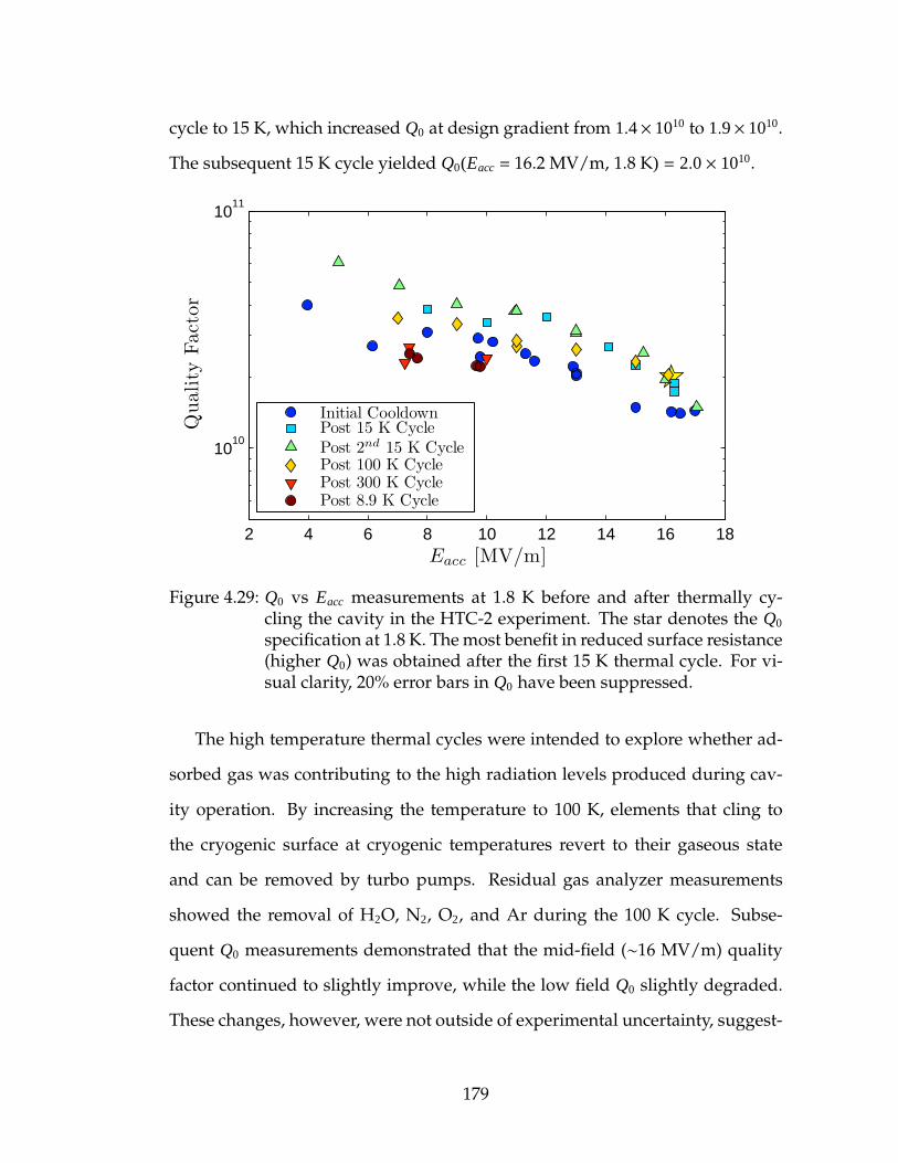
cycle to 15 K, which increased Q0 at design gradient from 1.4× 10¹⁰ to 1.9× 10¹⁰.
The subsequent 15 K cycle yielded Q0(Eacc = 16.2 MV/m, 1.8 K) = 2.0× 10¹⁰.
2 4 6 8 10 12 14 16 18
1010
1011
Eacc [MV/m]
Quality
Fact
or
Initial CooldownPost 15 K CyclePost 2nd 15 K CyclePost 100 K CyclePost 300 K CyclePost 8.9 K Cycle
Figure 4.29: Q0 vs Eacc measurements at 1.8 K before and after thermally cy-cling the cavity in the HTC-2 experiment. The star denotes the Q0
specification at 1.8 K. The most benefit in reduced surface resistance(higher Q0) was obtained after the first 15 K thermal cycle. For vi-sual clarity, 20% error bars in Q0 have been suppressed.
The high temperature thermal cycles were intended to explore whether ad-
sorbed gas was contributing to the high radiation levels produced during cav-
ity operation. By increasing the temperature to 100 K, elements that cling to
the cryogenic surface at cryogenic temperatures revert to their gaseous state
and can be removed by turbo pumps. Residual gas analyzer measurements
showed the removal of H2O, N2, O2, and Ar during the 100 K cycle. Subse-
quent Q0 measurements demonstrated that the mid-field (∼16 MV/m) quality
factor continued to slightly improve, while the low field Q0 slightly degraded.
These changes, however, were not outside of experimental uncertainty, suggest-
179
ing that residual gasses play no significant role in the thermal cycling effect.
A complete warmup to 300 K was performed to see if the thermal cycle ben-
efits were cumulative, or if they had to be redone for each cool down from
room temperature. Unfortunately, during the cool down process there was a
small vacuum leak causing the cavity pressure to increase from 1 × 10⁻⁷ Torr
to 2 × 10⁻⁴ Torr. Additional pumping was added to the cavity vacuum space,
and the cycle continued. At 1.8 K, the cavity performance was consistent with
the measurements during the initial cool down, though high radiation levels
prevented operating the cavity at accelerating gradients above 10 MV/m, im-
plying the benefit of thermal cycling is lost when the cavity is returned to room
temperature.
Since the cavity performance after the 300 K cool down was similar to the
initial cool down, the effect of the maximum temperature reached during a
cycle could be directly compared. In this case, a cycle to below 9 K was per-
formed, wherein the cavity temperature was maintained between 8 and 8.9 K
for 40 minutes, and then returned to 1.8 K. With this cycle, no improvement
in the quality factor was observed. This suggests that thermal cycling benefits
occur when reaching maximum temperatures above Tc but well below room
temperature. [VEF+13]
Possible explanations for the reduction in residual resistance include remov-
ing adsorbed gasses from the surface of the conductor or thermoelectric effects
changing the amount of trapped flux in the superconductor.
If gasses were the source of the residual resistance, increasing temperatures
to about 15 K is not a high enough temperature for them to become mobile and
180
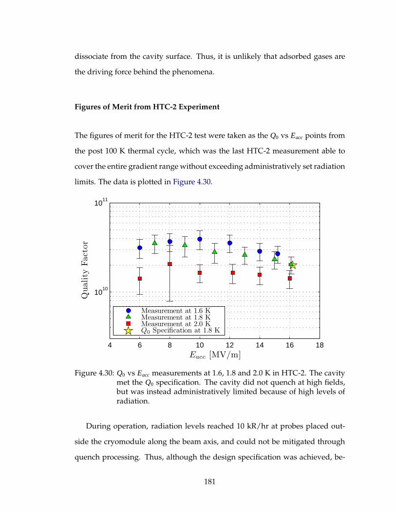
dissociate from the cavity surface. Thus, it is unlikely that adsorbed gases are
the driving force behind the phenomena.
Figures of Merit from HTC-2 Experiment
The figures of merit for the HTC-2 test were taken as the Q0 vs Eacc points from
the post 100 K thermal cycle, which was the last HTC-2 measurement able to
cover the entire gradient range without exceeding administratively set radiation
limits. The data is plotted in Figure 4.30.
4 6 8 10 12 14 16 18
1010
1011
Quality
Fact
or
Eacc [MV/m]
Measurement at 1.6 KMeasurement at 1.8 KMeasurement at 2.0 KQ0 Specification at 1.8 K
Figure 4.30: Q0 vs Eacc measurements at 1.6, 1.8 and 2.0 K in HTC-2. The cavitymet the Q0 specification. The cavity did not quench at high fields,but was instead administratively limited because of high levels ofradiation.
During operation, radiation levels reached 10 kR/hr at probes placed out-
side the cryomodule along the beam axis, and could not be mitigated through
quench processing. Thus, although the design specification was achieved, be-
181
fore proceeding with the fully equipped cryomodule in HTC-3, chemical pro-
cessing was required to remove the source of field emission in the end cell far
from the input power coupler.
4.3.5 HTC-3
Following the HTC-2 experiment, the cryomodule was disassembled and the
cavity received a 5 µm BCP with the intent of removing the source of field emis-
sion from the cavity surface followed by a 120C heat treatment for 48 hr and
a single HF rinse, oxide regrowth step. [RGBO13] The cavity was then high
pressure rinsed and assembled into the cryomodule along with two beam-line
higher-order mode loads (see bottom of Figure 4.11 for reference).
The part of the HOM loads that absorbs RF energy is made of a SiC loaded
ceramic9, [Coo06] which is brazed to a tungsten fixture that attaches directly to
the cavity flange. The HOM loads serve not only to damp higher-order modes,
but also as bellows connecting the main linac cavities (see Figure 4.31). The
absorbers are designed to extract up to 200 W of HOM power for frequencies
up to 150 GHz. [ECH+13]
The loads have two points that are thermally anchored. The first is the 5 K
intercept right after the stainless steel bellows. Because the HOM load is directly
connected to the cavity flange, and the cavity will operate at 1.8 K, anchoring
the HOM load at 5 K helps to reduce the conduction losses to the liquid helium
bath. The second anchor point is the cooling tube apparatus (nominally at 80 K)
that removes the HOM power.
9It is a commercially available material with the trade name of Coorstek R© SC-35.
182
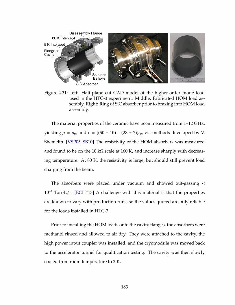
Figure 4.31: Left: Half-plane cut CAD model of the higher-order mode loadused in the HTC-3 experiment. Middle: Fabricated HOM load as-sembly. Right: Ring of SiC absorber prior to brazing into HOM loadassembly.
The material properties of the ceramic have been measured from 1–12 GHz,
yielding µ = µ0, and ǫ = [(50 ± 10)− (28± 7)]ǫ0, via methods developed by V.
Shemelin. [VSP05, SB10] The resistivity of the HOM absorbers was measured
and found to be on the 10 kΩ scale at 160 K, and increase sharply with decreas-
ing temperature. At 80 K, the resistivity is large, but should still prevent load
charging from the beam.
The absorbers were placed under vacuum and showed out-gassing <
10−7 Torr·L/s. [ECH+13] A challenge with this material is that the properties
are known to vary with production runs, so the values quoted are only reliable
for the loads installed in HTC-3.
Prior to installing the HOM loads onto the cavity flanges, the absorbers were
methanol rinsed and allowed to air dry. They were attached to the cavity, the
high power input coupler was installed, and the cryomodule was moved back
to the accelerator tunnel for qualification testing. The cavity was then slowly
cooled from room temperature to 2 K.
183
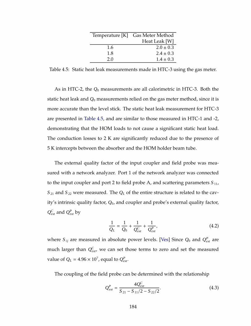
Temperature [K] Gas Meter MethodHeat Leak [W]
1.6 2.0± 0.31.8 2.4± 0.32.0 1.4± 0.3
Table 4.5: Static heat leak measurements made in HTC-3 using the gas meter.
As in HTC-2, the Q0 measurements are all calorimetric in HTC-3. Both the
static heat leak and Q0 measurements relied on the gas meter method, since it is
more accurate than the level stick. The static heat leak measurement for HTC-3
are presented in Table 4.5, and are similar to those measured in HTC-1 and -2,
demonstrating that the HOM loads to not cause a significant static heat load.
The conduction losses to 2 K are significantly reduced due to the presence of
5 K intercepts between the absorber and the HOM holder beam tube.
The external quality factor of the input coupler and field probe was mea-
sured with a network analyzer. Port 1 of the network analyzer was connected
to the input coupler and port 2 to field probe A, and scattering parameters S 11,
S 21 and S 22 were measured. The QL of the entire structure is related to the cav-
ity’s intrinsic quality factor, Q0, and coupler and probe’s external quality factor,
QCext and QP
ext by
1QL=
1Q0+
1
QCext
+1
QPext
, (4.2)
where S i j are measured in absolute power levels. [Ves] Since Q0 and QPext are
much larger than QCext , we can set those terms to zero and set the measured
value of QL = 4.96× 10⁷, equal to QPext .
The coupling of the field probe can be determined with the relationship
QPext =
4QCext
S 21− S 11/2− S 22/2. (4.3)
184
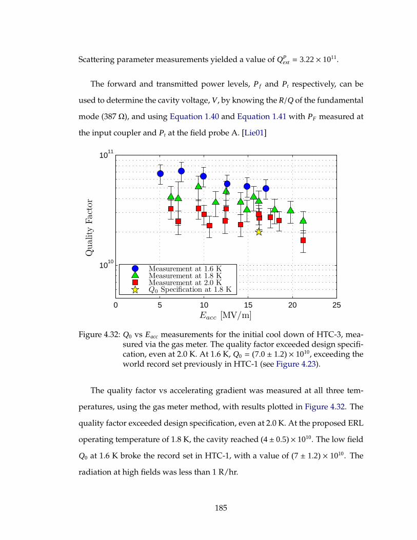
Scattering parameter measurements yielded a value of QPext = 3.22× 10¹¹.
The forward and transmitted power levels, P f and Pt respectively, can be
used to determine the cavity voltage, V , by knowing the R/Q of the fundamental
mode (387 Ω), and using Equation 1.40 and Equation 1.41 with PF measured at
the input coupler and Pt at the field probe A. [Lie01]
0 5 10 15 20 25
1010
1011
Eacc [MV/m]
Quality
Fact
or
Measurement at 1.6 KMeasurement at 1.8 KMeasurement at 2.0 KQ0 Specification at 1.8 K
Figure 4.32: Q0 vs Eacc measurements for the initial cool down of HTC-3, mea-sured via the gas meter. The quality factor exceeded design specifi-cation, even at 2.0 K. At 1.6 K, Q0 = (7.0± 1.2)× 1010, exceeding theworld record set previously in HTC-1 (see Figure 4.23).
The quality factor vs accelerating gradient was measured at all three tem-
peratures, using the gas meter method, with results plotted in Figure 4.32. The
quality factor exceeded design specification, even at 2.0 K. At the proposed ERL
operating temperature of 1.8 K, the cavity reached (4± 0.5)× 1010. The low field
Q0 at 1.6 K broke the record set in HTC-1, with a value of (7 ± 1.2) × 1010. The
radiation at high fields was less than 1 R/hr.
185
The Q0 of the fully outfitted cavity in HTC-3 exceeded design specification
by a factor of 2, meaning the cavity’s surface has extremely small surface resis-
tance. At 1.6 K, the BCS resistance is small, and Rs is dominated by residual
resistance. The lowest surface resistance achieved in the initial cool down was
only ∼4 nΩ which is already better than the residual resistance obtained after
thermal cycling in HTC-1 of roughly 6 nΩ (see Table 4.3).
One difference in surface preparation between HTC-1 and HTC-3 is the HF
rinse after 120C heat treatment. It is known that the heat treatment lowers the
BCS component of resistance while increasing the residual resistance. The HF
rinse helps to reduce the residual resistance, resulting in very high Q0 structures.
[RGBO13] Thus whether thermal cycling could reduce the residual resistance
below this already very low value is an interesting question.
Thermal Cycling Effects on Quality Factor
Due to time constraints, only a single thermal cycle could be performed dur-
ing the HTC-3 experiment. Since HTC-2 demonstrated no benefit by thermally
cycling to below 9 K, and both HTC-1 and HTC-2 showed benefit from a 15 K
thermal cycle, it was decided to perform the thermal cycle to a maximum tem-
perature just above Tc.
The thermal cycle was performed, holding the cavity temperature above Tc
for about 30 minutes, and reaching a peak temperature of 10.1 K, as shown in
Figure 4.33. During cool down, the peak-to-peak temperature difference across
the cavity was 0.2 K, giving a maximum thermal gradient of 0.25 K/m. As
shown in as the cavity transitioned through Tc, the temperature was decreasing
186
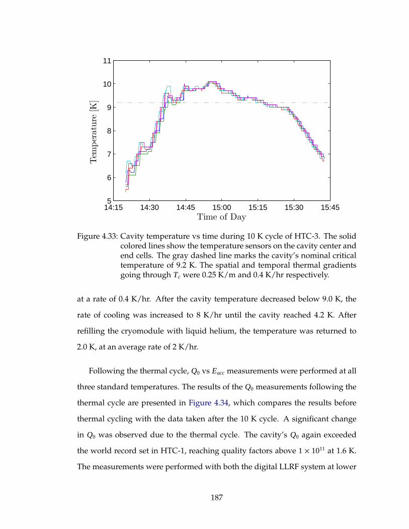
14:15 14:30 14:45 15:00 15:15 15:30 15:455
6
7
8
9
10
11
Time of Day
Tem
per
atu
re[K
]
Figure 4.33: Cavity temperature vs time during 10 K cycle of HTC-3. The solidcolored lines show the temperature sensors on the cavity center andend cells. The gray dashed line marks the cavity’s nominal criticaltemperature of 9.2 K. The spatial and temporal thermal gradientsgoing through Tc were 0.25 K/m and 0.4 K/hr respectively.
at a rate of 0.4 K/hr. After the cavity temperature decreased below 9.0 K, the
rate of cooling was increased to 8 K/hr until the cavity reached 4.2 K. After
refilling the cryomodule with liquid helium, the temperature was returned to
2.0 K, at an average rate of 2 K/hr.
Following the thermal cycle, Q0 vs Eacc measurements were performed at all
three standard temperatures. The results of the Q0 measurements following the
thermal cycle are presented in Figure 4.34, which compares the results before
thermal cycling with the data taken after the 10 K cycle. A significant change
in Q0 was observed due to the thermal cycle. The cavity’s Q0 again exceeded
the world record set in HTC-1, reaching quality factors above 1 × 10¹¹ at 1.6 K.
The measurements were performed with both the digital LLRF system at lower
187
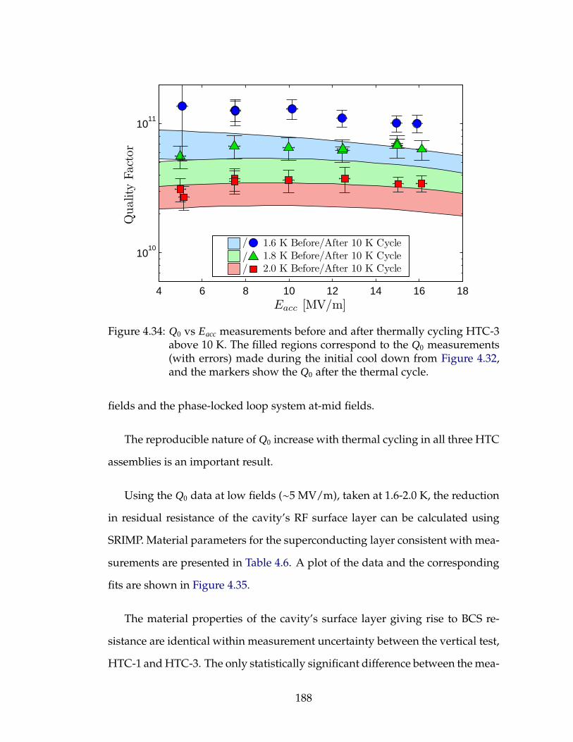
Quality
Fact
or
Eacc [MV/m]
/
//
4 6 8 10 12 14 16 18
1010
1011
1.6 K Before/After 10 K Cycle1.8 K Before/After 10 K Cycle2.0 K Before/After 10 K Cycle
Figure 4.34: Q0 vs Eacc measurements before and after thermally cycling HTC-3above 10 K. The filled regions correspond to the Q0 measurements(with errors) made during the initial cool down from Figure 4.32,and the markers show the Q0 after the thermal cycle.
fields and the phase-locked loop system at-mid fields.
The reproducible nature of Q0 increase with thermal cycling in all three HTC
assemblies is an important result.
Using the Q0 data at low fields (∼5 MV/m), taken at 1.6-2.0 K, the reduction
in residual resistance of the cavity’s RF surface layer can be calculated using
SRIMP. Material parameters for the superconducting layer consistent with mea-
surements are presented in Table 4.6. A plot of the data and the corresponding
fits are shown in Figure 4.35.
The material properties of the cavity’s surface layer giving rise to BCS re-
sistance are identical within measurement uncertainty between the vertical test,
HTC-1 and HTC-3. The only statistically significant difference between the mea-
188

Cool down: Initial Post 10 KInput Parameter Value Value UnitFrequency 1300 1300 MHzTc 9.20 9.20 KλL 39.00 39.00 nmξ0 38.00 38.00 nmFit Parameter Value Value UnitEg 3.887 ± 0.058 —ℓtr 24.74 ± 23.77 nmR0 3.20 ± 0.34 1.34 ± 0.14 nΩCalculated Result Value Value Unitλtr 1.355 ± 1.303 —R(λtr) 1.035 ± 0.557 —λGL 41.59 ± 11.51 nmξGL 18.61 ± 0.14 nmκGL 2.24 ± 1.24 —c(κGL) 1.11 ± 0.09 —
Table 4.6: Surface superconducting properties extracted from measurements ofERL 7.1 in the HTC-3 experiment. The same energy gap and mean freepath was used to fit both sets of data, allowing the residual resistanceto vary between runs.
surements arises from disparities in residual resistance. Though residual resis-
tances decreased in all measurements over thermal cycles, in HTC-3, the resid-
ual resistance decreased by about 66% from 3.2 nΩ to 1.3 nΩ after the 10 K ther-
mal cycle. This is a remarkable result when one considers that typical residual
resistances for cavities in cryomodules are between 5-15 nΩ. The fundamental
mode Q0 measurements of ERL 7.1 are the best ever achieved in a cryomodule.
Additional thermal cycling measurements would be interesting to perform,
unfortunately further thermal cycling investigations were not possible due to
limited laboratory resources.
189
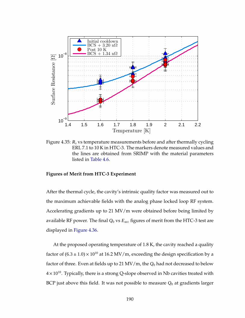
1.4 1.5 1.6 1.7 1.8 1.9 2 2.1 2.210
−9
10−8
Temperature [K]
Surf
ace
Res
ista
nce
[Ω]
Initial cooldownBCS + 3.20 nΩPost 10 KBCS + 1.34 nΩ
Figure 4.35: Rs vs temperature measurements before and after thermally cyclingERL 7.1 to 10 K in HTC-3. The markers denote measured values andthe lines are obtained from SRIMP with the material parameterslisted in Table 4.6.
Figures of Merit from HTC-3 Experiment
After the thermal cycle, the cavity’s intrinsic quality factor was measured out to
the maximum achievable fields with the analog phase locked loop RF system.
Accelerating gradients up to 21 MV/m were obtained before being limited by
available RF power. The final Q0 vs Eacc figures of merit from the HTC-3 test are
displayed in Figure 4.36.
At the proposed operating temperature of 1.8 K, the cavity reached a quality
factor of (6.3± 1.0)× 1010 at 16.2 MV/m, exceeding the design specification by a
factor of three. Even at fields up to 21 MV/m, the Q0 had not decreased to below
4×10¹⁰. Typically, there is a strong Q-slope observed in Nb cavities treated with
BCP just above this field. It was not possible to measure Q0 at gradients larger
190
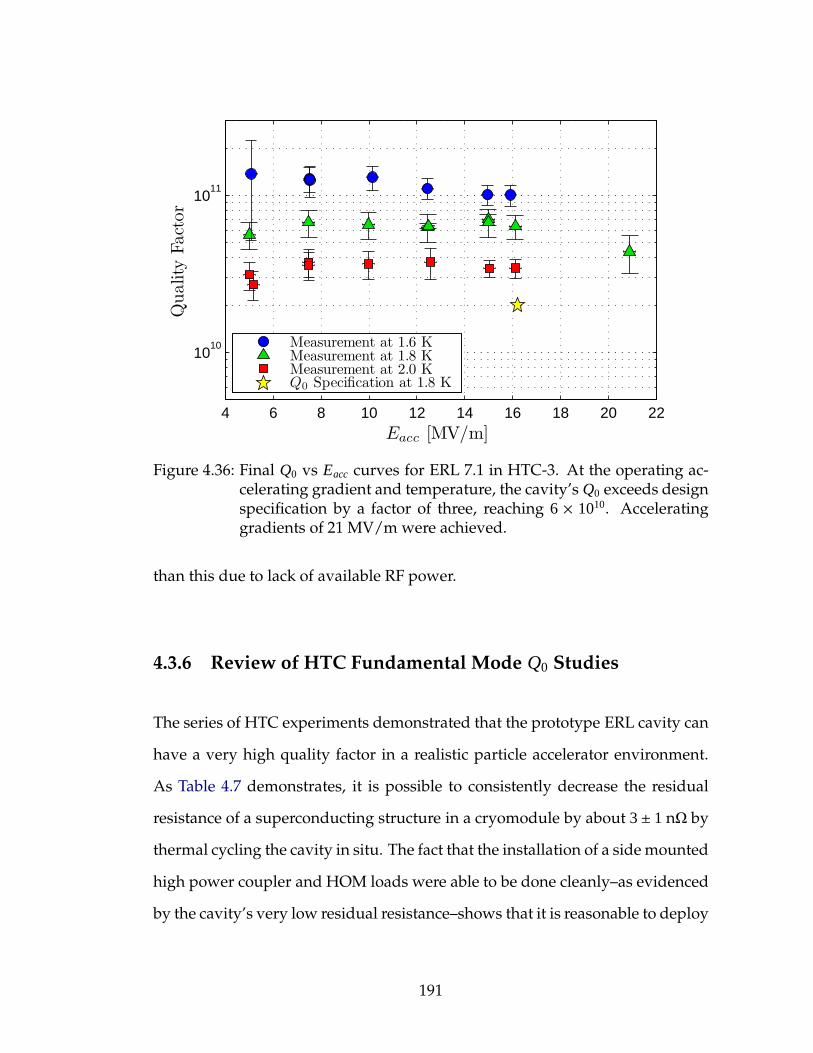
4 6 8 10 12 14 16 18 20 22
1010
1011
Eacc [MV/m]
Quality
Fact
or
Measurement at 1.6 KMeasurement at 1.8 KMeasurement at 2.0 KQ0 Specification at 1.8 K
Figure 4.36: Final Q0 vs Eacc curves for ERL 7.1 in HTC-3. At the operating ac-celerating gradient and temperature, the cavity’s Q0 exceeds designspecification by a factor of three, reaching 6 × 10¹⁰. Acceleratinggradients of 21 MV/m were achieved.
than this due to lack of available RF power.
4.3.6 Review of HTC Fundamental Mode Q0 Studies
The series of HTC experiments demonstrated that the prototype ERL cavity can
have a very high quality factor in a realistic particle accelerator environment.
As Table 4.7 demonstrates, it is possible to consistently decrease the residual
resistance of a superconducting structure in a cryomodule by about 3± 1 nΩ by
thermal cycling the cavity in situ. The fact that the installation of a side mounted
high power coupler and HOM loads were able to be done cleanly–as evidenced
by the cavity’s very low residual resistance–shows that it is reasonable to deploy
191
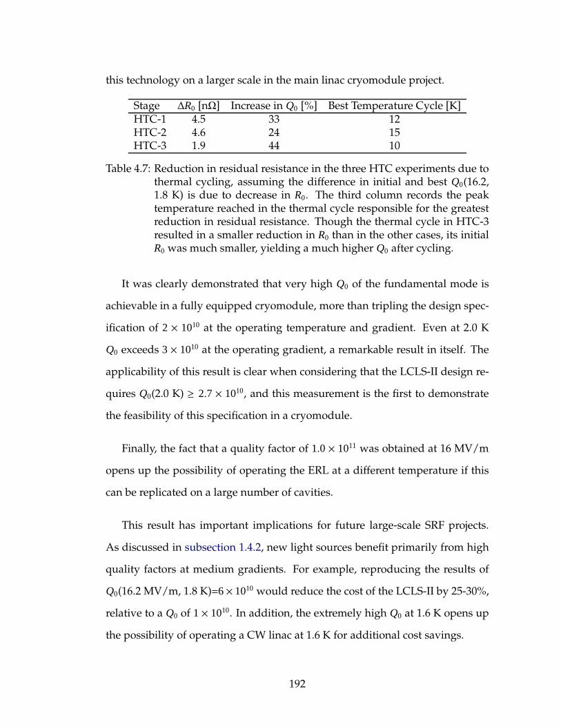
this technology on a larger scale in the main linac cryomodule project.
Stage ∆R0 [nΩ] Increase in Q0 [%] Best Temperature Cycle [K]HTC-1 4.5 33 12HTC-2 4.6 24 15HTC-3 1.9 44 10
Table 4.7: Reduction in residual resistance in the three HTC experiments due tothermal cycling, assuming the difference in initial and best Q0(16.2,1.8 K) is due to decrease in R0. The third column records the peaktemperature reached in the thermal cycle responsible for the greatestreduction in residual resistance. Though the thermal cycle in HTC-3resulted in a smaller reduction in R0 than in the other cases, its initialR0 was much smaller, yielding a much higher Q0 after cycling.
It was clearly demonstrated that very high Q0 of the fundamental mode is
achievable in a fully equipped cryomodule, more than tripling the design spec-
ification of 2 × 10¹⁰ at the operating temperature and gradient. Even at 2.0 K
Q0 exceeds 3 × 10¹⁰ at the operating gradient, a remarkable result in itself. The
applicability of this result is clear when considering that the LCLS-II design re-
quires Q0(2.0 K) ≥ 2.7 × 10¹⁰, and this measurement is the first to demonstrate
the feasibility of this specification in a cryomodule.
Finally, the fact that a quality factor of 1.0 × 10¹¹ was obtained at 16 MV/m
opens up the possibility of operating the ERL at a different temperature if this
can be replicated on a large number of cavities.
This result has important implications for future large-scale SRF projects.
As discussed in subsection 1.4.2, new light sources benefit primarily from high
quality factors at medium gradients. For example, reproducing the results of
Q0(16.2 MV/m, 1.8 K)=6× 10¹⁰ would reduce the cost of the LCLS-II by 25-30%,
relative to a Q0 of 1× 10¹⁰. In addition, the extremely high Q0 at 1.6 K opens up
the possibility of operating a CW linac at 1.6 K for additional cost savings.
192
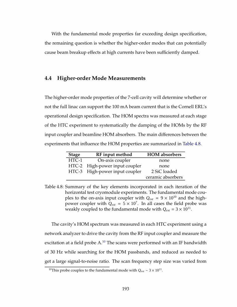
With the fundamental mode properties far exceeding design specification,
the remaining question is whether the higher-order modes that can potentially
cause beam breakup effects at high currents have been sufficiently damped.
4.4 Higher-order Mode Measurements
The higher-order mode properties of the 7-cell cavity will determine whether or
not the full linac can support the 100 mA beam current that is the Cornell ERL’s
operational design specification. The HOM spectra was measured at each stage
of the HTC experiment to systematically the damping of the HOMs by the RF
input coupler and beamline HOM absorbers. The main differences between the
experiments that influence the HOM properties are summarized in Table 4.8.
Stage RF input method HOM absorbers
HTC-1 On-axis coupler noneHTC-2 High-power input coupler noneHTC-3 High-power input coupler 2 SiC loaded
ceramic absorbers
Table 4.8: Summary of the key elements incorporated in each iteration of thehorizontal test cryomodule experiments. The fundamental mode cou-ples to the on-axis input coupler with Qext = 9 × 10¹⁰ and the high-power coupler with Qext = 5 × 10⁷. In all cases the field probe wasweakly coupled to the fundamental mode with Qext = 3× 10¹¹.
The cavity’s HOM spectrum was measured in each HTC experiment using a
network analyzer to drive the cavity from the RF input coupler and measure the
excitation at a field probe A.10 The scans were performed with an IF bandwidth
of 30 Hz while searching for the HOM passbands, and reduced as needed to
get a large signal-to-noise ratio. The scan frequency step size was varied from
10This probe couples to the fundamental mode with Qext ∼ 3× 10¹¹.
193
1 kHz/step for a broad scan to 1 Hz/point for modes with very large loaded
quality factors. The scattering parameter S 21 was measured as a function of
frequency and yields the properties of higher-order modes.
The most important figures of merit come from the HOM spectra of HTC-3,
since this will characterize the performance of the HOM absorbers, which are
not present in HTC-1 or HTC-2. Still, the spectra from the first two experiments
serve as a point of comparison to determine the efficiency of the absorbing ma-
terial in a realistic accelerator environment.
A final verification of HOM damping in HTC-3 is done with a beam to search
for any possible HOM having a large QL and (R/Q) which might have been
missed in network analyzer measurements.11
4.4.1 Methods to Extract Resonance Properties from Spectra
There are several methods to extract the properties of higher-order modes from
spectral measurements of the cavity’s scattering matrix. Two techniques were
implemented. The first fits the amplitude of S 21 with a Lorentzian function,
using the resonant frequency and quality factors as tuning parameters. The sec-
ond uses the complex phase information of S 21 to fit phase vs frequency near an
HOM, extracting the same information as in the Lorentzian case.12 The deriva-
tion of the equations is based on a circuit model of an HOM in the cavity.
A cavity containing a single HOM can be modeled as a transmission line
11This is possible if a HOM is trapped in the center of a cavity, having very weak coupling tothe probes used to measure a transfer function.
12While complex scattering parameter measurements could be used to fit the resonance curvedirectly, it is useful to use the amplitude formulation, since this technique is applicable whenusing spectrum analyzers, which lack phase information.
194

connected to an RLC circuit. [PA98] To determine the transfer function that will
be observed by the network analyzer, consider the simplified system of a volt-
age source varying sinusoidally at an angular frequency ω connected to a series
RLC circuit as shown in Figure 4.37.
Figure 4.37: HOM in cavity modelled as a series RLC circuit driven by a voltagesource, V , having sinusoidal time dependence.
The transfer function, measured across the resistor, of the RLC circuit driven
at an angular frequency ω is given by
H(ω) ≡ VR
V=
R
R + 1iωC + iωL
=
R
R + i(
ωL − 1ωC
), (4.4)
where VR is the voltage across the resistor.
Equation 4.4 can be written in terms of the squared amplitude and phase to
yield the following relations:
|H(ω)|2 =R2
R2 +(
ωL − 1ωC
)2, (4.5)
tan(φ) ≡ ℑ
H(ω)
ℜ
H(ω) =
ωL − 1ωC
R. (4.6)
Note that φ ≡ arg[H(ω)].
195
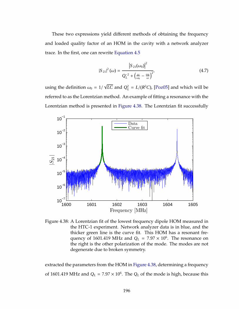
These two expressions yield different methods of obtaining the frequency
and loaded quality factor of an HOM in the cavity with a network analyzer
trace. In the first, one can rewrite Equation 4.5
|S 21|2 (ω) =
∣∣∣S 21(ω0)
∣∣∣2
Q−2L +
(ωω0− ω0
ω
)2, (4.7)
using the definition ω0 = 1/√
LC and Q2L = L/(R2C), [Poz05] and which will be
referred to as the Lorentzian method. An example of fitting a resonance with the
Lorentzian method is presented in Figure 4.38. The Lorentzian fit successfully
1600 1601 1602 1603 1604 160510
−7
10−6
10−5
10−4
10−3
10−2
10−1
|S21|
Frequency [MHz]
DataCurve fit
Figure 4.38: A Lorentzian fit of the lowest frequency dipole HOM measured inthe HTC-1 experiment. Network analyzer data is in blue, and thethicker green line is the curve fit. This HOM has a resonant fre-quency of 1601.419 MHz and QL = 7.97× 10⁶. The resonance onthe right is the other polarization of the mode. The modes are notdegenerate due to broken symmetry.
extracted the parameters from the HOM in Figure 4.38, determining a frequency
of 1601.419 MHz and QL = 7.97× 10⁶. The QL of the mode is high, because this
196
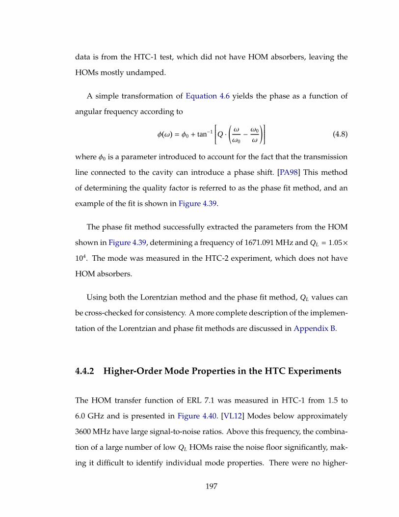
data is from the HTC-1 test, which did not have HOM absorbers, leaving the
HOMs mostly undamped.
A simple transformation of Equation 4.6 yields the phase as a function of
angular frequency according to
φ(ω) = φ0 + tan−1
Q ·(
ω
ω0− ω0
ω
)
(4.8)
where φ0 is a parameter introduced to account for the fact that the transmission
line connected to the cavity can introduce a phase shift. [PA98] This method
of determining the quality factor is referred to as the phase fit method, and an
example of the fit is shown in Figure 4.39.
The phase fit method successfully extracted the parameters from the HOM
shown in Figure 4.39, determining a frequency of 1671.091 MHz and QL = 1.05×
104. The mode was measured in the HTC-2 experiment, which does not have
HOM absorbers.
Using both the Lorentzian method and the phase fit method, QL values can
be cross-checked for consistency. A more complete description of the implemen-
tation of the Lorentzian and phase fit methods are discussed in Appendix B.
4.4.2 Higher-Order Mode Properties in the HTC Experiments
The HOM transfer function of ERL 7.1 was measured in HTC-1 from 1.5 to
6.0 GHz and is presented in Figure 4.40. [VL12] Modes below approximately
3600 MHz have large signal-to-noise ratios. Above this frequency, the combina-
tion of a large number of low QL HOMs raise the noise floor significantly, mak-
ing it difficult to identify individual mode properties. There were no higher-
197

1670.7 1670.8 1670.9 1671 1671.1 1671.2 1671.3 1671.4 1671.5−2
−1.5
−1
−0.5
0
0.5
1
1.5
2
Phase
[radia
n]
Frequency [MHz]
DataCurve fit
Figure 4.39: A phase fit of a HOM in the lowest dipole passband measured inthe HTC-2 experiment. Network analyzer data is in blue, and thered line is the curve fit. This HOM has a resonant frequency of1671.091 MHz and QL = 1.05× 10⁴.
order mode absorbers in HTC-1, so the QLs of the modes are much higher than
when HOM dampers are present in the HTC-3 experiment.
|S21|
Frequency [MHz]1500 2000 2500 3000 3500 4000 4500 5000 5500 6000
10−5
10−3
10−1
Figure 4.40: Network analyzer measurement of |S 21| from 1.5 to 6.0 GHz in HTC-1. The cavity’s temperature during the measurement was main-tained at 1.8 K. Spectra was taken using an axial probe as input andfield probe A as output.
Several features of the cavity can readily be determined from the spectra.
198
The first is the face that there are no monopole modes within 1.5 MHz of the
first two harmonics of 2.6 GHz.13 This is important, because a high QL monopole
mode at a harmonic of the bunch frequency would result in resonant excitation
of this mode and overload the HOM absorbers. [BBB+11]
In the spectra, it is possible to readily identify various dipole, quadrupole,
sextupole and octupole modes. The first instance of passbands containing these
modes (along with other modes with similar frequencies) is presented in Fig-
ure 4.41. The dipole modes are recognizable as two modes very close in fre-
quency with similar HOM properties. While in a cylindrically symmetric struc-
ture their frequencies would be identical, symmetry breaking features such as
the side coupler port introduces small perturbations that lead to frequency split-
ting. Similarly quadrupole, sextupole and octupole modes can be identified by
4, 6 or 8 resonances near a central frequency, though symmetry makes some of
these modes degenerate.
Because HTC-1 uses an axial field probe to drive the cavity, the structure is
close to azimuthally symmetric and modes can be computed with a 2.5D elec-
tromagnetic code such as CLANS. The modes were simulated up to 3.6 GHz–the
frequency at which the signal to noise ratio was large enough to extract HOM
properties–and compared with experimental measurements. The comparison
between modes in HTC-1 and the CLANS results are shown in Figure 4.42.
Measurements of the HOM spectra are found to agree in frequency, but show
some discrepancy in quality factor. The first few quadrupole, sextupole and
octupole passbands have modes with frequency below the cutoff frequency of
the beam tubes, resulting in small coupling to the HOM loads. This will not
13The ERL operates at 1.3 GHz with bunches spaced by 180, making the repetition rate2.6 GHz.
199
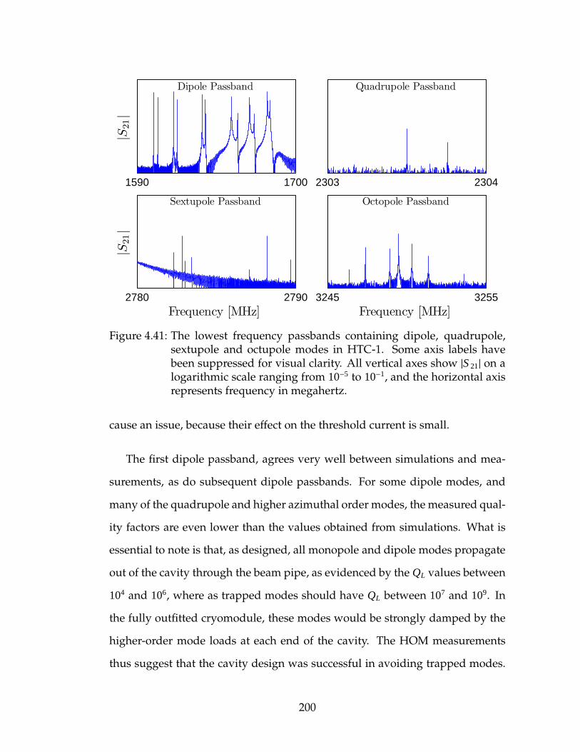
1590 1700
Dipole Passband
|S21|
2303 2304
Quadrupole Passband
2780 2790
Sextupole Passband
Frequency [MHz]
|S21|
3245 3255
Octopole Passband
Frequency [MHz]
Figure 4.41: The lowest frequency passbands containing dipole, quadrupole,sextupole and octupole modes in HTC-1. Some axis labels havebeen suppressed for visual clarity. All vertical axes show |S 21| on alogarithmic scale ranging from 10−5 to 10−1, and the horizontal axisrepresents frequency in megahertz.
cause an issue, because their effect on the threshold current is small.
The first dipole passband, agrees very well between simulations and mea-
surements, as do subsequent dipole passbands. For some dipole modes, and
many of the quadrupole and higher azimuthal order modes, the measured qual-
ity factors are even lower than the values obtained from simulations. What is
essential to note is that, as designed, all monopole and dipole modes propagate
out of the cavity through the beam pipe, as evidenced by the QL values between
104 and 106, where as trapped modes should have QL between 107 and 109. In
the fully outfitted cryomodule, these modes would be strongly damped by the
higher-order mode loads at each end of the cavity. The HOM measurements
thus suggest that the cavity design was successful in avoiding trapped modes.
200
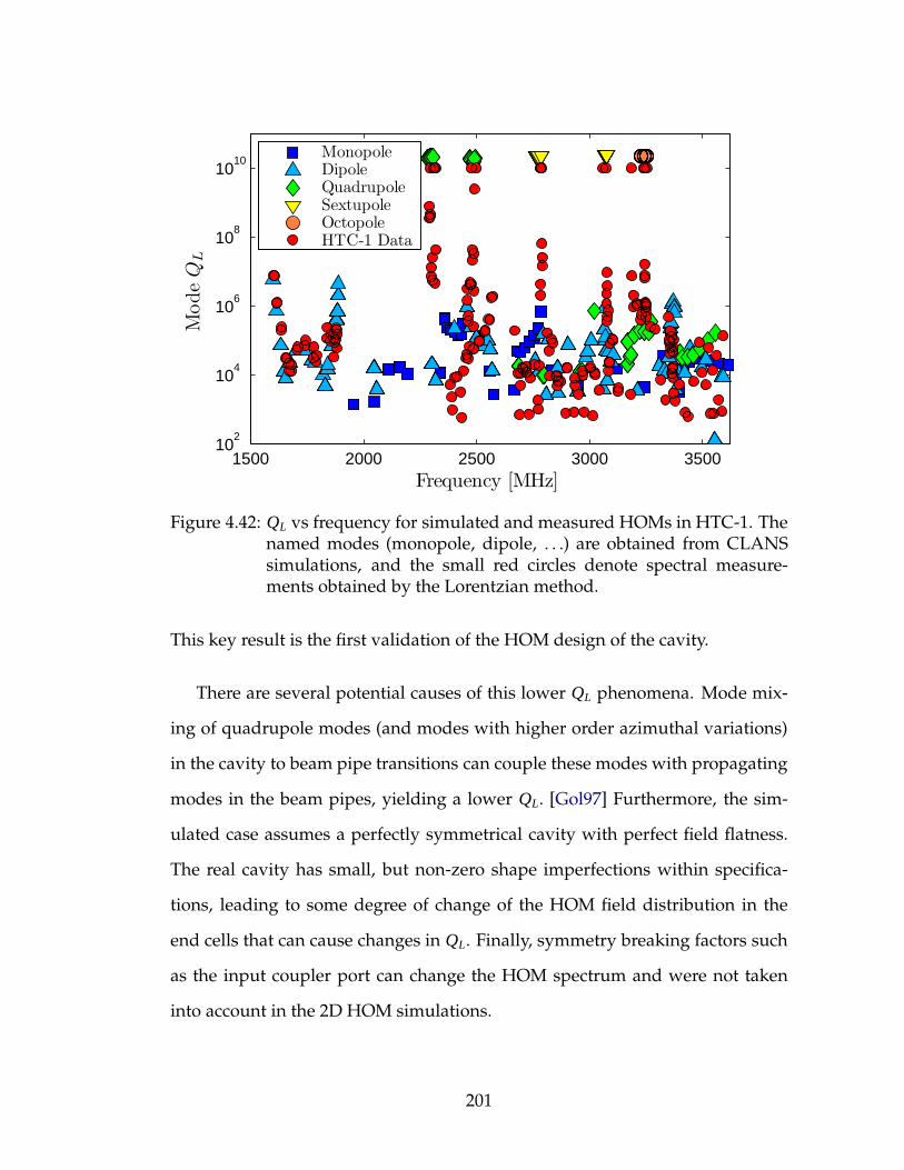
1500 2000 2500 3000 350010
2
104
106
108
1010
Frequency [MHz]
Mode
QL
MonopoleDipoleQuadrupoleSextupoleOctopoleHTC-1 Data
Figure 4.42: QL vs frequency for simulated and measured HOMs in HTC-1. Thenamed modes (monopole, dipole, . . .) are obtained from CLANSsimulations, and the small red circles denote spectral measure-ments obtained by the Lorentzian method.
This key result is the first validation of the HOM design of the cavity.
There are several potential causes of this lower QL phenomena. Mode mix-
ing of quadrupole modes (and modes with higher order azimuthal variations)
in the cavity to beam pipe transitions can couple these modes with propagating
modes in the beam pipes, yielding a lower QL. [Gol97] Furthermore, the sim-
ulated case assumes a perfectly symmetrical cavity with perfect field flatness.
The real cavity has small, but non-zero shape imperfections within specifica-
tions, leading to some degree of change of the HOM field distribution in the
end cells that can cause changes in QL. Finally, symmetry breaking factors such
as the input coupler port can change the HOM spectrum and were not taken
into account in the 2D HOM simulations.
201
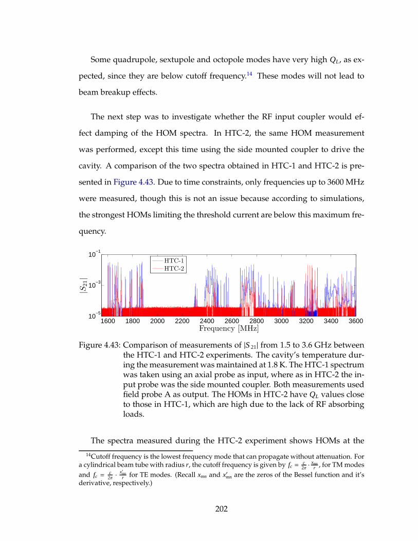
Some quadrupole, sextupole and octopole modes have very high QL, as ex-
pected, since they are below cutoff frequency.14 These modes will not lead to
beam breakup effects.
The next step was to investigate whether the RF input coupler would ef-
fect damping of the HOM spectra. In HTC-2, the same HOM measurement
was performed, except this time using the side mounted coupler to drive the
cavity. A comparison of the two spectra obtained in HTC-1 and HTC-2 is pre-
sented in Figure 4.43. Due to time constraints, only frequencies up to 3600 MHz
were measured, though this is not an issue because according to simulations,
the strongest HOMs limiting the threshold current are below this maximum fre-
quency.
|S21|
Frequency [MHz]
1600 1800 2000 2200 2400 2600 2800 3000 3200 3400 360010
−5
10−3
10−1
HTC-1HTC-2
Figure 4.43: Comparison of measurements of |S 21| from 1.5 to 3.6 GHz betweenthe HTC-1 and HTC-2 experiments. The cavity’s temperature dur-ing the measurement was maintained at 1.8 K. The HTC-1 spectrumwas taken using an axial probe as input, where as in HTC-2 the in-put probe was the side mounted coupler. Both measurements usedfield probe A as output. The HOMs in HTC-2 have QL values closeto those in HTC-1, which are high due to the lack of RF absorbingloads.
The spectra measured during the HTC-2 experiment shows HOMs at the
14Cutoff frequency is the lowest frequency mode that can propagate without attenuation. Fora cylindrical beam tube with radius r, the cutoff frequency is given by fc = c
2π ·xmnr , for TM modes
and fc = c2π ·
x′mnr for TE modes. (Recall xmn and x′mn are the zeros of the Bessel function and it’s
derivative, respectively.)
202
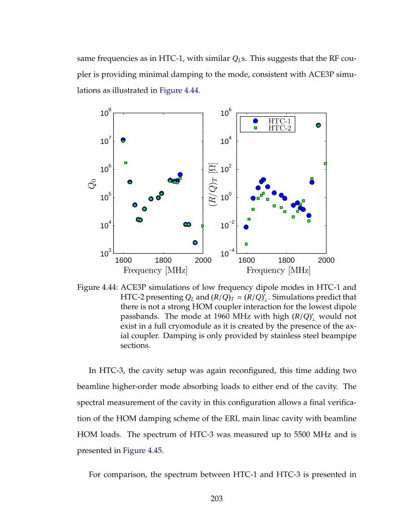
same frequencies as in HTC-1, with similar QLs. This suggests that the RF cou-
pler is providing minimal damping to the mode, consistent with ACE3P simu-
lations as illustrated in Figure 4.44.
1600 1800 200010
3
104
105
106
107
108
Q0
Frequency [MHz]1600 1800 2000
10−4
10−2
100
102
104
106
(R/Q
) T[Ω
]
Frequency [MHz]
HTC-1HTC-2
Figure 4.44: ACE3P simulations of low frequency dipole modes in HTC-1 andHTC-2 presenting QL and (R/Q)T = (R/Q)′⊥. Simulations predict thatthere is not a strong HOM coupler interaction for the lowest dipolepassbands. The mode at 1960 MHz with high (R/Q)′⊥ would notexist in a full cryomodule as it is created by the presence of the ax-ial coupler. Damping is only provided by stainless steel beampipesections.
In HTC-3, the cavity setup was again reconfigured, this time adding two
beamline higher-order mode absorbing loads to either end of the cavity. The
spectral measurement of the cavity in this configuration allows a final verifica-
tion of the HOM damping scheme of the ERL main linac cavity with beamline
HOM loads. The spectrum of HTC-3 was measured up to 5500 MHz and is
presented in Figure 4.45.
For comparison, the spectrum between HTC-1 and HTC-3 is presented in
203

|S21|
Frequency [MHz]2000 2500 3000 3500 4000 4500 5000 5500
10−6
10−5
10−4
Figure 4.45: Measurement of |S 21| from 1.5 to 5.5 GHz of ERL 7.1 in HTC-3. Thecavity’s temperature during the measurement was maintained at1.8 K. Spectra was taken using the side mounted RF coupler asinput and field probe A as output. The transmitted signal levelis much lower than in HTC-1 or HTC-2 measurements due to thepresence of strongly damping RF absorbing loads.
Figure 4.46. The noise floor below 3600 MHz is reduced by more than an or-
der of magnitude between the HTC-1 and HTC-3 measurements, which can be
attributed to the RF absorbers. There are also significantly fewer modes that
are able to be measured, due to the strong damping, showing that the beamline
absorbers efficiently provide broadband damping of HOMs.
|S21|
Frequency [MHz]
2000 2500 3000 3500 4000 4500 5000 550010
−6
10−4
10−2 HTC-1
HTC-3
Figure 4.46: Comparison of |S 21| spectra between HTC-1 and HTC-3 from 1.5to 5.5 GHz. The cavity’s temperature during the measurementwas maintained at 1.8 K. The lack of very high QL resonances inthe HTC-3 measurement demonstrates the efficacy of the beamlineHOM absorbing scheme.
Figure 4.47, Table 4.9, and Table 4.10 present the properties of HOM modes
measured in HTC-3. The frequencies agree with simulations, but loaded qual-
204
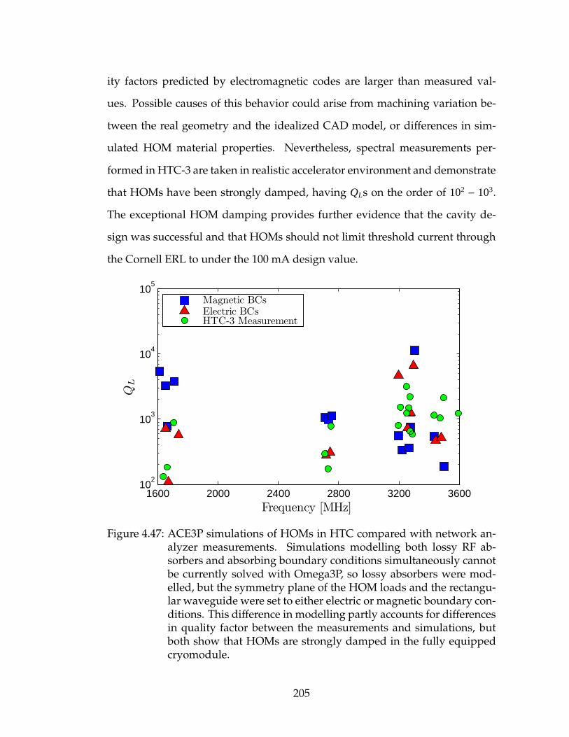
ity factors predicted by electromagnetic codes are larger than measured val-
ues. Possible causes of this behavior could arise from machining variation be-
tween the real geometry and the idealized CAD model, or differences in sim-
ulated HOM material properties. Nevertheless, spectral measurements per-
formed in HTC-3 are taken in realistic accelerator environment and demonstrate
that HOMs have been strongly damped, having QLs on the order of 102 − 103.
The exceptional HOM damping provides further evidence that the cavity de-
sign was successful and that HOMs should not limit threshold current through
the Cornell ERL to under the 100 mA design value.
1600 2000 2400 2800 3200 360010
2
103
104
105
Frequency [MHz]
QL
Magnetic BCsElectric BCsHTC-3 Measurement
Figure 4.47: ACE3P simulations of HOMs in HTC compared with network an-alyzer measurements. Simulations modelling both lossy RF ab-sorbers and absorbing boundary conditions simultaneously cannotbe currently solved with Omega3P, so lossy absorbers were mod-elled, but the symmetry plane of the HOM loads and the rectangu-lar waveguide were set to either electric or magnetic boundary con-ditions. This difference in modelling partly accounts for differencesin quality factor between the measurements and simulations, butboth show that HOMs are strongly damped in the fully equippedcryomodule.
205

f0 [MHz] QL f0 [MHz] QL f0 [MHz] QL f0 [MHz] QL
1637.4117 1.32e2 3630.3944 1.04e6 3809.0307 1.90e3 4039.1344 2.68e31662.6128 1.83e2 3630.9727 5.27e5 3813.9569 1.97e5 4047.5938 9.40e21705.3440 8.86e2 3636.4594 1.56e6 3816.1146 3.16e3 4061.6825 1.68e32708.4012 2.95e2 3640.0009 2.87e2 3819.9457 1.16e5 4074.0674 1.01e32728.9106 1.73e2 3642.0975 9.67e4 3825.6921 1.12e5 4079.8158 2.59e32748.6406 7.84e2 3643.6910 7.14e4 3831.8272 1.34e3 4081.3894 2.03e33194.9459 8.05e2 3647.0764 1.59e5 3832.1174 9.24e5 4084.5994 1.46e33210.6628 1.53e3 3647.9088 1.13e5 3838.7176 2.57e3 4088.8181 1.46e33248.9539 3.18e3 3647.9211 6.27e4 3841.9901 3.93e3 4094.0225 1.13e33251.6725 1.24e3 3652.5325 3.30e4 3843.0820 2.29e3 4104.3871 2.40e33264.5710 1.49e3 3660.8575 4.76e3 3848.9038 2.00e3 4120.6256 1.05e33272.2906 2.20e3 3671.0948 2.04e3 3890.8351 5.15e3 4123.7216 7.03e23274.7617 6.51e2 3723.3290 8.51e2 3897.6500 6.52e2 4137.6914 1.04e33288.4388 5.89e2 3738.0247 6.98e2 3910.0731 1.49e3 4140.3136 5.22e33431.7733 1.15e3 3745.0022 6.33e2 3940.6970 1.42e3 4146.3533 2.73e33473.2295 1.04e3 3758.9201 4.26e3 3946.5141 2.62e3 4149.4583 3.46e43495.4240 2.12e3 3765.6838 3.76e2 3953.5589 5.80e2 4152.3073 3.34e43592.1809 1.23e3 3775.2054 4.62e3 3975.1453 1.72e3 4156.2950 1.13e43617.9073 9.90e5 3780.5399 1.87e3 4009.5183 9.06e2 4161.5823 1.30e33618.7104 1.46e3 3801.0156 1.49e3 4014.5007 5.66e3 4169.9621 3.32e33620.8522 1.80e5 3806.3779 7.78e4 4027.1821 5.06e3 4209.7840 2.32e53623.8689 1.17e6 3806.6699 1.48e5 4033.9365 7.10e3 4211.9027 5.09e3
Table 4.9: List of higher-order mode properties measured in HTC-3 (1 of 2).
4.5 HTC Testing with Beam
The HTC was installed in the Cornell ERL injector cryomodule beam line, and
initial tests of the structure with high current electron beam began in Fall 2013.
The objective of the experiment is to obtain a beam based measurement of HOM
properties, by exciting HOMs in the cavity with an off-axis beam. [VBLM12]
Following the methodology discussed in [Far98] and [Bab01], for a bunch
repetition frequency, fb, a HOM resonating at fλ is excited by modulating the
bunch charge of the beam such that
qn = q0
[
1+ amodsin(
2πn fmod/ fb + φmod)]
. (4.9)
206
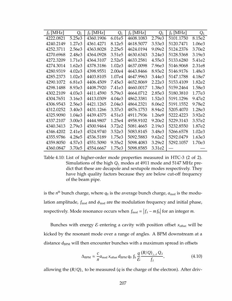
f0 [MHz] QL f0 [MHz] QL f0 [MHz] QL f0 [MHz] QL
4222.0821 5.25e3 4360.1906 6.01e5 4608.1083 2.79e3 5101.1750 8.15e24240.2149 1.27e3 4361.4271 8.12e5 4618.5077 3.53e3 5120.7471 1.06e34252.3711 2.56e3 4363.8028 2.25e5 4624.0194 9.09e2 5124.2376 3.70e24270.6968 2.48e3 4364.0928 3.51e5 4630.6343 3.24e3 5128.5368 3.19e34272.3209 1.71e3 4364.3107 2.52e5 4633.2581 4.55e3 5133.6280 5.41e24274.3014 1.62e3 4378.3186 1.02e3 4637.0098 7.96e3 5146.9068 2.31e84280.9319 4.02e3 4398.9551 2.00e4 4643.8466 8.93e2 5146.9176 1.48e34285.2373 1.02e3 4403.8105 1.07e4 4647.9963 3.44e3 5147.1788 4.18e74290.1072 6.81e3 4406.4509 7.45e3 4652.8069 2.22e3 5153.4109 1.82e24298.1488 8.93e3 4408.7920 7.41e3 4660.0017 1.38e3 5159.2464 1.58e34302.2109 4.03e3 4411.4590 5.79e3 4664.0712 2.85e3 5180.3810 1.77e34304.7651 3.16e3 4413.0309 4.04e3 4862.3381 1.52e3 5191.1296 9.47e24306.9543 2.56e3 4421.1265 2.04e3 4864.2321 8.06e2 5191.1552 9.78e24312.0252 3.40e3 4431.1266 3.37e3 4876.1753 8.94e2 5205.4070 1.28e34325.9090 1.04e3 4439.4375 4.51e3 4911.7936 1.26e9 5222.4223 3.92e24337.2107 3.00e3 4444.9807 1.25e4 4958.9102 9.20e2 5229.3143 3.57e24340.3413 2.79e3 4500.9464 3.72e2 5081.4665 2.19e3 5232.8550 1.87e24346.4202 2.41e3 4524.9740 3.52e3 5083.8145 3.48e3 5266.6578 1.02e34355.9786 4.28e5 4536.5189 1.75e3 5092.5883 9.62e2 5292.0479 1.63e34359.8050 4.57e3 4551.5090 9.35e2 5098.4083 3.29e2 5292.1057 1.70e34360.0847 3.70e5 4554.6667 1.75e3 5098.8585 3.31e2 — —
Table 4.10: List of higher-order mode properties measured in HTC-3 (2 of 2).Simulations of the high QL modes at 4911 mode and 5147 MHz pre-dict that these are decapole and sextupole modes respectively. Theyhave high quality factors because they are below cut-off frequencyof the beam pipe.
is the nth bunch charge, where q0 is the average bunch charge, amod is the modu-
lation amplitude, fmod and φmod are the modulation frequency and initial phase,
respectively. Mode resonance occurs when fmod =∣∣∣ fλ − m fb
∣∣∣ for an integer m.
Bunches with energy E entering a cavity with position offset xoffset will be
kicked by the resonant mode over a range of angles. A BPM downstream at a
distance dBPM will then encounter bunches with a maximum spread in offsets
∆BPM ≈cπ
amod xoffsetdBPM q0 fbqE
(
R/Q)
⊥,λ Qλ
fλ, (4.10)
allowing the (R/Q)⊥ to be measured (q is the charge of the electron). After driv-
207
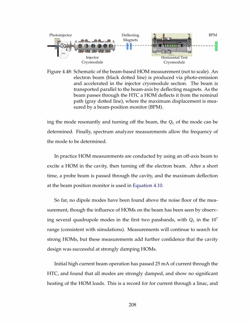
Figure 4.48: Schematic of the beam-based HOM measurement (not to scale). Anelectron beam (black dotted line) is produced via photo-emissionand accelerated in the injector cryomodule section. The beam istransported parallel to the beam-axis by deflecting magnets. As thebeam passes through the HTC a HOM deflects it from the nominalpath (gray dotted line), where the maximum displacement is mea-sured by a beam-position monitor (BPM).
ing the mode resonantly and turning off the beam, the QL of the mode can be
determined. Finally, spectrum analyzer measurements allow the frequency of
the mode to be determined.
In practice HOM measurements are conducted by using an off-axis beam to
excite a HOM in the cavity, then turning off the electron beam. After a short
time, a probe beam is passed through the cavity, and the maximum deflection
at the beam position monitor is used in Equation 4.10.
So far, no dipole modes have been found above the noise floor of the mea-
surement, though the influence of HOMs on the beam has been seen by observ-
ing several quadrupole modes in the first two passbands, with QL in the 107
range (consistent with simulations). Measurements will continue to search for
strong HOMs, but these measurements add further confidence that the cavity
design was successful at strongly damping HOMs.
Initial high current beam operation has passed 25 mA of current through the
HTC, and found that all modes are strongly damped, and show no significant
heating of the HOM loads. This is a record for for current through a linac, and
208

supplies further confidence that the cavity design and fabrication was success-
ful.
4.6 Mechanical Considerations
Mechanical vibrations can couple to electromagnetic fields, a phenomena
known as microphonics, which was first observed in work with normal con-
ducting resonators. [KSS67] As discussed in subsection 3.3.1, the coupler kick
to a beam is strongly dependent on the detuning of the cavity from microphon-
ics. Power requirements increase to maintain a constant cavity voltage when
liquid helium bath pressure fluctuations and other vibration sources change the
resonant frequency of the cavity (see Figure 4.49). [PL12c] For these reasons it
is important to characterize the level of microphonics present in the cavity and
ensure they are within the Cornell ERL design specification of ±20 Hz peak de-
tuning.
Measurements of the microphonics levels for ERL 7.1 installed in the HTC
is presented in Figure 4.50, demonstrate that peak detuning is within the de-
sign specifications. [PL12a] In addition, both the slow frequency tuner and fast
piezo-electric tuner were tested and found to operate with very low hysteresis,
which is important for cavity frequency control. [PL12a] Studies of Lorentz force
detuning of the cavity and sensitivity to pressure fluctuations found agreement
between simulations and measurement. [PL12b] All mechanical systems func-
tioned properly and within specification, validating the cryomodule design.
209
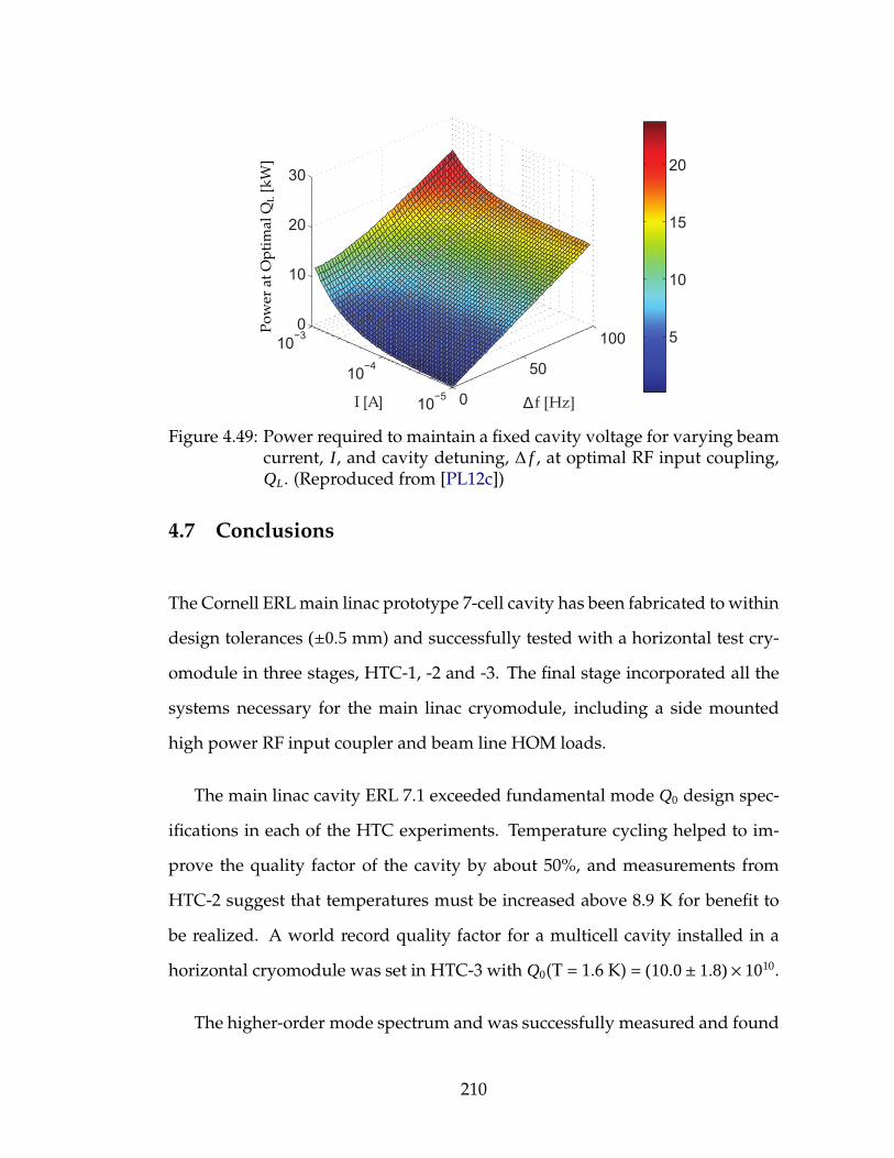
Figure 4.49: Power required to maintain a fixed cavity voltage for varying beamcurrent, I, and cavity detuning, ∆ f , at optimal RF input coupling,QL. (Reproduced from [PL12c])
4.7 Conclusions
The Cornell ERL main linac prototype 7-cell cavity has been fabricated to within
design tolerances (±0.5 mm) and successfully tested with a horizontal test cry-
omodule in three stages, HTC-1, -2 and -3. The final stage incorporated all the
systems necessary for the main linac cryomodule, including a side mounted
high power RF input coupler and beam line HOM loads.
The main linac cavity ERL 7.1 exceeded fundamental mode Q0 design spec-
ifications in each of the HTC experiments. Temperature cycling helped to im-
prove the quality factor of the cavity by about 50%, and measurements from
HTC-2 suggest that temperatures must be increased above 8.9 K for benefit to
be realized. A world record quality factor for a multicell cavity installed in a
horizontal cryomodule was set in HTC-3 with Q0(T = 1.6 K) = (10.0± 1.8)× 1010.
The higher-order mode spectrum and was successfully measured and found
210
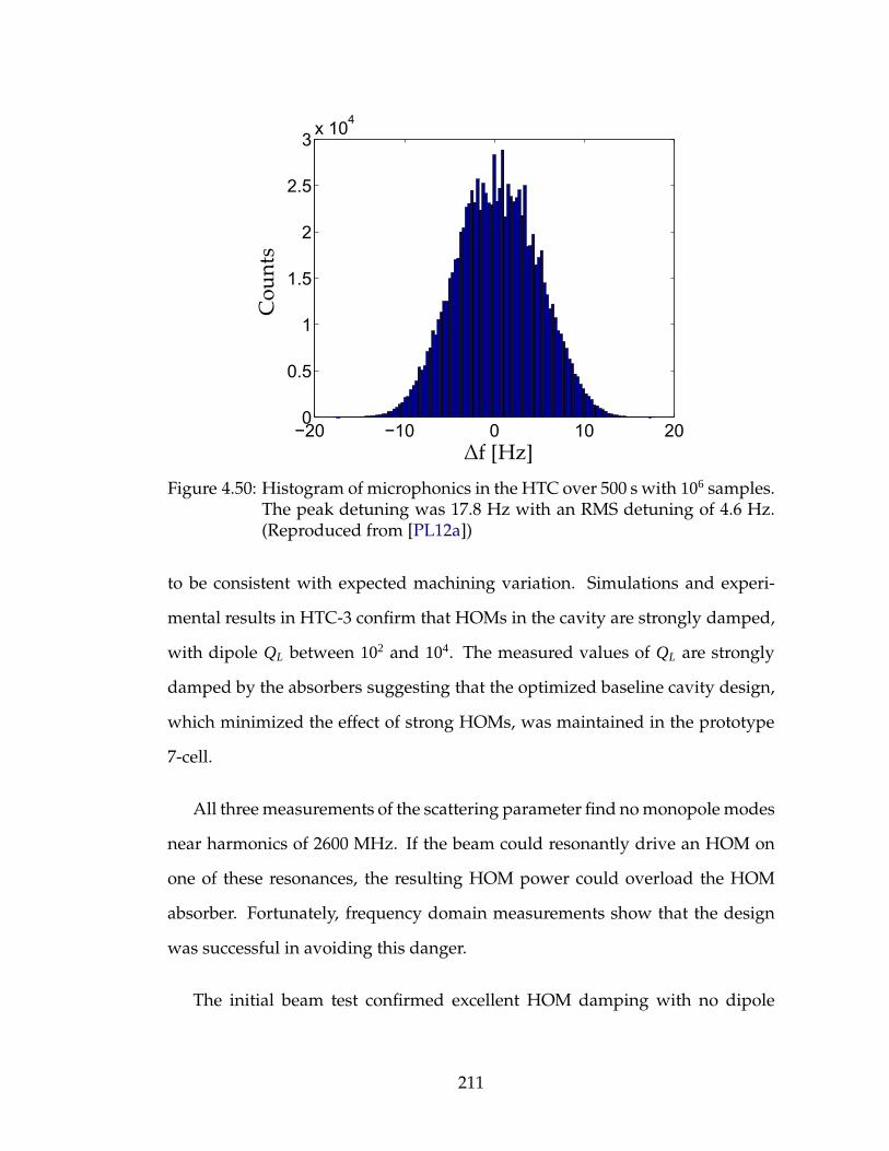
Figure 4.50: Histogram of microphonics in the HTC over 500 s with 106 samples.The peak detuning was 17.8 Hz with an RMS detuning of 4.6 Hz.(Reproduced from [PL12a])
to be consistent with expected machining variation. Simulations and experi-
mental results in HTC-3 confirm that HOMs in the cavity are strongly damped,
with dipole QL between 102 and 104. The measured values of QL are strongly
damped by the absorbers suggesting that the optimized baseline cavity design,
which minimized the effect of strong HOMs, was maintained in the prototype
7-cell.
All three measurements of the scattering parameter find no monopole modes
near harmonics of 2600 MHz. If the beam could resonantly drive an HOM on
one of these resonances, the resulting HOM power could overload the HOM
absorber. Fortunately, frequency domain measurements show that the design
was successful in avoiding this danger.
The initial beam test confirmed excellent HOM damping with no dipole
211

mode having a high (R/Q) · Q found as of this writing. In addition, the cav-
ity supports beam current in excess of 25 mA, a record in a CW linac.
In conclusion, the prototype 7-cell cavity ERL 7.1 was shown to exceed all
design specifications and should deliver excellent performance as the driver for
the main linac of Cornell’s Energy Recovery Linac.
212
CHAPTER 5
FINAL SUMMARY
This thesis has presented research pushing back three frontiers of SRF sci-
ence: Gradient, CW beam power, and Quality Factor.
On the first frontier, this thesis demonstrates that the superheating field fun-
damentally limits the maximal surface magnetic field on superconducting nio-
bium structures, not the lower critical field, Bc1, as has sometimes been sug-
gested. For typical surface preparation of niobium cavities used in large scale
accelerators, (electropolish, or buffer chemical polish, followed by a 120C heat
treatment), surface magnetic fields of 200 mT at 0 K is the ultimate limit set
by the superheating field, though this may be improved slightly via mate-
rial treatment making the surface layer nearly type-I. Already, there are hints
that this ultimate surface field limit is being reached in accelerating struc-
tures. [KCG+12, RAG+11] Theoretical and experimental results agree: niobium
is reaching its highest sustainable gradients.
To make further progress on this frontier, new materials should be devel-
oped as a replacement for niobium. Theoretical work has demonstrated that
the use of Nb3Sn in superconducting accelerating structures could double the
maximum gradient. [CS08, Pos13b] To this end, Cornell has a research and de-
velopment program ongoing to fabricate Nb3Sn structures and initial results are
encouraging, demonstrating surface fields in excess of Bc1. [Pos13a] With contin-
ued research and development of Nb3Sn, a new generation of higher gradient
machines is on the horizon.
Progress has also been made on the CW beam power frontier. Prior to this
213

work, the maximal measured current in an ERL was 9 mA, before being lim-
ited by beam breakup effects. [Ten06] Initial simulations suggested that beam
breakup due to trapped dipole modes could occur at currents much less than
the 100 mA specification needed for the Cornell ERL. Work presented in this
thesis on designing an optimized, robust cavity with strongly damped higher-
order modes has shown that an ERL consisting of realistic cavities can support
threshold current of over 300 mA. The findings of this thesis demonstrate that
an improvement factor of 30 in beam breakup current is achievable in SRF CW
linacs.
Advances have also been made in intrinsic cavity quality factor, the final
frontier. The proposed design specification for the Cornell ERL main linac cavi-
ties of reaching Q0 = 2×10¹⁰ at 1.8 K and 16.2 MV/m has been more than tripled,
obtaining Q0 above 6× 10¹⁰ at the same operating gradient and temperature in
a fully outfitted cryomodule. Moreover, a multi-cell cryomodule world record
has been set for niobium cavities, reaching values in excess of 1× 10¹¹. Routine
production of cavities reproducing this result would allow for operation of the
ERL at 1.6 K with substantial energy savings.
In closing, SRF science has demonstrated the capacity to produce workhorse
CW linear particle accelerators able to push to higher average beam currents,
and with higher efficiently than any other accelerating technology. The hope is
that this thesis has helped to make the future of SRF just a little brighter.
214
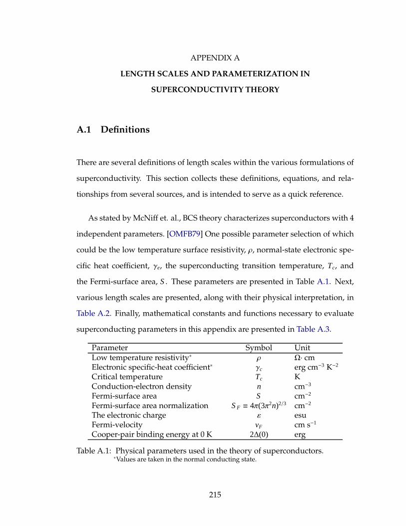
APPENDIX A
LENGTH SCALES AND PARAMETERIZATION IN
SUPERCONDUCTIVITY THEORY
A.1 Definitions
There are several definitions of length scales within the various formulations of
superconductivity. This section collects these definitions, equations, and rela-
tionships from several sources, and is intended to serve as a quick reference.
As stated by McNiff et. al., BCS theory characterizes superconductors with 4
independent parameters. [OMFB79] One possible parameter selection of which
could be the low temperature surface resistivity, ρ, normal-state electronic spe-
cific heat coefficient, γe, the superconducting transition temperature, Tc, and
the Fermi-surface area, S . These parameters are presented in Table A.1. Next,
various length scales are presented, along with their physical interpretation, in
Table A.2. Finally, mathematical constants and functions necessary to evaluate
superconducting parameters in this appendix are presented in Table A.3.
Parameter Symbol UnitLow temperature resistivity∗ ρ Ω· cmElectronic specific-heat coefficient∗ γc erg cm−3 K−2
Critical temperature Tc KConduction-electron density n cm−3
Fermi-surface area S cm−2
Fermi-surface area normalization S F ≡ 4π(3π2n)2/3 cm−2
The electronic charge ε esuFermi-velocity vF cm s−1
Cooper-pair binding energy at 0 K 2∆(0) erg
Table A.1: Physical parameters used in the theory of superconductors.∗Values are taken in the normal conducting state.
215

Symbol Interpretation Equationℓtr Normal-conducting electronic mean free
path. Characterizes the ”cleanliness” (ℓtr →∞) or ”dirtiness” (ℓtr → 0) of a supercon-ductor. [MS69]
Eq. A.1 [OMFB79]
ξ0 BCS coherence length of a clean supercon-ductor. Rough spatial extent of Cooperpairs. [Son98]
Eq. A.3 [OMFB79]
ξGL Coherence length used in Ginzburg-Landau theory. The length scale overwhich the superconducting order param-eter fluxuates. Roughly the radius of oneflux quantum near the upper critical fieldof a Type-II superconductor. [Kit86]
Eq. A.13 [Kit86]
ξS Coherence length used in SRIMP. [Hal70b] Eq. A.19 [Hal70b]λL London penetration depth, measuring de-
cay constant of magnetic field within thebulk of a clean superconductor. [Kit86]
Eq. A.6 [OMFB79]
λGL Ginzburg-Landau penetration depth, char-acterizing the extent of order parame-ter penetration into superconducting bulk.[Kit86]
Eq. A.15 [OMFB79]
Table A.2: Characteristic length scales in the theory of superconductivity.
Parameter Symbol Definition Value
Euler’s number e∞∑
n=0
1n!
2.718
Euler-Mascheroni Constant γ limn→∞
n∑
k=1
1k− ln(n)
0.577
— eγ — 1.781
Zeta-function ζ(s)∞∑
n=1
1ns
—
— ζ(3) — 1.202
Gamma function Γ(z)∫ ∞
0tz−1e−t dt —
Digamma function ψ(z)ddz
lnΓ(z) —
Table A.3: Numerical functions and constants used in this appendix. Values aretruncated at three decimal places.
216
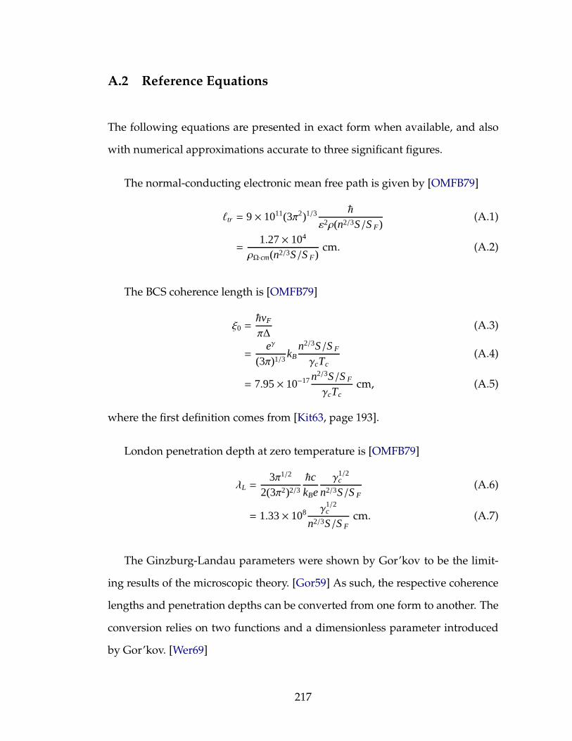
A.2 Reference Equations
The following equations are presented in exact form when available, and also
with numerical approximations accurate to three significant figures.
The normal-conducting electronic mean free path is given by [OMFB79]
ℓtr = 9× 10¹¹(3π2)1/3 ~
ε2ρ(n2/3S/S F)(A.1)
=1.27× 10⁴
ρΩ·cm(n2/3S/S F)cm. (A.2)
The BCS coherence length is [OMFB79]
ξ0 =~vF
π∆(A.3)
=eγ
(3π)1/3kB
n2/3S/S F
γcTc(A.4)
= 7.95× 10⁻¹⁷n2/3S/S F
γcTccm, (A.5)
where the first definition comes from [Kit63, page 193].
London penetration depth at zero temperature is [OMFB79]
λL =3π1/2
2(3π2)2/3
~ckBe
γ1/2c
n2/3S/S F(A.6)
= 1.33× 10⁸ γ1/2c
n2/3S/S Fcm. (A.7)
The Ginzburg-Landau parameters were shown by Gor’kov to be the limit-
ing results of the microscopic theory. [Gor59] As such, the respective coherence
lengths and penetration depths can be converted from one form to another. The
conversion relies on two functions and a dimensionless parameter introduced
by Gor’kov. [Wer69]
217

The Gor’kov χ function is written in terms of a sum, that can be solved in
terms of the digamma function and the zeta function:
χ(z) =
∑∞v=0(2v + 1)−2(2v + 1+ z)−1
∑∞v=0(2v + 1)−3
, (A.8)
=
π2z − 4(
γ + ln(4)+ ψ[
1+z2
])
7ζ(3)z2(A.9)
which is used later in the form of a helper function, R(z) defined as
R(z) = (1+ z)χ(z), (A.10)
and is plotted in Figure A.1.
10−1
100
101
102
103
104
1
1.04
1.08
1.12
1.16
1.2
λtr
R(λ
tr)
Figure A.1: Plot of R(λtr) vs λtr, showing that R is a slowly varying function thatis approximately unity. This function has limiting values R(0) = 1and R(∞) = π2/(7ζ(3)) ≈ 1.173. [Wer69]
These functions use a normalized length parameter λtr as an argument:
λtr =πe−γ
2· ξ0
ℓtr(A.11)
≈ 0.882ξ0
ℓtr. (A.12)
218
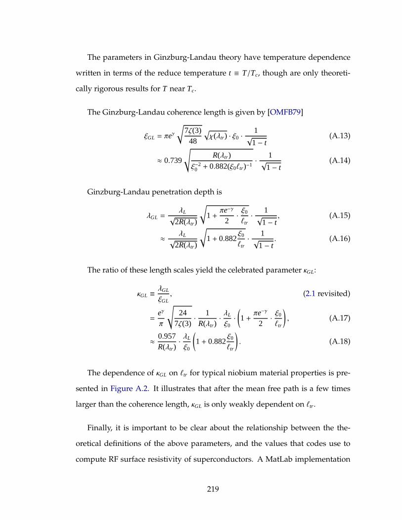
The parameters in Ginzburg-Landau theory have temperature dependence
written in terms of the reduce temperature t ≡ T/Tc, though are only theoreti-
cally rigorous results for T near Tc.
The Ginzburg-Landau coherence length is given by [OMFB79]
ξGL = πeγ√
7ζ(3)48
√
χ(λtr) · ξ0 ·1√1− t
(A.13)
≈ 0.739
√
R(λtr)
ξ−20 + 0.882(ξ0ℓtr)−1
· 1√1− t
(A.14)
Ginzburg-Landau penetration depth is
λGL =λL√
2R(λtr)
√
1+πe−γ
2· ξ0
ℓtr· 1√
1− t, (A.15)
≈ λL√2R(λtr)
√
1+ 0.882ξ0
ℓtr· 1√
1− t. (A.16)
The ratio of these length scales yield the celebrated parameter κGL:
κGL ≡λGL
ξGL, (2.1 revisited)
=eγ
π
√
247ζ(3)
· 1R(λtr)
· λL
ξ0·(
1+πe−γ
2· ξ0
ℓtr
)
, (A.17)
≈ 0.957R(λtr)
· λL
ξ0
(
1+ 0.882ξ0
ℓtr
)
. (A.18)
The dependence of κGL on ℓtr for typical niobium material properties is pre-
sented in Figure A.2. It illustrates that after the mean free path is a few times
larger than the coherence length, κGL is only weakly dependent on ℓtr.
Finally, it is important to be clear about the relationship between the the-
oretical definitions of the above parameters, and the values that codes use to
compute RF surface resistivity of superconductors. A MatLab implementation
219

10−1
100
101
102
103
100
101
102
103
ℓtr [nm]
κG
L
Typical NiobiumTypical Nb3Sn
Figure A.2: κGL vs ℓtr for typical niobium and Nb3Sn material properties.
of SRIMP [Hal70b] is used to carry out resistivity calculations in the work pre-
sented here, taking into account frequency, critical temperature, electronic mean
free path, normalized energy gap, London penetration depth, and coherence
length. All parameters listed are equivalent to the quantities named above with
two exceptions:
SRIMP defines the coherence length to be given by [Hal70b]
ξS =~vF
2∆(0)=π
2ξ0, (A.19)
and instead of normalizing the Cooper-pair energy gap in the standard method,
i.e. Eg = 2∆(0)/(kBTc), SRIMP expects an energy gap, ES , given by
ES =∆(0)kBTc
. (A.20)
For comparison, the literature lists the normalized energy gap, Eg, of Nio-
bium as 3.84, [MB57] and 3.6. [Per66, BGK59] SRIMP calculations for these ma-
220

terials would use ES = 1.92 and 1.8 respectively. SRIMP is discussed in Ap-
pendix C.
221
APPENDIX B
HIGHER-ORDER MODE FITTING ALGORITHMS
The purpose of this appendix is to describe details of the techniques used
in this thesis to extract higher-order mode data from S 21 measurements of an
RF cavity (see section 4.4). Specifically it details preliminary calculations that
should be performed before the Lorentzian fit and phase fit methods can be
implemented.
B.1 Lorentzian Method
As derived in section 4.4, the Lorentzian function used to fit the magnitude of
the HOM spectra is given by
|S 21|2 (ω) =
∣∣∣S 21(ω0)
∣∣∣2
Q−2L +
(ωω0− ω0
ω
)2. (4.7 revisited)
The parameters QL and ω0 are obtained by minimizing the residual sum of
squares between the data and prediction from the above equation. The chal-
lenge with applying the minimization algorithm is twofold: First, a suitable
range in frequency space must be selected. Second, a satisfactory initial condi-
tion must be supplied to the optimizer.
Locating peaks is a common task in signal processing. One of the most com-
mon techniques is to take the derivative of the signal and note zero crossings.
Since data is usually noisy, it is often smoothed data prior to differentiation.
Once the location of peaks are known, the peak can be isolated by only consid-
ering data above a given noise level or some fraction below the peak. A MatLab
222
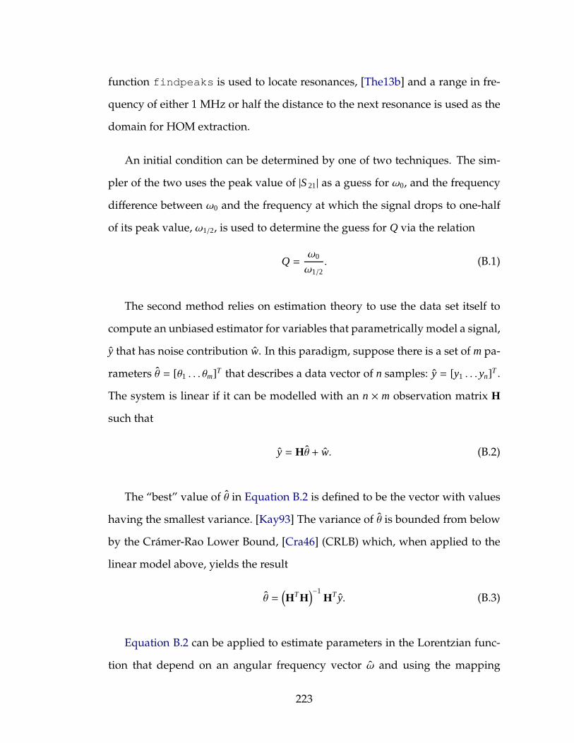
function findpeaks is used to locate resonances, [The13b] and a range in fre-
quency of either 1 MHz or half the distance to the next resonance is used as the
domain for HOM extraction.
An initial condition can be determined by one of two techniques. The sim-
pler of the two uses the peak value of |S 21| as a guess for ω0, and the frequency
difference between ω0 and the frequency at which the signal drops to one-half
of its peak value, ω1/2, is used to determine the guess for Q via the relation
Q =ω0
ω1/2. (B.1)
The second method relies on estimation theory to use the data set itself to
compute an unbiased estimator for variables that parametrically model a signal,
y that has noise contribution w. In this paradigm, suppose there is a set of m pa-
rameters θ = [θ1 . . . θm]T that describes a data vector of n samples: y = [y1 . . . yn]T .
The system is linear if it can be modelled with an n × m observation matrix H
such that
y = Hθ + w. (B.2)
The “best” value of θ in Equation B.2 is defined to be the vector with values
having the smallest variance. [Kay93] The variance of θ is bounded from below
by the Cramer-Rao Lower Bound, [Cra46] (CRLB) which, when applied to the
linear model above, yields the result
θ =(
HT H)−1
HT y. (B.3)
Equation B.2 can be applied to estimate parameters in the Lorentzian func-
tion that depend on an angular frequency vector ω and using the mapping
223
θ1 = |S 21(ω0)|, θ2 = Q−2L , and θ3 = ω0 and by rewriting Equation 4.7 revisited
in a linear form
z ≡ 1y=θ2
θ1+
1θ1
(
ω
θ3− θ3
ω
)2
, (B.4)
=
(
θ2
θ1− 2θ1
)
︸ ︷︷ ︸
φ1
+
θ23
θ1
︸︷︷︸
φ2
ω−2+
1
θ1θ23
︸ ︷︷ ︸
φ3
ω2, (B.5)
= φ1 + φ2 · ω−2+ φ3ω
2, (B.6)
where vector functions are performed element-wise, i.e. raising the vector to
the power p, is writtenyp and is equivalent to [yp1 . . . y
pn ]T . Note that a change of
variables has been performed to obtain a linear relation for an estimator φ, that
is a function of θ. The observation matrix H is then written as
(H) =
1 ω−21 ω2
1
1 ω−22 ω2
2
......
...
1 ω−2n ω2
n
. (B.7)
Applying Equation B.3 to the data set gives the estimate
φ =(
HT H)−1
HT · z, (B.8)
which can be transformed into the original parameters via
θ1 =1√φ2φ3
, (B.9)
θ2 = 2+φ1√φ2φ3
, (B.10)
θ3 =
(
φ3
φ2
)1/4
, (B.11)
224
and gives a reasonable initial condition for the optimizer. The benefit of comput-
ing an estimator in this fashion is that it is an analytic function of the data, so it
can be executed very quickly. An example of applying this method to simulated
data is presented in Figure B.1.
Though the estimated resonance in Figure B.1 doesn’t fit the curve very well
it has several benefits: First, it is an analytic function of the data, allowing for
rapid calculation. Second, the quality factor is of the proper order of magni-
tude, and horizontal and vertical scaling of the curve yield a resonable corre-
spondance to the original signal. Third, this estimator is usually a good initial
guess for an optimization-based fit of a resonance.
1550 1600 165010
−5
10−4
10−3
10−2
10−1
100
|S21|
Frequency [MHz]
SignalSignal + NoiseParameter Estimate
Figure B.1: Estimating parameters of a simulated HOM with noise. The HOMis generated with f0 = 1600 MHz and QL = 106. The CRLB yieldsan estimate of the HOM properties as fest = 1598.1 MHz and Qest =
4.1× 10⁴, which is a suitable initial condition for the optimizer.
One challenge that arises in trying to curve fit resonance data is that higher-
order mode quality factors can vary over several orders of magnitude and, due
225
to the noise in the signal, the initial condition based on Equation B.1 does not
always yield an approximation in the right range (estimation theory generally
yields superior intial QL values). To ensure the optimizer checks quality factors
over a large range, the objective function that was used in the minimizer is given
by
h(a, b, ω0; ω) =∑
10−a
√
10−2b +
(ωω0− ω0
ω
)2− y
2
. (B.12)
The quality factor of the mode is then simply QL = 10b.
B.2 Phase Fit Method
If spectral measurements measure phase information as well as magnitude of
S 21, a second method can be applied to extract HOM properties. The parameters
can also be determined from frequency vs phase information via the relation
φ(ω) = φ0 + tan−1
Q ·(
ω
ω0− ω0
ω
)
. (4.8 revisited)
This equation can be used with data measured from the network analyzer
by noting that the real, ρR(ω), and imaginary, ρI(ω) parts of Equation 4.4, trace
out a circle:
(ρR(ω) − x0)2+ (ρI(ω) − y0)
2= R2, (B.13)
where (x0, y0) is the center of the circle with radius R in the complex plane.
[SMZ89]
To obtain the phase vs frequency information, the data should be translated
so that it is centered on the origin, and rotated so that the resonant frequency
226

intersects the real axis (this allows the extent of the phase data to extend between
±π/2, which is the range of tan−1(x)). [PA98] An example of fitting the data and
transforming it to yield usable φ(ω) data is presented in Figure B.2.
−2 −1 0 1 2 3 4 5
−2
−1.5
−1
−0.5
0
0.5
1
1.5
2
2.5
Imag(S
21)
Real(S21)
DataCurve FitTransformed FitResonant frequency
Figure B.2: Illustration of the method to obtain phase vs frequency data from S 21
measurement. The network analyzer measures real an imaginaryparts of S 21, and near a resonance, the curves form circles (blue).Curve fitting yields the red curve, which fully parameterizes the cir-cles. Transforming the data yields the green curve which can beused to directly extract the phase as a function of frequency. Theblack point marks the resonant frequency. Data scale is increased bya factor of 103 in both the horizontal and vertical dimensions. Plotadapted from [Gol13].
After obtaining the parameters of the circle traced by the resonance, the
phase vs frequency data is obtained from the relationship
tanφ(ω) =ℑ(S 21)ℜ(S 21)
. (B.14)
Using Equation 4.8 revisited, the quality factor can be extracted.
Both the Lorentzian and phase fit methods yield comparable values for QL
227

for modes having their 3 dB points above the noise floor. In these cases the error
in QL is typically on the order of 20-30%. [Gol13] With modes having lower
signal-to-noise ratios, the measured QL can differ by more than 40%. In either
case, the most important figure of merit for a mode is the order of magnitude of
QL, so using both methods provides a cross check of HOM properties, which is
essential to predict the performance of the linac.
228
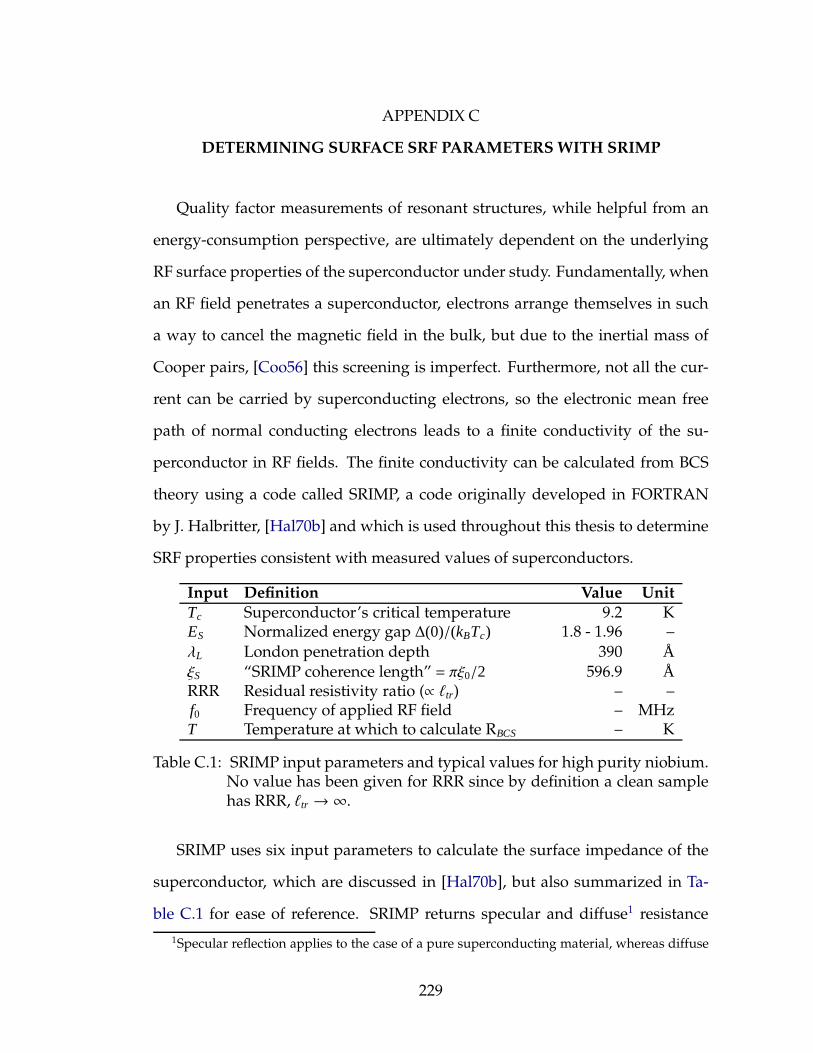
APPENDIX C
DETERMINING SURFACE SRF PARAMETERS WITH SRIMP
Quality factor measurements of resonant structures, while helpful from an
energy-consumption perspective, are ultimately dependent on the underlying
RF surface properties of the superconductor under study. Fundamentally, when
an RF field penetrates a superconductor, electrons arrange themselves in such
a way to cancel the magnetic field in the bulk, but due to the inertial mass of
Cooper pairs, [Coo56] this screening is imperfect. Furthermore, not all the cur-
rent can be carried by superconducting electrons, so the electronic mean free
path of normal conducting electrons leads to a finite conductivity of the su-
perconductor in RF fields. The finite conductivity can be calculated from BCS
theory using a code called SRIMP, a code originally developed in FORTRAN
by J. Halbritter, [Hal70b] and which is used throughout this thesis to determine
SRF properties consistent with measured values of superconductors.
Input Definition Value Unit
Tc Superconductor’s critical temperature 9.2 KES Normalized energy gap ∆(0)/(kBTc) 1.8 - 1.96 –
λL London penetration depth 390 ÅξS “SRIMP coherence length” = πξ0/2 596.9 ÅRRR Residual resistivity ratio (∝ ℓtr) – –f0 Frequency of applied RF field – MHzT Temperature at which to calculate RBCS – K
Table C.1: SRIMP input parameters and typical values for high purity niobium.No value has been given for RRR since by definition a clean samplehas RRR, ℓtr → ∞.
SRIMP uses six input parameters to calculate the surface impedance of the
superconductor, which are discussed in [Hal70b], but also summarized in Ta-
ble C.1 for ease of reference. SRIMP returns specular and diffuse1 resistance
1Specular reflection applies to the case of a pure superconducting material, whereas diffuse
229
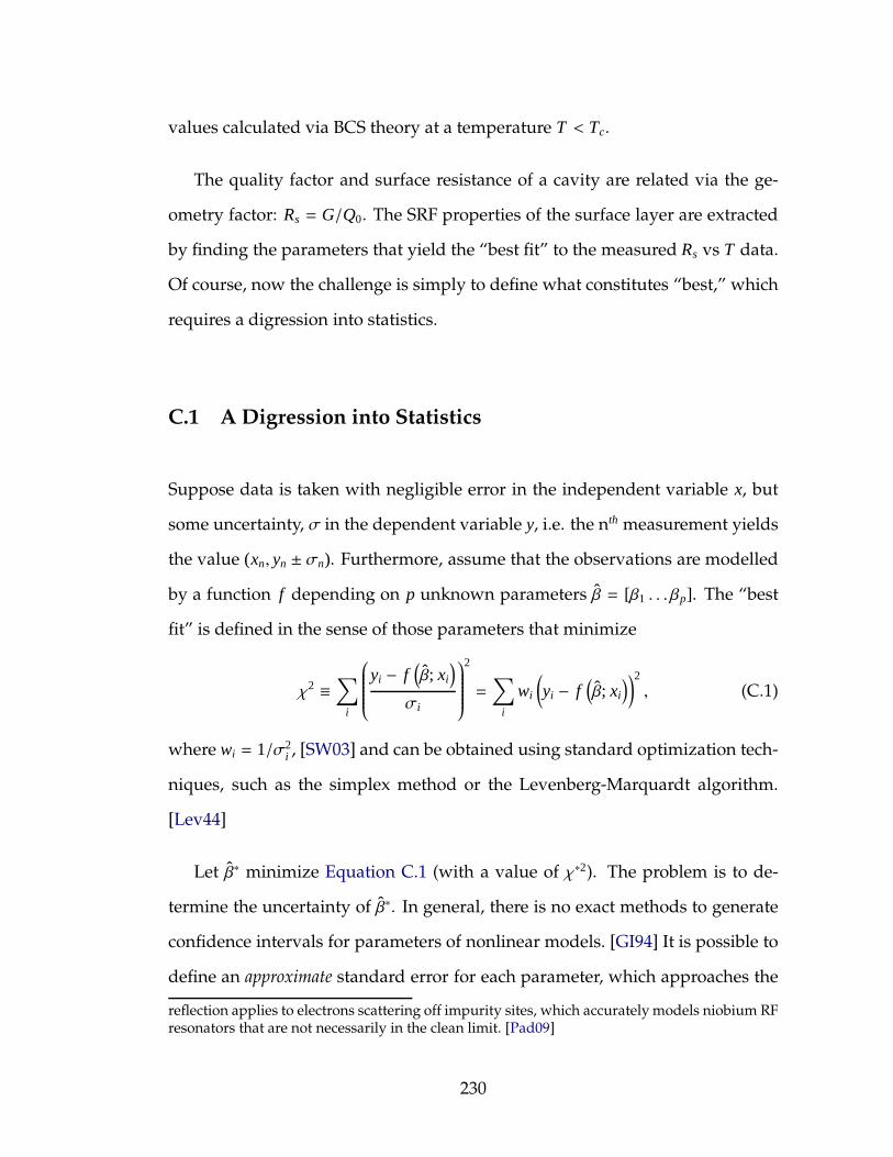
values calculated via BCS theory at a temperature T < Tc.
The quality factor and surface resistance of a cavity are related via the ge-
ometry factor: Rs = G/Q0. The SRF properties of the surface layer are extracted
by finding the parameters that yield the “best fit” to the measured Rs vs T data.
Of course, now the challenge is simply to define what constitutes “best,” which
requires a digression into statistics.
C.1 A Digression into Statistics
Suppose data is taken with negligible error in the independent variable x, but
some uncertainty, σ in the dependent variable y, i.e. the nth measurement yields
the value (xn, yn ± σn). Furthermore, assume that the observations are modelled
by a function f depending on p unknown parameters β = [β1 . . . βp]. The “best
fit” is defined in the sense of those parameters that minimize
χ2 ≡∑
i
yi − f(
β; xi
)
σi
2
=
∑
i
wi
(
yi − f(
β; xi
))2
, (C.1)
where wi = 1/σ2i , [SW03] and can be obtained using standard optimization tech-
niques, such as the simplex method or the Levenberg-Marquardt algorithm.
[Lev44]
Let β∗ minimize Equation C.1 (with a value of χ∗2). The problem is to de-
termine the uncertainty of β∗. In general, there is no exact methods to generate
confidence intervals for parameters of nonlinear models. [GI94] It is possible to
define an approximate standard error for each parameter, which approaches the
reflection applies to electrons scattering off impurity sites, which accurately models niobium RFresonators that are not necessarily in the clean limit. [Pad09]
230
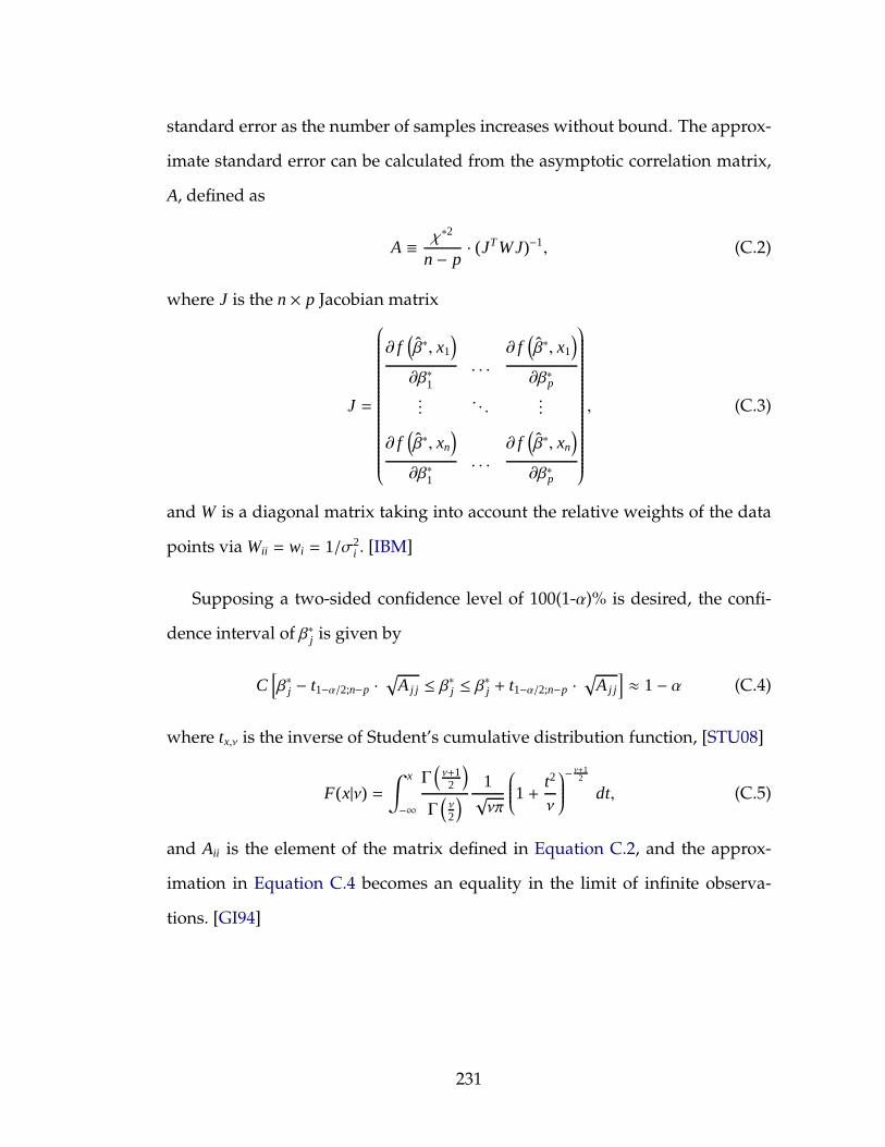
standard error as the number of samples increases without bound. The approx-
imate standard error can be calculated from the asymptotic correlation matrix,
A, defined as
A ≡ χ∗2
n − p· (JT WJ)−1, (C.2)
where J is the n × p Jacobian matrix
J =
∂ f(
β∗, x1
)
∂β∗1. . .
∂ f(
β∗, x1
)
∂β∗p...
. . ....
∂ f(
β∗, xn
)
∂β∗1. . .
∂ f(
β∗, xn
)
∂β∗p
, (C.3)
and W is a diagonal matrix taking into account the relative weights of the data
points via Wii = wi = 1/σ2i . [IBM]
Supposing a two-sided confidence level of 100(1-α)% is desired, the confi-
dence interval of β∗j is given by
C[
β∗j − t1−α/2;n−p ·√
A j j ≤ β∗j ≤ β∗j + t1−α/2;n−p ·√
A j j
]
≈ 1− α (C.4)
where tx,ν is the inverse of Student’s cumulative distribution function, [STU08]
F(x|ν) =∫ x
−∞
Γ
(ν+12
)
Γ
(ν2
)1√νπ
1+t2
ν
− ν+12
dt, (C.5)
and Aii is the element of the matrix defined in Equation C.2, and the approx-
imation in Equation C.4 becomes an equality in the limit of infinite observa-
tions. [GI94]
231
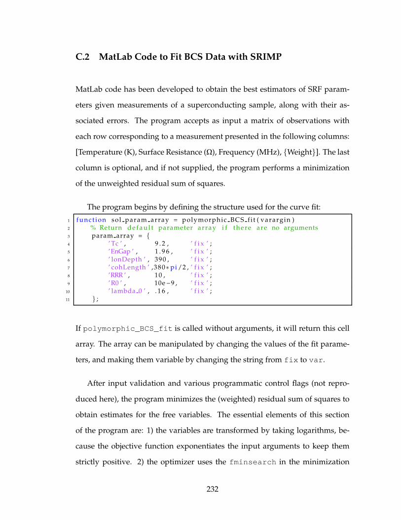
C.2 MatLab Code to Fit BCS Data with SRIMP
MatLab code has been developed to obtain the best estimators of SRF param-
eters given measurements of a superconducting sample, along with their as-
sociated errors. The program accepts as input a matrix of observations with
each row corresponding to a measurement presented in the following columns:
[Temperature (K), Surface Resistance (Ω), Frequency (MHz), Weight]. The last
column is optional, and if not supplied, the program performs a minimization
of the unweighted residual sum of squares.
The program begins by defining the structure used for the curve fit:
1 func t ion sol param array = polymorphic BCS f i t ( varargin )2 % Return d e f a u l t parameter array i f there are no arguments3 param array = 4 ’ Tc ’ , 9 . 2 , ’ f i x ’ ;5 ’EnGap ’ , 1 . 9 6 , ’ f i x ’ ;6 ’ lonDepth ’ , 390 , ’ f i x ’ ;7 ’ cohLength ’ ,380∗ pi /2 , ’ f i x ’ ;8 ’RRR ’ , 10 , ’ f i x ’ ;9 ’R0 ’ , 10e−9 , ’ f i x ’ ;
10 ’ lambda 0 ’ , . 1 6 , ’ f i x ’ ;11 ;
If polymorphic_BCS_fit is called without arguments, it will return this cell
array. The array can be manipulated by changing the values of the fit parame-
ters, and making them variable by changing the string from fix to var.
After input validation and various programmatic control flags (not repro-
duced here), the program minimizes the (weighted) residual sum of squares to
obtain estimates for the free variables. The essential elements of this section
of the program are: 1) the variables are transformed by taking logarithms, be-
cause the objective function exponentiates the input arguments to keep them
strictly positive. 2) the optimizer uses the fminsearch in the minimization
232
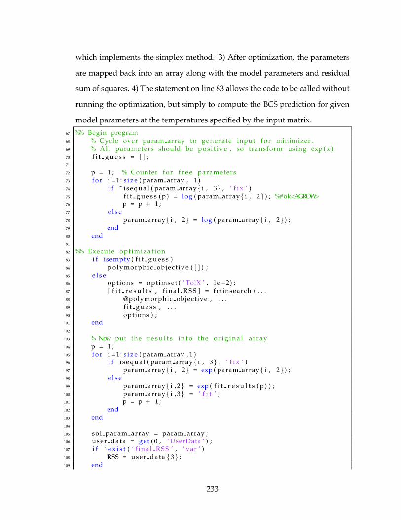
which implements the simplex method. 3) After optimization, the parameters
are mapped back into an array along with the model parameters and residual
sum of squares. 4) The statement on line 83 allows the code to be called without
running the optimization, but simply to compute the BCS prediction for given
model parameters at the temperatures specified by the input matrix.
67 %% Begin program68 % Cycle over param array to generate input f o r minimizer .69 % All parameters should be p o s i t i v e , so transform using exp ( x )70 f i t g u e s s = [ ] ;71
72 p = 1 ; % Counter f o r f r e e parameters73 f o r i =1 : s i z e ( param array , 1 )74 i f ˜ i s e q u a l ( param array i , 3 , ’ f i x ’ )75 f i t g u e s s ( p ) = log ( param array i , 2 ) ; %#ok<AGROW>76 p = p + 1 ;77 e l s e78 param array i , 2 = log ( param array i , 2 ) ;79 end80 end81
82 %% Execute opt imiz a t ion83 i f isempty ( f i t g u e s s )84 polymorphic ob jec t ive ( [ ] ) ;85 e l s e86 options = optimset ( ’ TolX ’ , 1e−2) ;87 [ f i t r e s u l t s , f i n a l R S S ] = fminsearch ( . . .88 @polymorphic objective , . . .89 f i t g u e s s , . . .90 options ) ;91 end92
93 % Now put the r e s u l t s i n t o the o r i g i n a l array94 p = 1 ;95 f o r i =1 : s i z e ( param array , 1 )96 i f i s e q u a l ( param array i , 3 , ’ f i x ’ )97 param array i , 2 = exp ( param array i , 2 ) ;98 e l s e99 param array i , 2 = exp ( f i t r e s u l t s ( p ) ) ;
100 param array i , 3 = ’ f i t ’ ;101 p = p + 1 ;102 end103 end104
105 sol param array = param array ;106 user da ta = get ( 0 , ’ UserData ’ ) ;107 i f ˜ e x i s t ( ’ f i n a l R S S ’ , ’ var ’ )108 RSS = user da ta 3 ;109 end
233
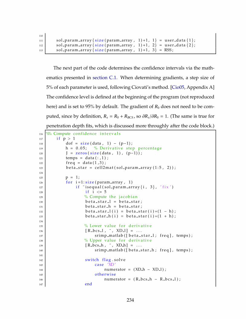
110
111 sol param array s i z e ( param array , 1 ) +1 , 1 = user da ta 1 ;112 sol param array s i z e ( param array , 1 ) +1 , 2 = user da ta 2 ;113 sol param array s i z e ( param array , 1 ) +1 , 3 = RSS ;
The next part of the code determines the confidence intervals via the math-
ematics presented in section C.1. When determining gradients, a step size of
5% of each parameter is used, following Ciovati’s method. [Cio05, Appendix A]
The confidence level is defined at the beginning of the program (not reproduced
here) and is set to 95% by default. The gradient of R0 does not need to be com-
puted, since by definition, Rs = R0 + RBCS , so ∂Rs/∂R0 = 1. (The same is true for
penetration depth fits, which is discussed more throughly after the code block.)
116 %% Compute conf idence i n t e r v a l s117 i f p > 1118 dof = s i z e ( data , 1 ) − ( p−1) ;119 h = 0 . 0 5 ; % Der iva t ive step percentage120 J = zeros ( s i z e ( data , 1 ) , ( p−1) ) ;121 temps = data ( : , 1 ) ;122 f r e q = data ( 1 , 3 ) ;123 b e t a s t a r = ce l l2 ma t ( sol param array ( 1 : 5 , 2 ) ) ;124
125 p = 1 ;126 f o r i =1 : s i z e ( param array , 1 )127 i f ˜ i s e q u a l ( sol param array i , 3 , ’ f i x ’ )128 i f i <= 5129 % Compute the j a c o b i a n130 b e t a s t a r l = b e t a s t a r ;131 b e t a s t a r h = b e t a s t a r ;132 b e t a s t a r l ( i ) = b e t a s t a r ( i ) ∗ (1 − h ) ;133 b e t a s t a r h ( i ) = b e t a s t a r ( i ) ∗ (1 + h ) ;134
135 % Lower value f o r d e r i v a t i v e136 [ R bcs l , ˜ , XD l ] = . . .137 srimp matlab ( [ b e t a s t a r l ; f r e q ] , temps ) ;138 % Upper value f o r d e r i v a t i v e139 [ R bcs h , ˜ , XD h ] = . . .140 srimp matlab ( [ b e t a s t a r h ; f r e q ] , temps ) ;141
142 switch f l a g . so lve143 case ’XD ’144 numerator = ( XD h − XD l ) ;145 otherwise146 numerator = ( R bcs h − R b c s l ) ;147 end
234
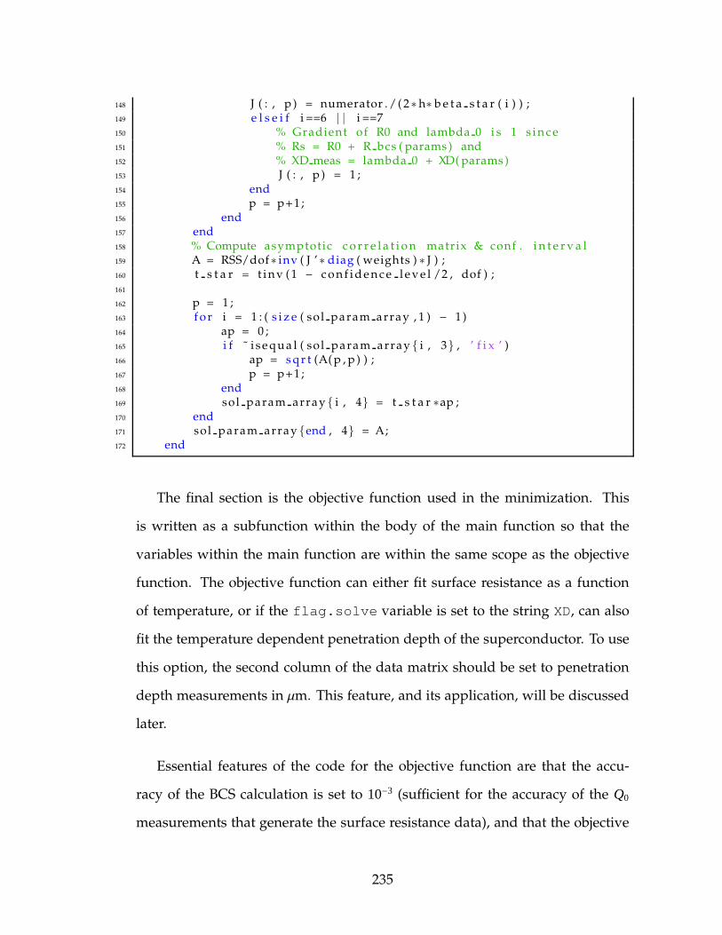
148 J ( : , p ) = numerator . / ( 2∗h∗ b e t a s t a r ( i ) ) ;149 e l s e i f i ==6 | | i ==7150 % Gradient of R0 and lambda 0 i s 1 s i n c e151 % Rs = R0 + R bcs ( params ) and152 % XD meas = lambda 0 + XD( params )153 J ( : , p ) = 1 ;154 end155 p = p+1;156 end157 end158 % Compute asymptotic c o r r e l a t i o n matrix & conf . i n t e r v a l159 A = RSS/dof∗ inv ( J ’∗ diag ( weights ) ∗ J ) ;160 t s t a r = t i n v (1 − c o n f i d e n c e l e v e l /2 , dof ) ;161
162 p = 1 ;163 f o r i = 1 : ( s i z e ( sol param array , 1 ) − 1 )164 ap = 0 ;165 i f ˜ i s e q u a l ( sol param array i , 3 , ’ f i x ’ )166 ap = s q r t (A( p , p ) ) ;167 p = p+1;168 end169 sol param array i , 4 = t s t a r ∗ap ;170 end171 sol param array end , 4 = A;172 end
The final section is the objective function used in the minimization. This
is written as a subfunction within the body of the main function so that the
variables within the main function are within the same scope as the objective
function. The objective function can either fit surface resistance as a function
of temperature, or if the flag.solve variable is set to the string XD, can also
fit the temperature dependent penetration depth of the superconductor. To use
this option, the second column of the data matrix should be set to penetration
depth measurements in µm. This feature, and its application, will be discussed
later.
Essential features of the code for the objective function are that the accu-
racy of the BCS calculation is set to 10−3 (sufficient for the accuracy of the Q0
measurements that generate the surface resistance data), and that the objective
235
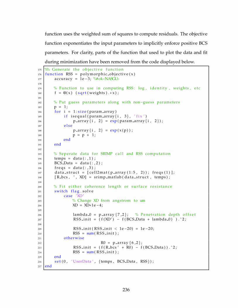
function uses the weighted sum of squares to compute residuals. The objective
function exponentiates the input parameters to implicitly enforce positive BCS
parameters. For clarity, parts of the function that used to plot the data and fit
during minimization have been removed from the code displayed below.
175 %% Generate the o b j e c t i v e funct ion176 func t ion RSS = polymorphic ob jec t ive ( x )177 accuracy = 1e −3 ; %#ok<NASGU>178
179 % Function to use in computing RSS : log , i d e n t i t y , weights , e t c180 f = @( x ) ( s q r t ( weights ) .∗ x ) ;181
182 % Put guess parameters along with non−guess parameters183 p = 1 ;184 f o r i = 1 : s i z e ( param array )185 i f i s e q u a l ( param array i , 3 , ’ f i x ’ )186 p array i , 2 = exp ( param array i , 2 ) ;187 e l s e188 p array i , 2 = exp ( x ( p) ) ;189 p = p + 1 ;190 end191 end192
193 % Seperate data f o r SRIMP c a l l and RSS computation194 temps = data ( : , 1 ) ;195 BCS Data = data ( : , 2 ) ;196 f r e q s = data ( : , 3 ) ;197 d a t a s t r u c t = [ ce l l2 ma t ( p array ( 1 : 5 , 2 ) ) ; f r e q s ( 1 ) ] ;198 [ R bcs , ˜ , XD] = srimp matlab ( d a t a s t r u c t , temps ) ;199
200 % F i t e i t h e r coherence length or s u r f a c e r e s i s t a n c e201 switch f l a g . so lve202 case ’XD ’203 % Change XD from angstrom to um204 XD = XD∗1e −4 ;205
206 lambda 0 = p array 7 , 2 ; % Penetra t ion depth o f f s e t207 R S S i n i t = ( f (XD’ ) − f ( BCS Data + lambda 0 ) ) . ˆ 2 ;208
209 R S S i n i t ( R S S i n i t < 1e−20) = 1e −20 ;210 RSS = sum( R S S i n i t ) ;211 otherwise212 R0 = p array 6 , 2 ;213 R S S i n i t = ( f ( R bcs ’ + R0 ) − f ( BCS Data ) ) . ˆ 2 ;214 RSS = sum( R S S i n i t ) ;215 end216 s e t ( 0 , ’ UserData ’ , temps , BCS Data , RSS ) ;217 end
236
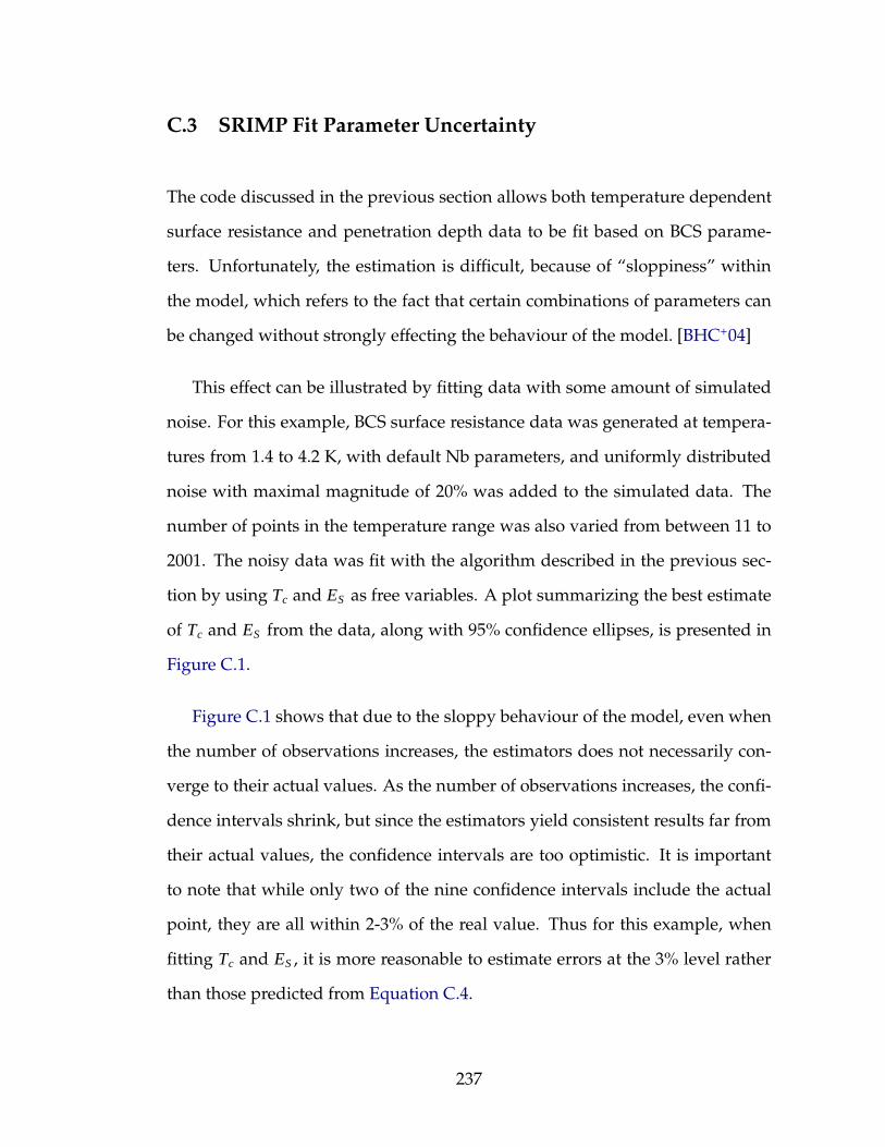
C.3 SRIMP Fit Parameter Uncertainty
The code discussed in the previous section allows both temperature dependent
surface resistance and penetration depth data to be fit based on BCS parame-
ters. Unfortunately, the estimation is difficult, because of “sloppiness” within
the model, which refers to the fact that certain combinations of parameters can
be changed without strongly effecting the behaviour of the model. [BHC+04]
This effect can be illustrated by fitting data with some amount of simulated
noise. For this example, BCS surface resistance data was generated at tempera-
tures from 1.4 to 4.2 K, with default Nb parameters, and uniformly distributed
noise with maximal magnitude of 20% was added to the simulated data. The
number of points in the temperature range was also varied from between 11 to
2001. The noisy data was fit with the algorithm described in the previous sec-
tion by using Tc and ES as free variables. A plot summarizing the best estimate
of Tc and ES from the data, along with 95% confidence ellipses, is presented in
Figure C.1.
Figure C.1 shows that due to the sloppy behaviour of the model, even when
the number of observations increases, the estimators does not necessarily con-
verge to their actual values. As the number of observations increases, the confi-
dence intervals shrink, but since the estimators yield consistent results far from
their actual values, the confidence intervals are too optimistic. It is important
to note that while only two of the nine confidence intervals include the actual
point, they are all within 2-3% of the real value. Thus for this example, when
fitting Tc and ES , it is more reasonable to estimate errors at the 3% level rather
than those predicted from Equation C.4.
237
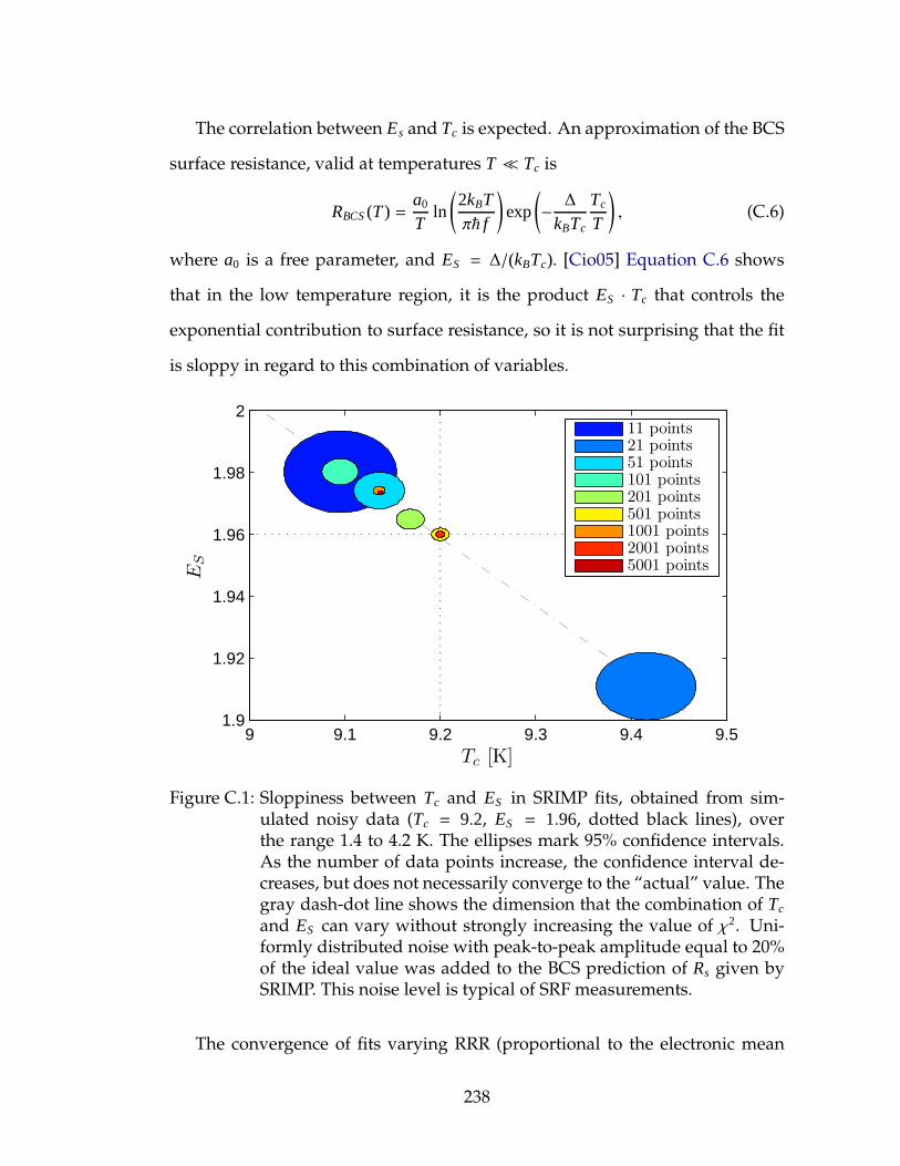
The correlation between Es and Tc is expected. An approximation of the BCS
surface resistance, valid at temperatures T ≪ Tc is
RBCS (T ) =a0
Tln
(
2kBTπ~ f
)
exp
(
− ∆kBTc
Tc
T
)
, (C.6)
where a0 is a free parameter, and ES = ∆/(kBTc). [Cio05] Equation C.6 shows
that in the low temperature region, it is the product ES · Tc that controls the
exponential contribution to surface resistance, so it is not surprising that the fit
is sloppy in regard to this combination of variables.
9 9.1 9.2 9.3 9.4 9.51.9
1.92
1.94
1.96
1.98
2
ES
Tc [K]
11 points21 points51 points101 points201 points501 points1001 points2001 points5001 points
Figure C.1: Sloppiness between Tc and ES in SRIMP fits, obtained from sim-ulated noisy data (Tc = 9.2, ES = 1.96, dotted black lines), overthe range 1.4 to 4.2 K. The ellipses mark 95% confidence intervals.As the number of data points increase, the confidence interval de-creases, but does not necessarily converge to the “actual” value. Thegray dash-dot line shows the dimension that the combination of Tc
and ES can vary without strongly increasing the value of χ2. Uni-formly distributed noise with peak-to-peak amplitude equal to 20%of the ideal value was added to the BCS prediction of Rs given bySRIMP. This noise level is typical of SRF measurements.
The convergence of fits varying RRR (proportional to the electronic mean
238
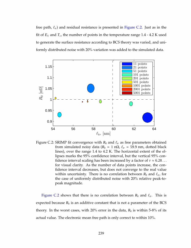
free path, ℓtr) and residual resistance is presented in Figure C.2. Just as in the
fit of ES and Tc, the number of points in the temperature range 1.4 - 4.2 K used
to generate the surface resistance according to BCS theory was varied, and uni-
formly distributed noise with 20% variation was added to the simulated data.
54 56 58 60 62 64
0.9
0.95
1
1.05
1.1
1.15
ℓtr [nm]
R0
[nΩ
]
11 points21 points51 points101 points201 points501 points1001 points2001 points5001 points
Figure C.2: SRIMP fit convergence with R0 and ℓtr as free parameters obtainedfrom simulated noisy data (R0 = 1 nΩ, ℓtr = 59.9 nm, dotted blacklines), over the range 1.4 to 4.2 K. The horizontal extent of the el-lipses marks the 95% confidence interval, but the vertical 95% con-fidence interval scaling has been increased by a factor of τ ≈ 6.28. . .for visual clarity. As the number of data points increase, the con-fidence interval decreases, but does not converge to the real valuewithin uncertainty. There is no correlation between R0 and ℓtr, forthe case of uniformly distributed noise with 20% relative peak-to-peak magnitude.
Figure C.2 shows that there is no correlation between R0 and ℓtr. This is
expected because R0 is an additive constant that is not a parameter of the BCS
theory. In the worst cases, with 20% error in the data, R0 is within 5-8% of its
actual value. The electronic mean free path is only correct to within 10%.
239

To quantify the difference between the propagated error calculated from the
asymptotic correlation matrix and the actual difference between fit parameters
and the real underlying values, simulations were run varying both the number
of points and the noise level. As before, the parameters used to generate BCS
data was that of standard Nb, with electronic mean free path of 59.9 nm, and
a residual resistance of 1 nΩ. Fits with 2 degrees of freedom were performed,
either with R0 and ℓtr as free parameters or with ES and Tc being varied.
In the following figures, an additional factor, ζ has been introduced, that
measures by what factor the 95% confidence interval computed via Equation C.4
would have to be increased to include the actual value of the SRF parameter.
Mathematically,
ζi ≡|β∗i − βi|
t0.975;n−p ·√
Aii
, (C.7)
where in this case β∗i is the best estimate of the free parameter βi, and Aii is the
diagonal element of the asymptotic correlation matrix corresponding to βi.
First, fits with only ℓtr and R0 as free parameters were performed at three dif-
ferent noise levels. Figure C.3 shows the accuracy of ℓtr as the number of points
in the data sample increases. It is essential to note that even with low numbers
of observations, and large noise, ℓ∗tr is accurate to better than 8%. In contrast, ζ
is consistently above unity–meaning the confidence interval is underestimated–
even for large numbers of points.
The same information for R0 is displayed in Figure C.4. In this case, the worst
case relative error is 9%, but as noise levels decrease, the error can be <1%. As
in the case of ℓtr, ζ does not converge to unity at large number of observations,
but remains around 10 for most noise levels.
240

10−3
10−2
10−1
|Rel
ative
Err
or|
20% 10% 5%
101
102
100
101
102
Number of points
ζ,ℓ t
r
Figure C.3: SRIMP fit relative error of ℓtr with R0 and ℓtr as free parameters ob-tained from simulated noisy data (R0 = 1 nΩ, ℓtr = 59.9 nm), from1.4 to 4.2 K. Top: Absolute value of relative error in ℓtr. Bottom: ζas defined in Equation C.7 as a function of number of data pointsin the observation for various noise levels. Uniformly distributednoise had relative peak-to-peak magnitude of 5, 10, and 20%.
10−3
10−2
10−1
|Rel
ative
Err
or|
20% 10% 5%
101
102
100
101
102
Number of points
ζ,R
0
Figure C.4: SRIMP fit relative error of R0 with R0 and ℓtr as free parameters. Top:Absolute value of relative error in R0. Bottom: ζ as defined in Equa-tion C.7 as a function of number of observations for various noiselevels. Uniformly distributed noise had relative peak-to-peak mag-nitude of 5, 10, and 20%.
241
Next, fits varying Tc and ES were performed at three different noise levels.
Figure C.5 shows the accuracy of Tc as the number of points in the data sample
increases. It is essential to note that even with low numbers of observations,
and large noise, T ∗c is accurate to better than 2%. In contrast, the estimate for
the confidence interval is consistently more than a factor of 2 too small, even for
large numbers of points.
10−3
10−2
10−1
|Rel
ative
Err
or,
Tc|
20% 10% 5%
101
102
10−1
100
101
Number of points
ζ,T
c
Figure C.5: SRIMP fit relative error of Tc with Tc and ES as free parameters ob-tained from simulated noisy data (R0 = 1 nΩ, ℓtr = 59.9 nm), from1.4 to 4.2 K. Top: Absolute value of relative error in Tc. Bottom: ζas defined in Equation C.7 as a function of number of observationsfor various noise levels. Uniformly distributed noise had relativepeak-to-peak magnitude of 5, 10, and 20%.
The results from fitting ES is displayed in Figure C.6. In this case, the worst
case relative error is ≈ 7%, but as noise levels decrease, the error can be within
2%. As in the case of the other parameters investigated, ζ does not converge to
unity at large number of observations for ES .
242
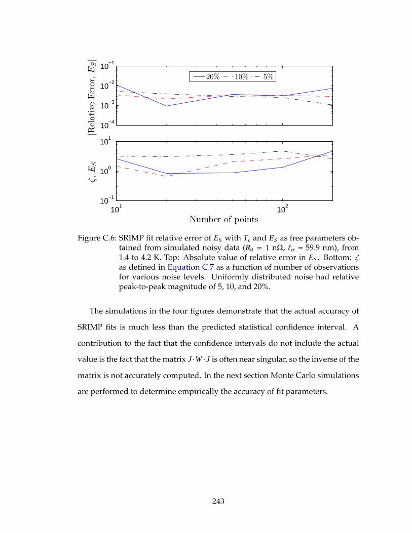
10−4
10−3
10−2
10−1
|Rel
ative
Err
or,
ES|
20% 10% 5%
101
102
10−1
100
101
Number of points
ζ,E
S
Figure C.6: SRIMP fit relative error of ES with Tc and ES as free parameters ob-tained from simulated noisy data (R0 = 1 nΩ, ℓtr = 59.9 nm), from1.4 to 4.2 K. Top: Absolute value of relative error in ES . Bottom: ζas defined in Equation C.7 as a function of number of observationsfor various noise levels. Uniformly distributed noise had relativepeak-to-peak magnitude of 5, 10, and 20%.
The simulations in the four figures demonstrate that the actual accuracy of
SRIMP fits is much less than the predicted statistical confidence interval. A
contribution to the fact that the confidence intervals do not include the actual
value is the fact that the matrix J ·W ·J is often near singular, so the inverse of the
matrix is not accurately computed. In the next section Monte Carlo simulations
are performed to determine empirically the accuracy of fit parameters.
243
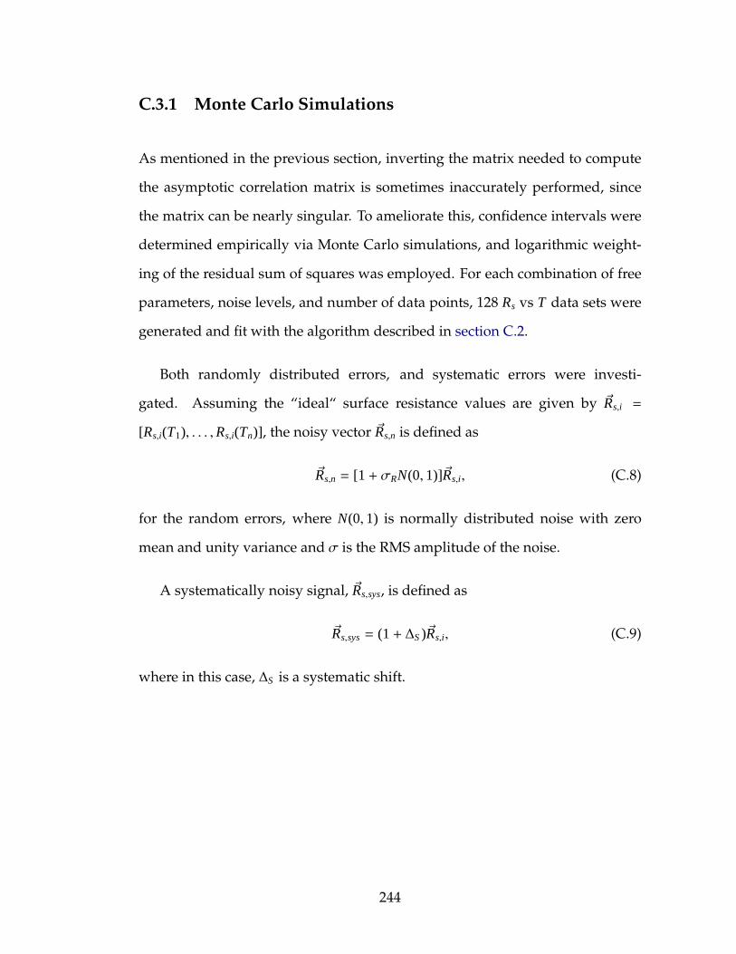
C.3.1 Monte Carlo Simulations
As mentioned in the previous section, inverting the matrix needed to compute
the asymptotic correlation matrix is sometimes inaccurately performed, since
the matrix can be nearly singular. To ameliorate this, confidence intervals were
determined empirically via Monte Carlo simulations, and logarithmic weight-
ing of the residual sum of squares was employed. For each combination of free
parameters, noise levels, and number of data points, 128 Rs vs T data sets were
generated and fit with the algorithm described in section C.2.
Both randomly distributed errors, and systematic errors were investi-
gated. Assuming the “ideal“ surface resistance values are given by ~Rs,i =
[Rs,i(T1), . . . ,Rs,i(Tn)], the noisy vector ~Rs,n is defined as
~Rs,n = [1 + σRN(0, 1)]~Rs,i, (C.8)
for the random errors, where N(0, 1) is normally distributed noise with zero
mean and unity variance and σ is the RMS amplitude of the noise.
A systematically noisy signal, ~Rs,sys, is defined as
~Rs,sys = (1+ ∆S )~Rs,i, (C.9)
where in this case, ∆S is a systematic shift.
244

SRIMP Fits with 4-degrees of Freedom
Histograms presenting the distribution of parameter estimates for a fit with 4
degrees of freedom (Tc, ES , ℓtr and R0) of signals with random noise are pre-
sented in Figures C.7, C.8, C.9, and C.10. The nominal values of the super-
conducting RF layer are Tc = 9.2 K, ES = 1.96, ℓtr = 16.7 nm, R0=10 nΩ. The
histograms show the resulting best fit parameters for various combinations of
the number points taken between 1.4 and 4.2 K and random noise levels.
The histograms demonstrate that in most cases, the mean of the estimates
are very close to the actual value of the parameter. There are a few outliers
that strongly increase the standard deviation of the estimates. One exception is
that the fits of ℓtr suggest that the underlying distribution is skewed, and has a
long, one-sided tail, meaning that a normal distribution may not be a suitable
representation of the data. Figure C.11 shows the distribution of ℓtr compared
with a gamma probability distribution.
245
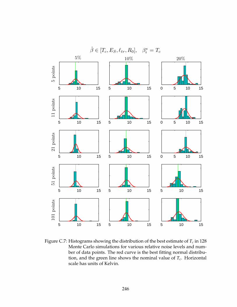
5 10 15
5poin
ts5%
5 10 15
10%
0 5 10 15
20%
5 10 15
11
poin
ts
5 10 15 0 5 10 15
5 10 15
21
poin
ts
5 10 15 0 5 10 15
5 10 15
51
poin
ts
5 10 15 5 10 15
5 10 15
101
poin
ts
5 10 15
β ∈ [Tc,ES , ℓtr,R0], β∗i = Tc
5 10 15
Figure C.7: Histograms showing the distribution of the best estimate of Tc in 128Monte Carlo simulations for various relative noise levels and num-ber of data points. The red curve is the best fitting normal distribu-tion, and the green line shows the nominal value of Tc. Horizontalscale has units of Kelvin.
246
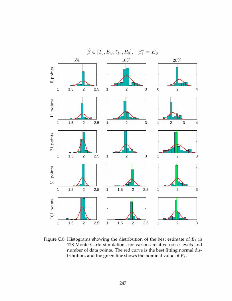
1 1.5 2 2.5
5poin
ts
5%
1 2 3
10%
0 2 4
20%
1 1.5 2 2.5
11
poin
ts
1 2 3 1 2 3 4
1 1.5 2 2.5
21
poin
ts
1 2 3 1 2 3
1 1.5 2 2.5
51
poin
ts
1 1.5 2 2.5 1 2 3
1 1.5 2 2.5
101
poin
ts
1 1.5 2 2.5
β ∈ [Tc,ES , ℓtr,R0], β∗i = ES
1 2 3
Figure C.8: Histograms showing the distribution of the best estimate of ES in128 Monte Carlo simulations for various relative noise levels andnumber of data points. The red curve is the best fitting normal dis-tribution, and the green line shows the nominal value of ES .
247
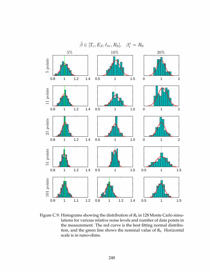
0.8 1 1.2 1.4
5poin
ts5%
0.5 1 1.5
10%
0 1 2
20%
0.8 1 1.2 1.4
11
poin
ts
0.5 1 1.5 0 1 2
0.8 1 1.2 1.4
21
poin
ts
0.5 1 1.5 0 1 2
0.8 1 1.2 1.4
51
poin
ts
0.5 1 1.5 0.5 1 1.5
0.9 1 1.1 1.2
101
poin
ts
0.8 1 1.2 1.4
β ∈ [Tc,ES , ℓtr,R0], β∗i = R0
0.5 1 1.5
Figure C.9: Histograms showing the distribution of R0 in 128 Monte Carlo simu-lations for various relative noise levels and number of data points inthe measurement. The red curve is the best fitting normal distribu-tion, and the green line shows the nominal value of R0. Horizontalscale is in nano-ohms.
248
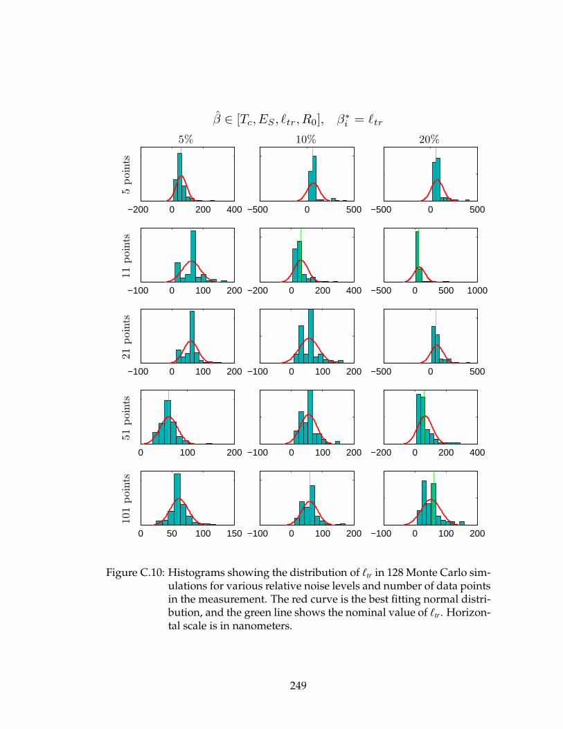
−200 0 200 400
5poin
ts5%
−500 0 500
10%
−500 0 500
20%
−100 0 100 200
11
poin
ts
−200 0 200 400 −500 0 500 1000
−100 0 100 200
21
poin
ts
−100 0 100 200 −500 0 500
0 100 200
51
poin
ts
−100 0 100 200 −200 0 200 400
0 50 100 150
101
poin
ts
−100 0 100 200
β ∈ [Tc,ES , ℓtr,R0], β∗i = ℓtr
−100 0 100 200
Figure C.10: Histograms showing the distribution of ℓtr in 128 Monte Carlo sim-ulations for various relative noise levels and number of data pointsin the measurement. The red curve is the best fitting normal distri-bution, and the green line shows the nominal value of ℓtr. Horizon-tal scale is in nanometers.
249
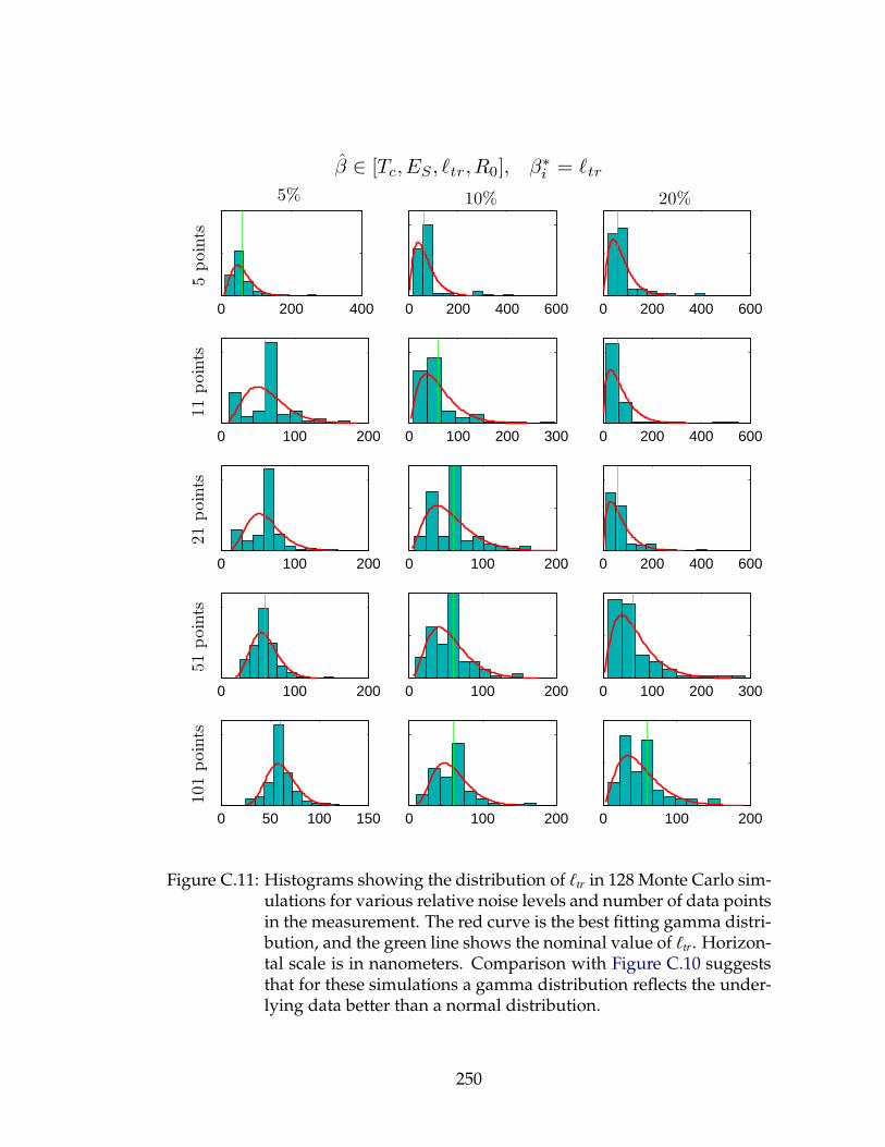
0 200 400
5poin
ts5%
0 200 400 600
10%
0 200 400 600
20%
0 100 200
11
poin
ts
0 100 200 300 0 200 400 600
0 100 200
21
poin
ts
0 100 200 0 200 400 600
0 100 200
51
poin
ts
0 100 200 0 100 200 300
0 50 100 150
101
poin
ts
0 100 200
β ∈ [Tc,ES , ℓtr,R0], β∗i = ℓtr
0 100 200
Figure C.11: Histograms showing the distribution of ℓtr in 128 Monte Carlo sim-ulations for various relative noise levels and number of data pointsin the measurement. The red curve is the best fitting gamma distri-bution, and the green line shows the nominal value of ℓtr. Horizon-tal scale is in nanometers. Comparison with Figure C.10 suggeststhat for these simulations a gamma distribution reflects the under-lying data better than a normal distribution.
250
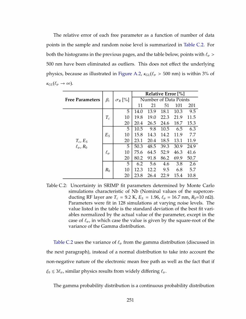
The relative error of each free parameter as a function of number of data
points in the sample and random noise level is summarized in Table C.2. For
both the histograms in the previous pages, and the table below, points with ℓtr >
500 nm have been eliminated as outliers. This does not effect the underlying
physics, because as illustrated in Figure A.2, κGL(ℓtr > 500 nm) is within 3% of
κGL(ℓtr →∞).
Free Parameters βi σR [%]Relative Error [%]
Number of Data Points11 21 51 101 201
Tc, ES
ℓtr, R0
Tc
5 14.0 13.9 18.1 10.3 9.510 19.8 19.0 22.3 21.9 11.520 20.4 26.5 24.6 18.7 15.3
ES
5 10.5 9.8 10.5 6.5 6.310 15.8 14.3 14.2 11.9 7.720 23.1 20.4 18.5 13.1 11.9
ℓtr
5 50.3 48.5 39.3 30.9 24.910 75.6 64.5 52.9 46.3 41.620 80.2 91.8 86.2 69.9 50.7
R0
5 6.2 5.6 4.6 3.8 2.610 12.3 12.2 9.5 6.8 5.720 23.8 26.4 22.9 15.4 10.8
Table C.2: Uncertainty in SRIMP fit parameters determined by Monte Carlosimulations characteristic of Nb (Nominal values of the supercon-ducting RF layer are Tc = 9.2 K, ES = 1.96, ℓtr = 16.7 nm, R0=10 nΩ).Parameters were fit in 128 simulations at varying noise levels. Thevalue listed in the table is the standard deviation of the best fit vari-ables normalized by the actual value of the parameter, except in thecase of ℓtr, in which case the value is given by the square-root of thevariance of the Gamma distribution.
Table C.2 uses the variance of ℓtr from the gamma distribution (discussed in
the next paragraph), instead of a normal distribution to take into account the
non-negative nature of the electronic mean free path as well as the fact that if
ξ0 . 3ℓtr, similar physics results from widely differing ℓtr.
The gamma probability distribution is a continuous probability distribution
251

defined on the support x ∈ [0,∞), characterized by a shape parameter, k and
scale parameter, θ, with the form
f (k, θ; x) =1
θkΓ(k)xk−1 exp
(
− xθ
)
, (C.10)
where Γ(k) is the gamma function, or generalized factorial function. [Haz88] The
mean of this distribution is given by kθ and the variance is kθ2.
Systematic errors were also computed by applying Equation C.9 to ideal data
with ∆S ∈ [−0.15, 0.15]. The results are presented in Figure C.12.
−10 0 10−40
−20
0
20
40
Err
or
inT
c[%
]
5 points11 points21 points
−10 0 10−30
−20
−10
0
10
Err
or
inE
S[%
]
−10 0 10−100
0
100
Err
or
inℓ t
r[%
]
Systematic Error [%]−10 0 10
−20
0
20
Err
or
inR
0[%
]
Systematic Error [%]
Figure C.12: Relative error in SRIMP fits as a function of systematic error for 4degrees of freedom for typical niobium. Horizontal axes are thevalues of ∆S used in Equation C.9 which range between ±15%. Thejagged appearance of the signals is due the fact that the parametersare not uncorrelated.
252
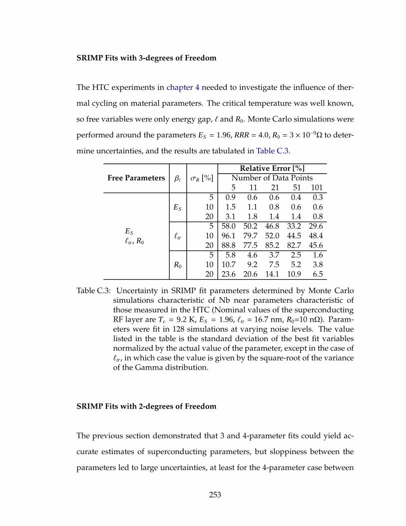
SRIMP Fits with 3-degrees of Freedom
The HTC experiments in chapter 4 needed to investigate the influence of ther-
mal cycling on material parameters. The critical temperature was well known,
so free variables were only energy gap, ℓ and R0. Monte Carlo simulations were
performed around the parameters ES = 1.96, RRR = 4.0, R0 = 3× 10⁻⁹Ω to deter-
mine uncertainties, and the results are tabulated in Table C.3.
Free Parameters βi σR [%]Relative Error [%]
Number of Data Points5 11 21 51 101
ES
ℓtr, R0
ES
5 0.9 0.6 0.6 0.4 0.310 1.5 1.1 0.8 0.6 0.620 3.1 1.8 1.4 1.4 0.8
ℓtr
5 58.0 50.2 46.8 33.2 29.610 96.1 79.7 52.0 44.5 48.420 88.8 77.5 85.2 82.7 45.6
R0
5 5.8 4.6 3.7 2.5 1.610 10.7 9.2 7.5 5.2 3.820 23.6 20.6 14.1 10.9 6.5
Table C.3: Uncertainty in SRIMP fit parameters determined by Monte Carlosimulations characteristic of Nb near parameters characteristic ofthose measured in the HTC (Nominal values of the superconductingRF layer are Tc = 9.2 K, ES = 1.96, ℓtr = 16.7 nm, R0=10 nΩ). Param-eters were fit in 128 simulations at varying noise levels. The valuelisted in the table is the standard deviation of the best fit variablesnormalized by the actual value of the parameter, except in the case ofℓtr, in which case the value is given by the square-root of the varianceof the Gamma distribution.
SRIMP Fits with 2-degrees of Freedom
The previous section demonstrated that 3 and 4-parameter fits could yield ac-
curate estimates of superconducting parameters, but sloppiness between the
parameters led to large uncertainties, at least for the 4-parameter case between
253
Tc and energy gap. In the 3-parameter case, the error on mean free path is large,
likely due to weak variation of the surface resistance with this parameter. This
section explores the uncertainty of parameter estimates from SRIMP fits when
only two parameters are varied. Table C.4 presents the relative errors obtained
from Monte Carlo simulations of a typical niobium material with various com-
binations of two free parameters. The values in the table are the standard devi-
ation of best fit fit parameters, divided by the actual value of the parameter.
The effect of systematic errors on parameter estimation was also investi-
gated. Following Equation C.9, surface resistance data was generated with σ
varying between ±20%. In all cases, when σ = 0, the original parameters were
found as the best fit, as one would expect. The relative error of the fit parameters
for various noise levels are presented in Table C.5 and C.6.
SRIMP Fits with Parameters Typical of Nb3Sn
The Monte Carlo simulations presented in the last few sections used material
properties typical of niobium. This section presents results of simulations using
material properties characteristic of Nb3Sn, a superconductor which is currently
under investigation for use as a next generation material for superconducting
structures.
Because the superconducting parameters of Nb3Sn (see Table C.7) are quite
different from that of niobium, it is necessary to re-evaluate the fit uncertainties
in the new region of parameter space.
In total, 324 random noise simulations were performed at the 5, 10, and 20%
relative noise levels with three free parameters, ES , ℓtr and R0, over a tempera-
254

Free Parameters βi σR [%]Relative Error of β∗i [%]Number of Data Points
5 11 21 51 101
Tc, ES
Tc
5 10.4 9.8 8.1 5.2 3.810 13.5 10.8 11.3 9.7 7.320 16.0 14.2 14.0 14.0 12.4
ES
5 10.6 9.3 7.5 5.1 3.710 14.8 11.7 11.2 8.9 7.020 19.0 17.4 15.5 14.8 11.9
ES , ℓtr
ES
5 1.2 0.8 0.7 0.4 0.310 2.4 1.7 1.3 0.9 0.620 3.1 2.6 2.0 1.5 1.3
ℓtr
5 58.0 44.6 34.2 21.4 13.310 136.7 84.4 67.8 45.4 31.520 167.9 144.2 109.9 80.9 62.6
ES , R0
ES
5 0.4 0.3 0.2 0.1 0.110 0.8 0.6 0.4 0.3 0.220 1.7 1.4 0.8 0.5 0.4
R0
5 5.4 5.0 4.9 3.2 2.410 13.2 11.7 8.5 6.7 4.920 25.0 23.2 19.0 14.9 9.4
ℓtr, R0
ℓtr
5 18.5 12.7 8.2 6.5 4.610 38.1 25.0 16.6 13.0 8.020 60.9 39.5 34.8 24.1 18.7
R0
5 5.9 5.1 4.5 3.0 2.110 11.9 11.0 9.4 6.4 4.320 24.7 25.4 16.9 11.7 8.8
Table C.4: Uncertainty of 2-parameter SRIMP fits determined by Monte Carlosimulations characteristic of Nb (nominal values of the superconduct-ing RF layer are Tc = 9.2 K, ES = 1.96, ℓtr = 16.7 nm, R0=10 nΩ).Parameters were fit in 128 simulations at varying noise levels. Thevalue listed in the table is the standard deviation of the best fit prob-ability distribution normalized by the actual value of the parameter,for typical niobium values.
ture range of 2.0 - 15 K. The values of the nominal superconductor parameters
are presented in Table C.7. Histograms of the fits are presented in Figures C.13,
C.14 and C.15
The uncertainty from the simulations with random noise results are sum-
255

Free Parameters βi ∆S [%]Relative Error of β∗i [%]Number of Data Points
5 11 21 51 101
Tc, ES
Tc
-20 35.4 40.0 44.2 47.3 48.2-10 10.2 11.2 11.9 12.3 12.7
-5 4.0 4.0 5.3 5.5 5.35 -2.0 -2.9 -2.1 -3.6 -4.2
10 -6.3 -7.3 -7.1 -7.4 -7.520 -9.9 -11.6 -12.1 -12.2 -12.7
ES
-20 -23.7 -26.3 -28.4 -29.9 -30.4-10 -7.9 -8.7 -9.3 -9.6 -10.0
-5 -3.1 -3.1 -4.3 -4.5 -4.45 1.2 2.3 1.4 3.1 3.7
10 6.8 6.5 6.2 6.6 6.720 10.0 10.2 10.9 11.1 11.7
ES , ℓtr
ES
-20 2.6 2.6 2.6 2.6 2.5-10 1.6 1.0 0.9 1.6 0.9
-5 0.5 0.5 0.5 0.4 0.55 -0.5 -0.4 -0.5 -0.4 -0.4
10 -1.1 -0.9 -0.9 -0.8 -0.820 -2.2 -1.7 -1.6 -1.6 -1.6
ℓtr
-20 -62.8 -61.7 -61.5 -61.4 -61.4-10 -34.5 -33.9 -34.8 -30.3 -35.4
-5 -13.9 -16.1 -16.3 -16.7 -16.95 12.4 15.7 15.4 16.3 16.3
10 22.7 31.2 31.9 33.1 33.320 40.7 62.6 64.9 67.0 68.6
Table C.5: Uncertainty of 2-parameter SRIMP fits as a function of systematic er-ror for typical niobium parameters (nominal values of the supercon-ducting RF layer are Tc = 9.2 K, ES = 1.96, ℓtr = 16.7 nm, R0=10 nΩ).
marized in Table C.8, and the effect of systematic errors on the accuracy of fit
parameters for Nb3Sn is illustrated in Figure C.16.
The simulation results show that fit uncertainties are much smaller in regions
of the parameter space characteristic of Nb3Sn compared with niobium. This
is likely due to two factors: First, the electronic mean free path of Nb3Sn is
much smaller than of niobium. The “dirty” limit is more sensitive to ℓtr than the
“clean” limit is. For niobium, ℓtr is often near the minimum of surface resistance,
256
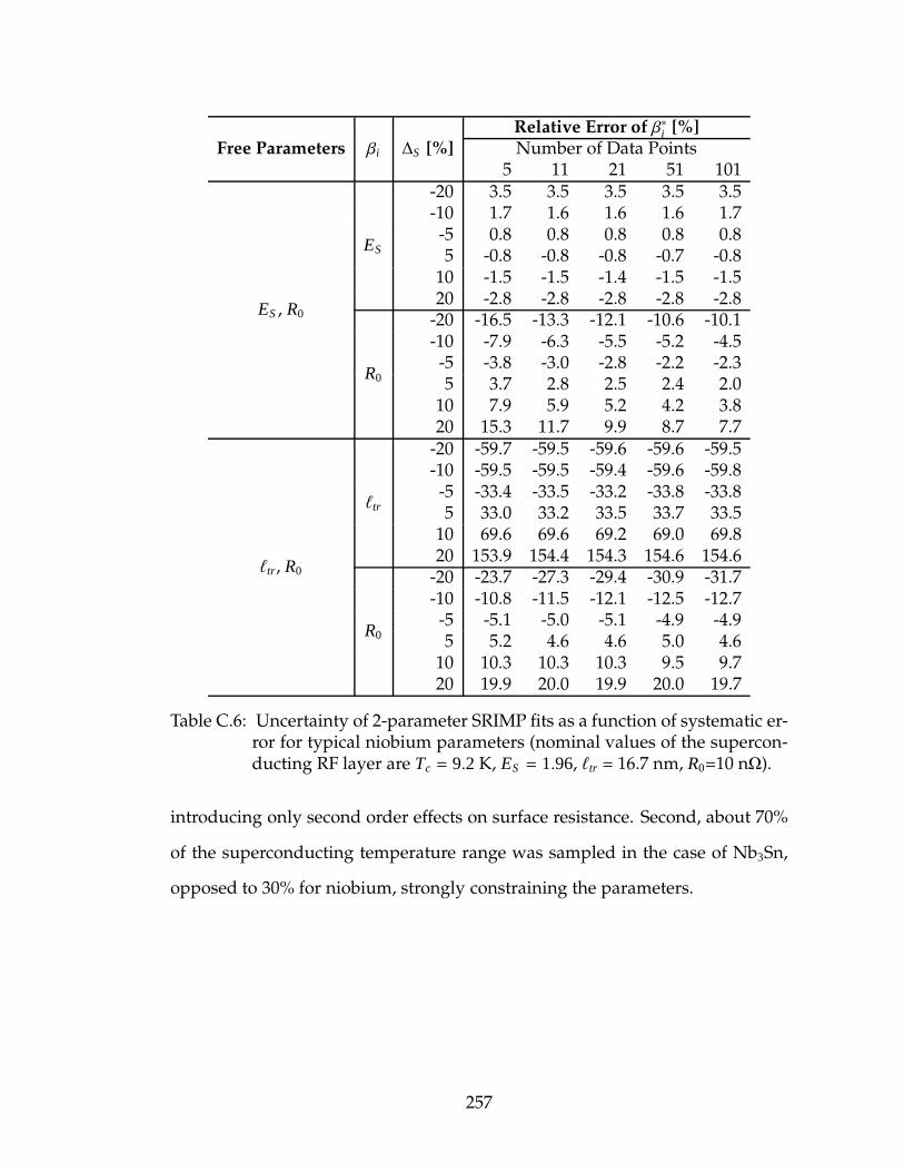
Free Parameters βi ∆S [%]Relative Error of β∗i [%]Number of Data Points
5 11 21 51 101
ES , R0
ES
-20 3.5 3.5 3.5 3.5 3.5-10 1.7 1.6 1.6 1.6 1.7
-5 0.8 0.8 0.8 0.8 0.85 -0.8 -0.8 -0.8 -0.7 -0.8
10 -1.5 -1.5 -1.4 -1.5 -1.520 -2.8 -2.8 -2.8 -2.8 -2.8
R0
-20 -16.5 -13.3 -12.1 -10.6 -10.1-10 -7.9 -6.3 -5.5 -5.2 -4.5
-5 -3.8 -3.0 -2.8 -2.2 -2.35 3.7 2.8 2.5 2.4 2.0
10 7.9 5.9 5.2 4.2 3.820 15.3 11.7 9.9 8.7 7.7
ℓtr, R0
ℓtr
-20 -59.7 -59.5 -59.6 -59.6 -59.5-10 -59.5 -59.5 -59.4 -59.6 -59.8
-5 -33.4 -33.5 -33.2 -33.8 -33.85 33.0 33.2 33.5 33.7 33.5
10 69.6 69.6 69.2 69.0 69.820 153.9 154.4 154.3 154.6 154.6
R0
-20 -23.7 -27.3 -29.4 -30.9 -31.7-10 -10.8 -11.5 -12.1 -12.5 -12.7
-5 -5.1 -5.0 -5.1 -4.9 -4.95 5.2 4.6 4.6 5.0 4.6
10 10.3 10.3 10.3 9.5 9.720 19.9 20.0 19.9 20.0 19.7
Table C.6: Uncertainty of 2-parameter SRIMP fits as a function of systematic er-ror for typical niobium parameters (nominal values of the supercon-ducting RF layer are Tc = 9.2 K, ES = 1.96, ℓtr = 16.7 nm, R0=10 nΩ).
introducing only second order effects on surface resistance. Second, about 70%
of the superconducting temperature range was sampled in the case of Nb3Sn,
opposed to 30% for niobium, strongly constraining the parameters.
257

Parameter Value Unit
Tc 18.0 KES 2.45 -λL 88.5 nmξS 11.0 nmℓtr 3.79 nmR0 9.365 nΩ
Table C.7: Nb3Sn material parameters used in Monte Carlo SRIMP fitting. [Pos]
258

2.2 2.4 2.6
5poin
ts5%
2.2 2.4 2.6
10%
2.2 2.4 2.6
20%
2.2 2.4 2.6
11
poin
ts
2.2 2.4 2.6 2.2 2.4 2.6
2.2 2.4 2.6
21
poin
ts
2.2 2.4 2.6 2.2 2.4 2.6
2.2 2.4 2.6
51
poin
ts
2.2 2.4 2.6 2.2 2.4 2.6
2.2 2.4 2.6
101
poin
ts
2.2 2.4 2.6
β ∈ [ES , ℓtr,R0], β∗i = ES
2.2 2.4 2.6
Figure C.13: Histograms showing the distribution of ES in 324 Monte Carlo sim-ulations of nominal Nb3Sn for various relative noise levels andnumber of data points in the measurement. The red curve is thebest fitting normal distribution, and the green line shows the nom-inal value of ES .
259
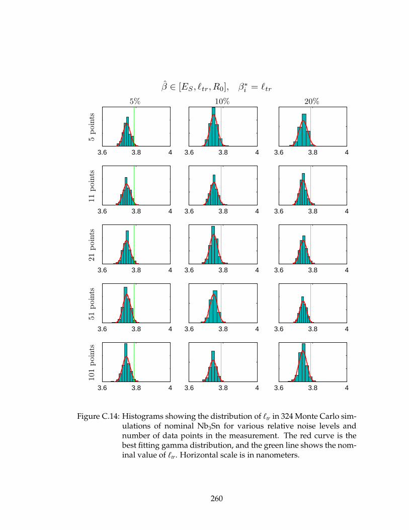
3.6 3.8 4
5poin
ts5%
3.6 3.8 4
10%
3.6 3.8 4
20%
3.6 3.8 4
11
poin
ts
3.6 3.8 4 3.6 3.8 4
3.6 3.8 4
21
poin
ts
3.6 3.8 4 3.6 3.8 4
3.6 3.8 4
51
poin
ts
3.6 3.8 4 3.6 3.8 4
3.6 3.8 4
101
poin
ts
3.6 3.8 4
β ∈ [ES , ℓtr,R0], β∗i = ℓtr
3.6 3.8 4
Figure C.14: Histograms showing the distribution of ℓtr in 324 Monte Carlo sim-ulations of nominal Nb3Sn for various relative noise levels andnumber of data points in the measurement. The red curve is thebest fitting gamma distribution, and the green line shows the nom-inal value of ℓtr. Horizontal scale is in nanometers.
260
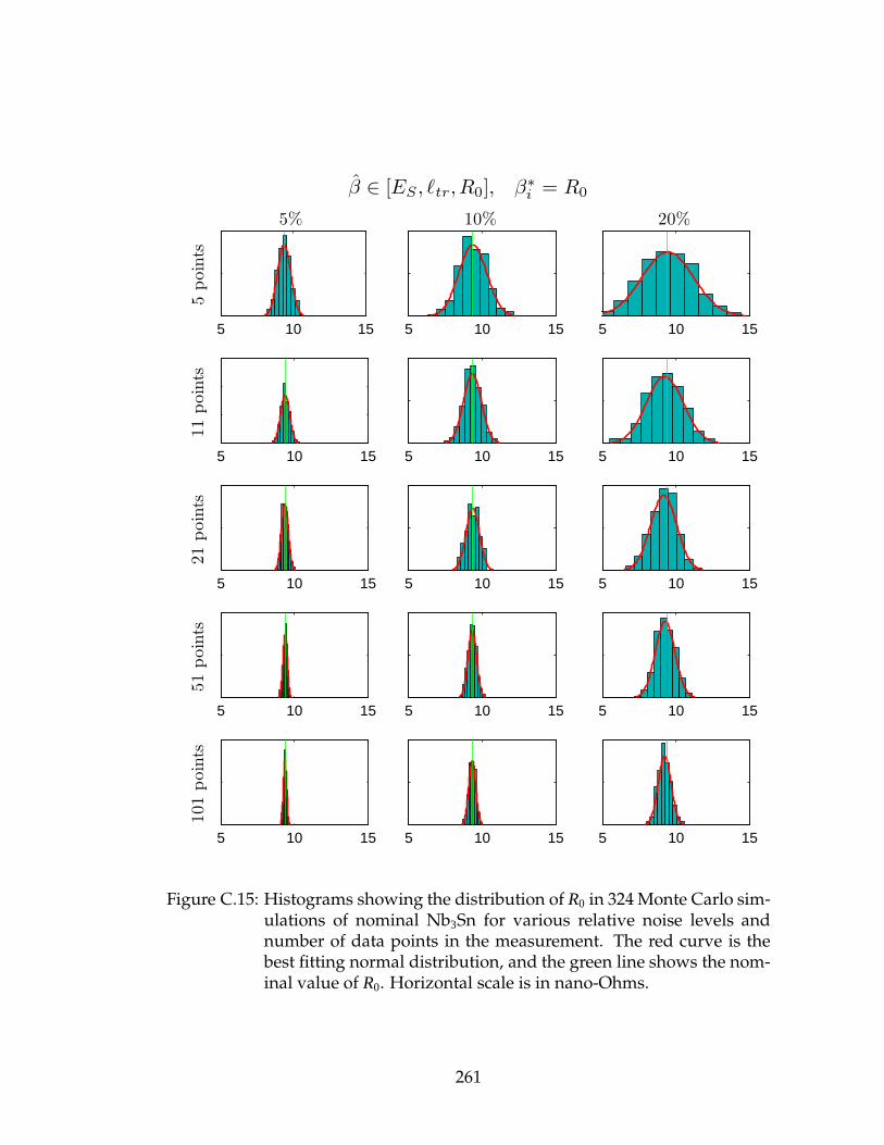
5 10 15
5poin
ts5%
5 10 15
10%
5 10 15
20%
5 10 15
11
poin
ts
5 10 15 5 10 15
5 10 15
21
poin
ts
5 10 15 5 10 15
5 10 15
51
poin
ts
5 10 15 5 10 15
5 10 15
101
poin
ts
5 10 15
β ∈ [ES , ℓtr,R0], β∗i = R0
5 10 15
Figure C.15: Histograms showing the distribution of R0 in 324 Monte Carlo sim-ulations of nominal Nb3Sn for various relative noise levels andnumber of data points in the measurement. The red curve is thebest fitting normal distribution, and the green line shows the nom-inal value of R0. Horizontal scale is in nano-Ohms.
261
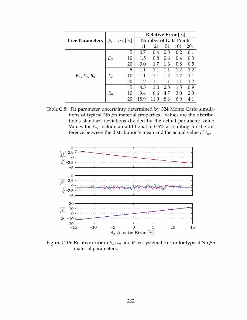
Free Parameters βi σR [%]Relative Error [%]
Number of Data Points11 21 51 101 201
ES , ℓtr, R0
ES
5 0.7 0.4 0.3 0.2 0.110 1.5 0.8 0.6 0.4 0.320 3.0 1.7 1.3 0.8 0.5
ℓtr
5 1.1 1.1 1.1 1.2 1.210 1.1 1.1 1.2 1.2 1.120 1.2 1.1 1.1 1.1 1.2
R0
5 4.5 3.0 2.3 1.5 0.910 9.4 6.6 4.7 3.0 2.320 18.9 11.9 8.6 6.9 4.1
Table C.8: Fit parameter uncertainty determined by 324 Monte Carlo simula-tions of typical Nb3Sn material properties. Values are the distribu-tion’s standard deviations divided by the actual parameter value.Values for ℓtr, include an additional ≈ 0.5% accounting for the dif-ference between the distribution’s mean and the actual value of ℓtr.
−5−2.5
02.5
5
ES
[%]
−5−2.5
02.5
5
ℓ tr
[%]
−15 −10 −5 0 5 10 15−20−10
01020
R0
[%]
Systematic Error [%]
Figure C.16: Relative error in ES , ℓtr and R0 vs systematic error for typical Nb3Snmaterial parameters.
262

C.4 Multiple Region Fitting
Section C.3 demonstrated that there is sloppiness in Tc and ES when fitting Rs
vs temperature data. It is possible, however, to gain confidence in Tc by fit-
ting penetration depth, λ(T ), as function of temperature. This either reduce the
number of free parameters in the model or give more confidence in determin-
ing Tc, and leads to lower uncertainties in the remaining parameters. From the
two-fluid model, [Bar58] one can approximate the temperature dependent pen-
etration depth as
λ(T ) = λL
√√√√ 1+ ξ
ℓ
1−(
TTc
)4− λ(T0) (C.11)
where ξ is the coherence length taking into account the electronic mean free
path ℓ, and λ(T0) is a fit parameter that sets the penetration depth at a given
temperature T0 (usually around 6-7 K). [Cio05]
The λ(T ) vs T measurement is performed by tracking the resonant frequency,
f (T ), of the cavity at a range of temperatures–preferably close to Tc. The pene-
tration depth is then given by the relation
λ(T ) − λ(T0) =1β
[
f (T ) − f (T0)]
, (C.12)
where β is a constant dependent on the geometry of the cavity. [Hal70a] Liepe
gives the value for the proportionality constant as
β =πµ0 f (T0)2
2G, (C.13)
where G is the geometry factor of the cavity and µ0 is the permeability of
free space. [Lie01] For the ERL 7-cell cavity, with G = 270 Ω, typically β ≈
12.4 kHz/µm. [She, GL13]
263

Because λ(T ) is sensitive to the critical temperature, it can be measured ac-
curately by noting the frequency shift near Tc. When data is available, it can
be used in combination with Rs data to determine a material’s SRF parameters
more accurately. This is carried out by applying the algorithm in section C.2
twice–once for Rs and once for λ(T )–and finding parameters that minimize the
weighted sum of both fit’s χ2. The algorithm performing the simultaneous op-
timization is presented below.
1 func t ion s o l a r r a y = . . .2 optimize rs and xd ( param array , da t rs , dat xd , varargin )3
4 Tc = param array 1 , 2 ;5 EnGap = param array 2 , 2 ;6 lonDepth = param array 3 , 2 ;7 cohLength= param array 4 , 2 ;8 RRR = param array 5 , 2 ;9 R0 = param array 6 , 2 ;
10 lambda 0 = param array 7 , 2 ;11
12 % Default weights13 weight . RS = 1 ;14 weight .XD = 1 ;15
16 i f ˜ isempty ( varargin ) && s i z e ( varargin , 2 ) ==217 weight . RS = varargin 1 ;18 weight .XD = varargin 2 ;19 end20
21 % Run an opt imiz a t ion22 guess = [ EnGap ; RRR ; R0 ; lambda 0 ] ;23 [ r e s u l t s , f i n a l R S S ] = fminsearch ( @compute rss , guess ) ;24
25 % Put the r e s u l t s i n t o a s o l u t i o n array26 s o l a r r a y = param array ;27 s o l a r r a y 2 ,2 = r e s u l t s ( 1 ) ;28 s o l a r r a y 5 ,2 = r e s u l t s ( 2 ) ;29 s o l a r r a y 6 ,2 = r e s u l t s ( 3 ) ;30 s o l a r r a y 7 ,2 = r e s u l t s ( 4 ) ;31 s o l a r r a y 8 ,3 = f i n a l R S S ;32
33 func t ion r s s = compute rss ( x )34 p array = . . .35 ’ Tc ’ , Tc , ’ f i x ’ ;36 ’EnGap ’ , x ( 1 ) , ’ f i x ’ ;37 ’ lonDepth ’ , lonDepth , ’ f i x ’ ;38 ’ cohLength ’ , cohLength , ’ f i x ’ ;39 ’RRR ’ , x ( 2 ) , ’ f i x ’ ;
264

40 ’R0 ’ , x ( 3 ) , ’ f i x ’ ;41 ’ Lambda 0 ’ , x ( 4 ) , ’ f i x ’ ;42 ;43
44 sol RS = polymorphic BCS f i t ( da t rs , p array , ’RS ’ ) ;45 sol XD = polymorphic BCS f i t ( dat xd , p array , ’XD ’ ) ;46
47 % Compute a weighting of the two RSS ’ s . ( Minimize t h i s )48 r s s = sol RS 8 ,3∗weight . RS + sol XD 8 ,3∗weight .XD;49 end50 end
In addition to allowing Tc to be determined accurately, fitting penetration
depth near Tc also has been used to determine ℓtr more accurately than with
surface resistance data alone. [GL13, GLG13]
C.5 Conclusion
A superconductor’s parameters can be extracted from either Rs vs temperature
or λ(T ) vs temperature data using the fitting algorithms discussed in this ap-
pendix. The statistically predicted confidence intervals are too small to include
the actual values used to generate validation data. To obtain more accurate con-
fidence intervals, Monte Carlo simulations were performed, and it was demon-
strated that for typical measurements (11–51 data points, taken between 1.4 and
4.2 K, with approximately 10% systematic error and 10% random error), the
relative uncertainty of the estimated parameters are less than 20%, with the ex-
ception of ℓtr which can have uncertainty of over 80%.
When fitting Tc, ES , ℓtr and R0, at the same time, the electronic mean free
path tends to be obtained with poor accuracy. This method should not be used
except for cases when there is no prior knowledge of the SRF parameters of the
265

material, which is seldom the case.
For niobium, more precise results are obtained by only fitting two param-
eters at a time. Whenever possible, as broad a temperature range as possible
should be used. Even greater precision is achievable when both penetration
depth data and surface resistance are fit simultaneously.
266
BIBLIOGRAPHY
[Aad12] Aad, G et al. Observation of a new particle in the search for thestandard model Higgs boson with the ATLAS detector at the LHC.Physics Letters B, 716(1):1 – 29, 2012.
[ABB+00] B. Aune, R. Bandelmann, D. Bloess, B. Bonin, A. Bosotti, M. Cham-pion, C. Crawford, G. Deppe, B. Dwersteg, D. A. Edwards, H. T.Edwards, M. Ferrario, M. Fouaidy, P.-D. Gall, A. Gamp, A. Gossel,J. Graber, D. Hubert, M. Huning, M. Juillard, T. Junquera,H. Kaiser, G. Kreps, M. Kuchnir, R. Lange, M. Leenen, M. Liepe,L. Lilje, A. Matheisen, W.-D. Moller, A. Mosnier, H. Padamsee,C. Pagani, M. Pekeler, H.-B. Peters, O. Peters, D. Proch, K. Rehlich,D. Reschke, H. Safa, T. Schilcher, P. Schmuser, J. Sekutowicz,S. Simrock, W. Singer, M. Tigner, D. Trines, K. Twarowski, G. We-ichert, J. Weisend, J. Wojtkiewicz, S. Wolff, and K. Zapfe. Super-conducting tesla cavities. Phys. Rev. ST Accel. Beams, 3:092001, Sep2000.
[Abr70] Milton Abramowitz. Handbook of mathematical functions : with for-mulas, graphs, and mathematical tables. Dover Publications, NewYork, 1970.
[Adm13] U.S. Energy Information Administration. Elec-tric power annual 2011. Online, January 2013.http://www.eia.gov/electricity/annual/pdf/epa.pdf.
[Age99] OECD Nuclear Energy Agency. Utilisation and Reliability of HighPower Proton Accelerators Workshop Proceedings, Aix-en-Provence,France, 22-24 November 1999. OECD Publishing, Paris, November1999.
[AKK12] S. Aull, O. Kugeler, and J. Knobloch. Trapped magnetic flux insuperconducting niobium samples. Phys. Rev. ST Accel. Beams,15:062001, Jun 2012.
[Ash76] Neil Ashcroft. Solid state physics. Holt, Rinehart and Winston, NewYork, 1976.
[Aue96] Pertti Auerkari. Mechanical and physical properties of engineering alu-mina ceramics. VTT Technical Research Center of Finland, 1996.
267
[Bab01] N. Baboi. Studies on higher order modes in accelerating structuresfor linear colliders. PhD thesis, Deutsches Elektronen-SynchrotronDESY, 2001.
[Bah98] Marko Bahte. Materialuntersuchungen an supraleitenden Niob-Probenmit Magnetisierungs- und Suszeptibilitatsmessungen. PhD thesis,Universitat Hamburg, March 1998.
[Bar58] John Bardeen. Two-fluid model of superconductivity. Phys. Rev.Lett., 1:399–400, Dec 1958.
[BBB+11] I. V. Bazarov, S. A. Belomestnykh, D. H. Bilderback, M. G. Billing,J. D. Brock, B. W. Buckley, S. S. Chapman, E. P. Chojnacki, Z. A.Conway, J. A. Crittenden, D. Dale, J. A. Dobbins, B. M. Dun-ham, R. D. Ehrlich, M. P. Ehrlichman, K. D. Finkelstein, E. Fontes,M. J. Forster, S. W. Gray, S. Greenwald, S. M. Gruner, C. Gulli-ford, D. L. Hartill, R. G. Helmke, G. H. Hoffstaetter, A. Kazimirov,R. P. Kaplan, S. S. Karkare, V. O. Kostroun, F. A. Laham, Y. H. Lau,Y. Li, X. Liu, M. U. Liepe, F. Loehl, L. Cultrera, C. E. Mayes, J. M.Maxson, A. Meseck, A. A. Mikhailichenko, D. Ouzounov, H. S.Padamsee, S. B. Peck, M. A. Pfeifer, S. E. Posen, K. W. Smolenski,P. G. Quigley, P. Revesz, D. H. Rice, U. Sae-Ueng, D. C. Sagan, J. O.Sears, V. D. Shemelin, C. K. Sinclair, D. M. Smilgies, E. N. Smith,C. Spethmann, C. Song, T. Tanabe, A. B. Temnykh, M. Tigner,N. R. A. Valles, V. G. Veshcherevich, Z. Wang, A. R. Woll, Y. Xie,and Z. Zhao. Cornell Energy Recovery Linac Project DefinitionDesign Report. Technical report, Cornell University, Mar 2011.
[BBD+10] Donald H Bilderback, Joel D Brock, Darren S Dale, Kenneth DFinkelstein, Mark A Pfeifer, and Sol M Gruner. Energy recov-ery linac (erl) coherent hard x-ray sources. New Journal of Physics,12(3):035011, 2010.
[BBD+12] S. Baradaran, U. Bergmann, H. Durr, K. Gaffney, J. Goldstein,M. Geuhr, J. Hastings, P. Heimann, R. Lee, and M. Seibert. LCLS-IInew instruments workshops report. Technical report, SLAC Na-tional Accelerator Laboratory, 2012.
[BCH+99] D. Boussard, E. Chiaveri, E. Haebel, H.P. Kindermann, R. Losito,S. Marque, V. Rodel, and M. Stirbet. The LHC superconductingcavities. In Proceedings of the 1999 Particle Accelerator Conference,1999.
268
[BCS57] J. Bardeen, L. N. Cooper, and J. R. Schrieffer. Microscopic Theoryof Superconductivity. Physical Review, 106:162–164, April 1957.
[BGK59] P. A. Bezuglyi, A. A. Galkin, and A. P. Korolyuk. Anisotropy of theabsorption coefficients of ultrasonics in superconductors. SOVIETPHYSICS JETP-USSR, 9(6):1388–1389, 1959.
[BH04] I. V. Bazarov and G. Hoffstaetter. Multi-pass beam-breakup: The-ory and calculation. In Proceedings of EPAC04, Lucerne/CH, 2004.
[BH07] Brandon Buckley and Georg H. Hoffstaetter. Transverse emittancedilution due to coupler kicks in linear accelerators. Phys. Rev. STAccel. Beams, 10:111002, Nov 2007.
[BHC+04] K. S. Brown, C. C. Hill, G. A. Calero, C. R. Myers, K. H. Lee, J. P.Sethna, and R. A. Cerione. The statistical mechanics of complexsignaling networks: nerve growth factor signaling. Physical Biol-ogy, 1(3):184, 2004.
[BLP+01] S. L. Bud’ko, G. Lapertot, C. Petrovic, C. E. Cunningham, N. An-derson, and P. C. Canfield. Boron isotope effect in superconduct-ing MgB2. Phys. Rev. Lett., 86:1877–1880, Feb 2001.
[Bra95] E. H. Brandt. The flux-line lattice in superconductors. Reports onProgress in Physics, 58(11):1465, 1995.
[Bro61] R. F. Broom. An Upper limit for the Resistivity of a Superconduct-ing Film. Nature, 190:992–993, June 1961.
[BS05] Egor Babaev and Martin Speight. Semi-Meissner state and neitherType-I nor Type-II superconductivity in multicomponent super-conductors. Phys. Rev. B, 72:180502, Nov 2005.
[CA99] E. Chojnacki and W. J. Alton. Beamline RF load development atCornell. In Proceedings of the 1999 Particle Accelerator Conference,volume 2, pages 845–847. IEEE, 1999.
[Cam87] Isodoro E. Campisi. On the Limiting RF Fields in SuperconductingAccelerator Cavities. SLAC AP-58, 1987.
[Car11] P. Carriere. Operating notes for BCP of dumbbells. CLASSE Notes,2011.
269

[CBJP11] C Cooper, B Bullock, S Joshi, and A Palczewski. Centrifugal barrelpolishing of cavities worldwide. In 15th International Conference onRF Superconductivity, Chicago, IL, 2011.
[CF84] I. E. Campisi and Z. D. Farkas. High-Gradient, Pulsed Operationof Superconducting Niobium Cavities. SLAC AP-16, 1984.
[Cha99] Alex Chao. Handbook of accelerator physics and engineering. WorldScientific, Singapore River Edge, N.J, 1999.
[Chi94] Yong Ho Chin. User’s guide for ABCI version 8.7 (Azimuthalbeam cavity interaction). 1994.
[Cho09] E. Chojnacki. Personal Communication, 2009.
[Cho10] E. Chojnacki. RF absorber studies at Cornell, including DC con-ductivity, part 2. Proceedings of 2010 Higher-Order Mode Work-shop, Oct 2010.
[CHPS09] Z. A. Conway, D. H. Hartill, H. Padamsee, and E. N. Smith. De-fect Location in Superconducting Cavities Cooled with He-II Us-ing Oscillating Superleak Transducers. In Proceedings of the 2009Particle Accelerator Conference, 2009.
[Cio05] G. Ciovati. Investigation of the superconducting properties of nio-bium radio-frequency cavities. PhD thesis, Old Dominion University,2005.
[Cio07] G. Ciovati. Review of high field Q-slope, cavity measurements. In13th International Workshop on RF Superconductivity, 2007.
[CKK+05] S. Casalbuoni, E.A. Knabbe, J. Ktzler, L. Lilje, L. von Sawilski,P. Schmser, and B. Steffen. Surface superconductivity in niobiumfor superconducting RF cavities. Nuclear Instruments and Meth-ods in Physics Research Section A: Accelerators, Spectrometers, Detec-tors and Associated Equipment, 538(13):45 – 64, 2005.
[Coo56] L. N. Cooper. Bound Electron Pairs in a Degenerate Fermi Gas.Physical Review, 104:1189–1190, November 1956.
[Coo06] CoorsTek Inc. CoorsTek Silicon Carbide: Material Properties, 2006.
270
[Cra46] Harald Cramer. Mathematical methods of statistics. Princeton Uni-versity Press, Princeton, 1946.
[CS08] G. Catelani and James P. Sethna. Temperature dependence of thesuperheating field for superconductors in the high-κ london limit.Phys. Rev. B, 78:224509, Dec 2008.
[DB98] R. J. Donnelly and C. F. Barenghi. The Observed Properties ofLiquid Helium at the Saturated Vapor Pressure. Journal of Physicaland Chemical Reference Data, 27:1217–1274, November 1998.
[DDBD96] Andrew J. Dolgert, S. John Di Bartolo, and Alan T. Dorsey. Super-heating fields of superconductors: Asymptotic analysis and nu-merical results. Phys. Rev. B, 53:5650–5660, Mar 1996.
[DEG+94] S. Doebert, R. Eichhorn, H. Genz, H.-D. Graef, R. Hahn, T. Ham-pel, J. Horn, C. Luettge, H. Loos, K. Ruehl, M. Reichenbach,A. Richter, P. Schardt, V. Schlott, G. Schrieder, E. Spamer,A. Stascheck, A. Stiller, M. Thomas, O. Titze, T. Wesp, andM. Wiencken. Status of the S-DALINAC and experimental de-velopments. In The Fourth European Particle Accelerator Conference,1994.
[DEM+87] B. Dwersteg, W. Ebeling, W.-D. Moller, D. Renken, D. Proch,J. Sekutowicz, J. Susta, and D. Tong. Superconducting cavities forHERA. In Proceedings of The Third Workshop on RF Superconductiv-ity, 1987.
[DeS63] Warren DeSorbo. Effect of dissolved gases on some superconduct-ing properties of niobium. Phys. Rev., 132(1):107–121, Oct 1963.
[dG65] P. G. de Gennes. Vortex nucleation in type II superconductors.Solid State Communications, 3(6):127 – 130, 1965.
[DG67] R. Doll and P. Graf. Superheating in cylinders of pure supercon-ducting tin. Phys. Rev. Lett., 19(16):897–899, Oct 1967.
[DGB+11] D. Dale, S. M. Gruner, J. Brock, D. Bilderback, and E. Fontes. Sci-ence at the hard x-ray diffraction limit (xdl2011), part 1. Syn-chrotron Radiation News, 24(6):4–11, 2011.
[DIPK91] M. Dzenus, K. Iversen, M. Peiniger, and D. Kiehlmann. Produc-
271
tion of superconducting niobium cavities for cebaf. In Proceedingsof the 1991 Particle Accelerator Conference, pages 2390–2392 vol.4,1991.
[DKM01] B. Dwersteg, D. Kostin, and W. D. Moeller. TESLA RF power cou-plers development at DESY. In Proc. of the 10th Workshop on RFSuperconductivity, Tsukuba, Japan, 2001.
[DMM+95] D. Dwersteg, A. Matheisen, W. D. Moller, D. Proch, D. Renken,and J. Sekutowicz. Operating experience with superconductingcavities in the HERA e-ring. In Proceedings of the 1995 Workshop onRF Superconductivity, 1995.
[EB64] F. Englert and R. Brout. Broken symmetry and the mass of gaugevector mesons. Phys. Rev. Lett., 13:321–323, Aug 1964.
[ECC97] Pascal Elleaume, Oleg Chubar, and Joel Chavanne. Computing 3Dmagnetic fields from insertion devices. In Proceedings of the 1997Particle Accelerator Conference, volume 3, pages 3509–3511. IEEE,1997.
[ECH+13] R. Eichhorn, J. Conway, Y. He, G. Hoffstaetter, Y. Li, M. Liepe,T. O’Connell, P. Quigley, J. Sears, V.D. Shemelin, and N. Valles.Cornell’s HOM beamline absorbers. In Proceedings of IPAC 2013,2013.
[Eds12] Alexander Edstrom. Non-pairwise vortex interactions inginzburg-landau theory of superconductivity. Master’s thesis,KTH, 2012.
[Eil68] G. Eilenberger. Transformation of Gorkov’s equation for typeII superconductors into transport-like equations. Zeitschrift furPhysik, 214(2):195–213, 1968.
[Eis54] Julian Eisenstein. Superconducting elements. Rev. Mod. Phys.,26:277–291, Jul 1954.
[Emm09] Paul Emma. First lasing of the LCLS X-ray FEL at 1.5 A. Proceed-ings of PAC09, 2009.
[EP06] G. Eremeev and H. Padamsee. Change in high field Q-slope bybaking and anodizing. Physica C: Superconductivity, 441(12):62 –
272
65, 2006. Proceedings of the 12th International Workshop on RFSuperconductivity.
[ES93] D. A. Edwards and M. J. Syphers. An introduction to the physics ofhigh energy accelerators. Wiley, New York, 1993.
[Far84] Z. D. Farkas. Low Loss Pulsed Mode Cavity Behavior. SLAC AP-15, 1984.
[Far98] S. Fartuokh. A new method to detect the high impedance modesof TESLA cavities. Technical report, CEA/DAPNIA/SEA, 1998.
[Fre68] R.A. French. Intrinsic type-2 superconductivity in pure niobium.Cryogenics, 8(5):301 – 308, 1968.
[FSS66] D. K. Finnemore, T. F. Stromberg, and C. A. Swenson. Supercon-ducting properties of high-purity niobium. Phys. Rev., 149(1):231–243, Sep 1966.
[GCPS05] R.L. Geng, C. Crawford, H. Padamsee, and A. Seaman. Verticalelectropolishing niobium cavities. In The 12th International Work-shop on RF Superconductivity, 2005.
[GE68] L. P. Gor’kov and G. M. Eliashberg. Generalization of theGinzburg-Landau Equations for Non-stationary Problems in theCase of Alloys with Paramagnetic Impurities. Soviet Journal of Ex-perimental and Theoretical Physics, 27:328–+, August 1968.
[GEPS07] R. L. Geng, G. V. Eremeev, H. Padamsee, and V. D. Shemelin. Highgradient studies for ILC with single-cell re-entrant shape and el-liptical shape cavities made of fine-grain and large-grain niobium.In Proceedings of PAC07, 2007.
[GHK64] G. S. Guralnik, C. R. Hagen, and T. W. B. Kibble. Global conserva-tion laws and massless particles. Phys. Rev. Lett., 13:585–587, Nov1964.
[GI94] F.A. Graybill and H.K. Iyer. Regression analysis: concepts and appli-cations. An Alexander Kugushev book. Duxbury Press, 1994.
[GL50] V. L Ginsburg and L. Landau. Zh. Eksp. Teor. Fiz., 20, 1950.
273
[GL13] D. Gonnella and M. Liepe. High Q0 studies at Cornell. In Proceed-ings of the 16th conference on RF Superconductivity, 2013.
[GLG13] D. Gonnella, M. Liepe, and A. Grassellino. Performance of aFNAL treated superconducting niobium cavity at Cornell. In Pro-ceedings of the 16th conference on RF Superconductivity, 2013.
[Gol97] D. A. Goldberg. Understanding the mixing of higher-order modesof multiply resonant systems. Technical Report LBL Report-39618,Lawrence Berkeley National Laboratory, 1 Cyclotron Road, Berke-ley, California 94720, 1997.
[Gol13] Dan Goldman. Measuring HOM properties in the HTC using mul-tiple methods. August 2013.
[Gor59] L.P. Gor’kov. Microscopic derivation of the Ginzburg-Landauequations in the theory of superconductivity. SOVIET PHYSICSJETP-USSR, 9(6):1364–1367, 1959.
[GR03] E. L. Garwin and M. Rabinowitz. Resistivity Ratio of NiobiumSuperconducting Cavities. eprint arXiv:cond-mat/0308266, August2003.
[GVL12] D. Gonnella, N. Valles, and M. Liepe. Automated cavity test suitefor Cornell’s ERL program. In Proceedings of IPAC2012, pages2372–2374, 2012.
[HA63] J. L Harden and V. Arp. The lower critical field in the ginzburg-landau theory of superconductivity. Cryogenics, 3(2):105 – 108,1963.
[Hal79] E. H. Hall. On a new action of the magnet on electric currents.American Journal of Mathematics, 2(3):pp. 287–292, 1879.
[Hal70a] J. Halbritter. Change of eigenstate in a superconducting RF cavitydue to a nonlinear response. Journal of Applied Physics, 41(11):4581–4588, 1970.
[Hal70b] J. Halbritter. Fortran-program for the computation of the surfaceimpedance of superconductors. KAROLA - OA-Volltextserverdes Forschungszentrums Karlsruhe [http://opac.fzk.de:81/oai/oai-2.0.cmp.S] (Germany), 1970.
274
[Har13] Michael Hartl. The tau manifesto. Online:http://tauday.com/tau-manifesto.pdf, June 2013.
[Haz88] Michiel Hazewinkel. Encyclopaedia of mathematics : an updated andannotated translation of the Soviet Mathematical encyclopaedia. ReidelSold and distributed in the U.S.A. and Canada by Kluwer Aca-demic Publishers, Dordrecht Boston Norwell, MA, U.S.A, 1988.
[HB04] Georg H. Hoffstaetter and Ivan V. Bazarov. Beam-breakup insta-bility theory for energy recovery linacs. Phys. Rev. ST Accel. Beams,7:054401, May 2004.
[HBS07] Georg H. Hoffstaetter, Ivan V. Bazarov, and Changsheng Song. Re-circulating beam-breakup thresholds for polarized higher-ordermodes with optical coupling. Phys. Rev. ST Accel. Beams, 10:044401,Apr 2007.
[Hei99] Matthias Hein. High-temperature superconducting thin films at mi-crowave frequencies. Springer, Berlin New York, 1999.
[Hig64] Peter W. Higgs. Broken symmetries and the masses of gaugebosons. Phys. Rev. Lett., 13:508–509, Oct 1964.
[Hoc13] A Hocker. High Q0 preservation. In Tesla Technology Collaborationon CW SRF, 2013.
[HP95] T. Hays and H. S. Padamsee. Determining HRFc for Nb and Nb3Sn
through HPP and Transient Q Analysis. In 7th Workshop on RFSuperconductivity, 1995.
[HPR95] T. Hays, H. S. Padamsee, and R. W. Roth. Response of supercon-ducting cavities to high peak power. In Proceedings of the 1995 U.S.Particle Accelerator Conference, 1995.
[IBM] IBM Corporation. Parameter estimates and standard errors (non-linear regression algorithms). Online.
[Jac98] John D. Jackson. Classical Electrodynamics Third Edition. Wiley,third edition, August 1998.
[Kay93] Steven Kay. Fundamentals of statistical signal processing. Prentice-Hall PTR, Englewood Cliffs, N.J, 1993.
275
[KCG+10] Kwok K., Arno Candel, Lixin Ge, Andreas Kabel, Rich Lee, Zeng-hai Li, Cho Ng, Vineet Rawat, and Greg Schussman. Advances inparallel electromagnetic codes for accelerator science and devel-opment. Technical Report 14349, SLAC, 2010.
[KCG+12] M. P. Kelly, Z. A. Conway, S. M. Gerbick, M. Kedzie, T. C. Reid,R. C. Murphy, and P. N. Ostroumov. Cold testing of supercon-ducting 72 MHz cavities for ATLAS. In Proceedings of LINAC 2012,Tel-Aviv Israel, 2012.
[Kit63] Charles Kittel. Quantum theory of solids. Wiley, New York, 1963.
[Kit86] Charles Kittel. Introduction to Solid State Physics. Wiley, 1986.
[KK35] W.H. Keesom and A.P. Keesom. New measurements on the spe-cific heat of liquid helium. Physica, 2(112):557 – 572, 1935.
[KMC+05] P. Kneisel, G.R. Myneni, G. Ciovati, J. Sekutowicz, and T. Carneiro.Performance of large grain and single crystal niobium cavities. InProceedings of the 12th Workshop on RF Superconductivity, 2005.
[KNV+09] O. Kugeler, A. Neumann, S. Voronenko, W. Anders, J. Knobloch,M. Schuster, A. Frahm, S. Klauke, D. Pfluckhahn, and S. Rotter-dam. Manipulating the intrinsic quality factor by thermal cyclingand magnetic fields. In 14th International Conference on RF Super-conductivity, 2009.
[KP97] J. Knobloch and H. Padamsee. Flux trapping in niobium cavitiesduring breakdown events. In Proceedings of SRF 1997, 1997.
[KSS67] MM Karliner, VE Shapiro, and IA Shekhtman. Instability in thewalls of a cavity due to ponderomotive forces of the electromag-netic field. Sov. Phys. Tech. Phys, 11, 1967.
[Lak13] Lake Shore Cryotronics, Inc. Hall (magnetic) sensor speci-fications. Online, http://www.lakeshore.com/products/Hall-Magnetic-Sensors/Pages/Specifications.aspx, 2013.
[Lan65] L.D. Landau. Collected papers of L. D. Landau. page 546. Gordonand Breach, 1965.
[Lev44] K. Levenberg. A method for the solution of certain non-linear
276

problems in least squares. Quarterly of Applied Mathematics,2(2):164–168, July 1944.
[LF99] Pao Lu and Joseph P Foy. Calculation of first sound speed in liquidhelium. Chinese Physics Letters, 16(4):276, 1999.
[LFF47] C. T. Lane, Henry A. Fairbank, and William M. Fairbank. SecondSound in Liquid Helium II. Phys. Rev., 71:600–605, May 1947.
[Lie01] Matthias U. Liepe. Superconducting Multicell Cavities for Linear Col-liders. PhD thesis, Universitat Hamburg, October 2001.
[LK06] M. Liepe and J. Knobloch. Superconducting RF for energy-recovery linacs. Nuclear Instruments and Methods in Physics ResearchA, 557:354–369, February 2006.
[LL35] F. London and H. London. The electromagnetic equations of thesupraconductor. Proceedings of the Royal Society of London. Series A,Mathematical and Physical Sciences, 149(866):pp. 71–88, 1935.
[LLNK09] L. Lee, Z. Li, C. Ng, and K. Ko. Omega3P: A parallel finite-elementeigenmode analysis code for accelerator cavities. Technical ReportSLAC-PUB-13529, SLAC National Accelerator Laboratory, 2575Sand Hill Road, Menlo Park, CA 94025, February 2009.
[M+99] W. D. Moeller et al. High power coupler for the tesla test facility.In 9th Workshop on RF Superconductivity, page 577, 1999.
[May09] C. Mayes. Energy Recovery Linear Accelerator Lattice Design and Co-herent Synchrotron Radiation. PhD thesis, Cornell University, 2009.
[May11] C. Mayes. Personal Communication, 2011.
[MB57] R. W. Morse and H. V. Bohm. Superconducting energy gap fromultrasonic attenuation measurements. Phys. Rev., 108:1094–1096,Nov 1957.
[MCD+90] A. Mosnier, S. Chel, M. Desmons, B. Hervieu, M. Maurier,B. Phung Ngoc, and A. Veyssiere. MACSE superconducting cavityRF drive system. In Proceedings of EPAC 1990, 1990.
277
[MDK03] Lia Merminga, David R. Douglas, and Geoffrey A. Krafft. High-current energy-recovering electron linacs. Annual Review of Nu-clear and Particle Science, 53(1):387–429, 2003.
[Mer68] J. R. Merrill. Type II Superconductivity Experiment. American Jour-nal of Physics, 36:133–136, February 1968.
[MGC63] B. T. Matthias, T. H. Geballe, and V. B. Compton. Superconductiv-ity. Rev. Mod. Phys., 35:1–22, Jan 1963.
[Mil86] R.H. Miller. Comparison of standing-wave and traveling-wavestructures. In Linear accelerator conference, Stanford, CA, USA, June1986.
[Mit91] S. Mitsunobu. Superconducting RF activities at KEK. In Proceed-ings of SRF 1991, 1991.
[MK05] G. R. Myneni and P. Kneisel. Springback in deep drawn high pu-rity niobium for superconductor cavities. In Materials Science &Technology, 2005.
[MO33] W. Meissner and R. Ochsenfeld. Ein neuer effekt bei eintritt dersupraleitfhigkeit. Naturwissenschaften, 21(44):787–788, 1933.
[Mos89] A. Mosnier. Developments of HOM couplers for superconductingcavities. In 4th Workshop on RF Superconductivity, 1989.
[MS67] J. Matricon and D. Saint-James. Superheating fields in supercon-ductors. Physics Letters A, 24:241–242, February 1967.
[MS69] R. Meservey and B. B. Schwartz. Equilibrium properties: Compar-ison of experimental results with predictions of the BCS theory.In R. D. Parks, editor, Superconductivity, Volume 1, pages 117–191.Marcel Dekker, 1969.
[MT01] G Materlik and Th. (Editors) Tschentscher. Tesla technical designreport. part v. Technical report, 2001.
[MY99] D.G. Myakishev and V. P. Yakovlev. CLANS2 - a code for calcu-lation of multipole modes in axisymmetric cavities with absorberferrites. In Proceedings of PAC 1999, pages 2775–2777, 1999.
278
[Myn07] Ganapati Rao Myneni. Physical and mechanical properties of nio-bium for SRF science and technology. AIP Conference Proceedings,927(1):41–47, 2007.
[Nat] National Energy Research Scientific Computing Center (NERSC).Office of Science and U.S. Department of Energy. Contract No.DE-AC02-05CH11231.
[NM75] V. Novotny and P.P.M. Meincke. Single superconducting energygap in pure niobium. Journal of Low Temperature Physics, 18(1-2):147–157, 1975.
[Nob13a] Nobel Media AB. Heike Kamerlingh Onnes - Biographical. Web,September 2013.
[Nob13b] Nobel Media AB. The Nobel Prize in Physics 2013. Web, Novem-ber 2013.
[OMFB79] T. P. Orlando, E. J. McNiff, S. Foner, and M. R. Beasley. Criticalfields, pauli paramagnetic limiting, and material parameters ofNb3sn and V3Si. Phys. Rev. B, 19:4545–4561, May 1979.
[Onn] H. Kamerlingh Onnes. Research Notebooks 56, 57. KamerlinghOnnes Archive, Boerhaave Museum, Leiden, the Netherlands.
[Onn11] H. Kamerlingh Onnes. Further experiments with liquid helium. d.on the change of the electrical resistance of pure metals at very lowtemperatures, etc. v. the disappearance of the resistance of mer-cury. In Jonhannes Muller, editor, Royal Netherlands Academy ofArts and Sciences (KNAW), volume 14, pages 113–115, May 1911.
[OSB+12] J. F. Ostiguy, N. Solyak, P. Berrutti, J. P. Carneiro, V. Lebedev, S. Na-gaitsev, A. Saini, B. Stheynas, and V. P. Yakovlev. Status of theProject-X CW linac design. In Proceedings of IPAC 2012, 2012.
[PA98] Paul J. Petersan and Steven M. Anlage. Measurement of resonantfrequency and quality factor of microwave resonators: Compari-son of methods. Journal of Applied Physics, 84(6):3392–3402, 1998.
[Pad09] H. Padamsee. RF Superconductivity: Volume II: Science, Technologyand Applications. Rf Superconductivity. Wiley, 2009.
279
[Pal01] Robert Palais. π is wrong! The Mathematical Intelligencer, 23(3):7–8,2001.
[Pan05] High Energy Physics Advisory Panel. Discovering the quantumuniverse. Technical report, United States Department of Energyand the National Science Foundation, 2005.
[PCL+13] S. Posen, G. Catelani, M. U. Liepe, J. P. Sethna, and M. K.Transtrum. Theoretical Field Limits for Multi-Layer Superconduc-tors. ArXiv e-prints, September 2013.
[Per66] John M. Perz. Attenuation of ultrasonic waves of arbitrary polar-ization and propagation direction in superconductors. CanadianJournal of Physics, 44(8):1765–1779, 1966.
[Pip53] A. B. Pippard. An experimental and theoretical study of the re-lation between magnetic field and current in a superconductor.Proceedings of the Royal Society of London. Series A. Mathematical andPhysical Sciences, 216(1127):547–568, 1953.
[PKH98] H. Padamsee, J. Knobloch, and T. Hays. RF superconductivity foraccelerators. Wiley, New York, 1998.
[PL11] S. Posen and M. Liepe. Stochiometric nb3sn in first samples coatedat Cornell. In 15th International Conference on RF Superconductivity,2011.
[PL12a] S. Posen and M. Liepe. Measurement of the mechanical propertiesof superconducting cavities during operation. In Proceedings ofIPAC 2012, 2012.
[PL12b] S. Posen and M. Liepe. Mechanical designs of SRF cavities for cwoperation - d f /dp and stiffening rings theory and measurement.In Proceedings of IPAC 2012, 2012.
[PL12c] S. Posen and M. Liepe. Minimizing helium pressure sensitivity inelliptical srf cavities. In Proceedings of IPAC2012, 2012.
[Poo99] Charles P. Poole. Handbook of Superconductivity. Academic Press,1999.
[Pos] S. Posen. Personal Communication.
280
[Pos13a] S. Posen. First cavity results from the Cornell SRF group’s Nb3Snprogram. In Proceedings of NA-PAC 2013, 2013.
[Pos13b] S. Posen. SRF cavities beyond niobium: Potential and challenges.In Proceedings of NA-PAC 2013, 2013.
[Poz05] D.M. Pozar. Microwave Engineering. Wiley, third edition, 2005.
[PW56] W. K. H. Panofsky and W. A. Wenzel. Some Considerations Con-cerning the Transverse Deflection of Charged Particles in Radio-Frequency Fields. Review of Scientific Instruments, 27:967, Novem-ber 1956.
[RAB+95] T. Raubenheimer, C. Adolphsen, D. Burke, P. Chen, S. Ecklund,J. Irwin, G. Loew, T. Markiewicz, R. Miller, E. Paterson, N. Phin-ney, M. Ross, R. Ruth, J. Sheppard, H. Tang, K. Thompson, andP. Wilson. Parameters of the SLAC Next Linear Collider. In Par-ticle Accelerator Conference, 1995., Proceedings of the 1995, volume 2,pages 698–700 vol.2, 1995.
[RAG+11] D Reschke, S Aderhold, A Gossel, J Iversen, S Karstensen,D Kostin, G Kreps, A Matheisen, WD Moller, F Schlander, et al.Results on large grain nine-cell cavities at DESY: Gradients up to45 MV/m after electropolishing. In 15th International Conference onRF Superconductivity, pages 490–494, 2011.
[Rao09] Singiresu Rao. Engineering optimization theory and practice. JohnWiley & Sons, Hoboken, N.J, 2009.
[RGBO13] A. Romanenko, A. Grassellino, F. Barkov, and J. P. Ozelis. Effectof mild baking on superconducting niobium cavities investigatedby sequential nanoremoval. Phys. Rev. ST Accel. Beams, 16:012001,Jan 2013.
[ROGP12] A. Romanenko, J. P. Ozelis, A. Grassellino, and H. Padamsee.Depth distribution of losses in superconducting niobium cavities.In Proceedings of IPAC2012, 2012.
[Roh04] James William Rohlf. Modern physics from α to Z0. Wiley, 2004.
[RR67] J.C. Renard and Y.A. Rocher. Superheating in pure superconduct-ing niobium. Physics Letters A, 24(10):509 – 511, 1967.
281
[RS39] B.V. Rollin and F. Simon. On the ”film” phenomenon of liquidhelium II. Physica, 6(2):219 – 230, 1939.
[SAB+79] F. Steglich, J. Aarts, C. D. Bredl, W. Lieke, D. Meschede, W. Franz,and H. Schafer. Superconductivity in the presence of strong pauliparamagnetism: CeCu2Si2. Phys. Rev. Lett., 43:1892–1896, Dec1979.
[SAE+13] T. Saeki, Y. Ajima, K. Enami, H. Hayano, H. Inoue, E. Kako,S. Kato, S. Koike, T. Kubo, S. Noguchi, M. Satoh, M. Sawabe,T. Shishido, A. Terashima, N. Toge, K. Ueno, K. Umemori,K. Watanabe, Y. Watanabe, S. Yamaguchi, A. Yamamoto, Y. Ya-mamoto, M. Yamanaka, K. Yokoya, Y. Iwashita, F. Yasuda,N. Kawabata, H. Nakamura, K. Nohara, and M. Shinohara. Studyon fabrication of superconducting RF 9-cell cavity for ILC at KEK.In Proceedings of the 2013 International Particle Accelerator Confer-ence, 2013.
[Sag06] D. Sagan. Bmad: A relativistic charged particle simulation library.Nuclear Instruments and Methods in Physics Research A, 558:356–359,March 2006.
[SB10] V. Shemelin and S. Belomestnykh. Using a resistive material forHOM damping. In Proceedings of IPAC 2010, 2010.
[SBC70] F.W. Smith, A. Baratoff, and M. Cardona. Superheating, super-cooling, surface superconductivity and ginzburg-landau param-eters of pure type-i superconductors and their alloys. Physik derkondensierten Materie, 12(2):145–192, 1970.
[SBG+03] V. Shemelin, S. Belomestnykh, R. L. Geng, M. Liepe, andH. Padamsee. Dipole-mode free and kick-free 2-cell cavity for theSC ERL injector. In Proceedings of PAC 2003, 2003.
[SC12] V. Shemelin and P. Carriere. Frequency control in the process ofa multicell superconducting cavity production. Review of ScientificInstruments, 83(4):043304, 2012.
[Sch92] P. Schmuser. Tuning of multi-cell cavities using bead pull mea-surements. Technical report, DESY, 1992. SRF920925-10.
[Sch11] M. Schuh. Study of Higher Order Modes in Superconducting Acceler-
282

ating Structures for Linac Applications. PhD thesis, Ruperto-CarolaUniversity of Heidelberg, Germany, June 2011.
[Sek12] J. K. Sekutowicz. Superconducting elliptical cavities. ArXiv e-prints, January 2012.
[SH06] Changsheng Song and Georg H Hoffstaetter. Lon-gitudinal bbu threshold current in recirculatinglinacs. Technical report, Cornell University, 2006.http://www.lepp.cornell.edu/∼hoff/hoff/papers/ERL06-04.pdf.
[SH07] Changsheng Song and Georg H Hoffstaetter. Trans-verse quadrupole bbu threshold current in the cornellx-ray erl. Technical report, Cornell University, 2007.http://www.lepp.cornell.edu/∼hoff/hoff/papers/ERL06-04.pdf.
[She] V. Shemelin. Personal Communication.
[She09a] V. Shemelin. Comparison of shape of multicell cavity cells. In 14thInternational Conference on RF Superconductivity, 2009.
[She09b] V. D. Shemelin. Suppression of HOMs in a multicell supercon-ducting cavity for Cornell’s ERL. In 14th International Conferenceon RF Superconductivity, 2009.
[She11] Valery Shemelin. Corrections of a superconducting cavity shapedue to etching, cooling down, and tuning. In 15th InternationalConference on RF Superconductivity, volume 10, page 1, 2011.
[Sin12] W. Singer. Superconducting 1.3 GHz Cavities for European XFEL.In The XXIII Russian Particle Accelerator Conference, 2012.
[SKG+05] Jacek Sekutowicz, K Ko, L Ge, L Lee, Zenghai Li, C Ng, G Schuss-man, Liling Xiao, I Gonin, T Khabibouline, et al. Design of a lowloss srf cavity for the ilc. In Particle Accelerator Conference, 2005.PAC 2005. Proceedings of the, pages 3342–3344. IEEE, 2005.
[Sla50] J. C. Slater. Microwave Electronics. D. Van Nostrand Company,Princeton, 1950.
[Sla97] J. P. H. Sladen. Status of superconducting cavities in lep. ParticleAccelerators, 60(CERN-SL-97-062-RF):15–25, 1997.
283
[SMZ89] M.C. Sanchez, E. Martin, and J.-M. Zamarro. New vectorial au-tomatic technique for characterisation of resonators. Microwaves,Antennas and Propagation, IEE Proceedings H, 136(2):147–150, 1989.
[Son98] Jeff E. Sonier. The Magnetic Penetration Depth and the Vortex CoreRadius in Type-II Superconductors. PhD thesis, University of BritishColumbia, April 1998.
[SR07] Tsun-Kong Sham and Richard A. Rosenberg. Time-resolved syn-chrotron radiation excited optical luminescence: Light-emissionproperties of silicon-based nanostructures. ChemPhysChem,8(18):2557–2567, 2007.
[STU08] STUDENT. The probable error of a mean. Biometrika, 6(1):1–25,1908.
[SW03] G.A.F. Seber and C.J. Wild. Nonlinear Regression. Wiley Series inProbability and Statistics. Wiley, 2003.
[TBD+05] C. D. Tennant, K. B. Beard, D. R. Douglas, K. C. Jordan, L. Mer-minga, E. G. Pozdeyev, and T. I. Smith. First observations andsuppression of multipass, multibunch beam breakup in the jeffer-son laboratory free electron laser upgrade. Phys. Rev. ST Accel.Beams, 8:074403, Jul 2005.
[TCS11] Mark K. Transtrum, Gianluigi Catelani, and James P. Sethna. Su-perheating field of superconductors within ginzburg-landau the-ory. Phys. Rev. B, 83:094505, Mar 2011.
[Tem08] Alexander B. Temnykh. Delta undulator for Cornell energy recov-ery linac. Phys. Rev. ST Accel. Beams, 11:120702, Dec 2008.
[Ten06] C. D. Tennant. Studies of Energy Recovery Linacs at Jefferson Labora-tory. PhD thesis, College of William and Mary, October 2006.
[TFT87] Yuzo Kojima Shinji Mitsunobu Hirotaka Nakai ToshiharuNakazato Shuichi Noguchi Kenji Saito Takaaki Furuya, Kiy-omitsu Asano and Tsuyoshi Tajima. The TRISTAN superconduct-ing cavities. In Proceedings of the Third Workshop on RF Supercon-ductivity, 1987.
[The13a] The International Linear Collider Collaboration. The International
284
Linear Collider Technical Design Report. Volume 3, Part II. Tech-nical report, 2013.
[The13b] The MathWorks, Inc., 3 Apple Hill Drive, Natick, Massachusetts01760 USA. MatLab Documentation Center: findpeaks, 2013.http://www.mathworks.com/help/signal/ref/findpeaks.html.
[Tig65] M. Tigner. A possible apparatus for electron clashing-beam exper-iments. Nuovo Cim., 37:1228–1231, 1965.
[Tin04] Michael Tinkham. Introduction to superconductivity. Dover Publi-cations, Mineola, N.Y, 2004.
[Tis38] L. Tisza. Transport Phenomena in Helium II. Nature, 141:913, May1938.
[TM80] A. A. Teplov and M. N. Mikheeva. Parallel critical magnetic fieldsfor superconducting vanadium and technetium films. Zh. Eksp.Teor. Fiz, 79:2302–2310, 1980.
[Tra11a] M. Transtrum. Personal Communication, 2011.
[Tra11b] M. Transtrum. Information Geometry for Nonlinear Least-SquaresData Fitting and Calculation of the Superconducting SuperheatingField. PhD thesis, Cornell University, 2011.
[Val12] N. Valles. High Q cavities at Cornell. In 7th SRF Materials Work-shop, 2012.
[VB09] V. Veshcherevich and S. Belomestnykh. Input coupler for mainlinac of Cornell ERL. In The 14th Internation Conference on RF Su-perconductivity, 2009.
[VBB+92] C Vallet, M Bolore, B Bonin, JP Charrier, B Daillant, J Gratadour,F Koechlin, and H Safa. Flux trapping in superconducting cavities.In Proc. of the European Particle Accelerator Conference EPAC92, page1295, 1992.
[VBLM12] N Valles, M. Billing, G. HofG. Hoffstaetter. Liepe, and C. Mayes.HOM studies of the cornell ERL prototype cavity in a horizontaltest cryomodule. In Proceedings of IPAC2012, 2012.
285
[VCL09] N. R. A. Valles, Z. A. Conway, and M. Liepe. Exploring the maxi-mum superheating fields of niobium. In 14th International Confer-ence on RF Superconductivity, 2009.
[vdHAP+07] B. van der Horst, A.Matheisen, B. Petersen, S. Saegebarth, andP. Schilling. Update on cavity preparation for high gradient su-perconducting multicell cavities at desy. In The 13th InternationalWorkshop on RF Superconductivity, 2007.
[VEF+13] N. Valles, R. Eichhorn, F. Furuta, M. Ge, D. Gonnella, Y. He,K. Ho, G. Hoffstaetter, M. Liepe, T. O’Connell, S. Posen, P. Quigley,J. Sears, and V. Veshcherevich. Cornell ERL main linac 7-cell cav-ity performance in horizontal test cryomodule qualifications. InProceedings of IPAC 2013. CLASSE, 2013.
[Ves] V. Veshcherevich. Personal Communication.
[VFG+12] N. Valles, F. Furuta, M. Ge, Y. He, K. M. V. Ho, G. H. Hoffstaetter,M. Liepe, T. O’Connell, S. Posen, P. Quigley, J. Sears, M. Tigner,and V. Veshcherevich. Testing of the main-linac prototype cavityin a horizontal test cryomodule for the Cornell ERL. In Proceedingsof IPAC 2012, 2012.
[VKK13] J. Vogt, O. Kugeler, and J. Knobloch. Studies of systematic fluxreduction in superconducting Nb. In Proceedings of IPAC 2013.Helmholtz-Zentrum fr Materialien und Energie (HZB), 2013.
[VKL11] N. Valles, D. S. Klien, and M. Liepe. Beam break-up studies forcornell’s energy recovery linac. In 15th International Conference onRF Superconductivity, 2011.
[VL09] N. Valles and M. Liepe. Seven-cell cavity optimization for Cor-nell’s energy recovery linac. In 14th International Conference on RFSuperconductivity, 2009.
[VL10a] N. Valles and M. Liepe. Baseline cavity design for Cornell’s energyrecovery linac. In International Particle Accelerator Conference, 2010.
[VL10b] N. Valles and M. Liepe. Cavity design for Cornell’s energy recov-ery linac. In Proceedings of IPAC 2010, 2010.
286
[VL11] N. Valles and M. Liepe. Designing multiple cavity classes for themain linac of Cornell’s ERL. In Proceedings of PAC 2011, 2011.
[VL12] N. Valles and M. Liepe. HOM studies on the Cornell ERL proto-type cavity in a horizontal test cryomodule. In Proceedings of IPAC2012, 2012.
[VLF+14] N. Valles, M. Liepe, F. Furuta, M. Gi, D. Gonnella, Y. He, K. Ho,G. Hoffstaetter, D.S. Klein, T. O’Connell, S. Posen, P. Quigley,J. Sears, G.Q. Stedman, M. Tigner, and V. Veshcherevich. Themain linac cavity for cornell’s energy recovery linac: Cavity de-sign through horizontal cryomodule prototype test. Nuclear In-struments and Methods in Physics Research Section A: Accelerators,Spectrometers, Detectors and Associated Equipment, 734, Part A(0):23– 31, 2014.
[VLS11] N. Valles, M. Liepe, and V. Shemelin. Coupler kick studies in Cor-nells 7-cell superconducting cavities. In 15th International Confer-ence on RF Superconductivity, Chicago, IL US, 2011.
[VSP05] M. Liepe V. Shemelin and H. Padamsee. Measurements of ǫ andµ of lossy materials for the cryogenic HOM load. In Proceedings ofPAC 2005, 2005.
[Wer69] N. R. Werthamer. The Ginzburg-Landau equations and their ex-tensions. In R. D. Parks, editor, Superconductivity, Volume 1, pages321–370. Marcel Dekker, 1969.
[Wie95] Helmut Wiedemann. Particle accelerator physics. Springer, Berlinu.a, 1995.
[Wil00] Klaus Wille. The physics of particle accelerators : an introduction. Ox-ford University Press, Oxford New York, 2000.
[Xia97] Z. Xiaowei. Parallel electromagnetic field solvers using finite elementmethods with adaptive refinement and their application to wakefieldcomputation of axisymmetric accelerator structure. PhD thesis, 1997.Copyright - Copyright UMI - Dissertations Publishing 1997; Lastupdated - 2010-08-07; First page - n/a; M3: Ph.D.
[XKL+11] L. Xiao, K. Ko, K. Lee, M. Liepe, and N. Valles. Effects of ellipti-cally deformed cell shape in the Cornell ERL cavity. In 15th Inter-national Conference on RF Superconductivity, 2011.
287

[Yak11] V. Yakolev. Transverse impedance definitions. Personal Commu-nication, 2011.
[YDM77] T. Yogi, G. J. Dick, and J. E. Mercereau. Critical rf Magnetic Fieldsfor Some Type-I and Type-II Superconductors. Phys. Rev. Lett.,39(13):826–829, Sep 1977.
288