Embed Size (px)
Citation preview
PSYCHOMETRIKA--VOL. 67, NO. 1, 79-94 MARCH 2002
STATISTICAL INFERENCE OF MINIMUM RANK FACTOR ANALYSIS
ALEXANDER SHAPIRO
SCHOOL OF INDUSTRIAL AND SYSTEMS ENGINEERING
GEORGIA INSTITUTE OF TECHNOLOGY
Jos M.F. TEN BERGE
HEYMANS INSTITUTE OF PSYCHOLOGICAL RESEARCH
UNIVERSITY OF GRONINGEN
For any given number of factors, Minimum Rank Factor Analysis yields optimal communalifies for an observed covaxiance matrix in the sense that the unexplained common variance with that number of factors is minimized, subject to the constraint that both the diagonal matrix of unique variances and the observed covariance matrix minus that diagonal matrix are positive semidefinite. As a result, it becomes possible to distinguish the explained common variance from the total common variance. The percentage of explained common variance is similar in meaning to the percentage of explained observed variance in Principal Component Analysis, but typically the former is much closer to 100 than the latter. So fax, no statistical theory of MRFA has been developed. The present paper is a first start. It yields closed-form ex- pressions for the asymptotic bias of the explained common variance, or, more precisely, of the unexplained common variance, under the assumption of multivariate normality. Also, the asymptotic variance of this bias is derived, and also the asymptotic covaxiance matrix of the unique variances that define a MRFA solution. The presented asymptotic statistical inference is based on a recently developed perturbation the- ory of semidefinite programming. A numerical example is also offered to demonstrate the accuracy of the expressions.
Key words: factor analysis, communalities, proper solutions, explained common variance, semidefinite programming, large samples asymptotics, asymptotic normality, asymptotic bias.
1. Introduction
Factor analysis is based on the notion that given a set of variables Zl . . . . . zp, each variable z j can be decomposed into a common part cj and a unique part u j , assumed to be uncorrelated with any variable except z j , j = 1 . . . . . p . Upon writing
z j = cj + u j , (1)
j = 1 . . . . . p, and using the assumption on u j , we have
= ]~c + air, (2)
where ~ is the covariance matrix of the variables, ~ is the diagonal matrix of unique variances, and £ c is the variance-covariance matrix of the common parts c j , j = 1 . . . . . p, of the vari- ables. The variances of these common parts are in the diagonal of ]~c. They are the so-called communalities of the variables.
The ideal of factor analysis is to find a decomposition (2) with £ c of low rank r, which can be factored as Zc = FF I, with F a p × r matrix. To accomplish this, communalities are required that reduce the rank of ~ - ~ to some small value. Although the early days of factor analysis were characterized by great optimism in this respect (Ledermann, 1937), the ideal of low reduced rank will never be attained in practice, see Guttman (1958) and Shapiro (1982). A
This work was supported, in part, by grant DMS-0073770 from the National Science Foundation. Requests for reprints should be sent to Alexander Shapiro, School of Industrial and Systems Engineering, Georgia
Institute of Technology, Atlanta, Georgia 30332-0205. E-Mail: [email protected]
0033-3123/2002-1/2000-0824-A $00.75/0 @ 2002 The Psychometric Society
79
80 PSYCHOMETRIKA
historical overview of how the ideal of low reduced rank was shattered can be found in ten Berge (1998).
For practical purposes, there is no choice other than trying to approximate the ideal low rank situation by using the eigendecomposition £c = £1 + £2, of the covariance matrix of the common parts, where both matrices £1 and £2 are positive semidefinite, matrix £1 has rank r (for some small value of r), and r nonzero eigenvalues of £1 coincide with r largest eigenvalues of ]~c. This leads to the following decomposition of 1~,
£ = FF' + (£c - FF') + Rt. (3)
This means that the variances of the variables (diagonal elements of ~) are decomposed into ex- plained common variances (diagonal elements of FF~), unexplained common variances (diagonal elements of £c - FF~), and unique variances (diagonal elements of Rt).
It is essential to note that a proper solution for (3) requires that both matrices £c and Rt should be positive semidefinite (denoted £c _> 0 and Rt _> 0, respectively). Negative elements in Rt, known as Heywood cases, have drawn a lot of attention, and are usually not tolerated. However, when £c, the covariance matrix for the common parts of the variables, would appear to be indefinite, that would be no less embarrassing than having a negative unique variance in Rt. Nevertheless, popular methods of common factor analysis generally ignore the constraint that £c - FF ~ must be positive semidefinite. The only exception seems to be Minimum Rank Fac- tor Analysis (MRFA). This method was originally proposed by ten Berge and Kiers (1991) as AMRFA, but the "A" of approximate has worn oft" in the meantime. MRFA offers a decomposi- tion of ~ that satisfies (3), with both Rt and £c - FF ~ positive semidefinite. Subject to these two constraints, MRFA constructs the solution that minimizes the unexplained common variance for anyfixed number offactors r. In other words, MRFA approximates the ideal of low reduced rank by minimizing the amount of common variance that is left unexplained when as few as r factors are maintained.
For a p x p symmetric matrix S we denote by )Vl (S) _> .. • _> )vp (S) its eigenvalues arranged in decreasing order. Formally, MRFA minimizes, for fixed r, the function
p
fmrfa(Rt) := Z )vi(£ - Rt) (4) i=r+l
subject to £ - a I t _> 0 and aI t _> O. This is very similar to MINRES/IPFA/ULS, where the function
p fmin~es0I') := ~ )'2(X -- 'I ') (5)
i=r+l
is minimized, without any constraint on the sign of these eigenvalues (Harman & Jones, 1966, JOreskog, 1967). A similar eigenvalue interpretation of Maximum Likelihood Factor Analysis has been given by JOreskog (1967, p. 449), also see ten Berge (1998) for a discussion.
A key feature of (3) is the distinction between communalities as variances "to be explained" on the one hand, and the explained variances of the variables, the diagonal elements of FF I on the other. The difference rests in the unexplained parts of the communalities, in the diagonal of £c - FF I. When this distinction is preserved, it is possible to evaluate to what extent the com- mon variance is accounted for by the common factors. This can be expressed as "the percentage of explained common variance", analogous to the percentage of explained observed variance in Principal Component Analysis. So far, MRFA is the only method that solves (3) subject to its constraints. Hence it is the only method so far that yields a percentage of explained common variance, to guide decisions about the number of factors to retain. Consider, for instance, the situation where only one common factor is hypothesized to account for the correlations between variables. MRFA will give the smallest possible percentage of common variance that is left unex-
ALEXANDER SHAPIRO AND JOS M.F. TEN BERGE 81
plained under the one-factor hypothesis. This means that MRFA evaluates the extent to which a one factor hypothesis is untenable, under the most favorable conditions for the that very hypoth- esis, namely, the MRFA communalit i tes with r = 1. The same logic applies to r hypothesized factors in general.
In practical applications, MRFA decomposes the sample analog of 1~. A key question, there- fore, is the extent to which the sample statistics in general, and the explained common variance in particular, are reliable. The present paper deals with the bias of the explained common vari- ance (ECV) with MRFA, or, more precisely, with the bias of its counterpart, the "unexplained common variance" (UCV).
The organization of this paper is as follows. First, an example of MRFA is given, to demon- strate the concept of explained common variance. Next, the algorithm of MRFA is explained in some detail, to set the stage for asymptotic theory. Then the asymptotic theory for the bias of UCV is developed. It is shown, in particular, that the UCV is asymptotically unbiased when the r-factor hypothesis is correct. In addition, however, the asymptotic bias is also established under misspecification of the number of factors. Also, the asymptotic covariance matrix of the unique variances is derived. Finally, some numerical results are given which demonstrate the accuracy of the asymptotics. We start with an example.
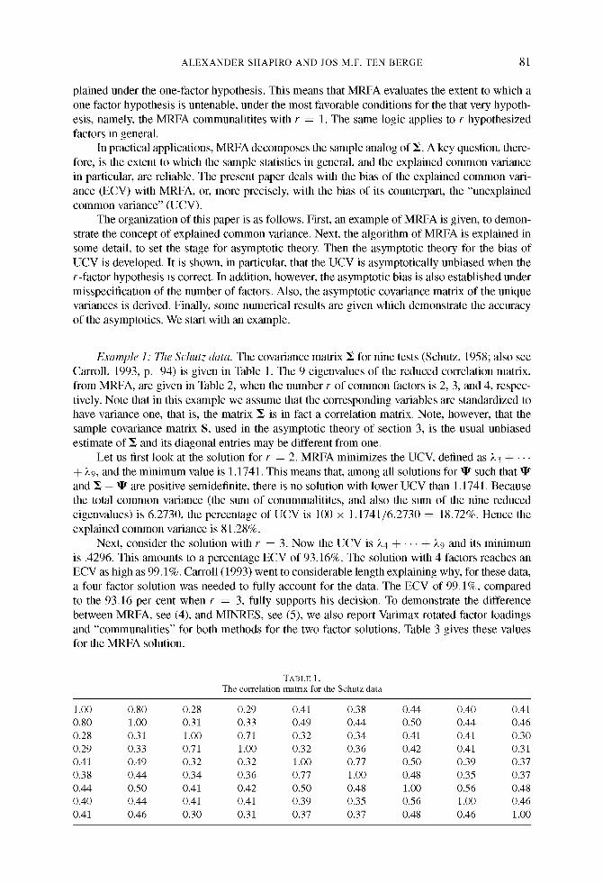
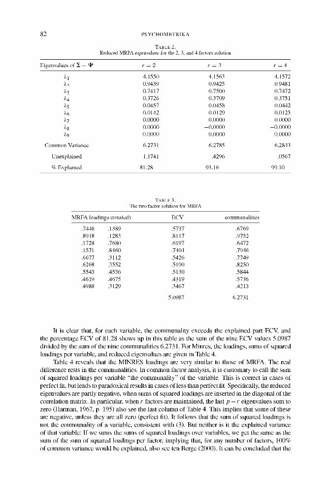
Example 1: The Schutz data. The covariance matrix 1~ for nine tests (Schutz, 1958; also see Carroll, 1993, p. 94) is given in Table 1. The 9 eigenvalues of the reduced correlation matrix, from MRFA, are given in Table 2, when the number r of common factors is 2, 3, and 4, respec- tively. Note that in this example we assume that the corresponding variables are standardized to have variance one, that is, the matrix ~ is in fact a correlation matrix. Note, however, that the sample covariance matrix S, used in the asymptotic theory of section 3, is the usual unbiased estimate of 1~ and its diagonal entries may be different from one.
Let us first look at the solution for r = 2. MRFA minimizes the UCV, defined as )~3 + " • + )~9, and the minimum value is 1.1741. This means that, among all solutions for ~It such that ~It and 1~ - ~It are positive semidefinite, there is no solution with lower UCV than 1.1741. Because the total common variance (the sum of communalitites, and also the sum of the nine reduced eigenvalues) is 6.2730, the percentage of UCV is 100 x 1.1741/6.2730 = 18.72%. Hence the explained common variance is 81.28%.
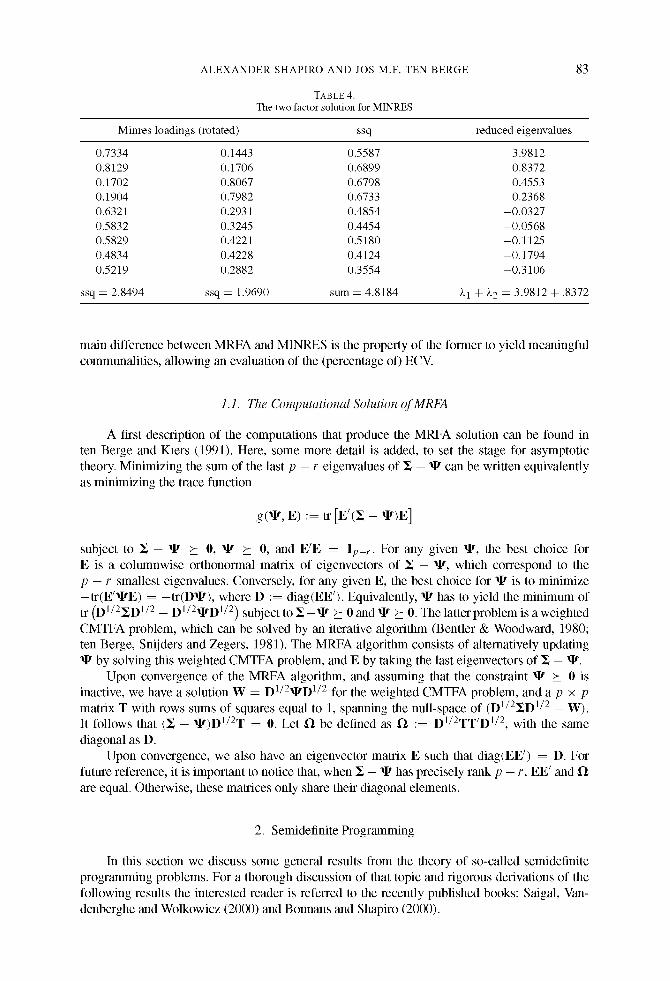
Next, consider the solution with r = 3. Now the UCV is ,~4 q- " ' " q- "~9 and its minimum is .4296. This amounts to a percentage ECV of 93.16%. The solution with 4 factors reaches an ECV as high as 99.1%. Carroll (1993) went to considerable length explaining why, for these data, a four factor solution was needed to fully account for the data. The ECV of 99.1%, compared to the 93.16 per cent when r = 3, fully supports his decision. To demonstrate the difference between MRFA, see (4), and MINRES, see (5), we also report Varimax rotated factor loadings and "communali t ies" for both methods for the two factor solutions. Table 3 gives these values for the MRFA solution.
TABLE 1. The correlation matrix for the Schutz data
1.00 0.80 0.28 0.29 0.41 0.38 0.44 0.40 0.41 0.80 1.00 0.31 0.33 0.49 0.44 0.50 0.44 0.46 0.28 0.31 1.00 0.71 0.32 0.34 0.41 0.41 0.30 0.29 0.33 0.71 1.00 0.32 0.36 0.42 0.41 0.31 0.41 0.49 0.32 0.32 1.00 0.77 0.50 0.39 0.37 0.38 0.44 0.34 0.36 0.77 1.00 0.48 0.35 0.37 0.44 0.50 0.41 0.42 0.50 0.48 1.00 0.56 0.48 0.40 0.44 0.41 0.41 0.39 0.35 0.56 1.00 0.46 0.41 0.46 0.30 0.31 0.37 0.37 0.48 0.46 1.00
82 PSYCHOMETRIKA
TABLE 2. Reduced MRFA eigenvalues for the 2, 3, and 4 factors solution
Eigenvalues of ]~ - xI* r = 2 r = 3 r = 4
~1 4.1550 4.1563 4.1572 ~2 0.9439 0.9425 0.9481 ~3 0.7417 0.7500 0.7472 ~4 0.3726 0.3709 0.3751 ~5 0.0457 0.0458 0.0442 ~6 0.0142 0.0129 0.0125 ~7 0.0000 0.0000 0.0000 ~8 0.0000 -0 .0000 -0 .0000 ~9 --0.0000 --0.0000 --0.0000
Common Vafiance 6.2731 6.2785 6.2843
Unexplmned 1.1741 .4296 .0567
%Explained 81.28 93.16 99.10
TABLE3. Thetwofactorsolutionfor MRFA
MRFA loadings (rotated) ECV communalities
.7446 .1389 .5737 .6769
.8918 .1283 .8117 .9752
.1728 .7680 .6197 .6472
.1571 .8460 .7404 .7946
.6677 .3112 .5426 .7749
.6268 .3552 .5190 .8250
.5543 .4536 .5130 .5844
.4619 .4675 .4319 .5736
.4988 .3129 .3467 .4213
5.0987 6.2731
It is clear that, for each variable, the communality exceeds the explained part ECV, and the percentage ECV of 81.28 shows up in this table as the sum of the nine ECV values 5.0987 divided by the sum of the nine communalities 6.2731. For Minres, the loadings, sums of squared loadings per variable, and reduced eigenvalues are given in Table 4.
Table 4 reveals that the MINRES loadings are very similar to those of MRFA. The real difference rests in the communalities. In common factor analysis, it is customary to call the sum of squared loadings per variable "the communality" of the variable. This is correct in cases of perfect fit, but leads to paradoxical results in cases of less than perfect fit. Specifically, the reduced eigenvalues are partly negative, when sums of squared loadings are inserted in the diagonal of the correlation matrix. In particular, when r factors are maintained, the last p - r eigenvalues sum to zero (Harman, 1967, p. 195) also see the last column of Table 4. This implies that some of these are negative, unless they are all zero (perfect fit). It follows that the sum of squared loadings is not the communality of a variable, consistent with (3). But neither is it the explained variance of that variable: If we sums the sums of squared loadings over variables, we get the same as the sum of the sum of squared loadings per factor, implying that, for any number of factors, 100% of common variance would be explained, also see ten Berge (2000). It can be concluded that the
A L E X A N D E R S H A P I R O AND JOS M.F. TEN B E R G E
TABLE 4. The two factor solution for MINRES
83
Minres loadings (rotated) ssq reduced eigenvalues
0.7334 0.1443 0.5587 3.9812 0.8129 0.1706 0.6899 0.8372 0.1702 0.8067 0.6798 0.4553 0.1904 0.7982 0.6733 0.2368 0.6321 0.2931 0.4854 -0.0327 0.5832 0.3245 0.4454 -0.0568 0.5829 0.4221 0.5180 -0.1125 0.4834 0.4228 0.4124 -0.1794 0.5219 0.2882 0.3554 -0.3106
ssq = 2.8494 ssq = 1.9690 sum= 4.8184 ~ 1 + ~ 2 = 3.9812 + .8372
main difference between MRFA and MINRES is the property of the former to yield meaningful communalities, allowing an evaluation of the (percentage of) ECV.
1.1. The Computational Solution of MRFA
A first description of the computations that produce the MRFA solution can be found in ten Berge and Kiers (1991). Here, some more detail is added, to set the stage for asymptotic theory. Minimizing the sum of the last p - r eigenvalues of 1~ - air can be written equivalently as minimizing the trace function
g(aIt, E) : = tr [E'(]~ - air)E]
subject to £ - xIt _~ 0, xIt _~ 0, and EIE = Ip-r. For any given xIt, the best choice for E is a columnwise orthonormal matrix of eigenvectors of £ - xIt, which correspond to the p - r smallest eigenvalues. Conversely, for any given E, the best choice for ~ is to minimize -tr(E1XItE) = -tr(DXP), where D := diag(EE~). Equivalently, xIt has to yield the minimum of tr (D1/2£D 1/2 - D1/2XItD 1/2) subject to £ - x I t _~ 0 and xIt _~ 0. The latter problem is a weighted
CMTFA problem, which can be solved by an iterative algorithm (Bentler & Woodward, 1980; ten Berge, Snijders and Zegers, 1981). The MRFA algorithm consists of alternatively updating xIt by solving this weighted CMTFA problem, and E by taking the last eigenvectors of ~ - xIt
Upon convergence of the MRFA algorithm, and assuming that the constraint ~ _~ 0 is inactive, we have a solution W = D1/2XItD 1/2 for the weighted CMTFA problem, and a p x p matrix T with rows sums of squares equal to 1, spanning the null-space of (D1/2£D 1/2 - W). It follows that (£ - xIt)D1/2T = 0. Let f~ be defined as f~ := DV2TT~D 1/2, with the same diagonal as D.
Upon convergence, we also have an eigenvector matrix E such that d iag(EE ~) = D. For future reference, it is important to notice that, when ~ - ~ has precisely rank p - r, E E ~ and f~ are equal. Otherwise, these matrices only share their diagonal elements.
2. Semidefinite Programming
In this section we discuss some general results from the theory of so-called semidefinite programming problems. For a thorough discussion of that topic and rigorous derivations of the following results the interested reader is referred to the recently published books: Saigal, Van- denberghe and Wolkowicz (2000) and Bonnans and Shapiro (2000).
84 PSYCHOMETRIKA
We use the following notation throughout the paper. By A t we denote the Moore-Penrose pseudo-inverse of matrix A, A • B denotes the Hadamard (i.e., term by term) product of matrices A and B, AGB denotes the Kronecker product of matrices A and B, Ip denotes the p x p identity matrix, vec(A) denotes vector obtained by stacking columns of matrix A, diag(H) denotes the vector formed by diagonal elements of matrix H, tr(H) denotes the trace of matrix H.
Let us consider the following optimization problem:
Min f(x) subject to G(x) _> 0. xE/~ m
(6)
Here f(x) is a real valued function of x E Nm, G(x) is a mapping from Nm into the space S p of p x p symmetric matrices, and
m {x E fl~m ,m} N + : = : x i > O , i = l . . . . .
Problems of the form (6) are called (nonlinear) semidefinite programming problems. For the sake of simplicity we consider the case where the constraint mapping G(x) is affine, i.e., G(x) :=
m A0 q- ~i=1 xiAi with A0, A1 . . . . . Am being given p x p symmetric matrices. MRFA can be considered in that framework if we use the objective function fmrfa (') and the constraint mapping G(x) := Z - X, where X is a diagonal matrix and x := diag(X). We refer to such mapping G(x) as FA-mapping.
Consider the set )/fs of p x p symmetric matrices of rank s. The set )/fs forms a smooth manifold in the linear space S p. We denote by TW~ (A) the tangent space to )/fs at A E )/Vs. A point 2 E Nm is said to be a feasible point of problem (6) if it satisfies the corresponding constraints, i.e., G(2) _~ 0 and 2 E N~. It is said that a feasible point 2 is nondegenerate if
m
£(~) + TW, (A) = S p, (7)
where s := rankG(2), A := G(~), I(~) := {i : xi = 0, i = 1 . . . . . m} and
/~(X) : = Z E S p : Z = x i A i , x i = O, i E I(~) .
i = 1
Note that both £(~) and Tws (A) are linear subspaces of SP, and that if I(2) is empty, i.e., all components of vector 2 are positive, then £(~) = DG(~)/7~ m. Here DG(~)h = ~i=lm hiAi is the differential of the mapping G and DG(~)]~ m is the image of the mapping DG(~) : ]~m __+ Sp"
It is known that
rw, (X) = {z e sp : ~.'z~. = 0}, (8)
where ~ = [~s+l . . . . . ~p] is a p x (p - s) matrix whose column vectors ~s+l . . . . . ~p form a
basis of the null space of the matrix A = G(~). We refer to = as a complement of the matrix A. Note that although the complement matrix ~ is not unique, the space given in the right hand side of the equation (8) is defined uniquely. In particular, one can take ~s+l . . . . . ~p to be a set
of orthonormal eigenvectors of A corresponding to its zero eigenvalue. By using this description of the tangent space it can be shown that condition (7) is equivalent
to the following condition. For s + 1 < k < ~ < p consider the (m - II (~)b-dimensional vectors with components ~ A i ~ . . . . i E { 1,. m} \ I (~). Then ~ is nondegenerate iff these vectors are linearly independent. Note that the total number of such vectors is (p - s) (p - s + 1)/2. Therefore a necessary condition for 2 to be nondegenerate is that
( p - s ) ( p - s + l ) ~ m - I I ( ~ ) l , (9)
where II (~) I denotes the number of elements in the set I (2).
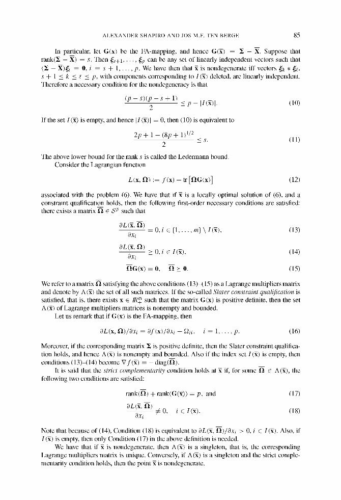
ALEXANDER SHAPIRO AND JOS M.F. TEN BERGE 85
m
In particular, let G(x) be the FA-mapping, and hence G(2) = X - X. Suppose that rank(X - X) = s. Then ~s+l . . . . . ~p can be any set of linearly independent vectors such that
(X - X)~i = 0, i = s + 1 . . . . . p. We have then that R is nondegenerate iff vectors ~k * ~e, s + 1 < k < g < p, with components corresponding to I (2) deleted, are linearly independent. Therefore a necessary condition for the nondegeneracy is that
( p - s ) ( p - s + l ) p - II(~)1. (10)
If the set I (~) is empty, and hence II (~)1 = 0, then (10) is equivalent to
2p + 1 - (8p + 1) 1/2 < s. (11)
The above lower bound for the rank s is called the Ledermann bound. Consider the Lagrangian function
L(x, 1~) := f (x ) -- tr [I~G(x)] (12)
associated with the problem (6). We have that if x is a locally optimal solution of (6), and a constraint qualification holds, then the following first-order necessary conditions are satisfied: there exists a matrix 1"1 E SP such that
m
OL(R, ~)
OXi - - 0 , i E {1 . . . . . m} \ I ( ~ ) ,
m
OL(R, ~)
OXi _>0, i E I (R) ,
m m
~ G ( ~ ) = 0 , ~ _ ~ 0 .
(13)
(14)
(15)
m
We refer to a matrix 1"1 satisfying the above conditions (13)-(15) as a Lagrange multipliers matrix and denote by A (3) the set of all such matrices. If the so-called Slater constraint qualification is satisfied, that is, there exists x E N ~ such that the matrix G(x) is positive definite, then the set A (2) of Lagrange multipliers matrices is nonempty and bounded.
Let us remark that if G(x) is the FA-mapping, then
OL(x, ~"~)/OXi = Of (x)/OXi + ~2ii, i = 1 . . . . . p. (16)
Moreover, if the corresponding matrix 1~ is positive definite, then the Slater constraint qualifica- tion holds, and hence A (2) is nonempty and bounded. Also if the index set I (R) is empty, then conditions (13)-(14) become V f (2 ) = - d iag(~) .
It is said that the strict complementarity condition holds at 2 if, for some ~ E A(~), the following two conditions are satisfied:
rank(~) + rank(G(~)) = p, and (17)
OL(~, [2) - - ¢ 0 , i E I ( ~ ) . (18)
Oxi
m
Note that because of (14), Condition (18) is equivalent to OL(~, ~)/Oxi > 0, i E I (~). Also, if I (~) is empty, then only Condition (17) in the above definition is needed.
We have that if ~ is nondegenerate, then A (~) is a singleton, that is, the corresponding Lagrange multipliers matrix is unique. Conversely, if A (~) is a singleton and the strict comple- mentarity condition holds, then the point ~ is nondegenerate.
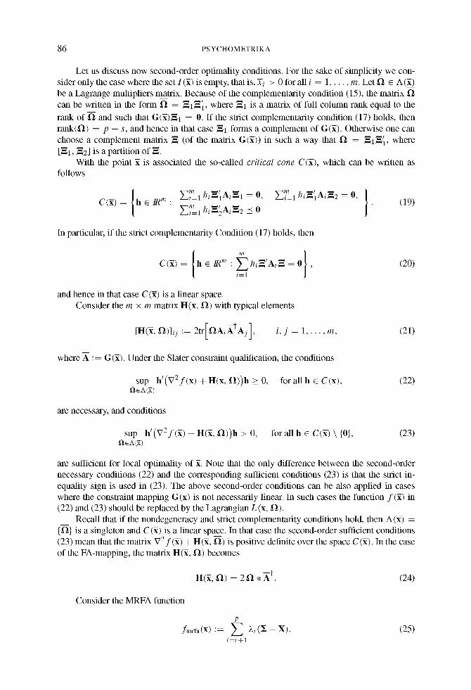
86 PSYCHOMETRIKA
Let us discuss now second-order optimality conditions. For the sake of simplicity we con- sider only the case where the set I (R) is empty, that is, xi > 0 for all i = 1 . . . . . m. Let I1 E A (~) be a Lagrange multipliers matrix. Because of the complementarity condition (15), the matrix I1 can be written in the form I1 = ~q~,~, where ~,1 is a matrix of full column rank equal to the
rank of f~ and such that G(~)~q = 0. If the strict complementarity condition (17) holds, then rank(O) = p - s, and hence in that case ~,1 forms a complement of G(~). Otherwise one can choose a complement matrix ~, (of the matrix G(~)) in such a way that I1 = ~q~,~, where [N~, N2] is a partition of N.
With the point ~ is associated the so-called critical cone C (~), which can be written as follows
~i=1 ~,2 0, ~i=1 ~-1 o, = hi~lAi = h i~ lAi C ( R ) = h E IN m: m
~ i = l ~t hi ~2Ai ~,2 _~ 0 (19)
In particular, if the strict complementarity Condition (17) holds, then
(20)
and hence in that case C (2) is a linear space. Consider the m x m matrix H(~, f~) with typical elements
[H(R, a ) ] i j := 2 t r [ a A i X ?Aj], i, j = 1 . . . . . m, (21)
m
where A := G(R). Under the Slater constraint qualification, the conditions
sup h ' (V2f(~) + H(~, f~))h _> 0, for all h E C(~), (22)
are necessary, and conditions
sup hz(V2f(x) ÷ H(~, f~))h > 0, for all h E C(~) \ {0}, (23)
are sufficient for local optimality of R. Note that the only difference between the second-order necessary conditions (22) and the corresponding sufficient conditions (23) is that the strict in- equality sign is used in (23). The above second-order conditions can be also applied in cases where the constraint mapping G(x) is not necessarily linear. In such cases the function f (~) in (22) and (23) should be replaced by the Lagrangian L(R, f~).
Recall that if the nondegeneracy and strict complementarity conditions hold, then A (2) = {I1} is a singleton and C (2) is a linear space. In that case the second-order sufficient conditions (23) mean that the matrix V 2 f (~) + H(~, f~) is positive definite over the space C (~). In the case of the FA-mapping, the matrix H(2, f~) becomes
H(~, f~) = 2 f~ • A?. (24)
Consider the MRFA function
fmrfa (X):= P
E i=r+l
~i ( :~ -x ) . (25)
A L E X A N D E R S H A P I R O A N D J O S M . F . T E N B E R G E 87
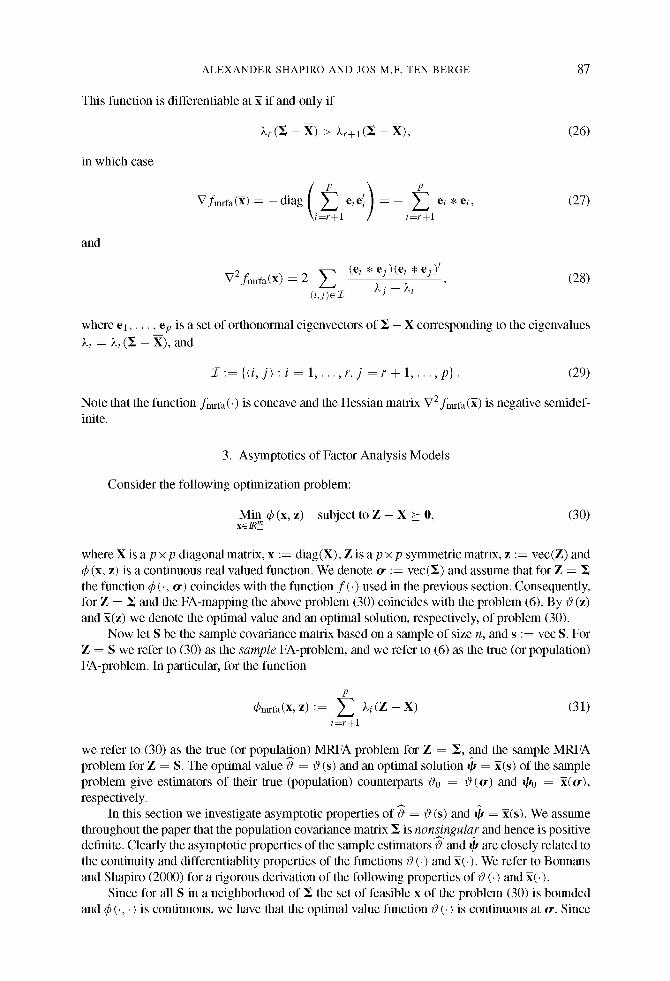
This function is differentiable at ~ if and only if
k~(~ -N) > k~+~(~ -N), (26)
in which case
V f m r f a ( X ) = - diag e i e = - - e i * e l ,
\ i = r + l / i = r + l
(27)
and
V2fmrfa(K) = 2 E (el * ej)(ei * e j ) I ( i , j ) c Z "~j - - "~i '
(28)
m
where el, . . . , ep is a set of orthonormal eigenvectors of 1~ - X corresponding to the eigenvalues
ki = ki (1~ - X), and
f : = { ( i , j ) : i = l . . . . . r , j = r + l . . . . . 1)}. (29)
Note that the function fmrfa(') is concave and the Hessian matrix V2 fmrfa(2) is negative semidef- inite.
3. Asymptotics of Factor Analysis Models
Consider the following optimization problem:
Min ~b (x, z) subject to Z - X _> O, (30) xE/~ m
where X is a p x p diagonal matrix, x := diag(X), Z is a p x p symmetric matrix, z := vec(Z) and ~b (x, z) is a continuous real valued function. We denote o- := vec(Z) and assume that for Z = the function ~b (., o-) coincides with the function f ( . ) used in the previous section. Consequently, for Z = Z and the FA-mapping the above problem (30) coincides with the problem (6). By O(z) and ~(z) we denote the optimal value and an optimal solution, respectively, of problem (30).
Now let S be the sample covariance matrix based on a sample of size n, and s := vec S. For Z = S we refer to (30) as the sample FA-problem, and we refer to (6) as the true (or population) FA-problem. In particular, for the function
P
qSmrfa(X,Z) := E ) ~ i ( Z - X ) (31) i = r + l
we refer to (30) as the true (or population) MRFA problem for Z = Z, and the sample MRFA problem for Z = S. The optimal value 0 = O(s) and an optimal solution ~ = 2(s) of the sample problem give estimators of their true (population) counterparts ~0 = 0(o-) and q~0 = ~(o-), respectively.
In this section we investigate asymptotic properties of O = 0 (s) and + = 2(s). We assume throughout the paper that the population covariance matrix Z is nonJngular and hence is positive definite. Clearly the asymptotic properties of the sample estimators 0 and qs are closely related to the continuity and differentiablity properties of the functions 0(.) and 2(.). We refer to Bonnans and Shapiro (2000) for a rigorous derivation of the following properties of 0 (.) and ~(.).
Since for all S in a neighborhood of Z the set of feasible x of the problem (30) is bounded and ~b (., .) is continuous, we have that the optimal value function 0(.) is continuous at o-. Since
88 PSYCHOMETRIKA
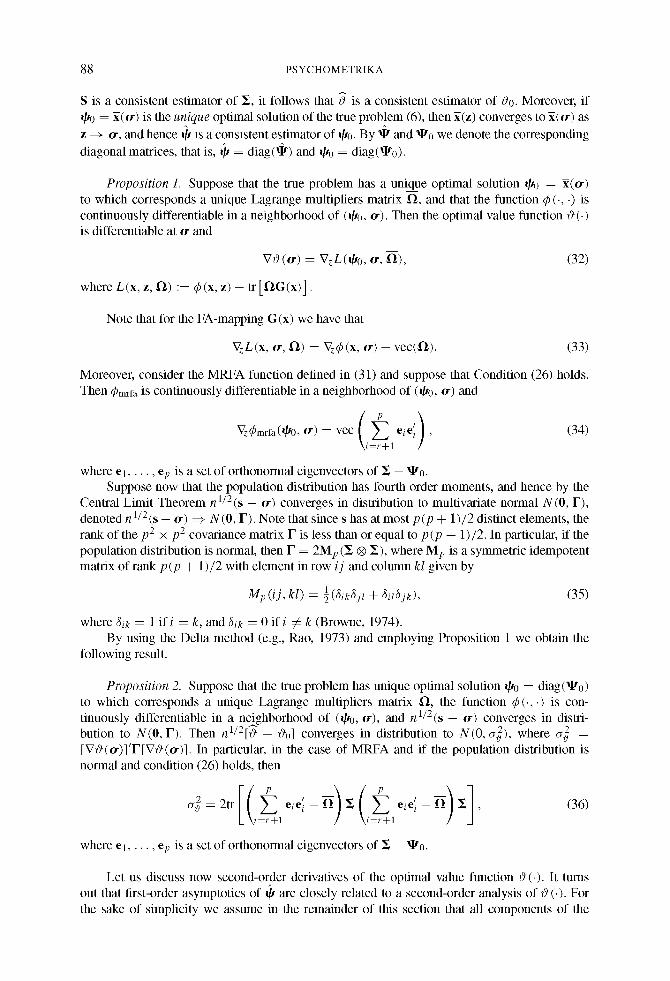
S is a consistent estimator of 1~, it follows that O is a consistent estimator of 00. Moreover, if too = 2(0-) is the unique optimal solution of the true problem (6), then 2(z) converges to 2(0-) as
z --+ or, and hence t} is a consistent estimator of too. By ~ and g 0 we denote the corresponding
diagonal matrices, that is, ~b = d iag(~) and too = diag(~0).
Proposition 1. Suppose that the true problem has a unique optimal solution too = 2(0-) to which corresponds a unique Lagrange multipliers matrix 1"1, and that the function ~b (., .) is continuously differentiable in a neighborhood of (too, 0% Then the optimal value function 0 (.) is differentiable at or and
m
VO(o-) = VzL(to0 , or, f~),
where L(x, z, f~) := qS(x, z) - tr [ f~G(x)] .
(32)
Note that for the FA-mapping G(x) we have that
VzL(x, or, f~) = Vzq5 (x, or) - vec(f~). (33)
Moreover, consider the MRFA function defined in (31) and suppose that Condition (26) holds. Then qSmrfa is continuously differentiable in a neighborhood of (too, or) and
Vz~,bmrfa(too, or) = vec eie , \ i = r + l /
(34)
where el, • • •, ep is a set of orthonormal eigenvectors of ]~ - air0. Suppose now that the population distribution has fourth order moments, and hence by the
Central Limit Theorem n 1/2 (s - or) converges in distribution to multivariate normal N (0, F), denoted nl/2(s - or) ~ N(0, F). Note that since s has at most p(p + 1)/2 distinct elements, the rank of the p2 x p2 covariance matrix F is less than or equal to p(p + 1)/2. In particular, if the population distribution is normal, then F = 2Mp (1~ ® 1~), where Mp is a symmetric idempotent matrix of rank p(p + 1)/2 with element in row ij and column kl given by
Mp (i j, kl) = 1 ((~ike~j I _}_ (~il(~jk), (35)
where 3ik = 1 if i = k, and 3ik = 0 if i ¢ k (Browne, 1974). By using the Delta method (e.g., Rao, 1973) and employing Proposition 1 we obtain the
following result.
Proposition 2. Suppose that the true problem has unique optimal solution tOo = diag(~0) to which corresponds a unique Lagrange multipliers matrix 1"1, the function ~b(., .) is con-
1/2 tinuously differentiable in a neighborhood of (too, or), and n (s - or) converges in distri- 1/2 bution to N(0, F). Then n [5 - 00] converges in distribution to N(0, oN), where oN =
[VO(~r)]T[VO(~r)]. In particular, in the case of MRFA and if the population distribution is normal and condition (26) holds, then
r( )1 a 2=2tr Z eieli-- ~ 1~ Z eieli-- ~ 1~ ' [_ \ i = r + l \ i = r + l
(36)
where el, • • •, ep is a set of orthonormal eigenvectors of 1~ - air0.
Let us discuss now second-order derivatives of the optimal value function 0(.). It turns out that first-order asymptotics of t~ are closely related to a second-order analysis of 0 (.). For the sake of simplicity we assume in the remainder of this section that all components of the
ALEXANDER SHAPIRO AND JOS M.F. TEN BERGE 89
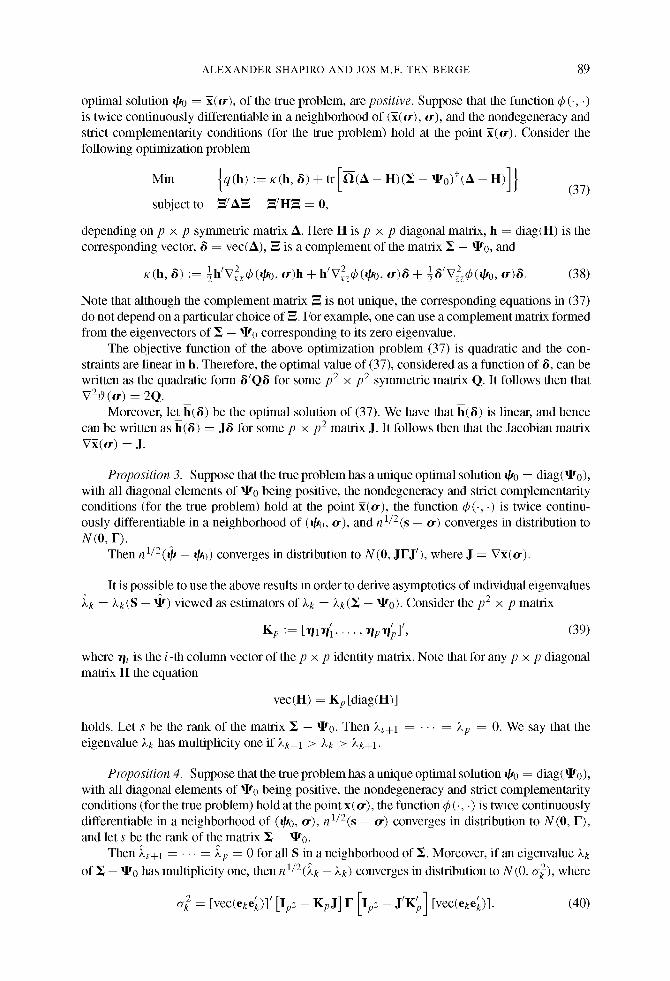
optimal solution too = 7(o-), of the true problem, are positive. Suppose that the function q5 (., .) is twice continuously differentiable in a neighborhood of (~(o-), o-), and the nondegeneracy and strict complementarity conditions (for the true problem) hold at the point 2(~r). Consider the following optimization problem
subject to NIAN - N ~ H N = 0,
depending on p x p symmetric matrix A Here 1t is p x p diagonal matrix, h = diag(lt) is the corresponding vector, ~ = vec(A), N is a complement of the matrix ~ - g 0 , and
l h t v / 2 ,6 t 2 1NtV/2 ~ x(h, ~) := ~ . . .xx . r ( too , o r ) h + h V x z ~ ( t o o , Or)~+ ~ .zz.r(too, Or)~. (38)
Note that although the complement matrix ~ is not unique, the corresponding equations in (37) do not depend on a particular choice of ~ . For example, one can use a complement matrix formed from the eigenvectors of ~ - g 0 corresponding to its zero eigenvalue.
The objective function of the above optimization problem (37) is quadratic and the con- straints are linear in h. Therefore, the optimal value of (37), considered as a function of 8, can be written as the quadratic form 6IQ6 for some p2 x p2 symmetric matrix Q It follows then that V20(or) = 2 Q
Moreover, let h(6) be the optimal solution of (37). We have that h(6) is linear, and hence can be written as h(6) = J 6 for some p x p2 matrix J. It follows then that the Jacobian matrix
Proposition 3. Suppose that the true problem has a unique optimal solution too = diag(XIt0), with all diagonal elements of xIt0 being positive, the nondegeneracy and strict complementarity conditions (for the true problem) hold at the point 2(o-), the function q5 (., .) is twice continu- ously differentiable in a neighborhood of (too, o-), and nl/2(s - o') converges in distribution to N (0, F).
Then n l / 2 ( ~ - too) converges in distribution to N(0, JFJI ) , where J = V2(o-).
It is possible to use the above results in order to derive asymptotics of individual eigenvalues
,~k = )~k(S -- ~ ) viewed as estimators of )~k = )~k(Z -- g 0 ) . Consider the p2 x p matrix
Kp := [aqlaq~ . . . . . aqpaq~]', (39)
where aqi is the i-th column vector of the p x p identity matrix. Note that for any p x p diagonal matrix H the equation
vec(H) = Kp [diag(H)]
holds. Let s be the rank of the matrix I~ - g 0 . Then )~s+l . . . . . Lp = 0. We say that the eigenvalue )~k has multiplicity one if )~k-1 > )~k > )~k+l.
Proposition 4. Suppose that the true problem has a unique optimal solution tOo = diag(XIt0), with all diagonal elements of xIt0 being positive, the nondegeneracy and strict complementarity conditions (for the true problem) hold at the point 2(o-), the function q5 (., .) is twice continuously differentiable in a neighborhood of (too, o-), nl/2(s - o') converges in distribution to N(0, F), and let s be the rank of the matrix Z - g 0 .
Then ~s+l . . . . . ,~p = 0 for all S in a neighborhood of Z Moreover, if an eigenvalue )~k
of Z -- g 0 has multiplicity one, then nl/2(~k -- )~k) converges in distribution to N(0, o-if), where
c~ff = [vec(eke~)]' [Ip2 - KpJ ] F [Ip2 - J ' K ~ ] [vec(eke~)]. (40)
90 PSYCHOMETRIKA
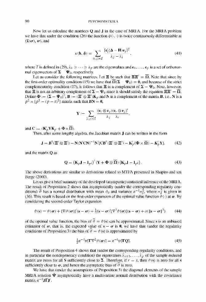
Now let us calculate the matrices Q and J in the case of MRFA. For the MRFA problem we have that under the condition (26) the function q5 (., .) is twice continuously differentiable at (2(o-), or), and
x(h, ~) = Z [e~i(A- H)ej]2 (41)
( i , j ) c Z , ~ j - - ,~i '
where ]7 is defined in (29),)vl _> . . . _> )Vp are the eigenvalues and el . . . . . ep is a set of orthonor- mal eigenvectors of £ - Rt0, respectively.
Let us consider the following matrices. Let N be such that NN~ = [1. Note that since by the first-order optimality condition (15) we have that [1(~ - Rt0) = 0, and because of the strict complementarity condition (17), it follows that N is a complement of ~ - R%. Note, however, that N is not an arbitrary complement of ~ - Rt0 since it should satisfy the equation NNI = [1. Define • := (~ - Rt0)*, B := (N~ ® ~t )Kp and N is a complement of the matrix B, i.e., N is a p2 x [p2 _ (p _ s)2] matrix such that BN = 0,
Y:= Z (ei®ej)(ei®ej) I ( i , j ) E Z L j - - L i '
m
and C := (K~YKp + • • ~ ) . Then, after some lengthy algebra, the Jacobian matrix J can be written in the form
J = B~(~ ' ® ~ ' ) - N ( N ' C N ) - I N ' [ C B ~ ( ~ ' ® ~ ' ) - K~ ((I) × ~ ) - K~Y], (42)
and the matrix Q as
Q = (KpJ - Ip2)' (Y + • ® ~ ) (KpJ - Ip2). (43)
The above derivations are similar to derivations related to MTFA presented in Shapiro and ten Berge (2000).
Let us give a brief summary of the developed (asymptotic) statistical inference of the MRFA. The result of Proposition 2 shows that asymptotically (under the corresponding regularity con- ditions) O has a normal distribution with mean O0 and variance n - l c @ where o-g is given in (36). This result is based on the first-order expansion of the optimal value function 0 (.) at or. By considering the second-order Taylor expansion
O(s) = o ( o - ) + W ~ ( o - ) ] 1 ( s - o-) + ~ ( s - o - ) 1 W 2 ~ ( o - ) ] ( s - o-) + o( l l s - oII 2) (44)
of the optimal value function, the bias o f O = O(s) can be approximated. Since s is an unbiased estimator of or, that is, the expected value of s - or is 0, we have that (under the regularity conditions of Proposition 3) the bias of 0 = 0 (s) is approximated by
½n-ltr[FVeO(o-)] = n - l t r [FQ] . (45)
The result of Proposition 4 shows that (under the corresponding regularity conditions, and in particular the nondegeneracy condition) the eigenvalues ,~s+l . . . . . 2p of the sample reduced matrix are zeros for all S sufficiently close to Z Therefore, if r = s, then 0 (s) is zero for all s sufficiently close to or, and hence the asymptotic bias of 0 is zero.
We have that (under the assumptions of Proposition 3) the diagonal elements of the sample
MRFA solution ~ asymptotically have a multivariate normal distribution with the covariance matrix n - 1JFJ ' .
ALEXANDER SHAPIRO AND JOS M.F. TEN BERGE 91
3.1. A Numerical Example
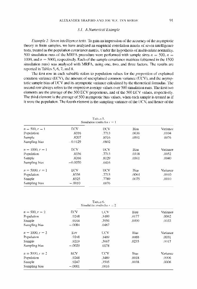
Example 2: Seven intelligence tests. To gain an impression of the accuracy of the asymptotic
theory in finite samples, we have analyzed an empirical correlation matrix of seven intelligence
tests, treated as the population covariance matrix. Under the hypothesis of multivariate normality,
500 simulation runs of the MRFA procedure were performed with sample sizes n = 500, n =
1000, and n = 5000, respectively. Each of the sample covariance matrices (obtained in the 1500
simulation runs) was analyzed with MRFA, using one, two, and three factors. The results are
reported in Tables 5, 6, 7, and 8.
The first row in each subtable refers to population values for the proportion of explained
common variance (ECV), the amount of unexplained common variance (UCV), and the asymp-
totic sample bias of UCV and its asymptotic variance calculated by the theoretical formulas. The
second row always refers to the respective average values over 500 simulation runs. The first two
elements are the average of the 500 ECV proportions, and of the 500 ECV values, respectively.
The third element is the average of 500 asymptotic bias values, when each sample is treated as if
it were the population. The fourth element is the sampling variance of the UCV, and hence of the
TABLE 5. Simulation results for r = 1
n = 500, r = 1 ECV UCV Bias Variance Population .8336 .7713 .0636 .0104 Sample .8207 .8516 .0591 .0076 Sampling bias -0.0129 .0802
n = 1000, r = 1 ECV UCV Bias Variance Population .8336 .7713 .0318 .0052 Sample .8266 .8129 .0361 .0040 Sampling bias -0.0070 .0416
n = 5000, r = 1 ECV UCV Bias Variance Population .8336 .7713 .0064 .0010 Sample .8325 .7789 .0075 .0010 Sampling bias -.0010 .0076
TABLE 6. Simulation results for r = 2
n = 500, r = 2 ECV UCV Bias Variance Population .9248 .3489 .0177 .0062 S ample .9164 .3956 .0490 .0033 Sampling bias -.0084 .0467
n = 1000, r = 2 Ecv UCV Bias Variance Population .9248 .3489 .0088 .0031 Sample .9219 .3667 .0235 .0017 Sampling bias -.0029 .0178
n = 5000, r = 2 ECV UCV Bias Variance Population .9248 .3489 .0018 .0006 Sample .9247 .3505 .0038 .0006 Sampling bias -.0001 .0016
92 PSYCHOMETRIKA
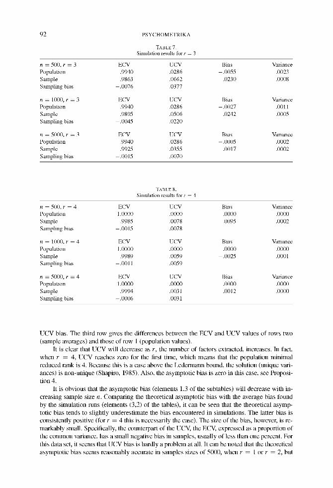
TABLE 7. Simulation results for r = 3
n = 500, r = 3 ECV UCV Bias Variance Population .9940 .0286 -.0055 .0023 Sample .9863 .0662 .0230 .0008 Sampling bias -.0076 .0377
n = 1000, r = 3 ECV UCV Bias Variance Population .9940 .0286 -.0027 .0011 Sample .9895 .0506 .0242 .0005 Sampling bias -.0045 .0220
n = 5000, r = 3 ECV UCV Bias Variance Population .9940 .0286 -.0005 .0002 Sample .9925 .0355 .0017 .0002 Sampling bias -.0015 .0070
TABLE 8. Simulation results for r = 4
n = 500, r = 4 ECV UCV Bias Variance Population 1.0000 .0000 .0000 .0000 Sample .9985 .0078 .0095 .0002 Sampling bias -.0015 .0078
n = 1000, r = 4 ECV UCV Bias Variance Population 1.0000 .0000 .0000 .0000 Sample .9989 .0059 -.0025 .0001 Sampling bias -.0011 .0059
n = 5000, r = 4 ECV UCV Bias Variance Population 1.0000 .0000 .0000 .0000 S ample .9994 .0031 .0012 .0000 Sampling bias -.0006 .0031
UCV bias. The third row gives the differences between the ECV and UCV values of rows two
(sample averages) and those of row 1 (population values).
It is clear that UCV will decrease as r, the number of factors extracted, increases. In fact,
when r = 4, UCV reaches zero for the first time, which means that the population minimal
reduced rank is 4. Because this is a case above the Ledermann bound, the solution (unique vari-
ances) is non-unique (Shapiro, 1985). Also, the asymptotic bias is zero in this case, see Proposi-
tion 4.
It is obvious that the asymptotic bias (elements 1,3 of the subtables) will decrease with in-
creasing sample size n. Comparing the theoretical asymptotic bias with the average bias found
by the simulation runs (elements (3,2) of the tables), it can be seen that the theoretical asymp-
totic bias tends to slightly underestimate the bias encountered in simulations. The latter bias is
consistently positive (for r = 4 this is necessarily the case). The size of the bias, however, is re-
markably small. Specifically, the counterpart of the UCV, the ECV, expressed as a proportion of
the common variance, has a small negative bias in samples, usually of less than one percent. For
this data set, it seems that UCV bias is hardly a problem at all. It can be noted that the theoretical
asymptotic bias seems reasonably accurate in samples sizes of 5000, when r = 1 or r = 2, but
A L E X A N D E R SHAPIRO AND JOS M.F. TEN BERGE
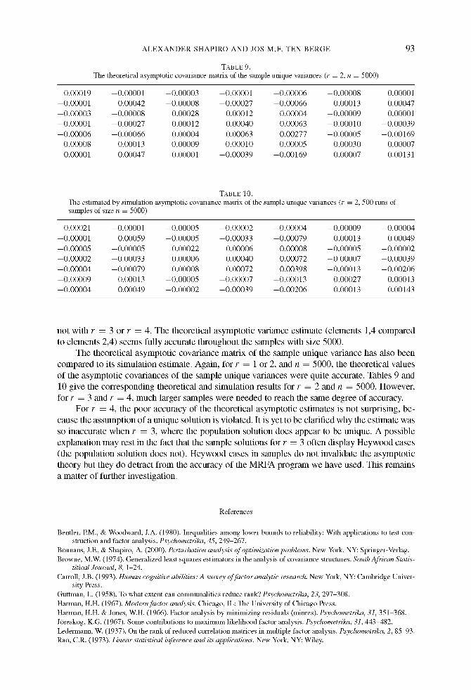
TABLE 9. The theoretical asymptotic covariance matrix of the sample unique variances (r = 2, n = 5000)
93
0.00019 --0.00001 - -0 .00003 - -0 .00001 - -0 .00006 - -0 .00008 0.00001
--0 .00001 0.00042 - -0 .00008 - -0 .00027 - -0 .00066 0.00013 0.00047
- -0 .00003 - -0 .00008 0.00028 0.00012 0 .00004 - -0 .00009 0.00001
--0 .00001 - -0 .00027 0 .00012 0.00040 0.00063 - -0 .00010 - -0 .00039
- -0 .00006 - -0 .00066 0 .00004 0.00063 0.00277 - -0 .00005 - -0 .00169
- -0 .00008 0.00013 - -0 .00009 - -0 .00010 - -0 .00005 0 .00030 0.00007
0.00001 0.00047 0.00001 - -0 .00039 - -0 .00169 0.00007 0.00131
TABLE 10. The estimated by simulation asymptotic covaxiance matrix of the sample unique samples of size n = 5000)
variances (r = 2, 500 runs of
0.00021 - 0 . 0 0 0 0 1 - 0 . 0 0 0 0 5 - 0 . 0 0 0 0 2 - 0 . 0 0 0 0 4 - 0 . 0 0 0 0 9 - 0 . 0 0 0 0 4
- 0 . 0 0 0 0 1 0.00059 - 0 . 0 0 0 0 5 - 0 . 0 0 0 3 3 - 0 . 0 0 0 7 9 0.00013 0.00049
- 0 . 0 0 0 0 5 - 0 . 0 0 0 0 5 0 .00022 0.00006 0.00008 - 0 . 0 0 0 0 5 - 0 . 0 0 0 0 2
- 0 . 0 0 0 0 2 - 0 . 0 0 0 3 3 0.00006 0.00040 0 .00072 - 0 . 0 0 0 0 7 - 0 . 0 0 0 3 9
- 0 . 0 0 0 0 4 - 0 . 0 0 0 7 9 0.00008 0.00072 0.00398 - 0 . 0 0 0 1 3 - 0 . 0 0 2 0 6
- 0 . 0 0 0 0 9 0.00013 - 0 . 0 0 0 0 5 - 0 . 0 0 0 0 7 - 0 . 0 0 0 1 3 0.00027 0.00013
- 0 . 0 0 0 0 4 0.00049 - 0 . 0 0 0 0 2 - 0 . 0 0 0 3 9 - 0 . 0 0 2 0 6 0.00013 0.00143
not with r = 3 or r = 4. The theoretical asymptotic variance estimate (elements 1,4 compared to elements 2,4) seems fully accurate throughout the samples with size 5000.
The theoretical asymptotic covariance matrix of the sample unique variance has also been compared to its simulation estimate. Again, for r = 1 or 2, and n = 5000, the theoretical values of the asymptotic covariances of the sample unique variances were quite accurate. Tables 9 and 10 give the corresponding theoretical and simulation results for r = 2 and n = 5000. However, for r = 3 and r = 4, much larger samples were needed to reach the same degree of accuracy.
For r = 4, the poor accuracy of the theoretical asymptotic estimates is not surprising, be- cause the assumption of a unique solution is violated. It is yet to be clarified why the estimate was so inaccurate when r = 3, where the population solution does appear to be unique. A possible explanation may rest in the fact that the sample solutions for r = 3 often display Heywood cases (the population solution does not). Heywood cases in samples do not invalidate the asymptotic theory but they do detract from the accuracy of the MRFA program we have used. This remains a matter of further investigation.
References
Bentler, RM., & Woodward, J.A. (1980). Inequalities among lower bounds to reliability: With applications to test con- struction and factor analysis. Psychometrika, 45, 249-267.
Bonnans, J.F., & Shapiro, A. (2000). Perturbation analysis of optimization problems. New York, NY: Springer-Verlag. Browne, M.W. (1974). Generalized least squares estimators in the analysis of covariance structures. South African Statis-
titical Journal, 8, 1-24. Carroll, J.B. (1993). Human cognitive abilities: A survey of factor analytic research. New York, NY: Cambridge Univer-
sity Press. Guttman, L. (1958). To what extent can communalities reduce rank? Psychometrika, 23, 297-308. Harman, H.H. (1967). Modern factor analysis. Chicago, IL: The University of Chicago Press. Harman, H.H. & Jones, W.H. (1966). Factor analysis by minimizing residuals (minres). Psychometrika, 31, 351-368. J6reskog, K.G. (1967). Some contributions to maximum likelihood factor analysis. Psychometrika, 31,443-482. Ledermann, W. (1937). On the rank of reduced correlation matrices in multiple factor analysis. Psychometrika, 2, 85-93. Rao, C.R. (1973). Linear statistical inference and its applications. New York, NY: Wiley.
94 PSYCHOMETRIKA
SaJgal, R., Vandenberghe, L. & Wolkowicz, H. (Eds.). (2000). Semidefinite programming and applications handbook. Boston, MA: Kluwer Academic Publishers.
Schutz, R.E. (1958). Factorial validity of the Holzinger-Crowder Uni-Factor Tests. Educational and Psychological Mea- surement, 18, 873-875.
Shapiro, A. (1982). Rank reducibility of a symmetric matrix and sampling theory of minimum trace factor analysis. Psychometrika, 47, 187-199.
Shapiro, A. (1985). Identifiability of factor analysis: Some results and open problems. Linear Algebra and its Applica- tions, 70, 1-7.
Shapiro, A. & ten Berge, J.M.F. (2000). The asymptotic bias of Minimum Trace Factor Analysis, with applications to the greatest lower bound to reliability. Psychometrika, 65, 413-425.
ten Berge, J.M.E (1998). Some recent developments in factor analysis and the search for proper communalities. In A. Rizzi, M. Vichi, & H.H. Bock (Eds), Advances in data science and classification (pp. 325-334). Heidelberg, Germany: Springer.
ten Berge, J.M.F. (2000). Linking reliability and factor analysis:recent developments in some classical psychometric problems. In S.E. Hampson (Ed.), Advances in personality psychology, Vol. 1 (pp. 138-156). London, England: Routledge.
ten Berge, J.M.F. & Kiers, H.A.L. (1991). A numerical approach to the exact and the approximate minimum rank of a covariance matrix. Psychometrika, 56, 309-315.
ten Berge, J.M.F., Snijders, T.A.B. & Zegers, EE. (1981). Computational aspects of the greatest lower bound to reliability and constrained minimum trace factor analysis. Psychometrika, 46, 201-213.