Psych 5500/6500

1

Psych 5500/6500

Introduction to the F Statistic

(Segue to ANOVA)

Fall, 2008

2

Overview of the F test

The F test is used in many contexts. We will begin by taking a general look at how the F test works.

In its most general form, the F test is used to determine whether two populations have the same variance.

3

Example

We know that the mean height of men is greater than the mean height of females, but what about their respective variances? (two-tail example)

H0: σ²Female = σ²Male

HA: σ²Female σ²Male

4

Test Statistic

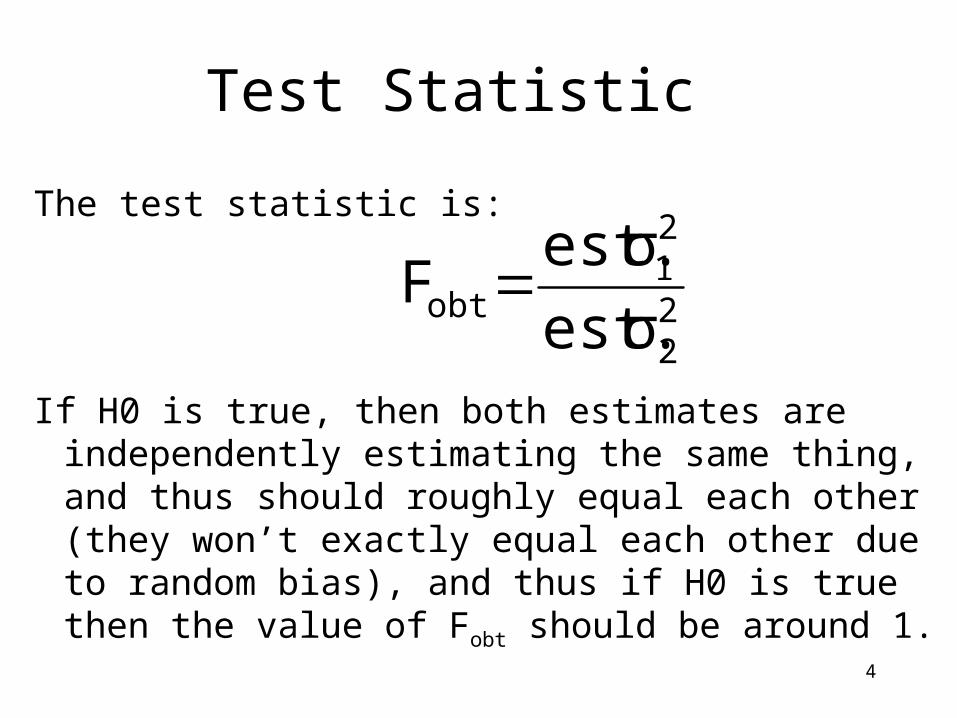
The test statistic is:

If H0 is true, then both estimates are independently estimating the same thing, and thus should roughly equal each other (they won’t exactly equal each other due to random bias), and thus if H0 is true then the value of Fobt should be around 1.

22

21

obt est.σ

est.σF

5

Degrees of Freedom

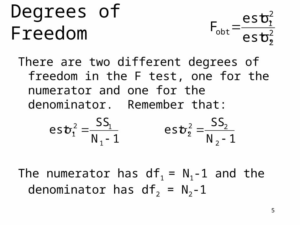
There are two different degrees of freedom in the F test, one for the numerator and one for the denominator. Remember that:

The numerator has df1 = N1-1 and the denominator has df2 = N2-1

22

21

obt est.σ

est.σF

1N

SSest.

1

121

1N

SSest.

2

222

6

Expected (Mean) Value of F

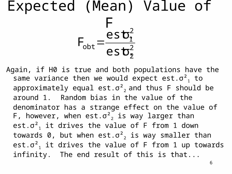
Again, if H0 is true and both populations have the same variance then we would expect est.σ²1 to approximately equal est.σ²2 and thus F should be around 1. Random bias in the value of the denominator has a strange effect on the value of F, however, when est.σ²2 is way larger than est.σ²1 it drives the value of F from 1 down towards 0, but when est.σ²2 is way smaller than est.σ²1 it drives the value of F from 1 up towards infinity. The end result of this is that...

22

21

obt est.σ

est.σF

7


22

21

obt est.σ

est.σF

2)(df

dfμ : trueis H0When

2

2F

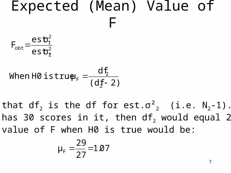
Remember that df2 is the df for est.σ²2 (i.e. N2-1). Thus ifsample 2 has 30 scores in it, then df2 would equal 29, andthe mean value of F when H0 is true would be:

07.127

29μF

8


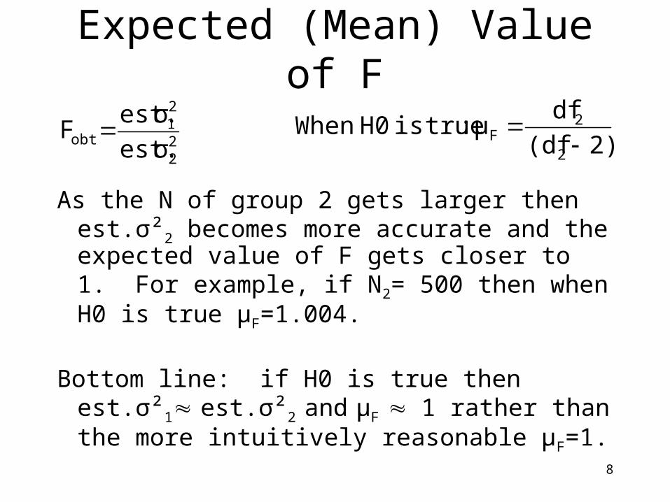
As the N of group 2 gets larger then est.σ²2 becomes more accurate and the expected value of F gets closer to 1. For example, if N2= 500 then when H0 is true μF=1.004.

Bottom line: if H0 is true then est.σ²1 est.σ²2

and μF 1 rather than the more intuitively reasonable μF=1.

22

21

obt est.σ

est.σF

2)(df

dfμ : trueis H0When

2

2F

9

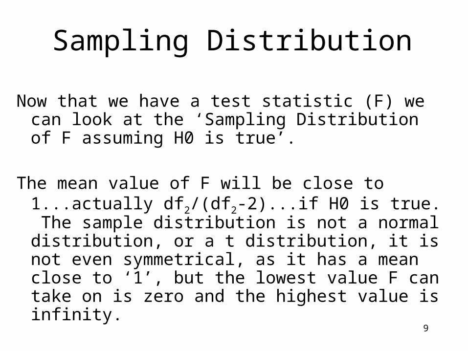
Sampling Distribution

Now that we have a test statistic (F) we can look at the ‘Sampling Distribution of F assuming H0 is true’.

The mean value of F will be close to 1...actually

df2/(df2-2)...if H0 is true. The sample distribution is not a normal distribution, or a t distribution, it is not even symmetrical, as it has a mean close to ‘1’, but the lowest value F can take on is zero and the highest value is infinity.

10

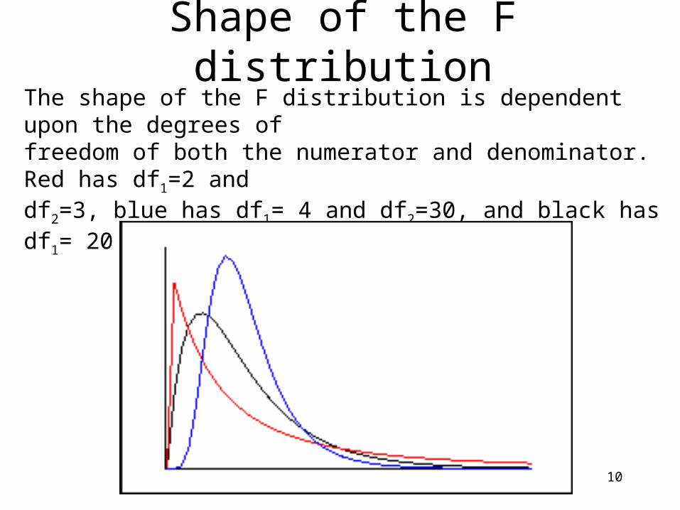
Shape of the F distributionThe shape of the F distribution is dependent upon the degrees of freedom of both the numerator and denominator. Red has df1=2 and df2=3, blue has df1= 4 and df2=30, and black has df1= 20 and df2=20.

11

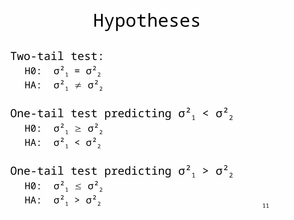
Hypotheses

Two-tail test:H0: σ²1 = σ²2

HA: σ²1 σ²2

One-tail test predicting σ²1 < σ²2

H0: σ²1 σ²2

HA: σ²1 < σ²2

One-tail test predicting σ²1 > σ²2

H0: σ²1 σ²2

HA: σ²1 > σ²2

12

Fc values

As the shape of the F distribution changes with different degrees of freedom, you need to know both df to find the Fc values.

Remember:df1 (i.e. for the numerator of F)= N-1 for est. σ²1

df2 (i.e. for the denominator of F) = N-1 for est. σ²2

13

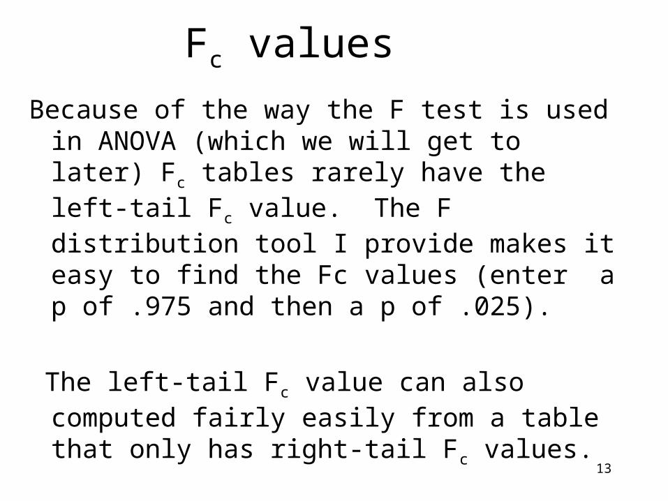
Fc values

Because of the way the F test is used in ANOVA (which we will get to later) Fc tables rarely have the left-tail Fc value. The F distribution tool I provide makes it easy to find the Fc values (enter a p of .975 and then a p of .025).

The left-tail Fc value can also computed fairly easily from a table that only has right-tail Fc values.

14

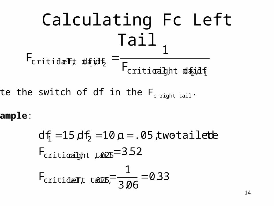
Calculating Fc Left Tail

12

21df,df:right tail critical,

df,df:left tail critical, F

1F

Note the switch of df in the Fc right tail.

Example:

33.006.3

1F

52.3F

testtailed- two.05,α 10,df 15,df

.025 left tail, critical,

.025 ,right tail critical,

21

15

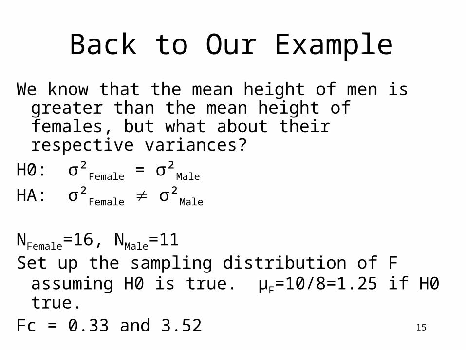
Back to Our Example

We know that the mean height of men is greater than the mean height of females, but what about their respective variances?

H0: σ²Female = σ²Male


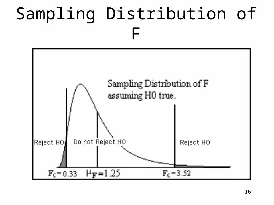
NFemale=16, NMale=11Set up the sampling distribution of F assuming H0

is true. μF=10/8=1.25 if H0 true. Fc = 0.33 and 3.52

16

Sampling Distribution of F

17

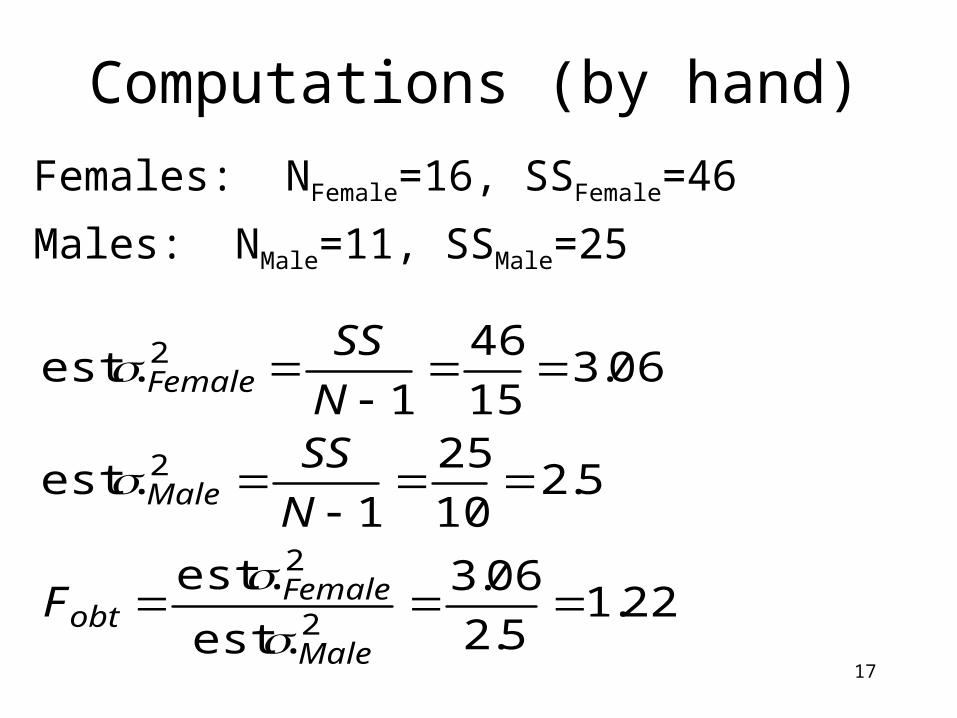
Computations (by hand)

Females: NFemale=16, SSFemale=46

Males: NMale=11, SSMale=25

22.15.2

06.3

est.

est.

5.210

25

1 est.

06.315

46

1 est.

2

2

2

2

Male

Femaleobt

Male

Female

F

N

SSN

SS

18

Computations SPSS

While SPSS doesn’t provide this use of the F test it will provide the ‘Variance’ of each group. Remember that in SPSS the ‘Variance’ of a group is actually the est. σ² of the population from which the sample was drawn, which is just what we need to compute F. You will still, however, need an F table to come up with the Fcritical values.

19

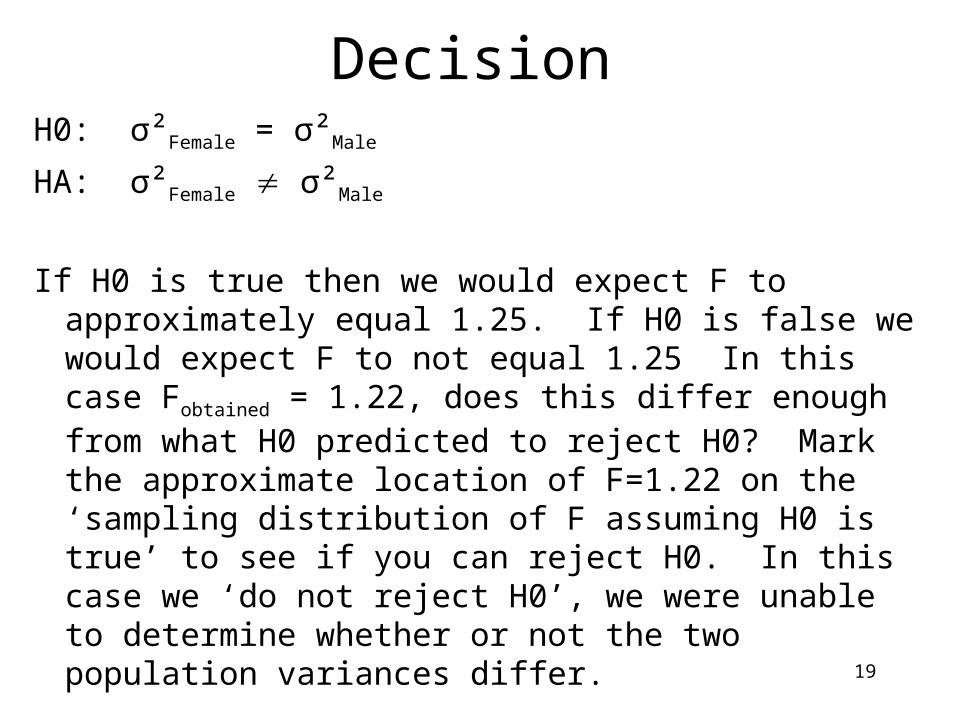
DecisionH0: σ²Female = σ²Male


If H0 is true then we would expect F to approximately equal 1.25. If H0 is false we would expect F to not equal 1.25 In this case Fobtained = 1.22, does this differ enough from what H0 predicted to reject H0? Mark the approximate location of F=1.22 on the ‘sampling distribution of F assuming H0 is true’ to see if you can reject H0. In this case we ‘do not reject H0’, we were unable to determine whether or not the two population variances differ.

20

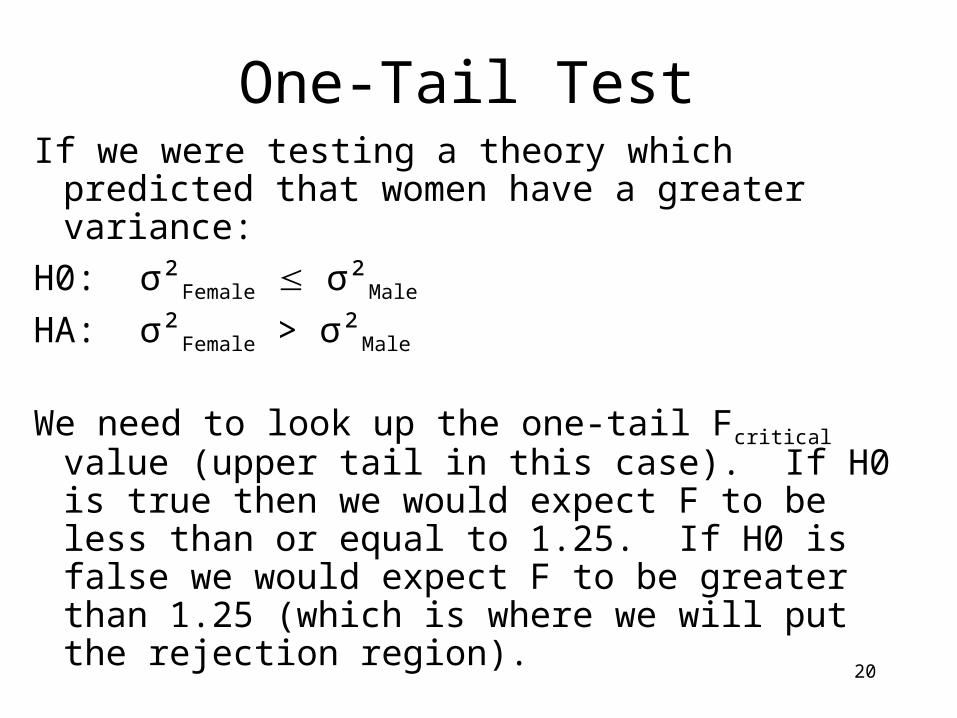
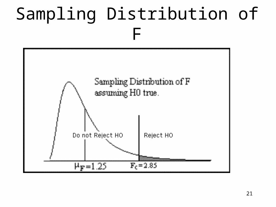
One-Tail TestIf we were testing a theory which predicted that

women have a greater variance:

H0: σ²Female σ²Male

HA: σ²Female > σ²Male

We need to look up the one-tail Fcritical value (upper tail in this case). If H0 is true then we would expect F to be less than or equal to 1.25. If H0 is false we would expect F to be greater than 1.25 (which is where we will put the rejection region).

21


22

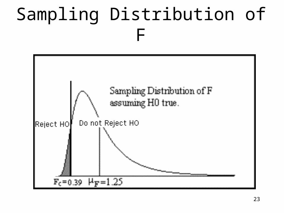
One-Tail TestIf we were testing a theory which predicted that

women have lesser variance:

H0: σ²Female σ²Male

HA: σ²Female < σ²Male

We need to look up the one-tail Fcritical value (lower tail in this case). If H0 is true then we would expect F to be greater than or equal to 1.25. If H0 is false we would expect F to be less than 1.25 (which is where we will put the rejection region).

23


24

Assumptions of this Use of F

1. The two variance estimates are independent of each other.

2. Both populations are normally distributed. Monte Carlo studies have shown that this assumption is quite important for the validity of this test.

25

Back to the Assumptions of the t Test

One of the assumptions of the t test for independent means is that the variances of the two populations are equal. The F test we have just covered can test that assumption. But remember, due to the nature of null hypothesis testing, we can prove two variances are different but we can’t prove two variances are equal, because we can’t prove that H0 is true (unless we can show we have a powerful experiment, which would make beta small). The affect that non-normality has on the validity of this F test has led to it not being used as much as Levene’s test (mentioned next).

26

Levene’s Test

Levene’s test is another way to determine whether or not the population variances are the same. Levene’s test has two advantages over the F test we just covered. First, it is less dependent upon the populations being normally distributed. Second, it can be used to test whether several groups all have the same variance.

H0: σ²1 = σ²2 = σ²3 …

HA: at least one σ² is different than the rest.

We will cover Levene’s test and how it works soon.

Documents

Psych 5500/6500