Psych 5500/6500

Probability

Fall, 2008

Gambler’s Fallacy

The “gambler’s fallacy” is to think that the “law of averages” makes independent events no longer independent. For example, on flipping a fair coin, to think that if you get five heads in a row then the probability of getting a tail next is greater due to the ‘law of averages’ is to make the gamblers fallacy.

Basics1) p(A) = probability of event ‘A’

occurring2) 0 p(A) 1.00 (p=0 means that A is an ‘impossible’ event,

p=1.00 means that A is a ‘sure’ event, probability cannot be less than 0 or greater than 1.00)

3) p(~A) stands for probability of ‘not A’4) p(A) + p(~A) = 1.00 (this is because A and ~A are mutually exclusive

and exhaustive)

Alternative Viewpoint

For an interesting alternative viewpoint on the usefulness of dividing the world into A and ~A, see:

Kosko, B. (1993) Fuzzy Thinking: The New Science of Fuzzy Logic. New York: Hyperion.

...but we digress

Theoretical Probability

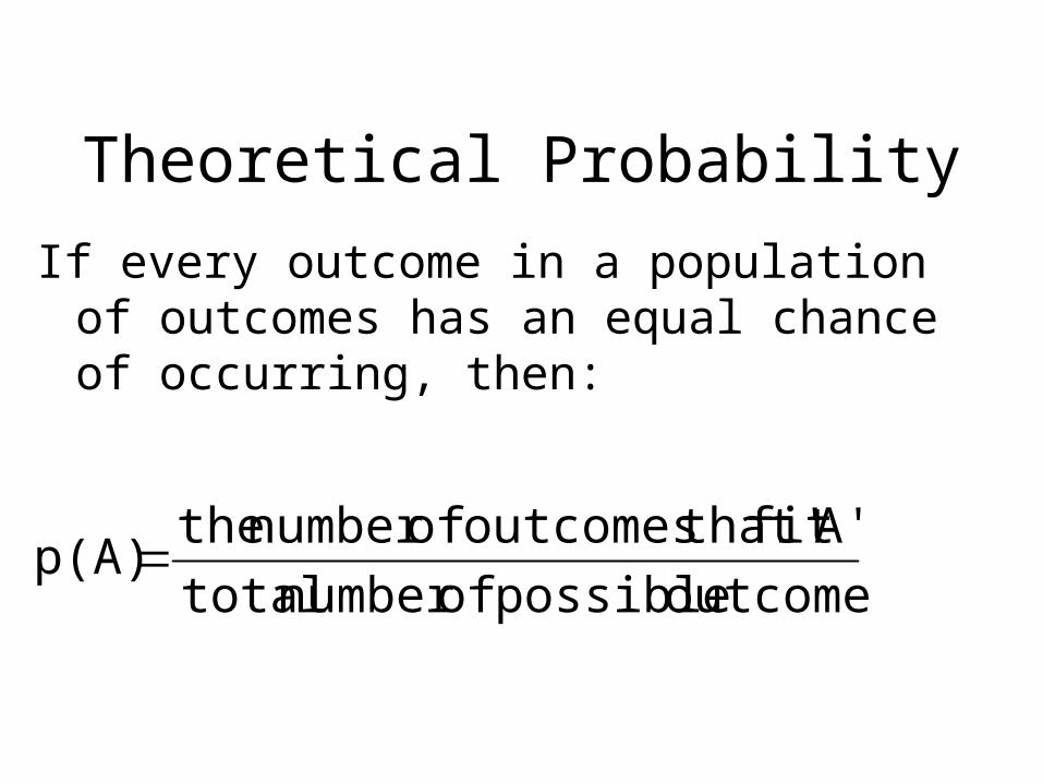
If every outcome in a population of outcomes has an equal chance of occurring, then:

outcomes possible ofnumber total

A''fit that outcomes ofnumber the p(A)

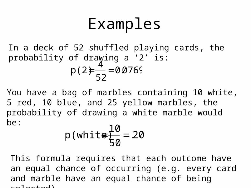
ExamplesIn a deck of 52 shuffled playing cards, the probability of drawing a ‘2’ is:

0769.052

4 p(2)

You have a bag of marbles containing 10 white, 5 red, 10 blue, and 25 yellow marbles, the probability of drawing a white marble would be:

20.50

10 p(white)

This formula requires that each outcome have an equal chance of occurring (e.g. every card and marble have an equal chance of being selected).

Empirical Probability

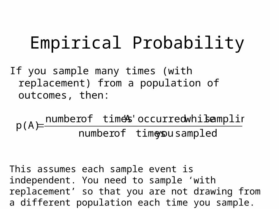
If you sample many times (with replacement) from a population of outcomes, then:

sampledyou timesofnumber

sampling whileoccurred A'' timesofnumber p(A)

This assumes each sample event is independent. You need to sample ‘with replacement’ so that you are not drawing from a different population each time you sample.

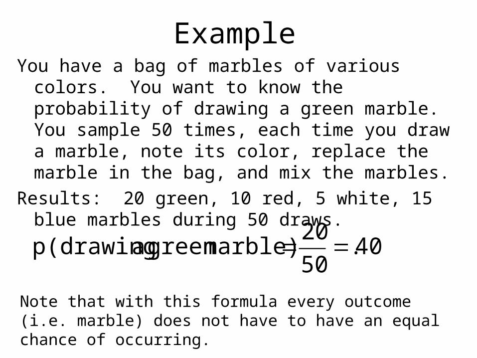
ExampleYou have a bag of marbles of various colors. You

want to know the probability of drawing a green marble. You sample 50 times, each time you draw a marble, note its color, replace the marble in the bag, and mix the marbles.

Results: 20 green, 10 red, 5 white, 15 blue marbles during 50 draws.

40.50

20marble)green a p(drawing

Note that with this formula every outcome (i.e. marble) does not have to have an equal chance of occurring.

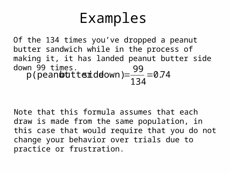
ExamplesOf the 134 times you’ve dropped a peanut butter sandwich while in the process of making it, it has landed peanut butter side down 99 times.

74.0134

99down) sidebutter p(peanut

Note that this formula assumes that each draw is made from the same population, in this case that would require that you do not change your behavior over trials due to practice or frustration.

Conditional Probability

p(A|B) = the probability of Event A given Event B. B is the ‘condition’ in which the probability of A is being determined.

Examples

p(A|B)

The probability of a card being a diamond given that it is red. ‘A’=diamond, ‘B’=red.

The probability of improvement given the subject was in the ‘treatment’ group. ‘A’ = improvement, ‘B’ = was in the treatment group.

Conditional Probability (cont.)

p(A|B) + p (~A|B) = 1.00

‘A’ = catching a cold

‘B’ = getting your hair wet

The probability of catching a cold given your hair got wet, plus the probability of not catching a cold given you hair got wet = 1.00 (i.e. if your hair gets wet you will either catch a cold or not)

p(A|B) + p(A|~B) does not necessarily equal 1.00.

The probability of a catching a cold given your hair got wet, plus the probability of catching a cold given your hair didn’t get wet = ?

Conditional Probability and Independence of Events

If p(A|B) = p(A) then events A and B are independent. Note, if the above is true then it will also be found that p(B|A)=p(B);

Example: in drawing from a shuffled, standard deck of cards. ‘A’ is ‘drawing a 2’, ‘B’ is ‘drawing a heart’. p(A|B): the probability of the card being a 2 given that it is a heart = p(A) the probability of drawing a 2. B does not change the probability of A, thus ‘suit’ and ‘value’ are independent.

Confusing p(A|B) and p(B|A)

A common mistake is to think that p(A|B) = p(B|A)

This may or not may seem that common, wait until we talk about null hypothesis testing!!! Many people make this mistake.

Example p(A|B) p(B|A)

p(card being a heart | the card was red) = 0.5

p(card being red | the card was a heart) = 1.0

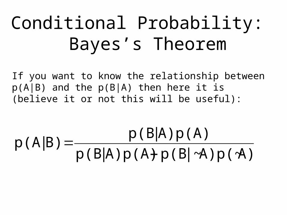
Conditional Probability: Bayes’s Theorem

A)A)p(~|~p(BA)p(A)|p(B

A)p(A)|p(BB)|p(A

If you want to know the relationship between p(A|B) and the p(B|A) then here it is (believe it or not this will be useful):

Probability and the Normal Distribution

If we know that 21% of a population (a proportion of 0.21) is left-handed, and we randomly sample one person from that population, what is the probability that we will sample someone who is left-handed? p=0.21 of course.

– Keep that in mind...

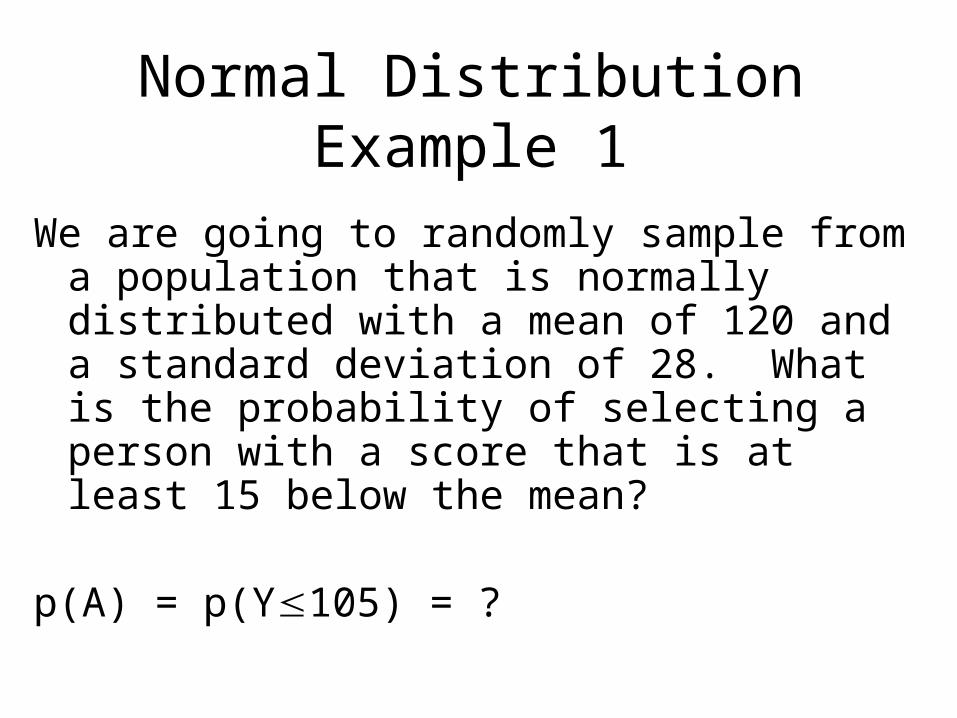
Normal Distribution Example 1

We are going to randomly sample from a population that is normally distributed with a mean of 120 and a standard deviation of 28. What is the probability of selecting a person with a score that is at least 15 below the mean?

p(A) = p(Y105) = ?

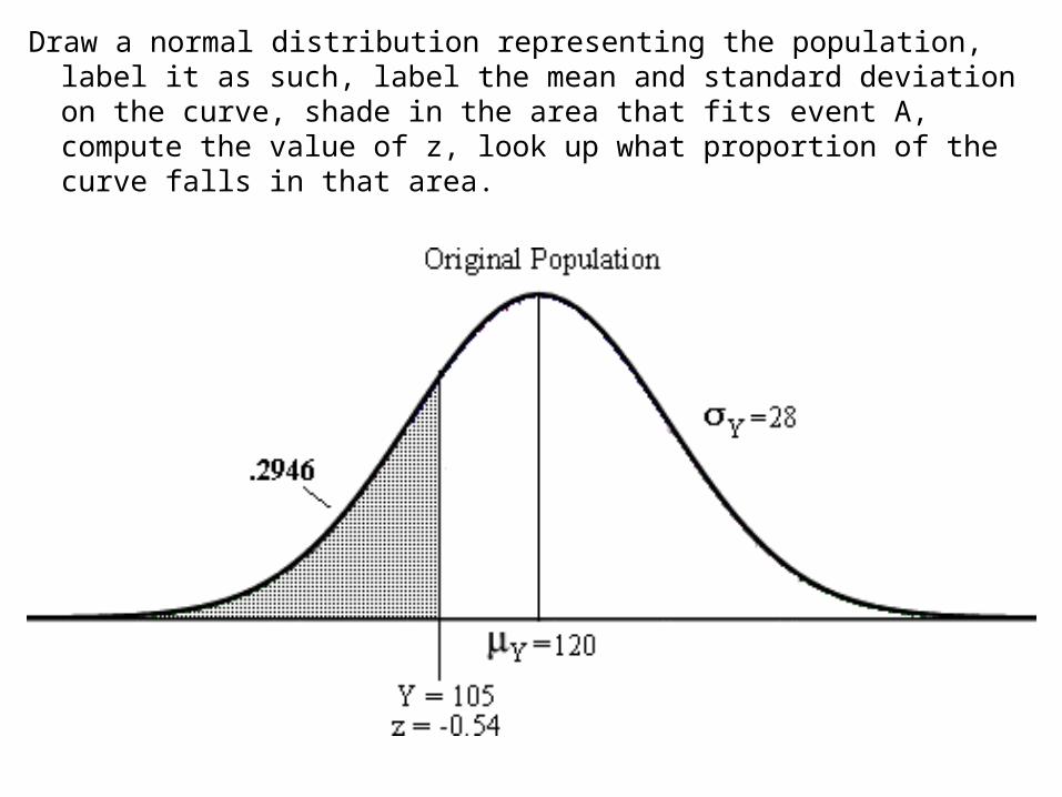
Draw a normal distribution representing the population, label it as such, label the mean and standard deviation on the curve, shade in the area that fits event A, compute the value of z, look up what proportion of the curve falls in that area.

Probability

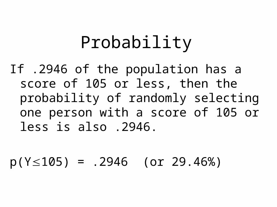
If .2946 of the population has a score of 105 or less, then the probability of randomly selecting one person with a score of 105 or less is also .2946.

p(Y105) = .2946 (or 29.46%)

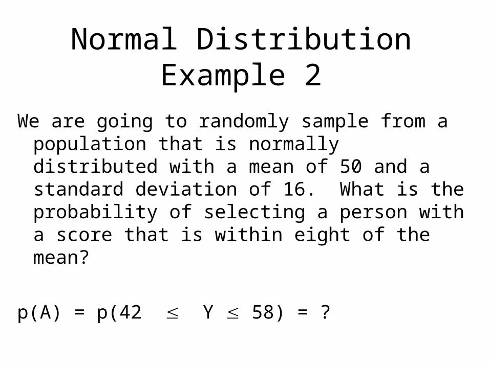
Normal Distribution Example 2

We are going to randomly sample from a population that is normally distributed with a mean of 50 and a standard deviation of 16. What is the probability of selecting a person with a score that is within eight of the mean?

p(A) = p(42 Y 58) = ?

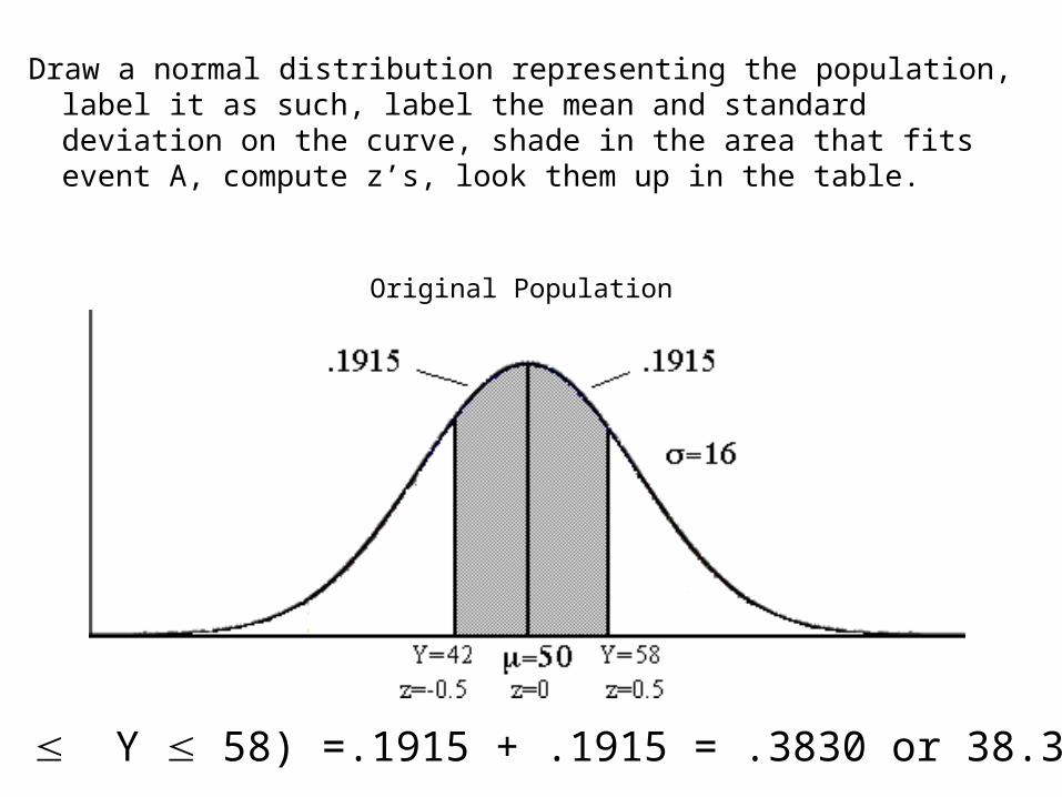
Draw a normal distribution representing the population, label it as such, label the mean and standard deviation on the curve, shade in the area that fits event A, compute z’s, look them up in the table.

Original Population

p(42 Y 58) =.1915 + .1915 = .3830 or 38.30%

One-tailed and two-tailed p values

We are going to want to ask questions that go in the opposite direction. For example, what value of z cuts off .05 (i.e. 5%) of the upper side of the curve (i.e. the value of z that there is a 5% chance of equaling or exceeding). The probabilities we are going to be the most interested in are .05 and the .01

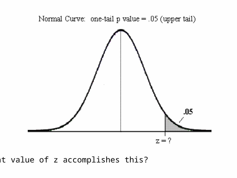
What value of z accomplishes this?

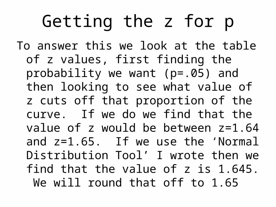
Getting the z for pTo answer this we look at the table of z

values, first finding the probability we want (p=.05) and then looking to see what value of z cuts off that proportion of the curve. If we do we find that the value of z would be between z=1.64 and z=1.65. If we use the ‘Normal Distribution Tool’ I wrote then we find that the value of z is 1.645. We will round that off to 1.65

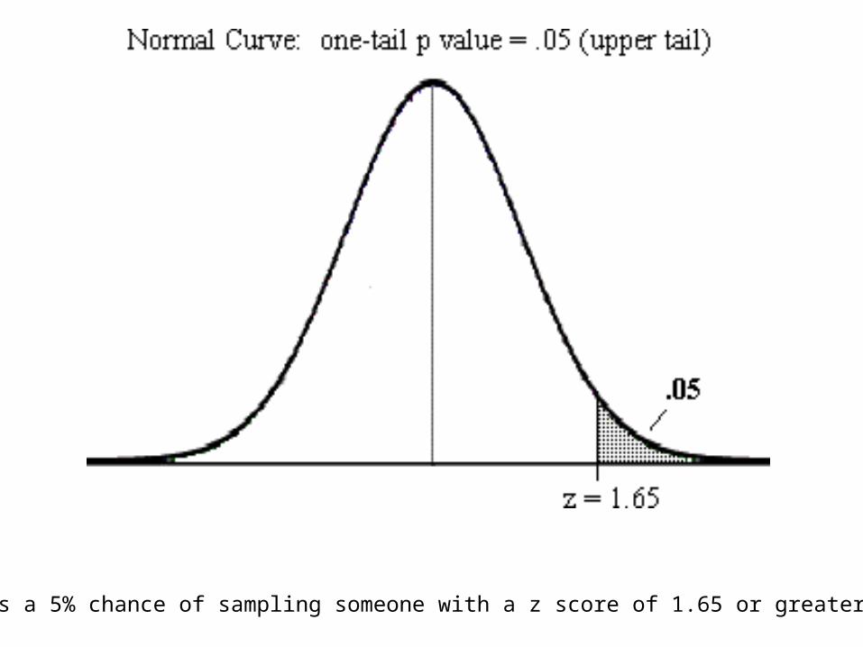
There is a 5% chance of sampling someone with a z score of 1.65 or greater

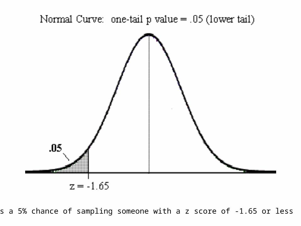
There is a 5% chance of sampling someone with a z score of -1.65 or less

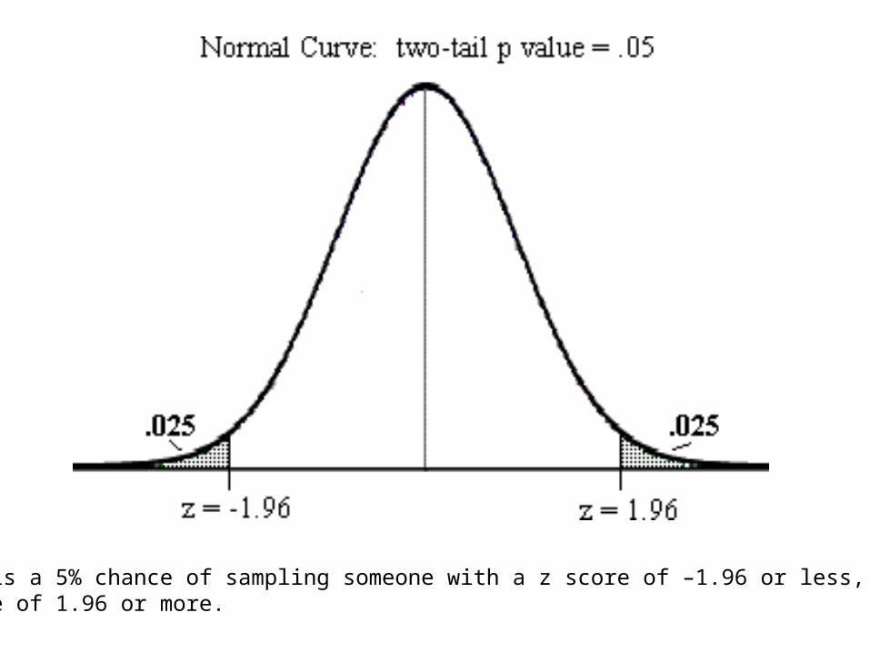
There is a 5% chance of sampling someone with a z score of –1.96 or less, or az score of 1.96 or more.

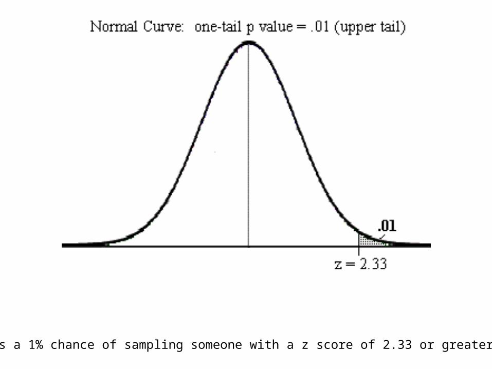
There is a 1% chance of sampling someone with a z score of 2.33 or greater

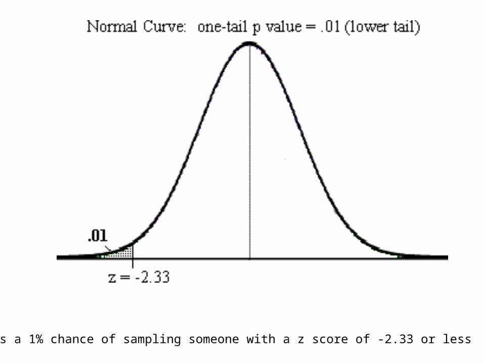
There is a 1% chance of sampling someone with a z score of -2.33 or less

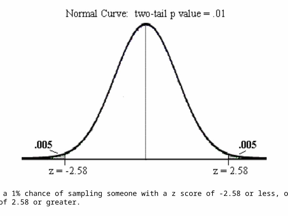
There is a 1% chance of sampling someone with a z score of -2.58 or less, or a z score of 2.58 or greater.