Provided by the author(s) and University College Dublin Library in accordance with publisher

policies., Please cite the published version when available.

Title New evidence on balanced growth, stochastic trends, and economic fluctuations

Authors(s) Whelan, Karl

Publication date 2004-10

Series Central Bank of Ireland Research Technical Paper; 7/RT/04

Publisher 2004 Copyright Central Bank of Ireland

Link to online version http://www.centralbank.ie/data/TechPaperFiles/7RT04.pdf

Item record/more information http://hdl.handle.net/10197/218

Downloaded 2019-03-09T19:40:17Z

The UCD community has made this article openly available. Please share how this access

benefits you. Your story matters! (@ucd_oa)

Some rights reserved. For more information, please see the item record link above.

7/RT/04 October 2004

CENTRAL BANK AND FINANCIAL

SERVICES AUTHORITY OF IRELAND

Research Technical Paper

New Evidence on Balanced Growth,

Stochastic Trends, and Economic Fluctuations

by

Karl Whelan∗

Economic Analysis and Research Department

P.O. Box 559, Dame Street

Dublin 2

Ireland

∗The views expressed in this paper are the personal responsibility of the author. They are not

necessarily held either by the Central Bank and Financial Services Authority of Ireland or the ESCB.

Email:karl.whelan@centralbank.ie.

Abstract

The one-sector Solow-Ramsey growth model informs how most modern researchers

characterize macroeconomic trends and cycles, and evidence supporting the model’s

balanced growth predictions is often cited. This paper shows, however, that the inclu-

sion of recent data leads to the balanced growth predictions being rejected. An alter-

native balanced growth hypothesis—that the ratio of nominal consumption to nominal

investment is stationary—is put forward, and new measures of the stochastic trends

and cycles in aggregate US data are derived based on this hypothesis. The contrasting

behavior of real and nominal ratios is consistent with a two-sector model of economic

growth, with separate production technologies for consumption and investment and two

stochastic trends underlying the long-run behavior of all macroeconomic series. Empir-

ical estimates of these stochastic trends are presented based on a structural VAR and

the role played in the business cycle by shocks to these trends is discussed.

1 Introduction

The one-sector Solow-Ramsey growth model remains the workhorse underlying a vast

amount of macroeconomic research. In particular, its “balanced-growth” prediction that

the ratios of real consumption, investment, and output should all be stationary (and thus

that the logs of the level series share a common stochastic trend) has played a key role

in modern macroeconomics. Sample averages of these “great ratios” are regularly used to

calibrate the long-run properties of a wide range of theoretical macroeconomic models. In

addition, the common trend prediction has played an important role in modern empirical

characterizations of macroeconomic trends and cycles. To cite a few well-known examples,

King, Plosser, Stock, and Watson (1991) have developed empirical methods to identify

a time series for this common trend, while Cochrane (1994) and Rotemberg and Wood-

ford (1996) have relied on the stationarity of the ratio of real consumption to real output

to provide econometric estimates of the transitory cyclical components of consumption,

investment, and output.

This paper presents new evidence on the traditional balanced growth hypothesis and on

the role of stochastic trends in the determination of U.S. macroeconomic fluctuations. The

evidence underlying the one-sector growth model is reconsidered and rejected, an alternative

balanced growth hypothesis consistent with a two-sector framework is suggested, and the

implications of this framework for macroeconomic trends and fluctuations are considered.

The contents of the paper are as follows. First, it is demonstrated that the inclusion of

recent data produces test results that point strongly against the balanced growth hypoth-

esis. For example, King, Plosser, Stock and Watson’s evidence for the hypothesis is still

widely cited. However, the sample in their study ends in 1988; using data through 2003,

the traditional balanced growth hypothesis turns out to be firmly rejected. Underlying

this rejection is the fact that the ratio of real investment to real consumption has moved

substantially upwards over time and now displays no evidence of mean-reversion.

Importantly, these results have been derived using standard National Income and Prod-

uct Accounts (NIPA) data. This implies a crucial distinction between these the formal

statistical tests presented here and the more informal evidence presented in the well-known

paper by Greenwood, Hercowitz, and Krusell (1997), who argue in favor of a model in which

real equipment investment rises relative to real GDP, but in which the real equipment se-

ries is defined using Robert Gordon’s (1990) alternative price index. That the balanced

growth property is clearly rejected for NIPA data has important implications that go well

1

beyond those discussed by Greenwood et al because NIPA data form the basis for the vast

majority of empirical work on US macroeconomics, and much of this work relies explictly

or implicitly on the balanced growth hypothesis.

Second, the paper discusses the implications of the failure of the traditional balanced

growth hypothesis for the measurement of stochastic trends and cycles. It is shown that

the estimated Vector Error Correction Model (VECM) implied by the traditional one-

sector balanced growth hypothesis produces unintuitive trending estimates of the cyclical

components of consumption, investment and output. Because these results contradict much

of the received wisdom on this issue that was outlined in previous papers based on NIPA

data such as those cited above, the paper is careful to illustrate how the incorporation of

new data and revisions to historical data have contributed to overturning patterns that

were previously considered to be stylized facts.

Third, an alternative “balanced growth” hypothesis is put forward, which is that the

ratio of nominal investment to nominal consumption is stationary and evidence is pre-

sented that this hypothesis is consistent with US macroeconomic data. This nominal-ratio

balanced growth hypothesis implies that the logs of real consumption, real investment, and

the relative price of consumption to investment can together be characterized according to

a VECM with a single cointegrating vector. Using this alternative VECM, new measures of

the transitory components of aggregate consumption, investment, and output are developed

and the implications of these alternative measures for the interpretation of recent business

cycles are explored.

Fourth, a simple structural model is proposed that is compatible with the long-run

properties of the data and the model’s implications are explored. The differing behavior

over time of the real and nominal ratios of consumption and investment are, by definition,

due a decline over time in the price of investment relative to the price of consumption, a

pattern that cannot occur in the one-sector growth model. However, this pattern is con-

sistent with a two-sector model of economic growth in which separate technological trends

in the consumption and investment sectors drive the relative price of output in the two

sectors. In addition, the existence of a single cointegrating vector among consumption,

investment, and their relative price implies a common trends representations in which the

long-run behavior of these variables depends on two separate I(1) stochastic trends. Using

a simple two-sector model, a set of long-run restrictions are derived that allow for the use

of the King, Plosser, Stock, Watson (1991) methodology to identify these stochastic trends

2

as corresponding to the states of technology in the consumption- and investment-producing

sectors. The dynamic responses to the two types of technology shocks are discussed, as

are the roles played by these shocks in generating business cycle fluctuations. It is con-

cluded that technology shocks play a limited role in generating business cycle fluctuations

in consumption, investment, and output.

Finally, the structural VAR implied by the two-sector model is extended to incorporate

hours worked, and the effect of the two types of technology shocks on hours are explored.

Results show that both types of technology shocks—for consumption- and investment-

producing sectors—tend to produce declines in hours worked on impact, a result that

confirms and extends the previous findings in a one-sector context of Galı (1999).

2 Tests of the Traditional Balanced Growth Hypothesis

The starting point for the standard neoclassical growth model is an aggregate resource

constraint of the form Ct + It = Yt = AtF (Kt, Lt) where the production function displays

diminishing marginal returns productivity with respect to capital accumulation. It is also

usually assumed that a representative consumer maximizes the present discounted value

of utility from real consumption, subject to a law of motion for capital and a process for

aggregate technology. If the technology process grows at a constant long-run average rate,

then it is well known that the model’s solution features all real variables, C, I,K, and Y ,

growing at the same average rate in the long-run. Thus, ratios of any of the real aggregates

will be stationary stochastic processes.

The intuition for this property of the one-sector growth model is very general and it

holds across a wide range of specifications for preferences and technology. Given diminishing

marginal returns to capital accumulation, a once-off increase in the savings rate can only

allow capital to grow faster than output for a temporary period, and a trend in the savings

rate will not be optimal for any standard specification of preferences.1 Thus, ratios involving

any of the variables capital, investment, consumption and output must be stationary.

Beyond theory, the hypothesis of stationary “great ratios” has been held as a crucial styl-

ized fact in macroeconomics at least as far back as the well-known contributions of Kaldor

(1957) and Kosobud and Klein (1961). More recently, King, Plosser, Stock, and Watson

1See, for instance the discussion of capital-output ratio dynamics in the Solow Model in Chapter 4 of

DeLong (2002)

3

(1991, henceforth KPSW), using NIPA data through 1988, presented formal econometric

evidence for the balanced growth hypothesis using modern time-series methods. KPSW’s

results are still widely cited as important evidence for the one-sector model’s long-run re-

strictions. However, Figure 1(a) shows that the traditional balanced growth predictions

appear empirically invalid once we use updated NIPA data. The figure shows the ratio

of real private fixed investment to real consumption expenditures (the same measures of

investment and consumption used in KPSW’s study). That this ratio should be stable is

the essence of the balanced growth hypothesis: The model’s other long-run restrictions—

such as the stationarity of the ratio of real consumption to aggregate real output or of real

investment to aggregate real output—will follow directly from stationarity of the ratio of

consumption to investment.2

Figure 1(a) shows that the ratio of real investment to real consumption has moved

upwards substantially over time and shows little apparent tendency for mean-reversion.

Importantly, most of the increase in this ratio occurred after 1988, the last year in KPSW’s

sample. Also notable is the fact that, despite the substantial slump in investment during

the recession beginning in 2001, this ratio is still at a historically very high level even in the

final period shown, 2003:Q2. Table 1 shows that formal statistical evidence confirms the

absence of mean reversion suggested by the chart. Panel A reports results from three tests

of the null hypothesis that the ratio series contains a unit root. The first is the standard

Augmented Dickey-Fuller t-test; the second is the DF GLS test of Elliot, Rothenberg and

Stock (1996) which has superior power to the ADF test; the third is the MZGLSα test of

Ng and Perron (2001) which has been shown to have excellent size and power properties.

For each test, the lag lengths for the test regressions was chosen using Ng and Perron’s

Modified AIC procedure. In all three cases, the tests do not come close to rejecting the

unit root hypothesis at conventional levels of significance.

The table also reports some more direct hypothesis tests of the balanced growth hypoth-

esis. In general, the null hypothesis of no cointegration between the log of real investment

and the log of real consumption can be rejected. However, normalizing the coefficient

2This statement implicitly follows the model in defining real output as an aggregate of consumption and

fixed investment. In contrast, KPSW tested for stationarity of the ratio of real consumption to real private

GDP (real GDP excluding government purchases). This differs from an aggregate of consumption and fixed

investment when net exports and inventory investment are non-zero. The preference here for the simpler

output measure is due to its consistency with the pure one-sector growth model, but the results in this

section are not overturned by instead looking at ratios involving private GDP. See Section 3.4 below.

4

on real investment to be one, one can reject the hypothesis that the coefficients on con-

sumption in the estimated long-run relationship is minus one, as implied by the one-sector

model’s balanced growth hypothesis. Panel B’s point estimate of -0.853 is derived from

the Stock-Watson dynamic least-squares estimation methodology and the balanced growth

hypothesis that this coefficient is minus one is tested using an asymptotically valid t-test.3.

Panel C’s point estimate of -0.851 is derived from the maximum likelihood systems estima-

tion methodology of Søren Johansen (1995), while its test of the balanced growth hypothesis

is based on a Wald test statistic derived from comparison of the log-likelihoods for the con-

strained and unconstrained systems (this has an asymptotic χ21 distribution.) In both cases,

the traditional balanced growth hypothesis is rejected at significantly greater than the one

percent level.

The fact that the null hypothesis of cointegration between the logs of consumption and

investment still cannot be rejected implies that, technically, one cannot reject the idea that

there still exists a single-common-trend representation for these two series. However, it

is hard to imagine what the economic basis for such a single trend representation would

be. For example, in an economy with a single technology process, why would a unit shock

to that process result in a one-percent increase in investment but only a 0.85 percent

increase in consumption. And why would this long-run relationship always have to take

the form (1,−0.85)? The one-sector growth model provides a powerful intuition about the

convergent forces that make it unsustainable for the levels of consumption and investment to

have different long-run trends. This provides a theoretical case for (1,−1) as a cointegrating

vector that is completely absent for the vector (1,−0.85) or any other vector (1,−b) where

b does not equal one.4

Figure 1(b) provides an alternative way to think about balanced growth and long-run

relationships. The figure shows the ratio of nominal private fixed investment to nominal

consumption. Unlike the ratio of the real series, this ratio exhibits no apparent trend over

time. Table 2 confirms that this alternative notion of balanced growth—that the ratio of

nominal expenditures on the two categories is stable over time—receives strong empirical

support from the same statistical tests that rejected the traditional formulation of balanced

3The exact procedure followed here is discussed on pages 608-612 of Hamilton (1994).4This is not to say that one cannot find empirical models based on this alternative notion of balanced

growth. For example, Kim and Piger (2002) use the one-sector growth model to motivate a single common

trend for consumption, investment, and output, and then implement this idea by equating log-consumption

with the trend and allowing for non-unit weights on the trend for log-investment and log-output.

5

growth. Panel A reports that the hypothesis that the nominal ratio contains a unit root

is firmly rejected by each of our tests, while Panels B and C show that point estimates of

the cointegrating vectors for the logs of the nominal series are very close to (1,−1), and

statistical tests cannot come close to rejecting this null hypothesis.

A first (somewhat obvious) observation about this alternative formulation of balanced

growth is that the difference between the series in Figures 1(a) and 1(b) is in itself evidence

against the one-sector growth model. The model’s assumption that consumption and invest-

ment goods are produced using the same technology implies that any decentralized market

equilibrium must feature them having the same price, and so real ratios and nominal ratios

should be the same thing. The differences between the two charts reflect different price

developments for the types of goods: Specifically, it reflects a substantial decline over time

in the ratio of investment prices to consumption prices. This relative price movement likely

reflects the existence of different production technologies for consumption and investment.

Once one allows for the idea that consumption and investment can be produced using

different technologies, and thus that their prices do not always move together, then the sta-

bility of the nominal ratio of investment to consumption also provides an intuitive version of

the same “sustainability” idea that underlies the one-sector model’s balanced growth pre-

diction. In the one-sector context, the ratio of real investment to real consumption cannot

trend upwards over time because households will not wish to allocate ever higher-fractions

of their incomes towards saving. However, in a two-sector model with faster technologi-

cal progress in the production of investment goods, then real investment can grow faster

than real consumption without requiring ever-increasing sacrifices on the part of house-

holds. Moreover, the original intuition behind the one-sector balanced growth hypothesis

still holds as an explanation for why the nominal ratio of investment to consumption should

be stationary: Increases in the household savings rate (the fraction of nominal income that

is saved) will only provide a temporary boost to the growth rates of capital and output.

3 Implications for Measurement of Trends and Cycles

The empirical properties just documented suggest that the appropriate theoretical frame-

work for thinking about long-run restrictions on US macro data is one with two types of

production technology (thus allowing investment and consumption prices to be different)

and with balanced growth formulated in terms of stability of the nominal ratio. We will

outline such a model, and how to identify the two technology shocks and their dynamic

6

effects, in Sections 4 and 5.

First, however, we will present some implications of the competing balanced growth

hypotheses that hold independent of any specific theoretical framework used to derive them.

Specifically, the long-run cointegrating restrictions implied by these hypotheses provide a

natural way to decompose macroeconomic time series into a stochastic trend component

on the one hand, and a transitory cyclical component on the other. We show here that

the traditional one-sector balanced growth hypothesis produces unsatisfactory estimates of

the cyclical components in consumption, investment, and output, and these estimates are

compared with those based on the alternative nominal ratio hypothesis.

3.1 Traditional Balanced Growth Method

According to the Granger representation theorem, the traditional formulation of the bal-

anced growth hypothesis—that log real investment it and log real consumption, ct are

cointegrated with a (1,-1) cointegrating vector—implies the existence of a VECM represen-

tation of the following type:

∆ct

∆it

=

αc

αi

+B(L)

∆ct−1

∆it−1

+

γi

γc

(it−1 − ct−1) + εt. (1)

The results from the estimation of a two-lag version of this VECM are reported in Table 3.5

The coefficients on the error-correction term (the investment-consumption ratio) are both

negative, with the coefficient in the investment regression being larger. This implies that

a high value of the real investment to real consumption ratio is a negative signal for future

growth in both consumption and investment, and that the ratio should tend to decline by

a process of investment falling by more than consumption. However, while these coefficient

estimates technically imply a stable VAR, it should be kept in mind that both cointegration

tests and unit root tests on the investment-consumption ratio reject the hypothesis that

this is a satisfactory model of investment and consumption dynamics.

This VECM can be used to derive a Beveridge-Nelson-style decomposition of consump-

tion and investment into their stochastic trend and transitory cycle components. Letting ω

and ψ represent the unconditional expectations for ∆ct and it − ct, the terms in the VECM

5This two-lag version is consistent with results from lag-length selection tests which favor three lags in

the levels specification.

7

can be re-arranged to arrive at a VAR representation in ∆ct − ω and it − ct − ψ:

(I − C(L))

∆ct − ω

it − ct − ψ

= εt. (2)

This can be written in companion matrix form as

Zt = AZt−1 + εt. (3)

Our definition of the transitory cyclical component of consumption is

ccyct = lim

k→∞

Et (ct − ct+k + kω) . (4)

In other words, the cyclical component is the expected cumulative shortfall in future con-

sumption growth relative to its trend growth rate, so that when this component is positive,

one should expect the average future growth rate of consumption to be below its trend rate.

This can be estimated from the VAR as

ccyct = −e′1

(

A+A2 +A3 + ....)

Zt = −e′1A (I −A)−1 Zt (5)

where e1 is a (1, 0) vector. The cyclical component of investment can also be estimated

from this VAR as

icyct = lim

k→∞

Et (it − it+k + kω)

= limk→∞

Et (it − ct + ct − ct+k + ct+k − it+k + kω)

= ccyct + (it − ct − ψ) (6)

Figure 2(a) shows the transitory components of investment and consumption generated

by the VECM reported in Table 3. Both series display the unsatisfactory property of

appearing to trend upwards over time, with the values early in the sample tending to be

negative and the values later in the sample tending to be positive.6 This feature is more

evident for investment than for consumption: The non-stationarity is due to both series

placing some weight on the real investment-consumption ratio, and the VECM coefficients

suggest that this is a more important signal for future investment growth than for future

consumption growth.

6It should be noted that the general pattern reported here turns out to be robust to the addition of a

wide range of other cyclical variables to the forecasting VAR.

8

3.2 Nominal Ratio Method

The same technique can be used to derive the transitory components implied by the

nominal-ratio balanced growth hypothesis. In this case, the VECM is formulated as

∆ct

∆it

∆pt

=

αc

αi

αp

+B(L)

∆ct−1

∆it−1

∆pt−1

+

γi

γc

γp

(it−1 − pt−1 − ct−1) + εt. (7)

where pt is the log of the price of consumption relative to the price of investment. The results

from the estimation of a two-lag version of this VECM are reported in Table 4. As with

the real-ratio system, the coefficients on the error-correction term (in this case the nominal

investment-consumption ratio) are both negative, with the coefficient in the investment

regression being larger. However, the sizes of the adjustment coefficients are larger and

more statistically significant. In addition, the unit root and cointegration tests suggest

that this system provides an acceptable model of the joint dynamics of real investment,

real consumption and their relative price.

Letting ωc, ωi, and µ represent the unconditional expectations of consumption growth,

investment growth and the nominal ratio of investment to consumption, the nominal-ratio

system implies a VAR representation of the form:

(I − C(L))

∆ct − ωc

∆it − ωi

it − pt − ct − µ

= εt. (8)

Again, writing this system in the same companion matrix format as equation (3), the

cyclical components of consumption and investment can be measured as

ccyct = −e′1A (I −A)−1 Zt (9)

icyct = −e′2A (I −A)−1 Zt (10)

where ei is a vector with one as its ith component and zeros elsewhere.

Figure 2(b) shows these new measures of the cyclical components of consumption and in-

vestment. As with the measures based on the real-ratio VECM, the nominal-ratio approach

implies that the cyclical component of investment is generally larger and more volatile than

the cyclical component of consumption. However, unlike the real ratio approach, these

measures do not trend over upwards over time.

9

3.3 Measures of the Aggregate Cycle

Figure 3 presents measures of the cyclical component of aggregate output generated by the

two alternative VECMs. These measures have been defined as

ycyc = θccyc + (1 − θ)icyc (11)

where θ is the sample average of the ratio of nominal consumption to the sum of nomi-

nal consumption and nominal investment. This measure is consistent with the concept of

aggregate real output as a Divisia index of consumption and investment, which is essen-

tially identical to the Fisher chain-index methodology that has been used to construct real

aggregates in the US NIPAs since 1996.7

Beyond the fact that the cyclical series implied by the real ratio method trends upwards,

while the nominal-ratio-based measure does not, the most striking aspect of Figure 3 is the

substantially different stories these series tell about the cyclical behavior of output since the

early 1990s. The real ratio model sees the long expansion of the 1990s as having brought

the economy way above its stochastic trend, with output a massive 13 percent above trend

at its peak in 2000:Q2. And this model views the recent economic downturn as only having

partially reversed this pattern, with output still being 7 percent above its trend level in

2003:Q2.

In contrast, the nominal ratio model sees the recession of the early 1990s as having

being particularly severe in the sense of bringing output farthest below its stochastic trend.

This model thus sees the long, largely investment-led, expansion of the 1990s as mainly an

unwinding of this development. The series generated by the nominal ratio model is also in

keeping with the common perception of the post-2000 period as one of cyclical weakness,

with the economy seen as 5 percent below its stochastic trend in 2003:Q2.

3.4 Comparison with Previous Results

The results just presented may be somewhat surprising because they seem to contradict the

findings of a number of well-known papers that have used the restriction of stationary real

7In light of the evidence of a declining relative price of investment, this measure is clearly superior to the

Laspeyeres or fixed-weight approach, which amounts to using the “real shares” implied by a particular base

year to weight the growth rates. The level of such a real investment share will be higher the farther back in

time is the base year, and for any fixed base year, this share will trend updwards over time, implying that

real output growth would tend to asymptote over time to simply equal the growth rate of real investment.

See Jones (2002) and Whelan (2002) for a discussion of these issues.

10

ratios to generate apparently satisfactory business cycle measures. This section highlights

two of these papers, one by John Cochrane (1994) and the other by Julio Rotemberg and

Michael Woodford (1996), and illustrates how the different conclusions reached here reflect

mainly the effect of a longer sample and data revisions.

Cochrane (1994): This paper examined the ratio of real consumption of nondurables and

services to real GDP and presented evidence in favor of its stationarity. Cochrane concluded

that a useful measure of the temporary component of output could be constructed from

the VECM implied by this cointegrating relationship. How can Cochrane’s conclusions be

reconciled with our earlier results, which showed the ratio of real consumption to real fixed

investment declining over time? The explanation has two parts.

The first relates to Cochrane’s use of a ratio involving total real GDP. Figure 4 shows

that the ratio studied by Cochrane has been relatively stable over time, and has fluctuated

within a narrow band. However, when one uses private GDP—consistent with our approach

of only looking at private consumption and investment—a downward trend becomes evident,

as implied by our earlier results. This interpretation is backed up by formal hypothesis tests

which indicate stationarity of the ratio featuring total GDP and non-stationarity of the ratio

featuring private GDP, both for the full sample and for the sample ending in 1989:Q3, as

in Cochrane’s paper.

Figure 5(a) shows the differences between the Beveridge-Nelson measures of the cyclical

component of output that emerge from these two alternative potential “cointegrating”

VARs, i.e. one featuring the ratio involving total real GDP and the other featuring private

real GDP. Consistent with our earlier results, the cyclical measure based on the private

GDP ratio is unsatisfactory because it trends upwards over time. In contrast, the cyclical

measure based on total real GDP does appear to be stationary.

How does one interpret the stationarity of the ratio involving total real GDP? Clearly,

in light of the evidence already presented, one cannot draw on the logic of the one-sector

model. Instead, the stationarity of this series appears to rest on a somewhat fortuitous

offset: Real government expenditures have declined relative to real GDP in a fashion that

has helped to mask the decline in real consumption relative to the rest of private GDP.

The second part of the explanation is that there have been important revisions to his-

torical data. Cochrane’s paper acknowledged that it may be preferable to employ a VAR

that uses the private GDP ratio, and he reports that for his data, this ratio appears station-

11

ary. Because our results for the same sample point towards this ratio being nonstationary,

it is clear that revisions to historical data have contributed to the different conclusions

reached here. Such revisions have included the introduction of hedonic price indexes for

various categories of investment goods, as well as other steps aimed at addressing some of

the issues raised about capital goods price indexes by researchers such as Robert Gordon

(1990). These revisions have had the effect of boosting the historical growth rates of real

investment relative to real consumption.

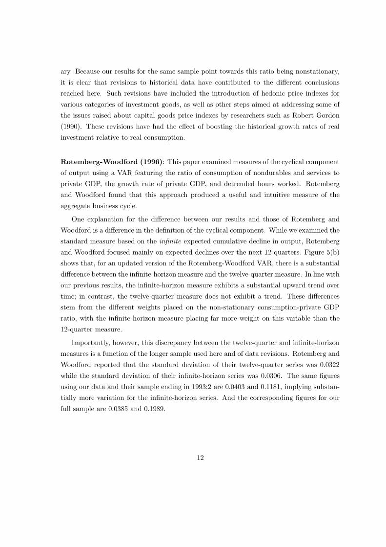
Rotemberg-Woodford (1996): This paper examined measures of the cyclical component

of output using a VAR featuring the ratio of consumption of nondurables and services to

private GDP, the growth rate of private GDP, and detrended hours worked. Rotemberg

and Woodford found that this approach produced a useful and intuitive measure of the

aggregate business cycle.

One explanation for the difference between our results and those of Rotemberg and

Woodford is a difference in the definition of the cyclical component. While we examined the

standard measure based on the infinite expected cumulative decline in output, Rotemberg

and Woodford focused mainly on expected declines over the next 12 quarters. Figure 5(b)

shows that, for an updated version of the Rotemberg-Woodford VAR, there is a substantial

difference between the infinite-horizon measure and the twelve-quarter measure. In line with

our previous results, the infinite-horizon measure exhibits a substantial upward trend over

time; in contrast, the twelve-quarter measure does not exhibit a trend. These differences

stem from the different weights placed on the non-stationary consumption-private GDP

ratio, with the infinite horizon measure placing far more weight on this variable than the

12-quarter measure.

Importantly, however, this discrepancy between the twelve-quarter and infinite-horizon

measures is a function of the longer sample used here and of data revisions. Rotemberg and

Woodford reported that the standard deviation of their twelve-quarter series was 0.0322

while the standard deviation of their infinite-horizon series was 0.0306. The same figures

using our data and their sample ending in 1993:2 are 0.0403 and 0.1181, implying substan-

tially more variation for the infinite-horizon series. And the corresponding figures for our

full sample are 0.0385 and 0.1989.

12

4 A Simple Two-Sector Model

We have described the econometric implications of our alternative nominal ratio formulation

of balanced growth. Here, we provide a simple two-sector model that provides a theoretical

foundation for this approach, and document some additional implications of the model for

the long-run behavior of consumption, investment, and their relative price.

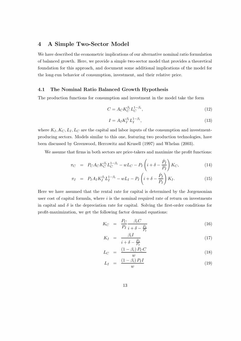
4.1 The Nominal Ratio Balanced Growth Hypothesis

The production functions for consumption and investment in the model take the form

C = ACKβc

C L1−βc

C , (12)

I = AIKβi

I L1−βi

I , (13)

where KI ,KC , LI , LC are the capital and labor inputs of the consumption and investment-

producing sectors. Models similar to this one, featuring two production technologies, have

been discussed by Greenwood, Hercowitz and Krusell (1997) and Whelan (2003).

We assume that firms in both sectors are price-takers and maximize the profit functions:

πC = PCACKβc

C L1−βc

C − wLC − PI

(

i+ δ −PI

PI

)

KC , (14)

πI = PIAIKβi

I L1−βi

I −wLI − PI

(

i+ δ −PI

PI

)

KI . (15)

Here we have assumed that the rental rate for capital is determined by the Jorgensonian

user cost of capital formula, where i is the nominal required rate of return on investments

in capital and δ is the depreciation rate for capital. Solving the first-order conditions for

profit-maximization, we get the following factor demand equations:

KC =PC

PI

βcC

i+ δ − PI

PI

(16)

KI =βiI

i+ δ − PI

PI

(17)

LC =(1 − βc)PCC

w(18)

LI =(1 − βi)PII

w(19)

13

An implication of these conditions is that for both factors, the ratios of the quantities of

the factor used in the two sectors are strictly proportional to the ratio of nominal outputs:

KI

KC

=βi

βc

PII

PCC, (20)

LI

LC

=1 − βi

1 − βc

PII

PCC. (21)

Now consider the properties of this economy along a steady-state growth path, that is

a growth path in which all real variables in the economy grow at constant rates. Note first

that if capital in the j sector is growing at a constant rate Gj , then investment in that type

of capital must be given by

Ij = (Gj + δ)Kj (22)

Thus, the composition of output in the investment sector along a steady-state growth path

can be written as

I =PC

PI

βc (GC + δ)C

i+ δ − PI

PI

+βi (GI + δ) I

i+ δ − PI

PI

(23)

This re-arranges to givePII

PCC=

βc (GC + δ)

i+ δ − PI

PI− βi (GI + δ)

(24)

Because the quantity on the right can be assumed to be constant along a steady-state

growth path, the ratio of nominal outputs is also constant.

If we move away from deterministic steady-states, and instead assume that the tech-

nology shocks for consumption and technology sectors evolve in a stochastic fashion with

trend growth rates µI and µC , i.e. that

∆aC,t = µC + ηC,t (25)

∆aI,t = µI + ηI,t (26)

where ηC,t and ηI,t are I(0) series, then for a wide range of standard specifications for prefer-

ences, the economy’s dynamic stochastic general equilibrium will feature the growth rates of

consumption, investment, and relative prices all equalling their nonstochastic steady-state

values plus a set of stationary deviations. Thus, these results provide a simple theoretical

basis for our alternative formulation of long-run balanced growth.

Before moving on, it should be noted of course that the assumption of Cobb-Douglas

technology—and most specifically its implication of unit-elastic factor demands—is essen-

tial to the derivation of the result of a stable long-run nominal ratio of consumption to

14

investment. While some may feel uncomfortable with this restrictive specification of the

production technology, the model has been designed to fit the evidence on the stability of

this nominal ratio and unit-elastic factor demands, and hence Cobb-Douglas technology,

appear to be necessary to fit this pattern. In addition, it may be worth noting that the

recent work of Jones (2004) demonstrates that Cobb-Douglas-shaped aggregate production

functions can be derived from ideas-based models under very general assumptions.

4.2 Other Long-Run Restrictions

In addition to providing an economic basis for the nominal ratio balanced growth hypoth-

esis, the two-sector model implies a clear set of restrictions on the joint long-run behavior

of consumption, investment, and their relative price. To see this, note that equations (20)

and (22) together imply that, along the steady-state growth path, IC and II—and thus KC

and KI—must expand at the same growth rate as aggregate real investment.

Normalizing the steady-state growth rate of aggregate labor input to zero (implying

constant labor input in both sectors) and denoting the steady-state growth rates of the

consumption- and investment-sector technologies by µC and µI , these considerations imply

that the steady-state growth rates of consumption and investment are determined by:

gC = µC + βcgI (27)

gI = µI + βigI (28)

These equations solve to give

gC = µC +βcµI

1 − βi

(29)

gI =µI

1 − βi

(30)

The real growth rates of consumption and investment will generally differ along the steady-

state growth path, with investment growing faster as long as µI > µC .

The fact that the ratio of nominal outputs of the two sectors is constant along the

steady-state growth path implies that the growth rate of the price of consumption relative

to the price of investment will be the negative of the relative growth rates of the quantities,

i.e. that

gP = gI − gC =

(

1 − βc

1 − βi

)

µI − µC (31)

15

We will now discuss how the long-run restrictions implied by the two-sector model allow

us to identify the stochastic processes for consumption- and investment-sector technology

as well as the dynamic effects of shocks to these technologies.

5 Identifying Two Technology Shocks

5.1 The VMA Representation

We have described how our preferred nominal-ratio balanced growth hypothesis implied

two different representations, the VECM system of equation (7), and the VAR system

of equation (8). In addition, however, it is well known that any cointegrated VAR with

n variables and r cointegrating relations can also be represented using a Vector Moving

Average (VMA) representation of the form

∆Xt = θ +D (L) εt, (32)

where D(1) has a reduced rank of n − r reflecting the restrictions on long-run behavior

imposed by the cointegrating relations. In the case of the nominal ratio model, this means

the existence of a representation of the form

∆Xt =

∆ct

∆it

∆pt

= θ +D (L) εt. (33)

where D(1) has a rank of two.

A reduced-form VMA representation can be derived directly from inverting the VECM

representation and this can be used to derive impulse responses to the shock terms εt. How-

ever, the shock terms and impulse responses obtained from this reduced-form representation

are not unique. For any nonsingular matrix G, there exists an observably equivalent repre-

sentation of the form

∆Xt = θ +(

D (L)G−1)

Gεt, (34)

with shock terms Gεt and impulse responses given by D (L)G−1. So, to obtain shocks

and impulse responses that have a useful economic interpretation, it is necessary to impose

theory-based restrictions on the G matrix.

In the rest of this section, we show how the long-run restrictions implied by our two-

sector model can be combined with the method of King, Plosser, Stock and Watson (1991)

16

to identify structural shocks and impulse responses that are consistent with this model. In

other words, we identify a structural representation

∆Xt = θ + Γ (L) ηt (35)

in which the shocks ηt have an economic interpretation consistent with our model.

5.2 Identification Methodology

The identification of the structural representations proceeds in a number of steps. The first

step is to note that any system of n different I(1) variables with r cointegrating relationships

can be expressed in terms of the Stock and Watson (1988) common trends representation

with n − r common trends. This means that the non-stationary I(1) components of our

three variables can be expressed as functions of two I(1) stochastic trends. Algebraically,

these so-called “permanent” components can be written as

Xpt = X0 +Aτt (36)

τt = µt+t∑

s=1

ηps (37)

where A is a 3 × 2 matrix, ηpt is a vector containing the two shocks to the permanent

component, and Aµ = θ.

The second step notes that our two-sector model provides the restrictions to allow us

to identify the two common trends as corresponding to the states of technology in the

consumption- and investment-producing sectors. This allows one to write the matrix of

long-run effects in the structural VMA represention as

Γ (1) =(

A 0)

(38)

with the vector of shocks being written as

ηt =

ηpt

ηtt

(39)

where ηtt represents the model’s sole transitory shock.

Third, the model pins down the A matrix. Together, equations (29), (30), and (31)

imply that the long-run multipliers can be written as

Γ (1) =

1 βc

1−βi0

0 1

1−βi0

−1 1−βc

1−βi0

(40)

17

where the first two columns describe the long-run effects of the consumption technology

shock and the investment technology shock respectively.

This information is sufficient to identify the two technology shocks from the reduced-

form VMA. This is done as follows. Starting from the definition of the structural shocks,

we have

Γ (1) ηt = D (1) εt. (41)

Multiplying both sides by Γ′ (1), this becomes

Γ′ (1) Γ (1) ηt = Γ′ (1)D (1) εt. (42)

This can be re-written as

A′A 0

0 0

ηpt

ηtt

=

A′D (1)

0

εt. (43)

So, the technology shocks are identified as

ηpt =

(

A′A)−1

A′D (1) εt. (44)

The transitory shock can be identified from the assumption that it is uncorrelated with

either of the technology shocks. This implies a unique (up to a scalar multiple) 1 × 3

vector of coefficients that describes the linear combination of the reduced-form shocks that

is orthogonal to both of the structural shocks. Specifically, letting Ω be the covariance

matrix of the reduced-form errors, εt, and defining[

(A′A)−1A′D (1)

]

⊥to be a 3× 1 vector

such that(

A′A)−1

A′D (1)[

(

A′A)−1

A′D (1)]

⊥= 0 (45)

then the transitory shock is defined as

ηtt =

[

(

A′A)−1

A′D (1)]′

⊥Ω−1εt. (46)

In terms of the notation used in equation (34), the long-run restriction methodology achieves

identification by setting

G =

(A′A)−1A′D (1)

[

(A′A)−1A′D (1)

]′

⊥Ω−1

(47)

The generality of this identification methodology is worth noting: It relies only on the

long-run restrictions implied by the two-sector growth model and on the assumption that

18

the technology shocks are uncorrelated with the transitory shock. Importantly, no assump-

tion whatsoever has been made about the covariance structure of the technology shocks

themselves. As we will discuss below, this is an important advantage of this methodology.

Finally, note that this identification of the structural shocks allows for a direct economic

interpretation of the Beveridge-Nelson decompositions presented earlier. This is because,

by definition, the expected values of deviations in the distant future from the variables’

permanent components—defined in equations (36) and (37)—are all zero, so these are

identical to the permanent components identified by our Beveridge-Nelson decompositions

in Section 2. And the economic interpretation of the transitory components produced by

these decompositions is that they represent the components of consumption, investment,

and output that are unrelated to the states of technology in either the consumption- or

investment-producing sectors.

5.3 Results

In the analysis that follows, the standard value of the capital elasticity of one-third was

applied to both sectors, i.e βi = βc = 1

3is used. This is based on evidence relating to the

composition of value-added by industry which suggest that sectors oriented towards the

production of capital goods appear to have similar capital shares to the rest of the sectors.8

With these assumptions, our long-run identifying restrictions become

Γ (1) =

1 0.5 0

0 1.5 0

−1 1 0

. (48)

It should be noted, however, that the pattern of the results reported here remain quite

similar when a range of different plausible values are used for βc and βi.

The empirical implementation of the two-sector identification was carried out using a

three-variable cointegrated VAR featuring the log of per capita real consumption, the log

of per capita real fixed investment, and the log of the relative price of consumption to

investment.9 As before, the sample was 1949:1 to 2003:2 and the system was estimated

with three lags.10

8Greenwood, Hercowitz and Krusell (1997) also argue that this is a reasonable assumption.9The population measure used is the civilian population aged sixteen and over.

10This is the lag length consistent with the optimal value for the Akaike Information Criterion; however,

the substance of the results discussed here were not found to be sensitive to the lag length chosen.

19

We first consider the technology shocks that emerge from the imposition of the model’s

long-run restrictions. Figure 6(a) displays the estimates of the two technology series, aC,t

and aI,t. Not surprisingly, in light of the facts documented earlier, the series for investment

technology has grown faster over the whole sample than the series for consumption technol-

ogy. However, what may be somewhat more surprising is that this pattern only becomes

evident after 1980. The reasons for this can be seen in Figure 6(b). The gap between the

two technology series can be equated with the long-run component of the price of consump-

tion relative to investment. The figure shows that the transitory component for the relative

price series is quite small, and that the series appeared to be relatively stationary up until

about 1980, after which it increased steadily.

Our empirical estimates of the average growth rates of the stochastic trends (µC and

µI) allow us to calculate—via equation (29)—the average contributions of the two types of

technological progress to the steady-state growth in consumption per capita. The average

growth rate of consumption technology, µC , is estimated to be 0.31 percent per quarter,

while µI is estimated at 0.45 percent per quarter. These parameters are estimated fairly

tightly: Standard errors based on 5000 bootstrap replications of the reduced-form VAR

process are 0.04 percent for µC and 0.06 percent for µI . Using these figures along with

our assumption of βc = βi = 1

3, equation (29) implies that 42 percent of long-run growth

in consumption per capita is due to technological improvements in the investment sector,

with the rest being due to technological progress in the consumption sector. And using a

long-run ratio of nominal consumption to nominal investment of 4:1, these figures imply

that technological progress in the investment sector accounts for 54 percent of long-run

growth in a Divisia index of output per capita.

Turning from long-run trends to the behavior of the observed series relative to their

estimated permanent components, an important pattern that emerges from Figures 2(b)

and 6(b) is that consumption and relative prices tend to stay much closer to their permanent

components than does investment. This result, of course, echoes the conclusions of Fama

(1992), Cochrane (1994), and others that transitory shocks play a much smaller role in

determining consumption than they do in determining investment. However, whereas these

and subsequent researchers have viewed this result as implying that consumption is a useful

proxy for a unique single common trend that also underlies investment and output, in our

case, this pattern simply means that consumption stays close to a weighted average of two

different stochastic trends, one due to consumption technology and one due to investment

20

technology.

Figure 7 illustrates the impulse responses of consumption, investment, and their relative

price to shocks to the consumption and investment technologies as well as to the model’s

single transitory shock. These impulse responses help to flesh out why it is that investment

deviates more substantially than the other variables from its permanent component (see

Figure 2(b)). First, they show that investment is substantially more responsive to the

transitory shock than the other variables, both in the magnitude of its maximum response

and the time it takes for the shock to wear off. Second, in the short-run, investment displays

large reactions to technology shocks that differ significantly from its long-run responses. For

instance, although consumption technology has no effect on investment in the long run, the

short-run response of investment to a consumption technology shock is almost as positive

as the response of consumption. More intriguingly, the initial response of investment to

shocks to investment-sector technology is negative, with the response only moving towards

its long-run positive value with a substantial lag.

Finally, another way to understand the role of the various shocks is to calculate forecast-

error variance decompositions. As noted above, our long-run restrictions achieved identifi-

cation without imposing the assumption that the two technology shocks were uncorrelated.

Indeed, our estimated technology shocks have a positive correlation coefficient of 0.31.

While this is a useful property of our identification methodology—there is no good theo-

retical reason to impose the assumption of uncorrelated technology shocks in this case—it

does imply that the fraction of the variance assigned to each of the technology shocks will

depend arbitrarily on the ordering of the Cholesky decomposition that generates these re-

sults. In contrast, because the transitory shock is assumed to be orthogonal to each of the

permanent shocks, the fraction of error variance due to this shock is independent of any

ordering of the permanent shocks in the decomposition. For this reason, we restrict our

focus to the role played by the transitory shock. These results are reported on Table 5,

which in addition to the variance decompositions for c, i, and p also adds a column denoted

y which reports the variance decomposition for the Divisia measure of output.

Two results stand out from Table 5. The first is the contrast between the role played

by transitory shocks in determining consumption and relative prices when compared with

investment. At the medium-run frequency of twelve quarters, transitory shocks determine

38 percent of the error variance for consumption and only 4 percent for relative prices;

these percentages then decline steadily as the forecast horizon is lengthened. In contrast,

21

transitory shocks appear to dominate the short-run variance of investment, and while their

relative importance declines with the forecast horizon, they still determine 60 percent of

the error variance for investment at a horizon of 50 quarters.

More generally, because investment fluctuations contribute disproportionately to ag-

gregate business cycle fluctuations, the results show a very substantial role for transitory

shocks in determining cyclical fluctuations in real output. For example, transitory shocks

determine 68 percent of the error variance for output at a horizon of 12 quarters. Over-

all, these results confirm and extend the conclusions of King, Plosser, Stock, and Watson

(1988) that transitory, non-technology-related shocks appear to play an important role in

determining business cycle fluctuations, with the effects of these shocks being most notable

for investment.

5.4 On “Investment-Specific” Technology Shocks

Following Greenwood, Hercowitz, and Krusell (1997), some researchers have described the

technology terms in two-sector models such as ours using a slightly different formulation.

This formulation would see our model re-written as

C = zKβc

C L1−βc

C , (49)

I = zqKβi

I L1−βi

I , (50)

with z termed “neutral” technology and q termed “investment-specific” technology. As a

theoretical matter, this formulation provides an isomorphic description of the economy to

ours. In terms of identifying the technology series, the z series is identical to our consump-

tion technology series while the log of the q series is the difference between the logs of our

investment technology and consumption technology series. Similarly, our analysis of the

effects of technology shocks can be re-phrased in terms of this alternative formulation: The

impulse response to a neutral shock that produces a unit increase in the technology series

for both sectors can be calculated simply by adding together the impulse responses for the

two technology shocks in our analysis. And the effects of a so-called investment-specific

shock—a shock that improves investment technology but not consumption technology—are

identical to the effects of the investment-sector shock that we have described.

However, beyond its usage as an alternative way of describing of the model, this for-

mulation does have empirical content if it is assumed that the shocks to the z and q series

are uncorrelated, as is done for instance in Greenwood, Hercowitz, Krusell (2000). This

22

assumption implies that, ceteris paribus, one should expect that any positive shock to

consumption technology should also show up one-for-one in the technology of the invest-

ment sector. Our analysis allowed for identification of consumption- and investment-sector

technology shocks without any assumptions about their covariance, and the results based

upon this more general identification call into doubt the idea of uncorrelated neutral and

investment-specific shocks.

Specifically, in our analysis, investment-specific technology shocks can be calculated as

the difference between investment-sector shocks and consumption-sector shocks. Thus cal-

culated, there is a statistically significant negative correlation between investment-specific

shocks and consumption (i.e. neutral) shocks of -0.34. One way of explaining this result

is to note that the correlation between technology shocks in the two sectors, while posi-

tive, is weak enough that a positive shock to consumption technology tends to imply that

consumption technology increases relative to investment technology, (implying a decline in

measured investment-specific technology). These calculations place in doubt the accuracy

of identifications that rely on the assumption of uncorrelated z and q shocks.

6 Technology Shocks and Hours

One potential weakness of the structural VAR system just analyzed is that it failed to

consider the role played by labor market variables in economic fluctuations. Labor input

was acknowledged only by expressing consumption and investment in per capita terms. By

neglecting the effect of technology shocks on hours worked, it is possible that there is some

bias in the previous results on the medium-run effects of technology shocks on consumption

and investment.

Another reason to extend the model to incoporate variations in hours is that the effect of

technology shocks on labor input has itself been the subject of an important debate in recent

years. In particular, Jordi Galı (1999) has shown that technology shocks appear to have a

negative impact effect on hours worked, which stands in stark contrast to the predictions of

the standard real business cycle model. Galı’s results are implicitly based on a one-sector

model, in that they describe the effect of a single economy-wide technology shock, which is

identified as the sole determinant of aggregate labor productivity in the long-run. Here, we

briefly describe how our methodology can be used to identify the separate effects on hours

worked of shocks to consumption- and investment-producing technologies.

23

The approach taken here is to re-apply our analysis replacing per capita consumption

and investment with consumption-per-hour and investment-per-hour, and then to add hours

to the structural VAR. As in Galı (1999), nonfarm business hours are used as the labor

input measure and the nonstationarity of this series is dealt with by characterizing it as

being I(1).

The structural identification of the previous section is extended here by assuming that

technology shocks have no long-run effects on hours, and that the non-stationarity of hours

is driven by a single I(1) permanent component. In other words, the identification is

implemented via a four-variable restricted VMA in (∆ct,∆it,∆pt,∆ht), where the Γ (1)

matrix of equation (40) becomes

Γ (1) =

1 βc

1−βi0 0

0 1

1−βi0 0

−1 1−βc

1−βi0 0

0 0 1 0

(51)

This re-formulation of the model turns out to imply very little change from our earlier

results on the effects of technology shocks on consumption, investment, and relative prices.

Thus, these results are not repeated. However, the results for the effect of technology

shocks on hours are worth showing. Figure 8 reports that, for both types of technology

shocks, the impact effects on hours worked are negative. The chart also shows the 10th and

90th percentiles from the bootstrap distribution based on 5000 replications of the estimated

reduced-form VAR process. In each case, the upper 90th percentiles corresponding to the

impact periods are negative, indicating that the finding of a negative impact response

appears to be statistically significant. These results thus provide some support for Galı’s

arguments against models in which positive technology shocks induce immediate increases

in labor input.

24

7 Conclusions

This paper has had a number of goals.

First, it has been shown that the inclusion of recent data from the US national accounts

overturns earlier widely-cited results that supported the one-sector model’s balanced growth

predictions. This is important because the idea of stable “great ratios” of real consumption

to real investment or of real investment to real GDP, has generally been considered a central

stylized fact in macroeconomics. The fact that real investment appears to have a different

long-run trend growth rate from real consumption in US data should have important im-

plications for macroeconomic analysis, given that many empirical and theoretical studies

take the one-sector growth model as a baseline for characterizing the long-run behavior of

the economy.

Second, an alternative formulation of the idea of balanced growth—that the ratio of

nominal consumption to nominal investment should be stationary—was suggested and

found to provide a good description of the US data. It was shown that this formulation

produces estimates of the transitory or cyclical components of consumption and invest-

ment that have more satisfactory features than those based on the traditional “real ratio”

formulation of balanced growth.

Third, a simple two-sector framework was proposed that is consistent with the long-run

properties of the data. The model acknowledges that capital goods appear to be produced

with a different technology than consumption goods, with the pace of technological change

in the production of capital goods being faster on average. A structural VAR analysis was

implemented to explore the implications of this approach for the macroeconomic effects of

technology shocks. The results suggest that technology shocks are not a dominant force

driving the business cycle, and that the response of labor input to these shocks is at odds

with the predictions of the standard real business cycle model. In light of these results,

an obvious next direction for research is the development of theoretical models that are

consistent with the long-run facts presented here and are also consistent with the evidence

concerning the role played in business cycles by technology shocks.

25

References

[1] Cochrane, John (1994). “Permanent and Transitory Components of GNP and Stock

Prices.” Quarterly Journal of Economics, 109, 241-265.

[2] DeLong, J. Bradford (2002). Macroeconomics, McGraw-Hill.

[3] Elliot, Graham, Thomas Rothenberg and James Stock (1996). “Efficient Tests for an

Autoregressive Unit Root,” Econometrica, 64, 813-836.

[4] Fama, Eugene (1992). “Transitory Variation in Investment and Output,” Journal of

Monetary Economics, 30, 467-480.

[5] Galı, Jordi (1999). “Technology, Employment, and the Business Cycle: Do Technology

Shocks Explain Aggregate Fluctuations,” American Economic Review, 89, 249-271.

[6] Gordon, Robert J. (1990). The Measurement of Durable Goods Prices, Chicago: Uni-

versity of Chicago Press.

[7] Greenwood, Jeremy, Zvi Hercowitz, and Per Krussell (1997). “Long-Run Implications

of Investment-Specific Technological Change.” American Economic Review, 87, 342-

362.

[8] Greenwood, Jeremy, Zvi Hercowitz, and Per Krussell (2000). “ The Role of Investment-

Specific Technological Change in the Business Cycle, European Economic Review, 44,

91-115.

[9] Johansen, Søren (1995). Likelihood-Based Inference in Cointegrated Vector Auto-

Regressive Models, Oxford: Oxford University Press.

[10] Jones, Charles I. (2002). Using Chain-Weighted NIPA Data, Federal Reserve Bank of

San Francisco Economic Letter No. 2002-22.

[11] Jones, Charles I. (2004). The Shape of Production Functions and the Direction of

Technical Change, mimeo, University of California at Berkeley.

[12] Kaldor, Nicholas (1957). “A Model of Economic Growth.” Economic Journal, 67, 591-

624.

26

[13] Kim, Chang-Jin and Jeremy Piger (2002). “Common Stochastic Trends, Common

Cycles, and Asymmetry in Economic Fluctuations,” Journal of Monetary Economics,

49, 1189-1211.

[14] Kosobud, Robert and Lawrence Klein (1961). “Some Econometrics of Growth: Great

Ratios of Economics,” Quarterly Journal of Economics, 78, 173-198.

[15] King, Robert, Charles Plosser, James Stock, and Mark Watson (1991). “Stochastic

Trends and Economic Fluctuations.” American Economic Review, 81, 819-840.

[16] Ng, Serena and Pierre Perron (2001). “Lag Length Selection and the Construction of

Unit Root Tests with Good Size and Power,” Econometrica, 69, 1519-1554.

[17] Rotemberg, Julio and Michael Woodford (1996). “Real-Business-Cycle Models and the

Forecastable Movements in Output, Hours, and Consumption,” American Economic

Review, 86, 71-89.

[18] Whelan, Karl (2002). A Guide to U.S. Chain Aggregated NIPA Data, Review of Income

and Wealth, 48, 217-233.

[19] Whelan, Karl (2003). A Two-Sector Approach to Modeling U.S. NIPA Data, Journal

of Money, Credit, and Banking, 35, 627-656.

27

Table 1: Tests of the Traditional Balanced Growth Hypothesis

A. Unit Root Tests for ic

Test Statistic 5%/10% ValuesADF t-statistic -2.00 -2.88/-2.57Elliot-Rothenberg-Stock DFGLS -1.53 -1.95/-1.62Ng-Perron MZGLS

α -2.74 -8.10/-5.70

B. Estimated Cointegrating Vector: Stock-Watson DOLS

Variable Null Hypothesis Estimateslog (i) 1 1log (c) -1 -0.853

t-test of Balanced Growth Restriction: t = −4.39 (p=0.00001)

C. Estimated Cointegrating Vector: Maximum Likelihood

Variable Null Hypothesis Estimateslog (i) 1 1log (c) -1 -0.851

Wald Test of Balanced Growth Restriction: χ21 = 13.13 (p=0.0003)

Notes : i ≡ Real private fixed investment at 1996 dollars, c ≡ Real consumption expenditures at

1996 dollars. Sample is 1949:1 to 2003:2. DOLS estimation was based on four first-difference leads

and four lags; t-test calculated as in Hamilton (1994) pages 608-612. Lag length for ML VAR was

three (chosen by AIC). See text for additional details.

Table 2: Tests of the Nominal-Ratio Balanced Growth Hypothesis

A. Unit Root Tests for i∗

c∗

Test Statistic 5%/10% ValuesADF t-statistic -3.07 -2.88/-2.57Elliot-Rothenberg-Stock DFGLS -2.80 -1.95/-1.62Ng-Perron MZGLS

α -8.50 -8.10/-5.70

B. Estimated Cointegrating Vector: Stock-Watson DOLS

Variable Null Hypothesis Estimateslog (i∗) 1 1log (c∗) -1 -0.993

t-test of Balanced Growth Restriction: t = −0.222 (p=0.82)

C. Estimated Cointegrating Vector: Maximum Likelihood

Variable Null Hypothesis Estimateslog (i∗) 1 1log (c∗) -1 -1.006

Wald Test of Balanced Growth Restriction: χ21 = 0.32 (p=0.57)

Notes : i∗ ≡ Nominal private fixed investment, c∗ ≡ Nominal consumption expenditures. Sample

is 1949:1 to 2003:2. DOLS estimation was based on four first-difference leads and four lags; t-test

calculated as in Hamilton (1994) pages 608-612. Lag length for ML VAR was five (chosen by AIC).

See text for additional details.

Table 3: VECM Implied by Traditional Balanced Growth Hypothesis

∆ct ∆it

Constant -0.009 -0.053

(-1.074) (-2.283)

∆ct−1 -0.102 0.260

(-1.220) (1.126)

∆ct−2 0.253 0.400

(3.043) (1.745)

∆it−1 0.062 0.409

(2.044) (4.845)

∆it−2 -0.008 -0.016

(-0.294) (-0.202)

it−1 − ct−1 -0.008 -0.034

(1.563) (2.300)

Notes : i ≡ Real private fixed investment, c ≡ Real consumption expenditures. Sample is 1949:1 to

2003:2. t−statistics are given in parentheses below coefficient estimates

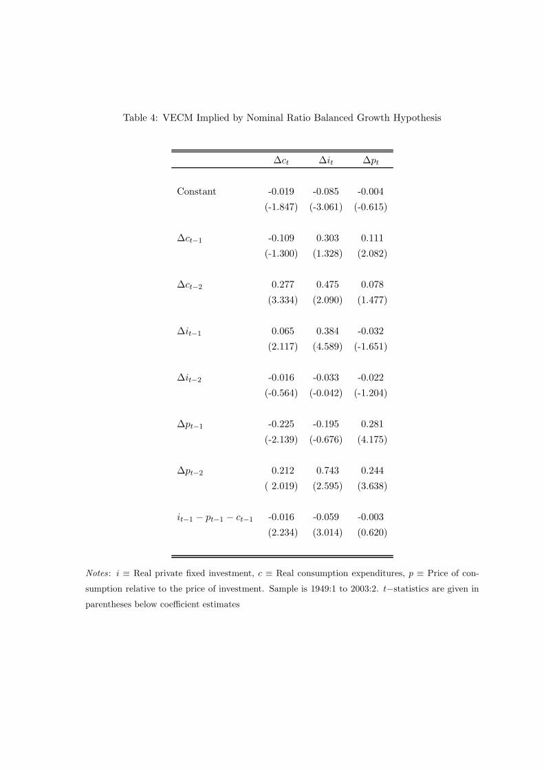
Table 4: VECM Implied by Nominal Ratio Balanced Growth Hypothesis

∆ct ∆it ∆pt

Constant -0.019 -0.085 -0.004

(-1.847) (-3.061) (-0.615)

∆ct−1 -0.109 0.303 0.111

(-1.300) (1.328) (2.082)

∆ct−2 0.277 0.475 0.078

(3.334) (2.090) (1.477)

∆it−1 0.065 0.384 -0.032

(2.117) (4.589) (-1.651)

∆it−2 -0.016 -0.033 -0.022

(-0.564) (-0.042) (-1.204)

∆pt−1 -0.225 -0.195 0.281

(-2.139) (-0.676) (4.175)

∆pt−2 0.212 0.743 0.244

( 2.019) (2.595) (3.638)

it−1 − pt−1 − ct−1 -0.016 -0.059 -0.003

(2.234) (3.014) (0.620)

Notes : i ≡ Real private fixed investment, c ≡ Real consumption expenditures, p ≡ Price of con-

sumption relative to the price of investment. Sample is 1949:1 to 2003:2. t−statistics are given in

parentheses below coefficient estimates

Table 5: Fraction of Forecast-Error Variance Due to Transitory Shocks

Horizon c i y pc

pi

1 0.496 0.881 0.794 0.113

(0.214) (0.145) (0.186) (0.127)

4 0.523 0.927 0.806 0.085

(0.210) (0.128) (0.180) (0.105)

8 0.463 0.940 0.754 0.053

(0.196) (0.124) (0.188) (0.076)

12 0.387 0.933 0.684 0.036

(0.169) (0.120) (0.181) (0.054)

16 0.321 0.908 0.610 0.027

(0.141) (0.117) (0.166) (0.040)

24 0.231 0.829 0.483 0.017

(0.100) (0.114) (0.135) (0.025)

40 0.144 0.675 0.330 0.009

(0.061) (0.111) (0.094) (0.013)

50 0.117 0.601 0.275 0.008

(0.049) (0.108) (0.079) (0.009)

Notes : Standard Errors Based on 5000 Bootstrap Replications in Parentheses. Sample is 1949:1 to

2003:2.

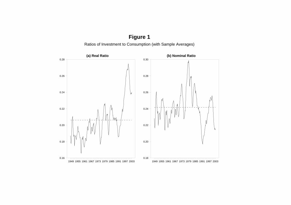
Figure 1Ratios of Investment to Consumption (with Sample Averages)

(a) Real Ratio

1949 1955 1961 1967 1973 1979 1985 1991 1997 20030.16

0.18

0.20

0.22

0.24

0.26

0.28(b) Nominal Ratio

1949 1955 1961 1967 1973 1979 1985 1991 1997 20030.18

0.20

0.22

0.24

0.26

0.28

0.30

Figure 2Cyclical Components from Real- and Nominal-Ratio-Based VECMs

Investment Consumption

(a) Real Ratio VECM

1949 1955 1961 1967 1973 1979 1985 1991 1997 2003-0.3

-0.2

-0.1

-0.0

0.1

0.2

0.3

0.4

Investment Consumption

(b) Nominal Ratio VECM

1949 1955 1961 1967 1973 1979 1985 1991 1997 2003-0.3

-0.2

-0.1

-0.0

0.1

0.2

0.3

Real Ratio Nominal Ratio

Figure 3Cyclical Component of Output from Real- and Nominal-Ratio-Based VECMs

1949 1953 1957 1961 1965 1969 1973 1977 1981 1985 1989 1993 1997 2001-0.10

-0.05

0.00

0.05

0.10

0.15

Total GDP Private GDP

Figure 4Ratios of Consumption of Nondurables and Services to Real GDP

1949 1953 1957 1961 1965 1969 1973 1977 1981 1985 1989 1993 1997 20010.55

0.60

0.65

0.70

0.75

0.80

0.85

0.90

Figure 5VAR-Based Measures of Expected Declines in Output

Private GDP Total GDP

(a) Cochrane VECM

1949 1955 1961 1967 1973 1979 1985 1991 1997 2003-0.100

-0.075

-0.050

-0.025

-0.000

0.025

0.050

0.075

0.100

Infinite Horizon Twelve Quarter Horizon

(b) Rotemberg-Woodford VAR

1949 1955 1961 1967 1973 1979 1985 1991 1997 2003-0.50

-0.25

0.00

0.25

0.50

Figure 6

Consumption Technology Investment Technology

Technology Series from Two-Sector SVAR

1949 1955 1961 1967 1973 1979 1985 1991 1997 20030.0

0.2

0.4

0.6

0.8

1.0

Data Permanent Component

Relative Price of Consumption

1949 1956 1963 1970 1977 1984 1991 1998-0.30

-0.25

-0.20

-0.15

-0.10

-0.05

-0.00

0.05

0.10

0.15

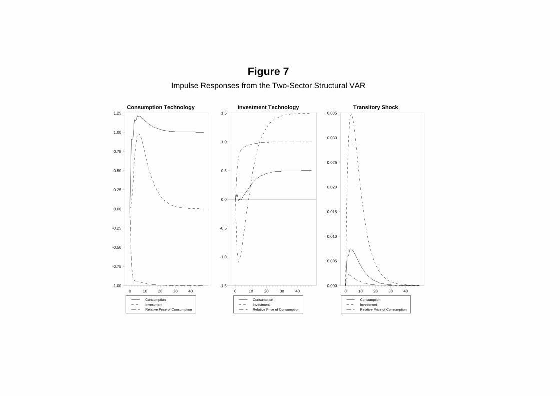
Figure 7Impulse Responses from the Two-Sector Structural VAR

ConsumptionInvestmentRelative Price of Consumption

Consumption Technology

0 10 20 30 40-1.00

-0.75

-0.50

-0.25

0.00

0.25

0.50

0.75

1.00

1.25

ConsumptionInvestmentRelative Price of Consumption

Investment Technology

0 10 20 30 40-1.5

-1.0

-0.5

0.0

0.5

1.0

1.5

ConsumptionInvestmentRelative Price of Consumption

Transitory Shock

0 10 20 30 400.000

0.005

0.010

0.015

0.020

0.025

0.030

0.035

Figure 8Response of Hours to Technology Shocks (With Bootstrapped 10% and 90% Fractiles)

Consumption Technology Shock

0 5 10 15 20 25 30 35-0.50

-0.25

0.00

0.25

0.50

0.75Investment Technology Shock

0 5 10 15 20 25 30 35-0.96

-0.80

-0.64

-0.48

-0.32

-0.16

0.00

0.16