Proton magnetic resonance spectroscopy in the brain: Report of

Proton magnetic resonance spectroscopy in the brain:Report of AAPM MR Task Group #9

Dick J. Drosta)

Nuclear Medicine and MRI Department, St. Joseph’s Health Centre, London, Ontario N6A 4L6, Canada

William R. RiddleDepartment of Radiology and Radiological Sciences, Vanderbilt University Medical Center,Nashville, Tennessee 37232-2675

Geoffrey D. ClarkeDepartment of Radiology, Division of Radiological Sciences, University of Texas Health Sciences Center,San Antonio, Texas 78284

~Received 28 January 2002; accepted for publication 14 June 2002; published 27 August 2002!

AAPM Magnetic Resonance Task Group #9 on proton magnetic resonance spectroscopy~MRS! inthe brain was formed to provide a reference document for acquiring and processing proton (1H)MRS acquired from brain tissue. MRS is becoming a common adjunct to magnetic resonanceimaging ~MRI!, especially for the differential diagnosis of tumors in the brain. Even though MRimaging is an offshoot of MR spectroscopy, clinical medical physicists familiar with MRI may notbe familiar with many of the common practical issues regarding MRS. Numerous research labora-tories performin vivo MRS on other magnetic nuclei, such as31P, 13C, and19F. However, mostcommercial MR scanners are generally only capable of spectroscopy using the signals from pro-tons. Therefore this paper is of limited scope, giving an overview of technical issues that areimportant to clinical proton MRS, discussing some common clinical MRS problems, and suggest-ing how they might be resolved. Some fundamental issues covered in this paper are common tomany forms of magnetic resonance spectroscopy and are written as an introduction for the reader tothese methods. These topics include shimming, eddy currents, spatial localization, solvent satura-tion, and post-processing methods. The document also provides an extensive review of the literatureto guide the practicing medical physicist to resources that may be useful for dealing with issues notcovered in the current article. ©2002 American Association of Physicists in Medicine.@DOI: 10.1118/1.1501822#

Key words: magnetic resonance spectroscopy, medical brain imaging, brain metabolism

TABLE OF CONTENTS

I. INTRODUCTION. . . . . . . . . . . . . . . . . . . . . . . . . . . .2178A. Larmor equation. . . . . . . . . . . . . . . . . . . . . . . . . .2178B. Magnetic resonance signal. . . . . . . . . . . . . . . . . . 2178C. Parts per million~ppm! scale. .. . . . . . . . . . . . . . 2178D. J coupling. . . . . . . . . . . . . . . . . . . . . . . . . . . . . . .2179E. Brain metabolites. . . . . . . . . . . . . . . . . . . . . . . . .2179F. Magnetic field homogeneity. . . . . . . . . . . . . . . . . 2180

II. TEST PHANTOM. . . . . . . . . . . . . . . . . . . . . . . . . . .2180III. SPECTROSCOPIC SEQUENCES. . . . . . . . . . . . . 2180

A. Point RESolved spectroscopy~PRESS!. . . . . . . 2181B. Stimulated echo acquisition mode~STEAM!. . . 2181C. PRESS and STEAM spectra. . . . . . . . . . . . . . . . 2181D. Chemical shift imaging. . . . . . . . . . . . . . . . . . . . 2182E. Single voxel vs chemical shift imaging. . . . . . . 2183

IV. SIGNAL-TO-NOISE RATIO. . . . . . . . . . . . . . . . . . 2183V. SHIMMING. . . . . . . . . . . . . . . . . . . . . . . . . . . . . . . .2184VI. EDDY CURRENTS. .. . . . . . . . . . . . . . . . . . . . . . .2185VII. PHASE CYCLING. . . . . . . . . . . . . . . . . . . . . . . . .2186VIII. PROBLEM WITH WATER. . . . . . . . . . . . . . . . . 2186IX. PROBLEM WITH LIPIDS. . .. . . . . . . . . . . . . . . . 2187

2177 Med. Phys. 29 „9…, September 2002 0094-2405 Õ2002Õ2

X. SELECTING SPECTROSCOPICPARAMETERS. . . . . . . . . . . . . . . . . . . . . . . . . . . . .2187

XI. PRESCAN ADJUSTMENTS. . . . . . . . . . . . . . . . . 2187XII. POST-PROCESSING. . . . . . . . . . . . . . . . . . . . . . .2188

A. Zero filling. . . . . . . . . . . . . . . . . . . . . . . . . . . . . .2189B. Apodization filter. . . . . . . . . . . . . . . . . . . . . . . . .2189C. Eddy current correction. . . . . . . . . . . . . . . . . . . . 2189D. Water-suppression filter. . . . . . . . . . . . . . . . . . . . 2189E. Fourier transform. . . . . . . . . . . . . . . . . . . . . . . . .2189F. Phasing. . . . . . . . . . . . . . . . . . . . . . . . . . . . . . . . .2190G. Baseline correction. . . . . . . . . . . . . . . . . . . . . . . .2192H. Peak areas. . . . . . . . . . . . . . . . . . . . . . . . . . . . . . .2192I. Correcting for relaxation and saturation. . . . . . . 2192J. Calculating concentrations. . . . . . . . . . . . . .. . . . 2193

XIII. MRS EQUIPMENT QUALITY CONTROL~QC!. . . . . . . . . . . . . . . . . . . . . . . . . . . . . . . . . . . .2193

XIV. COMMENTS FOR HIGH FIELDSPECTROSCOPY. . . . . . . . . . . . . . . . . . . . . . . . .2194

XV. MATHEMATICS USED INSPECTROSCOPY. . . . . . . . . . . . . . . . . . . . . . . . .2194

XVI. RECOMMENDATIONS AND SUGGESTEDREADING. . . . . . . . . . . . . . . . . . . . . . . . . . . . . . .2195

21779„9…Õ2177Õ21Õ$19.00 © 2002 Am. Assoc. Phys. Med.

op-c

leo

ines

onnfo

tehencrieonre

fesveeere

neu

oriledareonThlie-

th

toigh-

stilling

ec-he

pre-MRnce,ance

S-d is

em-nt in

or

cale

albylecies

is

de-em-

the

2178 Drost, Riddle, and Clarke: Report of AAPM MR Task Group #9 2178

I. INTRODUCTION

Proton magnetic resonance spectroscopy~MRS! is providedas an option by most manufacturers and is becoming mcommon in clinical practice, particularly for neurological aplications. Although MRS can be performed on nuclei suas 31P and13C, proton (1H) MRS requires only a softwarepackage plus a test phantom, making it the easiest andexpensive spectroscopy upgrade for the MRI system. Nproton spectroscopy requires radio frequency~RF! coilstuned to the Larmor frequency of other nuclei plus matchpreamplifiers, hybrids, and a broad-band power amplifiProton MRS software packages automate acquisitionquences and post-processing for metabolite quantificati1

However, the efficient implementation of MRS acquisitioprotocols is something that is beyond the expectationsmost MR technologists. Therefore, MR physicists are ofcalled in to perform MRS procedures to evaluate whetproblems with proton MRS are due to equipment malfutions, software problems, or operator errors. We give a boverview of clinical proton MRS, discuss some commclinical MRS problems, and suggest how they might besolved.

A. Larmor equation

In magnetic resonance, nuclei resonate at a frequency~f !given by the Larmor equation

f 5gB0 , ~1!

whereB0 is the strength of the external magnetic field andgis the nucleus’ gyromagnetic ratio. For protons,g is equal to42.58 MHz/Tesla. If all the proton nuclei in a mixture omolecules had the same Larmor frequency, magnetic rnance spectra would be limited to a single peak. Howethe magneticB0 field ‘‘seen’’ by a nucleus is shielded by thcovalent electron structure surrounding the nucleus. Thfore, nuclei with different chemical neighbors will havslightly different resonance frequencies~f ! given by

f 5gB0~12scs!, ~2!

where scs is a screening constant (uscsu!1). This smallchange in the resonance frequency is the basis for magresonance spectroscopy. Note that both the overall molecstructure and the proton~s! position within the molecule willdeterminescs or f.

B. Magnetic resonance signal

In spectroscopy, the strength of the MR signal is proptional to the number of protons at that frequency. Whspectroscopy can be described in the time domain, MRSare usually displayed in the frequency domain. In the fquency domain, the area under a specific peak is proportito the number of protons precessing at that frequency.frequency axis itself is reversed from ‘‘normal’’ for historicaprecedent. Before the introduction of the Fast FourTransform2 ~FFT! in 1965, almost all spectrometers employed continuous-wave irradiation, which swept eitherapplied magnetic field~an electromagnet! or the transmitter

Medical Physics, Vol. 29, No. 9, September 2002

re

h

astn-

gr.e-.

rnr-f

-

o-r,

e-

ticlar

-

ta-ale

r

e

frequency. The abscissa for spectra went from low fieldhigh field, which means that protons precessing at the hest frequencies would be recorded first~left-hand side!. Nowalmost all spectrometers use the FFT, but spectra aredisplayed historically with the abscissa displaying decreasfrequency from left to right.

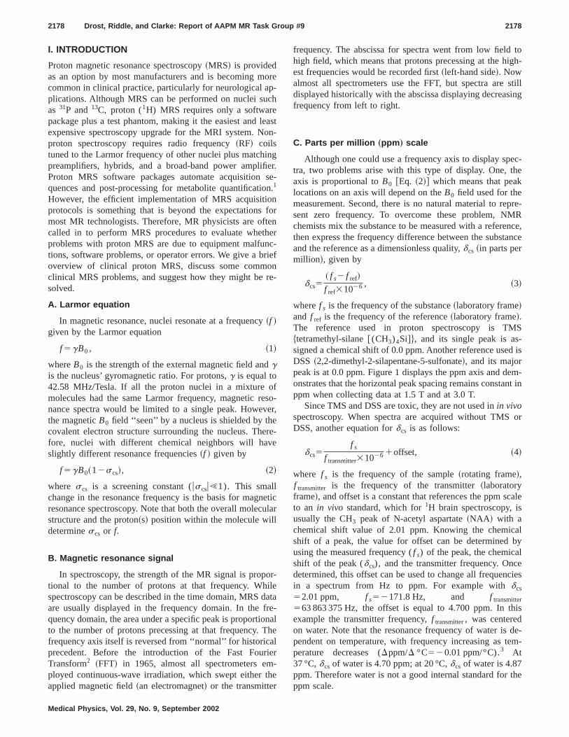
C. Parts per million „ppm … scale

Although one could use a frequency axis to display sptra, two problems arise with this type of display. One, taxis is proportional toB0 @Eq. ~2!# which means that peaklocations on an axis will depend on theB0 field used for themeasurement. Second, there is no natural material to resent zero frequency. To overcome these problem, Nchemists mix the substance to be measured with a referethen express the frequency difference between the substand the reference as a dimensionless quality,dcs ~in parts permillion!, given by

dcs5~ f s2 f ref!

f ref31026 , ~3!

wheref s is the frequency of the substance~laboratory frame!and f ref is the frequency of the reference~laboratory frame!.The reference used in proton spectroscopy is TM$tetramethyl-silane@(CH3)4Si#%, and its single peak is assigned a chemical shift of 0.0 ppm. Another reference useDSS ~2,2-dimethyl-2-silapentane-5-sulfonate!, and its majorpeak is at 0.0 ppm. Figure 1 displays the ppm axis and donstrates that the horizontal peak spacing remains constappm when collecting data at 1.5 T and at 3.0 T.

Since TMS and DSS are toxic, they are not used inin vivospectroscopy. When spectra are acquired without TMSDSS, another equation fordcs is as follows:

dcs5f s

f transmitter31026 1offset, ~4!

where f s is the frequency of the sample~rotating frame!,f transmitter is the frequency of the transmitter~laboratoryframe!, and offset is a constant that references the ppm sto an in vivo standard, which for1H brain spectroscopy, isusually the CH3 peak of N-acetyl aspartate~NAA ! with achemical shift value of 2.01 ppm. Knowing the chemicshift of a peak, the value for offset can be determinedusing the measured frequency (f s) of the peak, the chemicashift of the peak (dcs), and the transmitter frequency. Oncdetermined, this offset can be used to change all frequenin a spectrum from Hz to ppm. For example withdcs

52.01 ppm, f s52171.8 Hz, and f transmitter

563 863 375 Hz, the offset is equal to 4.700 ppm. In thexample the transmitter frequency,f transmitter, was centeredon water. Note that the resonance frequency of water ispendent on temperature, with frequency increasing as tperature decreases (Dppm/D °C520.01 ppm/°C).3 At37 °C,dcs of water is 4.70 ppm; at 20 °C,dcs of water is 4.87ppm. Therefore water is not a good internal standard forppm scale.


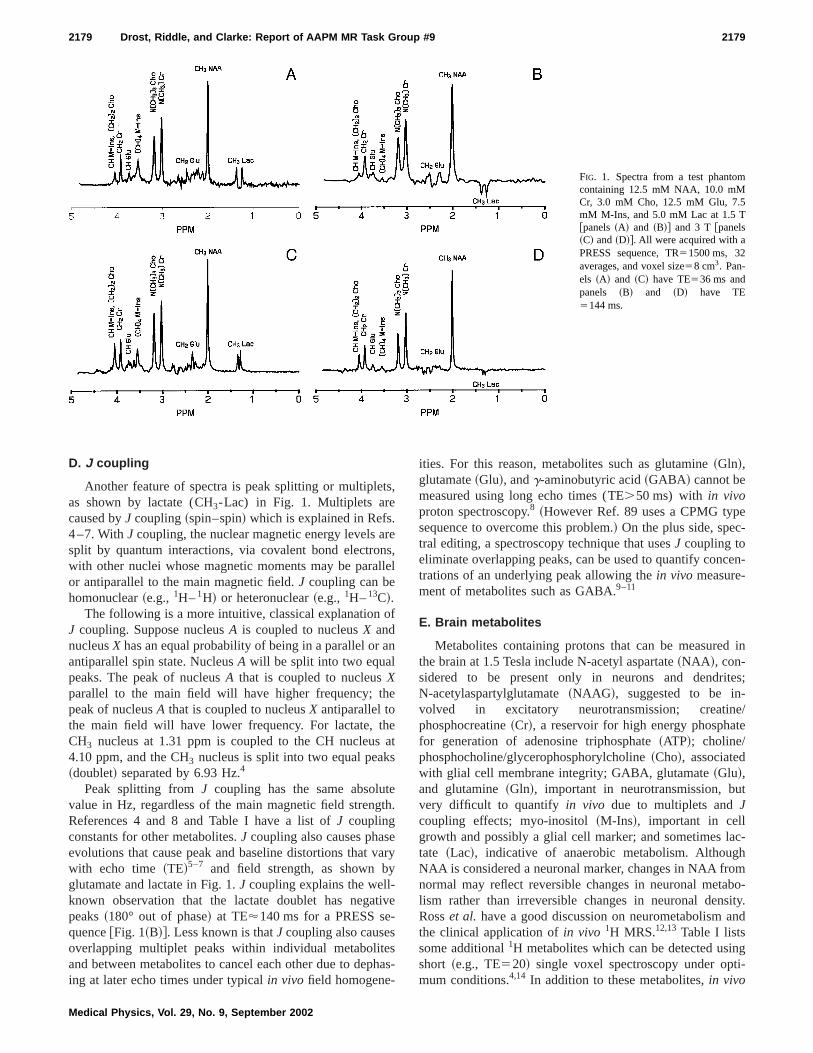
FIG. 1. Spectra from a test phantomcontaining 12.5 mM NAA, 10.0 mMCr, 3.0 mM Cho, 12.5 mM Glu, 7.5mM M-Ins, and 5.0 mM Lac at 1.5 T@panels~A! and ~B!# and 3 T @panels~C! and~D!#. All were acquired with aPRESS sequence, TR51500 ms, 32averages, and voxel size58 cm3. Pan-els ~A! and ~C! have TE536 ms andpanels ~B! and ~D! have TE5144 ms.

ts

.r

nsll

of

an

e

hea

s

teth

evay

tiv-ssh

e-

en-

in

tes;-e/te

t

ac-hmbo-ity.nd

ngi-

D. J coupling

Another feature of spectra is peak splitting or multipleas shown by lactate (CH3-Lac) in Fig. 1. Multiplets arecaused byJ coupling~spin–spin! which is explained in Refs4–7. WithJ coupling, the nuclear magnetic energy levels asplit by quantum interactions, via covalent bond electrowith other nuclei whose magnetic moments may be paraor antiparallel to the main magnetic field.J coupling can behomonuclear~e.g.,1H–1H! or heteronuclear~e.g.,1H–13C!.

The following is a more intuitive, classical explanationJ coupling. Suppose nucleusA is coupled to nucleusX andnucleusX has an equal probability of being in a parallel orantiparallel spin state. NucleusA will be split into two equalpeaks. The peak of nucleusA that is coupled to nucleusXparallel to the main field will have higher frequency; thpeak of nucleusA that is coupled to nucleusX antiparallel tothe main field will have lower frequency. For lactate, tCH3 nucleus at 1.31 ppm is coupled to the CH nucleus4.10 ppm, and the CH3 nucleus is split into two equal peak~doublet! separated by 6.93 Hz.4

Peak splitting fromJ coupling has the same absoluvalue in Hz, regardless of the main magnetic field strengReferences 4 and 8 and Table I have a list ofJ couplingconstants for other metabolites.J coupling also causes phasevolutions that cause peak and baseline distortions thatwith echo time ~TE!5–7 and field strength, as shown bglutamate and lactate in Fig. 1.J coupling explains the well-known observation that the lactate doublet has negapeaks~180° out of phase! at TE'140 ms for a PRESS sequence@Fig. 1~B!#. Less known is thatJ coupling also causeoverlapping multiplet peaks within individual metaboliteand between metabolites to cancel each other due to deping at later echo times under typicalin vivo field homogene-


,

e,

el

t

.

ry

e

as-

ities. For this reason, metabolites such as glutamine~Gln!,glutamate~Glu!, andg-aminobutyric acid~GABA! cannot bemeasured using long echo times (TE.50 ms) with in vivoproton spectroscopy.8 ~However Ref. 89 uses a CPMG typsequence to overcome this problem.! On the plus side, spectral editing, a spectroscopy technique that usesJ coupling toeliminate overlapping peaks, can be used to quantify conctrations of an underlying peak allowing thein vivo measure-ment of metabolites such as GABA.9–11

E. Brain metabolites

Metabolites containing protons that can be measuredthe brain at 1.5 Tesla include N-acetyl aspartate~NAA !, con-sidered to be present only in neurons and dendriN-acetylaspartylglutamate~NAAG!, suggested to be involved in excitatory neurotransmission; creatinphosphocreatine~Cr!, a reservoir for high energy phosphafor generation of adenosine triphosphate~ATP!; choline/phosphocholine/glycerophosphorylcholine~Cho!, associatedwith glial cell membrane integrity; GABA, glutamate~Glu!,and glutamine~Gln!, important in neurotransmission, buvery difficult to quantify in vivo due to multiplets andJcoupling effects; myo-inositol~M-Ins!, important in cellgrowth and possibly a glial cell marker; and sometimes ltate ~Lac!, indicative of anaerobic metabolism. AlthougNAA is considered a neuronal marker, changes in NAA fronormal may reflect reversible changes in neuronal metalism rather than irreversible changes in neuronal densRosset al. have a good discussion on neurometabolism athe clinical application ofin vivo 1H MRS.12,13 Table I listssome additional1H metabolites which can be detected usishort ~e.g., TE520! single voxel spectroscopy under optmum conditions.4,14 In addition to these metabolites,in vivo


Medical Physics, Vo

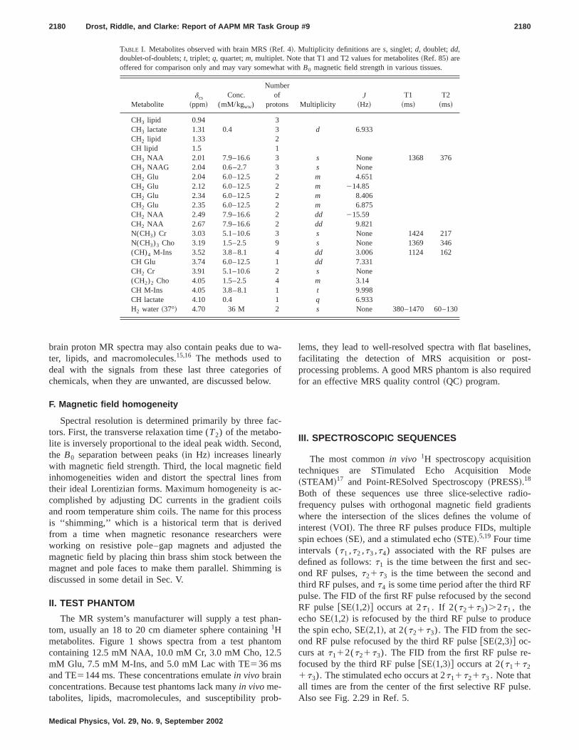
TABLE I. Metabolites observed with brain MRS~Ref. 4!. Multiplicity definitions ares, singlet;d, doublet;dd,doublet-of-doublets;t, triplet; q, quartet;m, multiplet. Note that T1 and T2 values for metabolites~Ref. 85! areoffered for comparison only and may vary somewhat withB0 magnetic field strength in various tissues.

Metabolitedcs

~ppm!Conc.

(mM/kgww)

Numberof

protons MultiplicityJ

~Hz!T1

~ms!T2

~ms!

CH3 lipid 0.94 3CH3 lactate 1.31 0.4 3 d 6.933CH2 lipid 1.33 2CH lipid 1.5 1CH3 NAA 2.01 7.9–16.6 3 s None 1368 376CH3 NAAG 2.04 0.6–2.7 3 s NoneCH2 Glu 2.04 6.0–12.5 2 m 4.651CH2 Glu 2.12 6.0–12.5 2 m 214.85CH2 Glu 2.34 6.0–12.5 2 m 8.406CH2 Glu 2.35 6.0–12.5 2 m 6.875CH2 NAA 2.49 7.9–16.6 2 dd 215.59CH2 NAA 2.67 7.9–16.6 2 dd 9.821N(CH3) Cr 3.03 5.1–10.6 3 s None 1424 217N(CH3)3 Cho 3.19 1.5–2.5 9 s None 1369 346(CH)4 M-Ins 3.52 3.8–8.1 4 dd 3.006 1124 162CH Glu 3.74 6.0–12.5 1 dd 7.331CH2 Cr 3.91 5.1–10.6 2 s None(CH2)2 Cho 4.05 1.5–2.5 4 m 3.14CH M-Ins 4.05 3.8–8.1 1 t 9.998CH lactate 4.10 0.4 1 q 6.933H2 water ~37°! 4.70 36 M 2 s None 380–1470 60–130

w

w.

c

nd

ldomcile

deththg

n

to5

b

es,t-ired

de

dio-ntsof

le

rec-d

Fond

ce

-

se.

brain proton MR spectra may also contain peaks due toter, lipids, and macromolecules.15,16 The methods used todeal with the signals from these last three categorieschemicals, when they are unwanted, are discussed belo

F. Magnetic field homogeneity

Spectral resolution is determined primarily by three fators. First, the transverse relaxation time (T2) of the metabo-lite is inversely proportional to the ideal peak width. Secothe B0 separation between peaks~in Hz! increases linearlywith magnetic field strength. Third, the local magnetic fieinhomogeneities widen and distort the spectral lines frtheir ideal Lorentizian forms. Maximum homogeneity is acomplished by adjusting DC currents in the gradient coand room temperature shim coils. The name for this procis ‘‘shimming,’’ which is a historical term that is derivefrom a time when magnetic resonance researchers wworking on resistive pole–gap magnets and adjustedmagnetic field by placing thin brass shim stock betweenmagnet and pole faces to make them parallel. Shimmindiscussed in some detail in Sec. V.

II. TEST PHANTOM

The MR system’s manufacturer will supply a test phatom, usually an 18 to 20 cm diameter sphere containing1Hmetabolites. Figure 1 shows spectra from a test phancontaining 12.5 mM NAA, 10.0 mM Cr, 3.0 mM Cho, 12.mM Glu, 7.5 mM M-Ins, and 5.0 mM Lac with TE536 msand TE5144 ms. These concentrations emulatein vivo brainconcentrations. Because test phantoms lack manyin vivo me-tabolites, lipids, macromolecules, and susceptibility pro

l. 29, No. 9, September 2002

a-

of

-

,

-sss

reeeis

-

m

-

lems, they lead to well-resolved spectra with flat baselinfacilitating the detection of MRS acquisition or posprocessing problems. A good MRS phantom is also requfor an effective MRS quality control~QC! program.

III. SPECTROSCOPIC SEQUENCES

The most commonin vivo 1H spectroscopy acquisitiontechniques are STimulated Echo Acquisition Mo~STEAM!17 and Point-RESolved Spectroscopy~PRESS!.18

Both of these sequences use three slice-selective rafrequency pulses with orthogonal magnetic field gradiewhere the intersection of the slices defines the volumeinterest~VOI!. The three RF pulses produce FIDs, multipspin echoes~SE!, and a stimulated echo~STE!.5,19 Four timeintervals (t1 ,t2 ,t3 ,t4) associated with the RF pulses adefined as follows:t1 is the time between the first and seond RF pulses,t21t3 is the time between the second anthird RF pulses, andt4 is some time period after the third Rpulse. The FID of the first RF pulse refocused by the secRF pulse@SE~1,2!# occurs at 2t1 . If 2(t21t3).2t1 , theecho SE~1,2! is refocused by the third RF pulse to produthe spin echo, SE~2,1!, at 2(t21t3). The FID from the sec-ond RF pulse refocused by the third RF pulse@SE~2,3!# oc-curs att112(t21t3). The FID from the first RF pulse refocused by the third RF pulse@SE~1,3!# occurs at 2(t11t2

1t3). The stimulated echo occurs at 2t11t21t3 . Note thatall times are from the center of the first selective RF pulAlso see Fig. 2.29 in Ref. 5.

nethec-hoil-di-ther

e.


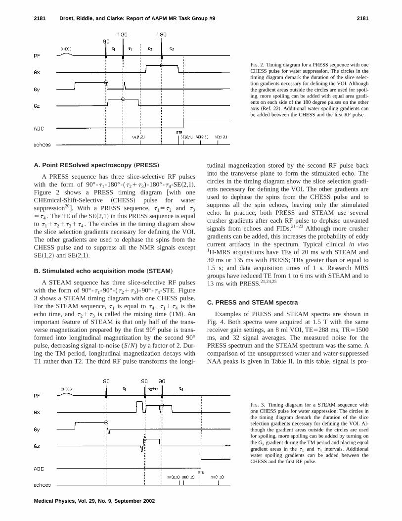
FIG. 2. Timing diagram for a PRESS sequence with oCHESS pulse for water suppression. The circles intiming diagram demark the duration of the slice seletion gradients necessary for defining the VOI. Althougthe gradient areas outside the circles are used for sping, more spoiling can be added with equal area graents on each side of the 180 degree pulses on the oaxis ~Ref. 22!. Additional water spoiling gradients canbe added between the CHESS and the first RF puls

ls

a

O

e

lse

e

s-n0

ithg

ackhe

di-ared toted

eralnted

ddy

dl toRSto

inme

thee. Assed-

A. Point RESolved spectroscopy „PRESS…

A PRESS sequence has three slice-selective RF puwith the form of 90°-t1-180°-(t21t3)-180°-t4-SE~2,1!.Figure 2 shows a PRESS timing diagram@with oneCHEmical-Shift-Selective ~CHESS! pulse for watersuppression20#. With a PRESS sequence,t15t2 and t3

5t4 . The TE of the SE~2,1! in this PRESS sequence is equto t11t21t31t4 . The circles in the timing diagram showthe slice selection gradients necessary for defining the VThe other gradients are used to dephase the spins fromCHESS pulse and to suppress all the NMR signals excSE~1,2! and SE~2,1!.

B. Stimulated echo acquisition mode „STEAM…

A STEAM sequence has three slice-selective RF puwith the form of 90°-t1-90°-(t21t3)-90°-t4-STE. Figure3 shows a STEAM timing diagram with one CHESS pulsFor the STEAM sequence,t1 is equal tot4 , t11t4 is theecho time, andt21t3 is called the mixing time~TM!. Animportant feature of STEAM is that only half of the tranverse magnetization prepared by the first 90° pulse is traformed into longitudinal magnetization by the second 9pulse, decreasing signal-to-noise (S/N) by a factor of 2. Dur-ing the TM period, longitudinal magnetization decays wT1 rather than T2. The third RF pulse transforms the lon


es

l

I.thept

s

.

s-°

i-

tudinal magnetization stored by the second RF pulse binto the transverse plane to form the stimulated echo. Tcircles in the timing diagram show the slice selection graents necessary for defining the VOI. The other gradientsused to dephase the spins from the CHESS pulse ansuppress all the spin echoes, leaving only the stimulaecho. In practice, both PRESS and STEAM use sevcrusher gradients after each RF pulse to dephase unwasignals from echoes and FIDs.21–23 Although more crushergradients can be added, this increases the probability of ecurrent artifacts in the spectrum. Typical clinicalin vivo1H-MRS acquisitions have TEs of 20 ms with STEAM an30 ms or 135 ms with PRESS; TRs greater than or equa1.5 s; and data acquisition times of 1 s. Research Mgroups have reduced TE from 1 to 6 ms with STEAM and13 ms with PRESS.21,24,25

C. PRESS and STEAM spectra

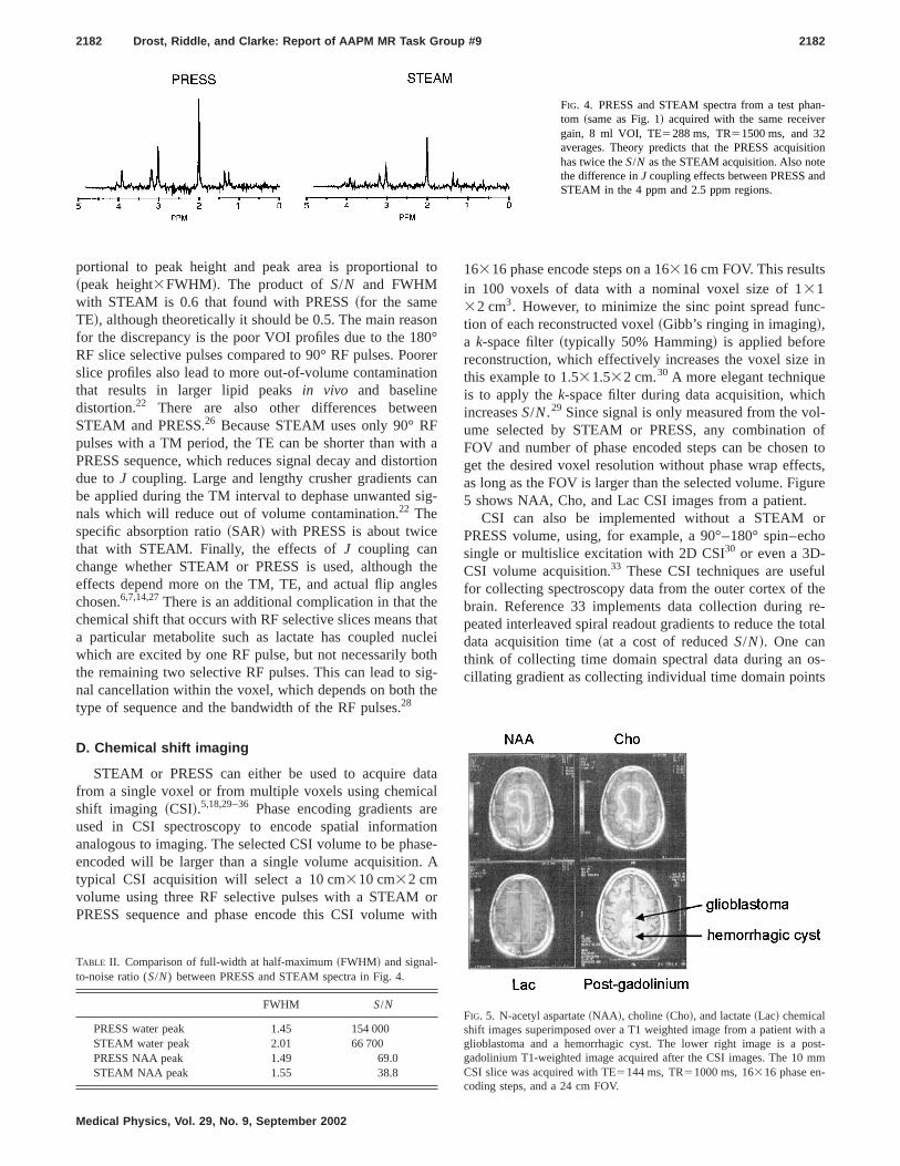
Examples of PRESS and STEAM spectra are shownFig. 4. Both spectra were acquired at 1.5 T with the sareceiver gain settings, an 8 ml VOI, TE5288 ms, TR51500ms, and 32 signal averages. The measured noise forPRESS spectrum and the STEAM spectrum was the samcomparison of the unsuppressed water and water-suppreNAA peaks is given in Table II. In this table, signal is pro

hinel-

sedn

al

the

FIG. 3. Timing diagram for a STEAM sequence witone CHESS pulse for water suppression. The circlesthe timing diagram demark the duration of the slicselection gradients necessary for defining the VOI. Athough the gradient areas outside the circles are ufor spoiling, more spoiling can be added by turning otheGy gradient during the TM period and placing equgradient areas in thet1 and t4 intervals. Additionalwater spoiling gradients can be added betweenCHESS and the first RF pulse.

n-r

tion

d


FIG. 4. PRESS and STEAM spectra from a test phatom ~same as Fig. 1! acquired with the same receivegain, 8 ml VOI, TE5288 ms, TR51500 ms, and 32averages. Theory predicts that the PRESS acquisihas twice theS/N as the STEAM acquisition. Also notethe difference inJ coupling effects between PRESS anSTEAM in the 4 ppm and 2.5 ppm regions.

l t

o0oio

enFhrta

sig

thleethco

sith

aalretioas. A

ow

c-

in

hl-ofn to

cts,ure

orcho

ulthere-total

s-ts

ith aost-mm

portional to peak height and peak area is proportiona~peak height3FWHM!. The product ofS/N and FWHMwith STEAM is 0.6 that found with PRESS~for the sameTE!, although theoretically it should be 0.5. The main reasfor the discrepancy is the poor VOI profiles due to the 18RF slice selective pulses compared to 90° RF pulses. Poslice profiles also lead to more out-of-volume contaminatthat results in larger lipid peaksin vivo and baselinedistortion.22 There are also other differences betweSTEAM and PRESS.26 Because STEAM uses only 90° Rpulses with a TM period, the TE can be shorter than witPRESS sequence, which reduces signal decay and distodue toJ coupling. Large and lengthy crusher gradients cbe applied during the TM interval to dephase unwantednals which will reduce out of volume contamination.22 Thespecific absorption ratio~SAR! with PRESS is about twicethat with STEAM. Finally, the effects ofJ coupling canchange whether STEAM or PRESS is used, althougheffects depend more on the TM, TE, and actual flip angchosen.6,7,14,27There is an additional complication in that thchemical shift that occurs with RF selective slices meansa particular metabolite such as lactate has coupled nuwhich are excited by one RF pulse, but not necessarily bthe remaining two selective RF pulses. This can lead tonal cancellation within the voxel, which depends on bothtype of sequence and the bandwidth of the RF pulses.28

D. Chemical shift imaging

STEAM or PRESS can either be used to acquire dfrom a single voxel or from multiple voxels using chemicshift imaging ~CSI!.5,18,29–36 Phase encoding gradients aused in CSI spectroscopy to encode spatial informaanalogous to imaging. The selected CSI volume to be phencoded will be larger than a single volume acquisitiontypical CSI acquisition will select a 10 cm310 cm32 cmvolume using three RF selective pulses with a STEAMPRESS sequence and phase encode this CSI volume

TABLE II. Comparison of full-width at half-maximum~FWHM! and signal-to-noise ratio (S/N) between PRESS and STEAM spectra in Fig. 4.

FWHM S/N

PRESS water peak 1.45 154 000STEAM water peak 2.01 66 700PRESS NAA peak 1.49 69.0STEAM NAA peak 1.55 38.8


o

n°rern

aionn-

es

atleithg-e

ta

ne-

rith

16316 phase encode steps on a 16316 cm FOV. This resultsin 100 voxels of data with a nominal voxel size of 13132 cm3. However, to minimize the sinc point spread funtion of each reconstructed voxel~Gibb’s ringing in imaging!,a k-space filter~typically 50% Hamming! is applied beforereconstruction, which effectively increases the voxel sizethis example to 1.531.532 cm.30 A more elegant techniqueis to apply thek-space filter during data acquisition, whicincreasesS/N.29 Since signal is only measured from the voume selected by STEAM or PRESS, any combinationFOV and number of phase encoded steps can be choseget the desired voxel resolution without phase wrap effeas long as the FOV is larger than the selected volume. Fig5 shows NAA, Cho, and Lac CSI images from a patient.

CSI can also be implemented without a STEAMPRESS volume, using, for example, a 90°–180° spin–esingle or multislice excitation with 2D CSI30 or even a 3D-CSI volume acquisition.33 These CSI techniques are useffor collecting spectroscopy data from the outer cortex ofbrain. Reference 33 implements data collection duringpeated interleaved spiral readout gradients to reduce thedata acquisition time~at a cost of reducedS/N!. One canthink of collecting time domain spectral data during an ocillating gradient as collecting individual time domain poin

FIG. 5. N-acetyl aspartate~NAA !, choline~Cho!, and lactate~Lac! chemicalshift images superimposed over a T1 weighted image from a patient wglioblastoma and a hemorrhagic cyst. The lower right image is a pgadolinium T1-weighted image acquired after the CSI images. The 10CSI slice was acquired with TE5144 ms, TR51000 ms, 16316 phase en-coding steps, and a 24 cm FOV.

mc

en

ge

ee

ca

A.

doth

nutehee

timtrhen

teat

by

nsina

ly-n

-

etSb

xelnsint

ionbedis-ent

isTEthe

iteTEA,

e-hatsiveperrp-

ak.

as,

qual-areak isalin

silybe

ion

e,ion

himni--om,

ar-


for a repeating series ofk-space points.34 Only a few timedomain points are collected at eachk-space point during asingle TR, but repeated data acquisitions with different tidelays will produce a complete time domain signal for eak-space point. These advanced techniques are not curravailable in a commercial product.

E. Single voxel vs chemical shift imaging

Proton MRS with CSI acquisition has several advantaover single voxel acquisitions~SVA!.

~1! CSI provides betterS/N as compared to two or morsequential SVA since the signal from each voxel is avaged for the total data collection time with CSI.

~2! The CSI grid can be shifted after data acquisition~simi-lar to image scrolling!, allowing precise positioning of avoxel after data acquisition.

~3! Many more voxels of data are collected in a practiacquisition time.

There are also disadvantages of CSI compared to SV

~1! Since with CSI only the whole CSI volume is shimmerather than each individual voxel as in SVA, the shim feach CSI voxel is not as good as on a SVA voxel insame location.

~2! The poorer shim causes more problems with lipid cotamination although additional techniques, such as ovolume suppression~OVS!, can be used to reducthis.23,29,32 Water suppression will also vary across tCSI volume because of both changes in B1 and magnfield inhomogeneities.

~3! Because three ‘‘slice’’ selective RF pulses are usedselect the CSI PRESS or STEAM volume, there areperfect slice profiles which cause problems for specfrom voxels near the outside of the CSI volume. Tresulting alterations in tip angle and phase for differevoxel locations will alterJ coupling effects as a functionof location that in turn will make consistent metaboliquantification more difficult. Nonoptimal tip anglesthe outer edges of the CSI volume also reduceS/N in theouter voxels.

~4! The minimum CSI data collection time is determinedthe required number of phase encode steps and cancome long, especially if an unsuppressed water refereset is required. Time cannot be reduced by decreathe size ofk space since this increases lipid contamintion from the CSI point spread function.30 The acquisi-tion time can be reduced by 25% with a circularboundedk-space acquisition,35 a reduced FOV and number of phase encoded steps across the narrow directiothe head37 ~similar to a rectangular field of view in imaging!, or with the echo planar imaging~EPI! spectros-copy approach.33,34

~5! The metabolite concentrations measured from a sptrum associated with one voxel actually correspondthe integrated metabolite concentrations over the Cpoint spread function. This means the measured meta


ehtly

s

r-

l

re

-er

tic

o-a

t

be-ceg

-

of

c-oIo-

lite concentrations will depend on such factors as volocation and how quickly metabolite concentratiochange spatially throughout the brain. Since the pospread function usually has negative lobes~sinc func-tion! and spectra quantification is done in the absorptmode, metabolite peaks from adjacent voxels willadded in negative phase. This will cause peak shapetortions because adjacent voxels usually have differcenter frequencies than the voxel of interest.

In summary, consistent, high quality, short TE spectrainvivo are best acquired with the SVA technique,38 but timerestraints limit acquiring data from only a few VOIs. CSIbest when more VOIs are required. A long echo time (.130 ms) can be used to simplify the spectra and reducelipid and macromolecule signal, which will make metabolquantification reasonably consistent. However, the longtime reduces the number of quantified metabolites to NACho, Cr, and lactate.

IV. SIGNAL-TO-NOISE RATIO

Since the MRS time domain signal is complex, two frquency domain signals result from the Fourier transform tare typically labeled ‘‘real’’ and ‘‘imaginary.’’ These signalare linear combinations of the absorptive and disperscomponents of the Lorentzian line shape. In principle prophase adjustments can make the ‘‘real’’ signal purely absotive and the ‘‘imaginary’’ signal purely dispersive.

The signal from a metabolite is the area under its peThe full-width at half-maximum value~FWHM! of theLorentzian absorption spectral peak in Hz is definedFWHM51/(pT2* ), where 1/T2* 51/T21gDB0 . For anabsorptive Lorentzian peak the area under the peak is eto p/2* (FWHM)* ~peak height!. For the Lorentzian dispersion component, the peak width is much broader and theunder the peak integrates to zero, so the dispersion peanot typically used in clinical MRS analysis. A mathematicdescription of the Lorentzian function can be found belowSec. XV.

In a well-shimmed spectrum, the peak’s height is an eameasured indicator of the signal. Noise in a spectrum canevaluated by measuring the standard deviation in a regthat contains no signal, such as between21.0 and 22.0ppm. Therefore, one definition ofS/N is the ratio of peakheight divided by the rms noise.27 Under this definition, onemanufacturer suggests that the minimum acceptablein vivoS/N is five. A second definition ofS/N is peak area dividedby the rms noise.39 Both definitions are used in the literaturbut careful reading may be required to learn which definita particular paper uses.

The area of a Lorentzian peak is independent of the squality measured by FWHM. Therefore, the second defition is a more absolute measure ofS/N and a better parameter for testing hardware performance on a MRS phantespecially for quality control~QC! and for comparing differ-ent hardware. However,in vivo, metabolite peaks typicallyoverlap and the precision in determining metabolite peak

ss


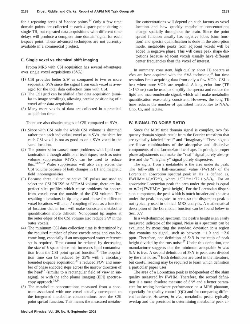
FIG. 6. Effect of changing VOI size on SIGNAL andNOISE. The head coil has more SIGNAL and leNOISE than the body coil.

y.at

alc

Mea

emeaar

ORo

I,

tisil

lea

chn

ilialtos

s

hin

ngcqat

yngightheales

ncev-

ndto-theor

derd aare

hehefol-

alard

aher

E

m.ter attleand

eas depends as much on the FWHM as on the peak areaS/N.Therefore, the first definition ofS/N is more pertinent forcomparingin vivo data and optimizing MRS methodologNote, however, that metabolite concentrations are calculfrom peak areas. In addition, when comparingS/N betweentwo spectra, the comparison will be valid only if identicdata acquisition and post-processing were used. Theseditions are rarely met when spectra are collected onsystems from two different vendors. As an example, parea which is proportional to the amplitude of the first timdomain point is usually not affected by post-processing tidomain filters, but these filters reduce noise and pheights. Therefore post-processing filters change peakS/N differently than peak heightS/N.

The magnitude of the noise is independent of the Vsize, but depends on the tissue volume detected by thecoil, and increases with the square root of the numbersignals that were added coherently~n!. The magnitude of thesignal is directly proportional to the volume of the VOproton density, and the number of averages~n!. Figure 6shows the noise and signal in the head and body coils asVOI size is changed. With respect to the head coil, the nois 14% higher and the signal 76% lower with the body coWith averaging,S/N is proportional ton/An, or An.

Averaging is a specific example illustrating the principthatS/N is proportional to the square root of the total signdata acquisition time.40 Therefore,S/N ~peak height! willalso depend on the duration of the STEAM or PRESS ewhich decays with T2* , assuming that the data acquisitiotime is >5T2* in duration. The specific value of T2* willdepend on the shim, metabolite T2, and tissue susceptibA good single voxel shim in the brain’s parietal–occipitlobe will give a linewidth approaching 4 Hz correspondinga T2* 580 ms.In vitro on a spherical phantom, voxel shimbelow 1 Hz are typical corresponding to a T2* .318 ms.Therefore,in vivo, an echo data acquisition time of 400 m(53T2* ) is sufficient, butin vitro, data acquisition times.1500 ms are required to maximizeS/N. When comparingtwo different MR systems onS/N, one must ensure that botsystems are using the same data acquisition time. Also, sin a typical in vivo 1H-MRS acquisition TR is>1.5 s allow-ing a data acquisition time>1 s,S/N will increase from thelonger signal duration obtained with better shimming.

Depending on the system software, two of the followithree parameters must be set prior to a spectroscopy asition: the data acquisition time, the number of complex d


ed

on-Rk

ekea

IFf

hee.

l

o

ty.

ce

ui-a

points, or the sampling frequency~bandwidth! of the analog-to-digital converter~A/D!. Setting two of these automaticallcalculates the other. Besides having a sufficiently loenough data acquisition time one must also have a henough sampling frequency to cover the bandwidth ofdesired spectrum. Note that this required bandwidth sclinearly with B0 .

V. SHIMMING

The preceding sections have emphasized the importaof magnetic field homogeneity in MR spectroscopy. Improing magnetic field homogeneity increasesS/N and narrowspeak widths. Thus shimming improves both sensitivity aspectral resolution. Modern clinical MRI systems use aumated shimming routines to improve the homogeneity ofmagnetic field by monitoring either the time-domainfrequency-domain MRS signal.41–46 Note that most clinicalMR systems only have first-order shims~gradient coil DCoffsets! but a few systems have an additional second-orroom-temperature shim set. Examples of a good shim anbad shim in the water and water-suppressed signalsshown in Figs. 7 and 8. Note that the water signal~unsup-pressed! is always used for shimming.

The autoshimming algorithm of the MR system and tmagnet B0 homogeneity can be evaluated by using tspherical MRS phantom. The evaluation should meet thelowing criteria.

Global shim: After applying the manufacturer’s clinicauto shim software, usually over a 25 cm FOV, a simple hRF pulse~typically a 200–500ms rectangular pulse! plussignal readout without gradients~data acquisition time.300 ms! should show a water peak with a FWHM<5 Hzand a full-width at tenth-maximum (FWTM)<53FWHM.This last condition on the FWTM is calculated assumingLorentzian line shape and is sensitive to second and higorder magnetic field inhomogeneities. Typical headin vivoshims range from 12–20 Hz, FWHM.

Localized shim: Select a single voxel short echo (T<30 ms) STEAM or PRESS sequence and place a 23232 cm3 voxel at approximately the center of the phantoAcquire an unsuppressed water spectrum before and afmanual or localized auto shim. Ideally, there should be lior no change in peak width between the two acquisitionsthe FWHM should be,1 Hz, or a T2* .318 ms. The dataacquisition time must be greater than 53T2* and the phan-

lls

l

lls

l

ee


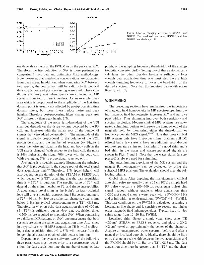
FIG. 7. Example of a good shim. Pane~A! contains the two received channe~light lines! and the magnitude of thewater signal in the time domain. Pane~B! contains the absorption spectrumfrom the water with a FWHM of 1.9Hz. Panel ~C! shows the absorptionspectrum with water suppression.

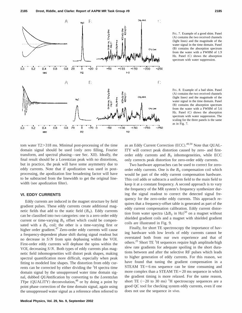
FIG. 8. Example of a bad shim. Pane~A! contains the two received channe~light lines! and the magnitude of thewater signal in the time domain. Pane~B! contains the absorption spectrumfrom the water with a FWHM of 5.6Hz. Panel ~C! shows the absorptionspectrum with water suppression. Thscaling for the three panels is the samas in Fig. 7.

e

nstsve

ea

d-ret b.thg-inaur

si

ined

t-

.ero-

re.toaryur-

fre-re-

f thetor-

ient

v-beofhra-adswea

nd

on,ane

tom water T2.318 ms. Minimal post-processing of the timdomain signal should be used~only zero filling, Fouriertransform, and spectral phasing—see Sec. XII!. Ideally, thefinal result should be a Lorentzian peak with no distortiobut in practice, the peak will have some asymmetry dueeddy currents. Note that if apodization was used in poprocessing, the apodization line broadening factor will hato be subtracted from the linewidth to get the original linwidth ~see apodization filter!.

VI. EDDY CURRENTS

Eddy currents are induced in the magnet structure by figradient pulses. These eddy currents create additional mnetic fields that add to the static field (B0). Eddy currentscan be classified into two categories: one is a zero order ecurrent or time-varyingB0 offset which could be compensated with aB0 coil; the other is a time-varying first ohigher order gradient.47 Zero-order eddy currents will causa frequency-dependent phase shift during signal readouno decrease inS/N from spin dephasing within the VOIFirst-order eddy currents will dephase the spins withinVOI, decreasingS/N. Both types of eddy currents plus manetic field inhomogeneities will distort peak shapes, makspectral quantification more difficult, especially when pefitting to modeled line shapes. The distortion from eddy crents can be corrected by either dividing the1H spectra timedomain signal by the unsuppressed water time domainnal, dubbedQUAntification by converting to theLorentzIanTYpe ~QUALITY ! deconvolution,48 or by doing a point bypoint phase correction of the time domain signal, again usthe unsuppressed water signal as a reference often referr


,ot-e-

ldg-

dy

ut

e

gk-

g-

gto

as an Eddy Current Correction~ECC!.49,50 Note that QUAL-ITY will correct peak distortion caused by zero- and firsorder eddy currents andB0 inhomogeneities, while ECConly corrects peak distortion for zero-order eddy currents

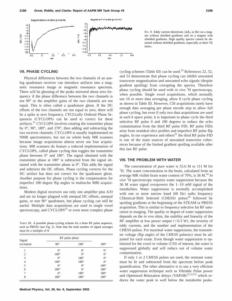
Two hardware approaches can be used to correct for zorder eddy currents. One is theB0 compensation coil whichwould be part of the eddy current compensation hardwaThis coil adds or subtracts a uniform field to the main fieldkeep it at a constant frequency. A second approach is to vthe frequency of the MR system’s frequency synthesizer ding the signal readout to correct the detected signalquency for the zero-order eddy currents. This approachquires that a frequency-offset table is generated as part oeddy current compensation calibration. Eddy current distion from water spectra~DB0 in Hz!50 on a magnet withoutshielded gradient coils and a magnet with shielded gradcoils are illustrated in Fig. 9.

Finally, for short TE spectroscopy the importance of haing hardware with low levels of eddy currents cannotoverstated both from our own experience and thatothers.25 Short TE1H sequences require high amplitude/higslew rate gradients for adequate spoiling in the short dutions between and after the selective RF pulses which leto higher generation of eddy currents. For this reason,have found that tuning the gradient compensation inSTEAM TE56 ms sequence can be time consuming amore complex than a STEAM TE520 ms sequence in whichthe gradient timing is more relaxed. For the same reasshort TE ~;20 to 30 ms! 1H spectroscopy sequences aregood QC tool for checking system eddy currents, even if odoes not use the sequencein vivo.

ithb-

TE


FIG. 9. Eddy current distortions~DB0 in Hz! on a mag-net without shielded gradients and on a magnet wshielded gradients. High quality spectra cannot be otained without shielded gradients, especially at shorttimes.

nagrurelsnoDCw

esethoeruinttethontsfo

si

/Du

l bxee

,ted

e

llylingvefull

sedirdchos

flip

her-fter

oran

thehehed

SStu-ion

themit-

op-

ter

tereakent

ks.

nces

VII. PHASE CYCLING

Physical differences between the two channels of an alog quadrature receiver can introduce artifacts into a mnetic resonance image or magnetic resonance spectThere will be ghosting of the peaks mirrored about zero fquency if the phase difference between the two channenot 90° or the amplifier gains of the two channels areequal. This is often called a quadrature ghost. If theoffsets of the two channels are not equal to zero, therebe a spike at zero frequency.CYCLically OrderedPhaseSe-quences~CYCLOPS! can be used to correct for thesartifacts.51 CYCLOPS involves rotating the transmitter phaby 0°, 90°, 180°, and 270°, then adding and subtractingtwo receiver channels. CYCLOPS is usually implementedNMR spectrometers, but not on whole body MR scannbecause image acquisitions almost never use four acqtions. MR scanners do feature a reduced implementatioCYCLOPS, called phase cycling that toggles the transmiphase between 0° and 180°. The signal obtained withtransmitter phase at 180° is subtracted from the signaltained with the transmitter phase at 0°. This adds the sigand subtracts the DC offsets. Phase cycling corrects forDC artifact but does not correct for the quadrature ghoAnother purpose for phase cycling is the compensationimperfect 180 degree flip angles in multiecho MRI acquitions.

Modern digital receivers use only one amplifier plus Aand are no longer plagued with unequal DC offsets, uneqgains, or non 90° quadrature, but phase cycling can stiluseful. Multiple data acquisitions are used in single vospectroscopy, and CYCLOPS52 or even more complex phas

TABLE III. A possible phase-cycling scheme for a three RF pulse sequesuch as PRESS~see Fig. 2!. Note that the total number of signal averagmust be a multiple of 8.

Signalexcitation

RF pulse phase

90° 180° 180°

1 0° 0° 0°2 180° 0° 0°3 0° 180° 0°4 180° 180° 0°5 0° 0° 180°6 180° 0° 180°7 0° 180° 180°8 180° 180° 180°


a--m.-ist

ill

enssi-ofre

b-alhet.r

-

alel

cycling schemes~Table III! can be used.53 References 22, 52and 53 demonstrate that phase cycling can inhibit unwantransverse magnetization and unwanted echo signals~despitegradient spoiling! from corrupting the spectra. Thereforphase cycling should be used within vivo 1H spectroscopy,when possible. Single voxel acquisitions, which normause 16 or more data averaging, allow 8 cycle phase cycas shown in Table III. However, CSI acquisitions rarely haenough data averaging per phase encode step to allowphase cycling, but even if only two data acquisitions are uat eachk space point, it is important to phase cycle the thselective RF pulse 0 and 180 degrees to reduce the econtamination from the third RF pulse FID. RF pulse FIDarise from nonideal slice profiles and imperfect RF pulseangles. In our experience and others22 the third RF pulse FIDis one of the main sources of unwanted transverse coences because of the limited gradient spoiling available athis last RF pulse.

VIII. THE PROBLEM WITH WATER

The concentration of pure water is 55.6 M or 111 M f1H. The water concentration in the brain, calculated fromaverage MR visible brain water content of 70%, is 36 M.54 Invivo 1H spectroscopy requires water suppression because36 M water signal overpowers the 1–10 mM signal of tmetabolites. Water suppression is normally accompliswith one or more narrow band~60 Hz! radio frequencyCHemical-Shift Selected~CHESS! pulses20 followed byspoiling gradients at the beginning of the STEAM or PREacquisition. This is similar to frequency selective fat RF saration in imaging. The quality or degree of water suppressdepends on thein vivo shim, the stability and linearity of theRF amplifier at low power output~,0.3 W!, the severity ofeddy currents, and the number and implementation ofCHESS pulses. For maximal water suppression, the transter voltage~flip angle! of the CHESS pulses~s! must be ad-justed for each exam. Even though water suppression istimized for the voxel or volume~CSI! of interest, the water issuppressed globally and will reduce out of volume wacontamination.

If only 1 or 2 CHESS pulses are used, the remnant wamust be fit and subtracted from the spectrum before pquantification. The other alternative is to use a very efficiwater suppression technique such asVAriable Pulse powerandOptimizedRelaxation delays~VAPOR!21,23,55which re-duces the water peak to well below the metabolite pea

e,

m

Re9.ee

il-


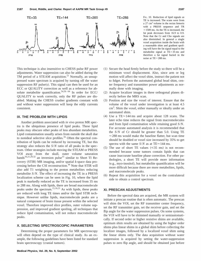
FIG. 10. Reduction of lipid signals asTE is increased. The scans were froa 27 cm3 volume in the rectus femoriswith a PRESS sequence and T51500 ms. As the TE is increased, thfat peak decreases from 16.9 to 0.Note that the Cr and Cho signals aralso diminished. In general a singlvoxel acquisition inside the brain witha reasonable shim and gradient spoing will have the fat signal equal to themetabolite signal at TE535 ms andtherefore a fat signal buried in thenoise at TE5288 ms.

wg

atnb-

-i

n

piliu-hi-Sn

-

inS

ipm

ul

h

ctep

thle

opx-ar

e ag

oten-or-

di-

the.5n

heles

thatEmeget

canr pa-n

ids,

ral

willcancy,t thems,ti-le,

derthengtersionfore

This technique is also insensitive to CHESS pulse RF poadjustments. Water suppression can also be added durinTM period of a STEAM acquisition.21 Normally, an unsup-pressed water spectrum is acquired by turning off the wsuppression RF pulse~s!. This signal can then be used for aECC or QUALITY correction as well as a reference for asolute metabolite quantification.54,56–64 In order for ECC/QUALITY to work correctly, only the RF pulses are disabled. Making the CHESS crusher gradients constant wand without water suppression will keep the eddy curreconsistent.

IX. THE PROBLEM WITH LIPIDS

Another problem associated within vivo proton MR spec-tra is the ubiquitous presence of lipid peaks. These lipeaks may obscure other peaks of less abundant metaboLipid contamination usually arises from outside the skull dto nonideal selective slice profiles.16 Often the spectral contribution of lipids can be reduced by increasing TE, but tstrategy also reduces theS/N ratio of all peaks in the spectrum. Other strategies include moving the STEAM or PREVOI away from the skull, outer volume saturatiobands16,21,29,32an inversion pulse15 similar to Short TI Re-covery~STIR! MR imaging, and/or spatialk-space data processing before the CSI reconstruction.36 Note that STIR willalso add T1 weighting to the proton metabolites reducmetaboliteS/N. The effect of increasing the TE in a PRESlocalization scheme can be seen in Fig. 10, where the lpeak is markedly reduced as the TE is increased from 35to 288 ms. Along with lipids, there are broad macromolecpeaks under the spectrum.15,16,21As with lipids, these peaksare reduced with long TE times and/or the lipid STIR tecnique. However unlike lipids, macromolecule peaks arenatural component of brain tissue present within the selevoxel. Therefore improved slice profiles, outer volume supression, and improved gradient spoiling, all techniquesreduce lipid contamination, will not reduce macromolecupeaks.

X. SELECTING SPECTROSCOPIC PARAMETERS

Determining the proper parameters for MR spectroscwill often depend on the type of clinical study. As an eample, the following guidelines have been listed for standbrain spectroscopy~cranial tumors!.


erthe

er

thts

dtes.e

s

S

g

ids

e

-ad

-at

y

d

~1! Secure the head firmly before the study so there will bminimum voxel displacement. Also, since arm or lemotion will affect the voxel shim, instruct the patient nto fidget. Perform the automated global head shim, cter frequency and transmitter power adjustments as nmally done with imaging.

~2! Acquire localizer images in three orthogonal planesrectly before the MRS scan.

~3! Position and size the voxel of interest. Ensure thatvolume of the voxel under investigation is at least 4cm3. Shim the voxel, either manually or ideally under aautomated shim.

~4! Use a TE'144 ms and acquire about 128 scans. Tlater echo time reduces the signal from macromolecuand from lipid contamination while retaining goodS/N.For accurate automated analysis it is recommendedthe S/N of Cr should be greater than 5.0. Using T'288 ms would make the baseline flatter, but scan tishould be doubled or voxel size increased by 35% tospectra with the sameS/N as at TE'144 ms.

~5! The use of short TE values~<35 ms! is not recom-mended because some tumors contain lipids thatcause inaccurate baseline phase correction. For othethologies, a short TE will provide more informatio~e.g., myo-inositol!, but metabolite quantification will bemore difficult because there are more metabolites, lipand macromolecule peaks.

~6! Repeat this acquisition for a voxel on the contralateside to obtain a control spectrum.

XI. PRESCAN ADJUSTMENTS

Before the spectral data are acquired, the MR systeminitiate a prescan routine that is often automatic. The preswill shim the VOI, set the RF transmitter center frequenset the RF transmitter gain, set the receiver gain, and seflip angle for the water suppression pulses. On some systethe VOI will have to be shimmed manually or semiautomacally. If second order or higher resistive shims are availaboptimum shim results are obtained by using the higher orshims plus linear shims in a global shim before collectinglocalizer images, followed by a localized voxel shim usithe linear shims only. The data acquisition without wasuppression is acquired by setting the water-supprespulses to zero flip angle, and should be obtained just be

TEreht

-wsce-

alionat

hase-um.


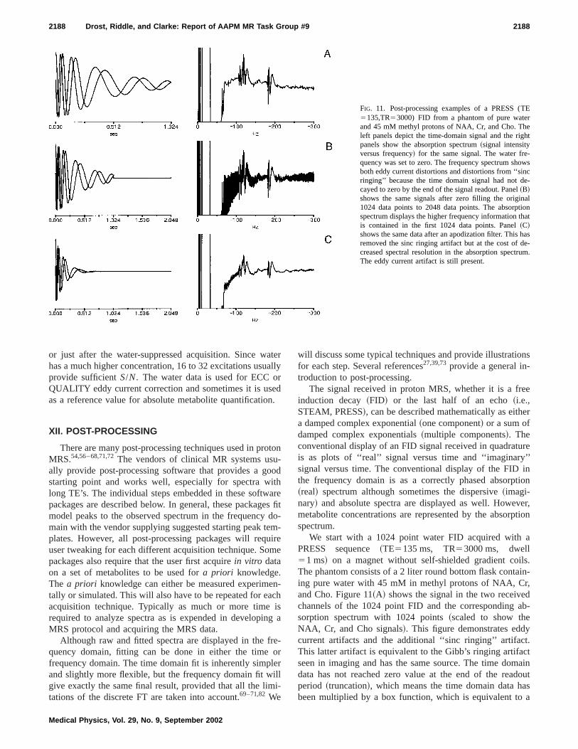
FIG. 11. Post-processing examples of a PRESS (5135,TR53000) FID from a phantom of pure wateand 45 mM methyl protons of NAA, Cr, and Cho. Thleft panels depict the time-domain signal and the rigpanels show the absorption spectrum~signal intensityversus frequency! for the same signal. The water frequency was set to zero. The frequency spectrum shoboth eddy current distortions and distortions from ‘‘sinringing’’ because the time domain signal had not dcayed to zero by the end of the signal readout. Panel~B!shows the same signals after zero filling the origin1024 data points to 2048 data points. The absorptspectrum displays the higher frequency information this contained in the first 1024 data points. Panel~C!shows the same data after an apodization filter. Thisremoved the sinc ringing artifact but at the cost of dcreased spectral resolution in the absorption spectrThe eddy current artifact is still present.

atar

edn

ot-

ooithaed

emuirm

encis

ng

reo

leilli

ns

ee

er

ure’’intion

ver,tion

a

ls.-,dab-

yt.ct

aindoutasa

or just after the water-suppressed acquisition. Since whas a much higher concentration, 16 to 32 excitations usuprovide sufficientS/N. The water data is used for ECC oQUALITY eddy current correction and sometimes it is usas a reference value for absolute metabolite quantificatio

XII. POST-PROCESSING

There are many post-processing techniques used in prMRS.54,56–68,71,72The vendors of clinical MR systems usually provide post-processing software that provides a gstarting point and works well, especially for spectra wlong TE’s. The individual steps embedded in these softwpackages are described below. In general, these packagmodel peaks to the observed spectrum in the frequencymain with the vendor supplying suggested starting peak tplates. However, all post-processing packages will requser tweaking for each different acquisition technique. Sopackages also require that the user first acquirein vitro dataon a set of metabolites to be used fora priori knowledge.The a priori knowledge can either be measured experimtally or simulated. This will also have to be repeated for eaacquisition technique. Typically as much or more timerequired to analyze spectra as is expended in developiMRS protocol and acquiring the MRS data.

Although raw and fitted spectra are displayed in the fquency domain, fitting can be done in either the timefrequency domain. The time domain fit is inherently simpand slightly more flexible, but the frequency domain fit wgive exactly the same final result, provided that all the limtations of the discrete FT are taken into account.69–71,82We


erlly

.

on

d

res fito--

ee

-h

a

-rr

-

will discuss some typical techniques and provide illustratiofor each step. Several references27,39,73provide a general in-troduction to post-processing.

The signal received in proton MRS, whether it is a frinduction decay~FID! or the last half of an echo~i.e.,STEAM, PRESS!, can be described mathematically as eitha damped complex exponential~one component! or a sum ofdamped complex exponentials~multiple components!. Theconventional display of an FID signal received in quadratis as plots of ‘‘real’’ signal versus time and ‘‘imaginarysignal versus time. The conventional display of the FIDthe frequency domain is as a correctly phased absorp~real! spectrum although sometimes the dispersive~imagi-nary! and absolute spectra are displayed as well. Howemetabolite concentrations are represented by the absorpspectrum.

We start with a 1024 point water FID acquired withPRESS sequence~TE5135 ms, TR53000 ms, dwell51 ms! on a magnet without self-shielded gradient coiThe phantom consists of a 2 liter round bottom flask containing pure water with 45 mM in methyl protons of NAA, Crand Cho. Figure 11~A! shows the signal in the two receivechannels of the 1024 point FID and the correspondingsorption spectrum with 1024 points~scaled to show theNAA, Cr, and Cho signals!. This figure demonstrates eddcurrent artifacts and the additional ‘‘sinc ringing’’ artifacThis latter artifact is equivalent to the Gibb’s ringing artifaseen in imaging and has the same source. The time domdata has not reached zero value at the end of the reaperiod ~truncation!, which means the time domain data hbeen multiplied by a box function, which is equivalent to

ls

c-heis

or

,-

t

inuma

nadr

in

inino-ath

entthl-.

d

cye

ele

he

-

-hasehashashat

ros-st-to

nalcyell

heo-

rnalswa-ab-

r,heraksandh

ofou-andg aleyrmted

last

o-tC

0.


sinc convolution in the frequency domain. This effect is areferred to as leakage.39

A. Zero filling

Zero filling in the time domain is equivalent to a sinconvolution~interpolation! in the frequency domain. This interpolation improves the visual display of the data in tfrequency domain, although no additional informationadded. This is identical to image interpolation in MRI. Fexample, anN point FID hasN real andN imaginary, or 2Npoints sampled atDt intervals. After Fourier transformationthere areN real andN imaginary points with frequency spacing equal to 1/(NDt). The spectral width~SW! of the spec-trum is 1/Dt with the abscissa going from SW/2 to2SW/2.Zeros can be added to the end of the FID to decreasefrequency spacing over the same bandwidth. Figure 11~B!illustrates zero filling the 1024 point FID to 2048 pointsthe time domain and the resultant absorption spectrwhich increases the display of the higher frequencies thatcontained in the original 1024 data set.

B. Apodization filter

The signal in a free induction decay contains the sigfrom the metabolites being studied and the noise in thetector channels. A line broadening filter decreases theceived signal at the end of the sampling window, whichcreases the signal-to-noise ratio in a spectrum~peak areadefinition of S/N! but increases the linewidth of the peakthe frequency domain. This filter multiplies the time domaFID by the filter before transforming to the frequency dmain. This weighing of the time domain data is knownapodization. A line broadening filter can also ensure thatFID is not truncated to eliminate sinc ringing~leakage!. Anexponential filter has the following form:

E~ t !5exp~2pLBt!, ~5!

whereLB is the FWHM of the filter. The time constant of thfilter is TC51/(pLB). A matched filter has a time constaequal to the time constant of the FID and will increaseFWHM by a factor of 2. This filter reflects an optimum baance between the line broadening and noise reductionensure that the tail of the filtered FID is zero, theLB shouldbe>5/(pNDt) whereN is the number points in the FID anDt is the dwell time in sec. Figure 11~C! shows the result ofa 1.5 Hz line broadening filter in the time and frequendomain. Reference 64 describes other filters. Since pheight is equal to the ‘‘integral of the FID’’~sum of timedomain magnitude points!, expanding the readout tim(NDt) will increase the peak height~assuming there is stilsome signal left! while a line broadening filter will decreasthe peak height.

C. Eddy current correction

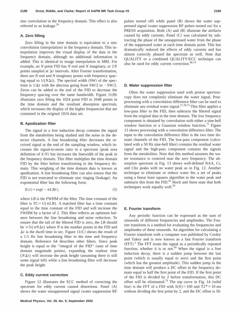
Figure 12 illustrates the ECC method of correcting tspectrum for eddy current caused distortions. Panel~A!shows the water unsuppressed signal~water suppression RF


o

he

,re

le-e--

se

e

To

ak

pulses turned off! while panel ~B! shows the water suppressed signal~water suppression RF pulses turned on! for aPRESS acquisition. Both~A! and ~B! illustrate the artifactscaused by eddy currents. Panel~C! was calculated by subtracting the phase of the unsuppressed water from the pof the suppressed water at each time domain point. Thisdramatically reduced the effects of eddy currents andalmost correctly phased the spectrum as well. Note tQUALITY or a combined QUALITY/ECC technique canalso be used for eddy current correction.48,74

D. Water suppression filter

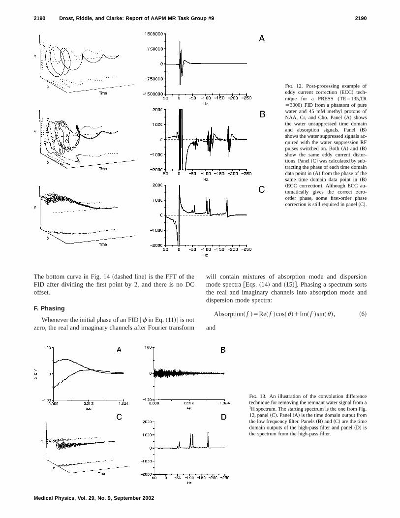
Often the water suppression used with proton spectcopy does not completely eliminate the water signal. Poprocessing with a convolution difference filter can be usedeliminate any residual water signal.27,39,75This filter applies alow-pass filter to the FID, then subtracts the filtered sigfrom the original data in the time domain. The low frequencomponent is obtained by convolution with either a sine-bwindow function or a Gaussian window function.75 Figure13 shows processing with a convolution difference filter. Tinput to the convolution difference filter is the two time dmain channels of the FID. The low-pass component~calcu-lated with a 50 Hz sine-bell filter! contains the residual watesignal and the high-pass component contains the sigfrom the metabolites. Note that this method assumes theter resonance is centered near the zero frequency. Thesorption spectrum in Fig. 13 shows well-defined NAA, Cand Cho peaks with no water peak as in Fig. 12. Anottechnique to eliminate or reduce water fits a set of peusing a linear least squares algorithm to the water peaksubtracts this from the FID.65 Hoch and Stern state that bottechniques work equally well.39

E. Fourier transform

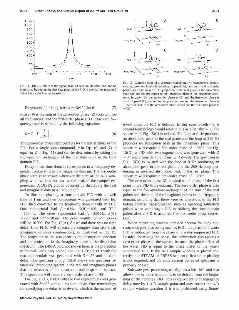
Any periodic function can be expressed as the sumsinusoids of different frequencies and amplitudes. The Frier transform is a method for evaluating the frequenciesamplitudes of these sinusoids. An algorithm for calculatinFourier transform with a computer was published by Cooand Tukey and is now known as a fast Fourier transfo~FFT!.2 The FFT treats the signal as a periodically repeafunction, whether it is or not.69 When the signal is a freeinduction decay, there is a sudden jump between thepoint ~which is usually equal to zero! and the first point~which has the greatest amplitude!. This sudden jump in thetime domain will produce a DC offset in the frequency dmain equal to half the first point of the FID. If the first poinof the FID is divided by 2 before transformation, this Doffset will be eliminated.76 The top curve in Fig. 14~solidline! is the FFT of a FID withS(0)5100 and T2* 510 mswithout dividing the first point by 2, and the DC offset is 5

f

f

in

c-F

r-

in

-se


FIG. 12. Post-processing example oeddy current correction~ECC! tech-nique for a PRESS (TE5135,TR53000) FID from a phantom of purewater and 45 mM methyl protons oNAA, Cr, and Cho. Panel~A! showsthe water unsuppressed time domaand absorption signals. Panel~B!shows the water suppressed signals aquired with the water suppression Rpulses switched on. Both~A! and ~B!show the same eddy current distotions. Panel~C! was calculated by sub-tracting the phase of each time domadata point in~A! from the phase of thesame time domain data point in~B!~ECC correction!. Although ECC au-tomatically gives the correct zeroorder phase, some first-order phacorrection is still required in panel~C!.

C

or

onsand

The bottom curve in Fig. 14~dashed line! is the FFT of theFID after dividing the first point by 2, and there is no Doffset.

F. Phasing

Whenever the initial phase of an FID@f in Eq. ~11!# is notzero, the real and imaginary channels after Fourier transf


m

will contain mixtures of absorption mode and dispersimode spectra@Eqs.~14! and ~15!#. Phasing a spectrum sortthe real and imaginary channels into absorption modedispersion mode spectra:

Absorption~ f !5Re~ f !cos~u!1Im~ f !sin~u!, ~6!

and

aig.

FIG. 13. An illustration of the convolution differencetechnique for removing the remnant water signal from1H spectrum. The starting spectrum is the one from F12, panel~C!. Panel~A! is the time domain output fromthe low frequency filter. Panels~B! and~C! are the timedomain outputs of the high-pass filter and panel~D! isthe spectrum from the high-pass filter.

th

em

dedaexa

llET

ks

uion

-ntr

-

o

sHzhis

innro-his

torealcyID

tionin

-

cur-aterID.

es aet ofer-or-ing

is

hatgin-he/De-

nre

on-

ptionpec-e ise ise is


Dispersion~ f !5Im~ f !cos~u!2Re~ f !sin~u!. ~7!

Phase~u! is the sum of the zero-order phase~Z! ~constant forall frequencies! and the first-order phase~F! ~linear with fre-quency! and is defined by the following equation:

u5Z1FS f

SWD . ~8!

The zero-order phase term corrects for the initial phase ofFID. For a single spin compound,u in Eqs. ~6! and ~7! isequal tof in Eq. ~11! and can be determined by taking thfour-quadrant arctangent of the first data point in the tidomain FID.

Delay in the time domain corresponds to a frequencypendent phase shift in the frequency domain. The first-orphase term is necessary whenever the start of the A/D spling window does not start at the peak of the dampedponential. A DISPA plot is obtained by displaying the reand imaginary data in a ‘‘XY’’ plot. 77

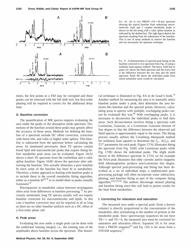
To illustrate phasing, a time domain FID with a dwetime of 1 ms and two components was generated with~11!, then converted to the frequency domain with an FFOne exponential hadf 050 Hz, S(0)5100, and T2*5100 ms. The other exponential hadf 05250 Hz, S(0)5200, and T2* 550 ms. The peak heights for both peawill be 10 000. For Fig. 15~A!, Z50° and there was no timedelay. Like FIDs, MR spectra are complex data sets~real,imaginary, or some combination!, as illustrated in Fig. 15.The projection in the real plane is the absorption spectrand the projection in the imaginary plane is the dispersspectrum.~The DISPA plot, not shown here, is the projectioin the real–imaginary plane.! For Fig. 15~B!, a FID with thetwo exponentials was generated withZ545° and no timedelay. The spectrum in Fig. 15~B! shows the spectrum rotated 45°, producing spectra in the real and imaginary plathat are mixtures of the absorption and dispersion specThis spectrum will require a zero order phase of 45°.

For Fig. 15~C!, a FID with the two exponentials was generated withZ50° and a 1 mstime delay. One terminologyfor specifying the delay is as dwells, which is the number

FIG. 14. The DC offset of the signal peak, as seen on the solid line, caeliminated by setting the first data point of the FID to one-half its measuvalue before the Fourier transform.


e

e

-erm--

l

q..

mn

esa.

f

dwell times the FID is delayed. In this case, dwells51. Asecond terminology would refer to this as a left shift51. Thespectrum in Fig. 15~C! is twisted. The loop at 0 Hz producean absorption peak in the real plane and the loop at 250produces an absorption peak in the imaginary plane. Tspectrum will require a first order phase of2360°. For Fig.15~D!, a FID with two exponentials was generated withZ50° and a time delay of 2 ms, or 2 dwells. The spectrumFig. 15~D! is twisted with the loop at 0 Hz producing aabsorption peak in the real plane and the 250 Hz loop pducing an inverted absorption peak in the real plane. Tspectrum will require a first-order phase of2720°.

The zero-order phase~Z! is equal to the phase of the firspoint in the FID~time domain!. The zero-order phase is alsequal to the four-quadrant arctangent of the sum of thepoints and the sum of the imaginary points in the frequendomain, providing that there were no alterations to the Fbefore Fourier transformation such as applying saturapulses when acquiring a FID or shifting the time domapoints after a FID is acquired~for first-order phase correction!.

When correcting water-suppressed spectra for eddyrents with post-processing such as ECC, the phase of a wFID is subtracted from the phase of a water-suppressed FBesides linearizing the phase, this subtraction also applizero-order phase to the spectra because the phase offsthe water FID is equal to the phase offset of the watsuppressed FID. If the A/D sample window is placed crectly in a STEAM or PRESS sequence, first-order phasis not required, and the eddy current corrected spectrumproperly phased.

Software post-processing usually has a left shift tool tallows one or more data points to be deleted from the bening of the complex FID. This is equivalent to changing tdelay time by 1 A/D sample point and may correct the Asample window position if it was positioned early. Som

bed

FIG. 15. Complex plots of a spectrum containing two components demstrating zero- and first-order phasing. In panel~A!, both zero- and first-orderphases are equal to zero. The projection in the real plane is the absorspectrum and the projection in the imaginary plane is the dispersion strum. In panel~B!, the zero-order phase is 45° and the first-order phaszero. In panel~C!, the zero-order phase is zero and the first-order phas2360°. In panel~D!, the zero-order phase is zero and the first-order phas2720°.

o-

ashee.

ine

e

ineed


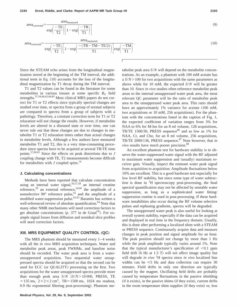
FIG. 16. An in vivo PRESS (TE530 ms) spectrumshowing the typical baseline from underlying macrmolecule, lipid andJ coupled metabolite peaks isshown on the left along with a cubic spline baselineindicated by the dashed line. The right figure depicts tspectrum resulting from the subtraction of the baselinThis is one of many methods to remove the baseland not necessarily the optimum technique.

FIG. 17. A demonstration of spectral peak fitting on thbaseline correctedin vivospectrum from Fig. 16 using anonlinear least-squares method. The heavy solid linepanel~A! shows the fitted spectrum and the lower linis the difference between the raw data and the fittspectrum. Panel~B! shows the individual peaks fromwhich metabolite areas would be calculated.

eseay

thDffeasonsethtabe6ub-

linteks

,

to

irehiloet

wheto

.lectbe-

lcu-an-

eirithofand

inghod

fit

etices.de-ost-ion,ingngfor

ehehavefor

times, the first points in a FID may be corrupted and thpoints can be removed with the left shift tool, but first-ordphasing will be required to correct for the additional deltime.

G. Baseline correction

The quantification of MR spectra requires evaluatingarea under the peaks in the absorption mode spectrum.tortions of the baseline around these peaks may greatly athe accuracy of these areas. Methods for defining the bline of a spectrum include DC offset correction, correctiwith linear tilts, and cubic or higher order splines. This baline is subtracted from the spectrum before calculatingareas. As mentioned previously, short TE spectra conbroad lipid and macromolecule peaks that require fittingfore metabolite peak areas can be evaluated. Figure 1~A!shows a short TE spectrum from the cerebellum and a cspline baseline. Figure 16~B! shows the spectrum after subtracting the baseline. This actually illustrates a poor basefit since some of the baseline has been fit to metaboliTherefore, a better approach to dealing with baseline peato include them in the overall metabolite fitting algorithmeither as a baseline fit66,78or to model them as peaks~usuallyGaussian!.67

Discrepancies in metabolite values between investigaoften arise from differences in baseline processing.78 As pre-viously mentioned, long TE spectra usually will not requbaseline correction for macromolecules and lipids. In tcase a baseline correction may not be required at all asas there are no other baseline artifacts such as a DC offsa first-order phase roll.

H. Peak areas

Evaluating the area under a single peak can be donethe traditional running integral, i.e., the running sum of tamplitudes above baseline across the spectrum. This his


er

eis-cte-

-ein-

ic

es.is

rs

sngor

ith

ri-

cal technique is illustrated in Fig. 8.6 in de Graaf’s book79

Another method for measuring the area is to manually sebaseline points under a peak, then determine the areatween this baseline and the spectral points. However, calating areas in spectra with multiple, overlapping peaks cnot be evaluated this way.80 With overlapping peaks, it isnecessary to deconvolve the individual peaks to find thareas. Such deconvolution involves fitting a spectrum wLorentzian, Gaussian, or a Lorentzian–Gaussian mixtureline shapes so that the difference between the observedfitted spectra is approximately equal to the noise. The fittprocess usually utilizes the Levenberg–Marquardt metfor nonlinear least squares to determine thef 0 , A( f 0), andT2* parameters for each peak. Figure 17~A! illustrates fittingthe spectrum from Fig. 16~B! with Lorentzian peaks whileFig. 17~B! shows the individual peaks. The slight misshown in the difference spectrum in 17~A! on for examplethe NAA peak illustrates that eddy currents and/or magnfield inhomogeneties produce non-Lorentzian line shapAlthough spectral post-processing and fitting has beenscribed as a set of individual steps, a sophisticated pprocessing package will often incorporate water subtractphasing, and baseline fitting as part of the computer fittalgorithm.65,67,81,82The authors discourage manual phasiand baseline fitting since this will lead to poorer resultsthe final fitted metabolites.

I. Correcting for relaxation and saturation

The measured area under a spectral peak~from a knownvolume! is directly proportional to the concentration of thmetabolite, after normalizing to the number of protons in tmetabolite peak. Since spectroscopy sequences do notTR5` and TE50, the measured area must be correctedsaturation and relaxation effects. Equation~9! is for areasfrom a PRESS sequence83 and Eq.~10! is for areas from aSTEAM sequence,57

areacorrected5areameasured

~9!


expS 2TE

T2 D F12expS 2TR

T1 D Gareacorrected5

areameasured

expS 2TE

T2 D F12expS 2~TR2TM2TE/2!

T1 D GexpS 2TM

T1 D . ~10!

nedi-

m

-arc

hTlitecm

gerecetim

cu

ti

t

le

edoiteuan

o

t,

-hasas

akmostakould

1,for,

s,

b-sted

nalwforc-al

atering/ard-ive.

g atredlly,Msureur.Hzte

0lyblyding

Since the STEAM echo arises from the longitudinal magtization stored at the beginning of the TM interval, the adtional term in Eq.~10! accounts for the loss of the longitudinal magnetization by T1 decay during the TM interval.

T1 and T2 values can be found in the literature for sometabolites in various tissues at some specificB0 fieldstrengths.57,59,60,62,84,85Most clinical MRS papers do not correct for T1 or T2 effects since typically spectral changesstudied over time, or spectra from a group of normal subjeare compared to spectra from a group of subjects witpathology. Therefore, a constant correction term for T1 orrelaxation will not change the results. However, if metabolevels are altered in a diseased state or over time, onenever rule out that these changes are due to changes intabolite T1 or T2 relaxation times rather than actual chanin metabolite levels. Although a few authors have measumetabolite T1 and T2, this is a very time-consuming produre since spectra have to be acquired at several TR/TEpoints.57,60,61 Since the effects on peak distortions due toJcoupling change with TE, T2 measurements become diffifor metabolites withJ coupled spins.14

J. Calculating concentrations

Methods have been reported that calculate concentrausing an internal water signal,56,57,58 an internal creatinereference,59 an external reference,54,60 the amplitude of anonselective 90° reference pulse,61 and the amplitude of amodified water-suppression pulse.62,63 Barantin has written awell-referenced review of absolute quantification.64 Note thatmany other NMR mechanisms will need correction factorsget absolute concentrations~p. 377 in de Graaf79!. For ex-ample signal losses from diffusion and nonideal slice profiwill need correction factors.

XIII. MRS EQUIPMENT QUALITY CONTROL „QC…

The MRS phantom should be measured every 1–4 wewith all the in vivo MRS acquisition techniques. Water anmetabolite peak areas, peak FWHMs, and baseline nshould be recorded. The water peak area is from a waunsuppressed acquisition. Two sequential water unspressed spectra should be acquired so that the second cused for ECC~or QUALITY ! processing on the first. Twoacquisitions for the water unsuppressed spectra provide mthan enough peak areaS/N ~S/N.10 000, PRESS, TE5135 ms, 23232 cm3, TR51500 ms, 1024 ms readou0.9 Hz exponential filtering post-processing!. Phantom me-


--

e

etsa2

ane-sd-e

lt

on

o

s

ks

ser-p-

be

re

tabolite peak areaS/N will depend on the metabolite concentrations. As an example, a phantom with 100 mM acetatea S/N.100 for two acquisitions with the same parametersabove while for 10 mM, the expectedS/N will be greaterthan 10. Sincein vivo studies often reference metabolite peareas to the internal unsuppressed water peak area, therelevant QC parameter will be the ratio of metabolite pearea to the unsuppressed water peak area. This ratio shhave an approximately 1% variance for acetate~100 mM,two acquisitions or 10 mM, 256 acquisitions!. For the phan-tom with the concentrations listed in the caption of Fig.the expected coefficient of variation ranges from 3%NAA to 6% for M-Ins for an 8 ml volume, 128 acquisitionsTR/TE 1500/30, PRESS sequence86 and as low as 1% forNAA, Cr, and Cho, for an 8 ml volume, 256 acquisitionTR/TE 2000/136, PRESS sequence.87 Note however, thatinvivo results have much poorer precision.88

An excellent phantom test for hardware stability is to oserve the water-suppressed water signal with the RF adjuto maximum water suppression and~usually! maximum re-ceiver gain. Visually, inspect the remnant water peak sigfrom acquisition to acquisition. Amplitude fluctuations belo10% are excellent. This is a good hardware test especiallylow level RF stability, but since some type of water subtration is done in1H spectroscopy post-processing, the finspectral quantification may not be affected by unstable wsuppression, as long as a sophisticated water fittsuppression routine is used in post-processing. If these hware instabilities also occur during the RF volume selectpulses and rephasing gradients, spectra will be degraded

The unsuppressed water peak is also useful for lookinoverall system stability, especially if the data can be acquiand displayed in real time in the frequency domain. Usuathis is done after performing a localized shim with a STEAor PRESS sequence. Continuously acquire data and meachanges in peak position and signal amplitude for an hoThe peak position should not change by more than 1while the peak amplitude typically varies around 1%. Nothat the typical manufacturer’s specification of,0.1 ppmfield drift ~6 Hz at 1.5 T! will not affect image quality butwill degradein vivo 1H spectra sincein vivo localized linewidths can be<5 Hz and data collection can require 3minutes. Field drifts in only one direction are typicalcaused by the magnet. Oscillating field drifts are probacaused by temperature fluctuations in the passive shiel~if it exists!, in the passive shims~if they exist!, current driftsin the room temperature shim supplies~if they exist! or, less

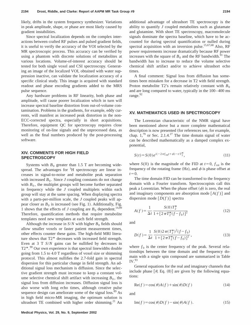
nd

teelhe

abrap

ofrR

nilloncuonnos,sin

e--tieed

ct

lit

erathinblingrad

ecvo

ils

s

theteuleac-

ng

wer

tiveho

e-gth.

ms

veticale,rex-

cyhis

la-do-ble

that-


likely, drifts in the system frequency synthesizer. Variatioin peak amplitude, shape, or phase are most likely causegradient instabilities.

Since spectral localization depends on the complex inactions between crafted RF pulses and pulsed gradient fiit is useful to verify the accuracy of the VOI selected by tMR spectroscopic process. This accuracy can be verifiedusing a phantom with discrete solutions of metabolitesvarious locations. Volume-of-interest accuracy shouldtested for both single voxel and CSI spectroscopy. Geneing an image of the localized VOI, obtained with water supression inactive, can validate the localization accuracyspecific clinical study. This image is acquired with standareadout and phase encoding gradients added to the Mpulse sequence.

Any hardware problems in RF linearity, both phase aamplitude, will cause poorer localization which in turn wincrease spectral baseline distortion from out-of-volume ctamination. Problems in the gradients, for example, eddyrents, will manifest as increased peak distortion in the nECC-corrected spectra, especially in short acquisitioTherefore, equipment QC for spectroscopy requires clmonitoring of on-line signals and the unprocessed datawell as the final numbers produced by the post-processoftware.

XIV. COMMENTS FOR HIGH FIELDSPECTROSCOPY

Systems withB0 greater than 1.5 T are becoming widspread. The advantages for1H spectroscopy are linear increases in signal-to-noise and metabolite peak separawith increasedB0 . SinceJ coupling constants do not changwith B0 , the multiplet groups will become further separatin frequency while theJ coupled multiplets within eachgroup will stay at the same spacing. When displaying spewith a parts-per-million scale, theJ coupled peaks will ap-pear closer asB0 is increased~see Fig. 1!. Additionally, Fig.1 shows that the effects ofJ coupling areB0 dependent.14,89

Therefore, quantification methods that require metabotemplates need new templates at each field strength.

Although the increase inS/N with higherB0 fields shouldallow smaller voxels or faster patient measurement timother effects counter these gains. The high-field MRI liteture shows that T2* decreases with increased field strengEven at 3 TS/N gains can be nullified by decreasesT2* .90 Our own experience is that spectral linewidths dougoing from 1.5 to 4.0 T regardless of voxel size or shimmprotocol. This almost nullifies the 2.7-fold gain in spectdispersion for this particular change in field strength. An aditional signal loss mechanism is diffusion. Since the seltive gradient strength must increase to keep a constantume selective chemical shift artifact with increasingB0 , thesignal loss from diffusion increases. Diffusion signal lossalso worse with long echo times, although creative pusequence design can ameliorate some of the signal loss.89 Asin high field micro-MR imaging, the optimum solution iultrashort TE combined with higher order shimming.21 An


sby

r-ds,

byt

et-

-a

dS

d

-r--

s.e

asg

on

ra

e

s,-.

e

l--l-

se

additional advantage of ultrashort TE spectroscopy isability to quantify J coupled metabolites such as glutamaand glutamine. With short TE spectroscopy, macromolecsignals dominate the spectra baseline, which have to becounted for during spectral quantification or nulled durispectral acquisition with an inversion pulse.15,67,68Also, RFpower requirements increase dramatically because RF poincreases with the square ofB0 and the RF bandwidth.91 Thebandwidth has to increase to reduce the volume selecchemical shift artifact and/or to achieve ultrashort ectimes.

A final comment: Signal loss from diffusion has somtimes been mistaken for a decrease in T2 with field strenProton metabolite T2’s remain relatively constant withB0

and are long compared to water, typically in the 100–400range.92

XV. MATHEMATICS USED IN SPECTROSCOPY

The Lorentzian characteristic of the NMR signal habeen mentioned above but a more complete mathemadescription is now presented~for references see, for examplchap. 1,79 or Sec. 2.1.4.27 The time domain signal of watecan be described mathematically as a damped complexponential,

S~ t !5S~0!ei ~22p f rott1f!2t/T2* , ~11!

whereS(0) is the magnitude of the FID att50, f rot is thefrequency of the rotating frame~Hz!, andf is phase offset att50.

The time domain FID can be transformed to the frequendomain with a Fourier transform. Spectroscopists call tpeak a Lorentzian. When the phase offset~f! is zero, the realand imaginary components are absorption mode@A( f )# anddispersion mode@D( f )# spectra

A~ f !51

Dt

S~0!T2*

11@2pT2* ~ f 2 f 0!#2 ~12!

and

D~ f !51

Dt

S~0!2p~T2* !2~ f 2 f 0!

11@2pT2* ~ f 2 f 0!#2 , ~13!

where f 0 is the center frequency of the peak. Several retionships between the time domain and the frequencymain with a single spin compound are summarized in TaIV.93

General equations for the real and imaginary channelsinclude phase@u, Eq. ~8!# are given by the following equations:

Re~ f !5cos~u!A~ f !1sin~u!D~ f ! ~14!

and

Im~ f !5cos~u!D~ f !2sin~u!A~ f !. ~15!

inRbnt’sui

Sonc

ubde-f ten

nd

d

n

n

bo

G

97,

in,’’

les:

-

l-e offorse-

ail:

. E.nd

on

K.ing

al

set on

led

c

um

a-fer,’’

ce

i-

n


XVI. RECOMMENDATIONS AND SUGGESTEDREADING

Expertise in MRS can best be gained from experimentwith the MRS phantom that comes with the clinical Msystem. Other experimental NMR systems may be availain Radiology and Biochemistry departments, and understaing the function of these devices will improve the physicisoverall skills in MRS. Due to the complexities of data acqsition in MRS, described above, the physicist without MRexperience must be willing to commit a significant amounttime in order to learn the subtle variances that can influethe MRS measurement.

Fortunately, there is a large body of literature on the sject of MRS. The following is a list of monographs anreview articles that the authors have found to be most gerally useful. MR Task Group # 9 would especially recommend that de Graaf’s book should be consulted as one ofirst references for all the referenced topics in this docum

Useful overviews on MRS include the following.Canet, D., Nuclear Magnetic Resonance: Concepts aMethods~Wiley, New York, 1991!.de Graaf, R. A.,In vivo NMR Spectroscopy: Principles anTechniques~Wiley, New York, 1998!.de Graaf, R. A. and Rothman D. L., ‘‘In vivo detection andquantification of scalar coupled 1H NMR resonances,’’ Cocepts Magn. Reson.13, 32–76~2001!.Frahm, J., Merbolt, K., Hanicke, W., ‘‘Localized protospectroscopy using stimulated echoes,’’ J. Magn. Reson.72,502–508~1987!.Govindaraju, V., Young, K., Maudsley, A. A., ‘‘Proton NMRchemical shifts and coupling constants for brain metalites,’’ NMR Biomed. 13, 129–153~2000!.Hoch, J. C. and Stern, A. S.,NMR Data Processing~Wiley-Liss, New York, 1996!.Howe, F. A., Maxwell, R. J., Saunders, D. E., and Brown,Jr., ‘‘Proton spectroscopyin vivo,’’ Magn. Reson. Quart.9,31–39~1993!.

TABLE IV. Mathematical relationships of a single spin compound.

Time domain Frequency domai

Initial amplitude of FID S(0)A~f0!Dt

T2*

‘‘Integral’ ’ of FID S (i 51

n

M i D S~0!T2*

DtA( f 0)

T2*Dt(i51

n Mi

S~0!

1

pFWHM

Amplitude of peak (i 51

n

M iA( f 0)

Peak area (*2`` A( f )d f )

S~0!

2Dt

A~f0!

2T2*

Full-width at half-maximum~FWHM!S~0!

pDt(i51n Mi

1

pT2*

Full-width at tenth-maximum~FWTM! 33S~0!

pDt(i51n Mi

3

pT2*


g

led-

-

fe

-

n-

het.

-

-

.

Lenkinski, R. E., MR Spectroscopy, RSNA CategoricalCourse in Physics: The Basic Physics of MR Imaging, 19pp. 163–174.Narayana, P. A. and Jackson, E. F., ‘‘Image-guidedin vivoproton magnetic resonance spectroscopy in human braCurr. Sci.61, 340–350~1991!.Riddle, W. R. and Lee, H., ‘‘Magnetic resonance: Principand spectroscopy,’’ inBiomedical Uses of Radiation, Part ADiagnostic Applications, edited by W. R. Hendee~VCH Pub-lishers, New York, 1999!, pp. 419–480.Ross, B. and Michaelis, T., ‘‘Clinical applications of magnetic resonance spectroscopy,’’ Magn. Reson. Q.10, 191–247 ~1994!.Salibi, N. and Brown, M. A.,Clinical MR Spectroscopy:First Principles ~Wiley-Liss, New York, 1998!.Sanders, J. A., ‘‘Magnetic resonance spectroscopy,’’ inFunc-tional Brain Imaging, edited by W. W. Orrison, Jr.~Mosby-Year Book, St. Louis, MO, 1995!, Chap. 10.

ACKNOWLEDGMENTS

The authors would like to thank all of our clinical coleagues that have provided input and discussion on the usMRS. We would also like to thank our graduate studentstheir work in spectral quantification and spectroscopyquence development.

a!Author to whom correspondence should be addressed. Electronic [email protected]. G. Webb, N. Sailasuta, S. J. Kohler, T. Raidy, R. A. Moats, and RHurd, ‘‘Automated single-voxel proton MRS: Technical development amultisite verification,’’ Magn. Reson. Med.31, 365–373~1994!.

2J. W. Cooley and J. W. Tukey, ‘‘An algorithm for the machine calculatiof complex Fourier series,’’ Math. Comput.19, 297–301~1965!.

3Y. Ishihara, A. Calderon, H. Watanabe, K. Okamoto, Y. Suzuki,Kuroda, and Y. Suzuki, ‘‘A precise and fast temperature mapping uswater proton chemical shift,’’ Magn. Reson. Med.34, 814–823~1995!.

4V. Govindaraju, K. Young, and A. A. Maudsley, ‘‘Proton NMR chemicshifts and coupling constants for brain metabolites,’’ NMR Biomed.13,129–153~2000!.

5N. Salibi and M. A. Brown,Clinical MR Spectroscopy: First Principles~Wiley-Liss, New York, 1998!.

6R. B. Thompson and P. S. Allen, ‘‘Sources of variability in the responof coupled spins to the PRESS sequence and their potential impacmetabolite quantification,’’ Magn. Reson. Med.41, 1162–1169~1998!.

7R. B. Thompson and P. S. Allen, ‘‘Response of metabolites with coupspins to the STEAM sequence,’’ Magn. Reson. Med.45, 955–965~2001!.

8T. H. Ernst and J. Hennig, ‘‘Coupling effects in volume selective1Hspectroscopy of major brain metabolites,’’ Magn. Reson. Med.21, 82–96~1991!.

9P. S. Allen, R. B. Thompson, and A. H. Wilman, ‘‘Metabolite-specifiNMR spectroscopyin vivo,’’ NMR Biomed. 10, 435–444~1997!.

10J. R. Keltner, L. L. Wald, B. D. Frederick, and P. F. Renshaw, ‘‘In vivodetection of GABA in human brain using a localized double-quantfilter technique,’’ Magn. Reson. Med.37, 366–371~1997!.

11H. Lei and J. Peeling, ‘‘Simultaneous spectral editing for gammaminobutyric acid and taurine using double quantum coherence transJ. Magn. Reson.143, 95–100~2000!.

12B. Ross and T. Michaelis, ‘‘Clinical applications of magnetic resonanspectroscopy,’’ Magn. Reson. Q.10, 191–247~1994!.

13E. R. Danielsen and B. D. Ross,Magnetic Resonance Spectroscopy Dagnosis of Neurological Diseases~Marcel Dekker, New York, 1999!.

14R. A. de Graaf and D. L. Rothman, ‘‘In vivo detection and quantificationof scalar coupled 1H NMR resonances,’’ Concepts Magn. Reson.13,32–76~2001!.

ff,

e

py

nt-

ing

H

s-

th

eti, p

er,n

ly,

n,s-

.,’’

nJ.

ceu-

Ded

igati

A.bonc

fn

onma

ifi-

eti

p.

ign

le

,e

ew

ta,-

ent

ian

s,’’

y

veSoc.

A.s:ra-

ndgn.

etic

ews,anMR

ofrnal

. W.g

heral

ndgn.

Rulse:

ali-


15K. L. Behar, D. L. Rothman, D. D. Spencer, and O. A. C. Petro‘‘Analysis of macromolecule resonances in1H NMR spectra of humanbrain,’’ Magn. Reson. Med.32, 294–302~1994!.

16U. Seeger, I. Mader, T. Nagele, W. Grodd, O. Lutz, and U. Klose, ‘‘Rliable detection of macromolecules in single-volume1H NMR spectra ofthe human brain,’’ Magn. Reson. Med.45, 948–954~2001!.

17J. Frahm, K. Merbolt, and W. Hanicke, ‘‘Localized proton spectroscousing stimulated echoes,’’ J. Magn. Reson.72, 502–508~1987!.

18P. A. Bottomley, ‘‘Spatial localization in NMR spectroscopyin vivo,’’Ann. N.Y. Acad. Sci.508, 333–348~1987!.

19W. R. Riddle, S. J. Gibbs, and M. R. Wilcott, ‘‘Dissecting and implemeing STEAM spectroscopy,’’ Magn. Reson. Med.29, 378–380~1993!.

20J. Frahm, H. Bruhn, M. L. Gyngell, K. D. Merboldt, W. Ha¨nicke, and R.Sauter, ‘‘Localized high-resolution proton NMR spectroscopy usstimulated echoes: Initial applications to human brainin vivo,’’ Magn.Reson. Med.9, 79–93~1989!.

21I. Tkac, Z. Starcuk, I.-Y. Choi, and R. Gruetter, ‘‘In vivo 1H NMR spec-troscopy of rat brain at 1 ms echo time,’’ Magn. Reson. Med.41, 649–656 ~1999!.

22T. Ernst and L. Chang, ‘‘Elimination of artefacts in short echo time 1MR spectroscopy of the frontal lobe,’’ Magn. Reson. Med.36, 462–468~1996!.

23C. T. W. Moonen and P. C. M. van Zijl, ‘‘Highly effective water suppresion for in vivo proton NMR spectroscopy,’’ J. Magn. Reson.88, 28–41~1990!.

24I. Tkac, E. R. Seaquist, and R. Gruetter, ‘‘A comparison of several meods for quantification of resolved glucose signals in1H NMR spectra ofthe human brain,’’ Proceedings of the International Society for MagnResonance in Medicine, 8th Meeting, Denver, Colorado, 2000, Vol. 31938.

25I. Tkac, P. Anderson, G. Adriany, H. Merkle, K. Ugurbil, and R. Gruett‘‘ In vivo 1H NMR spectroscopy of the human brain at 7T,’’ Magn. ResoMed. 46, 451–456~2001!.

26C. T. Moonen, M. von Kienlin, P. C. van Zijl, J. Cohen, J. Gillen, P. Daand G. Wolf, ‘‘Comparison of single-shot localization methods~STEAMand PRESS! for in vivo proton NMR spectroscopy,’’ NMR Biomed.2,201–208~1989!.

27D. Canet,Nuclear Magnetic Resonance: Concepts and Methods~Wiley,New York, 1991!.

28D. A. Yablonskiy, J. J. Neil, M. E. Raichle, and J. J. H. Ackerma‘‘Homonuclear J coupling effects in volume localized NMR spectrocopy: pitfalls and solutions,’’ Magn. Reson. Med.39, 169–178~1998!.

29J. H. Duyn, J. Gillen, G. Sobering, P. C. M. van Zijl, and C. T. WMoonen, ‘‘Multisection proton MR spectroscopy imaging of the brainRadiology188, 277–282~1993!.

30C. T. W. Moonen, G. Sobering, P. C. M. Van Zijl, J. Gillen, M. VoKienlin, and A. Bizzi, ‘‘Proton spectroscopic imaging of human brain,’’Magn. Reson.98, 556–575~1992!.

31T. R. Brown, B. M. Kincaid, and K. Ugurbil, ‘‘NMR chemical shiftimaging in three dimensions,’’ Proc. Natl. Acad. Sci. U.S.A.79, 3523–3526 ~1982!.

32D. C. Shungu and J. D. Glickson, ‘‘Sensitivity and localization enhanment in multinuclearin vivo NMR spectroscopy by outer volume presatration,’’ Magn. Reson. Med.30, 661–671~1993!.

33E. Adalsteinsson, P. Irarrazabal, S. Tropp, C. Meyer, A. Macovski, andM. Spielman, ‘‘Volumetric spectroscopic imaging with spiral-bask-space trajectories,’’ Magn. Reson. Med.39, 889–898~1998!.

34S. Posse, G. Tedeschi, R. Risinger, R. Ogg, and D. Le Bihan, ‘‘Hspeed 1H spectroscopic imaging in human brain by echo planar spspectral encoding,’’ Magn. Reson. Med.33, 34–40~1995!.

35N. Schuff, F. Ezekiel, A. C. Gamst, D. L. Amend, A. A. Capizzano, A.Maudsley, and M. W. Weiner, ‘‘Region and tissue differences of metalites in normally aged brain using multislice 1H magnetic resonaspectroscopic imaging,’’ Magn. Reson. Med.45, 899–907~2001!.

36C. I. Haupt, N. Schuff, M. W. Weiner, and A. A. Maudsley, ‘‘Removal olipid artifacts in 1H spectroscopic imaging by data extrapolation,’’ MagReson. Med.35, 678–687~1996!.

37X. Golay, J. Gillen, P. C. van Zijl, and P. B. Barker, ‘‘Scan time reductiin proton magnetic resonance spectroscopic imaging of the hubrain,’’ Magn. Reson. Med.47, 384–387~2002!.

38R. Bartha, D. J. Drost, and P. C. Williamson, ‘‘Comparing the quantcation of single volume and CSI short echo STEAM1H spectra in the leftbasal ganglia,’’ Proceedings of the International Society for Magn


-

-

c.

.

-

.

hal-

-e

.

n

c

Resonance in Medicine, 4th meeting, New York, NY, 1996, Vol. 2,1182.

39J. C. Hoch and A. S. Stern,NMR Data Processing~Wiley-Liss, NewYork, 1996!.

40E. M. Haacke, R. W. Brown, M. R. Thompson, and R. Venkatesan,Mag-netic Resonance Imaging: Physical Principles & Sequence Des~Wiley-Liss, New York, 1999!, Sec. 15.2.

41I. S. Mackenzie, E. M. Robinson, A. N. Wells, and B. Wood, ‘‘A simpfield map for shimming,’’ Magn. Reson. Med.5, 262–268~1987!.

42D. M. Doddrell, G. L. Galloway, I. M. Brereton, and W. M. Brooks‘‘Nodal inhomogeneity mapping by localized excitation—th‘‘NIMBLE’’ shimming technique for high-resolutionin vivo NMR spec-troscopy,’’ Magn. Reson. Med.7, 352–357~1988!.

43M. G. Prammer, J. C. Haselgrove, M. Shinnar, and J. S. Leigh, ‘‘A napproach to automatic shimming,’’ J. Magn. Reson.77, 40–52~1988!.

44J. Tropp, K. A. Derby, C. Hawryszko, S. Sugiura, and H. Yamaga‘‘Automated shimming ofB0 for spectroscopic imaging,’’ J. Magn. Reson.85, 244–254~1989!.

45P. Webb and A. Macovski, ‘‘Rapid, fully automatic, arbitrary-volumeinvivo shimming,’’ Magn. Reson. Med.19, 113–122~1991!.

46R. Gruetter, ‘‘Automatic localizedin vivo adjustment of all first- andsecond-order shim coils,’’ Magn. Reson. Med.29, 804–811~1993!.

47M. Terpstra, P. M. Andersen, and R. Gruetter, ‘‘Localized eddy currcompensation using quantitative field mapping,’’ J. Magn. Reson.131,139–143~1998!.

48A. A. de Graaf, J. E. van Dijk, and W. M. M. J. Bovee, ‘‘QUALITY:quantification improvement by converting lineshapes to the lorentztype,’’ Magn. Reson. Med.13, 343–357~1990!.

49U. Klose, ‘‘In vivo proton spectroscopy in presence of eddy currentMagn. Reson. Med.14, 26–30~1990!.

50W. R. Riddle, S. J. Gibbs, and M. R. Willcott, ‘‘Removing effects of eddcurrents in proton MR spectroscopy,’’ Med. Phys.19, 501–510~1992!.

51D. I. Hoult and R. E. Richards, ‘‘Critical factors in the design of sensitihigh resolution nuclear magnetic resonance spectrometers,’’ Proc. R.London, Ser. A344, 311–340~1975!.

52P. C. M. Van Zijl, C. T. W. Moonen, J. R. Alger, J. S. Cohen, and S.Chesnick, ‘‘High field localized proton spectroscopy in small volumeGreatly improved localization and shimming using shielded strong gdients,’’ Magn. Reson. Med.10, 256–265~1989!.

53J. Hennig, ‘‘The application of phase rotation for localizedin vivo spec-troscopy with short echo times,’’ J. Magn. Reson.96, 40–49~1992!.

54T. Ernst, R. Kreis, and B. D. Ross, ‘‘Absolute quantitation of water ametabolites in the human brain: I: Compartments and water,’’ J. MaReson., Ser. B102, 1–8 ~1993!.

55P. J. Hore, ‘‘Solvent suppression in Fourier transform nuclear magnresonance,’’ J. Magn. Reson.55, 283–300~1983!.

56P. B. Barker, B. J. Soher, S. J. Blackband, J. C. Chatham, V. P. Mathand R. N. Bryan, ‘‘Quantitation of proton NMR spectra of the humbrain using tissue water as an internal concentration reference,’’ NBiomed.6, 89–94~1993!.

57B. J. Soher, R. E. Hurd, N. Sailasuta, and P. B. Barker, ‘‘Quantitationautomated single-voxel proton MRS using cerebral water as an intereference,’’ Magn. Reson. Med.36, 335–339~1996!.

58P. Christiansen, O. Henriksen, M. Stubgaard, P. Gideon, and H. BLarsson, ‘‘In vivo quantification of brain metabolites by 1H-MRS usinwater as an internal standard,’’ Magn. Reson. Imaging11, 107–118~1993!.

59J. Frahm, H. Bruhn, M. L. Gyngell, K. D. Merboldt, W. Ha¨nicke, and R.Sauter, ‘‘Localized proton NMR spectroscopy in different regions of thuman brainin vivo. Relaxation times and concentrations of cerebmetabolites,’’ Magn. Reson. Med.11, 47–63~1989!.

60R. Kreis, T. Ernst, and B. D. Ross, ‘‘Absolute quantitation of water ametabolites in the human brain. II. Metabolite concentrations,’’ J. MaReson., Ser. B102, 9–19~1993!.

61T. Michaelis, K. D. Merboldt, H. Bruhm, W. Ha¨nicke, and J. Frahm,‘‘Absolute concentrations of metabolites in the adult human brainin vivo:Quantification of localized proton MR spectra,’’ Radiology187, 219–227~1993!.

62E. R. Danielsen and O. Henriksen, ‘‘Absolute quantitative proton NMspectroscopy based on the amplitude of the local water suppression pQuantification of brain water and metabolites,’’ NMR Biomed.7, 311–318 ~1994!.

63E. R. Danielsen, T. Michaelis, and B. D. Ross, ‘‘Three methods of c

r.

th-

roag

ca

hek

me

fiton

nti

rovo

e-a,

gn

ng

es

ndt,

veon.

-

led.

i-peakon.

ofas in

nge

on

Rn.

ri-

and

ros-s


bration in quantitative proton MR spectroscopy,’’ J. Magn. Reson., Se106, 287–291~1995!.

64L. Barantin and S. Akoka, ‘‘An overview of absolute quantification meods for in vivo MRS,’’ J. Magn. Reson. Anal.3, 21–27~1997!.

65H. Barkhuijsen, R. de Beer, W. M. M. J. Bove´e, and D. van Ormondt,‘‘Retrieval of frequencies, amplitudes, damping factors, and phases ftime-domain signals using a linear least-squares procedure,’’ J. MReson.61, 465–481~1985!.

66S. W. Provencher, ‘‘Estimation of metabolite concentrations from lolised in vivo proton NMR spectra,’’ Magn. Reson. Med.30, 672–679~1993!.

67R. Bartha, D. J. Drost, and P. C. Williamson, ‘‘Factors affecting tquantification of short echoin vivo 1H spectra: Prior knowledge, peaelimination, filtering,’’ NMR Biomed.12, 205–216~1999!.

68S. D. Mierisova, A. van den Boogaart, I. Tka´c, P. Van Hecke, L. Van-hamme, and T. Liptaj, ‘‘New approach for quantitation of short echo tiin in vivo 1H NMR spectra of brain using AMARES,’’ NMR Biomed.11,32–39~1998!.

69R. N. Bracewell,The Fourier Transform and Its Applications~McGraw-Hill, New York, 1978!, p. 362.

70E. O. Brigham,The Fast Fourier Transform and Its Applications~Pren-tice Hall, Englewood Cliffs, NJ, 1988!, p. 172.

71J. Slotboom, C. Boesch, and R. Kreis, ‘‘Versatile frequency domainting using time domain models and prior knowledge,’’ Magn. ResMed. 39, 899–911~1998!.

72MRUI ~Magnetic Resonance User Interface!, available at www.m-rui.uab.es

73P. V. Hecke and S. V. Huffel, ‘‘Special Issue: NMR spectroscopy quatation,’’ NMR Biomed.14, 223–283~2001!.

74R. Bartha, D. J. Drost, R. S. Menon, and P. C. Williamsom, ‘‘Spectscopic lineshape correction by QUECC: combined QUALITY deconlution and ECC correction,’’ Magn. Reson. Med.44, 641–645~2000!.

75D. Marion, M. Ikura, and A. Bax, ‘‘Improved solvent suppression in onand two-dimensional NMR spectra by convolution of time-domain datJ. Magn. Reson.64, 425–430~1989!.

76G. Otting, H. Widmer, G. Wagner, and K. Wu¨thrich, ‘‘Origin of t1 andt2

ridges in 2D NMR spectra and procedures for suppression,’’ J. MaReson.66, 187–193~1986!.

77A. G. Marshall and F. R. Verdun,Fourier Transforms in NMR, Optical,and Mass Spectroscopy~Elsevier Science, Amsterdam, 1990!, pp. 11–12,54–55, 86.

78B. J. Soher, K. Young, and A. A. Maudsley, ‘‘Representation of strobaseline contributions in1H MR spectra,’’ Magn. Reson. Med.45, 966–972 ~2001!.

79R. A. de Graaf,In vivo NMR Spectroscopy: Principles and Techniqu~Wiley, New York, 1998!.


B

mn.

-

-.

-

--

’’

.

80P. A. Bottomley, ‘‘The trouble with spectroscopy papers,’’ Radiology181,344–350~1991!.

81D. Spielman, P. Webb, and A. Macovski, ‘‘A statistical framework forinvivo spectroscopic imaging,’’ J. Magn. Reson.79, 66–77~1988!.

82J. W. C. van der Veen, R. de Beer, P. R. Luyten, and D. van Ormo‘‘Accurate quantification ofin vivo 31P NMR signals using the variableprojection method and prior knowledge,’’ Magn. Reson. Med.6, 92–98~1988!.

83B. J. Soher, P. C. M. van Zijl, J. H. Duyn, and P. B. Barker, ‘‘Quantitatiproton MR spectroscopy imaging of the human brain,’’ Magn. ResMed. 35, 356–363~1996!.

84R. E. Lenkinski, ‘‘MR spectroscopy,’’RSNA Categorical Course in Physics: The Basic Physics of MR Imaging~RSNA, Oak Brook, IL, 1997!.

85R. Kreis, ‘‘Quantitative localized1H MR spectroscopy for clinical use,’’Prog. Nucl. Magn. Reson. Spectrosc.31, 155–195~1997!.

86T. Schirmer and D. P. Auer, ‘‘On the reliability of quantitative clinicamagnetic resonance spectroscopy of the human brain,’’ NMR Biom13, 28–36~2000!.

87A. Simmons, M. Smail, E. Moore, and S. C. R. Williams, ‘‘Serial precsion of metabolite peak area ratios and water referenced metaboliteareas in proton MR spectroscopy of the human brain,’’ Magn. ResImaging16, 319–330~1998!.

88J. M. Wardlaw, D. F. Signorini, and I. Marshall, ‘‘Re: Serial precisionmetabolite peak area ratios and water referenced metabolite peak areproton MR spectroscopy of the human brain, Simmonset al. 1996, Vol.16, pages 319–330 1998,’’ Magn. Reson. Imaging17, 483–487~1999!.

89J. Hennig, T. Thiel, and O. Speck, ‘‘Improved sensitivity to overlappimultiplet signals inin vivo proton spectroscopy using a multiecho volumselective ~CPRESS! experiment,’’ Magn. Reson. Med.37, 816–820~1997!.

90P. B. Barker, D. O. Hearshen, and M. D. Boska, ‘‘Single-voxel protMRS of the human brain at 1.5 T and 3.0 T,’’ Magn. Reson. Med.45,765–769~2001!.

91D. I. Hoult, C.-N. Chen, and V. J. Sank, ‘‘The field dependence of NMimaging: II. Arguments concerning an optimal field strength,’’ MagReson. Med.3, 730–746~1986!.

92S. Michaeli, M. Garwood, XH. Zhu, L. DelaBarre, P. Andersen, G. Adany, H. Merkle, K. Ugurbil, and W. Chen, ‘‘Proton T~2! relaxation studyof water, N-acetylaspartate, and creatine in human brain using HahnCarr–Purcell spin echoes at 4 T and 7 T,’’ Magn. Reson. Med.47, 629–633 ~2002!.

93W. R. Riddle and H. Lee, ‘‘Magnetic Resonance Principles and Spectcopy,’’ in Biomedical Uses of Radiation, Part A: Diagnostic Application~VCH Publishers, New York, 1999!, pp. 419–480.

Documents

Proton magnetic resonance spectroscopy in the brain: Report of