UNIVERSITY OF NAIROBI

TITLE: GSM FREQUENCY PLANNING

PROJECT NUMBER- PRJ070

BY

NAME: MUTONGA JACKSON WAMBUA

REG NO: F17/2098/2004

SUPERVISOR: DR. CYRUS WEKESA

EXAMINER: DR. MAURICE MANG’OLI

Project report submitted in partial fulfilment of the requirement for the award of the degree of Bachelor of Science in Electrical and Electronic Engineering of the University of Nairobi.

Date of Submission: MAY 2009

DEPARTMENT OF ELECTRICAL AND INFORMATION ENGINEERING

Dedication

I dedicate this project to my parents, Timothy and Ruth, my brothers and sisters for

believing in me and standing by me all through my life. Without you I would not be what

I am today.

  ii

Acknowledgements

This undergraduate project was done at the Department of Electrical and Information

Engineering, University of Nairobi, between November 2008 and May 2009. To begin

with I would like to thank my supervisor for this project Dr. Cyrus Wekesa for all the

help and support during my work. He not only supervised and guided every development

of this project but also accorded me his own material and moral support. I am greatly

indebted to his selfless sacrifice.

Big thanks to Abraham Nyete and Eng. Fwamba, both of Safaricom Kenya Limited, for

their assistance which was invaluable. It was of great help and inspired me to put extra

hours of work into this project. I would also like to thank my friend Paul Musau for

helping me with ideas and proof reading this project report.

Last but not least I would like to thank my family and all my friends for the support

during all my studies. It would not have been possible to manage everything without you.

  iii

Abstract

Frequency planning is one of the most expensive aspects of deploying a cellular network.

If a set of base stations can be deployed with minimal service and planning, the cost of

both deploying and maintaining the network will decrease. This project explores the

automatic frequency planning problem and proposes a cost effective frequency reuse

strategy. This development is considered for a frequency and time division multiple

access (FDMA and TDMA) system i.e. GSM with a limited number of frequency bands

that requires different frequency allocations for each base station to mitigate co-channel

interference. A channel allocation algorithm is proposed which includes a channel

acquisition and a channel selection scheme. The proposed distributed dynamic channel

allocation algorithm is based on resource-planning model, where a borrower need not to

receive replies from every interfering neighbor, it can borrow a channel from that

neighbor whose all group members replies with common free channels first. The

proposed algorithm makes efficient reuse of channels and evaluates the performance in

terms of blocking probability.

 

 

 

 

 

 

 

 

 

 

 

 

  iv

Contents

Dedication……………………………………………………………………………..ii

Acknowledgements……………………………………………………………………iii

Abstract………………………………………………………………………………...iv

Acronyms used………………………………………………………………………..vii

List of figures…………………………………………………………………………..ix

1 INTRODUCTION 1

1.1 Overview………………………………………………………………………….1

1.2 Objective………………………………………………………………………….2

1.3 Outline……………………………………………………………………………2

2 BACKGROUND 4

2.1 Shared Medium Schemes………………………………………………………..4

2.1.1 FDMA…………………………………………………………………….4

2.1.2 TDMA……………………………………………………………………5

2.1.3 CDMA……………………………………………………………………6

2.1.4 SDMA…………………………………………………………………….7

2.2 Introduction to GSM Networks…………………………………………………7

2.2.1 Entities within a GSM Network………………………………………….9

2.2.2 The Radio Interface………………………………………………………12

2.2.3 Channel Structure………………………………………………………...13

3 FREQUENCY PLANNING 15

3.1 Radio Network Planning…………………………………………………………15

3.1.1 The Automatic Frequency Planning (AFP) Problem……………………..16

3.1.2 The Cellular Concept and Frequency Reuse……………………………...18

3.1.3 Selection of Frequency Reuse Patterns……………………………………19

  v

3.2 The Mobile Environment and Interference………………………………………21

3.2.1 Adjacent Channel Interference……………………………………………23

3.2.2 Co-channel Interference…………………………………………………..24

3.2.3 Methods of Reducing Co-channel Interference…………………………...25

3.2.4 Path Loss…………………………………………………………………..27

3.3 Channel Assignment strategies………………………………………………….....28

3.3.1 Fixed Channel Allocation (FCA)...………………………………………..29

3.3.2 Dynamic Channel Allocation (DCA)……………………………………...29

3.3.3 Hybrid Channel Allocation (HCA)………………………………………..31

4 PROPOSED FREQUENCY REUSE STRATEGY 33

4.1 The Frequency Reuse Pattern……………………………………………………..33

4.2 System Model……………………………………………………………………..34

4.3 The Proposed Algorithm ………………………………………………………….36

4.4 Explanation of the Algorithm……………………………………………………..40

5 SIMULATION RESULTS AND ANALYSIS 41

5.1 Description of Results……………………………………………………………..41

5.2 Analysis……………………………………………………………………………43

6 CONCLUSIONS AND RECOMMENDATIONS 44

6.1 Conclusions of the Results…………………………………………………………44

6.2 Future Development………………………………………………………………..44

7 REFERENCES AND APPENDICES 45

References …………………………………………………………………………….45

Appendices…………………………………………………………………………….46

  vi

ACRONYMS USED

GSM Global System for Mobile Communications

BTS/BS Base Transceiver Station / Base Station

MA Multiple Access

FDMA Frequency Division multiple Access

TDMA Time Division Multiple Access

CDMA Code Division Multiple Access

SDMA Space Division Multiple Access

SMS Short message Service

MHZ Mega Hertz

kHZ Kilo Hertz

MS Mobile Station

SIM Subscriber Identity Module

BSIC Base Station Identity Code

BSC Base Station Controller

BSS Base Station Subsystem

MSC Mobile Switching Centre

VLR Visitor Location Register

HLR Home Location Register

AuC Authentication Centre

EIR Equipment Identity Register

TCH/F Traffic Channel/ Full rate

TCH/H Traffic Channel/ Half rate

BCCH Broadcast Control Channel

FCC Frequency Correction Channel

RACH Random Access Channel

  vii

PCH Paging Channel

AGCH Access Grant Channel

SCH Synchronization Channel

AFP Automatic Frequency Planning

TRX Transceiver

FCA Fixed Channel Allocation

DCA Dynamic Channel Allocation

HCA Hybrid Channel Allocation

BCO Borrowing with Channel Ordering

BDCL Borrowing with Directional Channel Locking

SINR Signal to Interference Noise Ratio

AWGN Additive White Gaussian Noise

DTX Discontinuous Transmission

  viii

LIST OF FIGURES

Figure Page

2.1 FDMA……………………………………………………4

2.2 TDMA……………………………………………………5

2.3 CDMA……………………………………………………6

2.4 GSM900 Channels……………………………………….8

2.5 A portion of the GSM framing structure…………………9

2.6 Outline of the GSM Network Architecture……………..10

2.7 FDMA-TDMA………………………………………….12

2.8 Frequency band allocations……………………………..12

3.1 Radio Network Planning Process……………………….16

3.2 An example of GSM Network…………………………..17

3.3 7-cell cluster……………………………………………..19

3.4 Adjacent channel interference……………………………23

4.1 The cellular system model……………………………….36

4.2 Defining cell neighbours ………………………………...37

4.3 Sectorised system model…………………………………37

4.4 Flow chart of the channel allocation algorithm……….....39

5.1 Blocking probability graph……………………………....42

A1 Hexagonal Geometry………………………………….....46

A2 Coordinates for hexagonal geometry……………………47

  ix

   

  1

CHAPTER ONE

INTRODUCTION

1.1 Overview

Cellular mobile networks such as GSM are made up of cells, each indicating a coverage zone

with a base transceiver station (BTS) either in the center of the cell or at the corner

boundaries. A hexagon is used to represent a single cell as it would make network diagrams

tidier and that it is closest to the ideal cell shape of a circle. Each BTS (in a cluster) is

allocated a different carrier frequency and each cell has a usable bandwidth associated with

this carrier. Because only a finite part of the radio spectrum is allocated to cellular radio, the

number of carrier frequencies available is limited. This means that it is necessary to re-use the

available frequencies many times in order to provide sufficient channels for the required

demand. This introduces the concept of frequency re-use and with it the possibility of

interference between cells using the same carrier frequencies.

With a fixed number of carrier frequencies available, the capacity of the system can be

increased only by re-using the carrier frequencies more often. This means making the cell

sizes smaller. This has two basic consequences:

a) It increases the likelihood of interference (co-channel interference) between cells

using the same frequency.

b) If a mobile station is moving, it will cross cell boundaries more frequently when the

cells are small. Whenever a mobile crosses a cell boundary it must change from the

carrier frequency of the cell which it is leaving to the carrier frequency of the cell to

which it is entering, a process called handover. It cannot be performed

instantaneously and hence there will be a loss of communication while the handover

is being processed. If the cell sizes become very small handovers may occur at a very

rapid rate.

Thus GSM frequency planning is a major issue in the design of a cellular system which must

achieve an acceptable compromise between the efficient utilization of the available radio

spectrum and the problems associated with frequency re-use.

GSM is one of the fastest growing cellular communication systems in the world. The large

numbers of users, increasing usage of mobile services as well as new services force operators

   

  2

to increase the capacity offered by the networks. In many of the cellular systems, increasing

the capacity means increasing the available bandwidth and using more efficient planning of

the deployment of the base stations. Common ways to increase the capacity are the use of

smaller cells, sectorization of the cells and better assignment of frequencies to mitigate

intercellular interferences. Smaller cells increase the cost of deploying the network. This is

because this scenario requires more base stations and the network requires more planning in

the deployment and frequency assignment. The main concept of cellular communication is

the use of small low-power transmitters and frequencies that can be reused in as small

geographic areas as possible. The frequency reuse will be a key aspect in this project.

1.2 Objective of project

When designing a mobile network there are many things one needs to consider. One of these

is the frequency planning, crucial in a FDMA system. This becomes an important challenge

as the cell sizes decreases. Frequency planning takes lot of time for the operator, especially

when using small cells and it is costly. Even though the planning is expensive, it is very

essential because buying licensed frequencies and bandwidth is even more expensive. So, the

operator wants the best frequency reuse, with as little effort in management as possible, and

at low cost. A frequency planning scheme that has the same frequency reuse factor but

minimal co-channel interference and maintenance cost would be very valuable. The objective

of this project was to develop a strategy to facilitate a cost-effective frequency reuse in GSM

networks.

1.3 Outline

This project report is organized as follows;

Chapter two gives a theoretical background of GSM systems which includes shared medium

schemes, entities within a GSM network, the radio interface and channel structure.

Chapter three discusses the frequency planning procedure, the automatic frequency planning

problem, the cellular concept and frequency reuse, the mobile environment including

interferences and path loss, and the different channel assignment strategies.

In chapter four, a frequency reuse strategy is proposed and theoretical analysis presented.

System model is developed and the proposed strategy represented in form of an algorithm

and a flow chart.

   

  3

Chapter five analyses and gives a detailed discussion of the results obtained, which are

represented in form of a table and a graph. These results show a way that frequency planning

can be solved in a less expensive fashion. It is understood that a real deployment of such a

system would require more extensive tuning of the algorithm. It is hoped that an operator

could expand this to an actual network.

In chapter six conclusions and suggestions for future work are given.

At the end of this project report a list of references used is given and also appendices on the

fundamentals of cellular geometry and simulation pseudocode and Matlab code for the

proposed algorithm.

   

  4

CHAPTER TWO

BACKGROUND Below is a brief introduction to different kinds of multiple access (MA) schemes using a

shared medium. A brief description of GSM is also given to the extent of what is needed for

understanding this report.

2.1 Shared Medium Schemes There are many different ways to divide the shared medium to get multiple user access. In

this chapter, three basic types of medium division protocols are described. These are

frequency division multiple access (FDMA), time division multiple access (TDMA) and code

division multiple access (CDMA). FDMA and TDMA are explained since they are the

protocols used in GSM. CDMA is a protocol used in 3G wireless networks. The knowledge

of these three protocols will help in understanding GSM and the solution proposed in this

report.

2.1.1 FDMA

Frequency Division Multiple Access (FDMA) subdivides the available medium into a set of

narrow bandwidth channels to be shared among different users. In the example in Figure 2.1

channel 1 has been split up in 6 equally large channels. There is no need for the channels to

be equally wide. When the medium is split up, there is no restriction in assigning one user

more frequency slots in order to give him higher capacity.

Fig 2.1 FDMA

   

  5

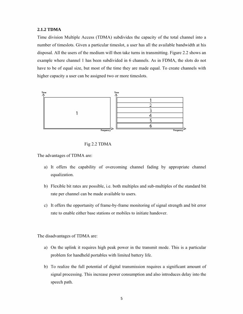
2.1.2 TDMA

Time division Multiple Access (TDMA) subdivides the capacity of the total channel into a

number of timeslots. Given a particular timeslot, a user has all the available bandwidth at his

disposal. All the users of the medium will then take turns in transmitting. Figure 2.2 shows an

example where channel 1 has been subdivided in 6 channels. As in FDMA, the slots do not

have to be of equal size, but most of the time they are made equal. To create channels with

higher capacity a user can be assigned two or more timeslots.

Fig 2.2 TDMA

The advantages of TDMA are:

a) It offers the capability of overcoming channel fading by appropriate channel

equalization.

b) Flexible bit rates are possible, i.e. both multiples and sub-multiples of the standard bit

rate per channel can be made available to users.

c) It offers the opportunity of frame-by-frame monitoring of signal strength and bit error

rate to enable either base stations or mobiles to initiate handover.

The disadvantages of TDMA are:

a) On the uplink it requires high peak power in the transmit mode. This is a particular

problem for handheld portables with limited battery life.

b) To realize the full potential of digital transmission requires a significant amount of

signal processing. This increase power consumption and also introduces delay into the

speech path.

   

  6

2.1.3 CDMA

The Code Division Multiple Access (CDMA) protocol does not split up the available medium

in terms of frequency or time. Instead all transmissions over-lap, and the correct data is

identified by a unique identification code at the receiver and the transmitter. CDMA is a form

of Direct Sequence Spread Spectrum communications. This means that the digital data x(n) is

coded at a much higher frequency. The code that is applied to the data is pseudo-random,

which means that it is constructed in a deterministic fashion, and therefore reproducible, but

such that the final code will appear random. At the receiver the same code is correlated to the

received signal to extract the data. There are three key points that explains CDMA.

a) The bandwidth is spread using a code that is independent of the data.

b) The receiver uses a code that, synchronized to the received signal, will extract the

received data. First of all, because of the code being independent from all other codes

it will allow multiple users to access the same frequencies at the same time. And

second, since the codes are pseudo-random all the data transmitted by other units,

than the two communicating with each other, will look like noise.

c) With this modulation the signal occupies a bandwidth that is much wider than

necessary to transmit the data. Because of this, one will receive a couple of benefits

such as greater tolerance against interference and disturbance on specific frequencies.

It is possible, by using CDMA, to overlay GSM with an access scheme with high

tolerance to noise and that does not add much interference to the existing system.

Fig 2.3 CDMA

   

  7

2.1.4 SDMA

Space division multiple access (SDMA) is used in all cellular communication systems. The

idea behind SDMA is allowing multiple cells to use the same radio frequency channels. For

this multiple access scheme to work it requires that the users are separated sufficiently far

apart to minimize the co-channel interference. The distance the frequencies can be separated

with is called the reuse distance. Larger distance demands usage of more frequencies. With

frequency planning this distance is made sufficiently large with as few frequencies as

possible. This will be one of the main issues in this project.

2.2 Introduction to GSM Networks Throughout the evolution of cellular communications, many different systems have been

developed apart from each other, resulting in huge problems when it came to compatibility.

The GSM was developed with this in mind and intended to solve these problems. GSM was

the first digital communication system deployed and used in the world. Even now with newer

systems available, GSM stays in use and keeps growing almost all over the world. GSM is a

digital standard that uses Time Division Multiple Access (TDMA) as a multiple access

technology, and its benefits include:

• Support for international roaming i.e. a GSM subscriber may move with his phone

and use it within all countries covered by GSM.

• Excellent speech quality especially in a harsh environment such as in mobile radio.

• Wide range of services (SMS, voice, videotext, etc).

• Extensive security features - a digital communication system provides a ready

platform where encryption techniques may be used to safeguard information

transmitted over the air.

GSM has three dedicated bands that are used. The three bands are usually called GSM900,

GSM1800 and GSM1900. The 900 MHz band was the original band, but as the demand grew

bigger it was extended with the other two frequency base bands. The allocated frequency

band for the GSM systems available is as shown in table 2.1.

   

  8

Table 2.1 Allocated frequency bands for GSM systems

GSM System Uplink Band(MHZ) Downlink Band(MHZ)

GSM900 890 - 915 935 – 960

GSM1800 1710 - 1785 1805 - 1880

GSM1900 1850 - 1910 1930 -1990

The total available bandwidth of GSM900 is divided into 124 200 kHz bands (FDMA) and

each group of 8 users transmits through a 200 kHz band sharing the transmission time

(TDMA). In Fig. 1.1, the eight shaded time slots all belong to the same connection, four of

them in each direction. Note that:

• Transmitting and receiving does not happen in the same time slot and it takes time to

switch from one to the other;

• If the mobile station assigned to 890.4/935.4 MHz and time slot 2 wanted to transmit

to the base station, it would use the lower four shaded slots and the ones following

them in time, putting some data in each time slot until all the data has been sent.

890.2 MHz890.4 MHz

914.4 MHz

935.2 MHz935.4 MHz

959.8 MHz

1

2

124

1

2

124Base

ToMobile

MobileTo

Base

ChannelTDM Frame

Freq

uenc

y

Time

Fig 2.4 GSM900 channels

   

  9

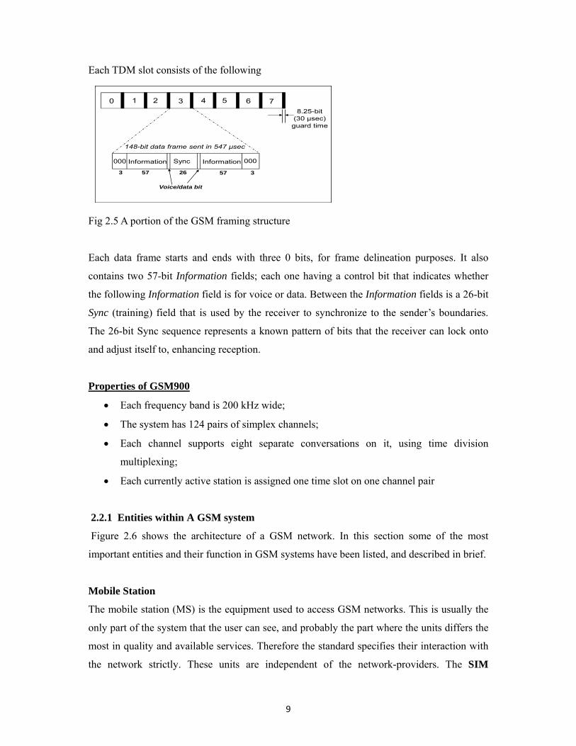
Each TDM slot consists of the following

0 1 2 3 4 5 6 7

000 Information Sync Information 000

Voice/data bit

35757 263

148-bit data frame sent in 547 μsec

8.25-bit(30 μsec)guard time

Fig 2.5 A portion of the GSM framing structure

Each data frame starts and ends with three 0 bits, for frame delineation purposes. It also

contains two 57-bit Information fields; each one having a control bit that indicates whether

the following Information field is for voice or data. Between the Information fields is a 26-bit

Sync (training) field that is used by the receiver to synchronize to the sender’s boundaries.

The 26-bit Sync sequence represents a known pattern of bits that the receiver can lock onto

and adjust itself to, enhancing reception.

Properties of GSM900

• Each frequency band is 200 kHz wide;

• The system has 124 pairs of simplex channels;

• Each channel supports eight separate conversations on it, using time division

multiplexing;

• Each currently active station is assigned one time slot on one channel pair

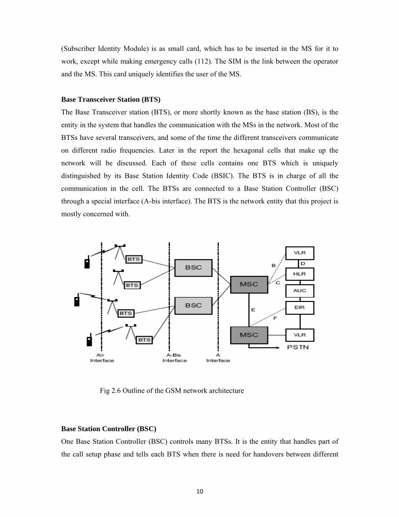
2.2.1 Entities within A GSM system

Figure 2.6 shows the architecture of a GSM network. In this section some of the most

important entities and their function in GSM systems have been listed, and described in brief.

Mobile Station

The mobile station (MS) is the equipment used to access GSM networks. This is usually the

only part of the system that the user can see, and probably the part where the units differs the

most in quality and available services. Therefore the standard specifies their interaction with

the network strictly. These units are independent of the network-providers. The SIM

   

  10

(Subscriber Identity Module) is as small card, which has to be inserted in the MS for it to

work, except while making emergency calls (112). The SIM is the link between the operator

and the MS. This card uniquely identifies the user of the MS.

Base Transceiver Station (BTS)

The Base Transceiver station (BTS), or more shortly known as the base station (BS), is the

entity in the system that handles the communication with the MSs in the network. Most of the

BTSs have several transceivers, and some of the time the different transceivers communicate

on different radio frequencies. Later in the report the hexagonal cells that make up the

network will be discussed. Each of these cells contains one BTS which is uniquely

distinguished by its Base Station Identity Code (BSIC). The BTS is in charge of all the

communication in the cell. The BTSs are connected to a Base Station Controller (BSC)

through a special interface (A-bis interface). The BTS is the network entity that this project is

mostly concerned with.

Fig 2.6 Outline of the GSM network architecture

Base Station Controller (BSC)

One Base Station Controller (BSC) controls many BTSs. It is the entity that handles part of

the call setup phase and tells each BTS when there is need for handovers between different

   

  11

cells. A BSC together with all the BTSs that it controls are often referred to as the Base

station Sub System (BSS).

Mobile Switching Center (MSC)

The Mobile Switching Center (MSC) is a switch connected to one or several BSCs. Its main

function is to switch speech and data connections between BSCs, other MSCs and mobile and

non-mobile networks. It is also connected to many different registers that are used to verify

each MS and call in the network.

Visitor Location Register (VLR)

It is integrated with the MSC to reduce the signaling link load between the two nodes. It is a

database containing information about all mobile subscribers currently located in the service

area of one MSC. Each MSC therefore has its own unique VLR. The VLR is responsible for

keeping track of a mobile’s position to the nearest location area.

Home Location Register (HLR)

It is a database in GSM which stores permanent subscriber’s data. It can be integrated in a

MSC/VLR node or implemented in a stand-alone node. When a subscriber registers in a new

MSC/VLR, the HLR function is to forward the subscriber information to that particular

MSC/VLR. Each time a subscriber changes MSC/VLR service area, it informs the HLR of its

new ‘address’ so that he/she can be reached when there is a call for him.

Authentication Center (AuC)

This is a database which prevents operators from fraud. It provides HLR with authentication

parameters and ciphering keys. It is implemented on an external computer, connected to the

HLR. The switch is also in charge of authenticating the mobile.

Equipment Identity Register (EIR)

It is a database that contains mobile equipment identity information, and includes list of

stolen, unauthorized or defective MSs. It checks whether the MS is stolen, and if so, prevents

any calls being made to or from it.

   

  12

2.2.2 The Radio Interface

The multiple access scheme used in GSM is a combination of FDMA and TDMA. This

means that the available bandwidth is split up in a larger number of frequency bands, and on

top of that each band is then divided in time to increase the amount of access channels. Going

back to the examples in Figure 2.1 and 2.2 (FDMA & TDMA), and combining these two, a

structure of the available bandwidth as in Figure 2.7 is obtained.

Fig 2.7 FDMA-TDMA

As previously mentioned, GSM has three dedicated base bands, the GSM900, GSM1800 and

the GSM1900. Each of these bands has a collective bandwidth of 50 MHz each. The 50 MHz

are divided in two 25 MHz bands, one used for uplink and the other for downlink. The two 25

MHz bands are then divided into 125 carrier frequencies each separated by 200 kHz. i.e. there

are 125 frequency for uplink and 125 for downlink, each 200 kHz wide. All 125 frequencies

are allocated in pairs so that each uplink/downlink pair is separated with exactly 45 MHz. In

Figure 2.8 we can see the bandwidth locations and separation relative to each other. The

structure is the same for GSM900, GSM1800 and GSM1900.

Fig 2.8 Frequency band allocations

Each of these 200 kHz bands is divided into 8 full-rate channels by using TDMA. These full-

rate channels will either be given a specific usage or split up in even smaller channels. The

total bit rate for one band is 270.833 kbit/s, and each channel is 22.8 kbit/s. When making a

call in a GSM network the MS will be assigned one out of all these channels. A channel in

GSM is one of these 200 kHz bands, discussed above, given a specific area of usage.

   

  13

2.2.3 Channel Structure

There are many different channels in GSM. The two most common channels used for

communication between a MS and a BTS are the TCH/F and TCH/H, which is Traffic

channel/Full-rate and half-rate. A full-rate channel is assigned one timeslot every 4.615 ms

and the half-rate channels gets as the name suggest half of a full-rate. This means that the

half-rate channels gets the entire available spectrum at their use, for a timeslot once every

9.23 ms. There is also a channel called TCH/8 which is an eighth of the full-rate channel.

These kinds of channels are mainly used as control channels. Below are some of the most

commonly used channels in GSM networks.

Traffic channels

A traffic channel (TCH) is used to carry speech and data traffic. Traffic channels are defined

using a 26-frame multiframe, or group of 26 TDMA frames. The length of a 26-frame

multiframe is 120 ms, which is how the length of a burst period is defined (120 ms divided by

26 frames divided by 8 burst periods per frame). Out of the 26 frames, 24 are used for traffic,

1 is used for the Slow Associated Control Channel (SACCH) and 1 is currently unused.

TCHs for the uplink and downlink are separated in time by 3 burst periods, so that the mobile

station does not have to transmit and receive simultaneously, thus simplifying the electronics.

In addition to these full-rate TCHs, there are also half-rate TCHs defined. Half-rate TCHs

effectively doubles the capacity of a system once half-rate speech coders are specified (i.e.,

speech coding at around 7 kbps, instead of 13 kbps). Eighth-rate TCHs are also specified, and

are used for signaling.

Control channels

There are many different control channels within the GSM specification that are assigned

different areas of usage. Common channels can be accessed both by idle mode and dedicated

mode mobiles. The common channels are used by idle mode mobiles to exchange the

signaling information required to change to dedicated mode. Mobiles already in dedicated

mode monitor the surrounding base stations for handover and other information. The

common channels are defined within a 51-frame multiframe, so that dedicated mobiles using

the 26-frame multiframe TCH structure can still monitor control channels. The common

channels include:

   

  14

Broadcast Control Channel (BCCH)

Continually broadcasts, on the downlink, information including base station identity,

frequency allocations, and frequency-hopping sequences.

Frequency Correction Channel (FCCH)

Used to synchronize the mobile to the time slot structure of a cell by defining the boundaries

of burst periods, and the time slot numbering. Every cell in a GSM network broadcasts

exactly one FCCH and one SCH, which are by definition on time slot number 0 (within a

TDMA frame).

Random Access Channel (RACH)

Slotted Aloha channel used by the mobile to request access to the network.

Paging Channel (PCH)

Used to alert the mobile station of an incoming call.

Access Grant Channel (AGCH)

Used to allocate an SDCCH (Stand Alone Dedicated Control Channel) to a mobile for

signaling (in order to obtain a dedicated channel), following a request on the RACH.

Synchronization Channel (SCH)

This channel supplies the time synchronization that all the MS’s needs to be able to

distinguish which time slot is up, and when to transmit. This channel periodically transmits a

distinguishable code that each MS synchronizes with. All the MS’s within the cells get the

same sense of time as the serving BS, but that “local” time will be different for all cells

within the net. Since all the BSs are asynchronous, it will allow the MSs to hear short periods

of control information from different BSs between the transmissions from the operating

BS. With this knowledge the mobile station can prepare for a handover if it would be

necessary.

   

  15

CHAPTER THREE

FREQUENCY PLANNING 3.1 Radio Network Planning

The objective of network planning and design is to provide wireless telephony services in a

serving area in the most cost-effective manner. In the case of existing system, the objective is

to expand and augment its facilities so as to add new features and capabilities or increase its

capacity in case the system has reached its coverage limit. The design usually involves

determining the number of base stations and their locations that would provide the necessary

coverage in the serving area, meet the desired grade of service, and satisfy the required traffic

growth so that the total startup cost is minimized and the rate of return maximized. The

network planning process and design criteria vary from region to region depending upon the

dominating factor, which could be capacity or coverage. The design process itself is not the

only process in the whole network design, and has to work in close coordination with the

planning processes of the core and especially the transmission network. A simplified process

just for radio network planning is shown in Figure 3.1.

The process of radio network planning starts with collection of the input parameters such as

the network requirements of capacity, coverage and quality. These inputs are then used to

make the theoretical coverage and capacity plans. Definition of coverage would include

defining the coverage areas, service probability and related signal strength. Definition of

capacity would include the subscriber and traffic profile in the region and whole area,

availability of the frequency bands, frequency planning methods, and other information such

as guard band and frequency band division. The radio planner also needs information on the

radio access system and the antenna system performance associated with it. The pre-planning

process results in theoretical coverage and capacity plans. There are coverage-driven areas

and capacity-driven areas in a given network region. The average cell capacity requirement

per service area is estimated for each phase of network design, to identify the cut-over phase

where network design will change from a coverage-driven to a capacity-driven process.

While the objective of coverage planning in the coverage-driven areas is to find the minimum

number of sites for producing the required coverage, radio planners often have to experiment

with both coverage and capacity, as the capacity requirements may have to increase the

number of sites, resulting in a more effective frequency usage and minimal interference.

   

  16

Candidate sites are then searched for, and one of these is selected based on the inputs from

the transmission planning and installation engineers.

After site selection, assignment of the frequency channel for each cell is done in a manner

that causes minimal interference and maintains the desired quality. Frequency allocation is

based on the cell-to-cell channel to interference (C/I) ratio. The frequency plans need to be

fine-tuned based on drive test results and network management statistics. Parameter plans are

drawn up for each of the cell sites. There is a parameter set for each cell that is used for

network launch and expansion. This set may include cell service area definitions, channel

configurations, handover and power control, adjacency definitions, and network-specific

parameters.

The final radio plan consists of the coverage plans, capacity estimations, interference plans,

power budget calculations, parameter set plans, frequency plans, etc.

Fig 3.1 Radio network planning process

3.1.1 The Automatic Frequency Planning (AFP) Problem

The frequency planning is the last step in the layout of a GSM network. Prior to tackling this

problem, the network designer has to address some other issues: where to install the BTSs or

how to set configuration parameters of the antennas (tilt, azimuth, etc.), among others. Once

the sites for the BTSs are selected and the sector layout is decided, the number of TRXs to be

installed per sector has to be fixed. This number depends on the traffic demand which the

corresponding sector has to support. The result of this process is a quantity of TRXs per cell.

A channel has to be allocated to every TRX and this is the main goal of the AFP. Essentially,

three kinds of allocation exist: Fixed Channel Allocation (FCA), Dynamic Channel

Allocation (DCA), and Hybrid Channel Allocation, discussed later in this report. In FCA, the

channels are permanently allocated to each TRX, while in DCA the channels are allocated

dynamically upon request. Hybrid Channel Allocation schemes (HCA) combine FCA and

DCA.

   

  17

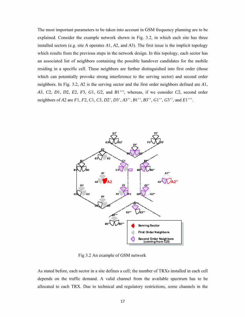
The most important parameters to be taken into account in GSM frequency planning are to be

explained. Consider the example network shown in Fig. 3.2, in which each site has three

installed sectors (e.g. site A operates A1, A2, and A3). The first issue is the implicit topology

which results from the previous steps in the network design. In this topology, each sector has

an associated list of neighbors containing the possible handover candidates for the mobile

residing in a specific cell. These neighbors are further distinguished into first order (those

which can potentially provoke strong interference to the serving sector) and second order

neighbors. In Fig. 3.2, A2 is the serving sector and the first order neighbors defined are A1,

A3, C2, D1, D2, E2, F3, G1, G2, and B1’’’, whereas, if we consider C2, second order

neighbors of A2 are F1, F2, C1, C3, D2’, D3’, A3’’, B1’’, B3’’, G1’’, G3’’, and E1’’’.

Fig 3.2 An example of GSM network

As stated before, each sector in a site defines a cell; the number of TRXs installed in each cell

depends on the traffic demand. A valid channel from the available spectrum has to be

allocated to each TRX. Due to technical and regulatory restrictions, some channels in the

   

  18

spectrum may not be available in every cell. They are called locally blocked and they can be

specified for each cell. Each cell operates one Broadcast Control CHannel (BCCH), which

broadcasts cell organization information. The TRX allocating the BCCH can also carry user

data. When this channel does not meet the traffic demand, some additional TRXs have to be

installed to which new dedicated channels are assigned for traffic data. These are called

Traffic CHannels (TCHs). In GSM, significant interference may occur if the same or adjacent

channels are used in neighboring cells. Correspondingly, they are named co-channel and

adjacent channel interference. Many different constraints are defined to avoid strong

interference in the GSM network. These constraints are based on how close the channels

assigned to a pair of TRXs may be. These are called separation constraints, and they seek to

ensure the proper transmission and reception at each TRX and/or that the call handover

between cells is supported. Several sources of constraint separation exist: co-site separation,

when two or more TRXs are installed in the same site, or co-cell separation, when two TRXs

serve the same cell (i.e., they are installed in the same sector).

3.1.2 The Cellular Concept and Frequency Reuse

The radio access part of the wireless network is considered of essential importance as it is the

direct physical radio connection between the mobile equipment and the core part of the

network. In order to meet the requirements of the mobile services, the radio network must

offer sufficient coverage and capacity while maintaining the lowest possible deployment

costs. One main issue in cellular system design reduces to one of economics. Essentially there

is limited resource transmission spectrum that must be shared by several users. Unlike wired

communications which benefits from isolation provided by cables, wireless users within close

proximity of one another can cause significant interference to one another. To address this

issue, the concept of cellular communication was introduced, where a given geographic area

is divided into hexagonal cells.

Each cell is allocated a portion of the total frequency spectrum. As users move into a given

cell, they are then permitted to utilize the channel allocated to that cell. The virtue of the

cellular system is that different cells can use the same channel given that the cells are

separated by minimum distance according to the system propagation characteristics,

otherwise intercellular or co-channel interference occurs. The minimum distance necessary to

reduce co-channel interference is called the reuse distance. The reuse distance is defined as

the ratio of the distance, D, between cells that use the same channel without causing

   

  19

interference and the cell radius, R as shown in figure 3.3. R is the distance from the centre of

a cell to the outermost point of the cell in cases where the cells are not circular. Typically

spatial separation, either in distance, angle, or polarization of electromagnetic fields is

exploited for frequency reuse. In such a system capacity per unit area must be sufficient for

the density of users and their usage patterns.

D = Reuse distance

r = radius of cell

Figure 3.3 7-cell cluster

 

3.1.3 Selection of Frequency Reuse Patterns

Patterns

A pattern is a number of cells grouped together, with each cell allocated a certain number of

channels, which are pairs of two frequencies to enable full-duplex communication. This

entire group of cells is known as a cluster. One cluster serves a complete set of frequencies

ranging from the entire allocated spectrum of the operator. The cluster pattern is then

repeated throughout the required coverage area.

D

ij

r 

   

  20

Patterns come in fixed numbers, and are derived from the formula, N = i² + ij + j² (refer to

Appendix A). Typical cluster sizes include 3, 4, 7, 9, 12, 19 and 21; with the most common

configuration being a 7-cell cluster, shown in figure 3.3.

Factors of Consideration

Factors to consider when selecting patterns include co-channel interference, which is the

radio interference caused by placing two cells, which have been allocated the same channel,

too close together. This causes deterioration of signal quality and in severe cases, might cause

a call to be temporarily or permanently disconnected, affecting the Grade of Service of the

operator.

The minimum distance required between the centers of two cells, using the same channel to

maintain the desired signal quality, is known as the reuse distance (refer to Appendix A). The

longer the reuse distance, the smaller the co-channel interference level will be. However, a

reuse distance that is too long increases the number of cells per cluster, which in turn results

in lower reuse efficiency and less system capacity.

Thus, the frequency reuse pattern should be determined taking into consideration both the co-

channel interference level and the reuse efficiency.

Determining Cluster Size

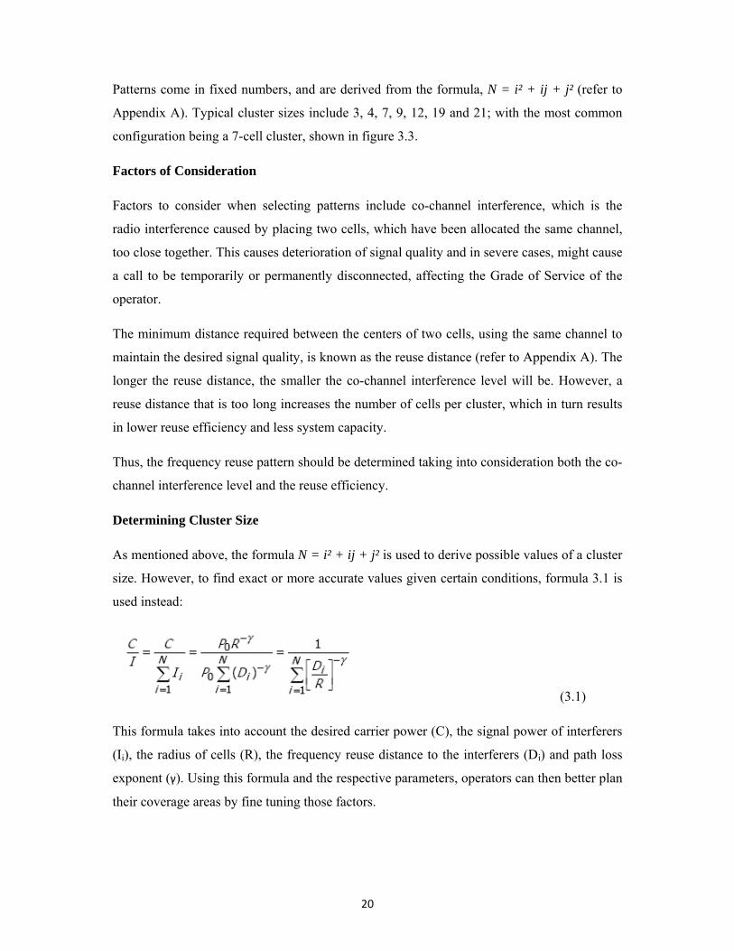
As mentioned above, the formula N = i² + ij + j² is used to derive possible values of a cluster

size. However, to find exact or more accurate values given certain conditions, formula 3.1 is

used instead:

(3.1)

This formula takes into account the desired carrier power (C), the signal power of interferers

(Ii), the radius of cells (R), the frequency reuse distance to the interferers (Di) and path loss

exponent (γ). Using this formula and the respective parameters, operators can then better plan

their coverage areas by fine tuning those factors.

   

  21

Implementation

In the course of preliminary planning, an operator would have thoroughly researched upon

and determined appropriate operational parameters such as the coverage radius of each cell,

placement of cells, and most importantly, the selection of the frequency reuse pattern derived

from the research and formula 3.1.

After being allocated a spectrum of frequencies from the respective regulator, the operator

will have to implement the plan by first determining the number of channels it can provide.

Then, the operator distributes the channels evenly among the cell cluster. The total number of

cells required for the desired coverage area is then calculated and the chosen cluster pattern is

repeated throughout the coverage area.

Testing will then be done to ensure the levels of co-channel interference and external

interference remain negligible, and following which the network will be fully functional for

commercial use.

Application

Due to the prevalence of frequency reuse, there is rarely a need to create an environment to

simulate application. The main problem that frequency reuse eliminates is the limitation of

allocated spectrum width to accommodate a higher number of mobile subscribers. Once

operators have chosen to implement frequency reuse, there will be an essential need to

strategically plan the distribution of cells and channels, and hence, decisively select a

frequency reuse pattern.

3.2 The Mobile Environment and Interference

Radio or wireless path normally described in wireless systems corresponds to the radio link

between a mobile user station and the base station with which it communicates. It is the base

station that is, in turn, connected to the wired network over which communication signals will

travel. Modern wireless systems are usually divided into geographically distinct areas called

cells, each controlled by a base station.

The focus here is on one cell and the propagation conditions encountered by signals

traversing the wireless link between the base station and mobile terminal. The link is made up

of two-way path: a forward path, downlink, from base station to mobile terminal; a backward

path, uplink, from mobile terminal to base station. The electromagnetic signals generated at

   

  22

either end will often encounter obstacles during the transmission, causing reflection,

diffraction, and scattering of the waves. The resultant electromagnetic energy reaching an

intended receiver will thus vary randomly. As a terminal moves, changing the conditions of

reception at either end, signal amplitudes will fluctuate randomly, resulting in fading of the

signal. The rate of fading is related to the relative speed of the mobile with respect to the base

station, as well as the frequency (or wavelength) of the signal being transmitted.

The important variables that define the mobile environment for a particular area include:

a) Physical terrain (Mountainous or hilly or flat or water).

b) Number, height, arrangement, and nature (construction materials) of man-made

structures.

c) Foliage and vegetation characteristics.

d) Normal and abnormal weather conditions.

e) Man-made radio noise.

Link budget defines the quality of the radio link, measured in terms of decibels (dB) or dBm,

where the ‘m’ stands for milliwatts, of signal power. A simplified link budget is given in

equation 3.2.

rtbmtPS GGLLLFLG −−++++= (3.2)

Gs = system gain in decibels

Lp = free space path loss in dB

F = fade margin in dB

Lt = transmission line loss from waveguide or coaxials used to connect radio to antenna, in

dB

Lm = miscellaneous losses such as minor antenna misalignment, waveguide corrosion, and

increase in receiver noise figure due to ageing, in dB

   

  23

Lb = branching loss due to filter and circulator used to combine or split transmitter and

receiver signals in a single antenna.

Gt = gain of transmitting antenna

Gr = gain of receiving antenna.

3.2.1 Adjacent Channel Interference

The carrier to adjacent ratio is defined as the signal strength ratio between a serving carrier

and an adjacent carrier. Interference from adjacent channels may sometimes be serious in a

mobile radio environment. Consider for example figure 3.4 where two mobile stations, MS1

and MS2, are transmitting on two adjacent channels. If the distance r2 from mobile MS2 to

the BTS is, say 10 times or more greater than the distance r1 of MS1, the signal received at

the BTS from MS1 may be over 40 dB higher than the signal from MS2. Furthermore,

because of fading, it is possible that the signal from MS2 is in a deep fade while the other

signal is above its local mean. Consequently, it becomes necessary to assign the channels in

such a way that there are no adjacent channels in the same set. This can be done in the

following way. Suppose that there are only 21 voice channels in the available spectrum block.

The channels may then be divided into seven sets, each with three channels, using channels

1,8, and 15 in set 1; channels 2, 9, and 16 in set 2; channels 3, 10, and 17 in set 3; and so on.

Figure 3.4 Adjacent channel interference

   

  24

However, in the previous assignment, even though no cell contains an adjacent channel, any

two adjacent cells will always have some adjacent channels between them. For example, cell

1 has channels 1, 8, and 15, and cell 2 has channels 2, 9, and 16. If base stations are located at

the center of a cell and use omnidirectional antennas, adjacent channels will cause

interference in any cell. This can be avoided by use of sectorised cells. By simply allocating

the channels to the directional antennas in a specific way, the interference due to adjacent

channels can be reduced to a satisfactory level. It is also possible to control adjacent channel

interference completely through filtering of both the transmitter and receiver to ensure that no

energy is transmitted outside the desired band and that the receiver filters out any unwanted

out-of-band energy.

3.2.2 Co-channel Interference

It is well known that one of the major limitations in cellular wireless telephone networks is

the so-called co-channel interference. In the case of TDMA networks, such as GSM/GPRS,

the co-channel interference is mainly caused by the spectrum allocated for the system being

reused multiple times (“frequency reuse”). The problem may be more or less severe,

depending on the reuse factor, but in all cases, a signal received by a handset will contain not

only the desired forward channel from the current cell, but also signals originating in more

distant cells.

The carrier-to-channel interference ratio (C/I) is the fundamental parameter in calculations of

reuse factors. It determines the degree of reuse and spectrum efficiency that can be achieved

in a cellular architecture. It is not possible to reuse frequencies in adjacent cells as the

boundary conditions would be characterized by nearly balanced signal levels from competing

transmitters and no communication would be possible. It is the isometric contour of co-

channel interference, not of signal level, that defines the cell boundary. The amount of

separation between cells using the same frequency is driven by;

a) The C/I ratio that is required to achieve the desired transmission quality.

b) The fade margin that is necessary to take care of statistical fluctuations in desired

signal level induced by the mobile environment. The fade margin is determined by

the maximum fades likely to be experienced, given the particular set of

countermeasures e.g. antenna diversity, being employed by the receiver.

   

  25

3.2.3 Methods of Reducing Co-channel Interference

Cellular systems are limited by interference. In these systems, multiple co-channel

interference, though controlled, is a normal situation, and is the main factor to determine the

service area/capacity. The goal is to allow the higher interference level in order to reuse the

available frequencies within the smallest area. As quality of service depends on the

carrier/interference ratio (CIR) more than on the signal/noise ratio, there is a certain trade-off

between quality and capacity that can be tolerated by the system.

Mobile markets have the larger growing rates among telecommunication markets. For this

growing rate to continue, higher levels of capacity and quality are needed. This means that all

possible techniques must be used to improve such features in order to reach a progressive

enhancement of the radio and network performance. Current implementation of GSM has

some powerful mechanisms intended to reduce the effect of interference such as slow

frequency hopping (SFH), discontinuous transmission (DTX) and power control, among

others.

1. Slow Frequency Hopping(SFH)

Slow Frequency Hopping (SFH) involves changing the frequency of the channel in every

transmitted burst (217 hops per second) providing frequency diversity and interference

averaging. This allows randomising the risk of interference and improving the behaviour of

the channel (for the selective fadings). The frequency hopping can be classified in two

categories: base band hopping and synthesiser hopping. Synthesiser hopping uses only one

transmitter for all burst belonging to a specific connection and the base band hopping uses as

many transmitter frequencies in the hopping sequence as possible. Synthesiser hopping is

more efficient and flexible. If we consider the way of changing the frequency, the hopping

can be also cyclic or random.

There are many factors affecting the performance of the SFH which include;

• Number of hopping frequencies: The higher the number of hopping frequencies the

better the system performance as it improves frequency diversity. However, using

more than 8 hopping frequencies does not provide a significant improvement due to

the GSM interleaving period of 8 bursts.

   

  26

• Hopping frequencies separation: The larger the frequency separation between the

hopping frequencies, the better the system performance as the effects of propagation

become more uncorrelated.

• System load: It has a direct influence in the SFH performance. Low system load

means lower interference probability in each hopping frequency and therefore, more

benefits from SFH.

• Frequency plan: When SFH is activated, a conventional frequency reuse scheme

based on a worst case interference situation is spectrally inefficient. Results show the

limitations of different frequency plans introducing this additional parameter in the

analysis, proposing a reuse scheme. Tighter reuse schemes can be achieved with the

use of the SFH providing more capacity.

2. Discontinuous Transmission(DTX)

DTX is used to suspend the radio transmission during the silence periods. This exploits the

observation that only 40-50% during a conversation does the speaker actually talk. DTX

helps also to reduce interference between different cells and to increase system capacity. It

prolongs battery charge life. The DTX function is performed by means of:

• Voice Activity Detection (VAD), which has to determine whether the sound

represents speech or noise, even if the background noise is very important. If the voice signal

is considered as noise, the transmitter is turned off producing then, an unpleasant effect called

clipping.

• Comfort noise. A side-effect of the DTX function is that when the signal is

considered as noise, the transmitter is turned off and therefore, a total silence is heard at the

receiver. This can be very annoying to the receiving user since it appears as a dead

connection. In order to overcome this problem, the receiver creates a minimum of

background noise called comfort noise. Comfort noise eliminates the impression that the

connection is dead.

3. Power Control

The power that is transmitted both from the mobile equipment and from the base station has a

far-reaching effect on efficient usage of the spectrum. Power control is an essential feature in

   

  27

mobile networks, in both the uplink and downlink directions. When a mobile transmits high

power, there is enough fade margin in the critical uplink direction, but it can cause

interference to other subscriber connections. The power should be kept to a level that the

signal is received by the base station antenna above the required threshold without causing

interference to other mobiles. Mobile stations thus have a feature such that their power of

transmission can be controlled. This feature is generally controlled by the BSS. This control

is based on an algorithm that computes the power received by the base station and, based on

its assessment, it increases or decreases the power transmitted by the mobile station.

3.2.4 Path loss

Path loss (or path attenuation) is the reduction in power density (attenuation) of an

electromagnetic wave as it propagates through space. Path loss is a major component in the

analysis and design of the link budget of a telecommunication system. This term is

commonly used in wireless communications and signal propagation. Path loss may be due to

many effects, such as free-space loss, refraction, diffraction, reflection, aperture-medium

coupling loss, and absorption. Path loss is also influenced by terrain contours, environment

(urban or rural, vegetation and foliage), propagation medium (dry or moist air), the distance

between the transmitter and the receiver, and the height and location of antennas.

The strength of the transmitted signal decreases in power relative to the distance between the

transmitter and the receiver. The standard rule for the path loss is that the signal strength

decreases as a factor R-γ, where R is the distance and γ is an environment dependent variable,

called path loss exponent. The value of γ varies between around 2-6, and for normal urban

environments the number is relatively close to 4. Lower values can appear in canyon-like

environments, for example at actual canyons or streets with tall buildings around.

Causes of Path Loss

Path loss normally includes propagation losses caused by the natural expansion of the radio

wave front in free space (which usually takes the shape of an ever-increasing sphere),

absorption losses (sometimes called penetration losses), when the signal passes through

media not transparent to electromagnetic waves, diffraction losses when part of the radio

wave front is obstructed by an opaque obstacle, and losses caused by other phenomena.

   

  28

The signal radiated by a transmitter may also travel along many and different paths to a

receiver simultaneously; this effect is called multipath. Multipath can either increase or

decrease received signal strength, depending on whether the individual multipath wavefronts

interfere constructively or destructively. The total power of interfering waves in a Rayleigh

fading scenario vary quickly as a function of space (which is known as small scale fading),

resulting in fast fades which are very sensitive to receiver position.

Path Loss exponent

In the study of wireless communications, path loss can be represented by the path loss

exponent, whose value is normally in the range of 2 to 4 (where 2 is for propagation in free

space, 4 is for relatively lossy environments and for the case of full specular reflection from

the earth surface, the so-called flat-earth model). In some environments, such as buildings,

stadiums and other indoor environments, the path loss exponent can reach values in the range

of 4 to 6. On the other hand, a tunnel may act as a waveguide, resulting in a path loss

exponent less than 2.

Path loss is usually expressed in dB. In its simplest form, the path loss can be calculated

using the formula

CdL += 10log10γ (3.1)

where L is the path loss in decibels, γ is the path loss exponent, d is the distance between the

transmitter and the receiver, usually measured in meters, and C is a constant which accounts

for system losses.

3.3 Channel Assignment Strategies

Channel Allocation

The capacity of a cellular system can be described in terms of the number of available

channels, or the number of users the system can support. The total number of channels made

available to a system depends on the allocated spectrum and bandwidth of each channel. The

available frequency spectrum is limited and the number of mobile users is increasing day by

day, hence the channels must be reused as much as possible to increase the system capacity.

Once the channels are allocated, cells may then allow users within the cell to communicate

   

  29

via the available channels. Channels in a wireless communication system typically consist of

timeslots, frequency bands and/or CDMA pseudo noise sequences, but in an abstract sense,

they can represent any generic transmission resource. There are three major categories for

assigning these channels to cells (or base stations). These are;

• Fixed Channel Allocation

• Dynamic Channel Allocation and

• Hybrid Channel Allocation.

3.3.1 Fixed Channel Allocation (FCA)

FCA systems allocate specific channels to specific cells. This allocation is static and cannot

be changed. For efficient operation, FCA systems typically allocate channels in a manner that

maximizes frequency reuse. Thus, in a FCA system, the distance between cells using the

same channel is the minimum reuse distance for that system. The problem with FCA systems

is quite simple and occurs whenever the offered traffic to a network of base stations is not

uniform. Consider a case in which two adjacent cells are allocated N channels each. There

clearly can be situations in which one cell has a need for N+k channels while the adjacent cell

only requires N-m channels (for positive integers k and m). In such a case, k users in the first

cell would be blocked from making calls while m channels in the second cell would go

unused. In this situation of non-uniform spatial offered traffic, the available channels are not

being used efficiently.

3.3.2 Dynamic Channel Allocation (DCA)

DCA attempts to alleviate the problem of FCA system when offered traffic is non-uniform. In

DCA systems, no relationship exists between channels and cells. Instead, channels are part of

a pool of resources. Whenever a channel is needed by a cell, the channel is allocated under

the constraint hat frequency reuse requirements can not be violated. There are two problems

that typically occur with DCA based systems.

• DCA methods typically have a degree of randomness associated with them and this

leads to the fact that frequency reuse is often not maximized unlike the case for FCA

   

  30

systems in which cells using the same channel are separated by the minimum reuse

distance.

• DCA methods often involve complex algorithms for deciding which available channel

is most efficient. These algorithms can be very computationally intensive and may

require large computing resources in order to be real-time.

The role of DCA is to allocate channels to cells or mobiles in such a way as to minimize;

a) The probability that the incoming calls are dropped

b) The probability that ongoing calls are dropped

c) The probability that the carrier-to-interference ratio (C/I) of any call falls below a

prespecified value.

The goal is to maximize the frequency reuse. In DCA there is no permanent allocation of

channels to cells. Rather, the entire set of available channels is accessible to all the cells, and

the channels are assigned on a call-by-call basis in a dynamic manner.

DCA schemes can be implemented as centralized or distributed.

Centralized DCA schemes

In this scheme, all requests for channel allocation are forwarded to a channel controller that

has access to the system wide channel usage information. The central controller then assigns

the channel by maintaining the required signal quality. The First Available (FA) is the

simplest method where the first available channel within the reuse distance encountered

during a channel search is assigned to the new call. Future blocking probability is a very

important factor for the channel selection in a new call.

Distributed DCA schemes

In this scheme the decision regarding the channel acquisition and release is taken by the

concerned BTS on the basis of the information from the surrounding cells. As the decision is

not based on the global status of the network, it can achieve only suboptimal allocation

compared to the centralized DCA and may cause forced termination of ongoing calls. This

scheme is based on co-channel distance, signal strength measurement and signal to noise

interference ratio. Centralized schemes can theoretically provide near optimal performance,

   

  31

but the amount of computation and communication among BTSs lead to excessive system

latencies and make them impractical. Therefore, distributed DCA schemes have been

proposed that involve scattering of channels across a network. A channel is selected for a new

call from its cell or interfering neighbouring cells.

3.3.3 Hybrid Channel Allocation

This includes all systems that hybrids of fixed and dynamic channel allocation systems.

Several methods fall within this category.

Channel Borrowing is one of the hybrid allocation schemes. Here, channels are assigned to

cells just as in fixed allocation schemes. If a cell needs a channel in excess of the channels

previously assigned to it, that cell may borrow a channel from one of its neighbouring cells

given that a channel is available and use of this channel won’t violate frequency reuse

requirements. Since every channel has a predetermined relationship with a specific cell,

channel borrowing is often categorized as a subclass of fixed allocation schemes. The major

problem with channel borrowing is that when a cell borrows a channel from a neighbouring

cell, other nearby cells are prohibited from using the borrowed channel because of co-channel

interference. This can lead to increased call blocking over time. To reduce this call blocking

penalty, algorithms are necessary to ensure that the channels are borrowed from the most

available neighbouring cells i.e. the neighbouring cells with the most unassigned channels.

Two extensions of the channel borrowing approach are Borrowing with Channel Ordering

(BCO) and Borrowing with Directional Channel Locking (BDCL).

• BCO systems have two distinctive characteristics;

1. The ratio of fixed to dynamic channels varies with traffic load.

2. Primary channels are ordered such that the first primary channel of a cell has the

highest priority of being applied to a call within the cell. The last primary channel is most

likely to be borrowed by neighbouring channels. Once a channel is borrowed, that channel is

locked in the co-channel cells within the reuse distance of the cell in question. From a

frequency reuse standpoint, in a BCO system, a channel may be borrowed only if it is free in

the neighbouring co-channel cells.

   

  32

• In BDCL, borrowed channels are only locked in nearby cells that are affected by the

borrowing. The benefit is that more channels are available in the presence of borrowing and

subsequent call blocking is reduced.

A natural extension to channel borrowing is to set aside a portion of the channels in a system

as dynamic channels with the remaining (primary) channels being fixed to specified cells. If a

cell requires an extra channel, instead of borrowing the channel from a neighbouring cell, the

channel is borrowed from the common ‘bank’ of dynamic channels.

   

  33

CHAPTER FOUR

PROPOSED FREQUENCY REUSE STRATEGY

4.1 The Frequency Reuse Pattern

A reuse pattern using clusters of 3 cells is proposed, where each of these 3 cells uses a

different subset of the available channels. Each cluster of cells uses the same channels in this

manner. Cells that use the same frequency are far enough apart that the interfering signals

received in any cell from co-channel cells are much weaker than the signals that originate

within that cell. For planning purposes, the cells are considered to be hexagonal, although in

practice their shapes are determined by radio coverage and they are irregular. For K-cell

frequency reuse, the distance between co-channel cells is KD 3= R where R is the cell

radius. In most systems, the interference is much stronger than the noise, and the SINR is

approximately equal to the carrier-to-interference ratio or C/I, which is used in the following

equations. The most significant interference comes from the six closest co-channel cells, so γ

⎟⎠⎞

⎜⎝⎛=

RD

IC

61 (4.1)

where γ is an empirically determined path loss exponent. For free space γ = 2. For suburban

and urban areas γ can be as high as 5 or 6, but is typically between 3 and 4. For the proposed

system model K=3 and γ is taken to be 3.3, thus D = 3R, and the C/I is calculated to be

3.3361

⎟⎠⎞

⎜⎝⎛=

RR

IC = 6.257 (power ratio) or (4.2)

10 log106.257 = 7.963 dB. (4.3)

This is far below the recommended GSM C/I of 9 dB and will cause significant co-channel

interference. In the proposed system therefore the cells are further divided into three sectors

each as shown in figure 4.3. For example cell A3 is divided into sectors A31, A32 and A33.

Each of these sectors is assigned a unique frequency to minimize adjacent channel and co-

channel interferences. Directional antennas are used so that each cell sector sees interference

primarily from two of the six closest co-channel cells. In this case C/I is given by

γ

⎟⎠⎞

⎜⎝⎛=

RD

IC

21 . (4.4)

   

  34

This is a 4.8 dB improvement over the C/I of a system with non-sectorised cells. For a three

sector system with K=3 and γ=3.3, C/I is calculated to be

3.3321

⎟⎠⎞

⎜⎝⎛=

RR

IC = 18.77 (power ratio) or 12.73 dB, (4.5)

which is above the threshold of 9 dB that is required for GSM systems. By the central limit

theorem, as the number of interferers becomes large, the total interference will tend towards a

Gaussian distribution and will resemble AWGN. Using this, capacity is approximated as

[ ]SINRBC T += 1log2 (4.6)

where SINR ≈ C/I. A single frequency band can be reused throughout the area, and the

capacity per unit area becomes

[ ]2

2 1logRK

SINRBAC T

Π+

= (4.7)

where A = area. In practice, the same modulation and coding techniques are used throughout

a communication system, and each technique has a minimum SINR threshold that must be

exceeded to achieve satisfactory performance. To maximize capacity, the minimum K that

will provide acceptable SINR is used. From equation 4.7 it is seen that decreasing R will also

increase capacity per unit area, but this approach is very expensive because it requires more

base stations. Systems that use small cells can also experience higher interference levels

because the path loss exponent γ in carrier to interference equations tends to be distance-

dependent. As the cell radius is decreased, the path loss exponent γ approaches 2 because

unobstructed line-of-sight propagation is more likely in smaller cells. From both equations, it

can be seen that if γ decreases, C/I (and SINR) decrease if the cellular reuse factor K, and

hence the D/R ratio, are fixed. Thus, if the cell radius is decreased too much, K must be

increased to maintain acceptable SINR, and this reduces the capacity per unit area.

Approaches have been proposed that use adaptive antennas to reduce interference and allow a

smaller K and increase capacity.

4.2 System Model

Consider a geographical area divided into 6 × 6 hexagonal cells, each cell having a radius of

R as shown in figure 4.1. The distribution of channels among the cells in the system, based on

resource planning model with cluster size 3 is assumed. The cluster size 3 means all channels

   

  35

in the allocated spectrum are assigned in three adjacent cells, if a channel is being used in any

cell, then none of the remaining two adjacent neighbouring cells can use this channel. The

considered minimum reuse distance (Dmin) is 3R, therefore the number of cells in interfering

neighbours is 6. If a channel r is being used in a cell then none of its interference

neighbouring cells can use r. When a MS wants to set up a call it sends request message to its

immediate BTS, if there exist some free primary channels in the requesting cell, then the BTS

will pick one in such a way that there will be no co-channel interference and channel

utilization is maximized.

If a channel is allocated for supporting the communication session between the MS and BTS,

then two cells can use the same channel only when the physical distance is not less than the

threshold distance Dmin, otherwise their communication session interfere with each other i.e.

co-channel interference.

Some of the channel selection schemes use resource planning model to get better channel

reuse for which the prior knowledge of channel status is required. The rules for using

resource planning model are as follows;

a) The set of cells is divided into a number of disjoint subsets such that any two cells in

the same subset are physically separated with at least a minimum reuse distance. The set of

channels are also divided into equivalent disjoint subsets.

b) The channels in the disjoint subsets are primary channels of cells in the subset and

secondary channels to another subset.

c) When all primary channels are exhausted, then a cell requests the secondary channels.

   

  36

Fig 4.1 The cellular system model

4.3 The proposed Algorithm

The cells are divided into 3 linear disjoint subsets i.e. A, B, C. Each of these 3 cells uses a

different subset of the available channels. Each cell has 6 neighbours. Consider a total of 18

channels available, hence each cell has 6 primary channels with the following channel

numbers;

Subset A: 1, 4, 7, 10, 13, 16

Subset B: 2, 5, 8, 11, 14, 17

Subset C: 3, 6, 9, 12, 15, 18

Channels 1, 2 and 3 are BCCHs and are used to broadcast the base station identity and

channel availability information. The subsets are disjointed to avoid adjacent channel

interference. The following assumptions are made;

• The terrain of the considered geographical area is flat such that channel fading is not

accounted for in this system.

• Neighbours of each cell in the system are defined. For example the neighbours of cell

A3 are defined as B1, C1, B3, C3, B5, and C5 as shown in figure 4.2.

   

  37

Figure 4.2 Defining cell neighbours

• All BTSs transmit at the same power and they are centrally located in the cell.

• Directional antennas are used in the sectorised cells where each cell has 3 sectors as

shown in figure 4.3, where each sector is assigned two channels hence two TRXs

installed.

Figure 4.3 sectorised system model

   

  38

A cell, say A3, needs a channel to support a call request. It first checks free primary channels,

if available it picks the least and marks it as used channel and supports that call immediately.

Otherwise A3 changes to search mode and sends request to all its interfering neighbours, Nx

(i.e. B1, C1, B3, C3, B5, and C5). When a cell in Nx receives a request from A3, it sends a

reply Px-Ux=Bx , where Px are the primary channels in that cell, Ux are the channels in use and

Bx are the unused channels which can be borrowed. When A3 receives reply messages from

Nx , it selects a channel randomly from the largest Bx or if two or more Bxs are equal, it

selects a channel from the first to arrive.

A3 takes confirmation of selected channel to the lender which marks this channel as an

interference channel; the channel cannot be used until it is returned by the borrower. The call

is blocked if no free available channel is left. This is depicted in the flow chart of figure 4.4.

   

  39

Figure 4.4 Flow chart of the channel allocation algorithm

   

  40

4.4 Explanation of the Algorithm

A channel allocation algorithm includes a channel acquisition and a channel selection

scheme. Most distributed DCA algorithms are based on non-resource planning model in

which a borrower needs to consult with every interfering neighbor in order to borrow a

channel. The proposed algorithm makes efficient reuse of channels. The purpose of this

scheme is to assign channels in such a way so that channel utilization is maximized at the

same time maintaining the voice quality.

Channel acquisition

The task of channel acquisition phase is to collect information of free available channels

from the interfering cells and ensure that two cells within the minimum reuse distance do not

share the same channel.

Channel selection

The channel selection phase is concerned with choosing a channel from the number of

available free channels in order to get better channel utilization in terms of channel reuse. The

acquisition phase of the distributed DCA algorithm consists of two approaches namely search

and update. In search approach, when a cell requires a channel, it searches from all its

interfering neighbours to find the currently free available channels from which it selects one

channel according to the underlying selection scheme. In the update approach, a cell

maintains information about free available channels. When a cell requires a channel, the

channel selection scheme is used to pick one available channel and confirms with its

interfering neighbouring cells whether it can use the selected channel or not. After that, when

a cell acquires or releases a channel at any time, it informs its interference neighbours so that

every cell in the system model always knows the available channels of its interference

neighbouring cells. Fast carrier returning should be used to increase channel utilization by

returning the borrowed channels as soon as possible. Consider a cluster size of 3 cells for

example. The number of channel sets is divided into 3 channel disjoint subsets. When a cell

needs to borrow a channel, it has to send request message to its 6 interfering neighbours.

   

  41

CHAPTER FIVE

SIMULATION RESULTS AND ANALYSIS

5.1 Description of Results

One of the most important characteristic of a cellular network is that a certain number of calls

will fail to establish an initial connection. Two measures can be stated for dealing with

unsuccessful call attempts: the never serviced new calls, and the delayed successful calls

(waiting for initial connection). The blocking probability is one of the most important

characteristics for the performance of a cellular network. When a new call arrival occurs and

the network cannot allocate a channel then we say that this call is blocked. The blocking

probability Pbl is calculated from the ratio

receivedcallscallsblockedPBL _

_= . Table 5.1 illustrates the blocking probabilities of the proposed DCA

scheme and FCA scheme which is currently being used by cellular network operators in the

country. These results were generated by simulating the program code dca.m in matlab. The

code is illustrated in Appendix C.

Table 5.1 Blocking probability simulation results Number of calls

Arriving in one cell

Number of calls

blocked in DCA

scheme (nb)

Number of calls

blocked in FCA

scheme (nb1)

Blocking

probability

In DCA (pbl)

Blocking

probability

In FCA (pbl1)

152 5 49 0.0329 0.3224

165 9 48 0.0545 0.2909

170 11 52 0.0647 0.3059

173 12 62 0.0694 0.3584

180 7 71 0.0389 0.3944

213 15 87 0.0704 0.4085

216 11 90 0.0509 0.4167

218 17 84 0.0780 0.3853

226 18 94 0.0796 0.4159

241 8 107 0.0331 0.4440

   

  42

The results in table 5.1 were used to plot the blocking probability curve of figure 5.1 for

comparison of the DCA and FCA frequency reuse schemes.

150 160 170 180 190 200 210 220 230 240 2500

0.05

0.1

0.15

0.2

0.25

0.3

0.35

0.4

0.45

prob

abili

ty o

f blo

ckin

g

number of calls arriving in one cell

Blocking probability vs call arrival

FCA scheme

DCA scheme

Figure 5.1 Blocking probability graph

   

  43

5.2 Analysis

The blocking probability of the proposed DCA algorithm is compared with that of FCA. The

DCA algorithm significantly reduces the call blocking rate, due to the channel borrowing and

reduction of the cluster size in resource planning model. In DCA scheme proposed the

number of cell congestion is smaller in contrast with FCA scheme, which means that the

network management is easiest in DCA.

The dropping probability is also an additional and very important characteristic of the cellular

network. When a call is in progress and the required quality conditions are not met then his

call is obligatory driven to termination. The dropping probability Pd is calculated from the

ratio

)__()__(__

numbercalldroppednumbercalltotalnumbercalldroppedPd −

= . This was taken care by

sectorization of the cells to improve the C/I ratio.

   

  44

CHAPTER SIX

CONCLUSIONS AND RECOMMENDATIONS

6.1 Conclusions of the results

In conclusion, this report has described the process of selecting frequency reuse patterns and

implementing them in mobile networks. It has discussed the required considerations in proper

planning, and the key factors in determining appropriate parameters to build a feasible and

robust network. The proposed channel allocation algorithm makes efficient reuse of channels

using resource planning model with reduction of the cluster size. The simulation results

shows that the blocking probability of the proposed DCA algorithm is significantly less than

that of FCA algorithm. The divergence between simulation results and real network behavior

is affected by the structure of the implementation algorithms and the corresponding research

of real network conditions like new call arrival schemes, user movement, etc. A deeper

research requires full customizable software with high level of adaptation in real network

specifications and behavior.

Future Development

As the selection of frequency reuse patterns is more of a concept and process rather than a

technology itself, the continued development into this area is dependent on the individual

standardization bodies or manufacturers who develop the standards. The results obtained are

promising but not conclusive. Comparison with other dynamic frequency allocation

algorithms is warranted. A solution similar to the one demonstrated here might one day be

considered by a cellular provider or implemented in an actual cellular network.

In future as these cellular networks become larger and more complex, extra functions could

be added to the proposed algorithm. These would include mobile environment effects and

different base station locations for a better generalization of the proposed algorithm and extra

functions for more reliable testing and frequency assignment. An algorithm to get a more

self-calibrating network of base stations could be developed to deploy the network that has

implemented the frequency planning algorithm proposed in this project. When the network is

up and running we could have all the base stations registering and saving the received SINRs

during a period of time. Using this data, a more sophisticated algorithm could be developed

that tunes the antennas in a similar manner to what is done by hand nowadays to make the

network close to self operating.

   

  45

CHAPTER SEVEN REFERENCES AND APPENDICES

References

[1] Mischa Schwartz, Mobile Wireless Communications, Cambridge University Press, 2005.

[2] J. Dunlop and D.G. Smith, Telecommunications Engineering, 3rd edition,

Chapman & Hall, University and Professional Division, 1994.

[3] Razavi B., RF Microelectronics, Prentice-Hall Inc., USA, 1998.

[4] Calhoun George, Digital Cellular Radio, Artech House, Inc, Norwood, USA, 1988.

[5] I.A. Glover and P.M. Grant, Digital Communications, Pearson Education Limited,

2nd edition, 2004.

[6] G.S.O. Odhiambo, FEE 522 Lecture Notes, Communication Networks and Information

Theory, University of Nairobi, 2009.

[7] P.M. Papazoglou, D.A. Karras, and R.C. Papademtriou, “A Dynamic Channel

Assignment Simulation System for Large Scale Cellular Telecommunications”, IEEE

Personal Communications, vol.5, No.1, 2004, pp. 10-31

[8] T.S. Rappaport, Wireless Communications: Principles and Practice, Prentice Hall, 2002.

[9] M. Zhang, and T.S. Yum, “Comparisons of Channel Assignment Strategies in Cellular

Mobile Telephone Systems”, IEEE Transactions on Vehicular Technology, vol.38, No.4,

pp211-215, 1989.

[10] M. Gupta, and A.K. Sachan, “Distributed Dynamic Channel Allocation Algorithm for

Cellular Mobile Network”, Journal of Theoretical and Applied Information Technology,

vol.1, No. 1, pp58-63, 2007.

   

  46

Appendices

Appendix A: Properties and Fundamentals of the Cellular Geometry

Let Radius of each cell = R

Let Distance between center of adjacent cells = d

Let Distance between centers of Co-channel Cells = D

Step 1: To find the relation between radius of cell (R) and distance d

Fig A1 Hexagonal geometry

From the figure A1,

CI = R/2; OI = d/2 and OC = R (A1)

By Pythagoras theorem

222 CIOIOC += (A2)

Applying equations (A1) into (A2),

   

  47

222

22⎟⎠⎞

⎜⎝⎛+⎟

⎠⎞

⎜⎝⎛=

RdR (A3)

Making d the subject of the formula,

Rd 3= (A4)

The figure A2 shows the most convenient set of coordinates for hexagonal geometry. The

positive halves of the two axes intersect at a 60° angle, and the unit distance along any of the

axis equals 3 R. The radius is defined as the distance from the center of a cell to any of its

vertices. Based on this, the center of each cell falls on a point specified by a pair of integer

coordinates.

Fig A2 Coordinates for hexagonal geometry

The first thing to note is that in this coordinate system the distance d12 between two points (U1,

V1) and (U2, V2) respectively is:

( ) ( ) ( )( ) °−−+−+−= 60cos2 12122

122

122

12 VVUUUUVVd (A5)

= ( ) ( ) ( )( )21*2 1212

212

212 VVUUUUVV −−+−+− (A6)

   

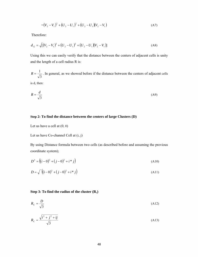
  48

= ( ) ( ) ( )( )12122

122

12 VVUUUUVV −−+−+− (A7)

Therefore:

( ) ( ) ( )( )][ 12122

122

1212 VVUUUUVVd −−+−+−= (A8)

Using this we can easily verify that the distance between the centers of adjacent cells is unity

and the length of a cell radius R is:

31

=R . In general, as we showed before if the distance between the centers of adjacent cells

is d, then:

3dR = (A9)

Step 2: To find the distance between the centers of large Clusters (D)

Let us have a cell at (0, 0)

Let us have Co-channel Cell at (i, j)

By using Distance formula between two cells (as described before and assuming the previous

coordinate system);

( ) ( )( )jijiD *00 222 +−+−= (A10)

( ) ( )( )jijiD *00 22 +−+−= (A11)

Step 3: To find the radius of the cluster (Rc)

3DRC = (A12)

3

22 ijjiRC

++= (A13)

   

  49

Step 4: To find the number of cells in a cluster (K) (i.e. cluster size)

K = Cluster Area/Cell Area (A14)

Single Cell Area = 6 * (Area of 1 triangle with equal edges R)

= ]2

*21[*6 dR (A15)

From (A4) we have that Rd 3= . Therefore:

Single Cell Area = 2*2

33]321*

21[*6 RRR = (A16)

Following similar reasoning the cluster area is:

Cluster Area = 2*2

33CR (A17)

Substituting equation (A16) and (A17) in (A14) we get,

2

2

RR

K C= (A18)

By substituting (A13) and (A4) in (A18) (assuming unit distance d=1) we get:

ijjiK ++= 22 (A19)

Step 5: To find Co-channel Reuse Ratio / Factor (Q)

Q = D/R (A20)

Substituting equation (A19), (A11) and (A4) in (A20) and also taking unit distance (i.e. d =1),

we get,

KQ 3= (A21)

   

  50

Appendix B: Dynamic Channel Allocation pseudocode.

Partition coverage area and assign channels to cells.

on {call arrival,} {

if ( primary channel available ) {

use smallest channel

}

else {

if (secondary channel available ) {

borrow largest from neighbour with maximum free channels

}

else {

block call

}

}

}

on { call termination } {

if ( secondary channel borrowed ) {

reassign and return

}

}

   

  51

Appendix C: Matlab simulation code for DCA and FCA schemes

%Channel allocation simulation code

sumnA3=0; %sum of calls arriving in cell A3 after a number of iterations

sumnb=0; % sum of calls blocked in DCA scheme in cell A3

sumnb1=0; % sum of blocked calls in FCA scheme for an equal number of calls

%arriving in cell A3

n1=1;

while n1 <= 25 % Defines number of iterations from 1 to 25

nA3=int16(rand(1)*15) %generates random number of calls in reference

%cell A3 i.e. nA3

%Define neighbours of cell of consideration (A3)and generate random number

%of calls in the neighbours of cell A3

nB1=int16(rand(1)*15);%number of calls in cell B1

nC1=int16(rand(1)*15);%number of calls in cell C1

nB3=int16(rand(1)*15);%number of calls in cell B3

nC3=int16(rand(1)*15);%number of calls in cell C3

nB5=int16(rand(1)*15);%number of calls in cell B5

nC5=int16(rand(1)*15);%number of calls in cell C5

sumnA3=sumnA3+nA3;

   

  52

%Channel Allocation through DCA scheme

%Declare condition to be met for supporting a call using primary channels

if nA3<=6

disp('Channel assignment in DCA scheme successful through primary channels');

else

if (nB1<6 || nC1<6 || nB3<6 || nC3<6 ||nB5<6 ||nC5<6 ) % condition of

%neighbour cells to lend free channels

n=nA3-6; % number of borrowed channels

disp ('Channel assignment in DCA scheme successful through borrowed channels');

else

nb = nA3-6 % If no free secondary channel available, call(s) is/are blocked

disp('calls blocked');

sumnb=sumnb+nb;

end

n1=n1+1;

end

%Fixed channel allocation (FCA) scheme

if nA3>6 % Condition for blocking calls in FCA scheme

disp('Corresponding number of calls blocked in FCA scheme is')

nb1=nA3-6 %number of blocked calls in one iteration

   

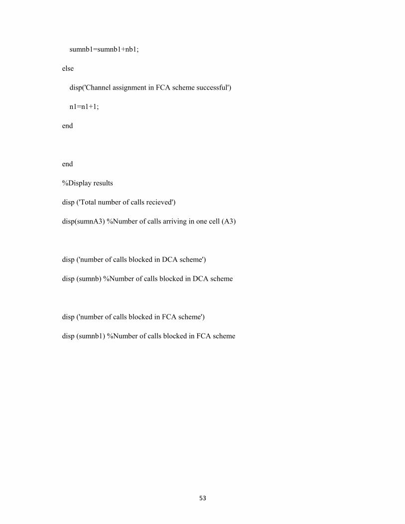
  53

sumnb1=sumnb1+nb1;

else

disp('Channel assignment in FCA scheme successful')

n1=n1+1;

end

end

%Display results

disp ('Total number of calls recieved')

disp(sumnA3) %Number of calls arriving in one cell (A3)

disp ('number of calls blocked in DCA scheme')

disp (sumnb) %Number of calls blocked in DCA scheme

disp ('number of calls blocked in FCA scheme')

disp (sumnb1) %Number of calls blocked in FCA scheme