Embed Size (px)
Citation preview
i
UNIVERSITY OF NAIROBI
DEPARTMENT OF ELECTRICAL AND INFORMATION ENGINEERING
DIGITAL CONTROL OF A LINE FOLLOWING ROBOT
PROJECT INDEX: PRJ 75
NAME: MUINDI DENNIS MUTHEKE D.
REG NO: F17/2454/2008
SUPERVISOR: PROF. J. M. MBUTHIA
EXAMINER: MR. MUSAU
Project report submitted in partial fulfillment of the requirement for the award of the Degree of: Bachelor of Science in Electrical and Electronic Engineering of the University of Nairobi.
Date of Submission:
24TH
APRIL 2015

ii
DECLARATION OF ORIGINALITY
I understand what plagiarism is and I am aware of the university policy in this regard.
1. I declare that this final year project report is my original work and has not been submitted elsewhere for examination, award of a degree or publication. Where other people’s work or my own work has been used, this has properly been acknowledged and referenced in accordance with the University of Nairobi’s requirements.
2. I have not sought or used the services of any professional agencies to produce this work.
3. I have not allowed, and shall not allow anyone to copy my work with the intention of passing it off as his/her own work.
4. I understand that any false claim in respect of this work shall result in disciplinary action, in accordance with University anti-plagiarism policy.
SIGNATURE: ………………………………………………………………………………………
DATE: ………………………………………………………………………………………………..
NAME OF STUDENT: Muindi Dennis Mutheke D REGISTRATION NUMBER: F17/2454/2008 COLLEGE: Architecture and Engineering
FACULTY/ SCHOOL/ INSTITUTE: Engineering DEPARTMENT: Electrical and Information Engineering COURSE NAME: Bachelor of Science in Electrical & Electronic Engineering TITLE OF WORK: Digital Control of a Line Following Robot
iii
CERTIFICATION
This project report has been submitted to the Department of Electrical & Information Engineering, University of Nairobi with my approval as supervisor.
Prof. J. Mwangi Mbuthia
SIGNATURE: ………………………………………………………………………………………
DATE: ……………………………………………………………………………………………….

iv
DEDICATION
I dedicate this project to the young robotics enthusiasts in Kenya. The robotic age is now upon us.

v
ACKNOWLEDGEMENTS
With a grateful heart, I would like to acknowledge all members of staff at the Department of Electrical and Information Engineering, University of Nairobi for their immense contributions in my academic endeavours. Thank you for everything you have done to me, day after day, year after year. I wish to express profound gratitude to my supervisor, Prof. J. M. Mbuthia for providing very vital assistance in acquisition of the Lego Mindstorms kit. I appreciate his timely review and thoughtful assessment of the project progress.
Fellow engineering students, you have been my steadfast companions in this scholarly journey.
I will forever treasure you for the unflinching support you gave me.
Special thanks to Daniele Benedettelli, Laurens Valk, Terry Griffin. You greatly nurtured my
interest in Lego Mindstorms robots.
To the Supreme Creator and Sustainer of the universe, your intelligent design concepts fill me
with wonder. I appreciate and value your grace, goodness and bountiful blessings in my life.
vi
Table of Contents
DECLARATION OF ORIGINALITY ............................................................................................................................. II
CERTIFICATION ..................................................................................................................................................... III
DEDICATION ......................................................................................................................................................... IV
ACKNOWLEDGEMENTS .......................................................................................................................................... V
TABLE OF CONTENTS ............................................................................................................................................. VI
LIST OF FIGURES .................................................................................................................................................. VIII
LIST OF TABLES ..................................................................................................................................................... IX
ABSTRACT .............................................................................................................................................................. X
CHAPTER 1 ............................................................................................................................................................. 1
1. INTRODUCTION .............................................................................................................................................. 1
1.1 DIGITAL CONTROL AND ROBOTICS: ........................................................................................................... 1
1.2 PROBLEM STATEMENT ................................................................................................................................ 1
1.3 OBJECTIVES ................................................................................................................................................... 1
1.3.1 OVERALL OBJECTIVE .......................................................................................................................................... 1
1.3.2 SPECIFIC OBJECTIVES ........................................................................................................................................................................ 1
PROJECT JUSTIFICATION ................................................................................................................................... 2
1.5 PROJECT SCOPE ............................................................................................................................................ 2
1.6 REPORT ORGANIZATION ............................................................................................................................. 2
CHAPTER 2 ............................................................................................................................................................. 4
2. LITERATURE REVIEW ......................................................................................................................................... 4
2.1 DIGITAL CONTROL SYSTEMS ............................................................................................................................ 4
2.1.1 INTRODUCTION .............................................................................................................................................. 4
2.1.2 WHY DIGITAL CONTROL? .................................................................................................................................. 5
2.1.3 TYPES OF CONTROLLERS............................................................................................................................... 6
2.2 LEGO MINDSTORMS EV3................................................................................................................................... 7
2.2.1 PARTS OF THE LINE FOLLOWING ROBOT .................................................................................................... 8
2.2.1.1. THE EV3 BRICK ........................................................................................................................................................................... 8 2.2.1.2. POWER SUPPLY .......................................................................................................................................... 8
2.2.1.3. CONNECTOR CABLES ................................................................................................................................. 9
2.2.1.4. BEAMS, CONNECTOR PEGS, AXLES AND BUSHES .................................................................................... 9
2.2.1.5. CROSS BLOCKS AND ANGLE ELEMENTS ................................................................................................. 10
2.2.1.6. WHEELS AND TIRES ................................................................................................................................. 10
2.2.1.7. COLOUR SENSOR ....................................................................................................................................... 10
2.2.1.8. SERVO MOTORS ................................................................................................................................... 11
2.2.1.8.1. MODELLING OF A DC SERVO MOTOR ................................................................................................... 12
2.2.1.8.2 DC SERVO MOTOR ENCODERS .................................................................................................................. 14
2.3 APPLICATIONS OF A LINE FOLLOWING ROBOT ........................................................................................... 15
vii
CHAPTER 3 ........................................................................................................................................................... 16
3. METHODOLOGY ............................................................................................................................................ 16
3.1 LEGO MINDSTORMS LINE FOLLOWER ROBOT DESIGN .......................................................................... 16
3.2. STUDY OF THE LEGO MINDSTORMS EV3 MOTOR .................................................................................. 17
3.2.1. MOTOR SPECIFICATIONS ............................................................................................................................ 17
3.2.2 EV3 SERVO MOTOR IMPLEMENTATION ON MATLAB:......................................................................... 17
3.2.3:S-DOMAIN EV3 SERVO MOTOR TRANSFER FUNCTION: .................................................................................. 18
3.2.4: Z-DOMAIN EV3 SERVO MOTOR TRANSFER FUNCTION: ................................................................................. 20
3.3 LINE FOLLOWING ROBOT ALGORITHMS ................................................................................................. 22
3.4: DIGITAL CONTROLLER DESIGN: ............................................................................................................... 23
3.4.1. PROPOSED CONTROLLER DESIGN: ............................................................................................................ 23
3.4.2: IMPLEMENTATION OF LINE FOLLOWING CONTROL ALGORITHM FOR THE LEGO MINDSTORMS EV3
HARDWARE: ............................................................................................................................................................ 24
CHAPTER 4 ........................................................................................................................................................... 26
4. RESULTS AND ANALYSIS .............................................................................................................................. 26
4.1: EV3 LARGE MOTOR CHARACTERISTICS .................................................................................................. 26
4.2: PID TUNING ................................................................................................................................................ 27
4.3: FREQUENCY RESPONSE ............................................................................................................................. 32
4.4.GENERAL ANALYSIS .................................................................................................................................... 33
CHAPTER 5 ........................................................................................................................................................... 35
5. CONCLUSION AND RECOMMENDATIONS.................................................................................................... 35
5..1 CONCLUSION .................................................................................................................................................... 35
5.2 RECOMMENDATIONS FOR IMPLEMENTATION ............................................................................................ 35
5.3 RECOMMENDATIONS FOR FURTHER WORK ................................................................................................ 35
6 REFERENCES ................................................................................................................................................... 36
APPENDIX A ....................................................................................................................................................... 38
A.1 MATLAB CODE FOR CHAPTER 3 ..................................................................................................................... 38
A.2 MATLAB CODE FOR CHAPTER 4 ..................................................................................................................... 40
APPENDIX B ......................................................................................................................................................... 42
viii
LIST OF FIGURES Fig 2-1: General configuration of a digital control system………………………………………………………………………4
Fig 2-2: Feedback loop with PD control …………………………………………………………………………….……..6
Fig 2-3: Feedback loop with PI control……………………………………………………………………………………………………7
Fig 2-4: Feedback loop with PID control……………………………………………………………………………………7
Fig 2-5: Front and back views of the EV3 Brick. The back is the 9V battery ……………………………..8
Fig 2-6: Connector cables …………………………………………………………………………………………………….9
Fig 2-7: A collection of Lego beams, axles, connector pegs and bushes…………………………………..9
Fig 2-8: A collection of Cross Blocks and Angle Elements……………………………………………………....10
Fig 2-9: Lego wheels ……………………………………………………………………………………………………………..10
Fig 2-10: EV3 Colour sensor and the measuring ranges in the ‘Colour’ and ‘Reflected Light
Intensity’ modes……………………………………………………………………………………………………………………..11
Fig 2-11: Large servo motor …………………………………………………………………………………………………………………12
Fig.2-12: Model of a servo motor………………………………………………………………………………………………………….12
Fig 2-12: Individual blocks and complete representation of DC servo motor ………………………………………14
Fig. 2-13: Motor encoder …………………………………………………………………………………………………………………….15
Fig. 3-1: Line Following Robot ………………………………………………………………………………………………………………16
Fig.3-2: Motor implementation on Simulink …………………………………………………………………………………………17
Fig.3-3: Step response of the s-domain servo motor transfer function …………………………………………………18
Fig. 3-4: Root Locus of the s-domain servo motor transfer function …………………………………………………….19
Fig. 3-5: Bode plot of the s-domain servo motor transfer function……………………………………………………….19
Fig 3-6: Step response of the z domain servo motor transfer function………………………………………………….20
Fig 3-7: Root Locus of the z-domain servo motor transfer function………………………………………………………21
Fig 3-8: Bode plot of the z-domain servo motor transfer function…………………………………………………………21
Fig 3-9: Basic line following approach……………………………………………………………………………………………………22
Fig 3-10: Simulink Line Tracking Program with PID Controller………………………………………………….24
Fig 4.1: Graph of rotation speed against applied voltage ……………………………………………………………………26
Fig 4.2: Step response: Kp =1 ………………………………………………………………………………………………….27
Fig 4.3: Step response: Kp =5 ………………………………………………………………………………………………….28
Fig 4.4: Step Response: Kp = 2.4 …………………………………………………………………………………………………………..29
Fig 4.5: Step response: Kp =2.4, Ki =0.01, Kd =0 ……………………………………………………………………………………30
Fig 4.6: Step Response: Kp =2.4, Ki = 0.01, Kd = 0.1 ………………………………………………………………………….31
Fig 4.7: Various frequency plots for the compensated system during tuning (Kp = 5) ………………………….32
Fig 4.8: Various frequency plots for the compensated system (Kp =2.4, Ki=0.01, Kd =0.1)………33
ix
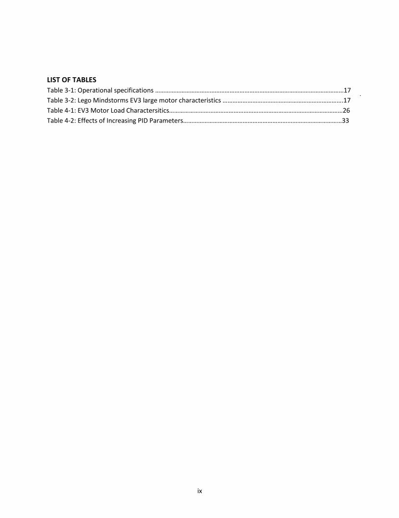
LIST OF TABLES
Table 3-1: Operational specifications ……………………………………………………………………………………………………17
Table 3-2: Lego Mindstorms EV3 large motor characteristics ……………………………………………………………….17
Table 4-1: EV3 Motor Load Charactersitics……………………………………………………………………………………………26
Table 4-2: Effects of Increasing PID Parameters……………………………………………………………………………………33
x
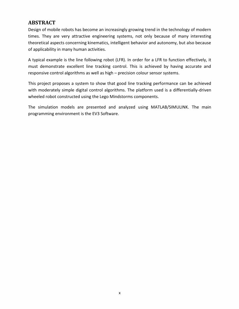
ABSTRACT
Design of mobile robots has become an increasingly growing trend in the technology of modern
times. They are very attractive engineering systems, not only because of many interesting
theoretical aspects concerning kinematics, intelligent behavior and autonomy, but also because
of applicability in many human activities.
A typical example is the line following robot (LFR). In order for a LFR to function effectively, it
must demonstrate excellent line tracking control. This is achieved by having accurate and
responsive control algorithms as well as high – precision colour sensor systems.
This project proposes a system to show that good line tracking performance can be achieved
with moderately simple digital control algorithms. The platform used is a differentially-driven
wheeled robot constructed using the Lego Mindstorms components.
The simulation models are presented and analyzed using MATLAB/SIMULINK. The main
programming environment is the EV3 Software.
1
CHAPTER 1
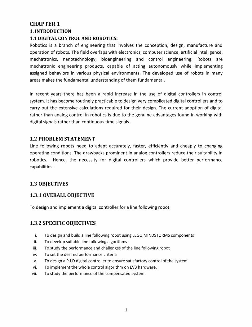
1. INTRODUCTION
1.1 DIGITAL CONTROL AND ROBOTICS:
Robotics is a branch of engineering that involves the conception, design, manufacture and
operation of robots. The field overlaps with electronics, computer science, artificial intelligence,
mechatronics, nanotechnology, bioengineering and control engineering. Robots are
mechatronic engineering products, capable of acting autonomously while implementing
assigned behaviors in various physical environments. The developed use of robots in many
areas makes the fundamental understanding of them fundamental.
In recent years there has been a rapid increase in the use of digital controllers in control
system. It has become routinely practicable to design very complicated digital controllers and to
carry out the extensive calculations required for their design. The current adoption of digital
rather than analog control in robotics is due to the genuine advantages found in working with
digital signals rather than continuous time signals.
1.2 PROBLEM STATEMENT
Line following robots need to adapt accurately, faster, efficiently and cheaply to changing
operating conditions. The drawbacks prominent in analog controllers reduce their suitability in
robotics. Hence, the necessity for digital controllers which provide better performance
capabilities.
1.3 OBJECTIVES
1.3.1 OVERALL OBJECTIVE
To design and implement a digital controller for a line following robot.
1.3.2 SPECIFIC OBJECTIVES
i. To design and build a line following robot using LEGO MINDSTORMS components
ii. To develop suitable line following algorithms
iii. To study the performance and challenges of the line following robot
iv. To set the desired performance criteria
v. To design a P.I.D digital controller to ensure satisfactory control of the system
vi. To implement the whole control algorithm on EV3 hardware.
vii. To study the performance of the compensated system
2
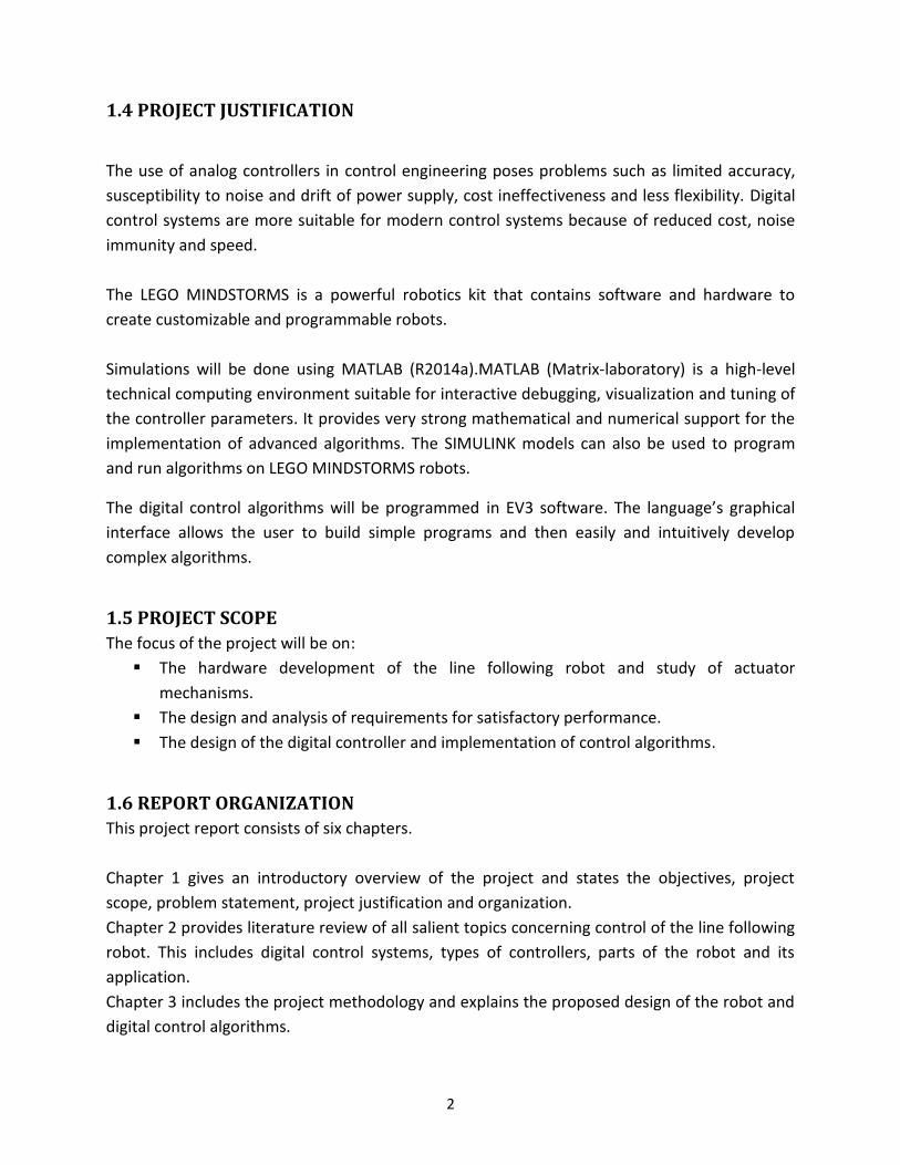
1.4 PROJECT JUSTIFICATION
The use of analog controllers in control engineering poses problems such as limited accuracy,
susceptibility to noise and drift of power supply, cost ineffectiveness and less flexibility. Digital
control systems are more suitable for modern control systems because of reduced cost, noise
immunity and speed.
The LEGO MINDSTORMS is a powerful robotics kit that contains software and hardware to
create customizable and programmable robots.
Simulations will be done using MATLAB (R2014a).MATLAB (Matrix-laboratory) is a high-level
technical computing environment suitable for interactive debugging, visualization and tuning of
the controller parameters. It provides very strong mathematical and numerical support for the
implementation of advanced algorithms. The SIMULINK models can also be used to program
and run algorithms on LEGO MINDSTORMS robots.
The digital control algorithms will be programmed in EV3 software. The language’s graphical
interface allows the user to build simple programs and then easily and intuitively develop
complex algorithms.
1.5 PROJECT SCOPE
The focus of the project will be on:
The hardware development of the line following robot and study of actuator
mechanisms.
The design and analysis of requirements for satisfactory performance.
The design of the digital controller and implementation of control algorithms.
1.6 REPORT ORGANIZATION
This project report consists of six chapters.
Chapter 1 gives an introductory overview of the project and states the objectives, project
scope, problem statement, project justification and organization.
Chapter 2 provides literature review of all salient topics concerning control of the line following
robot. This includes digital control systems, types of controllers, parts of the robot and its
application.
Chapter 3 includes the project methodology and explains the proposed design of the robot and
digital control algorithms.

3
Chapter 4 presents the analysis of the results of the project.
Chapter 5 deals with the overall conclusion, suggestions and recommendations for further
work.
Chapter 6 outlines the references cited in this project report.
4
CHAPTER 2
2. LITERATURE REVIEW
2.1 DIGITAL CONTROL SYSTEMS
2.1.1 INTRODUCTION
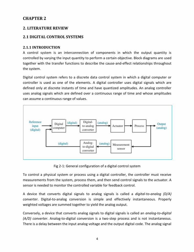
A control system is an interconnection of components in which the output quantity is
controlled by varying the input quantity to perform a certain objective. Block diagrams are used
together with the transfer functions to describe the cause-and-effect relationships throughout
the system.
Digital control system refers to a discrete data control system in which a digital computer or
controller is used as one of the elements. A digital controller uses digital signals which are
defined only at discrete instants of time and have quantized amplitudes. An analog controller
uses analog signals which are defined over a continuous range of time and whose amplitudes
can assume a continuous range of values.
Fig 2-1: General configuration of a digital control system
To control a physical system or process using a digital controller, the controller must receive
measurements from the system, process them, and then send control signals to the actuator. A
sensor is needed to monitor the controlled variable for feedback control.
A device that converts digital signals to analog signals is called a digital-to-analog (D/A)
converter. Digital-to-analog conversion is simple and effectively instantaneous. Properly
weighted voltages are summed together to yield the analog output.
Conversely, a device that converts analog signals to digital signals is called an analog-to-digital
(A/D) converter. Analog-to-digital conversion is a two-step process and is not instantaneous.
There is a delay between the input analog voltage and the output digital code. The analog signal
5
is first converted to a sampled signal at periodic intervals, held over the sampling interval, and
then converted to a sequence of binary numbers, the digital signal.
The sampling rate must be at least twice the bandwidth of the signal, or else there will be
distortion. This minimum sampling frequency is called the Nyquist sampling rate. Samples are
held over before being digitized because the (A/D) conversion occurs via digital counter, which
takes time to reach the correct digital number. Hence the constant analog voltage must be
present during the conversion process. A zero-order sample-and-hold (z.o.h) device yields a
staircase approximation to the analog system. Higher-order devices, such as a first-order hold,
generate more complex and more accurate wave shapes between the samples.
The z-transform is the principal analytical tool for analyzing sampled-data systems, and is
analogous to the Laplace transform for continuous systems. It allows sampled waveform to be
represented at the sampling instants.
2.1.2 WHY DIGITAL CONTROL?
Digital control offers distinct advantages over analog control that explain its popularity.
Speed: The increase in processing speed of computer hardware over the ages has made it
possible to sample and process control signals at very high speeds. Because the sampling
period can be made very small, digital controllers achieve performance that is essentially
the same as that based on continuous monitoring of the controlled variable.
Cost: Advances in very large-scale integration (VLSI) technology have made it possible to
manufacture better, faster, and more reliable integrated circuits. Decrease in the cost of
digital circuitry has made the use of digital controllers more economical even for small, low-
cost applications.
Accuracy: Digital signals are represented in term of zeros and ones with typically 12 bits or
more to represent a single number. This involves a very small error as compared to analog
signals, where noise and power supply drift are present.
Flexibility: An analog controller is difficult to modify or redesign once implemented in
hardware. A digital controller is implemented in firmware or software and its modification is
possible without a complete replacement of the original controller. Furthermore, the
structure of the digital controller need not follow one of the simple forms that are typically
used in analog control. More complex controller structures involve a few extra arithmetic
operations and are easily reliable.
Implementation errors. Digital processing of control signals involves addition and
multiplication by stored numerical values. The errors that result from digital representation
and arithmetic are negligible. By contrast, the processing of analog signals is performed
using components such as resistors and capacitors with actual values that vary significantly
from the nominal design values.
6
2.1.3 TYPES OF CONTROLLERS
Proportional Controller: The actuating error signal for the control signal is proportional to
the error signal. The effect on the performance of a system is that it improves the steady-
state tracking accuracy, disturbance signal rejection and relative stability of the system. It
also increases the open-loop gain of the system which results in reducing the sensitivity of
the system. Increasing the gain to very large values may lead to instability of the system.
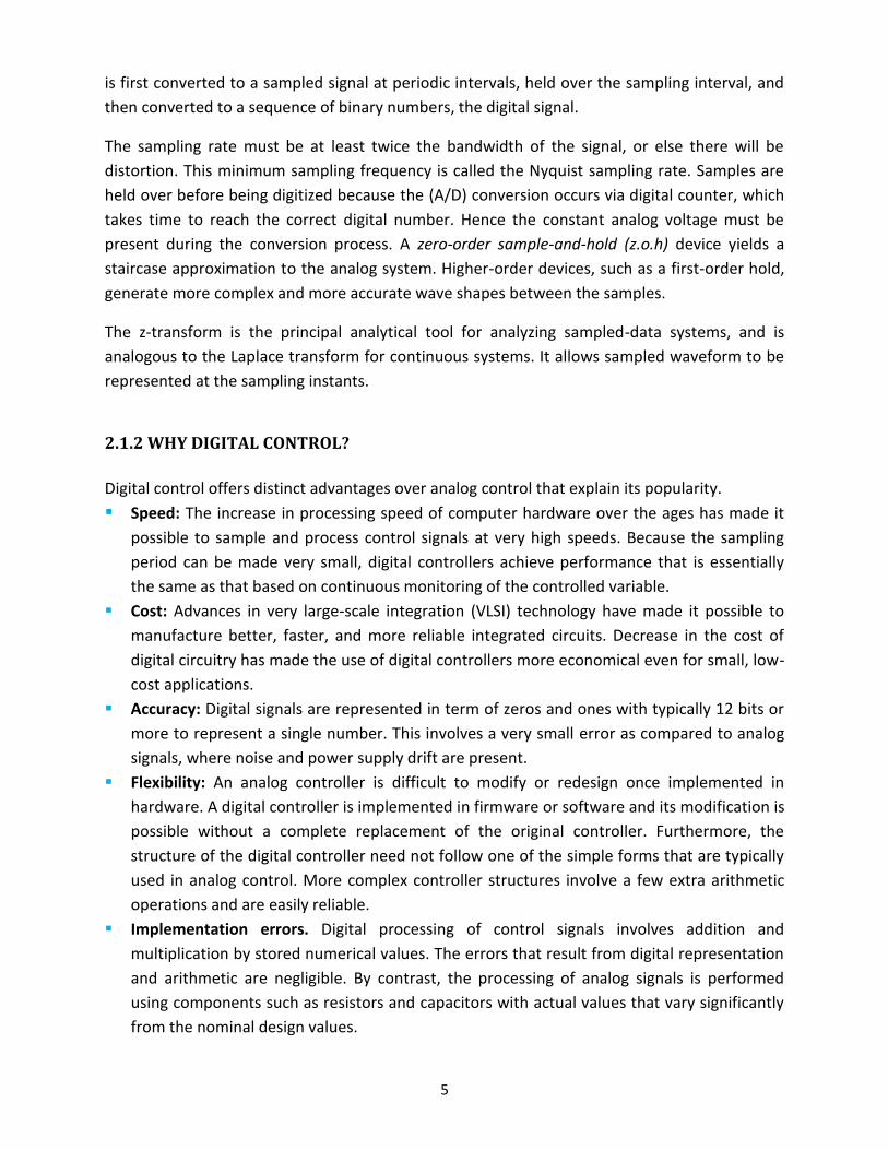
Proportional-Plus-Derivative (PD) Controller: the actuating error signal consists of
proportional error signal added to derivative of error signal. This increases the damping
ratio of the system and so the peak overshoot is reduced. Rise time and settling time are
reduced. Bandwidth is increased while the gain margin and phase margin are improved. PD
controller improves transient response.
Fig 2-2: Feedback loop with PD control
Proportional-Plus-Integral (PI) Controller: The actuating error signal consists of
proportional error signal added to the integral of error signal. It increases the order of the
system by one, which results in the reduction or removal of the steady state error. The
system becomes less stable. A properly designed PI controller decreases bandwidth but it
still improves the gain margin and phase margin.

7
Fig 2-3: Feedback loop with PI control
Proportional-Plus-Integral-Plus-Derivative (PID) Controller: This controller has the
actuating signal consisting of proportional error signal added with derivative and derivative
and integral of error signal. The combined PID control action has the advantage of each of
the three individual control actions.
Fig 2-4: Feedback loop with PID control.
2.2 LEGO MINDSTORMS EV3
The Lego Mindstorms EV3 robotics system is the third generation robot in the Lego Mindstorms
robotics line. It was released as a successor platform to the second generation Lego
Mindstorms NXT 2.0 robot.
8
2.2.1 PARTS OF THE LINE FOLLOWING ROBOT
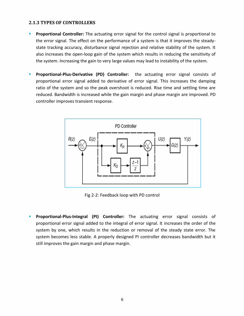
2.2.1.1. THE EV3 BRICK
The EV3 brick is an intelligent programmable microcomputer that controls the motors and
sensors, executes written programs and commands, and provides wireless communication
through Wi-Fi and Bluetooth.
A breakdown of the technical specifications of the EV3 Brick is provided in the following list:
300 MHz, ARM9 Main Microprocessor with Linux-based operating system
On-board program storage including 16 MB of Flash memory and 64 MB RAM Main
Memory
User interface with three-colour, 6 backlit buttons that indicates the brick’s active state
LCD Monochrome Display, 178 X 128 pixels
SD-Micro card reader for 32 GB of expanded memory
4 input ports (for sensors) for data acquisition of up to 1000 samples/second
4 output ports (for motors) for execution of commands
Computer-to-brick communication through on-board USB, or external Bluetooth or Wi-
Fi connection
High-quality speaker
2.2.1.2. POWER SUPPLY
Power supply provides the energy to drive the controller, sensors and actuators. The 2050
mAh Lithium-ion EV3 Rechargeable DC battery pack is the preferred power supply option.
Six AA batteries can also be used to power the robot electronic parts.
Fig 2-5: Front and back views of the EV3 Brick. The back is the 9V battery.
9
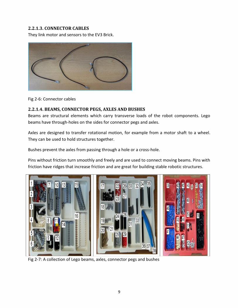
2.2.1.3. CONNECTOR CABLES
They link motor and sensors to the EV3 Brick.
Fig 2-6: Connector cables
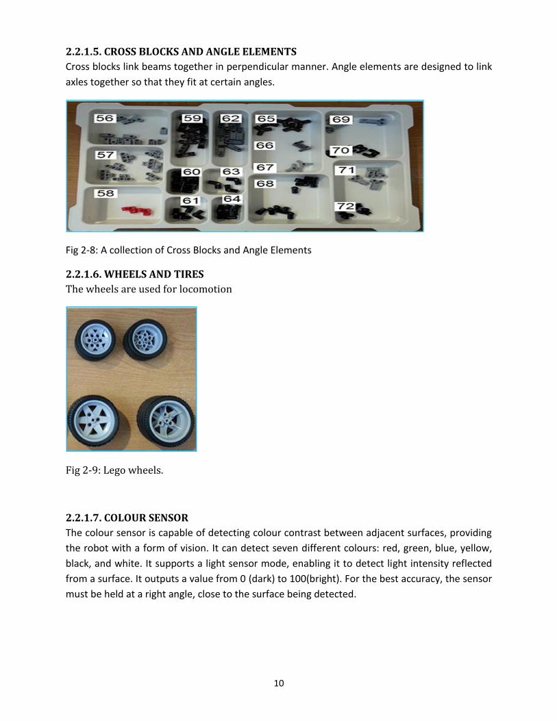
2.2.1.4. BEAMS, CONNECTOR PEGS, AXLES AND BUSHES
Beams are structural elements which carry transverse loads of the robot components. Lego
beams have through-holes on the sides for connector pegs and axles.
Axles are designed to transfer rotational motion, for example from a motor shaft to a wheel.
They can be used to hold structures together.
Bushes prevent the axles from passing through a hole or a cross-hole.
Pins without friction turn smoothly and freely and are used to connect moving beams. Pins with
friction have ridges that increase friction and are great for building stable robotic structures.
Fig 2-7: A collection of Lego beams, axles, connector pegs and bushes
10
2.2.1.5. CROSS BLOCKS AND ANGLE ELEMENTS
Cross blocks link beams together in perpendicular manner. Angle elements are designed to link
axles together so that they fit at certain angles.
Fig 2-8: A collection of Cross Blocks and Angle Elements
2.2.1.6. WHEELS AND TIRES
The wheels are used for locomotion
Fig 2-9: Lego wheels.
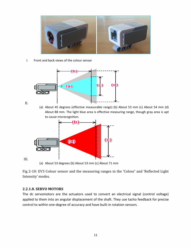
2.2.1.7. COLOUR SENSOR
The colour sensor is capable of detecting colour contrast between adjacent surfaces, providing
the robot with a form of vision. It can detect seven different colours: red, green, blue, yellow,
black, and white. It supports a light sensor mode, enabling it to detect light intensity reflected
from a surface. It outputs a value from 0 (dark) to 100(bright). For the best accuracy, the sensor
must be held at a right angle, close to the surface being detected.
11
I. Front and back views of the colour sensor
II. (a) About 45 degrees (effective measurable range) (b) About 53 mm (c) About 54 mm (d)
About 88 mm. The light blue area is effective measuring range, though gray area is apt
to cause misrecognition.
III. (a) About 53 degrees (b) About 53 mm (c) About 71 mm
Fig 2-10: EV3 Colour sensor and the measuring ranges in the ‘Colour’ and ‘Reflected Light
Intensity’ modes.
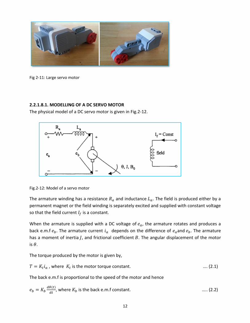
2.2.1.8. SERVO MOTORS
The dc servomotors are the actuators used to convert an electrical signal (control voltage)
applied to them into an angular displacement of the shaft. They use tacho feedback for precise
control to within one-degree of accuracy and have built-in rotation sensors.
12
Fig 2-11: Large servo motor
2.2.1.8.1. MODELLING OF A DC SERVO MOTOR
The physical model of a DC servo motor is given in Fig.2-12.
Fig.2-12: Model of a servo motor
The armature winding has a resistance and inductance . The field is produced either by a
permanent magnet or the field winding is separately excited and supplied with constant voltage
so that the field current is a constant.
When the armature is supplied with a DC voltage of , the armature rotates and produces a
back e.m.f . The armature current depends on the difference of and . The armature
has a moment of inertia , and frictional coefficient . The angular displacement of the motor
is .
The torque produced by the motor is given by,
, where is the motor torque constant. …. (2.1)
The back e.m.f is proportional to the speed of the motor and hence
, where is the back e.m.f constant. ….. (2.2)
13
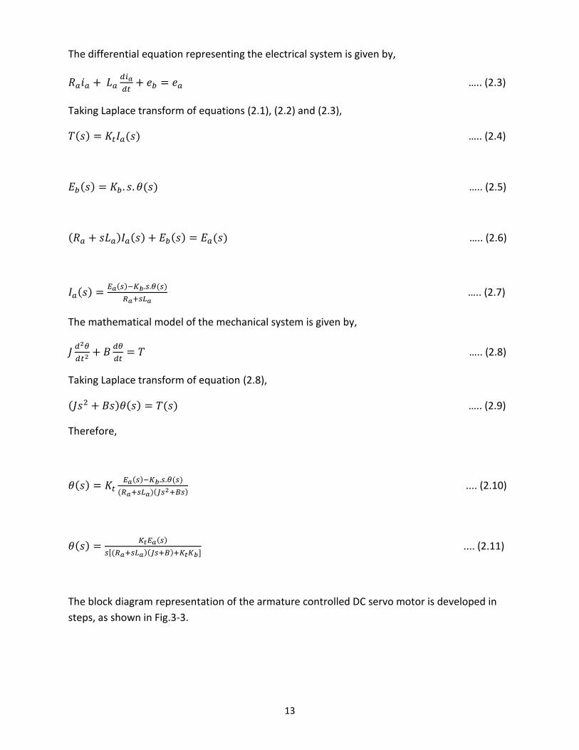
The differential equation representing the electrical system is given by,
….. (2.3)
Taking Laplace transform of equations (2.1), (2.2) and (2.3),
….. (2.4)
….. (2.5)
….. (2.6)
….. (2.7)
The mathematical model of the mechanical system is given by,
….. (2.8)
Taking Laplace transform of equation (2.8),
….. (2.9)
Therefore,
.... (2.10)
[ .... (2.11)
The block diagram representation of the armature controlled DC servo motor is developed in
steps, as shown in Fig.3-3.
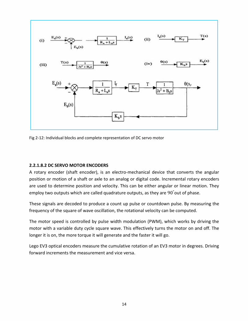
14
Fig 2-12: Individual blocks and complete representation of DC servo motor
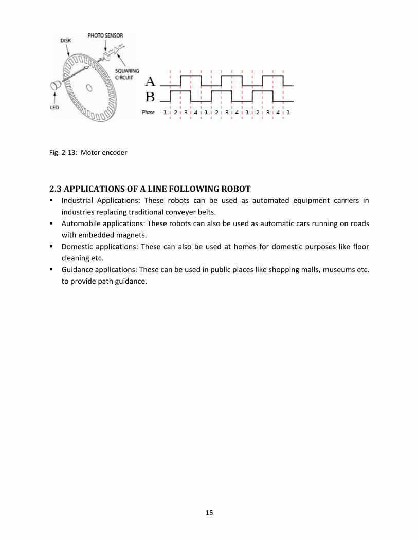
2.2.1.8.2 DC SERVO MOTOR ENCODERS
A rotary encoder (shaft encoder), is an electro-mechanical device that converts the angular
position or motion of a shaft or axle to an analog or digital code. Incremental rotary encoders
are used to determine position and velocity. This can be either angular or linear motion. They
employ two outputs which are called quadrature outputs, as they are out of phase.
These signals are decoded to produce a count up pulse or countdown pulse. By measuring the
frequency of the square of wave oscillation, the rotational velocity can be computed.
The motor speed is controlled by pulse width modulation (PWM), which works by driving the
motor with a variable duty cycle square wave. This effectively turns the motor on and off. The
longer it is on, the more torque it will generate and the faster it will go.
Lego EV3 optical encoders measure the cumulative rotation of an EV3 motor in degrees. Driving
forward increments the measurement and vice versa.
15
Fig. 2-13: Motor encoder
2.3 APPLICATIONS OF A LINE FOLLOWING ROBOT
Industrial Applications: These robots can be used as automated equipment carriers in
industries replacing traditional conveyer belts.
Automobile applications: These robots can also be used as automatic cars running on roads
with embedded magnets.
Domestic applications: These can also be used at homes for domestic purposes like floor
cleaning etc.
Guidance applications: These can be used in public places like shopping malls, museums etc.
to provide path guidance.
16
CHAPTER 3
3. METHODOLOGY
The design of the digital controller for a line following robotic was done in stages.
Design and construction of a robot that can follow a line using Lego Mindstorms EV3.
Development of line following algorithms.
Study of the response of the LFR.
Design of a P.I.D digital controller to ensure satisfactory control of the system
Implementation of the whole control algorithm on EV3 hardware
Study of the performance of the compensated system
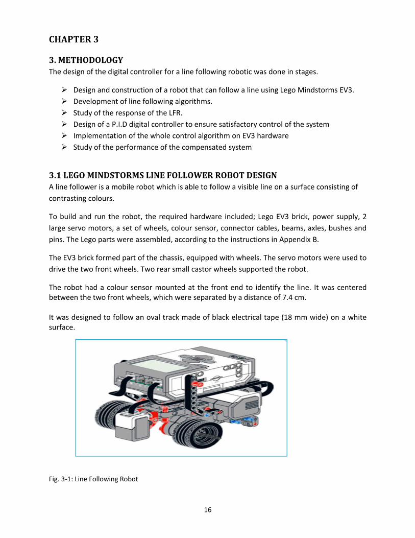
3.1 LEGO MINDSTORMS LINE FOLLOWER ROBOT DESIGN
A line follower is a mobile robot which is able to follow a visible line on a surface consisting of
contrasting colours.
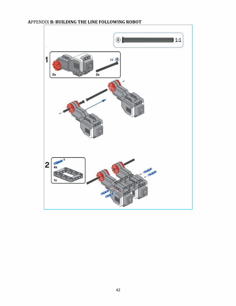
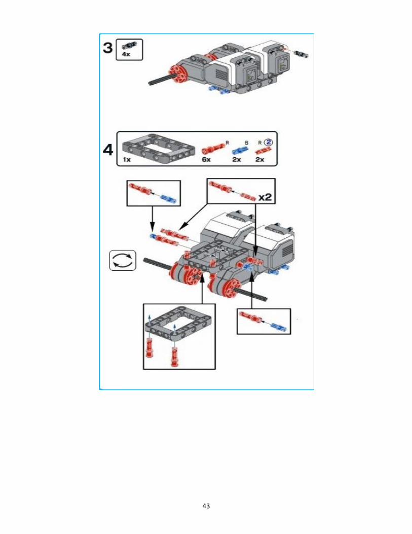
To build and run the robot, the required hardware included; Lego EV3 brick, power supply, 2
large servo motors, a set of wheels, colour sensor, connector cables, beams, axles, bushes and
pins. The Lego parts were assembled, according to the instructions in Appendix B.
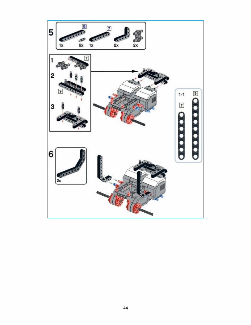
The EV3 brick formed part of the chassis, equipped with wheels. The servo motors were used to
drive the two front wheels. Two rear small castor wheels supported the robot.
The robot had a colour sensor mounted at the front end to identify the line. It was centered between the two front wheels, which were separated by a distance of 7.4 cm. It was designed to follow an oval track made of black electrical tape (18 mm wide) on a white surface.
Fig. 3-1: Line Following Robot
17
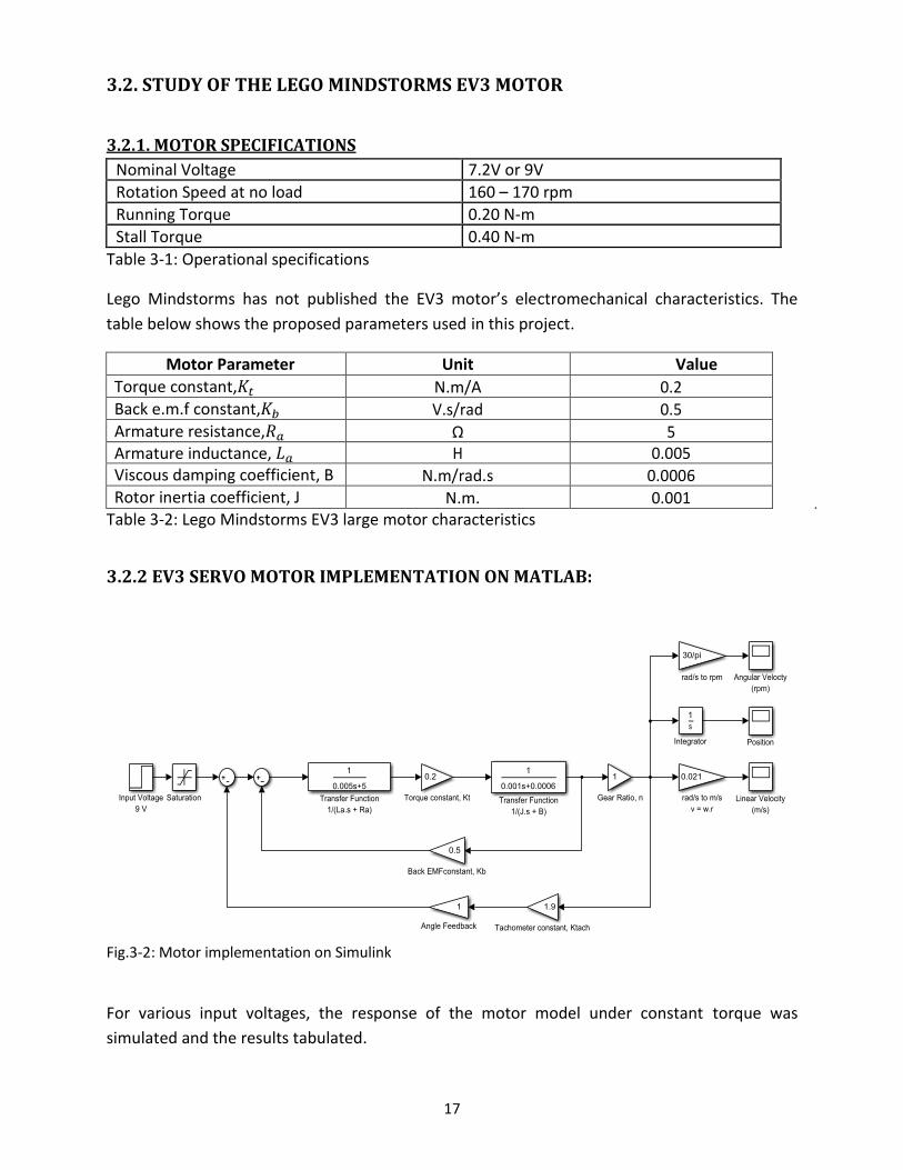
3.2. STUDY OF THE LEGO MINDSTORMS EV3 MOTOR
3.2.1. MOTOR SPECIFICATIONS
Nominal Voltage 7.2V or 9V
Rotation Speed at no load 160 – 170 rpm
Running Torque 0.20 N-m
Stall Torque 0.40 N-m
Table 3-1: Operational specifications
Lego Mindstorms has not published the EV3 motor’s electromechanical characteristics. The
table below shows the proposed parameters used in this project.
Motor Parameter Unit Value
Torque constant, N.m/A 0.2
Back e.m.f constant, V.s/rad 0.5
Armature resistance, Ω 5
Armature inductance, H 0.005
Viscous damping coefficient, B N.m/rad.s 0.0006
Rotor inertia coefficient, J N.m. 0.001
Table 3-2: Lego Mindstorms EV3 large motor characteristics
3.2.2 EV3 SERVO MOTOR IMPLEMENTATION ON MATLAB:
Fig.3-2: Motor implementation on Simulink
For various input voltages, the response of the motor model under constant torque was
simulated and the results tabulated.
18
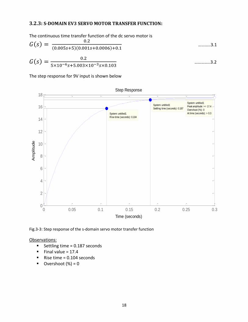
3.2.3: S-DOMAIN EV3 SERVO MOTOR TRANSFER FUNCTION:
The continuous time transfer function of the dc servo motor is
………..3.1
…………..3.2
The step response for 9V input is shown below
Fig.3-3: Step response of the s-domain servo motor transfer function
Observations: Settling time = 0.187 seconds Final value = 17.4 Rise time = 0.104 seconds Overshoot (%) = 0
Step Response
Time (seconds)
Am
plitu
de
0 0.05 0.1 0.15 0.2 0.25 0.30
2
4
6
8
10
12
14
16
18
System: untitled1
Settling time (seconds): 0.187
System: untitled1
Peak amplitude: >= 17.4
Overshoot (%): 0
At time (seconds): > 0.3System: untitled1
Rise time (seconds): 0.104
19
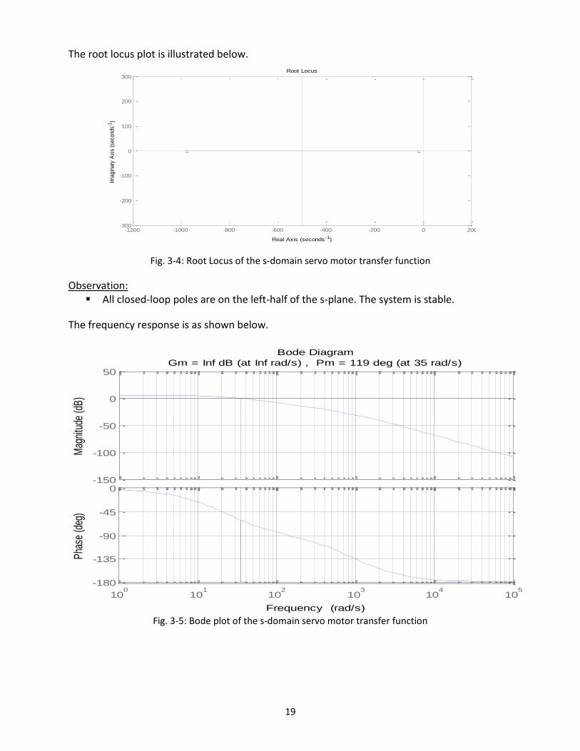
The root locus plot is illustrated below.
Fig. 3-4: Root Locus of the s-domain servo motor transfer function
Observation: All closed-loop poles are on the left-half of the s-plane. The system is stable.
The frequency response is as shown below.
Fig. 3-5: Bode plot of the s-domain servo motor transfer function
-1200 -1000 -800 -600 -400 -200 0 200-300
-200
-100
0
100
200
300Root Locus
Real Axis (seconds-1)
Imag
inar
y A
xis
(sec
onds
-1)
-150
-100
-50
0
50
Mag
nitu
de (d
B)
100
101
102
103
104
105
-180
-135
-90
-45
0
Pha
se (d
eg)
Bode Diagram
Gm = Inf dB (at Inf rad/s) , Pm = 119 deg (at 35 rad/s)
Frequency (rad/s)
20
Observations: Gain margin is infinite
Phase margin is
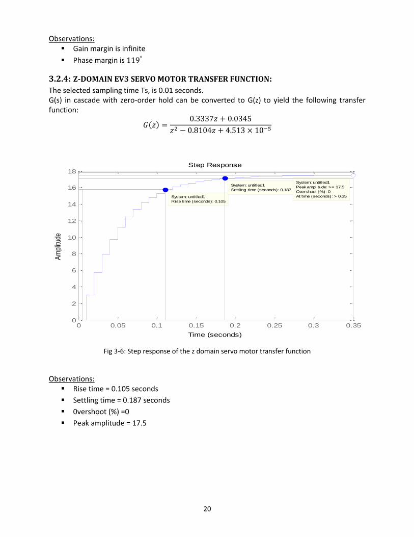
3.2.4: Z-DOMAIN EV3 SERVO MOTOR TRANSFER FUNCTION:
The selected sampling time Ts, is 0.01 seconds. G(s) in cascade with zero-order hold can be converted to G(z) to yield the following transfer function:
Fig 3-6: Step response of the z domain servo motor transfer function
Observations:
Rise time = 0.105 seconds
Settling time = 0.187 seconds
0vershoot (%) =0
Peak amplitude = 17.5
Step Response
Time (seconds)
Am
plitu
de
0 0.05 0.1 0.15 0.2 0.25 0.3 0.350
2
4
6
8
10
12
14
16
18
System: untitled1
Rise time (seconds): 0.105
System: untitled1
Settling time (seconds): 0.187
System: untitled1
Peak amplitude: >= 17.5
Overshoot (%): 0
At time (seconds): > 0.35
21
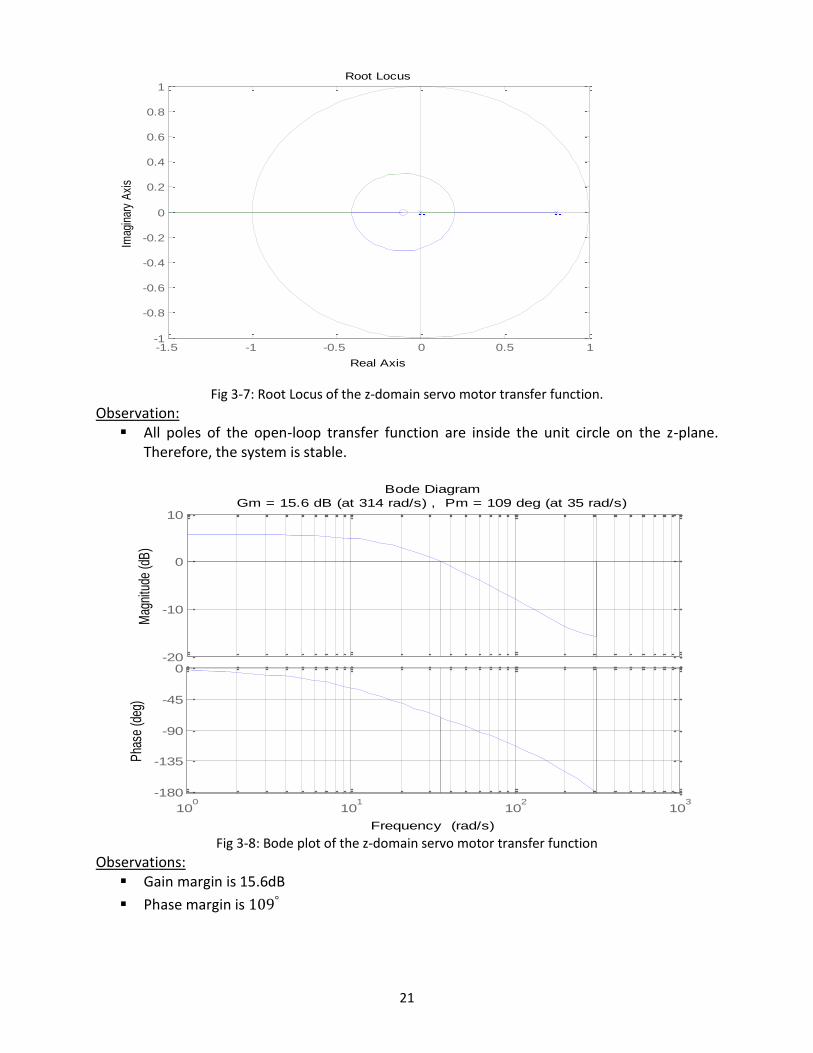
Fig 3-7: Root Locus of the z-domain servo motor transfer function.
Observation: All poles of the open-loop transfer function are inside the unit circle on the z-plane.
Therefore, the system is stable.
Fig 3-8: Bode plot of the z-domain servo motor transfer function
Observations: Gain margin is 15.6dB
Phase margin is
-1.5 -1 -0.5 0 0.5 1-1
-0.8
-0.6
-0.4
-0.2
0
0.2
0.4
0.6
0.8
1Root Locus
Real Axis
Imag
inar
y A
xis
-20
-10
0
10
Mag
nitu
de (d
B)
100
101
102
103
-180
-135
-90
-45
0
Pha
se (d
eg)
Bode Diagram
Gm = 15.6 dB (at 314 rad/s) , Pm = 109 deg (at 35 rad/s)
Frequency (rad/s)
22
3.3 LINE FOLLOWING ROBOT ALGORITHMS
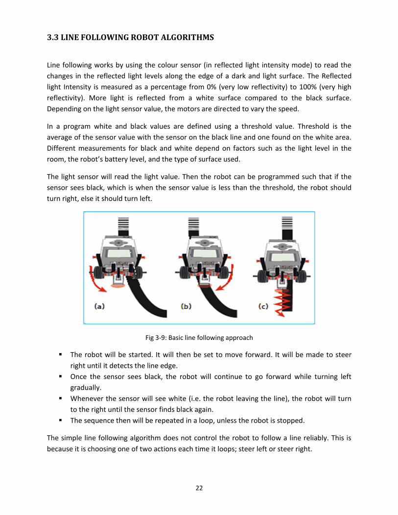
Line following works by using the colour sensor (in reflected light intensity mode) to read the
changes in the reflected light levels along the edge of a dark and light surface. The Reflected
light Intensity is measured as a percentage from 0% (very low reflectivity) to 100% (very high
reflectivity). More light is reflected from a white surface compared to the black surface.
Depending on the light sensor value, the motors are directed to vary the speed.
In a program white and black values are defined using a threshold value. Threshold is the
average of the sensor value with the sensor on the black line and one found on the white area.
Different measurements for black and white depend on factors such as the light level in the
room, the robot’s battery level, and the type of surface used.
The light sensor will read the light value. Then the robot can be programmed such that if the
sensor sees black, which is when the sensor value is less than the threshold, the robot should
turn right, else it should turn left.
Fig 3-9: Basic line following approach
The robot will be started. It will then be set to move forward. It will be made to steer
right until it detects the line edge.
Once the sensor sees black, the robot will continue to go forward while turning left
gradually.
Whenever the sensor will see white (i.e. the robot leaving the line), the robot will turn
to the right until the sensor finds black again.
The sequence then will be repeated in a loop, unless the robot is stopped.
The simple line following algorithm does not control the robot to follow a line reliably. This is
because it is choosing one of two actions each time it loops; steer left or steer right.
23
3.4: DIGITAL CONTROLLER DESIGN: A robot without a controller will oscillate a lot about the line, leading to more consumption of battery power, less speed and following the line less efficiently.
When designing a line following robot, the transient response specifications are defined as: Rise time: It is how fast the robot will try to get back to the line after it has drifted off.
Overshoot: The distance past the line edge the robot will tend to go as it is responding to an
error. The amount of overshoot indicates the relative stability of the system.
Steady-state error: the offset from the line as the robot follows a long straight line.
Settling time: The time the LFR will take to settle down when it encounters a turn.
The performance criteria were stipulated as follows: Constant speed of 0.1m/s to be maintained despite the presence of turns.
Steady-state error: Less than 2%
Settling time of less than 0.1 seconds
Overshoot (%) of less than 1.0
Finite phase margin
The robot controller to be designed was to be modified until the transient response met was satisfactory.
3.4.1. PROPOSED CONTROLLER DESIGN:
The proposed controller was a Proportional-plus-Integral-plus-Derivative (PID) digital controller.
The PID controller would control the position of the robot with quick response time and minimize the overshoot.
The proportional part would determine the magnitude of turn required to correct the error sensed.
The integral part would improve the steady state error (proportional offset) which increases while the robot is not on the line. The derivative part would measure the deviation from the path and minimize overshoot. It would reduce the oscillating effect about the line. The derivative control is used to provide anticipative action.
24
3.4.2: IMPLEMENTATION OF LINE FOLLOWING CONTROL ALGORITHM FOR THE LEGO
MINDSTORMS EV3 HARDWARE:
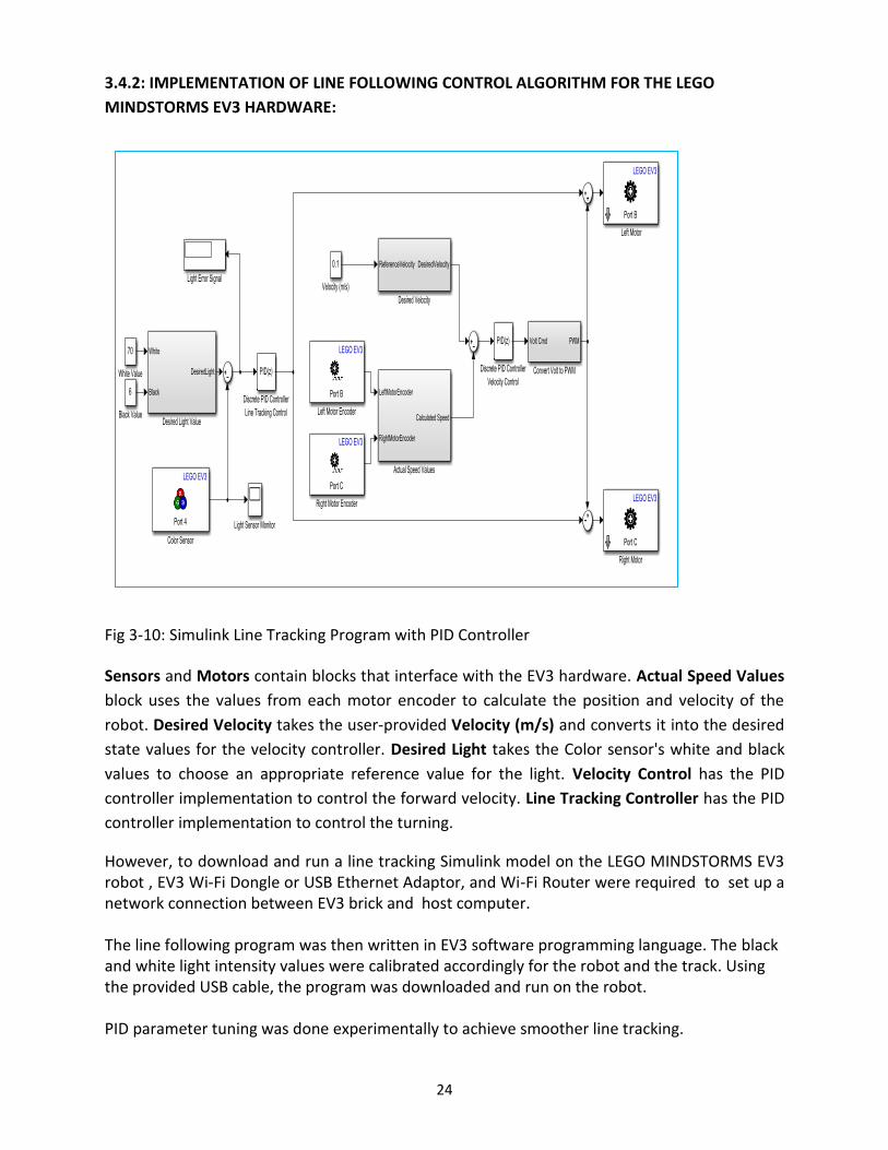
Fig 3-10: Simulink Line Tracking Program with PID Controller
Sensors and Motors contain blocks that interface with the EV3 hardware. Actual Speed Values
block uses the values from each motor encoder to calculate the position and velocity of the
robot. Desired Velocity takes the user-provided Velocity (m/s) and converts it into the desired
state values for the velocity controller. Desired Light takes the Color sensor's white and black
values to choose an appropriate reference value for the light. Velocity Control has the PID
controller implementation to control the forward velocity. Line Tracking Controller has the PID
controller implementation to control the turning.
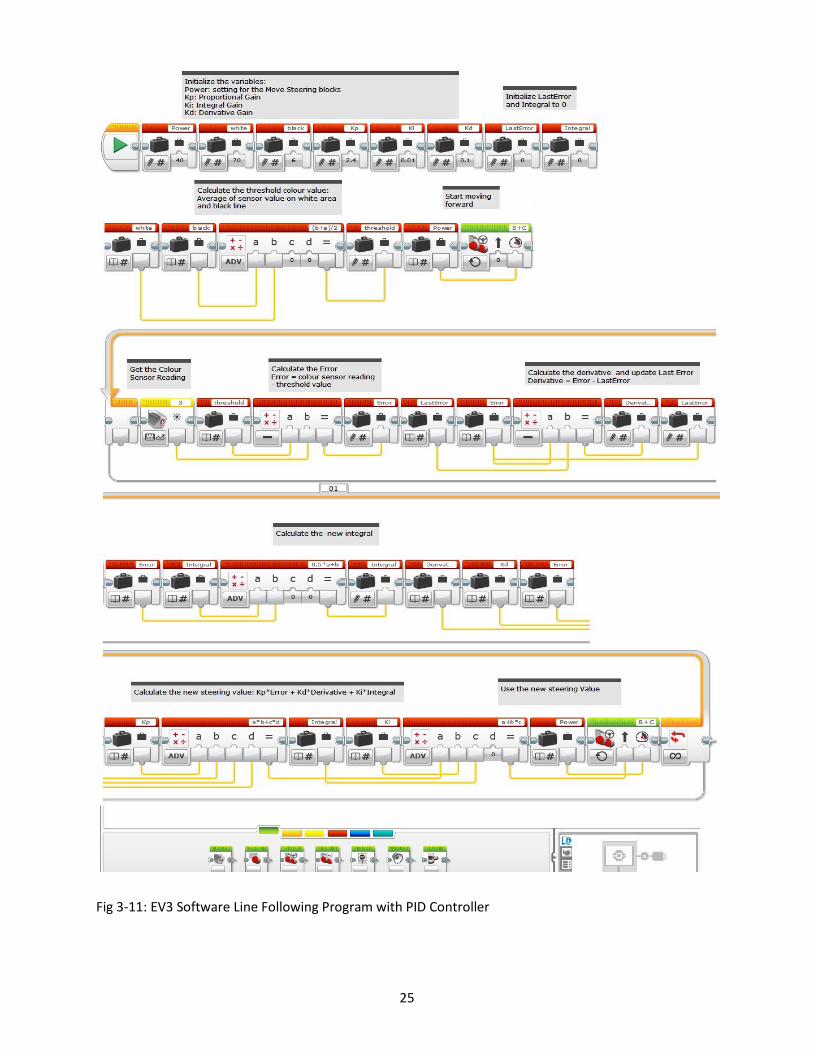
However, to download and run a line tracking Simulink model on the LEGO MINDSTORMS EV3 robot , EV3 Wi-Fi Dongle or USB Ethernet Adaptor, and Wi-Fi Router were required to set up a network connection between EV3 brick and host computer. The line following program was then written in EV3 software programming language. The black and white light intensity values were calibrated accordingly for the robot and the track. Using the provided USB cable, the program was downloaded and run on the robot. PID parameter tuning was done experimentally to achieve smoother line tracking.
25
Fig 3-11: EV3 Software Line Following Program with PID Controller
26
CHAPTER 4
4. RESULTS AND ANALYSIS
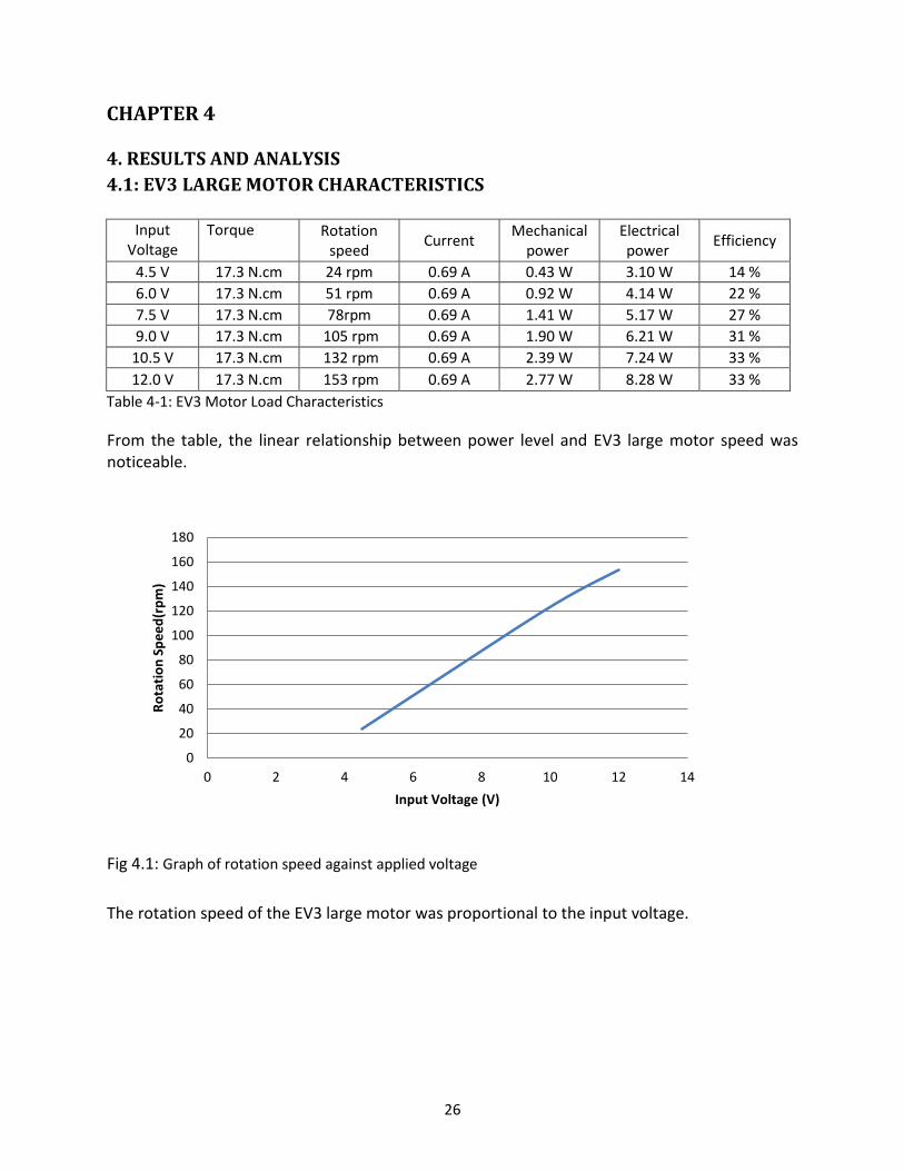
4.1: EV3 LARGE MOTOR CHARACTERISTICS
Input Voltage
Torque Rotation speed
Current Mechanical
power Electrical power
Efficiency
4.5 V 17.3 N.cm 24 rpm 0.69 A 0.43 W 3.10 W 14 %
6.0 V 17.3 N.cm 51 rpm 0.69 A 0.92 W 4.14 W 22 %
7.5 V 17.3 N.cm 78rpm 0.69 A 1.41 W 5.17 W 27 %
9.0 V 17.3 N.cm 105 rpm 0.69 A 1.90 W 6.21 W 31 %
10.5 V 17.3 N.cm 132 rpm 0.69 A 2.39 W 7.24 W 33 %
12.0 V 17.3 N.cm 153 rpm 0.69 A 2.77 W 8.28 W 33 %
Table 4-1: EV3 Motor Load Characteristics
From the table, the linear relationship between power level and EV3 large motor speed was noticeable.
Fig 4.1: Graph of rotation speed against applied voltage The rotation speed of the EV3 large motor was proportional to the input voltage.
0
20
40
60
80
100
120
140
160
180
0 2 4 6 8 10 12 14
Ro
tati
on
Sp
ee
d(r
pm
)
Input Voltage (V)
27
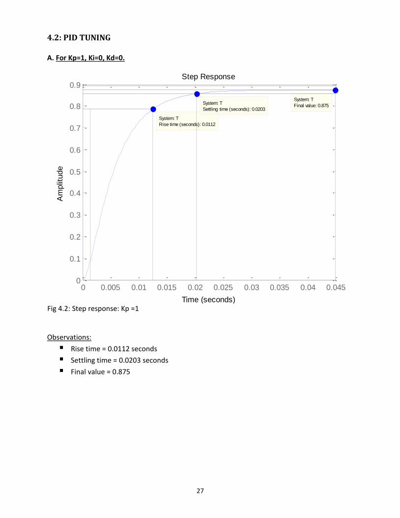
4.2: PID TUNING
A. For Kp=1, Ki=0, Kd=0.
Fig 4.2: Step response: Kp =1 Observations:
Rise time = 0.0112 seconds Settling time = 0.0203 seconds Final value = 0.875
Step Response
Time (seconds)
Am
plit
ude
0 0.005 0.01 0.015 0.02 0.025 0.03 0.035 0.04 0.0450
0.1
0.2
0.3
0.4
0.5
0.6
0.7
0.8
0.9
System: T
Rise time (seconds): 0.0112
System: T
Settling time (seconds): 0.0203
System: T
Final value: 0.875
28
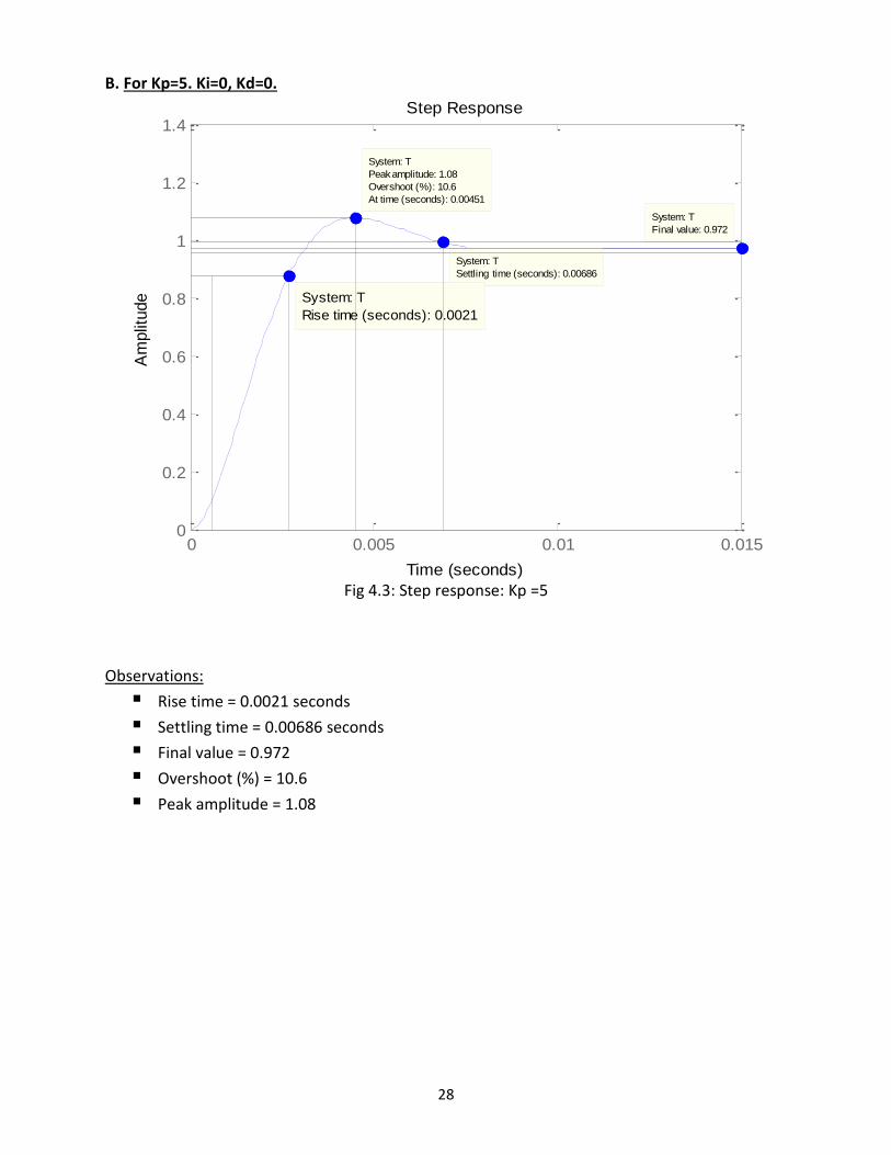
B. For Kp=5. Ki=0, Kd=0.
Fig 4.3: Step response: Kp =5
Observations:
Rise time = 0.0021 seconds Settling time = 0.00686 seconds Final value = 0.972 Overshoot (%) = 10.6 Peak amplitude = 1.08
Step Response
Time (seconds)
Am
plit
ude
0 0.005 0.01 0.0150
0.2
0.4
0.6
0.8
1
1.2
1.4
System: T
Final value: 0.972
System: T
Settling time (seconds): 0.00686
System: T
Peak amplitude: 1.08
Overshoot (%): 10.6
At time (seconds): 0.00451
System: T
Rise time (seconds): 0.0021
29
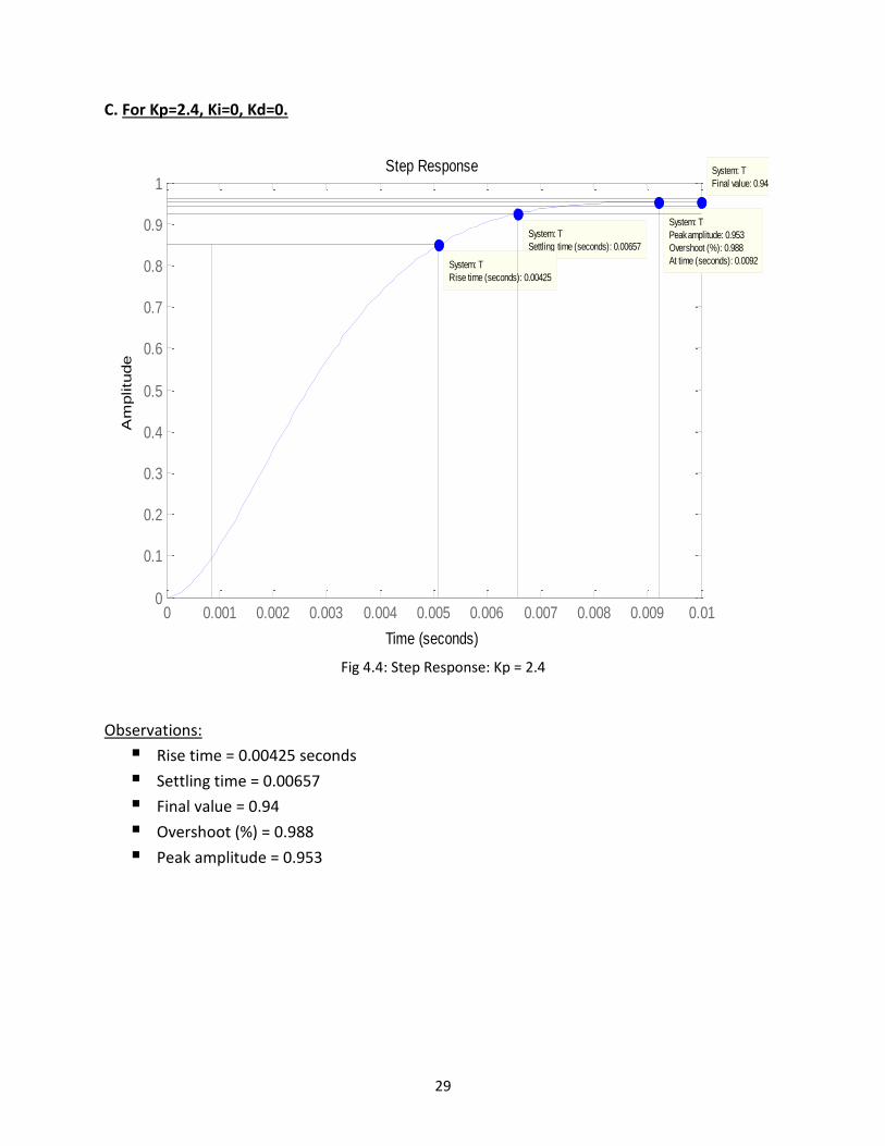
C. For Kp=2.4, Ki=0, Kd=0.
Fig 4.4: Step Response: Kp = 2.4
Observations:
Rise time = 0.00425 seconds Settling time = 0.00657 Final value = 0.94 Overshoot (%) = 0.988 Peak amplitude = 0.953
Step Response
Time (seconds)
Am
plitu
de
0 0.001 0.002 0.003 0.004 0.005 0.006 0.007 0.008 0.009 0.010
0.1
0.2
0.3
0.4
0.5
0.6
0.7
0.8
0.9
1System: T
Final value: 0.944
System: T
Peak amplitude: 0.953
Overshoot (%): 0.988
At time (seconds): 0.0092
System: T
Settling time (seconds): 0.00657
System: T
Rise time (seconds): 0.00425
30
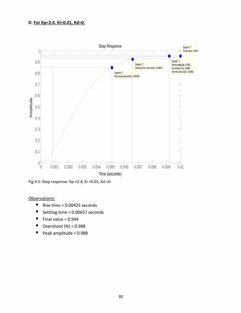
D. For Kp=2.4. Ki=0.01, Kd=0.
Fig 4.5: Step response: Kp =2.4, Ki =0.01, Kd =0
Observations:
Rise time = 0.00425 seconds Settling time = 0.00657 seconds Final value = 0.944 Overshoot (%) = 0.988 Peak amplitude = 0.988
Step Response
Time (seconds)
Am
plitu
de
0 0.001 0.002 0.003 0.004 0.005 0.006 0.007 0.008 0.009 0.010
0.1
0.2
0.3
0.4
0.5
0.6
0.7
0.8
0.9
1
System: T
Rise time (seconds): 0.00425
System: T
Settling time (seconds): 0.00657
System: T
Peak amplitude: 0.953
Overshoot (%): 0.988
At time (seconds): 0.0092
System: T
Final value: 0.944
31
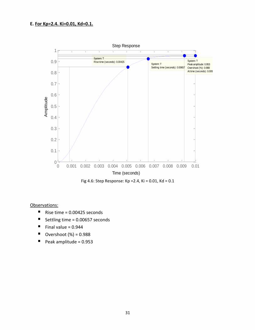
E. For Kp=2.4. Ki=0.01, Kd=0.1.
Fig 4.6: Step Response: Kp =2.4, Ki = 0.01, Kd = 0.1
Observations:
Rise time = 0.00425 seconds Settling time = 0.00657 seconds Final value = 0.944 Overshoot (%) = 0.988 Peak amplitude = 0.953
Step Response
Time (seconds)
Am
plitu
de
0 0.001 0.002 0.003 0.004 0.005 0.006 0.007 0.008 0.009 0.010
0.1
0.2
0.3
0.4
0.5
0.6
0.7
0.8
0.9
1
System: T
Rise time (seconds): 0.00425 System: T
Peak amplitude: 0.953
Overshoot (%): 0.988
At time (seconds): 0.0092
System: T
Settling time (seconds): 0.00657
32
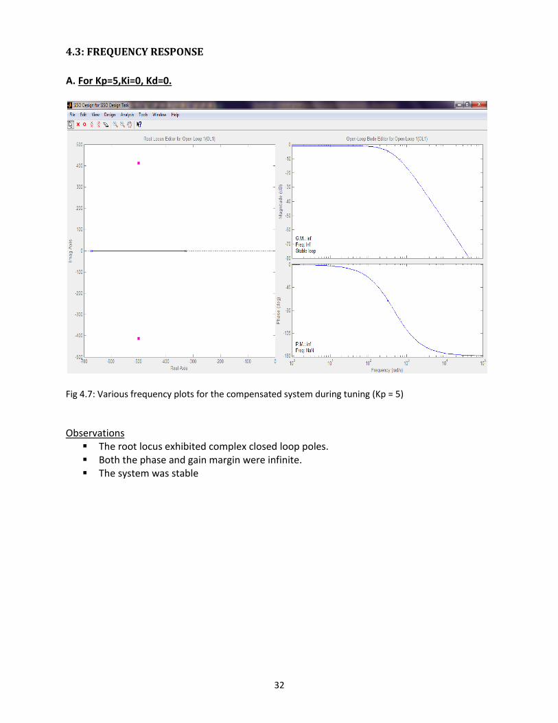
4.3: FREQUENCY RESPONSE
A. For Kp=5,Ki=0, Kd=0.
Fig 4.7: Various frequency plots for the compensated system during tuning (Kp = 5)
Observations
The root locus exhibited complex closed loop poles. Both the phase and gain margin were infinite. The system was stable
33
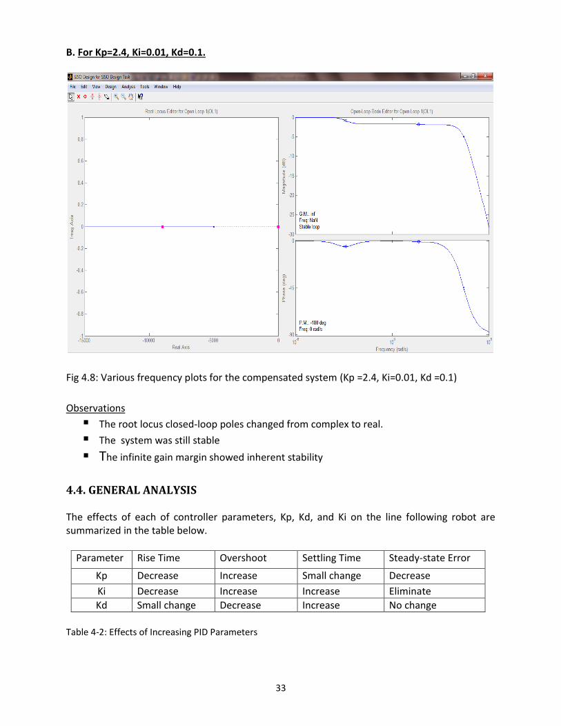
B. For Kp=2.4, Ki=0.01, Kd=0.1.
Fig 4.8: Various frequency plots for the compensated system (Kp =2.4, Ki=0.01, Kd =0.1)
Observations
The root locus closed-loop poles changed from complex to real. The system was still stable The infinite gain margin showed inherent stability
4.4. GENERAL ANALYSIS The effects of each of controller parameters, Kp, Kd, and Ki on the line following robot are summarized in the table below.
Parameter Rise Time Overshoot Settling Time Steady-state Error
Kp Decrease Increase Small change Decrease
Ki Decrease Increase Increase Eliminate
Kd Small change Decrease Increase No change
Table 4-2: Effects of Increasing PID Parameters
34
The difficulty of tuning increased with the number of parameters that were to be adjusted. To
observe the response that resulted from the tuning adjustments, it was necessary to wait for
several minutes. This made the tuning by trial-and-error a tedious and time-consuming task.
In practice, the stability of a mathematical model was not sufficient to guarantee acceptable
system performance or even to guarantee the stability of the physical system that the model
represented. This is because of the approximate nature of mathematical models.
The main problems associated with the implementation of digital control are related to the
effects of quantization and sampling.
i. Quantization effects: The conversion of signals from analog into digital form and vice-versa
is performed by electronic devices of finite resolution. A device of n-bit resolution has
quantization levels. Here, the analog signals get tied to these finite number of quantization
levels in the process of conversion to digital form. Therefore, by the sheer act of conversion
a valuable part of information about the signal is lost. Furthermore, any computer
employed as a real-time controller must perform all the necessary calculations with limited
precision, thus introducing a truncation error after each arithmetic operation has been
performed. As the computational accuracy is normally much higher than the resolution of
real converters, a further truncation must take place before the computed data is converted
into the analog form.
ii. Sampling effects: The sampling theorem ensures that there is no loss of information due to
sampling and the continuous time signal can be completely recovered from its samples
using an ideal low-pass filter. There are, however, two problems associated with the use of
this theorem in practical control systems. Real signals are not band-limited and hence strict
bandwidth limits are not defined. The ideal-low pass filter, needed for the distortionless
reconstruction of continuous-time signals from its samples, is not physically realizable.
Practical devices, such as the D/A converters, introduce distortions. Thus the process of
sampling and reconstruction also affects the amount of information available to the control
computer, and degrades control system.
The advantages of digital control outweigh its implementation problems for most of the applications.
35
CHAPTER 5
5. CONCLUSION AND RECOMMENDATIONS
5.1 CONCLUSION
A line following robot was designed and built using LEGO MINDSTORMS EV3 components.
Digital control algorithms were developed. The advantages and limitations of implementing the
digital control on different software were studied. The effectiveness of using PID controller for
optimum line tracking was demonstrated by inspecting the movement pattern of the robot
while following the track. To obtain the desired control response, Kp, Ki and Kd were
successfully determined by tuning.
5.2 RECOMMENDATIONS FOR IMPLEMENTATION
For easy navigation on various terrains, additional features will be required. Replacement of
tires with treads should be considered. Walking robots have better mobility than wheeled
robots.
Greater efficiency can be obtained if a control algorithm for obstacle avoidance is also
included. Detecting obstacles ensures the reliable and safe movement of the robot.
A convenient and economical alternative to the AA batteries is the EV3 Rechargeable
Battery. It can be recharged while inbuilt in a model, eliminating the problem of
disassembling and reassembling a robot to replace batteries. It also weighs less.
Programming languages such as C and Java can also be used to implement control
algorithms on EV3 hardware. RobotC is a C-based cross-robotics programming platform
while LeJOS allows Lego Mindstorms robots to be programmed in the Java programming
language.
To provide a valuable and highly interactive insight into the real-time internal working of
the model, Simulink is appropriate.
5.3 RECOMMENDATIONS FOR FURTHER WORK
Designing a controller required the kinematic modeling, which is a much less accurate depiction
of the actual system. The influence of the robot’s dynamics should not be neglected. Dynamic
modeling takes into account such factors such as the robot’s weight, center of gravity,
cornering stiffness, tire slippage and aerodynamic resistance. There may be complexity
encountered while deriving and working with the necessary equations and measuring some of
the parameters. However, it gives a highly accurate portrayal of the robot’s behavior.
There has been much research in the area of control theory and many modern controllers have been developed as a result. The same study of the line following robot may be done using fuzzy logic controllers, neural networks and adaptive controllers.
36
CHAPTER 6
6 REFERENCES
Daniele Benedetelli, “The Lego Mindstorms EV3 Laboratory”, No Starch Press Inc., 2014
Laurens Valk, “The Lego Mindstorms EV3 Discovery Book”, No Starch Press Inc., 2014
Terry Griffin, “The Art of Lego Mindstorms EV3 Programming”, No Starch Press Inc., 2014
Mark Rollins, “Beginning Lego Mindstorms EV3”, APress, 2014
William S. Levie, “Control System Fundamentals”, CRC Press, 1999
Jagan, N.C., “Control Systems”, BS Publications, 2008, Second Edition
Norman S. Nise, Control systems Engineering, Sixth Edition, John Wiley& Sons, Inc, 2011
Katsuhiko Ogata, “Discrete time control systems”, Prentice-Hall Inc. A Pearson Education Company, Upper Saddle River, New Jersey 07458, 1995 Kuo, B.C., “Digital Control Systems”, Saunders, 1992 R. C. Dorf and R. H. Bishop, “Modern Control Systems”, Pearson Education, Inc., Upper Saddle River, New Jersey 07458, Twelfth Edition, 2011 Jones, J., Flynn, A., Seiger, B., “Mobile Robots: From Inspiration to Implementation, A.K Peters,
Welleslay MA, 1999, Second Edition
Thomas Brӓunl, “Embedded Robotics: Mobile Robot Design and Applications with Embedded
Systems”, Springer-Verlag Berlin Heidelberg, Third Edition
Chen, C.T., Analog and Digital Control System Design, Saunders-HBJ, 1993
M. Sami Fadali, Antonio Visioli, “Digital Control Engineering: Analysis and Design”,
Academic Press- an imprint of Elsevier 30 Corporate Drive, Suite Burlington, MA 01803, 2003,
Second Edition
Lego Mindstorms EV3 [online] Available FTP: http://www.lego.com/
Lego Mindstorms EV3 – Wikipedia [online] Available FTP:
http://www.en.wikipedia.org/wiki/Lego_Mindstorms_EV3/
Lego Mindstorms - Wikipedia [online] Available FTP:
http://www.en.wikipedia.org/wiki/Lego_Mindstorms
37
Encoders [online] Available FTP: http://www.brickengineer.com/pages/2008/09/05/lego-nxt-
motor-wiring/
EV3 Color Sensor [online] Available FTP: http://www.cdstem.wordpress.com//2014/05/09/
EV3 Large Motor [online] Available FTP: http://www.afrel.co.jp.en/archives/96
Mathworks Support for Lego Mindstorms EV3 [online] Available FTP:
http://www.mathworks.com.academia/lego_mindstorms_ev3_software/
Control Tutorial for MATLAB and SIMULINK [online] Available
FTP:http://www.ctms.engin.umich.edu/
Line tracking [online] Available FTP:
http://www.mathworks.com/help/supportpkg/legomindstormsev3/examples/line-
tracking.html
Robotics [online] Available FTP: http://www.whatis.techtarget.com/definition/robotics
How to create a line following robot using Mindstorms [online] Available FTP:
http://www.thetechnicgear.com/2014/03/how_to_create_line_following_robot_using_mindst
orms/
PID Controller for Lego Mindstorms Robots [online] Available FTP:
http://www.inpharmix.com/jps/PID_Controller_For_Lego_Mindstorms_Robots.html.
Lego 9V Technic Motors Compared Characteristics [online] Available FTP:
http://www.philohome.com/motors/
Susmita Das, AyanChakraborty, Jayanta Kumar Ray, SoumyenduBhattacharjee, Biswarup
Neogi : Study on Different Tuning Approach with Incorporation of Simulation Aspect for Z-N
(Ziegler-Nichols) Rules.ijsrp , Vol. 2, Issue 8, August 2012. ISSN 2250 - 3153.
http://www.ijsrp.org/research-paper-0.812/ijsrp-p0823.pdf
38
APPENDIX A
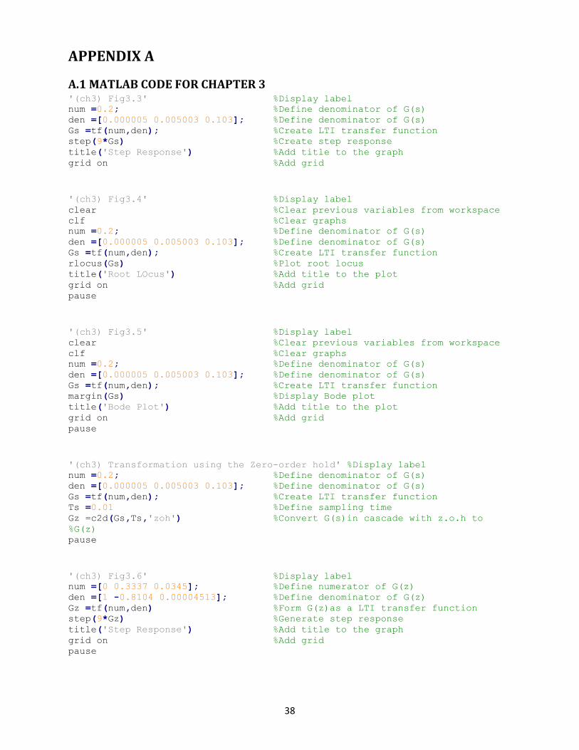
A.1 MATLAB CODE FOR CHAPTER 3 '(ch3) Fig3.3' %Display label
num =0.2; %Define denominator of G(s)
den =[0.000005 0.005003 0.103]; %Define denominator of G(s)
Gs =tf(num,den); %Create LTI transfer function
step(9*Gs) %Create step response
title('Step Response') %Add title to the graph
grid on %Add grid
'(ch3) Fig3.4' %Display label
clear %Clear previous variables from workspace
clf %Clear graphs
num =0.2; %Define denominator of G(s)
den =[0.000005 0.005003 0.103]; %Define denominator of G(s)
Gs =tf(num,den); %Create LTI transfer function
rlocus(Gs) %Plot root locus
title('Root LOcus') %Add title to the plot
grid on %Add grid
pause
'(ch3) Fig3.5' %Display label
clear %Clear previous variables from workspace
clf %Clear graphs
num =0.2; %Define denominator of G(s)
den =[0.000005 0.005003 0.103]; %Define denominator of G(s)
Gs =tf(num,den); %Create LTI transfer function
margin(Gs) %Display Bode plot
title('Bode Plot') %Add title to the plot
grid on %Add grid
pause
'(ch3) Transformation using the Zero-order hold' %Display label
num =0.2; %Define denominator of G(s)
den =[0.000005 0.005003 0.103]; %Define denominator of G(s)
Gs =tf(num,den); %Create LTI transfer function
Ts =0.01 %Define sampling time
Gz =c2d(Gs,Ts,'zoh') %Convert G(s)in cascade with z.o.h to
%G(z)
pause
'(ch3) Fig3.6' %Display label
num =[0 0.3337 0.0345]; %Define numerator of G(z)
den =[1 -0.8104 0.00004513]; %Define denominator of G(z)
Gz =tf(num,den) %Form G(z)as a LTI transfer function
step(9*Gz) %Generate step response
title('Step Response') %Add title to the graph
grid on %Add grid
pause
39
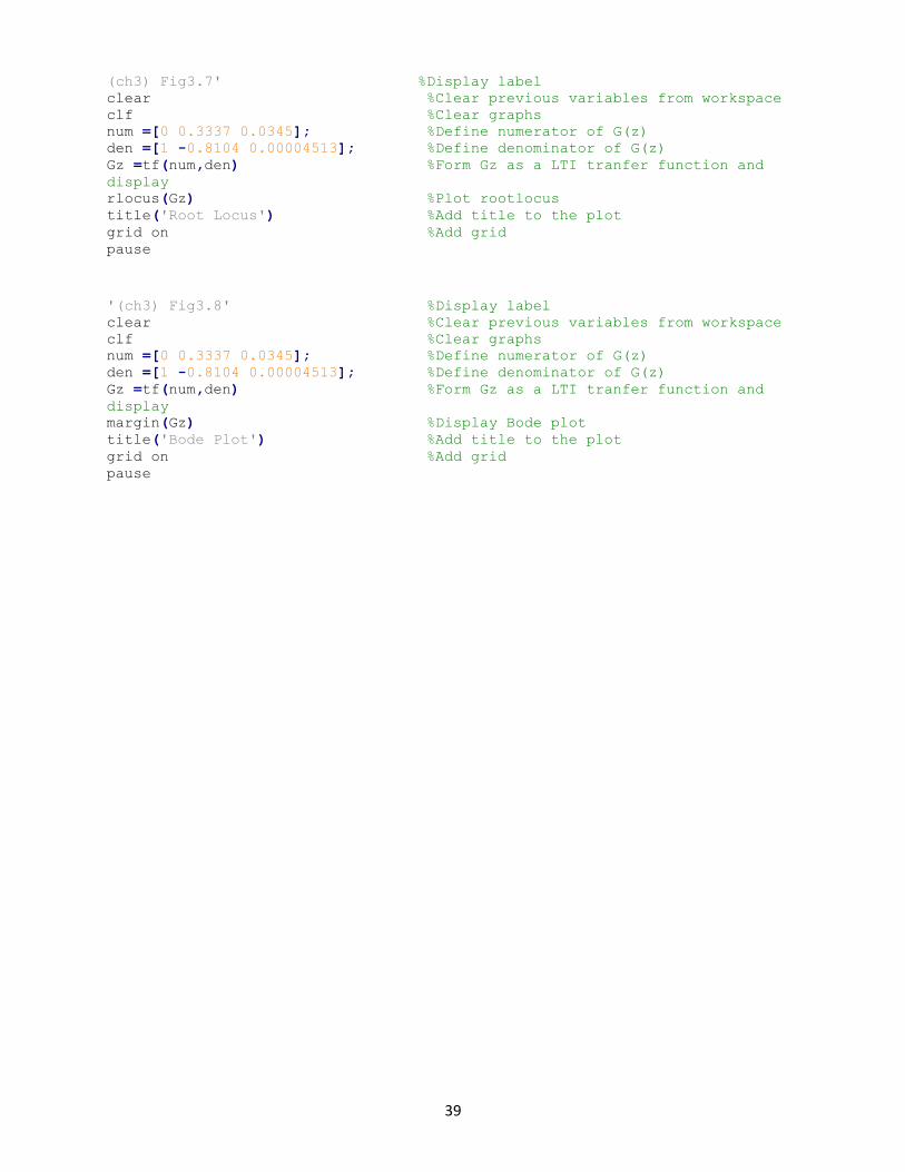
(ch3) Fig3.7' %Display label
clear %Clear previous variables from workspace
clf %Clear graphs
num =[0 0.3337 0.0345]; %Define numerator of G(z)
den =[1 -0.8104 0.00004513]; %Define denominator of G(z)
Gz =tf(num,den) %Form Gz as a LTI tranfer function and
display
rlocus(Gz) %Plot rootlocus
title('Root Locus') %Add title to the plot
grid on %Add grid
pause
'(ch3) Fig3.8' %Display label
clear %Clear previous variables from workspace
clf %Clear graphs
num =[0 0.3337 0.0345]; %Define numerator of G(z)
den =[1 -0.8104 0.00004513]; %Define denominator of G(z)
Gz =tf(num,den) %Form Gz as a LTI tranfer function and
display
margin(Gz) %Display Bode plot
title('Bode Plot') %Add title to the plot
grid on %Add grid
pause
40
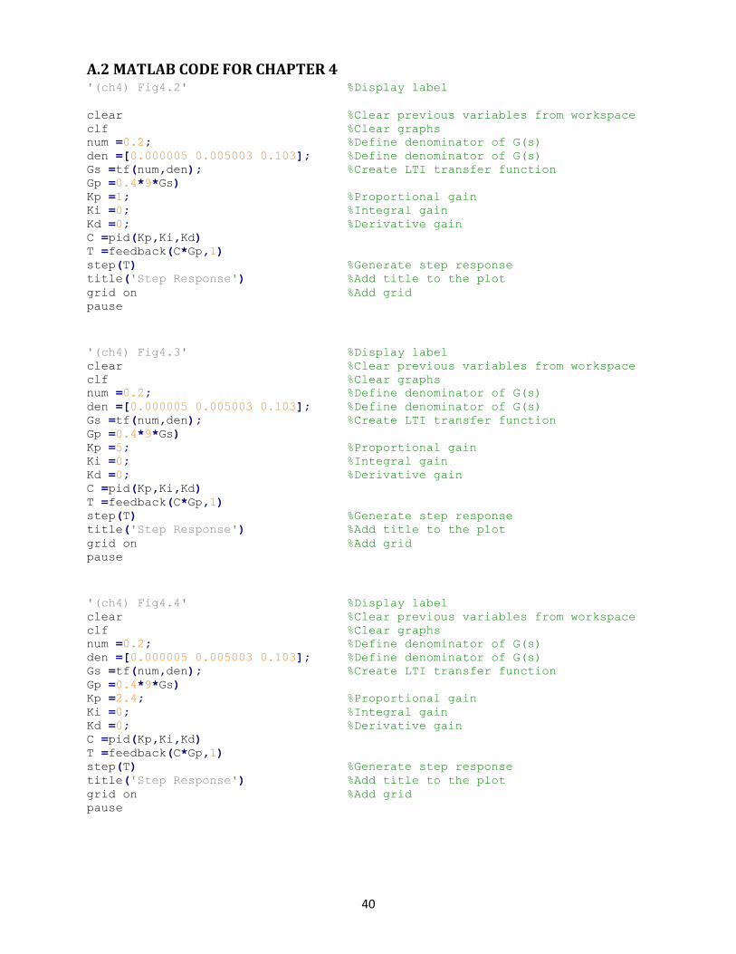
A.2 MATLAB CODE FOR CHAPTER 4 '(ch4) Fig4.2' %Display label
clear %Clear previous variables from workspace
clf %Clear graphs
num =0.2; %Define denominator of G(s)
den =[0.000005 0.005003 0.103]; %Define denominator of G(s)
Gs =tf(num,den); %Create LTI transfer function
Gp =0.4*9*Gs)
Kp =1; %Proportional gain
Ki =0; %Integral gain
Kd =0; %Derivative gain
C =pid(Kp,Ki,Kd)
T =feedback(C*Gp,1)
step(T) %Generate step response
title('Step Response') %Add title to the plot
grid on %Add grid
pause
'(ch4) Fig4.3' %Display label
clear %Clear previous variables from workspace
clf %Clear graphs
num =0.2; %Define denominator of G(s)
den =[0.000005 0.005003 0.103]; %Define denominator of G(s)
Gs =tf(num,den); %Create LTI transfer function
Gp =0.4*9*Gs)
Kp =5; %Proportional gain
Ki =0; %Integral gain
Kd =0; %Derivative gain
C =pid(Kp,Ki,Kd)
T =feedback(C*Gp,1)
step(T) %Generate step response
title('Step Response') %Add title to the plot
grid on %Add grid
pause
'(ch4) Fig4.4' %Display label
clear %Clear previous variables from workspace
clf %Clear graphs
num =0.2; %Define denominator of G(s)
den =[0.000005 0.005003 0.103]; %Define denominator of G(s)
Gs =tf(num,den); %Create LTI transfer function
Gp =0.4*9*Gs)
Kp =2.4; %Proportional gain
Ki =0; %Integral gain
Kd =0; %Derivative gain
C =pid(Kp,Ki,Kd)
T =feedback(C*Gp,1)
step(T) %Generate step response
title('Step Response') %Add title to the plot
grid on %Add grid
pause
41
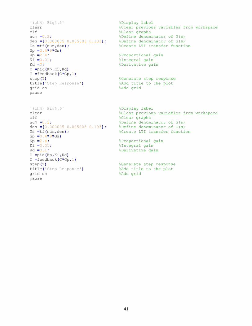
'(ch4) Fig4.5' %Display label
clear %Clear previous variables from workspace
clf %Clear graphs
num =0.2; %Define denominator of G(s)
den =[0.000005 0.005003 0.103]; %Define denominator of G(s)
Gs =tf(num,den); %Create LTI transfer function
Gp =0.4*9*Gs)
Kp =2.4; %Proportional gain
Ki =0.01; %Integral gain
Kd =0; %Derivative gain
C =pid(Kp,Ki,Kd)
T =feedback(C*Gp,1)
step(T) %Generate step response
title('Step Response') %Add title to the plot
grid on %Add grid
pause
'(ch4) Fig4.6' %Display label
clear %Clear previous variables from workspace
clf %Clear graphs
num =0.2; %Define denominator of G(s)
den =[0.000005 0.005003 0.103]; %Define denominator of G(s)
Gs =tf(num,den); %Create LTI transfer function
Gp =0.4*9*Gs)
Kp =2.4; %Proportional gain
Ki =0.01; %Integral gain
Kd =0.1; %Derivative gain
C =pid(Kp,Ki,Kd)
T =feedback(C*Gp,1)
step(T) %Generate step response
title('Step Response') %Add title to the plot
grid on %Add grid
pause
42
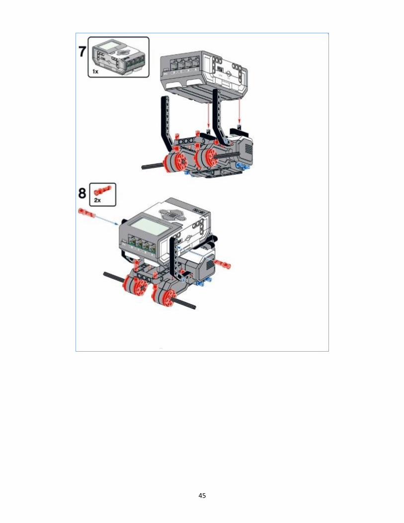
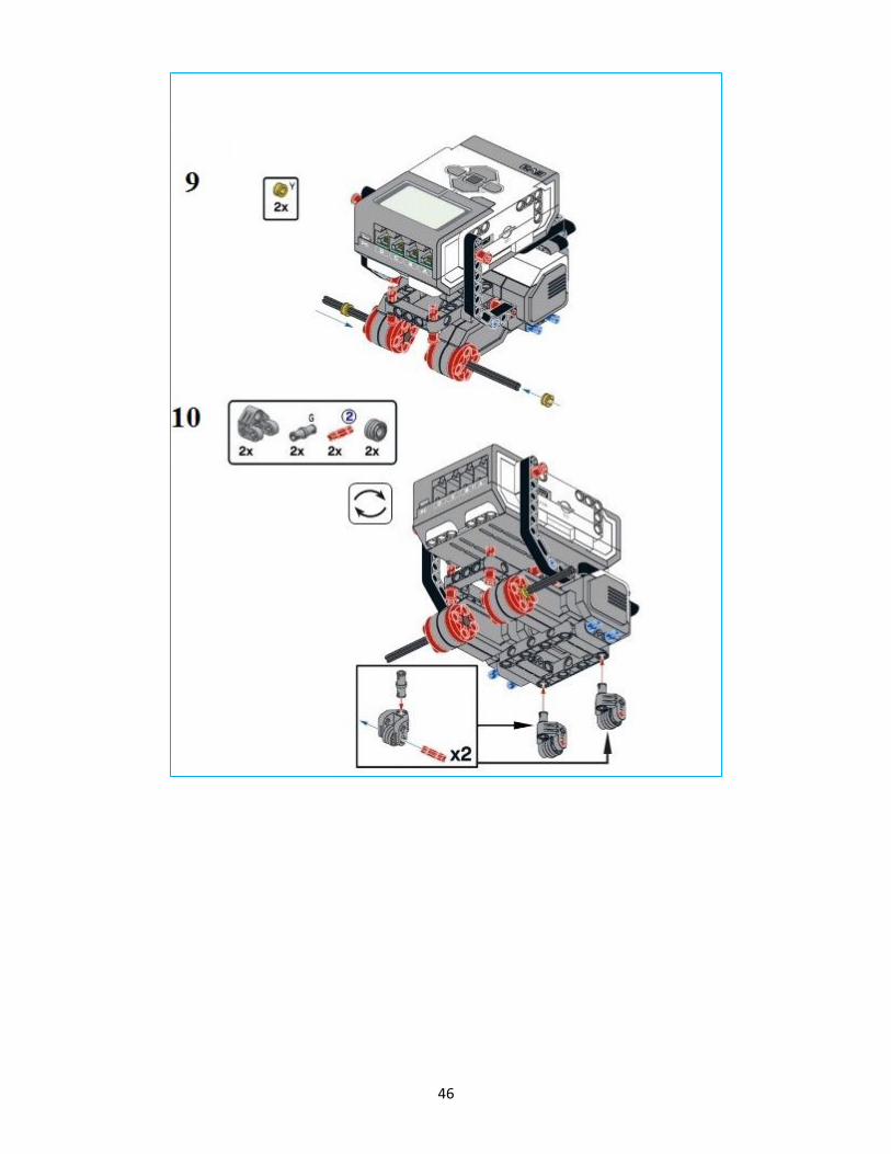
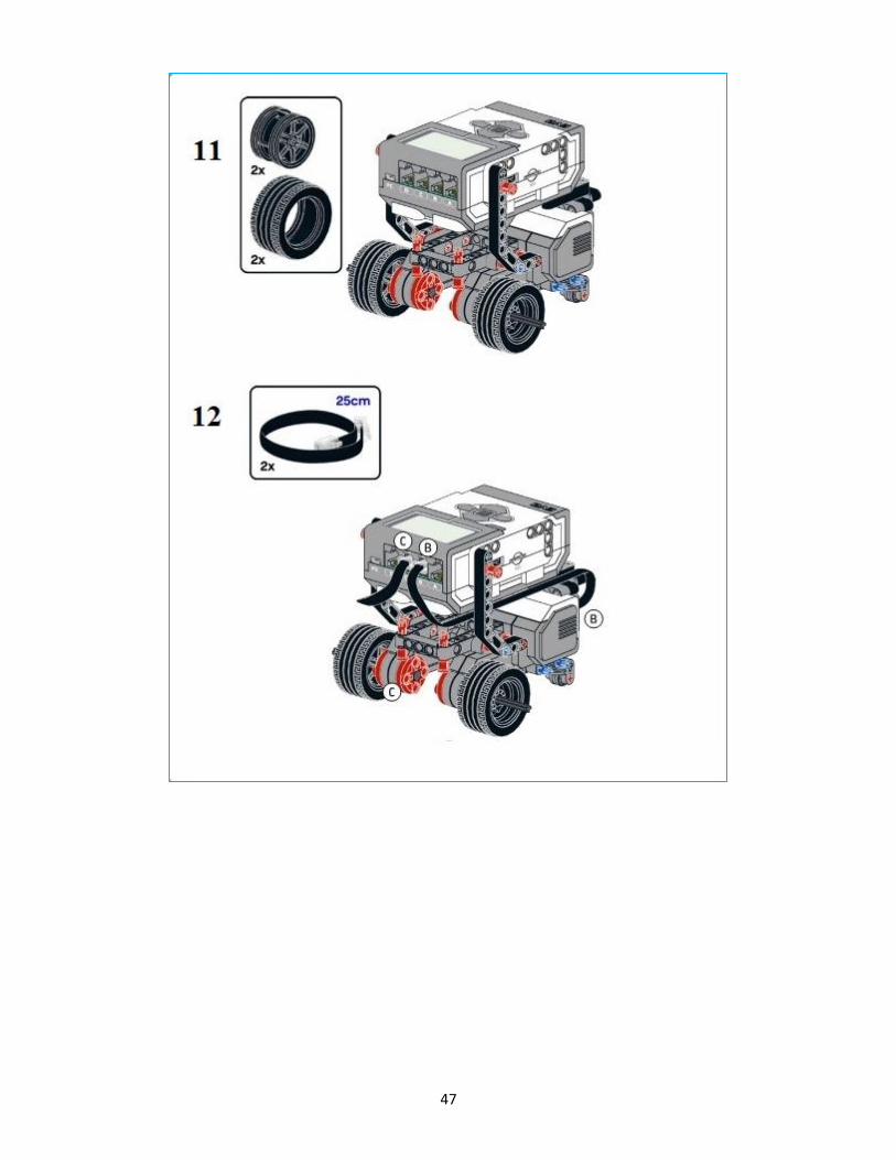
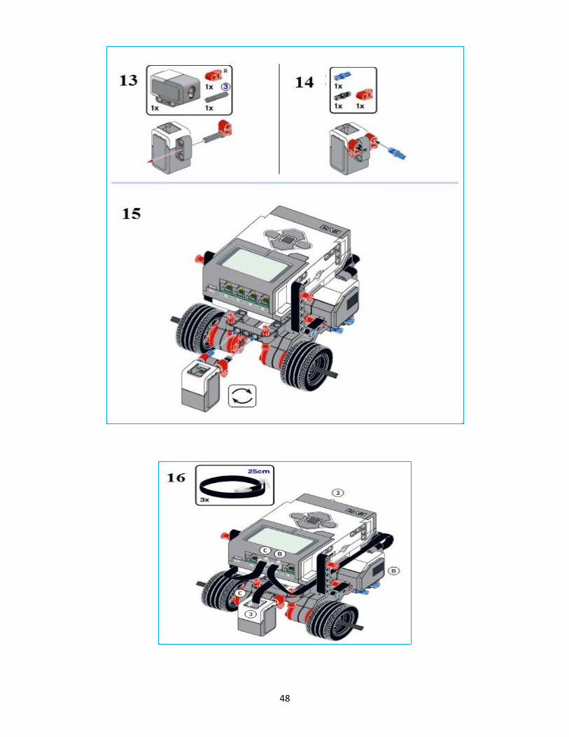
APPENDIX B: BUILDING THE LINE FOLLOWING ROBOT
43
44
45
46
47
48