Progress Report for Contract

NAS8-98203

Auroral, Polar Cap, and Polar Cusp Modeling and Data Analysis for the IMAGE Missionand LENA Instrument

Prepared for:

National Aeronautics and Space Administration

George C. Marshall Space Flight Center

Prepared by:

Gordon R. Wilson

Mission Research Corporation

One Tara Blvd., Suite 302

Nashua, NH 03062

October, 2001

https://ntrs.nasa.gov/search.jsp?R=20010108000 2018-05-05T21:09:53+00:00Z

1. Description of Progress

A) LENA Work

One of the chief mysteries in the LENA perigee pass data is the lack of an apparent auroral

oval in the images. Another is that in some cases ENA are seen from any direction near the

Earth regardless of the latitude of the spacecraft. These facts lead one to ask a fundamental

question: Is the instrument responding to ENA primarily? One possible way to get out of the

'ambiguity' of the data is to assume that at least part of the signal is produce by something other

than ENA. The two main candidates for this "something else' are UV light and energetic

charged particles.

UV light could only effect the instrument when its fan shaped aperture points toward the

source. The most intense of which will be the sun, with day glow being the second strongest and

the auroral zone, the third. We can rule out UV light as a prime source of counts in the perigee

pass data for the following reasons. 1) The perigee pass signal is different in form and much

stronger than the sun pulse signal seen just before or just after perigee. 2) There is no indication

of the auroral zone, which would produce at least two peaks in the counts versus spin phase

curve. 3) Mike Colliers' analysis of the sun pulse signal shows that it varies with the flux of thesolar wind and not with variations in the solar UV flux.

Charge particles that enter the aperture of the instrument and produce counts would show up

when the instrument looks in the direction from which they come. In all of the data I am

analyzing voltages were being applied to the collimators so that most charged particles should

have been excluded from the instrument but this effect could still show up where the flux of

energetic particles is high enough. The most likely place would be in the auroral zone where

energetic electrons and protons precipitate. If these particles are producing counts then they

should be seen when the instrument looks in and near the zenith direction. In nearly all of the

perigee passes the zenith direction is devoid of counts.

The relationship between LENA perigee flux intensities and measures of magnetic and

solar activity, and instrument state

Over the last two months I have finished processing all of the useable perigee pass data

between the dates of 10 June and 29 August 2000. The data set consists of 99 perigee passes. I

have prepared blow up spectrograms of each pass correcting the data by removing backgroundcounts.

The first thing shown here is a plot for the three-month interval that nicely summarizes many

of the issues found in this analysis. Figure I is a plot of the Ap history for the three-month

interval of June, July and August 2000. Over plotted in each month's panel is the total count

intensity for each perigee pass. This quantity is found by summing all of the valid H and O

counts (background subtracted) for the 10 to 18 images bracketing each pass.

The passes displayed in figure 1 can be divided into one of three groups. The first group

consists of passes whose variation in total intensity tracks well the variation in magnetic activity.

This set consists of perigee passes from June 10th to June 28 th and July 26 th to July 30 th. The

second group consists of the passes between 29 June and 9 July 2000 and is characterized by an

almost complete lack of correlation with magnetic activity. The variations seen in the total

intensity for this set suggests that the instrument was switching between two different operatingstates almost from one orbit to the next. There is however no evidence in the state tables for the

dates in question to show that that was the case.

The last group of passes consists of those that occurred between 31 July and 29 August 2000.

Here again there js a lack of correlation between total intensity and magnetic activity but in

addition,thetotal intensityof eachpassis onaveragelargerthantheothertwo groups•Thefirst

perigee_passin this groupoccurrednear0920UT on the 31st of July and had a total intensity ofover 10 counts, the most intense of the entire data set. The behavior during the first three days

of this set suggests that the instrument was made very sensitive on the 31 st and that over the next

two days the gain was turned down. (There is a significant up swing in magnetic activity on the

31 st to a Kp of 5+ but this occurs after the perigee pass.) There were a large number of changes

made in the state of the instrument on the 31 st prior to the perigee pass on that date.

Below is a table that summarizes the state of the instrument for the three perigee pass groups

described above. As far as I can tell there was no change in how the instrument was operated

between the 10 June and 30 July 2000. Nearly all instrument settings were maintained constant

during this interval with the exception of the stop MCP voltage which was turned down during

outbound radiation belt passage. The voltage reduction occurred in a single step usually prior to

the spacecraft reaching perigee. This instrument state change is reflected in the data by reduced

image intensity and a drop in the O/H ratio. Since there was apparently no change in the way the

instrument was operated between perigee pass group 1 and 2 the odd behavior of the data

between June 29 th and July 9 th is still a mystery.

There appears to be hope in explaining why the data from the August perigee passes differs

so much from the June and July passes. For one thing the collimator voltages were higher (96

versus 86), the optics HVPS was enabled and set to 128 and flight software version 1 replaced

version 24. Another difference was the way radiation belt passages were handled in August

versus the earlier months. For one thing the minimum value was higher (131 versus 128) and it

varied over the course of the month. For example, between August 2 nd and August 19th the

minimum was 131 to 132 but after August 19 th it ranged between 138 and 139. There is a

noticeable increase in the overall intensity of the perigee passes starting on August 20 th. For the

bright perigee passes of July 31 st and August 1st the minimum value of the stop MCP voltage was

138. Another difference between the June-July and August perigee passes is that the stop

voltage reductions were often done in several steps rather than one. In many cases there would

be 4 to 5 steps spread over about 30 minutes.

PerigeePass

Group

Dates Start Stop Coil Coll Optics Steer. Start Stop FSW

MCP MCP Pos Neg CFD CFD Ver.

June10-28 144 128/144 86 86 disabled 0 2 6 24

July 10-30June 29- 144 128/144 86 86 disabled 0 2 6 24

July 9

July 31- 144 131-144 96 96 128 0 2 6 1

Aug. 29

One way to test the hypothesis that the fluxes seen by LENA during perigee passes are

produced by upflowing ions is to see how well the fluxes correlate with magnetic activity. To• th 2 th 2000that end I have taken the total counts from 50 perigee pass from the June 10 to July 9

time interval (groups 1 and 2) and plotted them versus the concurrent value of Ap. (see figure 2)

The correlation coefficient for this data set is 0.55, which is good but not fantastic.

The emission of ENA from the auroral and high latitude ionosphere depends on the flux of

energetic ions (O + or H +) and on the column abundance of atomic oxygen above the ion heating

region. It is well know that the flux of energetic ions varies with magnetic and auroral zone

activity. The column abundance of O in the high latitude thermosphere also varies with

magneticactivity but on longertime scales.For example,for theMSIS86model to calculateanaltitudeprofile of atomicoxygenonecaninput magneticactivity informationfor up to three days

prior to the time of interest. It is also know from general circulation modeling results that when

the high latitude ionosphere is stirred by the electric field imposed on the magnetosphere by the

solar wind the neutral thermosphere is stirred as well. This leads to low densities on the dawn

and dusk sides of the polar cap and high densities in the cusp and midnight auroral zone regions.

Off times higher densities extend across the polar cap in the noon-midnight direction. This

means that all else being equal, the cusp and midnight auroral zone regions should be more

prolific producers of ENA than the dusk and dawn auroral zones.

" f'i !80 June 2000

6o n

/ '_ / tl

II" _jI I _ _ tt2O _ • _ -o

5 10 15 20 _ 30

'!I'"'°_0 _I _II I'

5 10

I

(

i

J

• i

15

I

f_

/

I_I

I

I-

3o

loo

_o

6o

o • ,,_ ILa_.-'E.'' .-- , . -

5 lO 15 20 25 30Day _ 1_N_nlh

Figure 1. Ap history for the summer of 2000. Over plotted in each panel (filled squares) is the

total intensity of the LENA counts in each perigee pass divided by 1000.

8.10 4 .... I .... I ....

Figure 2.

pass.

6.1o4

c

4-104

" L !2.104 H "

• []

0 , , , I .... I , , , ,

0 50 100 150

Ap

Plot of the total counts in each perigee pass versus the Ap index for the time of the

Variations in the column abundance among these regions can be up to a factor of 5. Given

that these conditions take longer to set up (then increases in the ion heating rate) and persist for a

while after magnetic activity subsides it is reasonable to expect that ENA emissions might

correlate also with magnetic activity from the resent past. To that end I test the 50 passes used in

figure 2 with the Ap index from the previous four Ap intervals and got correlation coefficients of

Ap History

Current Ap

Correlation Coefficient

Group 10.61

Correlation Coefficient

Groups 1 + 20.55

0.34Ap (-1) 0.39

Ap (-2) 0.39 0.34

Ap (-3) 0.06 0.08

Ap (-4) 0.19 0.200.56 0.49

0.67(-1)

(-2) 0.57

0.45

Current Ap + Ap

Current Ap + Ap

Current Ap + Ap

Current Ap + Ap

Current Ap + Ap

Current Ap + Ap

(-3) 0.51

(-4) 0.56 0.490.59 0.51

0.53

0.45Current Ap + Ap

(-1) + Ap (-2)

(-2) + Ap (-3)

(-3) + Ap (-4)

0.46

0.40

0.34, 0.34, 0.08, 0.2 respectively. Clearly the perigee pass intensities correlate better with

current activity than with past activity.

To get large perigee fluxes from heated ionospheric ions requires high heating rates at the

time of the perigee pass as well as high O densities. This suggests that some combination of

current and past magnetic activity may be required for maximum emissions. To that end I havecalculated the correlation coefficient for the following cases listed in the following table. Here I

use two data groups, those from perigee pass group 1 and those from group 1 and 2. This is done

to see the effect that group 2 has on the correlations.

The highest correlation coefficient is for the case that uses the current Ap and the one from

two Ap intervals back. The difference however is only a marginal improvement for the

combined groups but is somewhat significant for group 1 alone.

C

O

cjg.

8.I04

6.104

4-104

|vi,111

[]

'il,

Hi n nun

• liiil2-10 4D • []

[" "1- "

0 50 100 150

Ap + Ap(-2)

Figure 3. Plot of the total counts in each perigee pass in group 1 versus the Ap index for the

time of the pass plus the Ap index from 6 hours past. This is the condition with the maximum

correlation.

Because of the well know correlation between the flux of escaping suprathermal O+ ions and

the level of solar activity I show in figure 4 below a plot similar to figure 1 except that Ap has

been replaced with Fl0.7. There seems to be little relationship between the perigee pass sum

counts and solar activity. Note the overall decline in the sum counts between July 3 and July 9

when F10.7 is increasing. Note also the interval from August 15th to the 25 tla when F]0.7 is

decreasing but sum counts is increasing.

41 _ , .... i

3OD

June 2000

JI- [] ,, •_- -- I 1 IL

'°°V ,,,, •..•n= W L'' ='_

Ii I - --I - i0

5 10 15 20 _ 30

._CCl _ . , i ,

July 2000Iz

300 _-] r-i]E ,

,,,'°°L-,,,. _,_, "r.'-, ------_, "..=. a

FI I i I '-I i -- ',,,- ,' -4oFI I ,=,i..-I , .... , .... , , ._ • ,'_5 I0 15 20 _ 30

5 10 15 20 _ 30

Da 7 c_ _ni.h

Figure 4. F10.7 history for the summer of 2000. Over plotted in each panel (filled squares) is the

total intensity of the LENA counts in each perigee pass divided by 300.

Individual Examples

Figure 5 below shows my typical blow up plot of the perigee data from July 31, 2000. In

addition to the lines showing the trailing limb, nadir, approaching limb and ram directions, there

is a series of diamonds showing the track of the sun's direction across the field of view. This

perigee pass had the highest sum count total (>105) of any pass in the June-August 2000 interval.

Theinterestingthing aboutthis passis how thestopMCPvoltagevariedduring the interval.Accordingto thestatelogsthis voltagewassetat 144up until 0917:01whenit was reducedto138. It wasincreasedto 143at 0923:01and144at 0927:00.So,for themostpart the instrumentretaineda high sensitivitytroughout thepassandinto theradiationbelts. Thereis a slight dropin the O/H ratio between0912and0917UT which couldbe dueto the slight reductionin thestopMCPvoltagealthoughthetiming doesn'tquite lineupwith thevaluesfrom thestatetable.

5

10

01

July 31, 2000 (DOY 213)

Counts

100

35 10

4O

10.0

O

t._. 1.0

0.1 I ' ' I ' ' I '9:05:55 9:11:55 9:17:55

2983 1982 1310-58 -77 -78

4:04 4:16 15:39

' I ' ' I '9:23:54 9:29:56

1316 1938-53 -29

15:51 15:55

UT

Alt (kin)MLat

MLT

Figure 5. Perigee pass data for July 31, 2000.

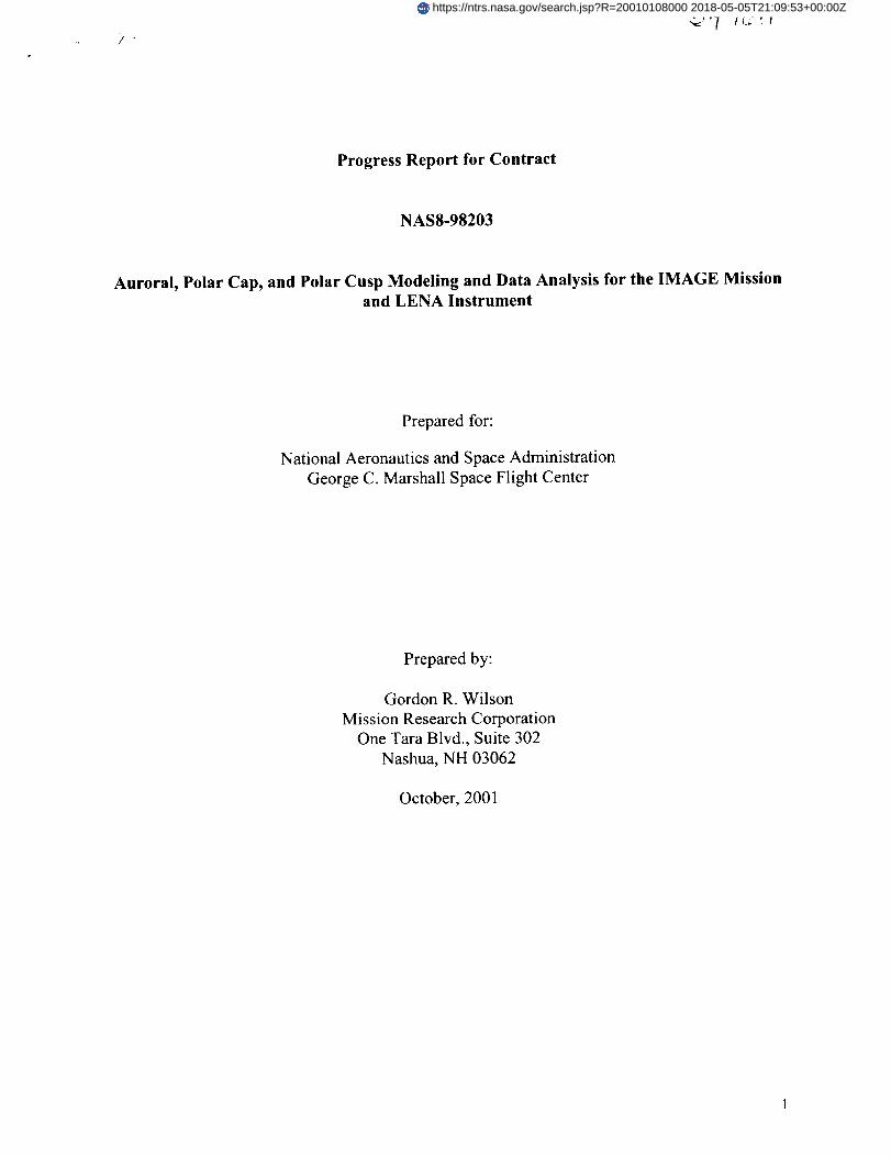
Because of the different way in which the stop MCP voltage was varied during this perigee

pass compared to previous passes, this case is likely the clearest example of how the low-

altitude, low-energy ENA emissions look, unencumbered by instrument effects. When compared

with my previous simulation results one can see that there is no apparent auroral oval. ENA

emissions are seen coming from the Earth regardless of whether the spacecraft is over the polar

cap, auroral zone, or low latitudes. There is an overall shift in the direction of peak emissions

from the nadir direction to the approaching limb/ram direction.

The intensity of the images in this pass were collectively the most intense images seen on any

other perigee pass I have looked at but there was nothing particularly interesting happening that

0

5

10

30

35

4O

June 25, 2000 (DOY 177)

Counts

100 ¸

10

I0.0

0°_

L_

m5

1.0

0.1I

I I ' I ' ' ' ' I ' ' I19:08:56 19:14:58 19:20:58 19:26:57 19:32:57 UT

3358 2201 1403 1194 1635 AIt (kin)-70 -80 -64 -39 - 15 MEat

8:38 13:03 17:22 18:13 18:35 MET

Figure 6. Perigee pass from June 25, 2000. Note the missing image between 1918:58 and

1920:58. At the time of this pass Kp was 2- (Ap = 6).

day. At the time of thepassKp was2 whereit hadbeen3+ in thethree-hourtime interval (6-9UT) before. Quick look AE wasabout300nT at thetime. TheFI0.7 index was 152 for July 31,

which makes this day one of the quietist, in terms of solar activity, in the June-August time

period. Between 0000 and 1000 UT on the 31 st the solar wind density was between 4 and 7 cm -3

and the solar wind speed was between 400 and 450 km/s. The magnitude of the IMF remained

less than about 8 nT but it turned and remained southward during the three hours before the

IMAGE perigee pass. Could it be that these intense emissions are a result of a constant stirring

of the magnetosphere for 3 or more hours?

O|

5

10

15

__'20f/l

C

"_. 25

30

35

June 26, 2000 (DOY 178)

Counts

100

10

4O

10.0

Oo_

1.0

0.1 I ' ' I ' i I ' ' I ' ' I9:23:55 9:29:57 9:35:57 9:4l:56 9:47:56 UT

3177 2004 1308 1220 1764 Alt (km)-60 -79 -76 -50 -26 MLat

5:38 4:36 19:22 18:33 18:20 MLT

Figure 7. 1st Perigee pass from June 26, 2000. Kp at the time of this pass was 5 (Ap - 48).

10

Below I show a few additional examples to illustrate the trends discussed above. The first

two are perigee passes from June 25 thand 26 th (see figures 6 and 7). The main thing to note in

this pair of consecutive passes is the change in the overall intensity of the images from a value of3088 total counts for June 25 th to 72660 total counts for June 26 th. Between the times of these

two passes Kp changed from 2- to 5. Also visible in this data is when the stop voltage reduction

took effect. From the instrument state tables the reduction during the June 25 th pass occurred at

1920:56 UT and for the June 26 th pass it occurred at 0937:55 UT.

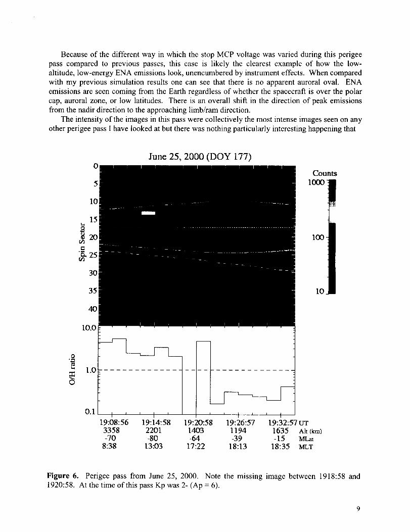
The next pair of example passes comes from July 2, 2000 and are part of group 2. The total

number of counts for the first of these passes was 38847 and for the second was 5078. The value

of Kp was 1 for both of these passes. In terms of magnetic activity July 2 ndwas a very quite day

where Kp never got above 2-. The stop MCP voltage was redticed to 128 twice on the 2 nd at0757:40 and 2206:39 UT.

O|

10

30

35

July 2, 2000 (DOY 184)

Counts

I00

I0

10.0

O

1.0 ................

0.1 I _ ' I I ' _ ' I

7:43:40 7:49:42 7:55:42 8:01:41 8:07:413055 1941 1319 1286 1864-63 -79 -72 -47 -23

4:54 2:46 19:22 18:23 18:04

UT

Alt (km)MLatMLT

Figure 8. First perigee pass from July 2, 2000. Kp for this pass was 1 (Ap = 4).

11

0|

5

10

30

35

40

July 2, 2000 (DOY 184)

Counts

I00 ¸

I0

10.0

O

0.1I ' ' I ' ' I ' ' I ' ' t

21:54:38 22:00:40 22:06:41 22:12:41 22:18:40 UT3669 2430 1538 1209 1491 Alt (kin)-73 -87 -67 -42 -16 ML,at

7:03 13:ll 17:53 18:12 18:18 MLT

Figure 9. Second perigee pass from July 2, 2000. Kp for this pass was 1 (Ap -- 4).

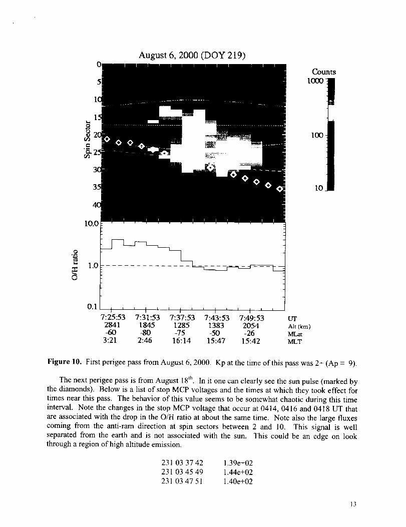
Finally I show a few examples of perigee passes from the August group whose behavior is

significantly different from the passes of June and July. The first is shown in figure 10 and is the

first pass from August 6 th. The count total for this pass was 47584. Note the gradual reduction

in the intensity of the images and the gradual reduction in the O/H ratio between the times 0734

and 0742 UT. According to the state table for this date the stop MCP voltage was 144 at the start

of the pass and was reduced to 136 at 0735:52 UT, 135 at 0737:52 UT, and 134 at 0739:51 UT.

The behavior seen in this pass seems to be consistent with what was seen earlier but spread out

due to the stepwise reduction in the stop MCP voltage.

12

O!

5

August 6, 2000 (DOY 219)

Counts

100

10

10.0

Q

5

0.1I ' i I ' i I i , I ' i I i i

7:25:53 7:31:53 7:37:53 7:43:53 7:49:53 trr

2841 1845 1285 1383 2054 Alt (kin)-60 -80 -75 -50 -26 MEat

3:21 2:46 16:14 15:47 15:42 MLT

Figure 10. First perigee pass from August 6, 2000. Kp at the time of this pass was 2+ (Ap = 9).

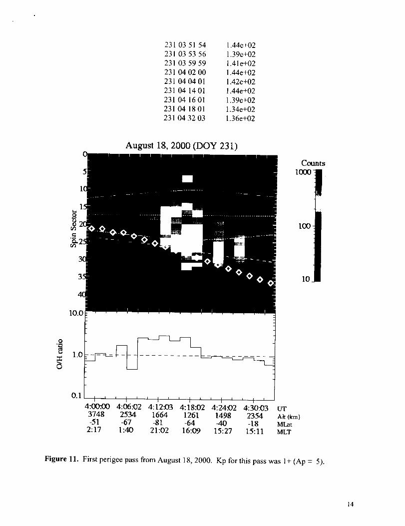
The next perigee pass is from August 18 th. In it one can clearly see the sun pulse (marked by

the diamonds). Below is a list of stop MCP voltages and the times at which they took effect for

times near this pass. The behavior of this value seems to be somewhat chaotic during this time

interval. Note the changes in the stop MCP voltage that occur at 0414, 0416 and 0418 UT that

are associated with the drop in the O/H ratio at about the same time. Note also the large fluxes

coming from the anti-ram direction at spin sectors between 2 and 10. This signal is well

separated from the earth and is not associated with the sun. This could be an edge on look

through a region of high altitude emission.

231 03 37 42 1.39e+02

231 03 45 49 1.44e+02

231 03 47 51 1.40e+02

13

231 03 51 54

231 03 53 56

231 03 59 59

231 04 02 00

231 04 04 01

231 04 14 01

231 04 16 01

231 04 18 01

231 04 32 03

1.44e+02

1.39e+02

1.41 e+02

1.44e+02

1.42e+02

1.44e+02

1.39e+02

1.34e+02

1.36e+02

August 18, 2000 (DOY 231)

Counts

100

10

I0.0

I i i I

4:00:00 4:06:02 4:12:03 4:18:02 4:24:02 4:30:03 UT

3748 2534 1664 1261 1498 2354 Alt(km)-51 -67 -81 -64 -40 -18 MLat

2:17 1:40 21:02 16:09 15:27 15:11 MLT

Figure 11. First perigee pass from August 18, 2000. Kp for this pass was 1+ (Ap = 5).

14

August20,2000(DOY 233)

Counts

100

10

0

g-d

10.0

1.0 ........

0.1 I

12:58:57 13:04:58 13:10:58 13:16:57 13:22:58 13:28:59 UT3068 1986 1353 1327 1925 2953 Alt (k:m)-62 -77 -69 -45 -22 -3 MLat

4:08 6:38 12:37 13:57 14:25 14:41 MLT

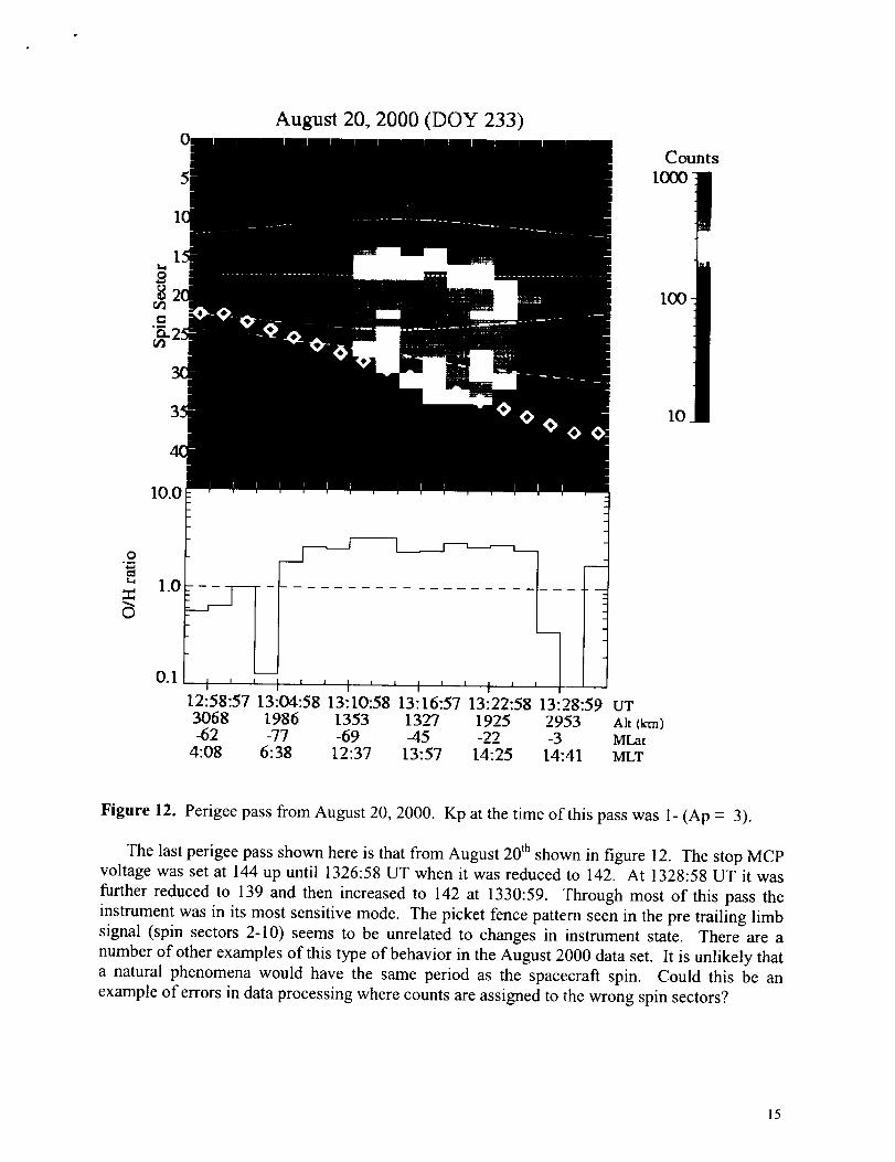
Figure 12. Perigee pass from August 20, 2000. Kp at the time of this pass was I- (Ap = 3).

The last perigee pass shown here is that from August 20 th shown in figure 12. The stop MCP

voltage was set at 144 up until 1326:58 UT when it was reduced to 142. At 1328:58 UT it was

further reduced to 139 and then increased to 142 at 1330:59. Through most of this pass the

instrument was in its most sensitive mode. The picket fence pattern seen in the pre trailing limb

signal (spin sectors 2-10) seems to be unrelated to changes in instrument state. There are a

number of other examples of this type of behavior in the August 2000 data set. It is unlikely that

a natural phenomena would have the same period as the spacecraft spin. Could this be an

example of errors in data processing where counts are assigned to the wrong spin sectors?

15

B) Description of Progress on the Plasmasphere model.

Nothing new to report.

2. Current Problems.

There are no problems affecting the continuation of this project.

3. Work to be performed during the next quarterly reporting period.

After consultations with other team members I will proceed with plans for a paper.

Cost information.

The current contract value (options 0, 1, 2, and 3) is $197182 with an end date of 31 Jan 2002.

(a) Total cumulative costs as of report date: $133409

(b) Estimated cost to complete contract: $63773

(c) Estimated percentage of completion of contract: 68%

(d) We are on tract to finish this portion of the overall project.

This project has been modified and divided into two subtasks. Subtask 01 covers the LENA

The numbers

.

instrument support work and subtask 02 is the plasmasphere-modeling project.

above cover the total contract (subtasks 01 and 02).

16