Final Report - NASA · · 2013-08-30Final Report Contract No. NAS8-38348 ... analyses with reduced order models developed from a SPARfEAL finite element model ... computational

# - v'_

- ..,// _,_,

Final Report

Contract No. NAS8-38348

George C. Marshall Space Flight CenterNational Aeronautics and Space Administration

Marshall Space Flight Center, AL 35812

J. H. Griffin and M-T. Yang

Department of Mechanical Engineering

Carnegie Mellon University

Pittsburgh, PA 15213(NASA-CR - /_L._w_ MODELING THE

EFFECI OF SHROUD CONTACT AND

FRICTION DAMPFRS ON THE MISTUNED

RESPONSE OF TURBOPUMPS Final

_eport, 31 May 1991 - 31 Aug. 199_(Carnegie-Mellon Univ.) 79 p

N95-20795

January 1994Uncl as

G3/37 0061091

https://ntrs.nasa.gov/search.jsp?R=19950014378 2018-06-22T08:39:35+00:00Z

INTRODUCTION AND BACKGROUNDI I

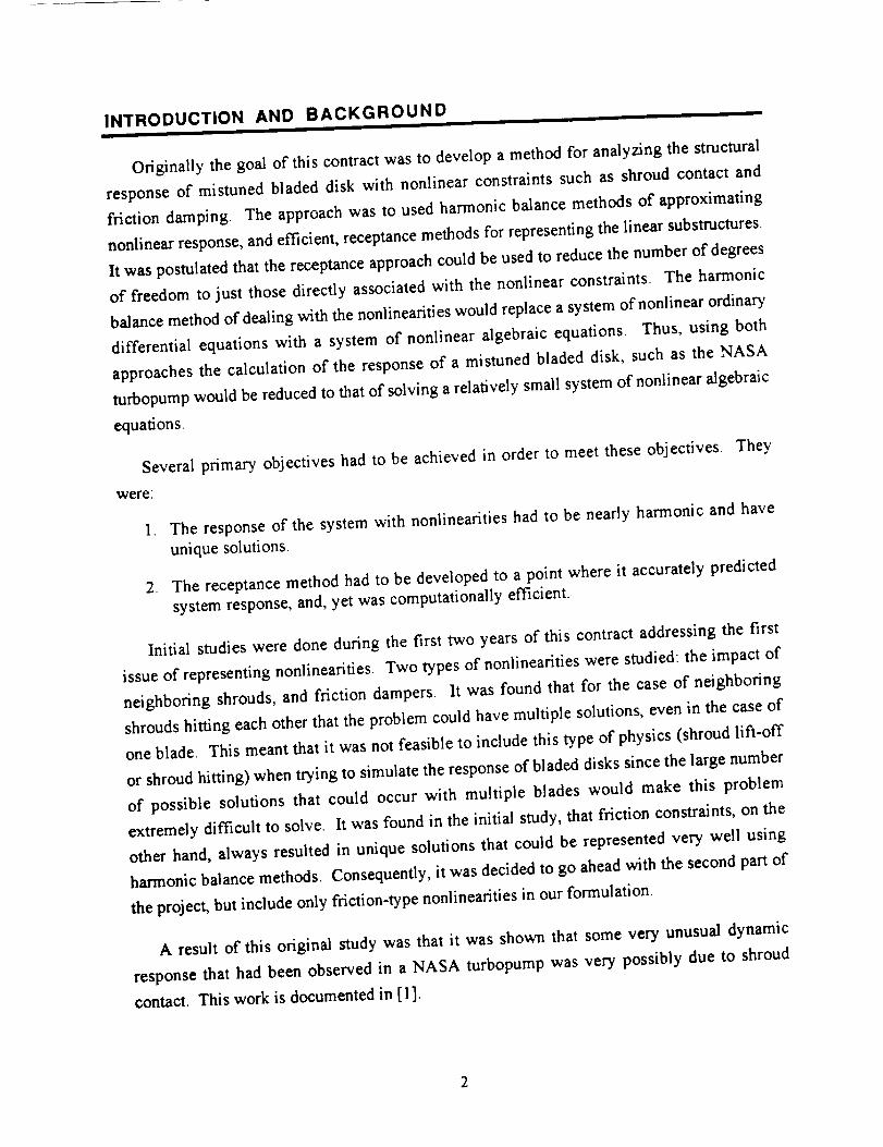
Originally the goal of this contract was to develop a method for analyzing the structural

response of mistuned bladed disk with nonlinear constraints such as shroud contact and

friction damping. The approach was to used harmonic balance methods of approximating

nonlinear response, and efficient, receptance methods for representing the linear substructures.

It was postulated that the receptance approach could be used to reduce the number of degrees

of freedom to just those directly associated with the nonlinear constraints. The harmonic

balance method of dealing with the nonlinearities would replace a system of nonlinear ordinary

differential equations with a system of nonlinear algebraic equations. Thus, using both

approaches the calculation of the response of a mistuned bladed disk, such as the NASA

turbopump would be reduced to that of solving a relatively small system of nonlinear algebraic

equations.

Several primary objectives had to be achieved in order to meet these objectives. They

were:

.

,

The response of the system with nonlinearities had to be nearly harmonic and have

unique solutions.

The receptance method had to be developed to a point where it accurately predicted

system response, and, yet was computationally efficient.

Initial studies were done during the first two years of this contract addressing the first

issue of representing nonlinearities. Two types of nonlinearities were studied: the impact of

neighboring shrouds, and friction dampers. It was found that for the case of neighboring

shrouds hitting each other that the problem could have multiple solutions, even in the case of

one blade. This meant that it was not feasible to include this type of physics (shroud lift-off

or shroud hitting) when trying to simulate the response of bladed disks since the large number

of possible solutions that could occur with multiple blades would make this problem

extremely difficult to solve. It was found in the initial study, that friction constraints, on the

other hand, always resulted in unique solutions that could be represented very well using

harmonic balance methods. Consequently, it was decided to go ahead with the second part of

the project, but include only friction-type nonlinearities in our formulation.

A result of this original study was that it was shown that some very unusual dynamic

response that had been observed in a NASA turbopump was very possibly due to shroud

contact, This work is documented in [1 ].

A formulation was then developed for reducing the number of degrees of freedom in a

mistuning analysis. Initial work had been done in developing this approach when NASA

decided that it had to significantly reduce funding for this project. As a consequence, it was

agreed that the statement of work for this contract would be revised and the deliverables

changed to the following:

Complete the development of a computer code for performing linear mistuning

analyses with reduced order models developed from a SPARfEAL finite element model

of the blade and an annular disk. Reduced order models are models that can be

explicitly derived from the finite element model and that have significantly fewer

degrees of freedom than a comparable finite element model, e.g., 10,000 degrees of

freedom per blade reduced to six.

The code will be based on a Monte Carlo type analysis in which the frequencies of the

blades vary randomly and the forced response is calculated over a range of excitation

frequencies.

• Documentlinear mistuning code

• Prepare a paper on the mistuning analysis of a NASA turbopump for the Advanced

Earth-to-Orbit Propulsion Technology -- 1994 Conference.

Consequently, the final effort on this contact has focused on developing a linear mistuning

code and that development and documentation is the focus of this report. A paper on the

mistuning analysis of a NASA turbopump is included in volume II of the Proceedings of the

Advanced Earth-to-Orbit Propulsion Technology -- 1994 Conference and is cited as

reference 2.

DEVELOPMENT

CODEi

AND DOCUMENTATION OF LINEAR MISTUNING

The development and documentation of the linear mistuning code is documented in the

three appendices of this report. They are:

* Appendix A: Summary Report. This summary report provides a brief summary of

the theory and application of the linear mistuning code.

• Appendix B: User Manual. This manual specifies the input requirements for running

the linear mistuning code.

Appendix C: Theoretical Manual. This manual provides a detailed explanation of the

theory and application of the linear mistuning code (in effect, this is an expanded

version of Appendix A).

DELIVERY OF LINEAR MISTUNING CODEI

The linear mistuning computer code (LMCC) and the input files used in analyzing the

NASA turbopump have been transferred to NASA Marshall Silicon Graphics Computer on

which the researchers where given an account. The example case, the NASA turbopump, ran

correctly on the NASA computer. There was a problem with compatibility in transferring to

the Silicon Graphics computer at NASA in that the random number generating subroutine did

not work correctly on the Silicon Graphics if certain optimization options were used during

its compilation. This problem is documented in the User Manual.

Thus, LMCC and example files have been successfully delivered to NASA Marshall at

this time.

KEY RESULTS

Interesting results from running LMCC are discussed at some length in Appendix A.

Briefly, however there are two key results:

1. It works well, i.e., it is computationally efficient and accurate.

. When the disk is stiff, it predicts very different mistuned response from the mass

spring models that were used in the past. LMCC shows that bladed disk systems

can have a large amount of amplitude scatter from blade to blade even when the

disk is very stiff The old mass/spring models predict that, in this case, the blades

would act as uncoupled, independent systems (the disk is almost a rigid

foundation) and that there would be very little amplitude scatter. This could be a

very important result if NASA decides to go to bladed disk systems with stiff

disks, e.g. if they decide to use integral bladed disks. (Experimentalists at the

engine companies have also observed large blade to blade scatter and reported that

the mass spring models did not predict this behavior,)

RECOMMENDATIONSII

Several things could be done to make the linear mistuning code more efficient, more

accurate, or more convenient. The primary ones are:

]. Modify the input data so that the disk modes could be calculated using cyclic

symmetric boundary conditions in EAL. Currently, LMCC requires that the

modes of the disk be calculated using a model of the full disk.

4

. Add aerodynamic coupling between the blades. Currently, only blade and disk

modal damping are included During a NASA review, this option was not judge to

be very important since most NASA applications correspond to very short stiff

blades.

3. Modify the input preprocessor so that LMCC is compatible with other finite

element codes Currently, it only works with EAL or SPAR programs.

Nonlinear constraints could also be added to the formulation. For example, with

appropriate modifications LMCC could handle shroud friction constraints in a very efficient

manner.

Lastly, LMCC could be a very useful tool in assessing various strategies for actively

controlling bladed disk response The reason for this is that its structural fidelity would allow

the researcher to quantitative assess the effect on system response of putting actuators at

various locations on the disk and blades.

REFERENCESI

l, J. H. Griffin, and M. T. Yang, "Exploring How Shroud Constraints Can Affect Vibratory

Response in Turbomachinery," Proceedings of the Advanced Earth-to-Orbit Propulsion

Technology Conference, 1992, pp 569-578.

, M. T. Yang, J. H. Griffin, and L. Kiefling, "Mistuned Vibration of Bladed Disk

Assemblies: A Reduced Order Approach," Proceedings of the Advanced Earth-to-Orbit

Propulsion Technology Conference, 1994, pp 451-455.

Appendix A: Summary Report

EXECUTIVE SUMMARY

A reduced order approach is introduced that can be used to predict the steady-state

response of mistuned bladed disks. This approach directly takes results from a finite

element analysis of a tuned system and, based on the assumption of rigid blade base

motion, constructs a computationally efficient mistuned model with a reduced number of

degrees of freedom. Based on a comparison of results predicted by different approaches

it is concluded that: the reduced order model displays structural fidelity comparable to

that of a finite element model of the entire bladed disk system with significantly improved

computational efficiency; and under certain circumstances both the finite element model

and the reduced order model predict quite different response from simple spring-mass

model s.

INTRODUCTION

The resonant amplitudes of turbine blades tend to be sensitive to minor variations in

the blades' properties. It is realized that, because of the rotational periodicity of its

geometry, a bladed disk usually has natural frequencies that are clustered in narrow

ranges. When the natural frequencies of a system are close together, slight variations in

the system's structural properties can cause large changes in its modes, and,

consequently, its dynamic response. The sensitivity of a bladed disk's dynamic response

to small variations in the frequencies of the blades is referred to in the literature as the

blade mistunmg problem and has been studied extensively, for examples refer to Dye and

Henry (1969), Ewins (1988), Fubunmi (1980), Griffin and Hoosac (1984), or Ottarsson

and Pierre (1993). It is important to understand mistuning since it can result in large blade

to blade variations in the vibratory response and the high response blades can fail from

high cycle fatigue.

Much of the work that has been done in mistuning utilizes spring-mass models to

represent bladed disks in order to reduce the number of degrees of freedom and to make

the problem computationally tractable, for examples refer to the previously cited papers.

The model's parameters, such as the mass and the spring constants, are chosen in an ad

A-1

hoc manner and one must question the ability of such simple models to accurately

represent such complex systems. While some attempt has been made to corroborate the

accuracy of spring-mass models by comparing predictions with specific test data, for

example Griffin (1988), such work is relatively scarce.

Efforts have been made to develop more structurally accurate models for bladed disks

by using plate elements to represent the disk and beam elements to represent the blades,

for examples refer to Kaza and Kielb (1984), and Rzadkowski's two papers in (1994).

While there can be blade configurations for which the beam representation may be

adequate, plate, thick shell, and even solid elements are often needed to represent modem

low aspect ratio blades. The finite element method could be a possible choice to

accurately model a whole bladed disk, but it is recognized that the time cost and the

storage space required to run these programs would be prohibitively high. For example,

one could imagine using the Monte-Carlo approach of Griffin and Hoosac (1984) with

detailed finite element models of the entire mistuned bladed disk. Such an approach

would involve the analyses of hundreds of mistuned disks in order to determine the

statistical variations in the blades' vibratory response. Clearly, such computations are

currently beyond the capabilities of even super computers and would be hardly suitable

for use as a design tool. Furthermore, because of the extremely large number of degrees of

freedom involved and the closeness of the natural frequencies, one must question if such

results would even be numerically accurate.

The limitations associated with spring-mass and beam models and the direct finite

element approach motivate us to consider the possibility of developing a new model for

analyzing mistuned bladed disks. Our goal is to develop a methodology that will directly

take the results from a finite element analysis of a tuned system and construct a

computationally efficient mistuned model with a reduced number of degrees of freedom.

The intent is that the approach will display structural fidelity comparable to a finite

element model and computational efficiency more comparable to that of a spring-mass

model.

APPROACH FOR REDUCING THE NUMBER OF DEGREES OF FREEDOM

In the study of the steady-state response of complex structures, one widely used

analytical approach is the receptance method, Bishop and Johnson (1960). The

receptance method is based on the observation that the dynamic response of every

A-2

substructure is determined by how it interacts with its environment at its boundaries. If

the substructure interacts with its environment only at limited areas, it is convenient to

express the degrees of freedom of the entire substructure in terms of the degrees of

freedom of its interfaces. The benefit of this method is that when several substructures

interact with each other, it is only necessary to solve for the degrees of freedom

associated with the interfaces Once the degrees of freedom of the interfaces are

determined the response of all substructures and, consequently, the whole structure may

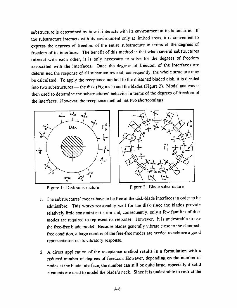
be calculated. To apply the receptance method to the mistuned bladed disk, it is divided

into two substructures -- the disk (Figure 1) and the blades (Figure 2). Modal analysis is

then used to determine the substructures' behavior in terms of the degrees of freedom of

the interfaces. However, the receptance method has two shortcomings:

-q

q-

Figure 1: Disk substructure Figure 2: Blade subswucture

. The substructures' modes have to be free at the disk-blade interfaces in order to be

admissible This works reasonably well for the disk since the blades provide

relatively little constraint at its rim and, consequently, only a few families of disk

modes are required to represent its response. However, it is undesirable to use

the free-free blade model Because blades generally vibrate close to the clamped-

free condition, a large number of the free-free modes are needed to achieve a good

representation of its vibratory response.

. A direct application of the receptance method results in a formulation with a

reduced number of degrees of freedom. However, depending on the number of

nodes at the blade interface, the number can still be quite large, especially if solid

elements are used to model the blade's neck. Since it is undesirable to restrict the

A-3

approachto blademodelswith only a few nodesat the disk-bladeinterface,the

receptance method needs to be modified in order to make it even more efficient.

This is done using the following simplifying assumption.

It is assumed that the disk-blade interfaces undergo rigid body type translations and

rotations. The blade vibration is then determined as a combination of blade base motion

and clamped-free blade modes. As will be shown, this approach results in a formulation

that has a relatively small number of degrees of freedom (six times the number of blades)

and is consequently, computationally efficient. In addition, since the blade's response is

represented in terms of its clamped-free modes its response can be quickly characterized

with only a few modes

MATHEMATICAL FORMULATION

Disk Equation

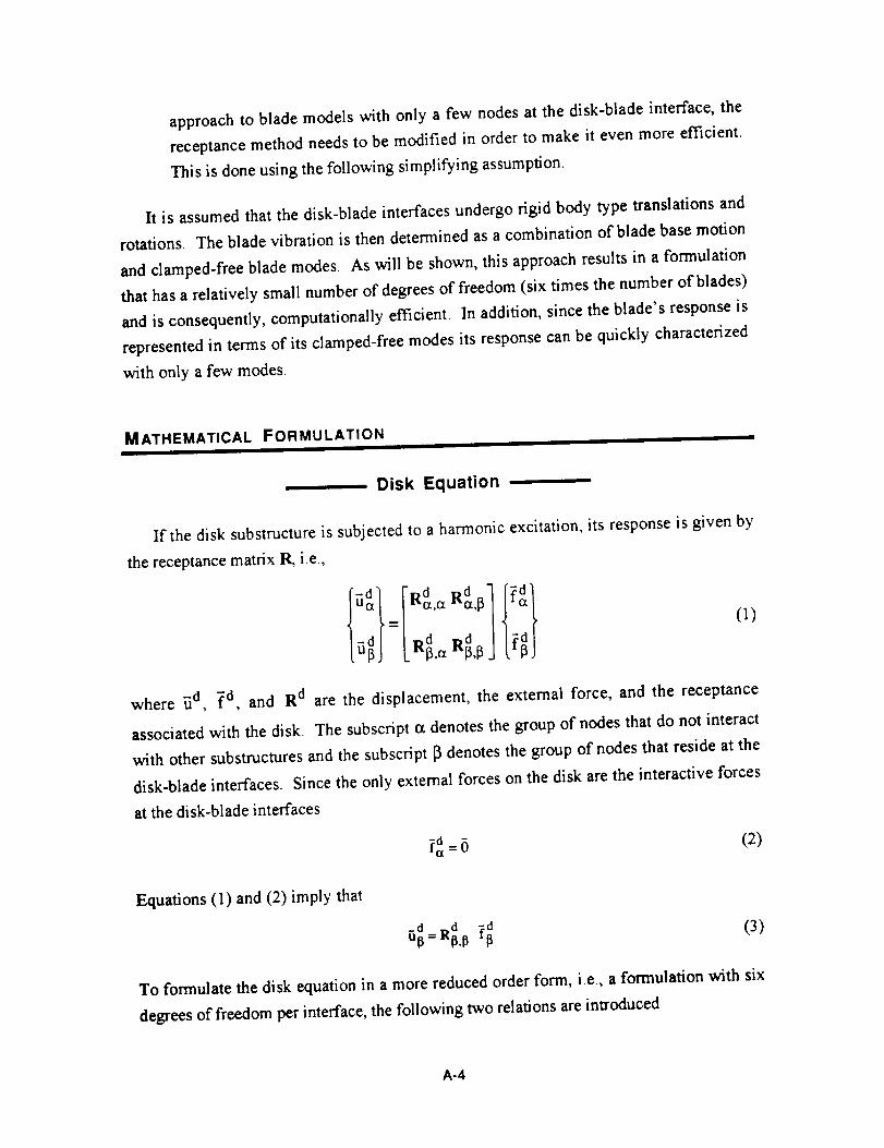
If the disk substructure is subjected to a harmonic excitation, its response is given by

the receptance matrix R, i.e.,

(1)

where _cl, _'d, and R d are the displacement, the external force, and the receptance

associated with the disk. The subscript ot denotes the group of nodes that do not interact

with other substructures and the subscript _ denotes the group of nodes that reside at the

disk-blade interfaces. Since the only external forces on the disk are the interactive forces

at the disk-blade interfaces

-d 6 (2)ftz =

Equations (1) and (2) imply that

To formulate the disk equation in a more reduced order form, i.e., a formulation with six

degrees of freedom per interface, the following two relations are introduced

A-4

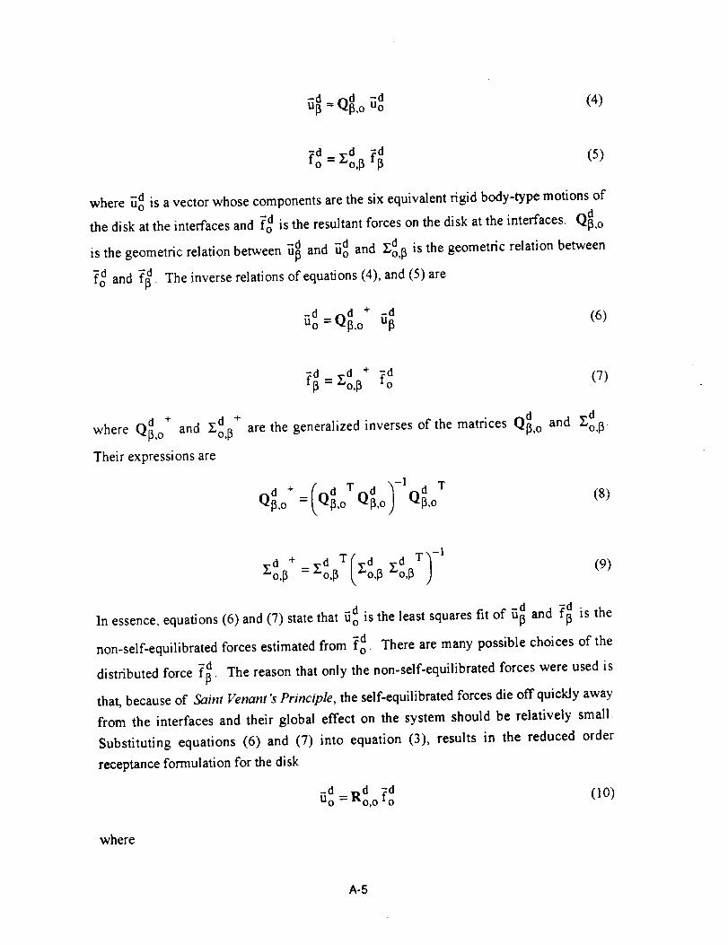
-d d -fo = Zo,13f_ (5)

where rid is a vector whose components are the six equivalent rigid body-type motions of

the disk at the interfaces and _d is the resultant forces on the disk at the interfaces. Q_,o

is the geometric relation between _ and _g and Edo,13is the geometric relation between

?od and f-_. The inverse relations of equations (4), and (5) are

-d d +Uo =QI3,o u (6)

d + d +where Q13,o and Eo,13

Their expressions are

- d + -df_ =Zo,13 fo (7)

d darc the generalizedinversesof the matrices Q13,o and _o,13

d + ( d T d )-IQd TQ13,o = Q13,o 013,o 13,o (8)

d T dd + Y'o,f__(Y'o,f_d T'_-IZo,13 = _o,!3)

(9)

In essence, equations (6) and (7) state that u o is the least squares fit of fi and f is the

-dnon-self-equilibrated forces estimated from fo There are many possible choices of the

distributed force f . The reason that only the non-self-equilibrated forces were used is

that, because of Saint Venant's Principle, the self-equilibrated forces die off quickly away

from the interfaces and their global effect on the system should be relatively small.

Substituting equations (6) and (7) into equation (3), results in the reduced order

receptance formulation for the disk

-d d -dUo =Ro,o fo (10)

where

A-5

d d + od ,-d + (II)Ro,o--Q_.o "13._"o,_

By applying standardmodal analysis,the diskreceptance R_.[3can be writtenas

-d -d T

R_._: Z ¢_j._*_13 (12)

j mj _c0j -.s,! +21flc0j

-d d _ dwhere 0j is thej th disk mode, and m j, _ , and t_j are the modal mass, modal damping

ratio, and natural frequency ofthej th disk mode. Combining equations (11)and (12), the

reduced order disk receptance can be written as

Tj.o , (13)

R°'° = d( d 2 _2 • d

• rnj_.oJj -'_Z +21_j

-d the jth reduced order disk modes, is written aswhere el,o,

_d d + -dj,o =Q_,o Cj._ (14)

Blade Equation

Consider a single blade whose base is constrained to move in a plane undergoing small,

harmonic translations and rotations. Let fib be the six-degree-of-freedom displacement

vector of the blade base and, again, denote the group of nodes that do not interact with the

disk by the subscript o_ and the group of nodes that reside at the interface by [3. The

receptance equation for the blade can be written as

-b_Qb -b b (-b ,2 b Qb -b)ua c_,o Uo = Rot,c_ fct + Ma,cx a,o Uo (15)

-b b -bu_=Q_,o Uo (16)

where _ is the excitation frequency, fib, _b and R b are the displacement, the external

bforce, and the receptance associated with the blade. M_,_ is the blade mass matrix

A-6

associatedwith the group-¢xnodes, b bQet,oand Ql3,oare geometric functions such that

Qb -b b -bct,o uo and QIs.o Uo describe the motion of the entire blade provided that the blade

follows the motion of its base and does not deform. The term 1-22 Mcx,ctbQot,ob uo-bin the

right hand side of equation (15) describes the inertial force introduced by the blade base

motion. Rearranging equation (15), the motion of the group-ct nodes fibct can be expressed-b -b

in terms of the external excitation force fcx and the blade base motion u o, i.e.,

b b -b ( b b ) -bUct Rct,ct fa + _2- = Ra, a Mu,ct + I Qba, o u o

bFrom modal analysis, the receptance Ret,a can be written as

Rct'ct = b( b2 ,-,2 b"7• mj(,toj -_z +2ii)toj

(17)

(18)

-b bwhere Oj is thej th mode for a blade clamped at its base, and m_, _ , and toj are the

modal mass, modal damping ratio, and natural frequency of the jth blade mode.

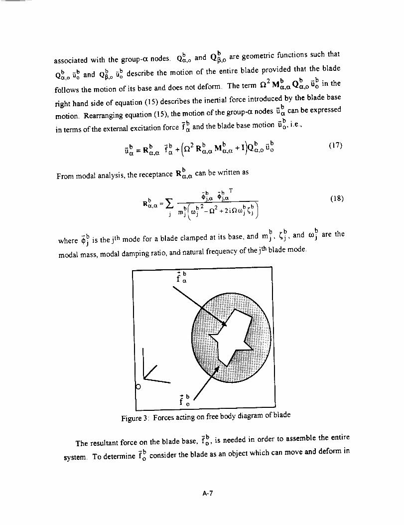
Figure 3: Forces acting on free body diagram of blade

-bThe resultant force on the blade base, fo, is needed in order to assemble the entire

-bsystem. To determine fo consider the blade as an object which can move and deform in

A-7

-bspace(Figure 3). The forces acting on the blade are the excitation force fa and the

-binteractive force at the interface fo. Since linear and angular momentum have to be

conserved, one can deduce that

b(_f_2Mbfib / b_b b-b-bZo _ / = Zo = Zo,c_ fa + fo 09)

bwhere Z o is a geometric function which calculates the resultant force and moment about

-bthe blade base O. Substituting equations (16) and (17) into equation (19), fo can be

h -bexpressed in terms of the blade base motion rio and the external excitation for, i.e.,

-b b -b b -bfo = Zo,o Uo + Ho,ctfa (20)

where

b __2 b b b 4 b b bZo,o _o n Qo-_ zb, ct b= Mct,ct Rct,ctMa,a Qa,o (21)

Hb _2 Zb M b R b Z bo,a=- o,a a,a a,a- o,a (22)

-bEquation (20) describes the relation between the interactive force fo, the blade base

-bmotion Uo, and the external excitation -bfa for a single blade. Clearly, similar equations

apply for all blades. In fact, equations (20), (21) and (22) describe the motions of all of

the blades provided the vectors represent the collections of the corresponding vectors of

individual blades and the matrices become block diagonal matrices with the corresponding

matrices of individual blades at the diagonals.

Assembling the Substructures

Equations (10) and (20) describe the relations between the interactive forces and the

motion of the interfaces for the disk and the blades respectively. Since there are four-d -d -b -b

unknown vectors, Uo, fo, Uo, and fo to be determined, there needs to be two additional

constraints. The first is Newton's law of interactive forces, i.e.,

-d -bfo = -fo (23)

A-8

The second one is Hooke's law which provides a constitutive relation at the interfaces,

i.e.,

-0 (_0_b)fo = Ko,o Uo -Uo (24)

where Ko, o is the stiffness matrix associated with the attachment at the disk-blade

interfaces. I By solving equations (10), (20), (23), and (24) simultaneously, the four-b

unknowns can be expressed in terms of the external excitation force fa, i.e.,

)E -,/1-1b -b-b _( o,o + o,o Zo,o Ho,etUo= R d K -1 l+ b ( o,o+Ko,o fct (25)

-b [ b ( d K-1)1-1 b -bfo = l+Zo, o Ro, o+ o,o Ho,_fa (26)

d I b ( d 1)]-1 b -b-d _Ro, ° +Ko Ho,ct fau o= l+Zo, o Ro, o ,o (27)

-d [ b ( d -1 )1-1 b -b (28)fo = - I + Zo, o Ro, o + Ko, o Ho,a fct

The vibration of the blades can then be easily derived by substituting equation (25) into

equation (I 7).

Remarks on the Mathematical Approach

There are several advantages of using the reduced order formulation (equations (17)

and (25)) to solve the blade mistuning problem:

.

d b bThe coefficient matrices Ro, o, Zo, o, and Ho,a are calculated from the

substructures' modes. Since the frequency range is usually limited to a narrow

range near a particular engine order crossing, only a few dominant modes need to

be included in the calculation and, consequently, the computational cost is low.

1 If the attachment is infinitely stiff, then (24) implies thal the displacements in the blade and disk areequal, and, consequently, (24) becomes a continuity requirement.

A-9

,

.

.

For blade mistuning problems, the disk is treated as a cyclic symmetric structure.

As a result, its modes can be calculated efficiently by applying cyclic symmetric

boundary conditions on a disk segment corresponding to a single blade.

The most computationally intensive pan of this approach lies in computing the

inverse of the matrix l+Zo, o Ro,o+Ko, o in equation (25). This is a square

matrix with dimension six times the number of the blades. In many problems the

rigidity of the disk is such thin only three degrees of freedom are needed to

describe the blade's motion at its base, two rotations and translation normal to the

disk. In either case the number of degrees of freedom are orders of magnitude

smaller than for a finite element model for an entire mistuned bladed disk.

The reduced order method is especially computationally efficient when running

Monte Carlo simulations of blade mistuning since the disk's modes and the

nominal blade's modes need only be calculated once. The coefficient matricesI h b \

f

cantilever blade frequencies in the receptance calculation for each blade. On the

other hand, a direct simulation using finite element models would require

completely new calculations for each mistuned stage.

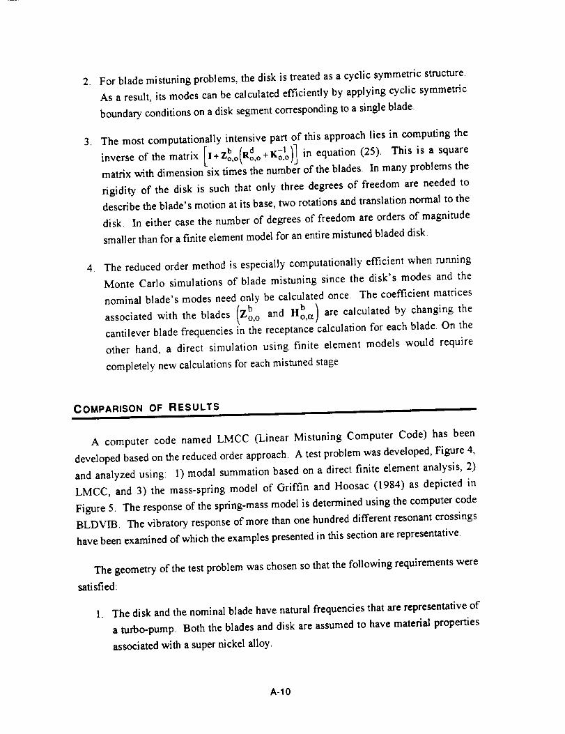
COMPARISON OF RESULTS

A computer code named LMCC (Linear Mistuning Computer Code) has been

developed based on the reduced order approach. A test problem was developed, Figure 4,

and analyzed using: 1) modal summation based on a direct finite element analysis, 2)

LMCC, and 3) the mass-spring model of Griffin and Hoosac (1984) as depicted in

Figure 5. The response of the spring-mass model is determined using the computer code

BLDVIB. The vibratory response of more than one hundred different resonant crossings

have been examined of which the examples presented in this section are representative.

The geometry of the test problem was chosen so that the following requirements were

satisfied:

.. The disk and the nominal blade have natural frequencies that are representative of

a turbo-pump. Both the blades and disk are assumed to have material properties

associated with a super nickel alloy.

A-IO

.

.

The test problem represents a _ m _

realistic three dimensional

structure with low aspect ratio,

plate-like blades. A test problem

consisting of beam-type blades

would not be appropriate since a

goal is to check the validity of the , _

simplifying constraint that the

bases of the blades move as rigid

bodies.

I I

The entire system does not have

too many degrees of freedom, As

a result the entire bladed disk can

be directly analyzed by finite

elements without expending too

much computational time or

having numerical stability

problems.

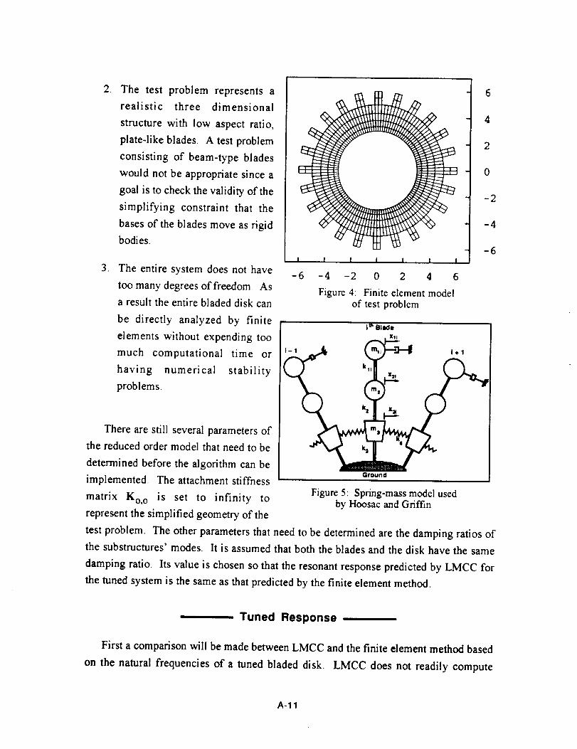
There are still several parameters of

the reduced order model that need to be

determined before the algorithm can be

implemented. The attachment stiffness

matrix Ko, o is set to infinity to

represent the simplified geometry of the

test problem. The other parameters that

the substructures' modes. It is assumed

?

I I

-6 -4 -2 0 2 4 6

Figure 4: Finite element modelof test problem

- 6

- 4

2

0

-2

" --4

-6

ita BlIde

Itll

',,u ,,,

Ground

Figure 5: Spring-mass model usedby Hoosac and Griffin

need to be determined are the damping ratios of

that both the blades and the disk have the same

damping ratio. Its value is chosen so that the resonant response predicted by LMCC for

the tuned system is the same as that predicted by the finite element method.

Tuned Response

First a comparison will be made between LMCC and the finite element method based

on the natural frequencies of a tuned bladed disk. LMCC does not readily compute

A-11

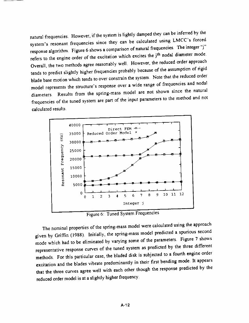
natural frequencies• However, if the system is lightly damped they can be inferred by the

system's resonant frequencies since they can be calculated using LMCC's forced

response algorithm. Figure 6 shows a comparison of natural frequencies. The integer "j"

refers to the engine order of the excitation which excites the jth nodal diameter mode.

Overall, the two methods agree reasonably well. However, the reduced order approach

tends to predict slightly higher frequencies probably because of the assumption of rigid

blade base motion which tends to over constrain the system. Note that the reduced order

model represents the structure's response over a wide range of frequencies and nodal

diameters. Results from the spring-mass model are not shown since the natural

frequencies of the tuned system are part of the input parameters to the method and not

calculated results.

40000

-- 35000N

3O0OO

U

25000

20000

15000

I0000

5000

1 1 J l 1 ! ! i !

Direct FEM -B---

• _ _ _ _ _ _ _ _ _ _

0 1 I I I I f I I I I I

0 1 2 3 4 5 6 7 B 9 I0 Ii 12

Integer j

Figure 6: Tuned System Frequencies

The nominal properties of the spring-mass model were calculated using the approach

given by Griffin (1988). Initially, the spring-mass model predicted a spurious second

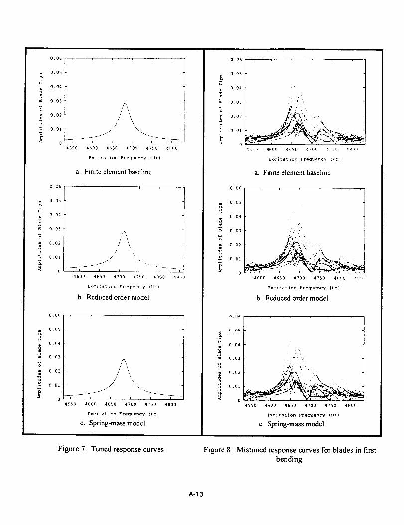
mode which had to be eliminated by varying some of the parameters. Figure 7 shows

representative response curves of the tuned system as predicted by the three different

methods. For this particular case, the bladed disk is subjected to a fourth engine order

excitation and the blades vibrate predominantly in their first bending mode. It appears

that the three curves agree well with each other though the response predicted by the

reduced order model is at a slightly higher frequency.

A-12

13

o

13

.4

Q)13

_D

o

"O

_J

13

X

0.06 ,

0.05 I

0.04

0.03

0.02

0.01

0

4550 4600 4650 4700 4750 4E00

Excitation Frequency (Hz)

a. Finite element baseline

0.06

0.05

0.04

0.03

0.02

0.01

0

l i i l l i

I I I 1 1 I

4600 4650 4700 47%0 4R00 4R_N

E×,"itation Fr_q_onry (Hz)

b. Reduced order model

0.06

0.05 t

0.04

0.03

0.02

0.01

0 I I I I I I I

4550 4600 4650 4700 4750 4R00


c. Spring-mass model

0.06

0 _05

0.04

,--tm 0.03

o

0.02

13

, 0.01

&{-,

13

cD

o

n.

0.06

0.05

0.04

0.03

0.02

0.01

0

0.06

0.05

&

0.04Q13

m 0.03

_40

_, 0.02

13

o.ol

_ o

r v w i 1 I j

• _i,__

. '.% ,; 'i ",

4550 4600 4650 4700 4750 4R00



4600 4650 4700 4750 4£00 4P'_0



4550 4600 4650 4700 4750 4R00



Figure 7: Tuned response curves Figure 8: Mistuned response curves for blades in first

bending

A-13

Mistuned Response

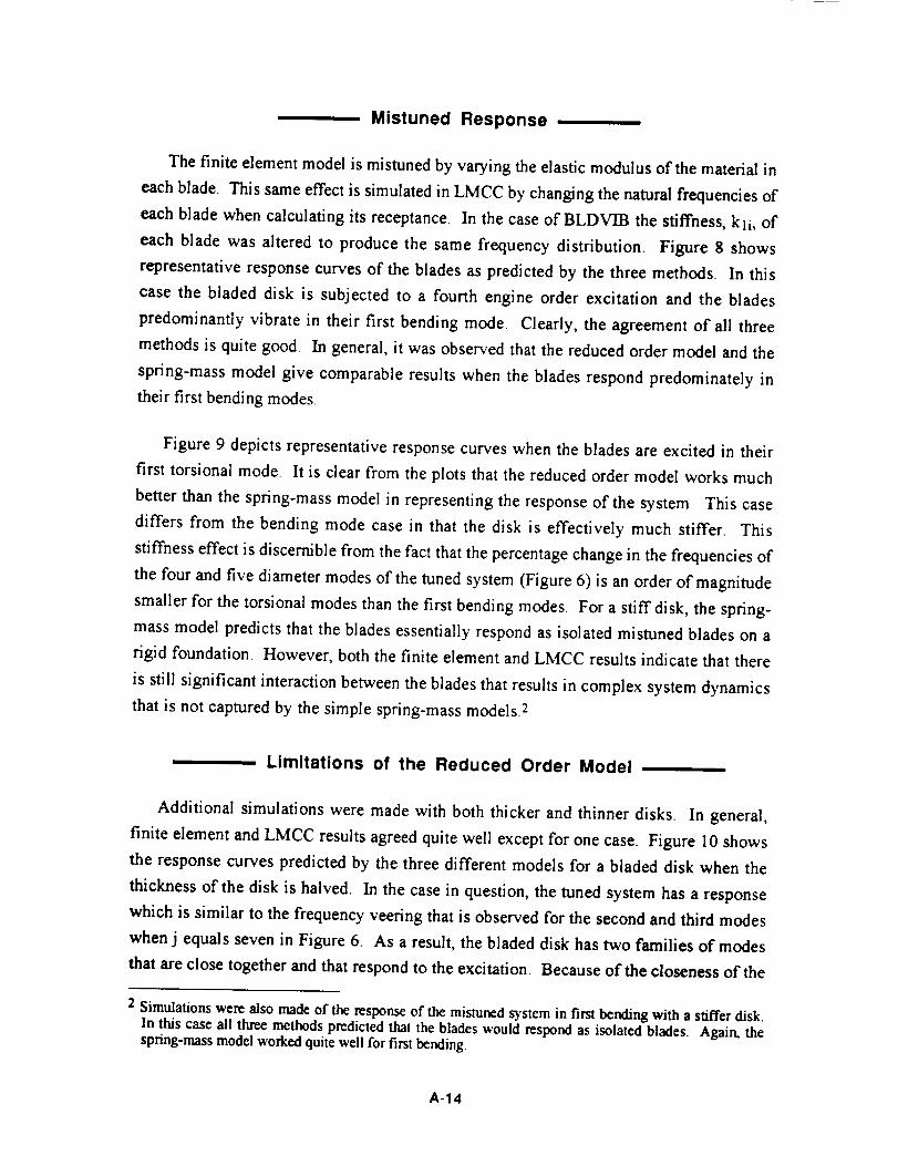
The finite element model is mistuned by varying the elastic modulus of the material in

each blade. This same effect is simulated in LMCC by changing the natural frequencies of

each blade when calculating its receptance. In the case of BLDVIB the stiffness, kli, of

each blade was altered to produce the same frequency distribution. Figure 8 shows

representative response curves of the blades as predicted by the three methods. In this

case the bladed disk is subjected to a fourth engine order excitation and the blades

predominantly vibrate in their first bending mode. Clearly, the agreement of all three

methods is quite good. In general, it was observed that the reduced order model and the

spring-mass model give comparable results when the blades respond predominately in

their first bending modes.

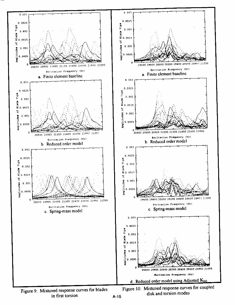
Figure 9 depicts representative response curves when the blades are excited in their

first torsional mode. It is clear from the plots that the reduced order model works much

better than the spring-mass model in representing the response of the system. This case

differs from the bending mode case in that the disk is effectively much stiffer. This

stiffness effect is discernible from the fact that the percentage change in the frequencies of"

the four and five diameter modes of the tuned system (Figure 6) is an order of magnitude

smaller for the torsional modes than the first bending modes. For a stiff disk, the spring-

mass model predicts that the blades essentially respond as isolated mistuned blades on a

rigid foundation. However, both the finite element and LMCC results indicate that there

is still significant interaction between the blades that results in complex system dynamics

that is not captured by the simple spring-mass models2

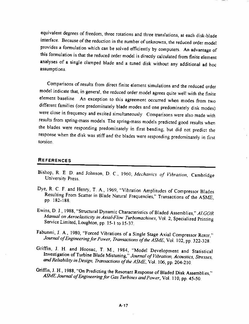
Limitations of the Reduced Order Model

Additional simulations were made with both thicker and thinner disks. In general,

finite element and LMCC results agreed quite well except for one case. Figure l0 shows

the response curves predicted by the three different models for a bladed disk when the

thickness of the disk is halved. In the case in question, the tuned system has a response

which is similar to the frequency veering that is observed for the second and third modes

when j equals seven in Figure 6. As a result, the bladed disk has two families of modes

that are close together and that respond to the excitation. Because of the closeness of the

2 Simulations were also made of the response of the mistuned system in first bending with a stiffer disk.In this case all three methods predicled that the blades would respond as isolated blades. Again, thespring-mass model worked quite well for first bending.

A-14

0.003

0.0025

0.002

0.0015

= o.ooi

0.0005

0

0.003

0.0025

0.002

0,0015

_ 0.001

O,O00S

0

0.003

0,0025

0.002

o.oo15

0.001

o.ooo5

0

J

L :, • ,f .,2 , , ' i .

p

20600 20800 21000 21200 21400 21600 21800 22000

_xc_tation Frequency IHT,)


! v 1 ! i [ i

I20800 21000 21200 21400 21600 21800 22000

Excitation Frequency (Hz_


": 7' '"' '/'' ;q '; _"'. .,%". . . , • • - ,,

20600 20800 21000 21200 21400 21600 21R00 22000


c Spring-mass model

Figure 9: Mistuned response curves for bladesin first torsion

A-15

0.003

ooo2 t0.002

o.oo15

0.001

o.ooos

0

0.003

0.0025

0.002

o.oo1_

o

0.001

3o ooos

0.003

0.0025

P 0.002

0.0015

0.001

0.0005

0

1 i ! i i 1 [ i

19600 19800 20000 20200 20400 20600 20800 21000

Excita£ion Frequency (Hz)


i 1 i i , 1 i I

•L

/ :

t

:• [

ill', ,

_,', L : _// '_,• .'/,:,i.." _ ,.,., , ,,; , •

o20400 20600 20R00 21000 21200 21400 21600 21_00

Excitation Frequency (Hzl


/ }

19600 19800 20000 20200 20400 20600 20800 21000



0.003

0.0025

P 0.002

o.ools

0,001

0.0005

o

...'. :.

:.;"'-:- '_,L ; . ',

; mf . ,"[_m. .. - . "

19600 19800 20000 20200 20400 20600 20800 21000


d Reducedordermodelusin

Figure 10: Mismned response curves for coupleddisk and torsion modes

frequencies, the resulting modes contain significant amounts of both disk and torsional

blade response. It appears that neither the reduced order model nor the spring-mass

model successfully predict the correct results. One problem with the LMCC model is

that it does not predict the separation in the frequencies of the two families of modes

very accurately. This problem was addressed by introducing a finite value of the blade

attachment stiffness matrix, Koo , so that the frequency difference for the tuned system's

response was the same as that of the finite element model. Figure 10(d) shows the

response curves predicted by the reduced order model when the attachment stiffness has

been adjusted. The results from the reduced order model agree somewhat better with the

finite element results, but not as well as in the other cases examined.

Execution Time Comparison

There are two principal advantages of the reduced order model approach which lead to

increased computational efficiency. The first is that the number of degrees of freedom

that must be determined (three or six per blade) in the forced response analysis is

independent of the refinement of the finite element model of the blade and disk models

that are used to calculate its input. Thus, LMCC is especially efficient when compared

to a direct finite element solution of a bladed disk that has a large number of elements.

Secondly, the most computationally expensive part of the calculation with LMCC is in

calculating the modes of the clamped blade and tuned disk using finite elements. Since

this needs to be done only once, LMCC becomes progressively more efficient when more

mistuned bladed disks are simulated in a specific Monte Carlo analysis. An estimate of

the relative run times of LMCC and a finite element analysis using modal superposition

for a representative case indicates that LMCC would be two to three orders of magnitude

faster for a one hundred bladed disk simulation.

CONCLUSIONS

A new reduced order approach has been developed for analyzing the forced response

of mistuned bladed disks. The reduced order model is based on the idea of decomposing

the bladed disk into substructures and representing the response in terms of the degrees of

freedom associated with their interfaces. It further assumes that the blade bases undergo

rigid body-type motions. The blade vibration may then be expressed as a combination of

blade base motion and cantilever blade modes. This approach results in only six

A-16

equivalent degrees of freedom, three rotations and three translations, at each disk-blade

interface. Because of the reduction in the number of unknowns, the reduced order model

provides a formulation which can be solved efficiently by computers. An advantage of

this formulation is that the reduced order model is directly calculated from finite element

analyses of a single clamped blade and a tuned disk without any additional ad hoc

assumptions.

Comparisons of results from direct finite element simulations and the reduced order

model indicate that, in general, the reduced order model agrees quite well with the finite

element baseline. An exception to this agreement occurred when modes from two

different families (one predominately blade modes and one predominately disk modes)

were close in frequency and excited simultaneously. Comparisons were also made with

results from spring-mass models. The spring-mass models predicted good results when

the blades were responding predominately in first bending, but did not predict the

response when the disk was stiff and the blades were responding predominately in first

torsion.

REFERENCES

Bishop, R. E. D. and Johnson, D. C., 1960, Mechanics of Vibration, Cambridge

University Press.

Dye, R. C. F. and Henry, T. A., 1969, "Vibration Amplitudes of Compressor Blades

Resulting From Scatter in Blade Natural Frequencies," Transactions of the ASME,

pp. 182-188.

Ewins, D. J., 1988, "Structural Dynamic Characteristics of Bladed Assemblies," ALGOR

Manual on Aeroelasticity in Axial-Flow Turbomachines, Vol. 2, Specialized Printing

Service Limited, Loughton, pp. 15-1 to 15-37.

Fabunmi, J. A., 1980, "Forced Vibrations of a Single Stage Axial Compressor Rotor,"

Journal of Engineering for Power, Transactions of the ASME, Voi. 102, pp. 322-328.

Griffin, J. H. and Hoosac, T. M., 1984, "Model Development and Statistical

Investigation of Turbine Blade Mistuning," Journal of Vibration, Acoustics, Stresses,

and Reliability in Desig71, Transactions of the ASME, Vol. 106, pp. 204-210.

Griffin, J. H., 1988, "On Predicting the Resonant Response of Bladed Disk Assemblies,"

ASME dournal of Engineering for Gas Turbines and Power, Vol. 110, pp. 45-50.

A-17

Kaza, K. R. V. and Kielb, R. E., 1984, "Flutter of Turbofan Rotors with Mistuned

Blades," A/AA Journal, Vol. 22, No. 11.

Ottarsson, G. and Pierre, C., 1993, "A Transfer Matrix Approach to Vibration

Localization in Mistuned Blade Assemblies," ASME Report No. 93-GT-115,

presented at the International Gas Turbine and Aeroengine Congress and Exposition,

Cincinnati, Ohio, May 24-27.

Rzadkowski, R., 1994, "The General Model of Free Vibrations of Mistuned Bladed

Discs, Part I: Theory," Journal of Sound and Vibration, Vol. 173, No. 3, pp. 377-393.

R.zadkowski, R., 1994, "The General Model of Free Vibrations of Mistuned Bladed

Discs, Part II: Numerical Results," Journal ofSoundand Vibration, Vol. 173, No. 3,

pp. 395-413.

Wagner, L. F., 1993, "Vibration Analysis of Grouped Turbine Blades," Ph.D. Thesis,

Carnegie Mellon University, Pittsburgh, PA.

A-18

APPENDIX B: USER MANUAL FOR LMCC

INTRODUCTION

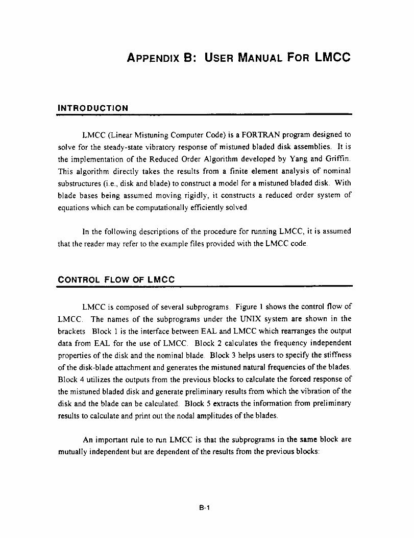
LMCC (Linear Mistuning Computer Code) is a FORTRAN program designed to

solve for the steady-state vibratory response of mistuned bladed disk assemblies. It is

the implementation of the Reduced Order Algorithm developed by Yang and Griffin.

This algorithm directly takes the results from a finite element analysis of nominal

substructures (i.e., disk and blade) to construct a model for a mistuned bladed disk. With

blade bases being assumed moving rigidly, it constructs a reduced order system of

equations which can be computationally efficiently solved.

In the following descriptions of the procedure for running LMCC, it is assumed

that the reader may refer to the example files provided with the LMCC code

CONTROL FLOW OF LMCC

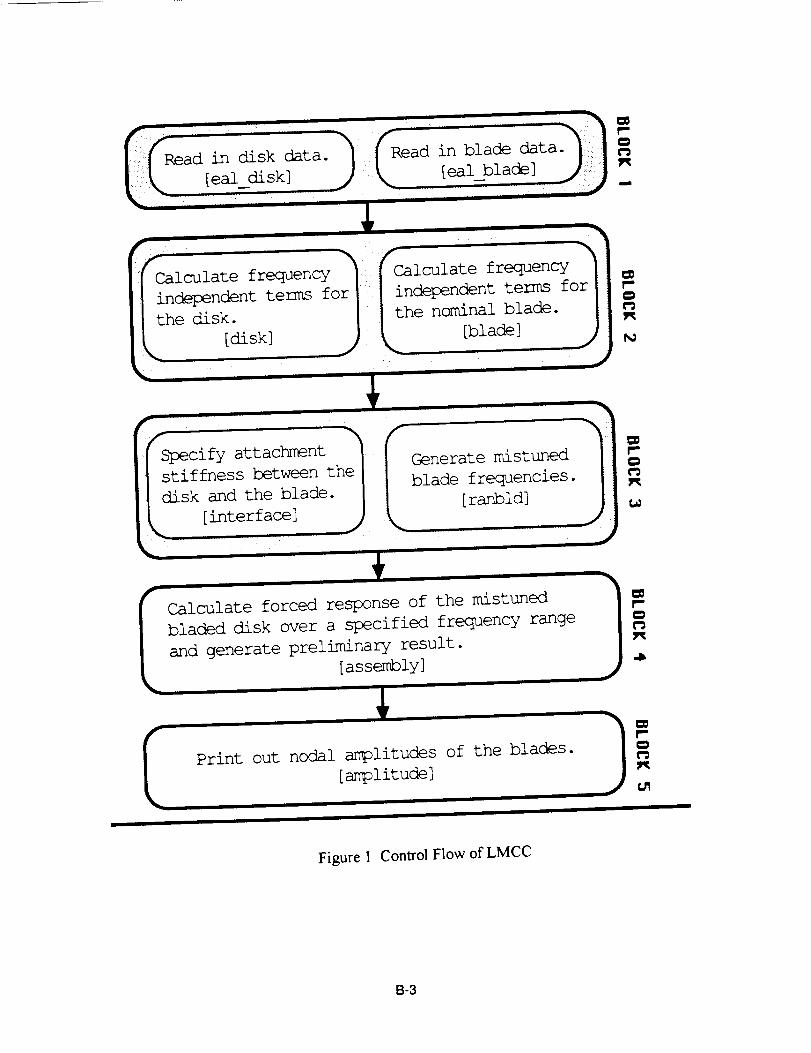
LMCC is composed of several subprograms Figure 1 shows the control flow of

LMCC. The names of the subprograms under the UNIX system are shown in the

brackets. Block 1 is the interface between EAL and LMCC which rearranges the output

data from EAL for the use of LMCC. Block 2 calculates the frequency independent

properties of the disk and the nominal blade. Block 3 helps users to specify the stiffness

of the disk-blade attachment and generates the mistuned natural frequencies of the blades.

Block 4 utilizes the outputs from the previous blocks to calculate the forced response of

the mistuned bladed disk and generate preliminary results from which the vibration of the

disk and the blade can be calculated Block 5 extracts the information from preliminary

results to calculate and print out the nodal amplitudes of the blades.

An important rule to run LMCC is that the subprograms in the same block are

mutually independent but are dependent of the results from the previous blocks:

B-1

Example 1. If a user wants to change the attachment stiffness of the disk-blade

interface but keep analyzing the same set of blades after a certain run, he/she can

just go back to Block 3 to run the subprogram [interface] and run [assembly] in

Block 4 and [amplitude] in Block 5, consequently; he/she does not have to run

[ranbld] in Block 3 or any subprogram in Blocks l and 2.

Example 2. After a certain run, if a user decides that he/she wants to see the

amplitudes of certain blade nodes which were not printed out previously, he/she

only needs to rerun the subprogram [amplitude].

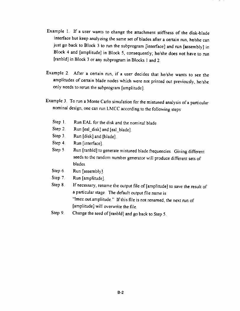
Example 3. To run a Monte Carlo simulation for the mistuned analysis of a particular

nominal design, one can run LMCC according to the following steps:

Step 1.

Step 2.

Step 3.

Step 4.

Step 5.

Step 6.

Step 7.

Step 8.

Step 9.

Run EAL for the disk and the nominal blade.

Run [eal disk] and [eal_blade].

Run [disk] and [blade].

Run [interface].

Run [ranbld] to generate mistuned blade frequencies. Giving different

seeds to the random number generator will produce different sets of

blades.

Run [assembly].

Run [amplitude].

If necessary, rename the output file of [amplitude] to save the result of

a particular stage. The default output file name is

"lmcc.out.amplitude." If this file is not renamed, the next run of

[amplitude] will overwrite the file.

Change the seed of [ranbld] and go back to Step 5

B-2

Calculate frequency Calculate frequency

independent terms for independent terms for

the disk. the nominal blade.

[disk] [blade]

i m ms

Specify attachment h { .

stiffness between thel i Generate mlsttm.eddisk and the blade. J | blade frequencles.

[interface] ] _ [ranbld]

Calculate forced response of the mistuned ]

bladed disk over a specified frequency range I

and generate preliminary result. |

[ass_ly] ,J *

Print out nodal amplitudes of the blades.

[amplitude] ) _I

Figure 1 Con_'ol Flow of LMCC

B-3

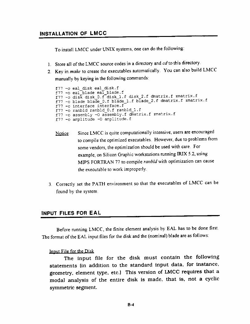
INSTALLATION OF LMCCI

To install LMCC under UNIX systems, one can do the following:

1. Store all of the LMCC source codes in a directory and cdto this directory.

2. Key in make to create the executables automatically. You can also build LMCC

manually by keying in the following commands:

f77 -o eal disk eal disk.f

f77 -o eal blade eal blade.f

f77 -o disk disk O.f disk l.f disk 2.f dmatrix.f zmatrix.f

f77 -o blade blade O.f blade l.f bTade 2.f dmatrix.f zmatrix.f

f77 -o interface interface.f

f77 -o ranbld ranbld O.f ranbld l.f

f77 -o assembly -0 assembly.f dmatrix.f zmatrix.f

f77 -o amplitude -0 amplitude.f

Since LMCC is quite computationally intensive, users are encouraged

to compile the optimized executables. However, due to problems from

some vendors, the optimization should be used with care. For

example, on Silicon Graphic workstations running IRIX 5.2, using

MIPS FORTRAN 77 to compile ra.bld with optimization can cause

the executable to work improperly.

3. Correctly set the PATH environment so that the executables of LMCC can be

found by the system.

INPUT FILES FOR EAL

Before running LMCC, the finite element analysis by EAL has to be done first.

The format of the EAL input files for the disk and the (nominal) blade are as follows:

Innut File for the Disk

The input file for the disk must contain the following

statements {in addition to the standard input data, for instance,

geometry, element type, etc.) This version of LMCC requires that a

modal analysis of the entire disk is made, that is, not a cyclic

symmetric segment.

B-4

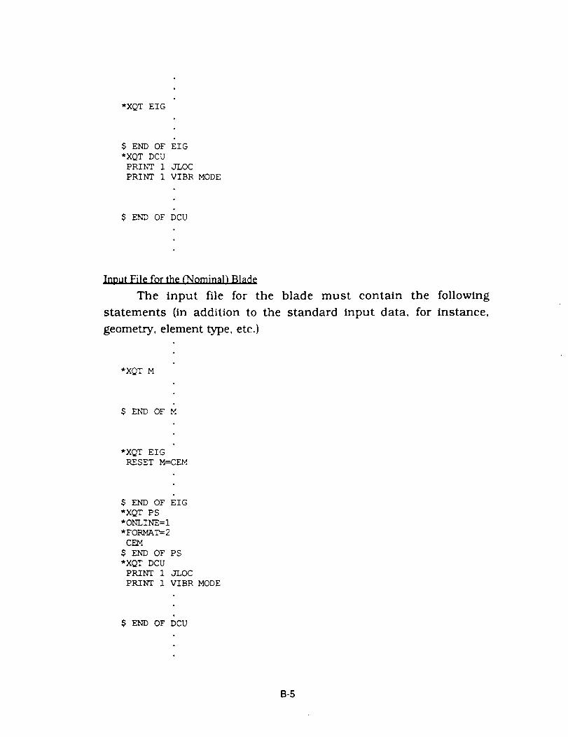
*XQT EIG

$ END OF EIG

*XQT DCU

PRINT 1 JLOC

PRINT 1 VIBR MODE

$ END OF DCU

Input File for the (Nominal) Blade

The input file for the blade must contain the following

statements (in addition to the standard input data, for Instance,

geometry, element type, etc.)

*XQT M

$ END OF M

*XQT EIG

RESET M=CEM

$ END OF EIG

*XQT PS

*ONLINE=I

*FORMAT=2

CEM

$ END OF P S

*XQT DCU

PRINT 1 JLOC

PRINT 1 VIBR MODE

$ END OF DCU

8-5

Notice

1. The execution sequence shown above should be strictly followed. Otherwise,

LMCC will indicate there is an error, The general rule is that the natural

frequencies have to be printed out first (by EIG), then CEM matrix (by PS), then

JLOC (by DCU), and finally VIBR MODE (by DCU).

2. LMCC needs the complete mass matrix of the nominal blade to calculate the

forced response of the system. Since EAL can not print out the moments of

inertia of the nodes while using lumped mass matrix (DEM), LMCC uses the

consistent mass matrix (CEM). Therefore, when running EAL on the blade, one

must use CEM for the analysis.

3. The joint locations (JLOC) and the natural modes (VIBR MODE) have to be put

in Cartesian coordinates. LMCC will not work properly if they are specified in

polar coordinates.

INPUT FILES FOR SUBPROGRAMS OF LMCC

To run the subprograms of LMCC, the associated input files have to be ready

beforehand. There are eight input files corresponding to each of the subprograms

indicated in Figure 1. The input files are named as [subprogram name].m. For example,

the input file name for subprogram ealdisk is ealdisk.m. The input files provide

information which are essential to the forced response analysis and will be read by the

subprograms. The formats of the input files are as follows:

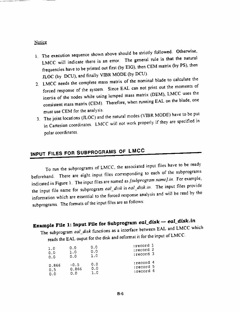
Example File I: Input File for Subprogram eal_.disk- eal_disk.in

The subprogram eal_disk functions as a interface between EAL and LMCC which

reads the EAL ouput for the disk and reformat it for the input of LMCC

1.0 0.0 0.0 :record I

0.0 1.0 0.0 :record 2

0.0 0.0 1.0 :record 3

0.866 -0.5 0.0 :record 4

0.5 0.866 0.0 :record 5

0.0 0.0 1.0 :record 6

B-6

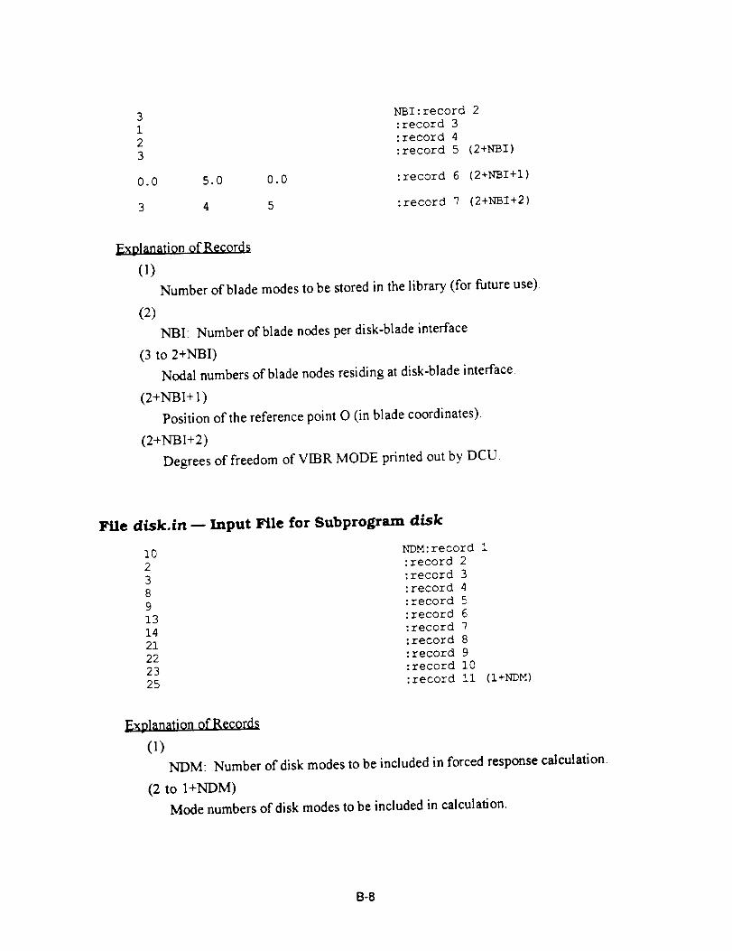
3 NDI :record 7

481 :record 8

482 :record 9

483 :record i0 (7+NDI)

0.0 5.0 0.0 :record ii (7+NDI+I)

I0 :record 12 (7+NDI+2)

45 :record 13 (7+NDI+3)

12 :record 14 (7+NDI+4)

3 4 5 :record 15 (7+NDI+5)

Extflanation of RecQrds

(] to 3)Matrix of direction cosines which transfers the disk coordinates to the first

blade coordi nares

(4 to 6)

Matrix of direction cosines which transfers the ith blade coordinates to the

(i+l)th blade coordinates.

(7)

NDI: Number of disk nodes per disk-blade interface.

(8 to 7+NDI)

Nodal numbers of disk nodes residing at the first disk-blade interface.

(7+NDI+ 1)

Position &the reference point O (in disk coordinates) associated with the first

blade.

(7+NDI+2)

Nodal number difference between corresponding disk nodes residing at

neighboring interfaces.

(7+NDI+3)

Number of disk modes to be stored in the library (for future use).

(7+ND+4)

Number of blades.

(7+ND+5)

Degrees of freedom of VIBR MODE printed out by DCU.

File eal_blade.in- Input File for Subprogram ea!blade

i0 :record 1

8-7

3 NBI:record 2

1 :record 3

2 :record 4

3 :record 5 (2+NBI)

0.0 5.0 0.0 :record 6 (2+NBI+I)

3 4 5 :record 7 (2+NBI+2)

Explanation of Records

(1)

(2)

Number of blade modes to be stored in the library (for future use).

NBI: Number of blade nodes per disk-blade interface.

(3 to 2+NBI)

Nodal numbers of blade nodes residing at disk-blade interface,

(2+NBI+ 1 )

Position of the reference point 0 (in blade coordinates).

(2+NBI+2)

Degrees of freedom of VIBR MODE printed out by DCU.

File disk.in _ Input File for Subprogram disk

I0 NDM:record 1

2 :record 2

3 :record 3

8 :record 4

9 :record 5

13 :record 6

14 :record 7

21 :record 8

22 :record 9

23 :record i0

25 :record Ii (I+NDM)


(1)

NDM: Number of disk modes to be included in forced response calculation.

(2 to I+NDM)

Mode numbers of disk modes to be included in calculation.

8-8

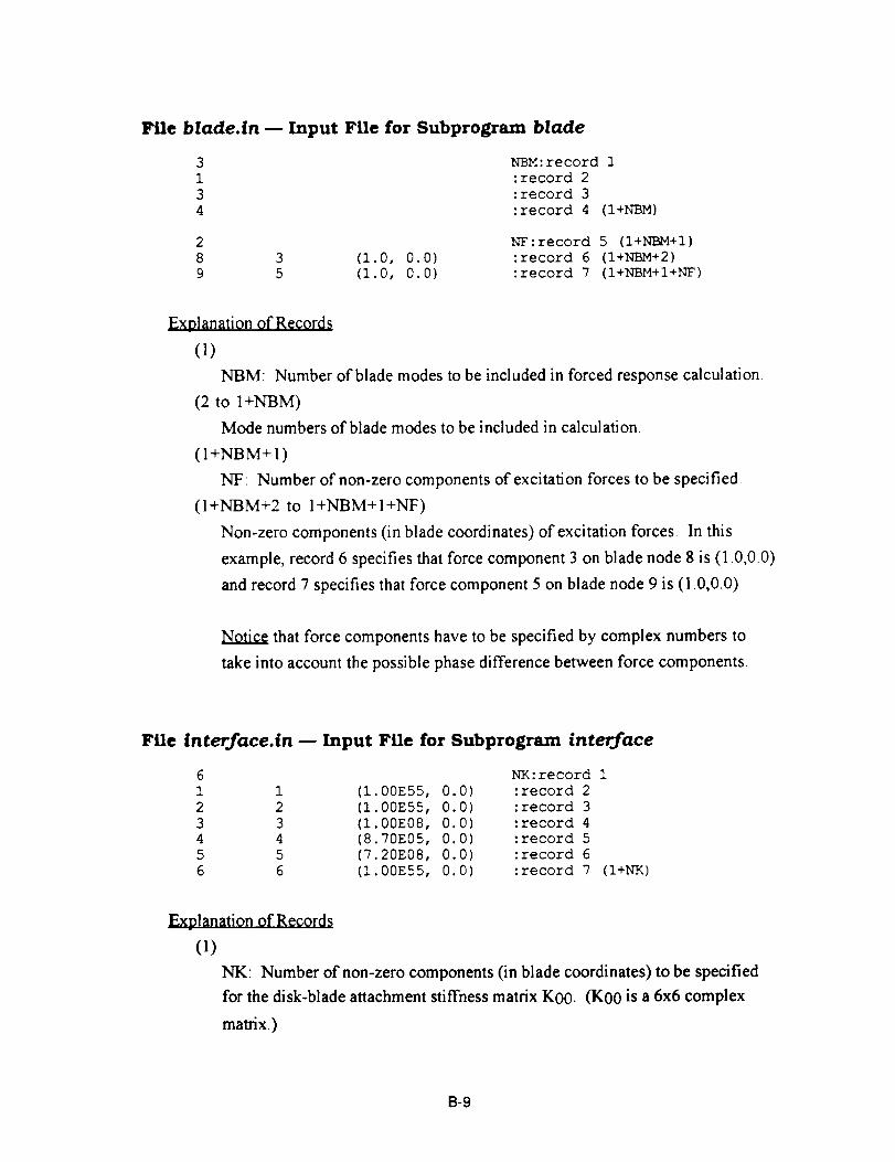
File blade.in m Input File for Subprogram blade

3 NBM:record 1

1 :record 2

3 :record 3

4 :record 4 (I+NBM)

2 NF: record 5 (I+NI_4+I)

8 3 (I.0, 0.0) :record 6 (I+NBM+2)

9 5 (I.0, 0.0) :record 7 (I+NBM+I+NF)


(1)

NBM: Number of blade modes to be included in forced response calculation.

(2 to I+NBM)

Mode numbers of blade modes to be included in calculation.

(I+NBM+I)

NF: Number of non-zero components of excitation forces to be specified.

(I+NBM+2 to I+NBM+I+NF)

Non-zero components (in blade coordinates) of excitation forces. In this

example, record 6 specifies that force component 3 on blade node 8 is (1.0,0.0)

and record 7 specifies that force component 5 on blade node 9 is (I .0,0.0).

Notice that force components have to be specified by complex numbers to

take into account the possible phase difference between force components.

File interface.in- Input File for Subprogram interface

6

1 1 (i

2 2 (i

3 3 (i

4 4 (8

5 5 (76 6 (i

NK:record 1

00E55, 0.0) :record 2

00E55, 0.0) :record 3

00E08, 0.0) :record 4

70E05, 0.0) :record 5

20E08, 0.0) :record 6

00E55, 0.0) :record 7 (I+NK)


(1)

NK: Number of non-zero components (in blade coordinates) to be specified

for the disk-blade attachment stiffness matrix K00. (K00 is a 6x6 complex

matrix.)

B-9

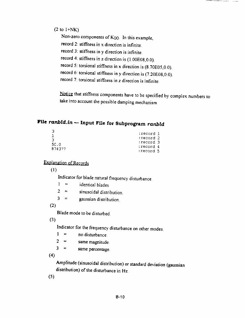
(2 to I+NK)

Non-zero components ofK00. In thisexample,

record2:stiffnessinx directionisinfinite.

record3:stiffnessiny directionisinfinite.

record4: stiffnessin z directionis(1.00E08,0.0).

record5:torsionalstiffnessinx directionis(8.70E05,0.0).

record6:torsionalstiffnessiny directionis(7.20E08,0.0).

record 7:torsionalstiffnessinz directionisinfinite.

Notice that stiffness components have to be specified by complex numbers to

take into account the possible damping mechanism.

File ranbld.in _ Input File for Subprogram ranbld

3 :record 1

1 :record 2

3 :record 3

50.0 :record 4

874377 :record 5

Explanation of Recor4_

(i)

(2)

(3)

(4)

(5)

Indicator for blade natural frequency disturbance,

1 = identical blades.

2 = sinusoidal distribution.

3 = gaussian distribution.

Blade mode to be disturbed.

Indicator for the frequency disturbance on other modes.

1 = no disturbance.

2 = same magnitude,

3 = same percentage.

Amplitude (sinusoidal distribution) or standard deviation (gaussian

distribution) of the disturbance in Hz.

B-lO

Number of nodal diameters ofsinusoidal distribution or seed for the gaussian

random number generator.

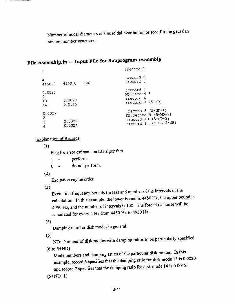
File assembly.in _ Input File for Subprogram assembly

1 :record 1

4 :record 2

4450.0 4950.0 I00 :record 3

0.0025 :record 4

2 ND:record 5

13 0.0020 :record 6

14 0.0015 :record 7 (5+ND)

0.0027 :record 8 (5_ND+I)

2 NB:record 9 (5+ND+2)

3 0.0022 :record I0 (5+ND+3)

4 0.0024 :record ii (5+ND+2+NB)

ExDlanation of Records

(1)

Flag for error estimate on LU algorithm.

1 = perform.

0 = do not perform.

(2)

(3)

(4)

(5)

Excitation engine order.

Excitation frequency bounds (in Hz) and number of the intervals of the

calculation. In this example, the lower bound is 4450 Hz, the upper bound is

4950 Hz, and the number of intervals is 100. The forced response will be

calculated for every 4 Hz from 4450 Hz to 4950 Hz.

Damping ratio for disk modes in general.

ND: Number of disk modes with damping ratios to be particularly specified.

(6 to 5+ND)

Mode numbers and damping ratiosofthe particulardiskmodes. In this

example, record 6 specifies that the damping ratio for disk mode 1:3 is 0.0020

and record 7 specifies that the damping ratio for disk mode 14 is 0.0015.

(5+ND+I)

B-11

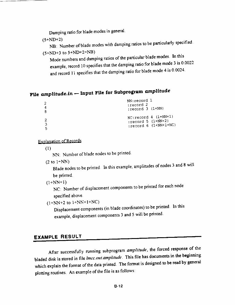
Damping ratio for blade modes in general.

(5+ND+2)

NB: Number of blade modes with damping ratios to be particularly specified.

(5+ND+3 to 5+ND+2+NB)

Mode numbers and damping ratios of the particular blade modes. In this

example, record 10 specifies that the damping ratio for blade mode 3 is 00022

and record 11 specifies that the damping ratio for blade mode 4 is 0.0024.

File amplitude.in m Input File for Subprogram amplitude

2 NN:record 1

4 :record 2

8 :record 3 (I+NN)

2 NC:record 4 (I+NN+!)

3 :record 5 (I+NN÷2)

5 :record 6 (I+NN+I+NC)

Ext31anation of Records

(I)

NN: Number of blade nodes to be printed.

(2 to I+NN)

Blade nodes to be printed. In this example, amplitudes of nodes 3 and 8 will

be printed.

(I+NN+I)

NC: Number of displacement components to be printed for each node

specified above.

(I+NN+2 to I+NN+I+NC)

Displacement components (in blade coordinates) to be printed. In this

example, displacement components 3 and 5 will be printed.

EXAMPLE RESULTI I I

After successfully running subprogram amplitude, the forced response of the

bladed disk is stored in file lmcc.out.amplitude. This file has documents in the beginning

which explain the format of the data printed. The format is designed to be read by general

plotting routines. An example of the file is as follows:

B-12

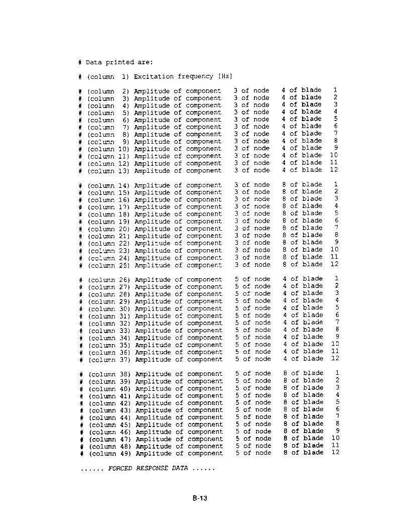
# Data printed are:

# (column i) Excitation frequency [Hz]

# (column

# (column

# (column

# (column 5

# (column 6

# (column 7

# (column 8

# (column 9

# (column I0

# (column II

# (column 12

# (column 13

2) Amplitude of component

3) Amplitude of component

4 Amplitude of component

Amplitude of component









# (column 14) Amplitude of component


# (column 167 Amplitude of component










# (column 26

# (column 27

# (column 28

# (column 29

# (column 30

# (column 31

# (column 32

# (column 33

# (column 34

# (column 35

# (column 36

# (column 37

























...... FORCED RESPONSE DATA ......

3 of node

3 of node

3 of node

3 of node

3 of node

3 of node

3 of node

3 of node

3 of node

3 of node

3 of node

3 of node

3 of node

3 of node

3 of node

3 of node

3 of node

3 of node

3 of node

3 of node

3 of node

3 of node

3 of node

3 of node

5 of node

5 of node

5 of node

5 of node

5 of node

5 of node

5 of node

5 of node

5 of node

5 of node

5 of node

5 of node

5 of node

5 of node

5 of node

5 of node

5 of node

5 of node

5 of node

5 of node

5 of node

5 of node

5 of node

5 of node

4 of blade 1

4 of blade 2

4 of blade 3

4 of blade 4

4 of blade 5

4 of blade 6

4 of blade 7

4 of blade 8

4 of blade 9

4 of blade I0

4 of blade Ii

4 of blade 12

8 of blade 1

8 of blade 2

8 of blade 3

8 of blade 4

8 of blade 5

8 of blade 6

8 of blade 7

8 of blade 8

8 of blade 9

8 of blade i0

8 of blade ii

8 of blade 12

4 of blade 1

4 of blade 2

4 of blade 3

4 of blade 4

4 of blade 5

4 of blade 6

4 of blade 7

4 of blade 8

4 of blade 9

4 of blade I0

4 of blade II

4 of blade 12

8 of blade 1

8 of blade 2

8 of blade 3

8 of blade 4

8 of blade 5

8 of blade 6

8 of blade 7

8 of blade 8

8 of blade 9

8 of blade i0

8 of blade ii

8 of blade 12

B-13

°owo°°°o°°,°°m°o°°o°°°°°,o°.°°o°o°

°o,°o°°o°°,°op°o°°oo°oo°oo°°°°°°o°

ADDITIONAL CONSIDERATION AND POTENTIAL PROBLEMSI

While using EAL as the preprocessor of LMCC, we found that EAL occasionally

generates disk modes which are not mutually orthogonal. The problem was that modes of

the same number of nodal circles and same number of nodal lines should have the same

mode shape except that they are out of phase. EAL sometimes generates this kind of

modes with correct mode shapes which are not completely out of phase. This kind of

error causes the forced response calculation so that LMCC will give meaningless results.

Typically when this error occurs, it is indicated by the fact that LMCC predicts

unusually high forced response over part of the frequency range

B-14

Appendix C: Theoretical Manual for LMCC

ABSTRACT1

This appendix contains the theory of the reduced order algorithm upon which the Linear

Mistuning Computer Code (LMCC) is based. Chapter 1 is the introduction and motivation of

this research project. Chapter 2 and Chapter 3 state the theory of the reduced order

algorithm. Chapter 4 gives some benchmark test cases and the comparison between the

reduced order model and the traditional spring-mass model.

Chapter 1: INTRODUCTION AND MOTIVATIONI

In the use ofturbomachinery in modem aircraft, blades have failed from high cycle fatigue

because of excessive vibration. Based on experiments and earlier analytical investigations

[1-5], it is realized that, because of the rotational periodicity of its geometry, a bladed disk

usually has natural frequencies that are clustered in narrow ranges. When the natural

frequencies of a system are close together, slight variations in the system's structural

properties can cause large changes in its modes, and, consequently, its dynamic response. The

sensitivity of a bladed disk's dynamic response to small variations in the frequencies of the

blades is referred to in the literature as the "blade mistuning problem" and has been studied

extensively. It is important to understand mistuning since it can result in large blade to blade

variations and the high response blades can fail from high cycle fatigue. For modem aircraft,

such as a space shuttle, the high vibratory response of bladed disks is of special concern

because of the severe operating conditions to which they are subjected.

Every year, a great number of experiments are conducted by industry to ensure that the

blades are safely designed. These experiments are generally expensive and time-consuming In

order to reduce the time and cost associated with these experiments, turbine manufacturers

replace part of the experiments by numerical simulations. From a modeling point of view,

traditional simulations can be classified into several categories. One of them is to directly use

finite element methods. The direct finite element approach is straight forward and can

C-1

accurately model the characteristics of a structure provided that the structure is represented

with enough elements, However, since a structurally accurate finite element model for a

typical bladed disk can have more than 1,000,000 degrees of freedom, the associated

computational time for deriving the eigenvalues and eigenvectors of a single stage can be as

high as 1,000 CPU minutes on a CRAY. Ifa thorough mistuning analysis using Monte Carlo

Simulation is desired, the total CPU time it consumes will be prohibitively high. (For

example, 100,000 CPU minutes for a 100 stage simulation,) In addition, the extremely large

memory requirements for data storage and the numerical errors associated with numerical

instabilities make the direct finite element approach unfeasible.

There have been attempts to develop structurally accurate models for bladed disks.

Reference may be made to a feature article by Leissa [10], in which, the progress in modeling

blades for vibration analyses is discussed. Many of the attempts to develop structurally

accurate models for bladed disks use plate elements to represent the disk and beam elements

to represent the blades [3,11-13,21]. While there can be blade configurations for which the

beam representation may be adequate, plate, thick shell, and even solid elements are often

needed to represent modem, low aspect ratio blades. With recent improvements in finite

element methods and computer speed, a whole bladed disk could be modeled accurately but,

as previously mentioned, it is recognized that the cost of running these programs would be

prohibitively high for use during the design process. This leads to the attempts by researchers

to use substructuring techniques in which results from finite element analyses of individual

substructures are used to obtain the dynamic behavior of the whole bladed disk [14,15].

There have also been attempts to introduce the cyclic symmetric boundary conditions into

finite element codes to model bladed disks so that the system modes can be efficiently solved

for and, because of the clustered natural frequencies being separated, the numerical stability is

improved [7,16,17].

While finite element models with cyclic symmetric boundary conditions can be easily

solved for tuned bladed disks, much of the work that has been done in mistuning utilizes

spring-mass models to represent the bladed disk [ 1,2,4,8,18-21] in order to reduce the number

of degrees of freedom and to make the problem computationally more tractable. While they

may often provide reasonably accurate predictions of the system's response, the model's

parameters, such as the mass and the spring constants, are usually chosen in an ad hoc manner

and one must question the ability of such simple models to accurately represent such complex

systems. Little work has been published which verifies their accuracy.

C-2

The goal of this researchis to developa methodologythat will directly take the results

from a finite elementanalysisof a tuned systemand constructa computationallyefficientmistunedmodelwith a reducednumberof degreesof freedom.Theintentis thattheapproach

will display thestructuralaccuracyof thefinite elementmodeland computationalefficiency

comparableto a spring-massmodel.

Chapter 2: RECEPTANCE METHOD AND REDUCED ORDER

MODELING

2.1 Receptance Method

In structural dynamics, one widely used analytical method is to subdivide a complex

structure into several substructures, analyze the behavior of the individual substructures, and

then use the receptance method [6] to reassemble the structure. Receptance method is based

on the observation that, for every substructure, the dynamic response is determined by how

the substructure interacts with its environment. If the substructure interacts with its

environment only at a limited number of interfaces, it is possible to express the degrees of

freedom of the entire substructure in terms of the degrees of freedom of these interfaces. The

benefit of this method is that when several substructures interact with each other, we only

need to solve for the degrees of freedom of the interfaces. Once the degrees of freedom of

these interfaces are determined the response of all substructures and, therefore, the whole

structure is known.

To apply the receptance method to a bladed disk, let us consider the disk and all of the

blades as two separate substructures. We can then write the receptance equations for the disk

and the blades

--du =R d(2.1)

;b=Rbfb(2.2)

--d --dwhere u , f ,andR d are the displacement, the external force, the receptance associated with

the disk, and u°-°, f , and R b are the displacement, the external force, and the receptance

C-3

associated with the blades, By denoting the group of nodes which do not interact with the

other substructure by _t, and the group of nodes which are residing at the interfaces by 13, we

can write equations (2.1) and (2.2) in components,

"'dHa

u_

Rd Rd 1

R dl_,a Rdl_&J

(2.3)

-"bHaRb Rb 1.-- _,ff. a,13

R e13,_R_,13I

(2.4)

Since, in general, the only external forces on the disk are the interactive forces at the disk-blade

interfaces, we assume that

(2.5)

Furthermore, if we assume the excitation forces on the blades are prescribed, then, by

requiting the displacements to be continuous and the interactive forces to follow Newton's

Interactive Force Law,

(2.6)

(2.7)

we can solve for the forces at the interfaces using equations (2.3) and (2.4)

13= - R ,1_+ R ,13 13,ctfcx (2.8)

and

13= R ,13+ R ,13 I_,ctf a (2.9)

-'b -*d

Since the only unknowns on the tight hand sides of equations (2.3) and (2.4) are f 13and f 13,

the response of the entire bladed disk is known.

C-4

The benefit of using equations (2.8) and (2.9) is that we only need to solve the problem in

the subspace-13 without the necessity of either calculating the inverse of the dynamic

impedance of the whole bladed disk or finding the modes for the entire system. However,

finding the receptances for the disk and the blades beforehand still can be computationally

intensive. A mathematical expression for the receptances of the disk and the blades are

R o ={K d __2 M o + i_ C'd) -1

R b ={K b -f2 2 M b + if2 Cb) -I

(2.10)

(2.11)

where K d, M d, and C d are the stiffness, mass, and damping matrices of the disk, and K b,

M b, and Cb are the stiffness, mass, and damping matrices of the blades, i'2 is the excitation

frequency. R b is a block-diagonal matrix if there is no structural links between the blades.

An alternative way of calculating these receptances is to use the substructures' modes.

That is, by applying standard modal analysis, the receptances can be written in the following

form

Rd =E

.-. b .-. b T

Rb =E 0j t_j

J m_ mb2 ;-n +2in_

-d d d d

where _bj, m j, _ j, and co j are the mode shape, modal mass, modal damping ratio, and naturalb b b b

frequency of the j-th disk mode, and ¢?j, m j, r_-j, and o)j are the mode shape, modal mass,

modal damping ratio, and natural frequency of the j-th blade mode, respectively. This method

is in general better that equations (2.10) and (2.11) since, with the substructures' modes

derived in advance, using equations (2.12) and (2.13) to calculate the receptances needs merely

algebraic multiplications and additions, whereas equations (2.10) and (2.1 l) involve the

calculation of matrix inverses for every excitation frequency. The other benefit of equations

(2.12) and (2.13) is that not all of the substructures' modes are needed in the calculation.

Since the modes with natural frequencies close to the excitation frequency will dominate the

(3-5

response,the othermodescanbeeliminatedfrom thecalculationwithout a significantlossof

accuracy

However, there are still several shortcomings which prevent us from using the receptance

formulation (the combination of equations (2.8), (2.9), (2.12), and (2.13)) to solve our

problem:

1. The substructures' modes used in equations (2.12) and (2.13) have to be free at the

disk-blade interfaces, or, in other words, they have to be admissible. To satisfy this

requirement, it is fine for us to use the disk modes which are clamped at the inner edge

and free at the outer edge, but it is undesirable to use the free-free blade modes.

Because the blades generally vibrate close to the clamped-free condition, we need a

large number of the free-free modes to achieve a good representafi on of blade vibration.

Another more realistic reason for not using free-free blade modes is that most of the

analyses done on the blades in the industry, either numerically or experimentally, use

cantilever blades. There is much more information available on the clamped-free blades

than the free-free blades.

2. In equations (2.8) and (2.9), we need to find the inverse of the matrix R ,8 + R 1_,13•

This matrix has a dimension of the group-_3 nodes which is much smaller than the

dimension of the whole bladed disk, but, still, there can be too many degrees of

freedom to be solved for. Since we do not want to restrict our analysis to use a

particular type of blade models, for example, beam-type blade model with single-node

contact at the disk-blade interface, we need to modify the receptance method to have

the capability to handle multiple-point disk-blade attachments.

2.2 Reduced Order Modeling Based On Rigid Blade Base

Assumption

One of the reasons that the direct receptance method is not particularly attractive is that

there are still too many degrees of freedom. In this section, we would like to propose a

reduced order method which is capable of handling multiple-point disk-blade attachments and,

yet, results in a formulation having fewer degrees of freedom.

C-6

For a system of substructures having multiple point contact with each other, it is in

general not possible to reduce the number of degrees of freedom of its receptance formulation.

However, for a bladed disk, the deformation of the disk-blade interfaces is in general not

significant in Comparison with the deformation of the blades. Therefore, except for the case

when the high nodal diameter disk modes strongly participate, each of the blade bases can be

reasonably approximated by six degrees of freedom, namely, three translations and three

rotations. With this assumption, the number of degrees of freedom of the reduced order

formulation will be six times of the number of blades which is much smaller than that of the

direct receptance formulation.

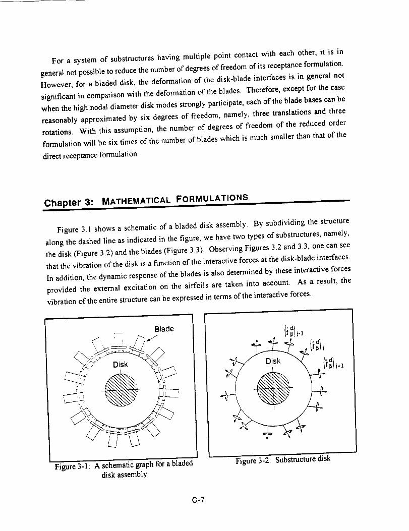
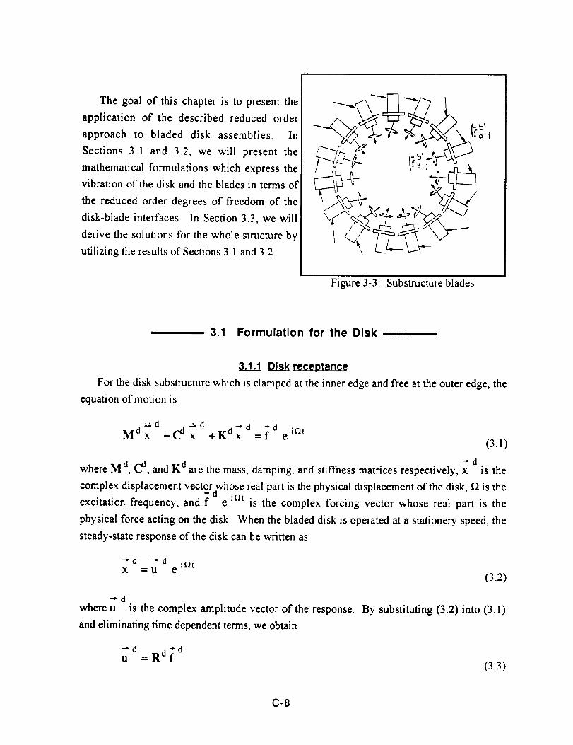
Chapter 3: MATHEMATICAL FORMULATIONSi i

Figure 3.1 shows a schematic of a bladed disk assembly. By subdividing the structure

along the dashed line as indicated in the figure, we have two types of substructures, namely,

the disk (Figure 3.2) and the blades (Figure 3.3). Observing Figures 3.2 and 3.3, one can see

that the vibration of the disk is a function of the interactive forces at the disk-blade interfaces.

In addition, the dynamic response of the blades is also determined by these interactive forces

provided the external excitation on the airfoils are taken into account. As a result, the

vibration of the entire structure can be expressed in terms of the interactive forces.

Blade

_ , ! J

Figure 3-1: A schematic graph for a bladed

disk assembly

Figure 3-2: Substructure disk

C-7

The goal of this chapter is to present the

application of the described reduced order

approach to bladed disk assemblies. In

Sections 3.1 and 3.2, we will present th_

mathematical formulations which express th_

vibration of the disk and the blades in terms of

the reduced order degrees of freedom of the

disk-blade interfaces. In Section 3.3, we will

derive the solutions for the whole structure by

utilizing the results of Sections 3. l and 3.2.

Figure 3-3 Substructure blades

3.1 Formulation for the Disk

3.1.1 Disk rct,.e. a

For the disk substructure which is clamped at the inner edge and free at the outer edge, the

equation of motion is

._d -_d -'d -'d iflt

Mdx +C 'd x +Kdx =f e (3.1)

"-'dwhere M d, C-d, and K d are the mass, damping, and stiffness matrices respectively, x is the

complex displacement vector whose real part is the physical displacement of the disk, fl is the"" d iflt

excitation frequency, and f e is the complex forcing vector whose real part is the

physical force acting on the disk. When the bladed disk is operated at a stationery speed, the

steady-state response of the disk can be written as

"" d -" d i_tX =U e

(3.2)

"d

where u is the complex amplitude vector of the response.

and eliminating time dependent terms, we obtain

By substituting (3.2) into (3.1)

d=Rdfd(3.3)

C-8

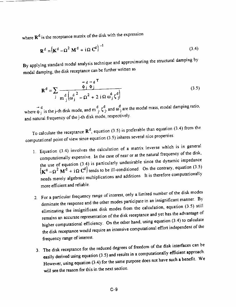
where R d is the receptance matrix of the disk with the expression

(3.4)

By applying standard modal analysis technique and approximating the structural damping by

modal damping, the disk receptance can be further written as

.-. d .-. d T

(3.5)

where g_j is the j-th disk mode, and m , _ , and co j are the modal mass, modal damping ratio,

and natural frequency of the j-th disk mode, respectively.

To calculate the receptance R d, equation (3.5) is preferable than equation (3.4) from the

computational point of view since equation (3.5) inheres several nice properties:

. Equation (3.4) involves the calculation of a matrix inverse which is in general

computationally expensive. In the case of near or at the natural frequency of the disk,

the use of equation (3.4) is particu/arly undesirable since the dynamic impedance

(KCl _f12 M _ + if_ C-d} tends to be ill-conditioned. On the contrary, equation (3.5)

needs merely algebraic multiplications and additions. It is therefore computationally

more efficient and reliable.

. For a particular frequency range of interest, only a limited number of the disk modes

dominate the response and the other modes participate in an insignificant manner. By

eliminating the insignificant disk modes from the calculation, equation (3.5) still

remains an accurate representation of the disk receptance and yet has the advantage of

higher computational efficiency. On the other hand, using equation (3.4) to calculate

the disk receptance would require an intensive computational effort independent of the

frequency range of interest.

. The disk receptance for the reduced degrees of freedom of the disk interfaces can be

easily derived using equation (3.5) and results in a computationally efficient approach.

However, using equation (3.4) for the same purpose does not have such a benefit. We

will see the reason for this in the next section.

C-9

Disk _ at the disk-blade Interlaces

As was mentioned in Chapter 2, the response of the disk is a function of the interactive

forces that act between the disk and the blades. To derive th_ disk receptance associated wi_t_

the disk-blade interfaces, we need to write the force vector f and the mode shape vector _ j

in components,

j,a t

ej,

(3.6)

"#d otm

(3.7)

where the subscript "13" indicates the disk-blade interfaces and "or" indicates the other parts

of the disk. Since the only forces acting on the disk are the interactive forces between the disk

and the blades, we have

(3.S)

Combining equations (3.3), (3.5), (3.6), (3.7), and (3.8) we obtain

_d_d T

U'd = Z Oj ej,_ -df_

J maj(4 2-_22+2i1/cod _d)

(3.9)

In particular, if we are interested in the displacement of the interfaces, equation (39) implies

up=R ,p

"-'d

where u p is the displacement of the disk at the interfaces.

associated with the interfaces and is given by,

(3.1o)

Rdla,g is the disk receptance

C-10

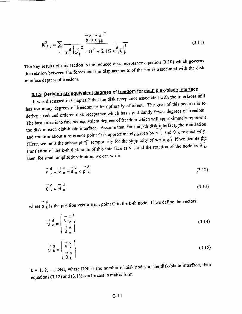
-'d -_d T

(3.11)

The key results of this section is the reduced disk receptance equation (3.10) which governs

the relation between the forces and the displacements of the nodes associated with the disk

interface degrees of freedom.

3.1.3 _ six _ _ of freedom for each _ Interface

It was discussed in Chapter 2 that the disk receptance associated with the interfaces still

has too many degrees of freedom to be optimally efficient. The goal of this section is to

derive a reduced ordered disk receptance which has significantly fewer degrees of freedom.

The basic idea is to find six equivalent degrees of freedom which will approximately represent

the disk at each disk-blade interface. Assume that, for the j-th disk interface, c_he translation

and rotation about a reference point O is approximately given by v o and 0 o respectively.

(Here, we omit the subscript "j" temporarily for the simplicity of writing.) If we denote]the

translation of the k-th disk node of this interface as v k and the rotation of the node as 0 k,

then, for small amplitude vibration, we can write

--'d -'d "-"d -'d

V k = V o+0o x Pk

--'d "-'d

0k=0o

--'dwhere p k is the position vector from point O to the k-th node. If we define the vectors

---d o

uo-t f,o

"-'d kIlk=

(3.12)

(3.13)

(3,14)

(3,15)

k = 1, 2, ..., DNI, where DNI is the number of disk nodes at the disk-blade interface, then

equations (3.12) and (3.13) can be cast in matrix form

C-11

-*d d _dU k=Qk,o o (3.16)

where

I

0

dW k,o

I

dW k,o

0

- -(;:)z

and I is the 3 by 3 identity matrix.

(3.17)

(3.18)

--d

Now, since u 13is the displacement vector for all of the disk nodes at the disk-blade

interface, we have

--'d T [ffd T ---d T -'d T]U [5 = 1 ,,.U k ,,,U DNI (3.19)

Then equations (3.16) and (3.19) imply

d d -*d_ = Qi3,o u o (3.20)

where

T d T

-- "'"Q k,oQ13,o ,o (3.21)

Without dropping the subscript "j" for the j-th disk-blade interface, equation (3.20) would be

written as

(u _t}j= (Qd ,o)j (u do)j (3.22)

Then, for all of the interfaces, equation (3.22) implies

C-12

d d_ = Q_,o_ o

(3.23)

where, with the number of blades being denoted by NB,

u_ = ua 1... _ k... 13 NB

, (d)(,)]Q_,o = diag Qda, o I ... Q_,o k ... Ql_,o NB

(3.24)

(3.25)

_.°T (;0o)T(udlT]u o = I ... k ... o NB (3.26)

°Notice here that Q 6,o is a block-diagonal matrix with diagonal blocks Q ,o k (k -- 1, ..., NB)d

Equation (3.23) gives an approximate relation between the reduced order displacements u o---d --d

and the displacements of the interracial disk nodes u 8. u o is a vector with dimension 6°NB--'d dand u _ has a dimension of 6°DNI°NB. QI3,c is a rectangular matrix with dimension

6°DNIoNB by 6°NB.

We also need to find the resultant forces and moments for the each interface. For the j-th

disk interface, the resultant force and moment about the reference point O are

(3.27)

-"d "d --"d "-"d

1;o--Z'l:k+pkX _ k

k (3.28)

--'d -'d

where 7t o is the resultant force acting on the disk at the disk interface a_ndd't o is the resultant

moment about the reference point O acting ont_e disk at the interface. 7t k is the force acting

on the k-th disk node of the j-th interface and x k is the moment acting on the k-the disk node

of the j-th interface. Notice here that the subscript "j" is temporarily omitted for simplicity in

writing. Equations (3.27) and (3.28) can be rewritten in matrix form by using the procedure

presented earlier,

I 0

wd Tk,o I

(3.29)

C-13

skew-symmetric matrix Wdk,o has been defined in equation (3.18). If we define thewhere the

vector

Ioo

(3.30)

and recognize that

f13 = 1 1 ...ltk 17 k ..._ DNI 17 DNI(3.31)

then equation (3.30) can be written as

"_d d T-'d

o = Q 13,o f 13 (3.33)

d

where Q ILc has been previously defined in equation (321). Now, using the subscript "j"

which was dropped previously, equation (3.33) would be in fact written as

T

(3.34)

Therefore, for all of the disk-blade interfaces, equation (3.34) implies

_d d T do= Ql_,o fl_(3.35)

where, with NB denoting the number of blades,

O _- ...... O (3.36)

f13 = I_ ] ... fl_ k ... f13 NB (3.37)

d

and QI3,e was defined in e_.qt_ation (3.25). Equation (3.35) governs the relation between the"*d

resultant interracial forces, f o, and the individual nodal forces, f 13, of the interracial nodes for"_d "*d

every disk interface, f o and f l_ are vectors with dimensions 6oNB and 6.DNI.NB

respectively.

C-14

3.1,4 Reduced order disk

Equation (3.10) governs the relation between the actual interactive forces and the actual

displacements of the disk nodes at the interfaces. Equations (3.23) and (3.35) describe the

relation between actual degrees of freedom and the reduced order ones. To find the relation"d -'d

between the reduced order forces f o and the reduced order displacements u o, we need to find-'d

the inverse functio_n_! for equation (3.23) and (3,35). For equation (3,2_3) d since u o is

overdetermined by u I_, it is possible to find a least square approximation ofu o such that the

error

Jl' ' -'112Error = u/3 -Ql_,o u o (3.38)

is minimized.

simple form

-'d

The least square approximation of u o can be mathematically written in a

-"d d + d

u o =Qis,o u13(3.39)

d 4-

where Q !_,o is the generalized inverse of Q_,c with the expression

)-1 d Td + d T d

QIs,o = Q_,o QIs,o Q_,o (3.40)

-'d -'d

For equation _.35), since f B is under-determined by f o, there are many ao_ssible-'d

approximations off/3 for every given f o. However, by requestingthat the norm off _ to be

minimized, it is possible for us to find a unique approximation off I_ that retains the non-self-

equilibrated forces only and neglects the self-equilibrated forces. The expression for the non-

self-equilibrated approximation is

--d [--d +l T d

(3.41)

d +

where Q 13,o is defined in equation (3.40).

Here we are actually proposing an assumption that the self-equilibrated forces at the

interfaces are negligible. This assumption should be valid for the lower system modes since

the disk does not locally deform very much in these cases. It, however, may not be

C-15

Combining equations (3.10), (3.39), and (3.41), we can have the following equation

;d o = Rdo,o _do

where

(3.42)

and

-*d -'d T

R d _ _ j.o ¢_j.o

J mj -_ +2i_

(3.43)

"-'d d +_d¢ j,o = Q _,o j,13 (3.44)

d

R o,¢ is the reduced order _sk receptance matrix associated with the disk interfaces and has

dimension 6*NB by 6,NB. ¢ j,c is the reduced order interracial displacements for the j-th disk

mode. Equation (3.42) is the reduced order disk rec_ptance equation which governs.,dthe

relation between the reduced order displacements u o and the reduced order forces f o.

Remember that this equation is the reduced order form of equation (3.10), the disk receptance

equation associated with the disk-blade interfaces. Based on the assumption that the self-

equilibrated forces at the interfaces are negligible, equation (3.42) approximates the disk

behavior by 6 degrees of freedom per interface.

3.2 Formulation for the Blades

3.2.1 BP,,..C.IIRII!E_ formulation for a _ blade

To begin with, let us consider a single blade which is clamped at its base. The blade base

moves rigidly so that its motion can be fully described by 6 degrees of freedom, namely, 3-'b

translations and 3 rotations. Let x o be the 6-degree-of-freedom displacement vector of the

blade base, where O is a reference point residing at the blade base. Using subscript "9" to

denote the group of blade nodes which reside at the blade base and subscript "or" to denote

the nodes other than the nodes of group 13,the equations of motion for the entire blade can be

written as

C-16

ct,ct Za + ,a a + ,ctZa =fct e

_big2t _ M b b

Ix,or Qot,O X 0 (3.45)

--*b "--b b --'bx(z "--Zo C + _,/a,o x o (3.46)

-'b Qb --'bx 13= ,o x o (3.47)

ba Cbot bK'ba mass, damping, and stiffness matrices associated withwhere M ,a, ,a, and ,a ar_,ethe b -- b

the group-ct nodes, x a and x 13 are the displacements of the blade. Qct,oX o is the

displacement vector of the group-a nodes assuming that the blade follows the base and does-'b

not deform at all. b z ct is the deformation of the group-ct nodes relative to the unde_ormedconfiguration, f ct e int is the external force acting on the blade. M b ba,ctQa,o x o is an

inertial force associated with the blade base motion that is introduced when writing the

equations of motion in terms of relative motion. The derivations of matrices Q_,o and Q°_, o

t_ t_

are similar to the process described in Section 3.1.3; we will not repeat it here. When the

bladed disk is operated at a stationer)' speed, the steady-state response of the blade can be

written as

---b -- b if_tXot =Ua e

(3.48)

--" b "* b ifltx13 =Ul_ e (3.49)

b _ b i_tXo=Uoe

(3.50)

Substituting equations (3.48), (3.49), and (3.50) back into equations (3.45), (3.46), and (3.47)

and eliminating time-dependent terms, we have

b Rb "b { ) b -'bua = a,af a + _2 Rba,ct Mba,a +I Qa,o u o(3.51)

-'b b -'bul3=Ql_,oUo (3.52)

where Rba,ct is the receptance matrix associated with the group-a nodes, It has the expression

C-17

.b (< _°2M )-'a,= = ,c_ a,u + i ft C-'ba,a (3.53)

_s discussed in Section 3.1.1. calculating the inverse of the dynamic impedance matrix

Ilia,a_ f_2 M_,a + i f_ cba,a)is undesirable since the matrix tends to be ill-conditioned

when the excitation frequency f2 is close to the natural frequencies of the blade. Similar to the

way we formulate the receptance equation for the disk, the receptance R ba,a can be cast in the

following form by applying the standard modal analysis technique,

"b -"b T

Rb ¢ j,a ¢ j,al (3.54)

J mt_to3_ 2- f_2+2it2 4 _1

--b bwhere ¢ j,ais thej-th mode for a blade clamped at its base, and mi_, _ , and mj are the modal

mass, modal damping ratio, and natural frequency of the j-th mode. It should be empha_z_d

that the degrees of freedom of the group-13 nodes do not appear in equation (3.54) since _ j,13,

the mode shapes at the blade's base, are zero.

Force on the blaOe tmse

While equations (3.51)band (3.52) enable us to calculate_b the motion of the blade for any

given external excitation f a and blade base motion u o, we have not yet determined the"b

resultant force on the blade base. The resultant force on the blade base, denoted as f o

hereafter, needs to be known in order to assemble the equations for the disk-blade interfaces.

To achieve this, we first consider the blade as an object which can move and deform in space."b

The forces acting on the blade are the excitation force f a and the interactive force at the blade"b

interface f o. Since the linear momentum and angular momentum have to be conserved, we can

write the conservation law, about the reference point O, for small amplitude vibrations,

-:.b -"b

ZLk=Z_ke

k k

it'/t

(3.55)

Z k+P kxLk= k+pkX_ e

k k

iflt

(3.56)

"b --'b

where L k is the linear momentu_obfthe k-_bhblade node, H k is the angular momentum of the

k-th node about the node itself, n k and x k are the force and the moment acting on the k-th

C-18

-'bblade node, and p k is the position vector from the reference point O to the k-th node.

defining the following 2 vectors,

By

.bT- T T1P = 1 1 ""Lk Hk ...LBN HBN(3.57)

[_bT_b T --'bT-*b T _b T-*b T]_T= 1 1 ""_k l:k ". 7tBN 'tBN(3.58)

where BN is the number of blade nodes, equations (3.55) and (3.56) can be rewritten in matrix

form,

b T • b b TQoP = Qo _b e int

(3.59)

where Qb o is a 6_BN by 6 matrix which can be derived by the same procedure presented inb

Section 3.1. Q o has the function of calculating the resultant momentum about the reference

point O.

Now, by definition, the momentum of the blade can be written as

--b ._bp =Mbx

(360)

where M b is the mass matrix of the entire blade. For the steady-state vibration,

-" b "" b iQt

X = U e (3.61)

Substituting equations (3.60) and (3.61) into equation (3.59) and eliminating the time-

dependent terms, we have

b T b T_f_EQo Mbub=Qo _b

(3.62)

Recall that equations (3.51) and (3,52) describe the displacements of the blade nodes. By

substituting them into equation (3.62) and recognizing that

b b T"bo = QI3,o fl_ (3.63)

C-19

we have

_b z_ u b b-bo- o,o o+Hot_ f(3.64)

where

b T b TZboo __2 Qo Mb b _4 M b R b M b b. = qo- Qa,o a._ a._ _.- Qa,o (3.65)

H b __2 b T Mb R b b Toa = Qa,o a,a a,a -Qa,o (3.66)

-*b

Equation (3.64) gives the expression of f o, the interactive force a_il_g on the blade base, in"-'bterms of the blade base displacement u o and the external excitation f a. The calculation of the

coefficient matrices Zbo ( and H b, oft are tedious but straight forward. Notice again that the

blade receptance R b will be calculated using the blade modes (equation (3.54)) instead ofO_,a

directly finding the inverse of the dynamic impedance (equation (3.53)). This remark is

important since equation (3.54) is efficient and stable when implemented computationally.

Formulation for all

Equation (3.64) is written for the j-th blade Including the subscript "j", it should be

written as

Therefore, for all of the blades, the equation that governs the states of the blade bases is

where

o = o,o o+H afa

• bTlbT[( I ( ) ].-.- b T

U o = Ho 1"" Ho j "'" Ho NB

fa = f_ l""lfa)j "'" f NB

(3.66)

(3.67)

(3.68)

(3.69)

(3.70)

C-20

b

IHbo,alj,j= I,2, ...,NB, respectively.

3.3 Assembling Disk and Blades

Recall that the purpose of the analysis is to develop a computationally efficient algorithm

to solve for the steady-state vibration of the blades. Equations (.3651) and (3.52) enable us to

calculate the blade vibration provided that the external excitation f _xand the blade base motion---b

u o are given. Since the external excitation is usually given, our goal is to solve for the blade

base motions.

While equation (3.42) governs the motion of the disk nodes residing at the disk-blade

interfaces, equation (3.67) governs the motion of the blade..,d--dn°deS--bresidin_ at the disk-blade

interfaces. Since there are 4 unknown vectors, namely, u o, f o, u o, and f o in the equations

We need to introduce two additional equations to govern the behavior of the disk-blade

interfaces. The first of these is Newton's Interactive Force Law which conserves momentum

at the interfaces,

(3.73)

The second is Hooke's Law which provides a constitutive relation at the interfaces,

0 "-- K o,o o-(3.74)

where K o,t is a matrix which represents the stiffness of the disk-blade attachments. Since the

attachment stiffness is in general determined by separate analyses, we will consider it as a

known quantity. By solving equations (3.42), (3.67), (3.73), and (3.74) simultaneously, we

-bcan express the 4 unknowns in terms of the external excitation f a

C-21

u_o--(.'o,o+KoljEI+eo,o(._o,o+KoI_-I Hbo_ _ b'_ (3.75)

"b I (R d -111-1 b -'bf o = I + Zbo,o o,o + K o, H oxt f a (3.76)

;_ -¢5,+ eoo(¢o.o+,,-:.l]-_,Coo_o = , ct (3.77)

[ (Rdo,o+K_ll]-I bo -'bdo = - I + Zbo,o o, H _t f a (3.78)

Recall that, equations (3.51) and (3.52) express the blade vibration in terms of the external

excitation and the blade base motion. Therefore, the vibrations of the blades can be easily

derived by substituting equation (3.75) into equations (3.51) and (3.52).

It is important to notice that the most_computationally intensive part in equations (3.75)

L (_ -'11is to calculate the inverse of the matrix | + Zbo,o R o,o + K o, • The dimension of this

matrix is 6°NB by 6.NB which is significantly smaller than the dimension of a general finite

element model of a bladed disk. For a typical bladed disk with, for instance, 65 blades, the

finite element model could have thousands of degrees of freedom to be solved for; however,

the number of the unknown degrees of freedom is only 390 (= 6-65) if we use the reduced

order model.

Chapter 4: COMPARISON OF RESULTS

In Chapter 3, we have developed the algorithm for the reduced order modeling to solve for

the forced vibration of bladed disks. In this chapter, the algorithm will be tested on a

simplified model problem. A code named LMCC (Linear Mistuning Computer Code) has

been developed based on the algorithm. The results of LMCC will be compared with the

results of the direct finite element approach to examine the validity of the reduced order

model.

C-22

4.1 Attachment Stiffness and Damping Ratios

Before we implement the proposed algorithm, there are still several parameters of the

reduced order model left to be determined. The first is the attachment stiffness matrix K o,<

which simulates the stiffness of the disk-blade attachments (see equation (3.74)). Because of

the simplified geometry of our test problem, the attachment stiffness is effectively infinite.

Equation (3.74) then implies the continuity in displacements

(4.1)

and equations (3.75), (3.76), (3.77), and (3.78) become

;b Rdoo [ o,oRdo,l-1 bo --bo =- , I +Z b H _fa(4.2)

-'b [ Rd 1-i b -'bfo = I +Zbo,o o, Ho_ fa(4.3)

u d _Rdo,o[ Rd I -1 b° --bo = I +Zbo,o o. H _ fa(4.4)

_d [ Rd 1-1 bo --b°=--I +Zbo,o o, H x_fQ(4.5)

The other parameters of the reduced order model to be determined are the damping ratios

of the substructures' modes. Since the mechanism of the structural damping is not well-

realized so far, it is difficult to accurately determine these damping ratios by analytical

methods. However, since the peak amplitude of a slightly damped system is proportional to

the reciprocal of its damping ratios, we are able to determine these damping ratios by

numerical experiments. The procedure was used is the following:

l, Assume the damping ratios of the substructures' modes are equal to some small value.

A better choice is the damping ratios of the system modes (if they are available)

because, based on our experience, the damping ratios of the substructures' modes are

in general approximately equal to those of the system modes.

. Adjust the damping ratios of the substructures' modes such that the peak amplitude of

the tuned response of the reduced order model matches that of a reliable source, for

example, the physical experiment.

C-23

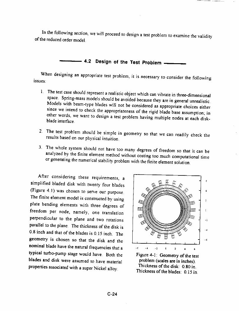
In the following section, we will proceed to design a test problem to examine the validity

of the reduced order model.

4.2 Design of the Test Problem

When designing an appropriate test problem, it is necessary to consider the following

issues:

, The test case should represent a realistic object which can vibrate in three-dimensional

space. Spring-mass models should be avoided because they are in general unrealistic.

Models with beam-type blades will not be considered as appropriate choices either

since we intend to check the appropriateness of the rigid blade base assumption; in

other words, we want to design a test problem having multiple nodes at each disk-

blade interface.

2. The test problem should be simple in geometry so that we can readily check the

results based on our physical intuition.

. The whole system should not have too many degrees of freedom so that it can be

analyzed by the finite element method without costing too much computational time

or generating the numerical stability problem with the finite element solution.

After considering these requirements, a

simplified bladed disk with twenty four blades

(Figure 4.1) was chosen to serve our purpose.

The finite element model is constructed by using

plate bending elements with three degrees of

freedom per node, namely, one translation

perpendicular to the plane and two rotations

parallel to the plane. The thickness of the disk is

0.8 inch and that of the blades is 0.15 inch. The

geometry is chosen so that the disk and the

nominal blade have the natural frequencies that a

typical turbo-pump stage would have. Both the

blades and disk were assumed to have material

properties associated with a super Nickel alloy.

4

C

I

Figure 4-1: Geometry of the test

problem (scales are in inches).Thickness of the disk: 0.80 in.

Thickness of the blades: 0.15 in.

C-24

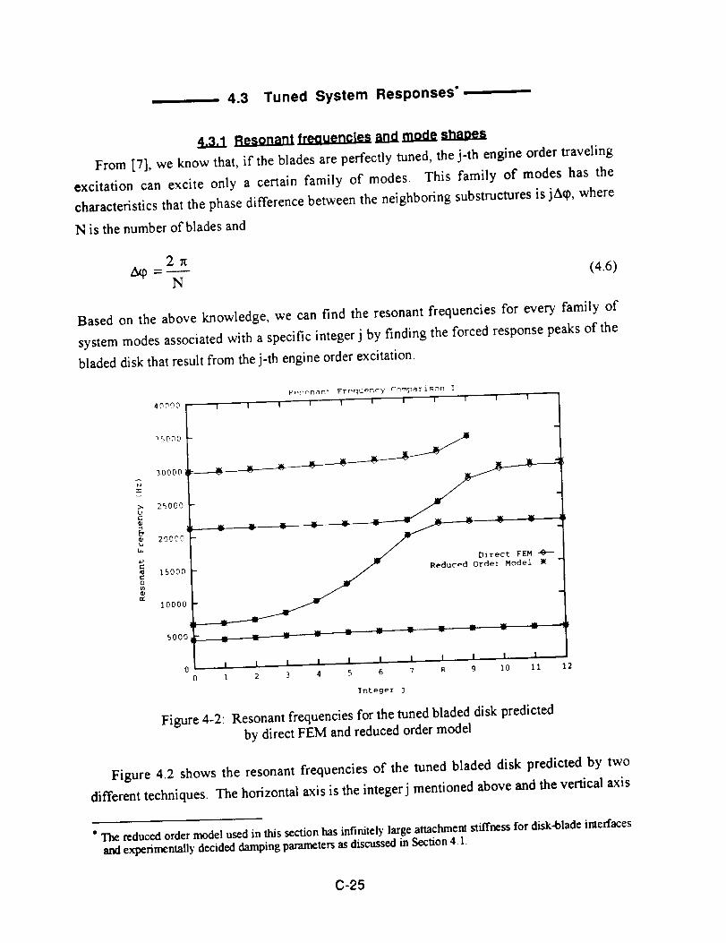
4.3 Tuned System Responses"

Resonant _ and mode _J_._.S

From [7], we know that, if the blades are perfectly tuned, the j-th engine order traveling

excitation can excite only a certain family of modes. This family of modes has the

characteristics that the phase difference between the neighboring substructures is jar0, where

N is the number of blades and

27t

Aq)=_N (4.6)

Based on the above knowledge, we can find the resonant frequencies for every family of

system modes associated with a specific integer j by finding the forced response peaks of the

bladed disk that result from the j-th engine order excitation.

N"V"

L)c'

L,.

o

P_*r_na_' Frequency C_mpari_n

40@_0 I I I I I l

_ooo

30000

25000

20000

15000

I0000

5000

I I 1 1 I

I I I I I I 1 I I I I

1 2 3 4 5 6 7 _ 9 i0 II

Integer j

Figure 4-2: Resonant frequencies for the tuned bladed disk predicted

by direct FEM and reduced order model

12

Figure 4.2 shows the resonant frequencies of the tuned bladed disk predicted by two

different techniques. The horizontal axis is the integer j mentioned above and the vertical axis

* The reduced order model used in this section has infinitely large anachmenl _iffness for disk-blade interfacesand experimentally decided damping parameters as discussed in Section 4.1.

C-25

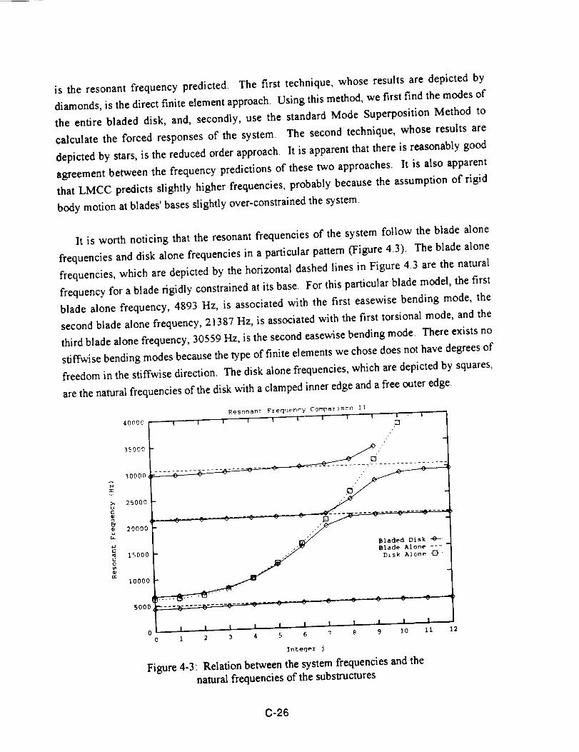
is the resonant frequency predicted. The first technique, whose results are depicted by

diamonds, is the direct finite element approach. Using this method, we first find the modes of

the entire bladed disk, and, secondly, use the standard Mode Superposition Method to

calculate the forced responses of the system. The second technique, whose results are

depicted by stars, is the reduced order approach. It is apparent that there is reasonably good

agreement between the frequency predictions of these two approaches. It is also apparent

that LMCC predicts slightly higher frequencies, probably because the assumption of rigid

body motion at blades' bases slightly over-constrained the system.

It is worth noticing that the resonant frequencies of the system follow the blade alone

frequencies and disk alone frequencies in a particular pattern (Figure 4.3). The blade alone

frequencies, which are depicted by the horizontal dashed lines in Figure 4.3 are the natural

frequency for a blade rigidly constrained at its base. For this particular blade model, the first

blade alone frequency, 4893 Hz, is associated with the first easewise bending mode, the

second blade alone frequency, 21387 Hz, is associated with the first torsional mode, and the

third blade alone frequency, 30559 Hz, is the second easewise bending mode. There exists no

stiffwise bending modes because the type of finite elements we chose does not have degrees of

freedom in the stiffwise direction. The disk alone frequencies, which are depicted by squares,

are the natural frequencies of the disk with a clamped inner edge and a free outer edge.

AN,r

_wt_

r"

orr

40090

35000

30000

25000

20000

15000

10000

5000

R_sonant Frequenry Comparigon II

| I I I I I I I ! I ,-- 1

U

._____,._v ___________ __-¢_____ v_--- _ /_. .... _ ....... _ .... _ ....

Bladed DiskBlade Alone ---Disk Alone 4_}-

_--- _- .... _-----_ .... -_-.... _ .... _ _- _ _ - _

0 f m m J ! ! f I l I I1 2 3 4 5 6 "7 8 9 10 11

Integer j

Figure 4-3' Relation between the system frequencies and the

natural frequencies of the substructures

12

C-26

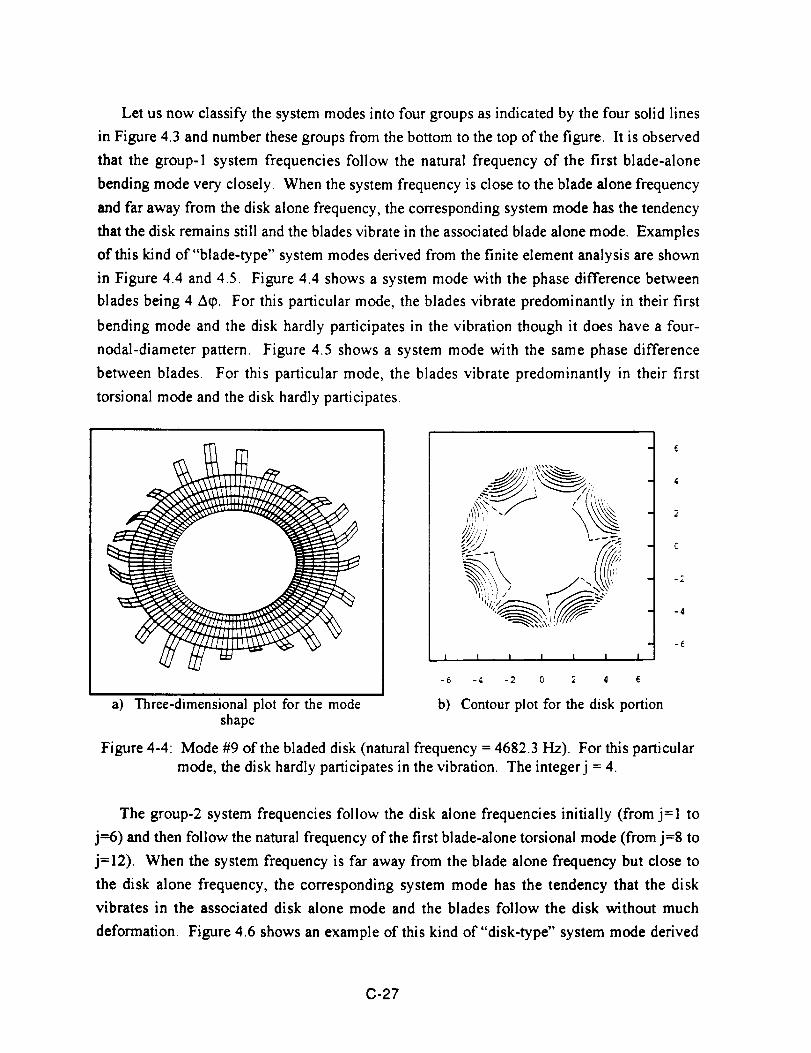
Let us now classify the system modes into four groups as indicated by the four solid lines

in Figure 4.3 and number these groups from the bottom to the top of the figure. It is observed

that the group-1 system frequencies follow the natural frequency of the first blade-alone

bending mode very closely. When the system frequency is close to the blade alone frequency

and far away from the disk alone frequency, the corresponding system mode has the tendency

that the disk remains still and the blades vibrate in the associated blade alone mode. Examples

of this kind of "blade-type" system modes derived from the finite element analysis are shown

in Figure 4.4 and 4.5. Figure 4.4 shows a system mode with the phase difference between

blades being 4 Acp. For this particular mode, the blades vibrate predominantly in their first

bending mode and the disk hardly participates in the vibration though it does have a four-

nodal-diameter pattern. Figure 4.5 shows a system mode with the same phase difference

between blades. For this particular mode, the blades vibrate predominantly in their first

torsional mode and the disk hardly participates.

a) Three-dimensional plot for the modeshape

K_..........._j, _,,,,,,,,

--- \\% -fTY -

<

I I I I I I I

-6 -4 -2 0 2 4 6

b) Contour plot for the disk portion

6

4

2

C

-Z

-4

-£

Figure 4-4: Mode #9 of the bladed disk (natural frequency = 4682.3 Hz). For this particular

mode, the disk hardly participates in the vibration. The integerj = 4.

The group-2 system frequencies follow the disk alone frequencies initially (from j=l to

j=6) and then follow the natural frequency of the first blade-alone torsional mode (from j=8 to

j=12). When the system frequency is far away from the blade alone frequency but close to

the disk alone frequency, the corresponding system mode has the tendency that the disk

vibrates in the associated disk alone mode and the blades follow the disk without much

deformation. Figure 4.6 shows an example of this kind of "disk-type" system mode derived

C-27

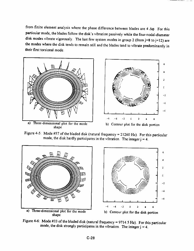
from finite element analysis where the phase difference between blades are 4 Atp. For this

particular mode, the blades follow the disk's vibration passively while the four-nodal-diameter

disk modes vibrate vigorously. The last few system modes in group 2 (from j=8 toj=12) are

the modes where the disk tends to remain still and the blades tend to vibrate predominantly in

their first torsional mode.

I 1 I I 1 i

-6 -4 -2 0 2 4 6

6

4

2

C

-2

-4

-f.



Figure 4-5: Mode #57 of the bladed disk (natural frequency = 21260 Hz). For this particular

mode, the disk hardly participates in the vibration. The integerj = 4.


Figure 4-6:

I

-6

b)

I I 1 I I 1 _

-4 -,2 0 2 4 6

Contour plot for the disk portion

6

4

2

-4

-6

Mode #33 of the bladed disk (natural frequency = 9714.5 Hz). For this particular

mode, the disk strongly participates in the vibration. The integerj = 4.

C-28

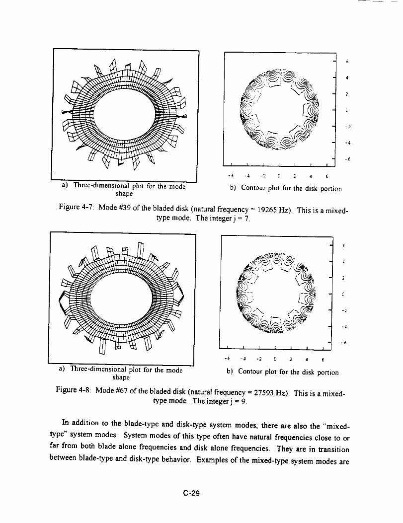
I

-6

,,/_!_>'I _,_;_ ,

I I I 1 I I

-4 -2 0 2 4 E

6

4

2

[

-2

-4

-E



Figure 4-7: Mode #39 of the bladed disk (natural frequency = 19265 Hz). This is a mixed-

type mode. The integer j = 7.

>


-%

,, -_ _ -2

-6

1 I I I I I 1

-_ -4 -2 0 2 4 6


Figure 4-8: Mode #67 of the bladed disk (natural frequency = 27593 Hz). This is a mixed-

type mode. The integer j = 9.

In addition to the blade-type and disk-type system modes, there are also the "mixed-

type" system modes. System modes of this type often have natural frequencies close to or

far from both blade alone frequencies and disk alone frequencies. They are in transition

between blade-type and disk-type behavior. Examples of the mixed-type system modes are

C-29

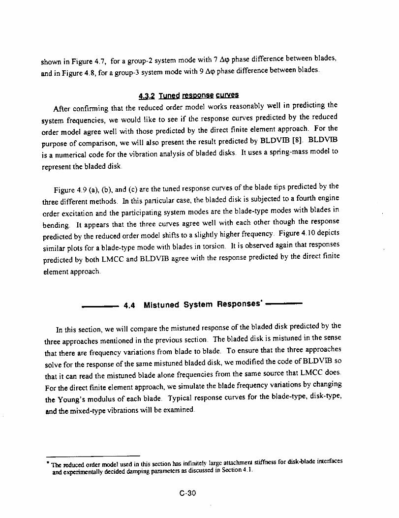
shown in Figure 4.7, for a group-2 system mode with 7 Aq> phase difference between blades,

and in Figure 4.8, for a group-3 system mode with 9 Aq_ phase difference between blades.

4,3,2 Tuned _ cu_es

After confirming that the reduced order model works reasonably well in predicting the

system frequencies, we would like to see if the response curves predicted by the reduced

order model agree well with those predicted by the direct finite element approach. For the

purpose of comparison, we will also present the result predicted by BLDVIB [8]. BLDVIB

is a numerical code for the vibration analysis of bladed disks. It uses a spring-mass model to

represent the bladed disk.

Figure 4.9 (a), (b), and (c) are the tuned response curves of the blade tips predicted by the

three different methods. In this particular case, the bladed disk is subjected to a fourth engine

order excitation and the participating system modes are the blade-type modes with blades in

bending. It appears that the three curves agree well with each other though the response

predicted by the reduced order model shifts to a slightly higher frequency. Figure 4.10 depicts

similar plots for a blade-type mode with blades in torsion. It is observed again that responses

predicted by both LMCC and BLDVIB agree with the response predicted by the direct finite

element approach.

4.4 Mistuned System Responses"

In this section, we will compare the mistuned response of the bladed disk predicted by the

three approaches mentioned in the previous section. The bladed disk is mistuned in the sense

that there are frequency variations from blade to blade. To ensure that the three approaches

solve for the response of the same mistuned bladed disk, we modified the code of BLDVIB so

that it can read the mistuned blade alone frequencies from the same source that LMCC does.

For the direct finite element approach, we simulate the blade frequency variations by changing

the Young's modulus of each blade. Typical response curves for the blade-type, disk-type,

and the mixed-type vibrations will be examined.

"The reduced order model used in this section has infinitely large attachment stiffness for disk-blade interfacesand experimentally decided damping parameters as discussed in Section 4.1.

C-30

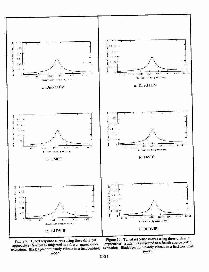
¢_ C C5

CC3

C _:

T-

r :(

__ c :s

: :_

C Z(

E C C.=

C :4

==- COl

o

I, , ,45!: 4_:1 4_: 4::C 4"5: (EC:

a. Direct FEM

I 1 1 I 1|

4_ : : 4_. =-: 4": : 4-. r : 4_: : 4E5:

b. LMCC

I' I i i I 'I ' ]

I--

4E_: 46C: 4F._C 4"_CC 4"T5C 48DC

c. BLDVIB

C G:2

b

C_C2

C CC]

Z D:_

C :::

: :::_

c

C C:;5

¢ C C:_

CCC;

C CC:_

I I I I 1 I I

, I l I I I I

a. Direct FEM

t I I l I i l

b. LMCC

I I I I i I I ' '=

_xc_tl_iOn _e_l_Jency {NZ)

c. BLDVIB

Figure 9: Tuned response curves using three different Figure I0: Tuned response curves using three differentapproaches. System is subjected to a fourth engine order approaches. System is subjected to a fourth engine order

excitation. Blades predominantly vibrate in a first bending excitation. Blades predominantly vibrate in a first torsionalmode. mode.

C-31

I_.Jfl.CP,.:IgO_ system vibration

Figure 4.11 (a), (b), and (c) are the typical mistuned response curves of the blade tips

predicted by the three different approaches. In this case, the bladed disk is subjected to a

fourth engine order excitation and the participating system modes are basically the blade-type

modes with blades in bending. The tuned response induced by the same excitation was

discussed in the previous section (Figure 4.9). It appears that the reduced order model and the

spring-mass model give equally good results.

Figure 4.12 shows the mistuned response curves of the blade tips predicted by the three

different approaches. In this case, the bladed disk is subjected to a fourth engine order

excitation and the participating system modes are the blade-type modes with blades in

torsion. The response of the tuned stage was discussed in the previous section (Figure 4.10).

We can see that LMCC works much better than BLDVIB, though they predict equally well

the results for the tuned stage. One of the possible explanation for the failure of BLDVIB in

this particular case is that the spring-mass model does not account for the effects of three-

dimensional motion and multiple node attachment at the disk-blade interfaces. By observing

Figure 4.12(c), we also find that the blades do not interact as much as they should. This leads

to another possible reason for the failure of the spring-mass model that they can not account

for the complicated blade-to-blade coupling effect while the blades vibrate predominantly in

their first torsional mode.

4.4.2 _ system vibration

Figure 4.13 shows the comparison of the mistuned results predicted by the direct finite

element approach and the reduced order model. For this particular case, the bladed disk is

subjected to a fourth engine order excitation and the disk participates vigorously in the

vibration since the natural frequency of the four-nodal-diameter disk modes is very close to

the system frequency. It appears the result predicted by the reduced order model agrees well

with the result predicted by the direct finite element approach. It is interesting to observe

that the blade mistuning does not affect the disk-type vibration very much.

4.4.3 t_LEC.:.tY.Rt system vibration

Figure 4.14 and Figure 4.15 are the mistuned responses for the mixed-type system

vibration. The vibration is mixed in the sense that both the disk and the blades participate in

the vibration and it is hard to tell which blade alone mode the blades vibrate in. Figure 4.14

shows the response curves for the mistuned bladed disk under a seventh engine order

excitation. Figure 4.15 shows the response curves for a mistuned bladed disk under a ninth

C-32

(.-

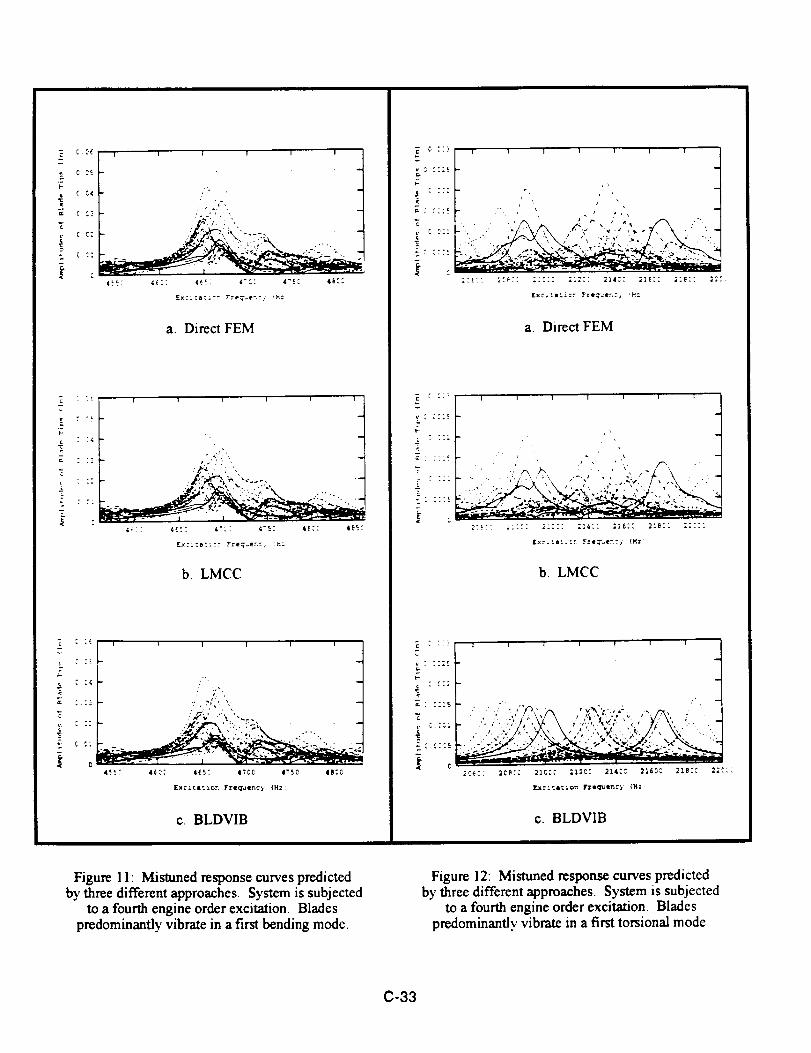
i

tT-

7

r

C O(

C CE

C _,4

c ".3

C C;

I I I I I I

):- .

a. Direct FEM

7. t

: :2

I 1 I I I 1

.u

:/7,

r;,P-_

b. LMCC

C C"

0

I I I I I I i

.._, ,'%.._,2_ " 1

Exc;titlor, Fre_incy IH::

c. BLDVIB

C 773

: :33

u : :::£

I-

I I I I I I I

a. Direct FEM

I I I I i i i

k

• "' " "J -\' _\ ,"-'_ " ' .I;,¢ __ \ ' ." "

b. LMCC

I I I I t I i

.. ,.., \ ,',!;,,,:<,.,..,'x;"'t,>.." ,. ,:..'A. 'A, \, ,e..., V..,'.','_.//, _< -....

" .'"..,,'<", _. ,...., ,,,: ,....,. ,, .....,,_: : 2D[:: : _15_C _12C_ 214_: 2169_ 2IB:: 2;:::

F.xCltit1On Fie(ill,line)' (Hi

c. BLDVIB

Figure 11: Mistimed response curves predictedby three different approaches. System is subjected

to a fourth engine order excitation. Bladespredominantly vibrate in a first bending mode.

Figure 12: Mistuned response curves predictedby three different approaches. System is subjected

to a fourth engine order excitation. Bladespredominantly vibrate in a first torsional mode.

C-33

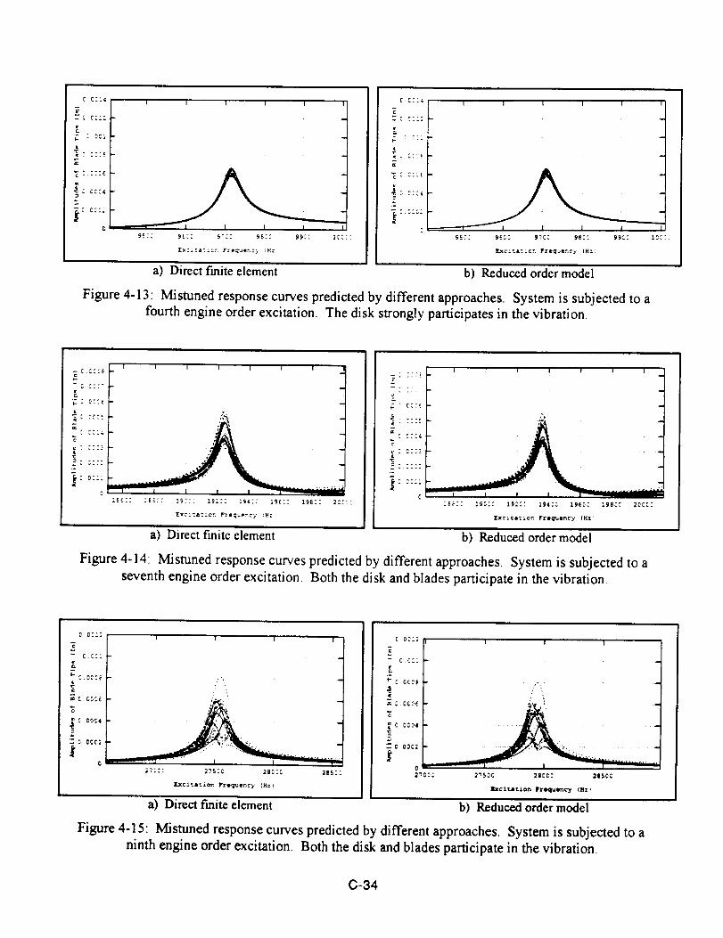
C C::4

E: oc.:

p.

te

_c c::4

t I I I I |

I I I I

Ex:._ta:.;::-. Freq'._er.=,, rH:

a) Direct finite element

IICC::

C C::_

= C C::=

: CZI

¢

v

; CCC¢

C CCC;

I I I I I

, I J i9EZC 9{C6 9_CC 98:C 99:7

E.xc:tl:;cr. Fre_e,":,=_ {Mz

ICC71

b) Reduced order model

Figure 4-13: Mistuned response curves predicted by different approaches. System is subjected to a

fourth engine order excitation. The disk strongly participates in the vibration.

C :::E

C :C: t.

r OCC;

=E(.'I =EEZ: 19Z'Z 19;CC 194:Z 19(:: IgECC 2CC-'Z

Ex:==a=:.cr, Frec_ue,-.cy '_H:

Z CZZ_

C CZ:-

.... c

C

I I I I I I /

"1

1_-2 Z 19C'-" 192:: 194C; 19ECC 198:C _OCC:

EX:_ta:iC_ Fze_r_eney {MI I

a) Direct finite element b) Reduced order model


seventh engine order excitation. Both the disk and blades participate in the vibration.

i C.O_C_ - ,,,., , ./

C 0004 .....

o_m--_ , _l,, I .....

27CCZ

I

27500 2BCGC

hCi_ItiO_ F_(_rUl_Cy [H=_

_05::

C OC:;

-- C CC:

P C CC:_

{

C OD04

= C.O00_

0

I I I _J

2 %,

Ill'I:

2750C 210O_ 2ll_OC

aP,,¢itat_on _r_lnc_ (Mz)

a) Direct f'mite element b) Reduced order model


ninth engine order excitation. Both the disk and blades participate in the vibration.

C-34

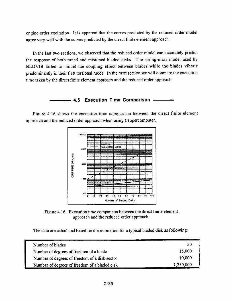
engine order excitation. It is apparent that the curves predicted by the reduced order model

agree very well with the curves predicted by the direct finite element approach.

In the last two sections, we observed that the reduced order model can accurately predict

the response of both tuned and mistuned bladed disks. The spring-mass model used by

BLDVIB failed to model the coupling effect between blades while the blades vibrate

predominantly in their first torsional mode. In the next section we will compare the execution

time taken by the direct finite element approach and the reduced order approach.

4.5 Execution Time Comparison

Figure 4.16 shows the execution time comparison between the direct finite element

approach and the reduced order approach when using a supercomputer.

i-

1W

B _Or_ M_ciJ i i

........ !.

........... i-_''2, - -_- i i- i ---

.I . i : e .:

; " t ..... i"" |

' : i : [ i

.; .... ;' ........0 10 20 30 40 SO 60 70 80 90 100

Number of Bladed Disks

Figure 4.16: Execution time comparison between the direct finite element

approach and the reduced order approach.

The data are calculated based on the estimation for a typical bladed disk as following:

Number of blades

Number of degrees of freedom of a blade

Number of degrees of freedom of a disk sector

Number of de_;rees of freedom of a bladed disk

5O

15,000

10,000

1,250,000

C-35

The estimated CPU time for solving for 100 system modes is 1,000 CPU minutes per bladed

disk. The time for calculating the forced response using Mode Superposition Methods is

approximate 0.02 minute for every 100 excitation frequencies. Therefore, we can write down

the following equation for the relation between the execution time needed by using the direct

finite element approach and the number of bladed disks analyzed,

T fern = 1000.02 N (4.7)

where N is the number ofbladed disks.

If we use the reduced order approach for the blade mistuning problem, the CPU time for

solving for the modes of a nominal blade is approximate 15 minutes and that for the disk

modes is approximate 250 minutes provided that the cyclic symmetric boundary conditions

are used to improve the computational efficiency. The CPU time needed to process the

output of the finite element analysis for the use of LMCC is approximate 15 minutes. And,

for every 100 excitation frequencies, LMCC will take approximate 5 minutes to calculate the

forced response. Therefore, we can write down the equation for the relation between the

execution time needed by using the reduced order approach and the number of bladed disks

analyzed,

T lmcc = 280 + 5 N (4.8)

An immediate comparison we can obtain from observing equations (4.7) and (4.8) is that, for

every additional bladed disk, the direct finite element approach needs 1000 more minutes but

LMCC (the reduced order approach) needs only 5 more minutes. Figure 4.16 shows that, for

a typical mistuning analysis with 100 bladed disks analyzed, the direct finite element

approach needs 100,002 minutes and the reduced order approach needs only 780 minutes.

Chapter 5: CONCLUSIONS AND SUGGESTIONSIIII

5.1 Conclusions

Mistuned vibration of bladed disks has drawn much attention since it can result in large

blade-to-blade amplitude variations and the high response blades can fail from high cycle

C-36

fatigue. Due to the severe operating conditions that modem aircraft are subjected to, accurate

predictions of the vibration ofmistuned bladed disks become necessary. Using finite elements

to model a bladed disk is not a feasible approach for a thorough mistuning analysis since the

geometry of a bladed disk is so complex that a structurally accurate finite element model

would have too many degrees of freedom. Using spring-mass models to represent a bladed

disk results in low degree-of-freedom formulations. Though they can be efficiently and

reliably solved by computers, the ad hoc way in which they choose system parameters and

their questionable accuracy are undesirable.

To develop a structurally accurate and computationally efficient model for the bladed

disks, we first considered the receptance method. Though the receptance method can

significantly reduce the number of degrees of freedom of the system, the resultant equations

can still have too many degrees of freedom since the disk and the blade usually contact at

multiple points. Its necessity of using free-free blade modes is especially undesirable since, in

general, blades tend to vibrate like clamped-free modes and much of the work done on the

blades utilizes cantilever blades.

The reduced order modeling follows the idea of the receptance method but further

assumes that the blade bases undergo rigid body motion. The blade vibration is considered as

a combination of blade base motion and cantilever blade modes. By finding the six equivalent

degrees of freedom for the disk vibration at each disk-blade interface, we are able to reduce the

number of degrees of freedom of the whole structure down to six times the number of blades.

With this significant reduction in the number of unknowns, the reduced order model results in

a formulation that can be efficiently solved by computers. Along with its low computational

cost, the reduced order model is structurally accurate and provides a straight forward

approach for modeling the system since it directly takes the results from the finite element

analysis of a tuned system without ad hoc assumptions.

The validity of the reduced order model was examined by applying its algorithm to solve

for the forced response of a carefully designed test problem. The test problem is designed so

that it represents a realistic object that vibrates in three-dimensional space and has multiple

nodes at each disk-blade interface. For the purpose of comparing the reduced order model

with other reliable techniques, the geometry of the test problem is relatively simple so that it

can be efficiently solved by the direct finite element approach. It is shown in Chapter 4 that

the reduced order model can predict the tuned system frequencies reasonably well. By

comparing the results from the different approaches, it appears that the reduced order model

C-37

is able to capture the characteristics of the mistuned bladed disk. It predicted response curves

that are almost identical to the results of the direct finite element approach for the more than

one hundred cases examined, of which the cases presented in Chapter 4 were representative.

The results predicted by a typical spring-mass model are also examined. It appears that the

spring-mass model predicts mistuned responses well when the blades vibrate in bending

modes but predicts poorly when the blades vibrate in high frequency torsional modes.

Based on the investigations we have done, we can conclude that the reduced order model

is a valuable model for the vibration analysis of mistuned bladed disks. It is valuable for the

following reasons:

. It is structurally accurate and can be used for bladed disks of various kinds of

geometry because it utilizes the output of general finite element models instead of

being restricted to springs and masses or plates and beams.

. It is straight forward in the sense of modeling since the system parameters are directly

taken from the output of the finite element analysis instead of making ad hoc

assumptions.

. It is computationally efficient because the number of degrees of freedom of its

formulation is only six times the number of blades. This number is significantly

smaller than that of a finite element model and of the same order of that of a more

complicated spring-mass model, for example, [9].

5.2 Suggestions

One of the subjects of bladed disk vibration under intensive study nowadays is the friction

related mistuning problem. Blade-to-blade and blade-to-ground friction dampers are integrated

into the bladed disk assemblies to dissipate energy so that the peak amplitudes of blade

vibration can be reduced. Since the nonlinear friction forces are sensitive to the displacements

and, sometimes, to the velocities of the blades, it is necessary for the analysts to have a

structurally accurate model. Much of the work has been done on this subject is based on

spring-mass models. With proper tuning, spring-mass models often predict reasonably

accurate responses for a linear system; however, their ability in predicting the response of a

nonlinear system is questionable since friction forces can considerably change the mode

shapes of the blades and this change can hardly be modeled by simple spring-mass systems.

C-38

It is, therefore, reasonable to use the reduced order model for the analysis of friction

related mistuning problems. Because of the computational efficiency of the reduced order

model, we can easily derive the receptance for the friction interfaces of the bladed disk. It is

then possible to use this structurally accurate receptance to solve for the friction problem

either by time integration methods or by approximation techniques.

REFERENCES

[1]

[2]

[3]

[4]

[5]

[6]

[7]

EI-Bayoumy, L E. and Srinivasan, A. V., "Influence of Mistuning on Rotor-Blade

Vibrations," A/AA Journal, vol. 13, no. 4, April, 1975, pp. 460-464.

Fabunmi, J. A., "Forced Vibrations of a Single Stage Axial Compressor Rotor,"

Journal of Engineering for Power, Transactions of the ASME, vol. 102, April, 1980,

pp. 322-328.

Wildheim, S. J., "Natural Frequencies of Rotating Bladed Disks Using Clamped-Free

Blade Modes," Journal of Vibration, Acoustics, Stresses, and Reliability m Design,

Transactions of the ASME, vol. 105, October, 1983, pp. 416-424.

Griffin, J. H. and Hoosac, T. M., "Model Development and Statistical Investigation of

Turbi n e B! ad e Mi stu ni ng," Journal of Vibration, A coustics, Stresses, and Reliability m

Design, Transactions of the ASME, vol. 106, April, 1984, pp. 204-210.

Ewins, D. J., "'Structural Dynamic Characteristics of Bladed Assemblies," ALGOR

Manual on Aeroelasticity m Axial-Flow Turbomachmes, vol. 2, Specialized Printing

Service Limited, Loughton, 1988, pp. 15-1 to 15-37.

Bishop, R. E. D. and Johnson, D. C., Mechanics of Vibration, Cambridge University

Press, 1960.

Wagner, L. F., "Vibration Analysis of Grouped Turbine Blades," , Ph.D. Thesis,

Carnegie Mellon University, Pittsburgh, PA, 1993.

C-39

[8]

[9]

[10]

[11]

[12]

[13]

[14]

[15]

[16]

[171

Griffin, J. H., "An Improved Method of Measuring Blade Vibration and Predicting

Engine Durability," Report No. AFWAL-TR-86-2118, Griffin Consulting, Pittsburgh,

PA, 1987.

Muszynska, A. and Jones, D. I. G., "A Parametric Study of Dynamic Response of a

Discrete Model of Turbomachinery Bladed Disk," Journal of Vibration, Acoustics,

Stress, and Reliability in Desig71, Transactions of the ASME, vol. 105, October 1983,

pp. 434-443.

Leissa, A. W., "Vibrational Aspects of Rotating Turbomachinery Blades," Applied

Mechanics Reviews, vol. 34, no. 5, 1981, pp. 629-635.

Crawleyi, E. F. and Mokadam, D. R., "Stagger Angle Dependence of Inertial and

Elastic Coupling in Bladed Disks," Journal of Vibration, Acoustics, Stress, and

Reliability in DesigTz, vol. 106, April 1984, pp. 181 - 188.

Rzadkowski, R., "The General Model of Free Vibrations of Mistuned Bladed Discs,

Part I: Theory," Journal of Soundand Vibration, vol. 173, no. 3, 1994, pp. 377-393.

Rzadkowski, R, "The General Model of Free Vibrations of Mistuned Bladed Discs,

Part IT: Numerical Results," Journal of Soundand Vibration, vol. 173, no. 3, 1994, pp.

395-413.

Mota Soares, C. A., et al., "Finite Element Analysis of Bladed Disks," ASME

Structural Dynamic Aspects of Bladed Disks Assemblies, released at ASME 1976

Winter Annual Meeting, Dec. 5-10, 1976, New York, pp. 73-91.

Salama, A. M., et al., "Dynamic Analysis of Bladed Disks by Wave Propagation and

Matrix Difference Techniques," ASME Structural Dynamic Aspects of Bladed Disks

Assemblies, released at ASME 1976 Winter Annual Meeting, Dec. 5-10, 1976, New

York, pp. 45-56.

Williams, F. W., "'An Algorithm for Exact Eigenvalue Calculations for Rotationally

Periodic Structures," International Journal for Numerical Methods in Engineering, vol.

23, 1985, pp. 609-622.

Cai, C. W., Cheung, Y. K., and Chan, H. C., "Uncoupling of Dynamic Equations for

Periodic Structures," Jounlal of Sound and Vibration, vol. 139, no. 2, 1990, pp. 253-

263.

C-40

[18]

[19]

[20]

[21]

Pierre, C. and Murthy, D. V., "Aeroelastic Modal Characteristics of Mistuned Blade

Assemblies: Mode Localization and Loss of Eingenstructure," Report No. ICOMP-

91-12, NASA Technical Memorandum 104519, July 1991.

Lin, C-C. and Mignolet, M. P., "Effects of Damping and Damping Mistuning on the

Forced Vibration Response of Bladed Disks," ASME Report No. 93-GT-194,

presented at the International Gas Turbine and Aeroengine Congress and Exposition,

Cincinnati, Ohio, May 24-27, 1993.

Ottarsson, G. and Pierre, C., "A Transfer Matrix Approach to Vibration Localization

in Mistuned Blade Assemblies," ASME Report No. 93-GT-115, presented at the

International Gas Turbine and Aeroengine Congress and Exposition, Cincinnati, Ohio,

May 24-27, 1993.

Kaza, K. R. V. and Kielb, R. E, "Flutter of Turbofan Rotors with Mistuned Blades,"

AI,4A Journal, vol. 22, no. 11, November 1984.

[22] Davis, P. J., CirculantMatrices, John Wiley & Sons, 1979.

C-41

NASA "National Ae_oMuticsSpace Adrninlstration

NASA-CR-197285

Report Documentation Page

'I. Report No.

_,. Titleand Subtitle

.

'g.

2. Government Accession No.

Modeling the Effect of Shroud Contact and Friction Dampers on the MistunedResponse of Turbopumps

Final Report (May 31, 1991 throucjh August 31, 1994)Author(s)

J. H. GriffinM-T. Yang

Performing Organization Name and Address

George C. Marshall Space Flight CenterMarshall Space Flight Center, AL 34812

i2. Sponsoring Agency Name and Addres-_

National Aeronautics and Space AdministrationGeorge C. Marshall Space Flight CenterWashington, DC 20546-0001

15. Supplementary Notes

3. Recipient's Catalog No.

5. Report Date

6. Performing Organization Code

8. Performing Organization Report No.

10. Work Unit. No.

11. Contract or Grant No.

13.

14.

NAS8-38348

Type of Report and Period CoveredContractor Report (5-14-91 to 8-31-94)

Sponsoring Agency Code

_ c'/7----

Department of Mechanical EngineeringCarnegie Mellon University 'Pittsburgh, PA 15213

16. Abstract

The contracthas been revised.Under therevisedscope ofwork a reducedordermodel has been developed thatcan be used topredictthesteady-stateresponseofmistunedbladeddisks.The approach has been implementedina computer code,LMCC. Itiisconcludedthat:the reduced ordermodel displaysstructuralfideltycomparable tothatofa finiteelement model ofan entirebladeddisksystem withsignificantlyimproved computationalefficiency;and,when the diskisstiff,both thefiniteelementmodeland LMCC predictsignificantlymore amplitudevariationthan was predictedby earliermodels. This second resultmay haveimportantpractioalramifications,especiallyinthe case ofintegrallybladeddisks.

17. Key Words (Suggested by Author(s))

Blade vibration, resonance, mistuning, friction damping,nonlinear constraints

18. Distribution Statement

Unclassified - Unlimited

19. Security Classif. (of this report)

NASA FORM 1626 OCT 86

20. Security Classif. (of this page) 21. No. of pages 22. Price

78I I

Documents

Final Report - NASA · · 2013-08-30Final Report Contract No. NAS8-38348 ... analyses with reduced order models developed from a SPARfEAL finite element model ... computational