Professor Zipf goes to Wall Street∗

Yannick Malevergne† Pedro Santa-Clara‡ Didier Sornette§

This version: August 2009

Abstract

The heavy-tailed distribution of firm sizes first discovered by Zipf (1949) is oneof the best established empirical facts in economics. We show that it has strongimplications for asset pricing. Due to the concentration of the market portfoliowhen the distribution of the capitalization of firms is sufficiently heavy-tailed, anadditional risk factor generically appears even for very large economies. Our two-factor model is as successful empirically as the three-factor Fama-French model.

∗The authors acknowledge helpful discussions and exchanges with Marco Avellaneda, Emanuele Bajo,Michael Brennan, Marc Chesney, Xavier Gabaix, Rajna Gibson, Mark Grinblatt, Mark Meerschaert, VladilenPisarenko, Richard Roll, Daniel Zajdenweber, William Ziemba and seminar participants at New YorkUniversity, the University of Lyon, the University of Zurich, the 10th conference of the Swiss Society forFinancial Market Research, the 24th international meeting of the French Finance Association and the 57thannual meeting of the Midwest Finance Association. All remaining errors are ours.

†University of Saint-Etienne, France, EM-Lyon Business School – Cefra, France, and ETH Zurich,Switzerland, email ymalevergne@ethz.ch.

‡Universidade Nova de Lisboa, Rua Marques de Fronteira, 20, 1099-038 Lisboa, Portugal, and NBER,e-mail psc@fe.unl.pt.

§ETH Zurich, Switzerland, and Swiss Finance Institute, Switzerland, e-mail dsornette@ethz.ch

1 Introduction

Zipf (1949) discovered that when sizes of US corporation assets are ranked from the largest

to the smallest, the firm size s(n) of the nth largest firm is inversely proportional to its rank

n, i.e., s(n) ∼ 1/n. This distribution is now referred to as the Zipf’s law.1 Zipf’s law is

robust (Ijri and Simon 1977) and has been confirmed in different countries (Ramsden and

Kiss-Haypa 2000) and with several measures of firm size including number of employees,

profits, sales, value added, and market capitalizations (Axtell 2001, Axtell 2006, Gabaix et

al. 2006, Marsili 2005, Simon and Bonini 1958).

The Zipf distribution of firm sizes implies that the market portfolio is poorly

diversified in the sense that a few companies account for a very large part of the overall

market capitalization. For instance, the top ten largest companies represent between one

fifth and one fourth of the entire US market capitalization. This concentration of the market

has strong implications for the Arbitrage Pricing Theory of Ross (1976).

Consider a factor model where one factor (e.g., the market) is the return of a portfolio

of assets. By assumption, the return of that portfolio has only factor risk and no residual

risk. This implies a linear constraint on the residuals of all assets, namely that their sum

weighted according to the factor-portfolio is equal to zero. This creates correlation in the

residuals, as already recognized by Fama (1973) and Sharpe (1990, footnote 13) when the

return on the market portfolio is considered the only explaining factor, or by Chamberlain

(1983) in the case where there exist several linearly independent portfolios that contain only

factor risk. The residual correlations are equivalent to the existence of at least one factor

in the residuals that is uncorrelated with the market and the other factors. The impact

of this new factor is usually neglected on the basis of the law of large numbers applied to

well-diversified portfolios.

However, when the distribution of the weights of the portfolios replicating the factors

— the distribution of the capitalization of firms in the case of the market portfolio — is

sufficiently heavy-tailed, the law of large numbers that implies the diminishing contribution of

the residual risk in the total risk of “well-diversified portfolios” (Ross 1976, Huberman 1982)

breaks down. Intuitively, the largest firms contribute idiosyncratic risks that cannot be

diversified away even when the number of firms is very large. In this case, the generalized

1Inverting this relation, we have that the rank of the nth largest firm is inversely proportional to its sizen ∼ 1/s(n), which is the complementary cumulative Pareto distribution with a tail exponent µ = 1.

1

central limit theorem (Gnedenko and Kolmogorov 1954) shows that the impact of the factor

in the residuals does not vanish even for infinite economies.2 We term the factor in the

residuals the Zipf factor and show that it is responsible for a significant amount of risk

for portfolios that would have been otherwise assumed “well-diversified” in its absence.

Correspondingly, the Zipf factor adds an extra risk premium to the asset pricing relation.

We show that a simple proxy for the Zipf factor is the difference in returns between

the equal-weighted and the value-weighted market portfolios. We test the Zipf model with

size and book-to-market double-sorted portfolios as well as industry portfolios. We find that

the Zipf model performs as well as the Fama-French model in terms of the magnitude and

significance of pricing errors and explanatory power, despite that it has only two factors

instead of three.

2 Theory

2.1 The distribution of firm size

The Zipf law is a special case of the Pareto distribution. Given an economy of N firms, whose

sizes Si, i = 1, . . . , N , follow a Pareto law with tail index µ, the ratio of the capitalization

of the largest firm to the total market capitalization

wN =maxSi∑N

i=1 Si

, (1)

which is nothing but the weight of the largest company in the market portfolio, behaves on

average like

E [wN ] −→ 0, if µ > 1, (2)

E [1/wN ] −→ 1

1 − µ, if µ < 1, (3)

as the number of firms N goes to infinity (Bingham et al. 1987).

2In a different context, Gabaix (2005) has proposed that the same kind of argument can explain thatidiosyncratic firm-level fluctuations are responsible for an important part of aggregate shocks, and thereforeprovide a microfoundation for aggregate productivity shocks. Indeed, as in the present article, it is suggestedthat the traditional argument according to which individual firm shocks average out in aggregate breaks downif the distribution of firm sizes is fat-tailed.

2

This result means that when the distribution of firm sizes admits a finite mean (i.e.

µ > 1), the weight of the largest firm in the market portfolio goes to zero, and so do the

weights of any other firms, in the limit of a large market. In terms of asset pricing, as we

show below, the fact that the weight of each individual firm in the economy is infinitesimal

ensures that the APT equation holds for each asset and not only on average (Connor 1982).

In contrast, when the distribution of firm sizes has no finite mean (i.e. µ ≤ 1), equation

(3) shows that the asymptotic weight of the largest firm in the market portfolio does not

vanish and, for such an economy, the market portfolio is not well diversified. A practical

consequence is that the APT equation, if it holds, can only hold on average, with possibly

large pricing errors for individual assets.

In order to get a closer look at the concentration of the market portfolio, we focus

on its Herfindahl index, which is perhaps the most widely used measure of economic

concentration (Polakoff 1981, Lovett 1988),

HN = ||wm||2 =N∑

i=1

w2m,i , (4)

where wm,i denotes the weight of asset i in the market portfolio whose composition is given by

the N -dimensional vector wm, with∑N

i=1 wm,i = 1. The Herfindahl index takes into account

the relative size and distribution of the firms traded in the market. It approaches zero when

the market consists of a large number of firms with comparable sizes. It increases both as

the number of firms in the market decreases and as the disparity in size between those firms

increases. Our use of the Herfindahl index is not only guided by common practice but also

by its superior ability to provide meaningful information about the degree of diversification

of an unevenly distributed stock portfolio (Woerheide and Persson 1993).3 We say that a

portfolio is well-diversified if its Herfindahl index goes to zero when the number N of firms

traded in the market goes to infinity.

For illustration purpose, let us first concentrate on an economy where the sizes, sorted

3Even if its relevance has been sometimes questioned, in particular when the distribution of weights hasan infinite second moment (Mandelbrot 1997), as it is the case when the distribution of firm sizes followsZipf’s law, we will see below that this choice of concentration measure of a portfolio is not arbitrary but isinstead dictated by the choice of the risk measure taken as the variance of the portfolio returns.

3

in descending order, of the N firms are deterministically given by

Si,N =

(i

N

)−1/µ

. (5)

We have arbitrarily chosen the size of the smallest firm to be equal to one. Alternatively,

we can think of Si,N as the size of the ith largest firm relative to the size of the smallest one.

With this simple model, the rank i of the ith largest company is directly proportional to its

size taken to the power of minus µ and the distribution of sizes obeys a Pareto law with a

tail index of µ. It can be shown that the weight of the largest firm in the market portfolio

goes to zero, as N goes to infinity, when µ is larger than or equal to one while it goes to

some positive constant when µ is less than one. More precisely, we have

wm,1 −→ 0, if µ ≥ 1, (6)

wm,1 −→ 1

ζ (1/µ), if µ < 1, (7)

where ζ(1/µ) =∑∞

n=1 n−1/µ denotes the Riemann zeta function.

For the Herfindahl index, one gets

HN =

1

1 − 1(1−µ)2

· 1

N+ O

(N2/µ−2

), µ > 2,

lnN + γ

4N+ O

(N−3/2 lnN

), µ = 2,

(1 − µ

µ

)2

ζ(2/µ) · 1

N2−2/µ+ O

(N3(1/µ−1)

), 1 < µ < 2,

π2

6

1

(γ + lnN)2 + O(N−1(γ + lnN)−2

), µ = 1,

ζ(2/µ)

ζ(1/µ)2+ O

(N1−1/µ

), µ < 1.

(8)

In accordance with the behavior of the weight of the largest firm, HN goes to zero when the

index µ is larger than or equal to one, while it goes to some positive constant otherwise.

However, the decay rate of HN toward zero becomes slower and slower as µ approaches

1 (from above). In practice, when the number of traded firms is large but finite, the

concentration of the market portfolio can remain significant even if µ is larger than one

(specifically when µ lies between one and two).

4

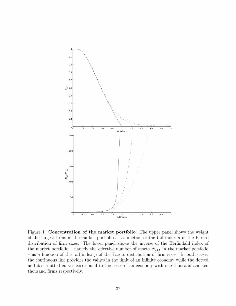
To illustrate this distribution, the upper panel of Figure 1 depicts the value of the

weight of the largest firm in the market portfolio while the lower panel shows the inverse of the

Herfindahl index as a function of µ. The inverse of the Herfindahl index can be understood

as the effective number of assets in the portfolio. It is the exact number of assets required to

construct an equally-weighted portfolio with the same concentration (same Herfindahl index)

as the original portfolio, since the Herfindahl index of any equally-weighted portfolio made

of N assets is just H = 1/N . This allows us to interpret the inverse of the Herfindahl index

as the effective number of assets of a portfolio. The solid curves show the limit situation

of an infinite economy while the dotted and dash-dotted curves account for the finiteness

of the economy. The dotted curve refers to the case where only one thousand companies

are traded while the dash-dotted curve corresponds to an economy with ten thousand firms.

The lower panel shows that the number of effective assets, in a market where about one

thousand to ten thousand assets are traded, ranges between 35 and 60 if the distribution of

market capitalizations follows Zipf’s Law (µ = 1). This observation remains robust to slight

departure from µ = 1. Clearly, there is a substantial difference between an economy with a

large number of assets trades as is the case of the US economy and the case where there is

an infinite number of assets.

To be a little more general, we can consider an economy where the firm sizes are

randomly drawn from a power law distribution of size. Proposition 2 in Appendix A focuses

on this situation in detail and shows no qualitative changes with respect to the result (8)

derived for deterministic firm sizes. Concretely, for an economy in which the distribution

of firm sizes follows Zipf’s law, we obtain a typical value of HN of about 5% for a market

where 8, 000 assets are traded.4 This value is much larger than the concentration index of the

equally-weighted portfolio of all assets which would be of the order of 0.012%. Intuitively,

HN ' 5% means that there are only about 1/Hn ' 20 effective assets in a supposedly well-

diversified portfolio of 8, 000 assets. This order of magnitude is the same as the one obtained

above where the distribution of firm sizes was assumed to follow a deterministic sequence.

4These figures are compatible with the number of stocks currently listed on the Amex, the Nasdaq andthe NYSE.

5

2.2 Correlated residuals in factor models

Consider an economy with N firms with stock returns determined according to the following

factor model

r = α + βm · (rm − E [rm]) + ε, (9)

where

• r is the random N × 1 vector of asset returns;

• α = E [r] is the N × 1 vector of asset return mean values. We do not make any

assumption on the ex-ante mean-variance efficiency of the market portfolio or on the

absence of arbitrage opportunity, so that α is not, a priori, specified;

• rm is the random return on the market portfolio;

• βm is the N × 1 vector of the stocks’ loadings on the market factor;

• ε is the random N × 1 vector of disturbance terms with zero average E [ε] = 0 and

covariance matrix Ω = E [ε · ε′], where the prime denotes the transpose operator. The

disturbance terms are assumed to be uncorrelated with the market return rm and the

factors φi.

We posit a single factor equal to the market portfolio return for simplicity; all our results

hold if there were additional risk factors in the model.

It would be natural to assume that (i) Ω is diagonal in order to interpret the ε as

the specific risk of the assets but, as we shall see below, there is an internal consistency

condition that makes this impossible and forces the disturbances ε to be correlated. A

weaker hypothesis on Ω would be that (ii) all its eigenvalues are uniformly bounded from

above by some constant λ independent of the size of the economy. This implies that the

covariance matrix of the stock returns defined as

Σ = E[(r − α) (r − α)

′]= ββ ′ · Var [rm] + Ω, (10)

has an approximate factor structure, according to the definition in Chamberlain (1983) and

Chamberlain and Rothschild (1983). But these two assumptions (i) and (ii) are in fact

equivalent, as shown by Grinblatt and Titman (1985). Indeed, a simple repackaging of the

6

N security returns into N new returns constructed by forming N portfolios of the primitive

assets allows us to get a new formulation of expression (9) with mutually uncorrelated

disturbance terms.

To understand why the disturbance terms cannot be uncorrelated, let us first denote

by wm the vector of the weights of the market portfolio. Accounting for the fact that the

market factor is itself composed of the assets that it is supposed to explain, the model must

necessarily fulfill the internal consistency relation

rm = w′m · r. (11)

Left-multiplying (9) by w′m, the internal consistency condition (11) implies the following

relation

(w′m · β − 1) · (rm − E [rm]) + w′

m · ε = 0 . (12)

Then, by our assumption of absence of correlation between rm and ε, it follows trivially that

w′m · ε = 0 almost surely, (13)

while

w′m · β = 1. (14)

An important consequence of this result is the breakdown of the standard assumption

of independence (or, at least, of the absence of correlation) between the non-systematic

components of the returns of securities, pointed out by several authors (Fama 1973, Sharpe

1990). This correlation between the disturbance terms may a priori pose problems in

the pricing of portfolio risks: the systematic risk of a portfolio is totally captured by its

exposure to the market portfolio if (and only if) the disturbance terms can be averaged

out by diversification. Previous authors have suggested that this is indeed what happens

in economies in the limit of a large market N → ∞, for which the correlations between

the disturbance terms are expected to vanish asymptotically and the internal consistency

condition seems irrelevant. For example, while Sharpe (1990, footnote 13) concluded that,

as a consequence of equation (13), at least two of the disturbances, say εi and εj, must

be negatively correlated, he suggested that this problem would disappear in economies

with infinitely many securities. Actually, contrary to this belief, we show below that

even for economies with infinitely many securities, when the companies exhibit a fat-

7

tailed distribution of sizes as they do in reality, the constraint (13) leads to the important

consequence that the risk a well-diversified portfolio does not reduce to its market risk even

in the limit of a very large economy. A significant proportion of asset-specific risk remains

which cannot be diversified away by the simple aggregation of a very large number of assets.

The fact that the disturbance terms ε in the market model (9) are correlated according

to the condition (13) means that there exists at least one common factor z in the residuals,

so that ε can be expressed as

ε = γ · z + η , (15)

where γ is the vector of loading of the factor z.5 For simplicity, we choose η to be a vector

of uncorrelated residuals with zero mean.6 Since w′mε = 0, z and η are not independent from

one another and we have

z = −w′mη

w′mγ

, (16)

provided that w′mγ 6= 0. Therefore, in this framework, z is not actually a factor in the usual

sense of the term since it is correlated with η. We refer to it as an “endogenous” factor. The

market model (9) then becomes

r = α + β · (rm − E [rm]) + γ · z + η, (17)

with

• Cov(rm, z) = Cov(rm, η) = 0, from the absence of correlation between rm and ε;

• Var [η] = ∆, where ∆ is a diagonal matrix;

• Var [z] = w′m∆wm

(w′mγ)2

;

• Cov(z, η) = − 1w′

mγ· w′

m∆.

5Our only requirement is that the covariance matrix of ε exhibits an eigenvalue that goes to infinity in thelimit of an infinite economy, when HN does not go to zero. In contrast, when HN goes to zero as N → ∞, thelargest eigenvalue should remain bounded. This requirement derives simply from the results of Chamberlain(1983) and Chamberlain and Rothschild (1983), who have linked the existence of K unbounded eigenvalues(in the limit N → ∞) of the covariance matrix of the asset returns to a unique approximate factor structure,such that the K associated eigenvectors converge and play the role of K factor loadings.

6It would be enough to assume that all the eigenvalues of the covariance matrix of η are positive anduniformly bounded by some positive constant (Grinblatt and Titman 1983).

8

Below we show that factor z matters for asset pricing when the distribution of firm sizes is

fat tailed, even when the number of firms goes to infinity. We therefore name factor z the

Zipf factor.

To show that the correlation between two disturbance terms εi and εj is not negligible

in an infinite size market, we can evaluate their typical magnitude. To simplify the notation,

and without loss of generality, rescale the vector γ by w′mγ, so that the relation (16) becomes

z = −w′mη, (18)

with w′mγ = 1. The covariance matrix Ω of ε is

Ω = (w′m∆wm) γγ′ − γw′

m∆ − ∆wmγ′ + ∆. (19)

Assuming, for instance, that all the γi’s are equal to one (the condition w′mγ = 1 is then

automatically satisfied from the normalization of the weights wm), the correlation between

εi and εj (i 6= j) reads

ρij =HN − wm,i − wm,j√

(1 + HN − 2wm,i) (1 + HN − 2wm,j), (20)

=HN

1 + HN·(1 + O(wm,i(j)/HN )

). (21)

Expression (21) shows that, provided the market portfolio is sufficiently well-diversified so

that the weight of each asset and the concentration index goes to zero in the limit of a

large market (N → ∞), the correlations ρij between any two disturbance terms go to zero

as usually assumed. However, as soon as HN goes to zero more slowly than 1/N , the

largest eigenvalue of the correlation matrix, associated with the (asymptotic) eigenvector

1 = (1, 1, . . . , 1)′, is λmax,N ' N · HN

1+HNand goes to infinity as the size of the economy grows

indefinitely. This clearly shows that the correlations between the disturbance terms will

generally be important when the distribution of firm sizes has fat tails.

The question that we now have to address is whether these correlations challenge the

usual assumption that well-diversified portfolios have only factor risk and no residual risk.

For this, let us consider a well diversified portfolio wp, i.e., a portfolio such that ||wp||2 → 0

as the size of the economy goes to infinity. From equation (19), the residual variance of this

portfolio, namely the part of the variance of the portfolio that is not ascribed to systematic

9

risk factors, reads

w′pΩwp = (w′

m∆wm)(γw′

p

)2 − 2 (w′m∆wp) (γ′wp) + w′

p∆w′p . (22)

In addition to our previous hypothesis that ∆ is a diagonal matrix, we assume that its

entries are uniformly bounded from below by some positive constant c1 and from above by

some constant c2 < ∞ and that |γw′p| is uniformly bounded from below by some positive

constant d1 and from above by some finite constant d2 (this is the case, for instance, when

one considers γ equal to a vector of ones). Then

w′p∆w′

p ≤ c2 · ||wp||2 → 0, (23)

|(w′m∆wp) (γ′wp)| ≤ c2 · d2 · ||wm|| · ||wp|| → 0, (24)

and

c1 · d1 · ||wm||2 ≤ (w′m∆wm)

(γw′

p

)2 ≤ c2 · d2 · ||wm||2, (25)

so that

w′pΩwp ∼ K · HN , K > 0, as N → ∞. (26)

Therefore, the residual variance w′pΩwp of any “well-diversified portfolio” wp goes to zero, as

the size N of the economy goes to infinity, if and only if the concentration index HN of the

market portfolio goes to zero. In the case of a real economy with µ = 1, Proposition 2 of

Appendix A shows that the Herfindahl index HN of the market portfolio goes to zero but at

the particularly slow decay rate of 1/(ln N)2. As a consequence, the residual variance may

still account for a significant part of the total portfolio variance.

2.3 The Zipf factor and asset pricing

In his article establishing the arbitrage pricing theory, Ross (1976, p. 347) explicitly assumes

that the disturbance terms in the factor model (9) are “mutually stochastically uncorrelated,”

which is inconsistent with the constraint (13) if we assume that the factors (or at least some

of them) can be replicated by portfolios. Indeed, the derivation of the APT results from the

construction of a well-diversified arbitrage portfolio (step 1 in Ross (1976, p. 342)) chosen

to have no systematic risk (step 2). The fact that this arbitrage portfolio has no specific

risk in the limit of a large number of assets (law of large numbers) conditions the results of

10

steps 3 and 4. Unfortunately, as shown in the previous section, if one of the factors (e.g., the

market) is replicated by a portfolio whose weights are distributed according to a sufficiently

fat-tailed distribution, the specific risk of this portfolio cannot be diversified away. In that

case, the conclusion from steps 3 and 4 in Ross (1976) breaks down.

Alternatively, some authors have derived pricing results when the residuals exhibit

correlation. In particular, Chamberlain (1983) and Chamberlain and Rothschild (1983) have

developed the appropriate formalism to deal with this problem, while Stambaugh (1982) and

Ingersoll (1984) have provided sharp pricing bounds in the presence of correlation between the

error terms. Basically, when all the eigenvalues of the residual covariance matrix are bounded

as more and more assets are added to the market, the APT still holds. In contrast, when

some eigenvalues grow without bound, the factors associated with these eigenvalues must

be split off from the residuals and considered as new explaining factors that potentially are

priced. This argument is at the basis of the choice of the specification (15) of the dependence

structure of the disturbances of our market model. Therefore, if we explicitly include our

Zipf factor z in the analysis, the original derivation of Ross’ results still holds, as shown by

Chamberlain (1983). Indeed, a key technical assumption for the APT to hold is that the

ε’s (in equation (9)) are “sufficiently independent to ensure that the law of large numbers

holds” (Ross 1976, p. 342) and, as explained in the previous sections, this condition breaks

down. Nonetheless, this condition holds for the residuals η defined by equations (15-17).

Then, for the one factor model (17), we obtain the following result.

Proposition 1 Consider a market where N assets are traded and for which the internal

consistency condition (13) holds, so that the returns of the set of assets obey the following

dynamics: r = E [r]+β ·(rm − E [rm])+γ ·z+η, where z is the (zero-mean) additional factor

resulting from the internal consistency condition and rm is uncorrelated with z and with the

centered disturbance vector η. Then, under the usual assumptions required for the APT to

hold, the expected return on asset i satisfies

E [ri] − rf = βi · (E [rm] − rf ) + (γi − γm · βi) · (E [rz]− rf ) , (27)

where rf denotes the risk free interest rate and E [rz] ≥ rf is the expected return on any

portfolio wz with no market exposure, w′z · β = 0, with unit exposure to the Zipf factor z,

w′z · γ = 1, and which is well-diversified in the sense that the variance of the new residuals

Var [wz · η] goes to zero as the number N of assets goes to infinity. γm = w′m ·γ is the gamma

11

of the market portfolio.

The proof of this result proceeds as follows. Starting from the model (17) and following step

by step the demonstration of theorems I and II in Ross (1976), we get the asymptotic result

E [r] = ρι + λ1β + λ2γ, (28)

where ρ, λ1 and λ2 are three non-negative constants and ι denotes a vector of ones. Their

values are determined by the expected return of the market portfolio wm, of the portfolio wz

and of any other well-diversified portfolio with no systematic risk. This leads to identifying ρ

with rf , λ2 with (E [rz]− rf ) and λ1 with −γm · (E [rz] − rf)− rf . The quantity γm = w′m · γ

never vanishes, due to the dependence of the residuals.

Two comments are in order. First, expression (27) looks like a standard APT

decomposition of the risk premia of the expected return of a given asset i weighted by their

factor loading, except for one important feature: the risk premium due to the Zipf factor has

its amplitude controlled by the factor loading γi (as usual) corrected by the unusual term

−γmβi. In a standard factor decomposition, it is always convenient to impose γm ≡ ~w′m.~γ = 0

so that the contribution to the total risk premium due to any factor is proportional to its

corresponding factor loading γi. In the case of the Zipf factor, this is intrinsically impossible.

In this sense, expression (27) is not the result of a standard factor decomposition. The

pricing equation (27) highlights the contribution of the Zipf factor to the total risk premium

of a given asset. As we shall see below, the fact that the factor loading βi on the market

portfolio contributes to the amplitude of the risk premium due to the Zipf factor provides

an interesting interpretation of the book-to-market effect.

Second, when the market portfolio is well-diversified, the contribution of the Zipf

factor vanishes asymptotically so that the risk premium associated with this risk factor goes

to zero in the limit of an infinitely large market.

The pricing formula given by proposition 1 offers an interesting new insight into the

valuation of asset prices. However, to take it to the data, we still need to identify empirically

the Zipf factor. There are many ways to do this. We could, for instance, identify the Zipf

factor from a factor analysis of the residuals of the market model. However, we follow a

simpler route. Recall that the risk premium associated with the Zipf factor is due to the

exposure of well-diversified portfolios to residual risk. Therefore, well-diversified portfolios

12

such as the equally-weighted portfolio are particularly sensitive to this risk. We therefore

use as a simple proxy for the Zipf factor the difference in returns between the equal-weighted

and the value-weighted market portfolios. The numerical simulations presented in section B

of the Appendix show that this choice does a good job of capturing the systematic risk in the

residuals of the market model and the corresponding risk premium. We also checked (results

not reported) that this proxy for the Zipf factor correlates highly with the first principal

component of the residuals from the market model.

3 Empirics

This section examines the empirical performance of the Zipf model, contrasting it with the

market model and the Fama-French model. Table 1 offers summary statistics for the value-

weighted and equal-weighted market portfolios, the Zipf factor, and the Fama-French size

(SMB) and value (HML) factors (see Fama and French (1993) for details on the construction

of these two portfolios). The Sharpe ratios of the Zipf factor is 0.11 (0.39 annualized),

of the same magnitude as the market or the HML portfolios and higher than the SMB

portfolio. The Zipf factor’s correlation with the market is 0.38, which is of the same order

as the correlations between the factors SMB and HML and the market factor (0.33 and 0.22

respectively). The Zipf portfolio is highly correlated with the SMB portfolio as would be

expected.

We test the Zipf model with the following time-series regression:

ri,t − rf,t = αi + βi · (rm,t − rf,t) + γi · (rz,t − rf,t) + εi(t) . (29)

We also estimate similar time-series regressions for the market and the Fama-French models.

As test assets, we use the monthly excess returns of twenty-five value-weighted portfolios

sorted by the quintiles of the distribution of size and book-to-market and the returns of

thirty value-weighted industry portfolios.7 Tables 2 and 3 present our results for the period

from July 1931 to December 2005.

Each panel of Table 2 shows alphas, corresponding t-statistics, and R2 for the test

7We have used the monthly data available on Professor French’s website for the 25 portfolios sorted bysize and book-to-market, the thirty industry portfolios, the market factor, the risk-free interest rate, and thefactors SMB and HML.

13

portfolios under each asset pricing model. The number below each square array of numbers

is the average of the absolute values above. The mean absolute alpha is 0.22 for the market

model, 0.16 for the Zipf model, and 0.13 for the Fama-French model. The average mispricing

is thus considerably lower in the Zipf and Fama-French models than in the market model.

There is very little difference between the Zipf and Fama-French models. This is remarkable

since the Zipf model only has two factors whereas Fama-French has three and because of

the remark in Lewellen et al. (2006) that the Fama-French factors are almost guaranteed

to perform well for the set of the 25 double sorted portfolios because they have a strong

factor structure (the three Fama-French factors explain more than 90% of the variation of

the time-series of the portfolios’ returns). The cross-section structure of the pricing errors is

similar in both models, with the largest mispricings occurring for small value firms. Indeed,

these are the portfolios where the alphas are statistically significant as can be assessed from

the t-statistics. The average R2 across the test portfolios is 0.77 in the market model, 0.86

in the Zipf model, and 0.91 in the Fama-French model. We find that the Zipf factor adds

substantial explanatory power for the time series of returns of the test portfolios relative to

the market model.

Table 3 presents similar statistics for industry portfolios. Here we see that the

performance of the three models is substantially the same. The mean absolute alphas are

0.15, 0.17, and 0.19 for the market model, the Zipf model, and the Fama-French model,

respectively. And, as can be seen from the t-statistics, the three models fail in almost the

same industries. The explanatory power of the three models is also similar to each other, with

R2 ranging from 0.64 to 0.67, much lower than for the size and book-to-market portfolios.

4 Conclusion

Starting from a model in which the only a priori systematic risk is the market portfolio, we

show that there is a new source of significant systematic risk that should be priced. This new

risk factor arises from a simple internal consistency condition whereby the market portfolio

is made of the very assets whose returns it is supposed to explain. The new factor becomes

important when the distribution of the capitalization of firms is sufficiently fat-tailed as is

the case of real economies as documented abudantly since Zipf (1949). We therefore term

the new factor the Zipf factor. We show that our two-factor Zipf model performs empirically

as well as the three-factor Fama-French model in the cross-section of stocks.

14

Appendix

A Concentration of the market portfolio when the

distribution of firm sizes follows a power law

We consider an economy where firm sizes are randomly drawn from a power law distribution.

By application of the generalized law of large numbers (Feller 1971, Gnedenko and

Kolmogorov 1954, Ibragimov and Linnik 1975) and using standard results on the limit

distribution of self-normalized sums (Darling 1952, Logan et al. 1973), we can state the

following result.8

Proposition 2 The asymptotic behavior of the concentration index HN is the following:

1. provided that E[S2] < ∞,

HN =1

N

E [S2]

E [S]2+ op(1/N);

2. provided that S is regularly varying with tail index µ = 2 and sµ · Pr [S > s] → c as

s → ∞,

HN =c

E [S]2

lnN

N+ op

(1

N lnN

);

3. provided that S is regularly varying with tail index µ ∈ (1, 2) and sµ ·Pr [S > s] → c as

s → ∞,

HN =

[πc

2Γ(

µ2

)sin µπ

4

]2/µ1

E [S]2· 1

N2−2/µ· ξN + op

(1

N2−2/µ

),

where ξN is a positive free parameter characteristic of the distribution of firm sizes

in the market under consideration. In the limit of large markets, the unconditional

8For simplicity, we have assumed that the firm sizes Si are independent. Proposition 2 can however begeneralized to the more realistic case where firm sizes are not independent. Under mild mixing conditions,the results remain the same up to a scale factor (Jakubowski 1993, Davis and Hsing 1995).

15

distribution of this parameter is the stable law S(µ/2, 1);9

4. provided that S is regularly varying with tail index µ = 1 and sµ · Pr [S > s] → c as

s → ∞,

HN =π

2 · ln2 N· ξN + Op

(1

ln3 N

),

where ξN is a positive free parameter characteristic of the distribution of firm sizes

in the market under consideration. In the limit of large markets, the unconditional

distribution of this parameter is the Levy law S(1/2, 1);

5. provided that S is regularly varying with tail index µ ∈ (0, 1) and sµ ·Pr [S > s] → c as

s → ∞,

HN =4

π1/µ

[Γ

(1 + µ

2

)cos

πµ

4

]2/µ

· ξN ,

where ξN is a positive free parameter characteristic of the distribution of firm sizes

in the market under consideration. In the limit of large markets, the unconditional

distribution of this parameter is given by the limit law of the ratio ζN

ζ′2N, where ζN and

ζ ′N denote two sequences of strongly correlated positive random variables that converge

in law to S(µ/2, 1) and S(µ, 1) respectively;10

6. provided that S is slowly varying11,

HN → 1, a.s.

As a consequence of the fourth statement of the proposition above, for economies in

which the distribution of firm sizes follows Zipf’s law (µ = 1) the asymptotic behavior of the

concentration index HN of the market portfolio is given by

HN ' π

2 · (lnN)2 · ξN , (30)

9The stable law S(α, β) has characteristic function ψα,β(s) =

exp

[−|s|α + isβ tan απ

2|s|α−1

]α 6= 1,

exp[−|s| − isβ 2

π· ln s

]α = 1,

with β ∈ [−1, 1].10 More precisely, the sequence of random vectors (ξN , ζN )′ converges to an operator-stable law with stable

marginal laws S(µ/2, 1) and S(µ, 1) respectively, and a spectral measure concentrated on arcs ±(x, x2).The full characterization of the spectral measure is beyond the scope of this article (see (Meerschaert andScheffler 2001, Section 10.1) for details).

11The random variable S is slowly varying if its distribution function F satisfies limx→∞1−F (tx)1−F (x) = 1, for

all t > 0. It corresponds to the limit case where S is regularly varying with µ→ 0.

16

where ξN is a sequence of positive random variables with stable limit law S(1/2, 1), namely

the Levy law with density

f(x) =1√2π

· x−3/2e−12x , x ≥ 0. (31)

This shows that, even if the concentration of the market portfolio goes to zero in the limit

of an infinite economy, it goes to zero extremely slowly as the size N of the economy

diverges. Accounting for the fact that the numeric factor ξN in (30) is a specific realization

(characteristic of the state of the market under consideration) of a random variable with

asymptotic law given by the Levy law (31) whose median value is approximately equal to

2.198, a typical value of HN is 4 − 5% for a market where 7, 000 to 8, 000 assets are traded.

This value is much larger than the concentration index of the equally-weighted portfolio

which would be of the order of 0.012 − 0.014%. Intuitively, HN ' 4 − 5% means that

there are only about 1/Hn ' 20 − 25 effective assets in a typical portfolio supposedly well-

diversified on 7, 000 to 8, 000 assets. This order of magnitude is the same as the one obtained

in the example where the distribution of firm sizes was assumed to follow a deterministic

sequence.

B Analysis of synthetic markets generated numerically

In order to assess the impact of the internal consistency factor in real stock markets of finite

size, we present in table 4 the results of numerical simulations of synthetic markets with

respectively N = 1, 000 and N = 10, 000 traded assets. We construct the synthetic markets

according to the market model (17) where the only explicit risk factor is the market but

taking into account the dependence in the residuals. We take the initial distribution of the

capitalization of firms to be the Pareto distribution

Pr [S ≥ s] =1

sµ· 1s≥1 . (32)

We investigate various synthetic markets characterized by different tail indices µ, from

µ = 1/2 (deep in the heavy-tailed regime), µ = 1 (borderline case often referred to as

the Zipf law when expressed with sizes plotted as a function of ranks), to µ = 2 (for which

the central limit theorem holds and standard results are expected). It is important to stress

17

that the results presented in table 4 are insensitive to the shape of the bulk of the distribution

of firm sizes, and only the tail Pr [S ≥ s] ∼ s−µ, for large s, matters.

The three values of the tail index µ equal to 2, 1 and 1/2 correspond to the three

major behaviors of the residual variance of a “well-diversified” portfolio, namely the part of

the total variance related to the disturbance term ε only

• for µ = 2, the residual variance goes to zero as 1/N , so that the market return should

be the only relevant explaining factor if the number of traded assets is large enough;

• for µ = 1, the residual variance goes very slowly to zero, so that one can expect a

significant contribution to the total risk and a strong impact of the Zipf factor z for

large (but finite) market sizes;

• for µ = 1/2, the residual variance does not go to zero and one can expect that the

contribution of the residual variance to the total risk remains a finite contribution as

the size of the market increases without bounds.

For each value µ = 2, µ = 1 and µ = 1/2, we generate 100 synthetic markets of each

size N = 1, 000 and N = 10, 000. For each market, we construct 20 equally weighted

portfolios (randomly drawn from each market) so that each of the 20 equally-weighted

portfolios is made of 1,000/20=50 assets and 10,000/20=500 assets when N = 1, 000 and

N = 10, 000, respectively. We regress their returns on the returns of the market portfolio

(rm), on the returns of the market portfolio and of the Zipf factor (rm, z), on the returns of the

market portfolio and of the (overall) equal-weighted portfolio (rm, re), on the returns of the

market portfolio and of an arbitrary under-diversified portfolio (rm, ru), and on the returns

of the market portfolio and of an arbitrary well-diversified arbitrage portfolio (rm, ra). Using

the 100 market simulations for each case (µ, N), Table 4 summarizes the mean, minimum

and maximum values of the coefficient of determination R2 of these five regressions of the

20 equally weighted portfolios.

Notice that our model implies according to (16) or (18) that the factor z is correlated

with the residuals. In the regressions, this is not the case. Therefore, it is a priori something

to be concerned about. However, as shown by the results in Table 4, the regression by OLS

works quite well.

For µ = 2, as was expected, the market return is the only relevant factor: it accounts

on average for about 95% and 99% (for N = 1, 000 and N = 10, 000 assets, respectively)

18

of the total variance of the 20 equally-weighted portfolios under considerations. The fact

that the explained variance increases from 95% to 99% when going from N = 1, 000 to

N = 10, 000 assets, results from the standard diversification effect since each portfolio has

more assets. The minimum and maximum values of the R2 remains very close to their

respective mean values.

For µ = 1, the market factor explains a much smaller part of the total variance

compared with the previous case (80% and 88%, respectively for N = 1, 000 and N = 10, 000

assets). As expected, the lack of explanatory power of the market factor is stronger for the

markets with the smallest number N = 1, 000 of traded assets. In addition, the minimum

R2 (1% and 20%, resp.) departs strongly from its mean value. Besides, the regression on

the market factor and the Zipf factor z (which is readily accessible in the case of a numerical

simulation) provides a level of explanation (95% and 99%, respectively) comparable to that of

the case µ = 2 for which full diversification of the residual risk occurs. Moreover, the equally-

weighted portfolio provides the same level of explanation as z itself. This is particularly

interesting insofar as z is not observable in a real market while the return on the equally-

weighted portfolio can always be calculated, or at least proxied. We find more generally

that any well-diversified portfolio provides overall the same explaining power. This result is

simply related to the fact that the Zipf factor z is responsible for the lack of diversification

of “well-diversified” portfolios (when µ is less than but approximatly 1) so that the return

on any “well-diversified” portfolio p reads rp ' αp +βp · rm +E [γ] · z. This suggests that the

equally-weighted portfolio or any well-diversified portfolio, in so far as it is strongly sensitive

to the Zipf factor z, may act as a good proxy for this factor.

In contrast, the regression on any under-diversified portfolio, while improving on the

regression performed just using the market portfolio, remains of lower quality: the gain in

R2 is only 5-6% on average with respect to the regression on the market portfolio alone.

Finally, table 4 shows that the introduction of an arbitrage portfolio does not improve the

regression. This is due to the fact that arbitrage portfolios are not asymptotically sensitive

to the Zipf factor z in the large N limit.

The same conclusions hold qualitatively for synthetic markets generated with µ = 1/2,

with the important quantitative change that the explanatory power of the market factor does

not increase with the market size N . This expresses the predicted property that the Zipf

factor z should have an asymptotically finite contribution to the residual variance as the size

of the market increases without bounds.

19

Finally, our numerical tests confirm that the distributional properties of the γ’s (the

factor loading of the residuals on the Zipf factor z) have no significant impact on the results

of the simulation, provided that E [|γ|] < ∞.

20

References

Alexander, Gordon J., and Jack C. Francis, 1986, Portfolio Analysis (Prentice Hall).

Axtell, Robert L., 2001, Zipf distribution of U.S. firm sizes, Science 293, 1818-1820.

Axtell, Robert L., 2006, Firm sizes: facts, formulae, fables and fantasies, in Claudio

Cioffi-Revilla, ed.: Power Laws in the Social Sciences (Cambridge University Press).

Forthcoming.

Bai, Jushan and Serena Ng, 2002, Determining the Number of Factors in Approximate Factor

Models, Econometrica 70, 191221.

Banz, Rolf W., 1981, The relationship between return and market values of common stocks,

Journal of Financial Economics 9, 3-18.

Basu, S., 1977, Investment performance of common stocks in relation to their price-earning

ratios: A test of the efficient market hypothesis, Journal of Finance 32, 663-682.

Berk, Jonathan B., 1995, A critique of size-related anomalies, Review of Financial Studies

8, 275-286.

Jonathan B. Berk, Richard C. Green and Vasant Naik, 1999, Optimal Investment, Growth

Options, and Security Returns, Journal of Finance 54, 1553-1607.

Bernardo, Antonio E., Bhagwan Chowdry, and Amit Goyal, 2007, Growth Options, Beta,

and the Cost of Capital, Financial Management, forthcoming.

Bingham, Nicholas H., Charles M. Goldie and Jozef L. Teugels, 1987, Regular Variation

(Cambridge University Press).

Blume, Marshall E., 1980, Stock returns and dividend yields: some more evidence, Review

of Economics and Statistics 62, 567-577.

Breiman, L. (1965) On Some Limit Theorems Similar to the Arc-Sin Law, Theory of

Probability and Its Applications 10, 323-329.

Brennan, Michael J., Ashley Wang, and Yihong Xia, 2004, Estimation and test of a simple

model of intertemporal asset pricing. Journal of Finance 59, 1743-1775.

21

Brennan, Michael J., Xiaoquan Liu and Yihong Xia, 2006, Option Pricing Kernels and the

ICAPM, EFA 2006 Zurich Meetings Available at SSRN: http://ssrn.com/abstract=

917911

Campbell, John Y., and Tuomo Vuolteenaho, 2004, Bad beta, good beta, American

Economic Review 94, 1249-1275.

Chamberlain, Gary, 1983, Funds, factors and diversification in arbitrage pricing theory,

Econometrica 51, 1305-1324.

Chamberlain, Gary and Michael Rothschild, 1983, Arbitrage, factor structure, and mean-

variance analysis on large asset markets, Econometrica 51, 1281-1304.

Chan, Louis K.C., Narasimhan Jegadeesh, and Josef Lakonishok, 1996, Momentum

Strategies, Journal of Finance 51, 1681-1713.

Chan, Louis K.C., 1988, On the contrarian investment strategy, Journal of Business 61,

147-163

Chen Nai-Fu, Richard Roll and Stephen A. Ross, 1986, Economic forces and the stock

market, Journal of Business 59, 383-403.

Chopra, Navin, Josef Lakonishok and Jay R. Ritter, 1992, Measuring abnormal performance

: Do stocks overreact? Journal of Financial Economics 31, 235-268

Connor, Gregory, 1982, Asset pricing in factor economies, Doctoral dissertation (Yale

university).

Daniel, Kent D., David A. Hirshleifer and Avanidhar Subrahmanyam, 2001, Covariance risk,

mispricing, and the cross-section of security returns, Journal of Finance 56, 921-965.

Darling, D. A., 1952, The influence of the maximum term in the addition of independent

random variables, Transactions of the American Mathematical Society 73, 95-107.

Davis, Richard A. and Tailen Hsing, 1995, Point process and partial sum convergence for

weakly dependent random variables with infinite variance, The Annals of Probability

23, 879-917.

DeBondt, Werner F. M., and Richard H. Thaller, 1985, Does the stock market overreact,

Journal of Finance 40, 793-805.

22

DeBondt, Werner F. M., and Richard H. Thaller, 1987, Further evidence on investor

overreaction and stock market seasonality, Journal of Finance 42, 557-581.

Dybvig, Philip H., 1983, An explicit bound on individual assets’ deviations from APT pricing

in a finite economy, Journal of Financial Economics 12, 483-496.

Efron, Bradley, and Robert J. Tibshirani, 1993, An Introduction to the Bootstrap (Chapman

& Hall, CRC).

Embrechts, Paul, Claudia Klueppelberg and Thomas Mikosch, 1997, Modelling Extremal

Events for Insurance and Finance (Springer-Verlag, Heidelberg)

Fama, Eugene F., 1973, A Note on the Market Model and the Two-Parameter Model, Journal

of Finance 28, 1181-1185.

Fama, Eugene. ¿F., and Kenneth R. French, 1992, The Cross-Section of Expected Stock

Returns, Journal of Finance 47, 427-465.

Fama, Eugene. F., and Kenneth R. French, 1993, Common Risk Factors in the Returns on

Stocks and Bonds, Journal of Financial Economics 33, 3-56.

Fama, Eugene. F., and Kenneth R. French, 1995, Size and Book-to-Market Factors in

Earnings and Returns, Journal of Finance 50, 131-155.

Fama, Eugene. F., and Kenneth R. French, 1996, Multifactor explanations of asset pricing

anomalies, Journal of Finance 51, 55-84.

Fama, Eugene. F., and Kenneth R. French, 1997, Industry costs of equity, Journal of

Financial Economics 43, 153-193.

Feller, William, 1971, An Introduction to Probability Theory and its Applications (Wiley).

Ferson Wayne E. and Campbell R. Harvey, 1993, The Risk and Predictability of International

Equity Returns, Review of Financial Studies 6, 527-566.

Gabaix, Xavier, 2005, The Granular Origins of Aggregate Fluctuations, Working Paper,

MIT.

Gabaix, Xavier, Parameswaran Gopikrishnan, Vasiliki Plerou, H. Eugene Stanley, 2006,

Institutional Investors and Stock Market Volatility, Quarterly Journal of Economics

121, 461-504.

23

Geluk, J. and L. de Haan (2000) Stable probability distribution and their domains of

attraction: a direct approach, Probability and Mathematical Statistics 21, 169-188.

Gibbons, Michael R., Stephen A. Ross and Jay Shanken, 1989, A test of the efficiency of a

given portfolio, Econometrica 57, 1121-1152.

Gnedenko, Boris V. and Andrey N. Kolmogorov, 1954, Limit Distributions for Sums of

Independent Random Variables (Addison-Wesley).

Grinblatt, Mark, and Sheridan Titman, 1983, Factor pricing in a finite economy, Journal of

Financial Economics 12, 497-507.

Grinblatt, Mark, and Sheridan Titman, 1985, Approximate factor structures: Interpretations

and implications for empirical tests, Journal of Finance 40, 1367-1373.

Harvey, Campbell R., 1991, The world price of covariance risk, Journal of Finance 46, 111-

157.

Huberman, Gur , 1982, A simple approach to arbitrage pricing theory, Journal of Economic

Theory 28, 183-191.

Ibragimov, I. A. and Yu V. Linnik, 1975, Independent and Stationary Sequences of Random

Variables (Wolters-Noordhoff).

Ijri, Yuji, and Herbert A. Simon, 1977, Skew Distribution of Sizes of Business Firms (North-

Holland, Amsterdam).

Ingersoll, Jonathan E., 1984, Some results in the theory of arbitrage pricing, Journal of

Finance 39, 1021-1039.

Jagannathan, Ravi and Yong Wang, 2007, Lazy investors, discretionary consumption, and

the cross-section of stock returns, Journal of Finance Forthcoming.

Jakubowski, Adam, 1993, Minimal conditions in p-stable limit theorems, Stochastic Processes

and their Applications 44, 291-327.

Jegadeesh, Narasimhan, and Sheridan Titman, 1993, Returns to buying winners and selling

losers: Implications for stock market efficiency, Journal of Finance 48, 65-91.

Jegadeesh, Narasimhan, and Sheridan Titman, 2001, Profitability of Momentum Strategies:

An Evaluation of Alternative Explanations, Journal of Finance 56, 699-720.

24

Keim, Donald B., 1985, Dividend yields and stock returns, Journal of Financial Economics

14, 473-489.

King, Benjamin F., 1966, Market and Industry Factors in Stock Price Behavior, Journal of

Business 39, 139-170.

Kullman, Cornelia, 2003, Real estate and its role in asset pricing. Working paper (University

of British Columbia).

Lakonishok, Joseph, Andrei Shleifer, and Robert W. Vishny, 1994, Contrarian investment

extrapolation and risk, Journal of Finance 49, 1541-1578.

Lewellen, Jonathan, Stefan Nagel and Jay Shanken, 2006, A Skeptical Appraisal of Asset-

Pricing Tests, Working paper, Stanford University.

Logan, B. F., C. L. Mallows, S. O. Rice and L. A. Shepp, 1973, Limit distribution of self-

normalized sums, Annals of Probability 1, 788-809.

Lovett, William A., 1988, Banking and Financial Institutions Law in a Nutshell (Second

Edition, West Publishing Co.).

Lintner, John, 1965, The valuation of risk assets and the selection of risky investments in

stock portfolios and capital budgets, Review of Economics and Statistics 47, 13-37.

Mandelbrot, Benoit B., 1997, Fractals and Scaling in Finance (Springer-Verlag).

Marsili, Orietta, 2005, Technology and the Size Distribution of Firms: Evidence from Dutch

Manufacturing, Review of Industrial Organization 27, 303-328.

Meerschaert, Mark M. and Hans-Peter Scheffler, 2001, Limit Distributions for Sums of

Independent Random Vectors: Heavy Tails in Theory and Practice (Wiley).

Mosimann, James E., 1962, On the compound multinomial distribution, the β-distribution

and the correlations among proportions, Biometrika 49, 65-82.

Mossin, Jan, 1966, Equilibrium in a Capital Asset Market, Econometrica 34, 768-783.

Petkova, Ralitsa, 2006, Do the Fama-French factors proxy for innovations in predictive

variables? Journal of Finance 61, 581-612.

25

Polakoff, Murray, and Thomas A. Durkin, 1981, Financial Institutions and Markets, Second

Edition, Houghton Mifflin.

Ramsden, J.J. and Gy. Kiss-Haypa, 2000, Company size distribution in different countries,

Physica A 277, 220-227.

Reinganum, Mark R., 1981, Misspecification of Capital Asset Pricing, Journal of Financial

Economics 9, 19-46.

Richards, Anthony J., 1996, Winner-loser reversals in national stock market indices: Can

they be explained?, Journal of Finance 52, 2129 - 2144

Roll, Richard, 1994, What every CFO should know about scientific progress in financial

economics: What is known and what remains to be resolved, Financial Management

23, 69-75.

Roll, Richard, and Stephen A. Ross, 1984, An Empirical Investigation of the Arbitrage

Pricing Theory, Journal of Finance 35, 1073-1103.

Roll, Richard and Stephen A. Ross, 1984, The arbitrage pricing theory approach to strategic

portfolio planning, Financial Analysts Journal (May/June), 14-26.

Rosenberg, Barr, Kenneth Reid, and Ronald Lanstein, 1985, Persuasive Evidence of Market

Inefficiency, Journal of Portfolio Management 11, 9-16.

Ross, Stephen A., 1976, The Arbitrage Theory of Capital Asset Pricing, Journal of Economic

Theory 13, 341-60.

Rozeff, Michael S., 1984, Dividend Yields Are Equity Risk Premiums, Journal of Portfolio

Management 10, 68-75.

Sharpe, William F., 1964, Capital asset prices: A theory of market equilibrium under

conditions of risk, Journal of Finance 19, 425-442.

Sharpe, William F., 1990, Capital asset prices with and without negative holdings, Nobel

Lecture, December 7, 1990.

Simon, Herbert A., and Charles P. Bonini, 1958, The size distribution of business firms,

American Economic Review 46, 607-617.

26

Stambaugh, Robert F., 1982, Arbitrage pricing with information, Journal of Financial

Economics 12, 357-369.

Stattman, Dennis, 1980, Book Values and Stock Returns, Chicago MBA: Journal of Selected

Papers 4, 25-45.

Treynor, Jack L., 1961, Market Value, Time, and Risk, Unpublished manuscript.

Treynor, Jack L., 1999, Toward a Theory of Market Value of Risky Assets, in Robert A.

Korajczyk, editor.: Asset Pricing and Portfolio Performance: Models, Strategy and

Performance Metrics (Risk Books, London).

Uchaikin, V.V. and V.M. Zolotarev (1999) Chance and Stability (Stable Distributions and

their Applications) Utrecht, VSP International Science Publishers, 570 p.

Wang, Taychang, 1988, Essays in the theory of arbitrage pricing, Doctoral dissertation

(University of Pennsylvania).

Woerheide, Walt and Don Persson, 1993, An Index of Portfolio Diversification, Financial

Review Services 2, 73-85.

Zipf, George K., 1949, Human Behavior and the Principle of Least Effort (Addison-Wesley,

Cambridge, MA), 498-500.

27

Table 1: Summary statisticsMean value, standard deviation and correlation coefficients of the monthly returns on the marketportfolio (excess return over the one month T-bill), on the equally weighted portfolio (excess returnover the one month T-bill), on the ICC factor (spread between the return on the equally weightedportfolio and the market portfolio), on the SMB and the HLM factors over the time period fromJanuary 1927 to December 2005.

CorrelationMean Std Sharpe Re Zipf SMB HML

Rm 0.64% 5.48% 0.12 0.90 0.38 0.33 0.22Re 1.03% 7.52% 0.14 0.74 0.63 0.35Zipf 0.39% 3.48% 0.11 0.86 0.42SMB 0.25% 3.37% 0.07 0.09HML 0.41% 3.60% 0.11

28

Table 2: Empirical results for size and book-to-market portfoliosTests of three asset pricing models – the market model, the Zipf model, and the Fama-French model – with 25 value-weightedportfolios sorted on size and book to market. Data from July 1931 to December 2005 (894 months).

Low 2 3 4 High Low 2 3 4 High Low 2 3 4 HighPanel A: Market model

α t(α) R2

Small -0.52 -0.06 0.25 0.46 0.59 -1.86 -0.24 1.47 2.77 3.01 0.53 0.57 0.67 0.67 0.612 -0.14 0.18 0.34 0.40 0.44 -0.96 1.45 2.99 3.31 2.86 0.72 0.78 0.78 0.76 0.723 -0.10 0.19 0.26 0.33 0.33 -0.89 2.43 3.11 3.36 2.37 0.82 0.86 0.86 0.81 0.764 -0.01 0.06 0.21 0.25 0.19 -0.09 0.91 2.73 2.56 1.33 0.87 0.91 0.87 0.83 0.76

Big -0.04 0.01 0.06 0.01 0.19 -0.69 0.18 0.78 0.07 1.38 0.92 0.91 0.85 0.79 0.68Mean Abs 0.22 1.75 0.77

Panel B: Zipf model (Market + Zipf)α t(α) R2

Small -0.88 -0.44 -0.05 0.14 0.21 -3.85 -2.75 -0.47 1.58 2.04 0.68 0.80 0.87 0.91 0.892 -0.32 -0.04 0.14 0.19 0.17 -2.81 -0.46 1.92 2.42 1.73 0.81 0.91 0.91 0.90 0.883 -0.24 0.09 0.15 0.19 0.14 -2.78 1.36 2.19 2.49 1.23 0.88 0.91 0.90 0.88 0.854 -0.02 0.00 0.14 0.15 0.03 -0.33 0.00 1.97 1.73 0.21 0.87 0.92 0.89 0.86 0.82

Big 0.02 0.05 0.06 -0.04 0.11 0.41 0.94 0.89 -0.36 0.79 0.94 0.92 0.85 0.80 0.71Mean Abs 0.16 1.51 0.86

Panel C: Fama-French model (Market + SMB + HML)α t(α) R2

Small -0.89 -0.45 -0.10 0.05 0.06 -3.77 -3.03 -1.03 0.68 0.69 0.67 0.82 0.89 0.93 0.932 -0.21 -0.05 0.08 0.07 -0.01 -2.49 -0.78 1.32 1.34 -0.19 0.90 0.94 0.94 0.95 0.963 -0.15 0.09 0.08 0.08 -0.07 -2.31 1.48 1.25 1.26 -1.03 0.93 0.92 0.93 0.93 0.944 0.08 -0.03 0.07 0.01 -0.21 1.45 -0.45 1.07 0.12 -2.59 0.93 0.92 0.91 0.92 0.93

Big 0.07 0.04 -0.02 -0.22 -0.09 1.89 0.86 -0.29 -3.47 -0.90 0.95 0.92 0.90 0.93 0.83Mean Abs 0.13 1.43 0.91

29

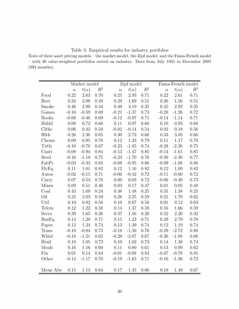
Table 3: Empirical results for industry portfoliosTests of three asset pricing models – the market model, the Zipf model, and the Fama-French model– with 30 value-weighted portfolios sorted on industry. Data from July 1931 to December 2005(894 months).

Market model Zipf model Fama-French modelα t(α) R2 α t(α) R2 α t(α) R2

Food 0.22 2.63 0.70 0.25 2.93 0.71 0.22 2.61 0.71Beer 0.34 2.00 0.49 0.29 1.69 0.51 0.26 1.56 0.51Smoke 0.46 2.99 0.34 0.49 3.19 0.35 0.45 2.92 0.35Games -0.10 -0.59 0.69 -0.21 -1.37 0.73 -0.20 -1.26 0.72Books -0.06 -0.46 0.69 -0.12 -0.97 0.71 -0.14 -1.14 0.71Hshld 0.08 0.72 0.68 0.11 0.97 0.68 0.10 0.93 0.68Clths 0.06 0.42 0.50 -0.02 -0.14 0.54 0.02 0.18 0.56Hlth 0.26 2.36 0.65 0.30 2.73 0.66 0.33 3.05 0.66Chems 0.09 0.95 0.78 0.12 1.33 0.79 0.11 1.17 0.79Txtls -0.10 -0.70 0.67 -0.23 -1.85 0.74 -0.28 -2.26 0.75Cnstr -0.08 -0.94 0.84 -0.13 -1.47 0.85 -0.14 -1.61 0.85Steel -0.16 -1.18 0.75 -0.23 -1.70 0.76 -0.30 -2.30 0.77FabPr -0.03 -0.33 0.85 -0.08 -0.95 0.86 -0.09 -1.08 0.86ElcEq 0.11 1.01 0.82 0.12 1.16 0.82 0.12 1.09 0.82Autos -0.02 -0.15 0.71 -0.06 -0.42 0.72 -0.11 -0.80 0.72Carry 0.07 0.53 0.70 0.00 0.03 0.72 -0.06 -0.49 0.73Mines 0.09 0.51 0.46 0.03 0.17 0.47 0.01 0.05 0.48Coal 0.43 1.69 0.24 0.38 1.48 0.25 0.35 1.38 0.25Oil 0.25 2.03 0.59 0.28 2.25 0.59 0.21 1.70 0.62Util 0.10 0.82 0.58 0.10 0.87 0.58 0.01 0.12 0.63Telcm 0.12 1.22 0.58 0.14 1.47 0.59 0.16 1.66 0.59Servs 0.39 1.65 0.26 0.37 1.56 0.26 0.52 2.26 0.32BusEq 0.14 1.20 0.71 0.15 1.23 0.71 0.29 2.79 0.78Paper 0.12 1.24 0.74 0.13 1.39 0.74 0.12 1.19 0.74Trans -0.10 -0.84 0.73 -0.18 -1.56 0.76 -0.29 -2.72 0.80Whlsl -0.18 -1.21 0.62 -0.29 -2.07 0.67 -0.26 -1.88 0.68Rtail 0.10 1.05 0.73 0.10 1.02 0.73 0.14 1.38 0.74Meals 0.16 1.16 0.60 0.11 0.80 0.61 0.13 0.99 0.62Fin 0.01 0.14 0.84 -0.01 -0.08 0.84 -0.07 -0.78 0.85Other -0.14 -1.17 0.70 -0.19 -1.65 0.71 -0.16 -1.36 0.72

Mean Abs 0.15 1.13 0.64 0.17 1.35 0.66 0.19 1.49 0.67

30

Table 4: Numerical simulationsAverage, minimum and maximum value of the R2 of the regression of the return of 20 equallyweighted portfolios (randomly drawn from a market of N = 1000 and N = 10, 000 assetsaccording to the model (17)) on the market portfolio (rm), on the market portfolio and theinternal consistency factor (rm, f), on the market portfolio and the (overall) equally weightedportfolio (rm, re), on the market portfolio and an under-diversified portfolio (rm, ru) and onthe market portfolio and a well-diversified arbitrage portfolio (rm, ra). Different marketsituations are considered with distributions of firm sizes with tail index µ which varies from0.5 to 2.

N=1000 N=10,000rm rm, f rm, re rm, ru rm, ra rm rm, f rm, re rm, ru rm, ra

Mean 94% 94% 95% 94% 94% 99% 99% 99% 99% 99%µ = 2 Min 90% 93% 93% 90% 90% 99% 99% 99% 99% 99%

Max 96% 96% 96% 96% 96% 100% 100% 100% 100% 100%

Mean 80% 95% 95% 86% 82% 88% 99% 99% 93% 89%µ = 1 Min 1% 91% 91% 42% 17% 20% 99% 99% 66% 20%

Max 95% 100% 100% 95% 95% 99% 100% 100% 99% 99%

Mean 56% 97% 97% 79% 64% 56% 100% 100% 83% 63%µ = 1/2 Min 2% 89% 89% 34% 15% 1% 96% 97% 15% 3%

Max 100% 100% 100% 100% 100% 100% 100% 100% 100% 100%

31

0 0.2 0.4 0.6 0.8 1 1.2 1.4 1.6 1.8 20

0.1

0.2

0.3

0.4

0.5

0.6

0.7

0.8

0.9

1

tail index µ

wm

,1

0 0.2 0.4 0.6 0.8 1 1.2 1.4 1.6 1.8 20

50

100

150

200

250

tail index µ

Nef

f=1/

Hm

Figure 1: Concentration of the market portfolio. The upper panel shows the weightof the largest firms in the market portfolio as a function of the tail index µ of the Paretodistribution of firm sizes. The lower panel shows the inverse of the Herfindahl index ofthe market portfolio – namely the effective number of assets Neff in the market portfolio– as a function of the tail index µ of the Pareto distribution of firm sizes. In both cases,the continuous line provides the values in the limit of an infinite economy while the dottedand dash-dotted curves correspond to the cases of an economy with one thousand and tenthousand firms respectively.

32