Option strategies - Universidade Nova de Lisboa

ARTICLE IN PRESS

Journal of Financial Markets 12 (2009) 391–417

1386-4181/$ -

doi:10.1016/j

�CorrespoE-mail ad

1On leave

www.elsevier.com/locate/finmar

Option strategies: Good deals and margin calls

Pedro Santa-Claraa,1, Alessio Sarettob,�

aUniversidade Nova de Lisboa and NBER, Rua Marques de Fronteira, 20, 1099-038 Lisboa, PortugalbThe Krannert School, Purdue University, West Lafayette, IN 47907-2056, USA

Available online 19 January 2009

Abstract

We provide evidence that trading frictions have an economically important impact on the

execution and the profitability of option strategies that involve writing out-of-the-money put options.

Margin requirements, in particular, limit the notional amount of capital that can be invested in the

strategies and force investors to close down positions and realize losses. The economic effect of

frictions is stronger when the investor seeks to write options more aggressively. Although margins are

effective in reducing counterparty default risk, they also impose a friction that limits investors from

supplying liquidity to the option market.

r 2009 Elsevier B.V. All rights reserved.

JEL classification: G12; G13; G14

Keywords: Limits to arbitrage; Option strategies

Dear Customers,

As you no doubt are aware, the New York stock market dropped precipitously onMonday, October 27, 1997. That drop followed large declines on two previous days.This precipitous decline caused substantial losses in the funds’ positions, particularlythe positions in puts on the Standard & Poor’s 500 Index. [...] The cumulation ofthese adverse developments led to the situation where, at the close of business onMonday, the funds were unable to meet minimum capital requirements for themaintenance of their margin accounts. [...] We have been working with our broker-dealers since Monday evening to try to meet the funds’ obligations in an orderly

see front matter r 2009 Elsevier B.V. All rights reserved.

.finmar.2009.01.002

nding author. Tel.: +1765 496 7591.

dresses: [email protected] (P. Santa-Clara), [email protected] (A. Saretto).

from UCLA. Tel.: +351 21 382 2706.

www.elsevier.com/locate/finmar

dx.doi.org/10.1016/j.finmar.2009.01.002

mailto:[email protected]

mailto:[email protected]

ARTICLE IN PRESS

2Sim

Rosen

return3A l

risk pr

Burasc

(2003)

(2005)

(2006)

P. Santa-Clara, A. Saretto / Journal of Financial Markets 12 (2009) 391–417392

fashion. However, right now the indications are that the entire equity positions in thefunds has been wiped out.Sadly, it would appear that if it had been possible to delay liquidating most of thefunds’ accounts for one more day, a liquidation could have been avoided.Nevertheless, we cannot deal with ‘‘would have been.’’ We took risks. We weresuccessful for a long time. This time we did not succeed, and I regret to say that all ofus have suffered some very large losses.— Letter from Victor Niederhoffer to investors in his hedge funds.

Jackwerth (2000), Coval and Shumway (2001), Bakshi and Kapadia (2003), Bondarenko(2003), Jones (2006), and Driessen and Maenhout (2007) find that strategies that involvewriting put options on the S&P 500 index offer very high Sharpe ratios (‘‘good deals’’)—close to two on an annual basis for writing straddles and strangles.2 In the financeliterature the debate over the relevance of those results in determining whether out-of-the-money (OTM) put options are or are not mis-priced is quite fervid. On one hand, thestrategies’ returns are difficult to justify as remuneration for risk in the context of modelswith a representative investor and standard utility function.3 Even fairly general semi-parametric approaches such as those followed by Bondarenko (2003) and Jones (2006) ornon-standard utility functions, such as in Driessen and Maenhout (2007), have littlesuccess in explaining the high returns. On the other hand, Benzoni et al. (2005) study aneconomy where very low mean reversion in the state variable leads investors to keepbuying options for insurance purposes long after a market crash has occurred, thereforekeeping high prices of put options. Bates (2007) propose to evaluate the historical optionreturns relative to those produced in simulation by commonly used option pricing models.They find no evidence of mis-pricing when using a stochastic volatility model with jumps.A third stream of the literature investigates the impact of demand pressure on option

prices. Bollen and Whaley (2004) show that net buying pressure is positively related tochanges in the implied volatility surface of index options. Garleanu et al. (2005) argue thatthe net demand of private investors affects the way market-makers price options. In theirmodel, high prices are driven by market makers who charge a premium as compensationfor the fact that they cannot completely hedge an unbalanced inventory. In summary,Garleanu et al. argue that demand pressure causes option prices to be higher than theywould otherwise be in the presence of a more widespread group of liquidity providers.Indeed, prices are so high that trading strategies that involve providing liquidity to themarket (such as writing options) appear to earn an exceptionally high returns.On one hand if put options are mis-priced, perhaps because their prices are bid up by

demand pressure, the question of why such trading opportunities have not attracted theattention of sophisticated investors, who do not need to be completely hedged, is still un-answered and therefore deserves attention. On the other hand, if put options are not

ilarly, Day and Lewis (1992), Christensen and Prabhala (1998), Jackwerth and Rubistein (1996), and

berg and Engle (2002) find discrepancies between the empirical and the implicit distribution of the S&P 500

s.

arge set of studies concludes that option prices can be rationalized only by very large volatility and/or jump

emia. See, for example, Bates (1996), Bakshi et al. (1997), Bates (2000), Chernov and Ghysels (2000),

hi and Jackwerth (2001), Benzoni (2002), Pan (2002), Chernov et al. (2003), Eraker et al. (2003), Jones

, Eraker (2004), Liu et al. (2005), Santa-Clara and Yan (2004), Benzoni et al. (2005), Xin and Tauchen

, and Broadie et al. (2006). Bates (2001) introduces heterogeneous preferences while Buraschi and Alexei

consider heterogeneous beliefs.

ARTICLE IN PRESSP. Santa-Clara, A. Saretto / Journal of Financial Markets 12 (2009) 391–417 393

mis-priced and the high put option returns are due to very large premia for volatility and/or jump risk, a question still remains as to the ability of investors participating in themarket. We do not attempt to distinguish between those two alternatives, but simply try tomeasure the impact of margins on the realized return of option trading strategies. In thebroad sense, our paper therefore is focused on developing and testing the hypothesis thatmargin requirements, although effective in reducing counterparty default risk, impose afriction that might significantly blunt the effectiveness of option markets for risk sharingamong investors.

Margin requirements limit the notional amount of capital that can be invested in thestrategies and force investors out of trades at the worst possible times (precisely when theyare losing the most money). Our evidence indicates that, once margins are taken intoaccount, the profitability and the risk-return trade off of the ‘‘good deals’’ is not aseconomically significant as previously documented. Therefore, we argue that these frictionsmake it difficult for investors (non-market-makers) to systematically write options.

Our study analyzes data on S&P 500 options from January of 1985 to April of 2006, aperiod that encompasses a variety of market conditions. We study the effect of twodifferent margining systems: the system applied by the Chicago Board of OptionsExchange (CBOE) to generic customer accounts, and the system applied by the ChicagoMercantile Exchange (CME) to members’ proprietary accounts and large institutionalinvestors. We find that the requirements imposed by the CBOE are more onerous anddifficult to maintain than the requirements imposed by the CME. In both cases, marginsaffect the execution and the profitability of option strategies. In particular, marginsinfluence the strategies along two dimensions: they limit the number of contracts that aninvestor can write, and they force the investor to close down positions. For example, aCBOE customer with an availability of capital equivalent to one S&P 500 futures contractcould write only one ATM near-maturity put contract if she wanted to meet the maximummargin call in the sample. If the investor chose to write more contracts, she would not beable to always meet the minimum requirements. As a consequence, her option positionswould have to be closed. Forced liquidations happen precisely when the strategies arelosing the most money, or in other words when the market is sharply moving against theinvestor’s positions— a sudden decrease of the underlying value or an increase in marketvolatility. Therefore the investor is forced to realize losses. Partial and total liquidationsdue to margin calls also force the investor to execute a larger number of trades, increasingthe importance of transaction costs.

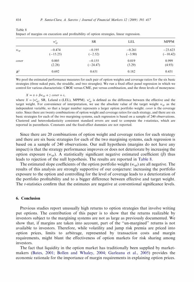
We test for the statistical relationship between the portfolio exposure to options andmeasures that proxy for the execution and the profitability of the strategies. The results ofthis analysis are supportive of our conjecture: increasing the portfolio exposure to theoption and controlling for the level of coverage leads to a deterioration of the portfolioprofitability and to a bigger difference between the effective and the target weight. Weobserve this positive relationship when we consider the Sharpe ratio, the Leland (1999)alpha, and the manipulation-proof performance measure (MPPM) of Ingersoll et al.(2007).

In synthesis, the main result of this paper is that the difference between option‘‘margined’’ realized returns and option ‘‘un-margined’’ returns can be quite substantialwhen investors are subject to margins and do not have unlimited access to capital when themarket is in a downturn state. Consequently, our paper contributes to the literature thatstudies the impact of demand pressure on option prices by showing how frictions limit

ARTICLE IN PRESSP. Santa-Clara, A. Saretto / Journal of Financial Markets 12 (2009) 391–417394

arbitrageurs from supplying liquidity to the market and hence releasing pressure onmarket-makers. In that sense, this study complements the results of Garleanu et al. (2005).Moreover, our results help explain the findings of Jones (2006). Jones considers returnsbefore margins are taken into account and finds that only a portion of the returns can beexplained by jump and volatility factors. We show that part of these ‘‘un-margined’’returns are not available to investors and therefore should not be explainable in terms ofremuneration for risk. Our paper also contributes to the vast literature that studies tradingcosts in option markets (see, for example, Constantinides et al., 2008) by offering evidenceon the effect of a particular source of friction, which has not been explicitly considered:margin requirements.4

Consistent with the arguments of Shleifer and Vishny (1997), Duffie et al. (2002), andLiu and Longstaff (2004) about the limits to arbitrage, our findings could help explain whythe good deals in options prices might be difficult to arbitrage away and why speculativeinvestors do not compete with market-makers to provide liquidity by taking the short sideof the trade in index options. The literature on limits to arbitrage has not reached completeconsensus. While Battalio and Stultz (2006) find no evidence in favor of the limits toarbitrage argument, Ofek et al. (2004), Duarte et al. (2006), and Han (2008) find thatrelative mis-pricings are stronger when there are more impediments to arbitrage activity.Our paper adds to the above studies in providing further empirical evidence in favor of thelimits to arbitrage argument.Under the opposite view that put option prices are perfectly consistent with large risk

premia for volatility and/or jump risk, our results are still interesting in that they documenthow options might not be effective instruments for risk sharing among investors.The rest of the paper is organized as follows. In Section 1 we describe the data. We

explain the option strategies studied in the paper and give summary statistics of thestrategy returns in Section 2. Section 3 describes the margin requirements analyzed in thispaper. In Section 4, we analyze the impact of margin requirements on the execution andthe profitability of the strategies in the case where the investor is allowed to trade inoptions and the risk-free rate. We extend the investment opportunity set to include indexfutures in Section 5. Section 6 concludes.

1. Data

All our main tests are conducted using data provided by the Institute for FinancialMarkets for American options on S&P 500 futures traded at the CME. This datasetincludes daily closing prices for options and futures traded between January 1985 and May2001. We use data from OptionMetrics for European options on the S&P 500 index, whichare traded at the CBOE to estimate bid–ask spreads for various levels of moneyness. Thisdataset includes daily closing bid and ask quotes for the period between January 1996 andApril 2006.

4Few studies consider margin requirements in options: Heath and Jarrow (1987) show that the Black–Scholes

model still holds. Mayhew et al. (1995) and John et al. (2003) study the implication of margins for liquidity and

the speed at which information is incorporated into prices. Driessen and Maenhout (2007) and Driessen et al.

(2008) incorporate margins in portfolio optimization exercises. There is also a vast literature that studies trading

costs in the context of option markets. Some examples are Leland (1985), Figlewski (1989), Bensaid et al. (1992),

Green and Figlewski (1999), Constantinides and Zariphopoulou (2001), Constantinides and Perrakis (2002), and

Constantinides et al. (2008).


To minimize the impact of recording errors and to guarantee homogeneity in the data,we apply a series of filters. First, we eliminate prices that violate basic arbitrage bounds.Second, we eliminate all observations for which the bid is equal to zero, or for which thespread is lower than the minimum ticksize (equal to $0.05 for options trading below $3 and$0.10 in any other cases). Finally, we exclude all observations for which the implied Black(1976) volatility is larger than 200% or lower than 1%.

We construct the option return from the closing of the first trading day of each month tothe closing price of the first trading day of the next month. We obtain a time-series bycomputing the option return in each month of the sample. The returns of the strategies arenot affected by the American nature of the options traded in the CME. We computereturns based on the prices published by the exchange that already include the earlyexercise premium assessed by the market participants. The results we obtain with theEuropean options traded in the CBOE are very similar to the results obtained with theAmerican options traded on the CME.

2. Option strategies

We analyze several option strategies standardized at different moneyness levels. Wefocus on one maturity, corresponding to approximately 45 days, and three different levelsof moneyness, at-the-money (ATM), 5%, and 10% OTM. All the strategies areconstructed so that they involve writing options.

We consider only strategies that involve at least one put contract since those strategieshave been found to generate large returns—see, for example, Coval and Shumway (2001),Bakshi and Kapadia (2003), Bondarenko (2003), Jones (2006), and Driessen andMaenhout (2007). We consider naked and covered positions in put options, delta-hedgedputs, and combinations of calls and puts, such as straddles and strangles.5 A nakedposition is formed simply by writing the option contract. A covered put combines anegative position in the option and a short in the underlying. A delta-hedged put is formedby selling one put contract, as well as delta shares of the underlying. We also studystrategies that involve combinations of calls and puts, such as straddles and strangles. Astraddle involves writing a call and a put option with the same strike and expiration date.A strangle differs from a straddle in that the strike prices are different: write a put with alow strike and a call with a high strike.

2.1. Summary statistics

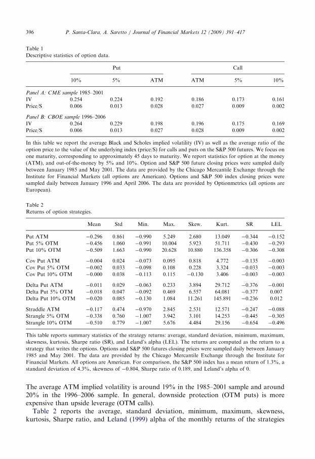
We start by discussing the characteristics of the options used in constructing the monthlyreturns. In Table 1, for any moneyness level, we tabulate the average Black and Scholesimplied volatility and the average price as a percentage of the value of the underlying. Thislast information is essential to understand the magnitude of the portfolio weights that wewill analyze in the following sections and gives us an idea of how expensive the options arerelative to the underlying value. We report results for the S&P 500 futures options (CMEsample) in Panel A and results for the S&P 500 index options (CBOE sample) in Panel B.

5In a previous version of this paper, we used to study a much wider set of option strategies. Although the result

about these strategies are still interesting, we do not report them for the sake of brevity. These results are available

from the authors upon request.

ARTICLE IN PRESS

Table 1

Descriptive statistics of option data.

Put Call

10% 5% ATM ATM 5% 10%

Panel A: CME sample 1985–2001

IV 0.254 0.224 0.192 0.186 0.173 0.161

Price/S 0.006 0.013 0.028 0.027 0.009 0.002

Panel B: CBOE sample 1996–2006

IV 0.264 0.229 0.198 0.196 0.175 0.169

Price/S 0.006 0.013 0.027 0.028 0.009 0.002

In this table we report the average Black and Scholes implied volatility (IV) as well as the average ratio of the

option price to the value of the underlying index (price/S) for calls and puts on the S&P 500 futures. We focus on

one maturity, corresponding to approximately 45 days to maturity. We report statistics for option at the money

(ATM), and out-of-the-money by 5% and 10%. Option and S&P 500 future closing prices were sampled daily

between January 1985 and May 2001. The data are provided by the Chicago Mercantile Exchange through the

Institute for Financial Markets (all options are American). Options and S&P 500 index closing prices were

sampled daily between January 1996 and April 2006. The data are provided by Optionmetrics (all options are

European).

Table 2

Returns of option strategies.

Mean Std Min. Max. Skew. Kurt. SR LEL

Put ATM �0.296 0.861 �0.990 5.249 2.680 13.049 �0.344 �0.152

Put 5% OTM �0.456 1.060 �0.991 10.004 5.923 51.711 �0.430 �0.293

Put 10% OTM �0.509 1.663 �0.990 20.628 10.880 136.358 �0.306 �0.308

Cov Put ATM �0.004 0.024 �0.073 0.095 0.818 4.772 �0.135 �0.003

Cov Put 5% OTM �0.002 0.033 �0.098 0.108 0.228 3.324 �0.033 �0.003

Cov Put 10% OTM �0.000 0.038 �0.113 0.115 �0.130 3.406 �0.003 �0.003

Delta Put ATM �0.011 0.029 �0.063 0.233 3.894 29.712 �0.376 �0.001

Delta Put 5% OTM �0.018 0.047 �0.092 0.469 6.557 64.081 �0.377 0.007

Delta Put 10% OTM �0.020 0.085 �0.130 1.084 11.261 145.891 �0.236 0.012

Straddle ATM �0.117 0.474 �0.970 2.845 2.531 12.571 �0.247 �0.088

Strangle 5% OTM �0.338 0.760 �1.007 3.942 3.101 14.253 �0.445 �0.305

Strangle 10% OTM �0.510 0.779 �1.007 5.676 4.484 29.156 �0.654 �0.496

This table reports summary statistics of the strategy returns: average, standard deviation, minimum, maximum,

skewness, kurtosis, Sharpe ratio (SR), and Leland’s alpha (LEL). The returns are computed as the return to a

strategy that writes the options. Options and S&P 500 futures closing prices were sampled daily between January

1985 and May 2001. The data are provided by the Chicago Mercantile Exchange through the Institute for

Financial Markets. All options are American. For comparison, the S&P 500 index has a mean return of 1.3%, a

standard deviation of 4.3%, skewness of �0.804, Sharpe ratio of 0.189, and Leland’s alpha of 0.


The average ATM implied volatility is around 19% in the 1985–2001 sample and around20% in the 1996–2006 sample. In general, downside protection (OTM puts) is moreexpensive than upside leverage (OTM calls).Table 2 reports the average, standard deviation, minimum, maximum, skewness,

kurtosis, Sharpe ratio, and Leland (1999) alpha of the monthly returns of the strategies


discussed in the previous section.6 As a first attempt, to understand the statisticalproperties of the strategies, we compute the return of a long position in the option, which isfinanced by borrowing at the risk-free rate.

Table 2 is divided into four panels that group strategies with similar characteristics. Theaverage returns of all the strategies are negative across all moneyness levels. Selling 10%OTM put contracts earns 51% per month on average, with a Sharpe ratio of 0.306, and aLeland alpha of 30% (first panel of Table 2). The reward is accompanied by considerablerisk: the strategy has a negative skewness of –10.880, caused by a maximum possible loss of20 times the notional capital of the strategy. These numbers are comparable to thosereported by Bondarenko (2003). Protective put strategies also have negative returns;however, the Sharpe ratios are very small. Similarly to Bakshi and Kapadia (2003), we findthat the delta-hedged returns are all associated with large Sharpe ratios (e.g., the 10%OTM delta-hedged put has an average return of �2:0% per month with a Sharpe ration of�0:236). The Leland alpha, however, is positive at 1.2%, indicating that, according to thatperformance measure, writing delta-hedge puts would not be a good investment. Straddlesand strangles offer high average returns, Sharpe ratios, and Leland alphas, which areincreasing with the level of moneyness: a short position in the ATM straddle returns onaverage 11% per month, with a Sharpe ratio of 0.247 and a Leland alpha of 8.8%, while ashort position in the 10% OTM strangle earns an average 51% per month, with a Sharperatio of 0.654 and a Leland alpha of 49%. These numbers are comparable to thosereported by Coval and Shumway (2001).

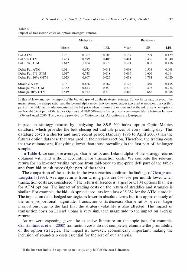
Similar statistics for the European S&P 500 index options, over the period 1996–2006,can be found in the first three columns of Table 4. In that sample, the average strategyreturns are very close to the average returns in the 1985–2001 sample. However, thestrategy volatilities are lower in the 1996–2006 sample, thus leading to higher Sharperatios.

Although the general performance of the strategies is consistent in various sub-samples,the inclusion of the October 1987 crash does change the magnitude of the profitability ofsome strategies. For this reason, we prefer to leave the pre-crash observations in the sampledespite the evidence that a structural break did occur in those years (for example,Jackwerth and Rubistein, 1996; Benzoni et al., 2005), and the fact that the maturitystructure of the available contracts changed after the crash (for example, Bondarenko,2003). Complete summary statistics for the various sub-samples are not reported in thepaper. A brief discussion follows. Let us consider, for example, the 5% OTM put. Theaverage return for the years around the 1987 market crash, January 1985 to December1988, is �25:2%, while in the rest of the sample, January 1989 to May 2001, the strategyaverages �52:1%. Even if we consider the more recent period that starts with the burst ofthe ‘‘Internet bubble,’’ 2001 up to 2006, the return of the S&P 500 index put still averaged�30% per month in a substantially bearish market.

6Leland (1999) provides a simple correction of the CAPM, which allows the computation of a robust risk

measure for assets with arbitrary return distributions. This measure is based on the model proposed by Rubinstein

(1976) in which a CRRA investor holds the market in equilibrium. The discount factor for this economy is the

marginal utility of the investor and expected returns have a linear representation in the beta derived by Leland.

Subtracting Leland’s beta times the market excess return from the strategy returns gives an estimate of the strategy

alpha. Results for the alpha derived from CAPM and the Fama and French (1993) three factor model are very

similar and are available from the authors upon request.


2.2. Statistical significance

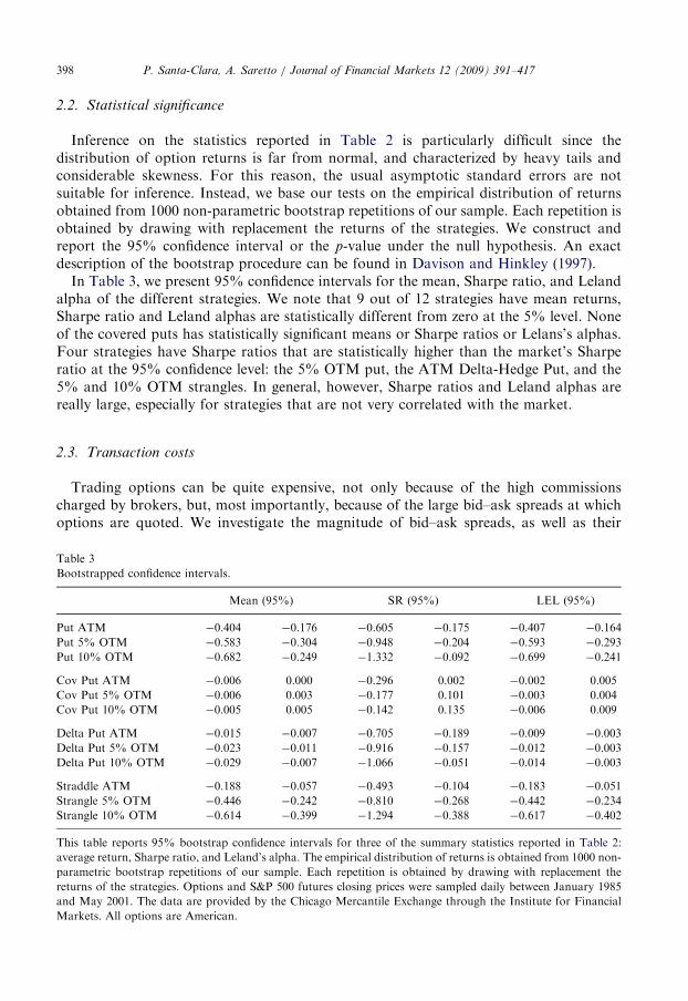
Inference on the statistics reported in Table 2 is particularly difficult since thedistribution of option returns is far from normal, and characterized by heavy tails andconsiderable skewness. For this reason, the usual asymptotic standard errors are notsuitable for inference. Instead, we base our tests on the empirical distribution of returnsobtained from 1000 non-parametric bootstrap repetitions of our sample. Each repetition isobtained by drawing with replacement the returns of the strategies. We construct andreport the 95% confidence interval or the p-value under the null hypothesis. An exactdescription of the bootstrap procedure can be found in Davison and Hinkley (1997).In Table 3, we present 95% confidence intervals for the mean, Sharpe ratio, and Leland

alpha of the different strategies. We note that 9 out of 12 strategies have mean returns,Sharpe ratio and Leland alphas are statistically different from zero at the 5% level. Noneof the covered puts has statistically significant means or Sharpe ratios or Lelans’s alphas.Four strategies have Sharpe ratios that are statistically higher than the market’s Sharperatio at the 95% confidence level: the 5% OTM put, the ATM Delta-Hedge Put, and the5% and 10% OTM strangles. In general, however, Sharpe ratios and Leland alphas arereally large, especially for strategies that are not very correlated with the market.

2.3. Transaction costs

Trading options can be quite expensive, not only because of the high commissionscharged by brokers, but, most importantly, because of the large bid–ask spreads at whichoptions are quoted. We investigate the magnitude of bid–ask spreads, as well as their

Table 3

Bootstrapped confidence intervals.

Mean (95%) SR (95%) LEL (95%)

Put ATM �0.404 �0.176 �0.605 �0.175 �0.407 �0.164

Put 5% OTM �0.583 �0.304 �0.948 �0.204 �0.593 �0.293

Put 10% OTM �0.682 �0.249 �1.332 �0.092 �0.699 �0.241

Cov Put ATM �0.006 0.000 �0.296 0.002 �0.002 0.005

Cov Put 5% OTM �0.006 0.003 �0.177 0.101 �0.003 0.004

Cov Put 10% OTM �0.005 0.005 �0.142 0.135 �0.006 0.009

Delta Put ATM �0.015 �0.007 �0.705 �0.189 �0.009 �0.003

Delta Put 5% OTM �0.023 �0.011 �0.916 �0.157 �0.012 �0.003

Delta Put 10% OTM �0.029 �0.007 �1.066 �0.051 �0.014 �0.003

Straddle ATM �0.188 �0.057 �0.493 �0.104 �0.183 �0.051

Strangle 5% OTM �0.446 �0.242 �0.810 �0.268 �0.442 �0.234

Strangle 10% OTM �0.614 �0.399 �1.294 �0.388 �0.617 �0.402

This table reports 95% bootstrap confidence intervals for three of the summary statistics reported in Table 2:

average return, Sharpe ratio, and Leland’s alpha. The empirical distribution of returns is obtained from 1000 non-

parametric bootstrap repetitions of our sample. Each repetition is obtained by drawing with replacement the

returns of the strategies. Options and S&P 500 futures closing prices were sampled daily between January 1985

and May 2001. The data are provided by the Chicago Mercantile Exchange through the Institute for Financial

Markets. All options are American.

ARTICLE IN PRESS

Table 4

Impact of transaction costs on option strategies’ returns.

Mid-price Bid-to-ask

Mean SR LEL Mean SR LEL

Put ATM 0.251 0.307 0.186 0.197 0.229 0.129

Put 5% OTM 0.463 0.599 0.406 0.401 0.486 0.340

Put 10% OTM 0.612 1.054 0.572 0.521 0.801 0.476

Delta Put ATM 0.011 0.673 0.011 0.008 0.508 0.008

Delta Put 5% OTM 0.017 0.748 0.018 0.014 0.600 0.014

Delta Put 10% OTM 0.023 0.907 0.025 0.018 0.714 0.020

Straddle ATM 0.181 0.666 0.187 0.128 0.460 0.135

Strangle 5% OTM 0.352 0.673 0.350 0.276 0.497 0.274

Strangle 10% OTM 0.519 0.972 0.510 0.400 0.666 0.388

In this table we analyze the impact of the bid-ask spread on the strategies’ returns. For each strategy, we report the

mean return, the Sharpe ratio, and the Leland alpha under two scenarios: trades executed at mid-point prices (left

part of the table) and trades executed at the bid price when options are written and at the ask price when options

are bought (right part of the table). Options and S&P 500 index closing prices were sampled daily between January

1996 and April 2006. The data are provided by Optionmetrics. All options are European.

P. Santa-Clara, A. Saretto / Journal of Financial Markets 12 (2009) 391–417 399

impact on strategy returns by analyzing the S&P 500 index option OptionMetricsdatabase, which provides the best closing bid and ask prices of every trading day. Thisdatabase covers a shorter and more recent period (January 1996 to April 2006) than thefutures option database that was used in the previous section. Therefore, the trading coststhat we estimate are, if anything, lower than those prevailing in the first part of the longersample.

In Table 4, we compare average, Sharpe ratio, and Leland alpha of the strategy returnsobtained with and without accounting for transaction costs. We compute the relevantreturn for an investor writing options from mid-price to mid-price (left part of the table)and from bid to ask price (right part of the table).

The comparison of the statistics in the two scenarios confirms the findings of George andLongstaff (1993). Average returns from writing puts are 5%–9% per month lower whentransaction costs are considered.7 The return difference is larger for OTM options than it isfor ATM options. The impact of trading costs on the return of straddles and strangles issimilar. For example, the bid-ask spread accounts for a loss of 5.3% for the ATM straddle.The impact on delta-hedged strategies is lower in absolute terms but it is approximately ofthe same proportional magnitude. Transaction costs decrease Sharpe ratios by even largerproportions, due to the fact that the strategy volatility is also affected. The impact oftransaction costs on Leland alphas is very similar in magnitude to the impact on averagereturns.

As we were expecting given the extensive literature on the topic (see, for example,Constantinides et al., 2008) transaction costs do not completely eliminate the profitabilityof the option strategies. The impact is, however, economically important, making theinclusion of round-trip costs essential for the rest of our analysis.

7If the investor holds the options to maturity, only half of the cost is incurred.


The evidence presented in this section, which essentially confirms the findings alreadyreported in the vast existing literature, establishes that several strategies involving writingoptions have produced large average returns (even after transaction costs). Many attemptsto directly or indirectly explain this empirical regularity have been proposed: remunerationfor volatility and jump risk, demand pressure, non-standard preferences, and marketsegmentation (see Bates, 2003 for a review). All these factors have an impact on howoptions are priced and might, therefore, be responsible for the ‘‘high’’ put prices thatgenerate the profitability of the option strategies. It is not clear however what portion ofthese profits is attributable to remuneration for risk (see, for example, Jones, 2006).We conjecture that returns to option trading strategies are affected by market frictions,

creating a wedge between the returns that are observable and those that are realizable. Inthe following sections, we investigate the feasibility of these option strategies, focusing inparticular on how margin requirements impact the returns of the strategies.

3. Margin requirements

All the strategies studied in this paper involve a short position in one or more putcontracts. When an investor writes an option, the broker requests a deposit in a marginaccount of cash or cash-equivalent instruments such as T-bills. The amount requestedcorresponds to the initial margin requirement. The initial margin is the minimumrequirement for the time during which that position remains open. Every day amaintenance margin is also calculated. A margin call originates only if the maintenancemargin is higher than the initial margin. If the investor is unable to provide the funds tocover the margin call, the option position is closed and the account is liquidated.Minimum margin requirements are determined by the option exchanges under

supervision of the Security Exchange Commission (SEC) and the Commodity FuturesTrading Commission (CFTC). Margin keeping is maintained by members of clearinghouses.8

There are essentially three types of account that are maintained by members of aclearing house: market-maker accounts, proprietary accounts, and customer accounts. Thedifference among these accounts is that market-maker accounts are margined on their netpositions (short positions can be offset by long positions) while other accounts aremargined on all the existing short positions. In this paper, we study the customer minimummargin requirements imposed by the CBOE, and the proprietary (speculative) accountmargins imposed by the CME to its members. The margin requirements that are applied bythe two clearing houses to members are very similar in their spirit. The CME has a systemcalled Standard Portfolio Analysis of Risk (SPAN), while the OCC has a system calledTheoretical Intermarket Margin System (TIMS). Both systems are based on scenarioanalysis, and in what follows we assume them to be interchangeable.9 Moreover, some

8In the United States there are 11 Derivatives Clearing Organizations registered with the CFTC. Of these, the

CME clears trades on futures and futures options traded at the CME, while the Options Clearing Corporation

(OCC) clears trades on the stock and index options traded at the American Stock Exchange, the Boston Options

Exchange, the CBOE, the International Securities Exchange, the Pacific Stock Exchange, and the Philadelphia

Stock Exchange.9The OCC does not have any available technical documentation that could be used to reconstruct the exact

functioning of the TIMS system. However, conversation with OCC personnel confirmed that the system is similar

to SPAN.


large institutional players, which are not members of a clearing house, have specialarrangements (often through off-shore accounts) to essentially get the same terms asclearing house members. Therefore, the analysis of the margins on customer accounts(retail investors) and on brokers’ proprietary accounts should be sufficient to uncover theimpact of the margining system on the key players in the option market.

3.1. The CBOE minimum margins for customer accounts

The margin requirements for customers depend on the type of option strategy and onwhether the short positions are covered by a matching position in the underlying asset. Themargin for a naked position is determined on the basis of the option sale proceeds, plus apercentage of the value of the underlying asset, less the dollar amount by which thecontract is OTM, if any.10 Specifically, for a naked position in a call or put option, themargin requirement at time t can be found by applying the following simple rules:

�

1

CB

ma

and

clo

Call: Mt ¼ maxðCt þ aSt � ðK � StjK4StÞ;Ct þ bStÞ and
� Put: Mt ¼ maxðPt þ aSt � ðSt � KjSt4KÞ;Pt þ bKÞ
where Ct and Pt are the option settlement prices, a and b are parameters between 0 and 1,St is the underlying price at the end of the day, and K is the strike price of the option.Delta-hedged positions are subject to a composite margin rule: one minus delta of thenaked-put margin plus the margin on the underlying. Combinations are instead marginedby an amount corresponding to the requirement on the call or the put, whichever isgreater, plus the proceeds of the other side.

The quantification of the parameters a and b depends on the type of underlying assetand on the investor trading in the options. For the S&P 500, the CBOE Margin Manualspecifies a ¼ 15% and b ¼ 10%. Nonetheless, brokers may charge clients with highermargins. For example, E-Trade imposes margin requirements to individual investorsaccording to the same formula but with a and b equal to 40% and 35%, respectively.

3.2. The CME minimum margins for member proprietary accounts and large institutional

investors

The SPAN system is a scenario-based algorithm that computes the margins on the basisof the overall risk of a specific account. The purpose of SPAN is to find what the highestpossible loss of a portfolio would be under a variety of scenarios. These scenarios areconstructed by considering changes in the price of the underlying and in the level ofvolatility. At the end of the day, the assets in the account are re-evaluated using an optionpricing model (the default model is Black, 1976) under a range of underlying price andvolatility movements. The scenario losses and profits of the open positions of a particular

0A complete description of how to determine margin requirements for various strategies can be found in the

OE Margin Manual, which can be downloaded from the website: www.cboe.com/LearnCenter/pdf/

rgin2-00.pdf. Note also that, in July 2005, the SEC approved a set of new rules regarding portfolio margining

cross-margining for index options positions of certain customers, thus making the new margining system

ser to the one adopted by the CME, which will be discussed in the next section.

http://www.cboe.com/LearnCenter/pdf/margin2-00.pdf

http://www.cboe.com/LearnCenter/pdf/margin2-00.pdf


account are then examined together and the highest possible loss is chosen to be theminimum margin requirement for that account.11

For example, the current price range for the S&P 500 futures is �$80, while the volatilityrange is �%5.12 SPAN generates 14 scenarios by considering combinations of seven pricechanges (�$80, �2

3� $80, �1

3� $80, 0) and the two volatility changes. In order to account

for the impact of extreme price movements on deep OTM short positions, SPAN alsocomputes potential losses in two additional scenarios, which correspond to a price changeof �3� $80. In these last two scenarios, only one-third of the potential loss is taken intoaccount to determine margins.

3.3. Comparison of the two margining systems

To offer a simple comparison between the two margining systems, we simulate thebehavior of the margin account for a short position in one put option contract. Wecompute the margin for an ATM option with a maturity of 45 days. The underlying price is$100 and the volatility level is 20%. The option price is computed using the Black (1976)formula, using an interest rate equal to 5%. The initial margin requirement is $17.80 and$9.12 for the CBOE and the CME margin system, respectively. We perform a scenarioanalysis of the margin account by simulating movements in the underlying and volatilitylevels. We allow the underlying value to range between $80 and $100 and the volatility levelbetween 20% and 50% and plot the value of the maintenance margin in Panel A of Fig. 1and the corresponding margin calls in Panel B. Margin calls are computed by subtractingthe initial margin from the maintenance requirement. As the underlying price decreasesand the potential loss incurred by the short position in the put becomes larger themaintenance margin also grows. The value of the CBOE maintenance margin is alwayshigher than the corresponding value for the CME. However, since the CME initial marginis lower than the CBOE initial margin, the CME margin calls are higher than thecorresponding CBOE margin calls.

3.4. Margin haircuts

As a first measure of the amount of margins that an investor would have been asked tomaintain in the sample, we calculate the ‘‘haircut’’ ratio, which represents the amount bywhich the required margin exceeds the price at which the option was written. The haircutcorresponds to the investor’s equity in the option position. We compute the ratio asðMt � V0Þ=V 0, where Mt is the margin at the end of each day t, and V 0 is equal to theproceeds received at the beginning of the month: P0 for naked and delta-hedged puts,13

and C0 þ P0 for straddles and strangles.

11A more detailed description of how SPAN works can be found on the CME webpage at the following URL:

http://www.cme.com/clearing/rmspan/span/compont2480.html.12The range of possible movements in the underlying security is selected by the Board of Directors and the

Performance Bond Sub-Committee in order to match the 99th percentile of the historical distribution of daily

price changes. The time series of the SCAN range parameters were obtained directly from the CME.13Note that the proceeds from writing a delta-hedged put is equal to the put price minus the delta of the

underlying value. We decided to compute the haircut as a percentage of only the put price to make the haircut

ratio of a delta-hedged put comparable to the corresponding ratio of a naked put.

http://www.cme.com/clearing/rmspan/span/compont2480.html

ARTICLE IN PRESS

0.2250.275

0.3250.3750.425

0.4758084

8994

99

18

20

22

24

26

28

30

32

underlyingvolatility

CB

OE

mar

gin

0.2250.275

0.3250.375

0.4250.475

8084

8994

99

10

15

20

25

underlying

volatility

CM

E m

argi

n

0.2250.275

0.3250.375

0.4250.475 80

8489

9499

0

2

4

6

8

10

12

14


CB

OE

mar

gin

call

0.2250.275

0.3250.375

0.4250.475

8084

8994

99

0

5

10

15


CM

E m

argi

n ca

ll

Fig. 1. Simulated margin requirements. We consider an ATM put option with a maturity of 45 days. The

underlying price is $100 and the volatility level is 20%. The option price is computed using the Black (1976)

formula, using an interest rate equal to 5%. In Panel A, we plot the value of the maintenance margin when the

underlying price and volatility move. In Panel B, we plot the corresponding margin calls, which are computed by

subtracting the initial margin from the maintenance requirement. We allow the underlying price to range between

$80 and $110 and the volatility between 10% and 50%. The margin call is computed by subtracting the value of

the initial margin requirement, which is equal to $17.80 and $9.12 for the CBOE and the CME margin system,

respectively, from the maintenance margin: (a) Panel A: maintenance margin and (b) Panel B: margin call.

P. Santa-Clara, A. Saretto / Journal of Financial Markets 12 (2009) 391–417 403

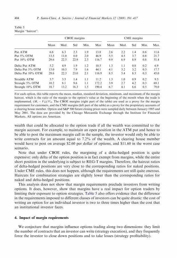
In what follows, we use the CBOE margins as a proxy for the margin requirement forcustomers, and the CME margins as a proxy for the proprietary account marginrequirements for clearing house members and large institutional investors. In Table 5, wereport the mean, median, standard deviation, minimum, and maximum of the haircut ratiofor customers (left part of the table) and proprietary accounts (right part of the table).

On average, a customer must deposit $6.60 as margin (in addition to the option saleproceeds) for every dollar received from writing ATM puts. In our sample, the maximumhistorical haircut ratio for those options, equals 13.8. To put this into perspective, we caninterpret the inverse of the haircut ratio as the maximum percentage of the investor’s

ARTICLE IN PRESS

Table 5

Margin ‘‘haircut’’.

CBOE margins CME margins

Mean Med. Std Min. Max Mean Med. Std Min. Max.

Put ATM 6.6 6.3 2.3 1.9 13.8 2.6 2.2 1.4 0.6 11.6

Put 5% OTM 13.5 11.0 8.0 2.0 46.9 5.5 4.5 3.7 0.8 21.7

Put 10% OTM 29.6 22.5 22.9 2.3 116.7 9.9 6.9 8.9 0.8 51.4

Delta Put ATM 5.2 4.9 1.9 1.2 10.5 1.3 1.1 0.8 0.2 6.9

Delta Put 5% OTM 13.0 10.5 7.9 1.6 44.1 4.1 3.2 3.2 0.3 17.7

Delta Put 10% OTM 29.6 22.3 23.0 2.1 116.9 8.5 5.4 8.3 0.3 45.0

Straddle ATM 3.7 3.5 1.4 1.1 11.2 1.3 1.0 0.9 0.2 9.5

Strangle 5% OTM 10.2 8.1 9.6 1.1 172.2 3.9 2.7 4.2 0.3 69.1

Strangle 10% OTM 18.7 13.2 16.3 1.5 190.4 6.7 4.1 6.6 0.5 79.0

For each option, this table reports the mean, median, standard deviation, minimum, and maximum of the margin

haircut, which is the ratio of the margin to the option’s value at the beginning of the month when the trade is

implemented, ðMt � V0Þ=V0. The CBOE margins (right part of the table) are used as a proxy for the margin

requirement for customers, and the CMEmargins (left part of the table) as a proxy for the proprietary accounts of

a clearing house member. Option and S&P 500 future closing prices were sampled daily between January 1985 and

May 2001. The data are provided by the Chicago Mercantile Exchange through the Institute for Financial

Markets. All options are American.


wealth that could be allocated to the option trade if all the wealth was committed to themargin account. For example, to maintain an open position in the ATM put and hence tobe able to post the maximum margin call in the sample, the investor would only be able towrite contracts for an amount equal to 7.2% of the wealth. A clearing house memberwould have to post on average $2.60 per dollar of options, and $11.60 in the worst casescenario.Note that under CBOE rules, the margining of a delta-hedged position is quite

expensive: only delta of the option position is in fact exempt from margins, while the entireshort position in the underlying is subject to REG-T margins. Therefore, the haircut ratiosof delta-hedged positions are very close to the corresponding ratios for naked positions.Under CME rules, this does not happen, although the requirements are still quite onerous.Haircuts for combination strategies are slightly lower than the corresponding ratios fornaked and delta-hedged positions.This analysis does not show that margin requirements preclude investors from writing

options. It does, however, show that margins have a real impact for option traders bylimiting their exposure to option strategies. Table 5 also offers evidence that the differencein the requirements imposed to different classes of investors can be quite drastic: the cost ofwriting an option for an individual investor is two to three times higher than the cost thatan institutional investor faces.

4. Impact of margin requirements

We conjecture that margins influence options trading along two dimensions: they limitthe number of contracts that an investor can write (strategy execution), and they frequentlyforce the investor to close down positions and to take losses (strategy profitability).


We test this conjecture in the rest of the paper by analyzing a realistic zero-cost strategy.We assume that at the beginning of every month the investor borrows $1 and allocates thatamount to a risk-free rate account that she uses to cover margins.14 Option contracts arewritten for an amount equivalent to a fraction of the one dollar. We refer to this quantityas the ‘‘target’’ portfolio weight. The initial margin requirement is determined on the baseof the number of contracts corresponding to the target weight.

In implementing the strategy, we assume that, during the month, access to the creditmarket is limited so that the investor’s availability to capital cannot exceed what initiallyborrowed. This is a key assumption without that margins never have a real effect ontrading strategy. However, it is not unrealistic to presume that access to capital becomesmore difficult in instances which would trigger margin calls: high volatility and or largenegative market returns. For example, Brunnermeier and Pedersen (2008) study flight toliquidity/quality in an economy characterized by trading frictions similar to those studiedin this paper. They conclude that margins exacerbate funding liquidity in adverse marketconditions. Therefore, in our setting, margin calls are met by liquidating the investment inthe risk-free rate account. When the balance of the risk-free rate account is not sufficient tomeet the margin call, the option position is liquidated at the option’s closing price. At thatpoint, we allow the investor to open a new position so that the new margin due does notexceed 90% of the available wealth. The 90% level is chosen to prevent that a new margincall following a small adverse movement of the underlying price leads to anotherimmediate liquidation. At the end of the month, we close the option position and add theproceeds to the balance of the risk-free rate account. The percentage difference betweenthis quantity and the one dollar initially borrowed represents the strategy return for themonth. Finally, we repeat the exercise for each month in the sample and obtain time-seriesof returns.

4.1. Impact on execution

We analyze the impact of margins on the execution of the strategies by computing theinvestment that can be effectively achieved in the presence of margins (‘‘effective’’ optionportfolio weight). The effective portfolio weight differs from the target weight in themonths in which the investor is unable to meet the minimum margin requirement either atthe incipit of the strategy (at the beginning of the month) or during the holding period. Thedifference between effective and target weight represents the impediment that the marginscause to the strategy implementation. We conjecture that a testable implication of thelimits to arbitrage theory is that the impediments caused by frictions should be moreeconomically important when the investor is more aggressive in pursuing the strategy. Weseek a validation to our conjecture by testing whether the difference between target andeffective weight is increasing with the target weight.

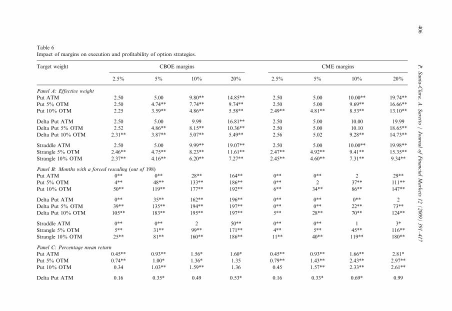
The analysis is conducted considering different target weights from 2.5% to 20% andthe results are reported in Table 6. Empirical distributions for the quantity of interest areobtained through bootstrapping. Panel A tabulates effective weights for each strategy. The

14The investment opportunity set includes the risk-free rate and the option strategy. One possibility would be to

include the market portfolio. We analyze this case in Section 5.

ARTIC

LEIN

PRES

S

Table 6

Impact of margins on execution and profitability of option strategies.

Target weight CBOE margins CME margins

2.5% 5% 10% 20% 2.5% 5% 10% 20%

Panel A: Effective weight

Put ATM 2.50 5.00 9.80** 14.85** 2.50 5.00 10.00** 19.74**

Put 5% OTM 2.50 4.74** 7.74** 9.74** 2.50 5.00 9.69** 16.66**

Put 10% OTM 2.25 3.59** 4.86** 5.58** 2.49** 4.81** 8.53** 13.10**

Delta Put ATM 2.50 5.00 9.99 16.81** 2.50 5.00 10.00 19.99

Delta Put 5% OTM 2.52 4.86** 8.15** 10.36** 2.50 5.00 10.10 18.65**

Delta Put 10% OTM 2.31** 3.87** 5.07** 5.49** 2.56 5.02 9.28** 14.73**

Straddle ATM 2.50 5.00 9.99** 19.07** 2.50 5.00 10.00** 19.98**

Strangle 5% OTM 2.46** 4.75** 8.23** 11.61** 2.47** 4.92** 9.41** 15.35**

Strangle 10% OTM 2.37** 4.16** 6.20** 7.27** 2.45** 4.60** 7.31** 9.34**

Panel B: Months with a forced rescaling (out of 198)

Put ATM 0** 0** 28** 164** 0** 0** 2 29**

Put 5% OTM 4** 48** 133** 186** 0** 2 37** 111**

Put 10% OTM 50** 119** 177** 192** 6** 34** 86** 147**

Delta Put ATM 0** 35** 162** 196** 0** 0** 0** 2

Delta Put 5% OTM 39** 135** 194** 197** 0** 0** 22** 73**

Delta Put 10% OTM 105** 183** 195** 197** 5** 28** 70** 124**

Straddle ATM 0** 0** 2 50** 0** 0** 1 3*

Strangle 5% OTM 5** 31** 99** 171** 4** 5** 45** 116**

Strangle 10% OTM 25** 81** 160** 186** 11** 40** 119** 180**

Panel C: Percentage mean return

Put ATM 0.45** 0.93** 1.56* 1.60* 0.45** 0.93** 1.66** 2.81*

Put 5% OTM 0.74** 1.00* 1.36* 1.35 0.79** 1.43** 2.43** 2.97**

Put 10% OTM 0.34 1.03** 1.59** 1.36 0.45 1.57** 2.33** 2.61**

Delta Put ATM 0.16 0.35* 0.49 0.53* 0.16 0.33* 0.69* 0.99

P.

Sa

nta

-Cla

ra,

A.

Sa

retto/

Jo

urn

al

of

Fin

an

cial

Ma

rkets

12

(2

00

9)

39

1–

41

7406

ARTIC

LEIN

PRES

SDelta Put 5% OTM 0.48** 0.63** 0.71** 0.73** 0.53** 1.08** 1.39 1.95

Delta Put 10% OTM 0.34 0.46 0.51 0.53 0.14 0.25 1.53** 0.31

Straddle ATM 0.17* 0.36** 0.52 0.97 0.17* 0.36** 0.52 1.00

Strangle 5% OTM 0.55** 0.98** 0.94 0.99 0.56** 1.13** 1.66** 1.97**

Strangle 10% OTM 0.80** 1.07** 1.26 1.75** 0.87** 1.62** 1.78** 2.37**

Panel D: Sharpe ratio

Put ATM 0.19** 0.20** 0.14* 0.12* 0.19** 0.20** 0.15** 0.13*

Put 5% OTM 0.24** 0.13* 0.15* 0.12 0.26** 0.18** 0.18** 0.16**

Put 10% OTM 0.04 0.18** 0.25** 0.12 0.05 0.22** 0.19** 0.16**

Delta Put ATM 0.12 0.14* 0.12 0.13* 0.12 0.12* 0.13* 0.06

Delta Put 5% OTM 0.23** 0.16** 0.17** 0.18** 0.25** 0.25** 0.12 0.11

Delta Put 10% OTM 0.08 0.09 0.10 0.10 0.02 0.01 0.17** 0.01

Straddle ATM 0.14* 0.15** 0.07 0.07 0.14* 0.15** 0.07 0.07

Strangle 5% OTM 0.29** 0.25** 0.09 0.10 0.29** 0.29** 0.16** 0.16**

Strangle 10% OTM 0.35** 0.24** 0.12 0.19** 0.38** 0.36** 0.16** 0.23**

Panel E: Leland alpha

Put ATM 0.09 0.20 �0.16 �0.58 0.09 0.20 �0.11 �0.65

Put 5% OTM 0.25 �0.19 �0.13 �0.51 0.30 0.23 0.35 0.08

Put 10% OTM �0.77 0.16 0.61* �0.29 �0.68 0.53 0.46 0.11

Delta Put ATM 0.03 0.11 0.07 0.12 0.03 0.08 0.19 �0.62

Delta Put 5% OTM 0.30 0.26 0.31 0.33 0.35* 0.73* 0.22 0.13

Delta Put 10% OTM �0.05 �0.02 0.03 0.05 �0.70 �1.35 0.89 �2.40

Straddle ATM 0.08 0.19 �0.12 �0.27 0.08 0.19 �0.11 �0.30

Strangle 5% OTM 0.45** 0.77** 0.12 0.24 0.45** 0.92** 0.86 1.27

Strangle 10% OTM 0.80** 1.09** 1.25 1.83 0.86** 1.61** 1.69 2.36*

Panel F: MPPM

Put ATM �0.01 0.01 �6.67 �6.72 �0.01 0.01 �6.67 �6.93

Put 5% OTM 0.01 �2.03 �0.45 �2.68 0.02 �1.99 �6.68 �8.72**

Put 10% OTM �6.67 �0.02 0.02 �6.67 �6.67 �0.06 �6.73 �6.78

Delta Put ATM �0.04** �0.03 �0.04 �0.03 �0.04** �0.03 �0.04 �6.69

Delta Put 5% OTM �0.01 �0.02 �0.02 �0.02 �0.00 0.02 �6.69 �6.95*

Delta Put 10% OTM �0.09 �0.16 �0.16 �0.16 �6.69 �6.66 �0.16 �9.82**

P.

Sa

nta

-Cla

ra,

A.

Sa

retto/

Jo

urn

al

of

Fin

an

cial

Ma

rkets

12

(2

00

9)

39

1–

41

7407

ARTIC

LEIN

PRES

STable 6 (continued )


2.5% 5% 10% 20% 2.5% 5% 10% 20%

Straddle ATM �0.04** �0.02 �1.47 �6.67 �0.04** �0.02 �1.47 �6.68

Strangle 5% OTM 0.00 0.03 �6.67 �0.88 0.01 0.05 �6.65 �0.30

Strangle 10% OTM 0.03 0.03 �6.68 �1.33 0.04 0.09 �6.67 �1.67

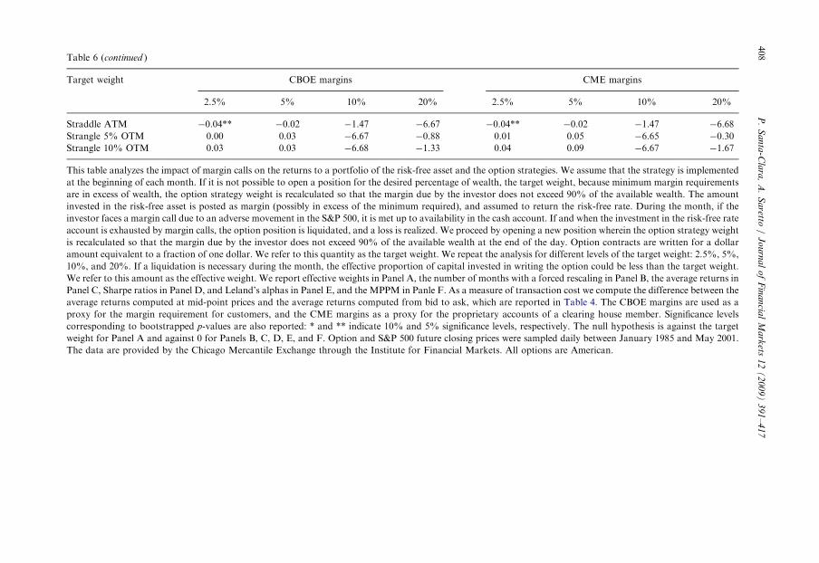
This table analyzes the impact of margin calls on the returns to a portfolio of the risk-free asset and the option strategies. We assume that the strategy is implemented

at the beginning of each month. If it is not possible to open a position for the desired percentage of wealth, the target weight, because minimum margin requirements

are in excess of wealth, the option strategy weight is recalculated so that the margin due by the investor does not exceed 90% of the available wealth. The amount

invested in the risk-free asset is posted as margin (possibly in excess of the minimum required), and assumed to return the risk-free rate. During the month, if the

investor faces a margin call due to an adverse movement in the S&P 500, it is met up to availability in the cash account. If and when the investment in the risk-free rate

account is exhausted by margin calls, the option position is liquidated, and a loss is realized. We proceed by opening a new position wherein the option strategy weight

is recalculated so that the margin due by the investor does not exceed 90% of the available wealth at the end of the day. Option contracts are written for a dollar

amount equivalent to a fraction of one dollar. We refer to this quantity as the target weight. We repeat the analysis for different levels of the target weight: 2.5%, 5%,

10%, and 20%. If a liquidation is necessary during the month, the effective proportion of capital invested in writing the option could be less than the target weight.

We refer to this amount as the effective weight. We report effective weights in Panel A, the number of months with a forced rescaling in Panel B, the average returns in

Panel C, Sharpe ratios in Panel D, and Leland’s alphas in Panel E, and the MPPM in Panle F. As a measure of transaction cost we compute the difference between the

average returns computed at mid-point prices and the average returns computed from bid to ask, which are reported in Table 4. The CBOE margins are used as a

proxy for the margin requirement for customers, and the CME margins as a proxy for the proprietary accounts of a clearing house member. Significance levels

corresponding to bootstrapped p-values are also reported: * and ** indicate 10% and 5% significance levels, respectively. The null hypothesis is against the target

weight for Panel A and against 0 for Panels B, C, D, E, and F. Option and S&P 500 future closing prices were sampled daily between January 1985 and May 2001.

The data are provided by the Chicago Mercantile Exchange through the Institute for Financial Markets. All options are American.

P.

Sa

nta

-Cla

ra,

A.

Sa

retto/

Jo

urn

al

of

Fin

an

cial

Ma

rkets

12

(2

00

9)

39

1–

41

7408


results reported in the table confirm our conjecture: if the target weight is small, 2.5% ofcapital, the difference between target and effective weight is small. For target weightslarger than 2.5%, as is also suggested by the analysis of the haircut ratios in Table 5, theimpact of margins is greater for lower moneyness options. If the target weight is high, 20%or more, the effect of margins on the allocation of capital to option strategies can beeconomically very large. On the one hand, for ATM options margins have little impact onstrategy execution. For example, if the target weight is 20%, in the case of the far ATMstraddle, the difference between the target and the effective weight is 0.83% for CBOEcustomers and 0.02% for CME members. On the other hand, the impact is quite largewhen OTM options are considered. For example, if the target weight is 20%, in the case ofthe 5% OTM put, the difference between target and effective weight is 10.2% for CBOEcustomers and 3.4% for CME members. That represents a 50% and 20% potential profitreduction, respectively.

We formally confirm the result by estimating the correlation between the level of thetarget weight and the difference between the target and the effective weight. First, wecompute the Spearman rank correlation coefficient. The estimate of the correlationcoefficient is equal to 0.67 and is highly statistically significant. Second, since themagnitude of the difference between the target and the effective weight varies acrossdifferent strategies, we estimate a linear regression, of target weight on the difference,which allows to control for a variety of fixed effects: puts versus hedges versuscombinations, CBOE margins versus CME margins. After controlling for thesecharacteristics, the estimated coefficient on the target weight is equal to 0.345 and ishighly statistically significant (t-stat of 6.1).

In Panel B of Table 6, we report the number of months during which the investor isunable to cover the initial or the maintenance requirement corresponding to the targetweight. To simplify notation we refer to all those cases as ‘‘rescalings.’’ The pattern issimilar to what suggested by the results in Panel A: failures to comply with therequirements are more numerous for low moneyness strategies. The number of rescalings isquite high: if the target weight is equal to 20%, OTM strategies endure a rescaling inalmost every month of the sample.

4.2. Impact on profitability

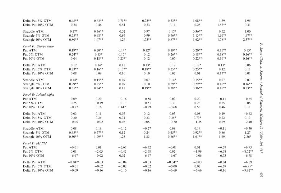
Margins have an effect on the profitability of the strategies through two channels. First,a positive difference between target and effective weight represents an opportunity cost tothe investor in the form of missed profits that originate from the fact that capital has to beallocated to the margin account instead of to trading options. Second, since margincalls happen when the market is moving against the investor’s position in the option(underlying price decreases or volatility increases), liquidations will also have the effect offorcing the investor to realize losses. In Panel C of Table 6, we report the average strategyreturns. A higher target weight leads to a larger average return. However, the averagereturn corresponding to a target weight of 10% is not twice as large as the averagereturn of a 5% exposure. That is especially true for those strategies for which marginsmatter the most. For example, the average return of the 10% OTM strangle for a CMEmember investor rises from 1.78% to 2.37% when the portfolio weight increases from 10%to 20%.


We also compute performance measures that take some dimension of risk into account.We report Sharpe ratios in Panel D of Table 6,15 Leland’s alpha in Panel E,16 and theMPPM of Ingersoll et al. (2007) in Panel F.17

With very few exceptions, the performance measures decrease when moving from asmaller to a larger option portfolio weight. For example, the Sharpe ratio corresponding toa target weight of 20% is lower than the Sharpe ratio corresponding to a target weight of2.5% for approximately two-thirds of the strategies. A similar pattern is observed for theother profitability measures: the percentage is about 70% for the Leland’s alpha and about90% for the MPPM. For example, let’s consider the ATM straddle, which is an optionstrategy which performance is found to be most problematic in the literature (see, forexample, Bates, 2007). When going from a 2.5% to a 20% target weight, the SR decreasesfrom 0.14 to 0.07, the Leland alpha from 0:08 to� 0:27, and the MPPM from�0:04 to� 6:67.Some of these performance measures are reported in other studies: for example

Bondarenko (2003), Coval and Shumway (2001), Jones (2006), and Driessen andMaenhout (2007). These studies analyze strategy returns as if there were no marginrequirements. Let’s consider for example the case of the Leland model. The abovementioned studies find that alphas for put option strategies are really large and statisticallysignificant.18 We find a different result because we consider returns after margins are takeninto account. Examining the relation between the allocation sought by the investor and thesize and significance of the alphas we notice that a larger target weight usually implies alower alpha and a lower significance level. The result is due to the fact that the covarianceof the strategy returns with the market increases with the strategy exposure, leading tolower or zero alphas. The covariance increases because the return on the strategy isnegatively affected by the inability of the investor to cover margin calls, which tend tohappen when the market return is negative.To summarize, a rise in volatility and/or a drop in the underlying price causes an

increase in the margin requirement. If investors do not have easy access to capital, anincrease in maintenance margins severely affects the execution of option strategies thatinvolve writing options. The investor is forced to realize losses, even if the strategy couldultimately lead to a positive return. The profitability of the strategies is therefore affected.

5. Impact of margin requirements: three assets

In the previous section, we show that the amount of capital that must be devoted tomargins is high relative to the price of an option contract. The conclusion that we can drawis that the opportunity cost related to maintaining margins is the key in trading/writingoptions. In the economic setting described in Section 4, the opportunity cost arises because

15Note that, since the portfolio is short in options and long in the risk-free rate account for different amounts,

the strategy Sharpe ratios will not be exactly equal to those reported in Table 2.16Results for alpha derived from the CAPM and the Fama and French (1993) three factors model are very

similar and can be obtained from the authors upon request.17Ingersoll et al. (2007) derive a performance measure that cannot be manipulated by information-unrelated

trades: MPPM ¼ ð1=ð1� rÞDtÞ logðð1=TÞPT

t¼1 ½ð1þ rtÞ=ð1þ rf tÞ�1�rÞ, where r is a coefficient that should be

chosen to make holding the benchmark optimal. We set it equal to 2 as suggested by the authors. The

corresponding MPPM for the market portfolio is then 0.18Driessen and Maenhout (2007) include CBOE margins in parts of their analysis.


capital has to be invested in the margin account with a return equal to the short-terminterest rate (typically the rate on a Treasury bill).

In this section, we modify the economic setting of Section 4 in two ways. First, weinclude S&P 500 futures in the investment opportunity set. Second, we consider differentpossibilities as to what exposure the investor can take in the futures: the investor can take apositive exposure in an attempt to increase the return of the margin account; or theinvestor can take a negative exposure in an attempt to reduce the margin by taking a hedgein the underlying.

Therefore, with this analysis, we study whether the inclusion of a third asset can improveon the ability of the investor to trade options by reducing the opportunity cost related tomaintaining margins. In other words, we are seeking further verification that margins dohave an impact on trading options even when the investor is allowed to try to minimize theopportunity cost of maintaining the margin account by using as collateral an asset that hasa higher average return then the risk-free rate.

As noted above, we study several scenarios that comprise the instance in which theinvestor takes a short position in one futures contract for each written option contract, inwhich case the put options are completely covered. We refer to this case as completecoverage. For symmetry we also analyze the case where the investor takes a long positionin one futures contract for each written option contract (negative coverage). Therefore, inour experiment, the possible option portfolio weights vary between �2:5% and �20% (asbefore), while the coverage ratio varies between 1 (the put option is completely covered)and �1 (long position in the underlying for an amount equivalent to a full cover) withincrements of 0.5. The results for exact delta-hedged strategies are contained in theprevious sections. For example, let’s consider the case of an investor that writes 10 putoption contracts. A coverage ratio of 0.5 would imply covering the position with fivefutures contracts, while a coverage ratio of �0:5 would imply a long position of five futurescontract. Note that the positions are all relative to an initial investment of $1. Scaling upthat amount affects the number of contracts but does not change the returns.

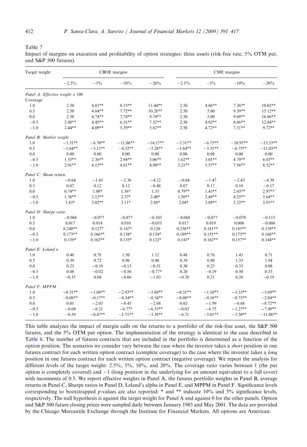
We report the results of the analysis for the 5% OTM put option strategy in Table 7.19

5.1. Impact on execution

As we can see from Panel A of the Table 7, the margins have an impact on the executionof option strategies whether the futures is traded or not. Across different coverage ratios,the difference between the target and the effective option weight is bigger in the cases whenthe investor seeks to write options more aggressively (higher target weights). Across optiontarget weights, positive or negative coverage does not increase the effective option weight.For the CME margining system, which is based on projected losses from the totalportfolio, the maximum exposure to options is obtained with zero coverage. The result isdue to the fact that the CME margins take into account the correlation between the optionand the underlying payoff. The very large exposure to the underlying, reported in Panel B,has in fact a pervasive effect on the capital that is available to cover margins. The hedge(positive coverage) comes at a great cost: the large negative position in the underlying thatis necessary to cover the option generates enough losses to significantly decrease the capital

19Results for all the other strategies are not reported to limit the number of tables but they are available upon

request.

ARTICLE IN PRESS

Table 7

Impact of margins on execution and profitability of option strategies: three assets (risk-free rate, 5% OTM put,

and S&P 500 futures).


�2.5% �5% �10% �20% �2.5% �5% �10% �20%

Panel A: Effective weight� 100

Coverage

1.0 2.50 4.85** 8.15** 11.44** 2.50 4.66** 7.36** 10.02**

0.5 2.50 4.84** 7.72** 10.28** 2.50 5.00 9.39** 15.12**

0.0 2.50 4.74** 7.74** 9.74** 2.50 5.00 9.69** 16.66**

�0.5 2.48** 4.45** 6.51** 7.32** 2.50 4.92** 8.66** 12.84**

�1.0 2.44** 4.09** 5.39** 5.82** 2.50 4.72** 7.51** 9.72**

Panel B: Market weight

1.0 �3.31** �6.70** �11.06** �14.17** �3.31** �6.75** �10.97** �13.53**

0.5 �1.64** �3.11** �4.52** �5.28** �1.64** �3.31** �6.75** �11.03**

0.0 0.00 0.00 0.00 0.00 0.00 0.00 0.00 0.00

�0.5 1.55** 2.36** 2.94** 3.06** 1.62** 3.01** 4.79** 6.03**

�1.0 2.91** 4.15** 4.81** 4.90** 3.21** 5.57** 7.56** 8.52**

Panel C: Mean return

1.0 �0.64 �1.45 �2.36 �4.12 .�0.64 �1.47 �2.43 �4.39

0.5 0.07 0.12 0.12 �0.48 0.07 0.17 0.10 �0.17

0.0 0.74** 1.00* 1.36* 1.35 0.79** 1.43** 2.43** 2.97**

�0.5 1.38** 2.12** 2.37* 2.40* 1.50** 2.49** 4.25** 5.64**

�1.0 1.85* 3.02** 3.11* 2.88* 2.04* 3.89** 5.32** 5.91**

Panel D: Sharpe ratio

1.0 �0.068 �0.077 �0.077 �0.103 �0.068 �0.077 �0.079 �0.115

0.5 0.017 0.014 0.010 �0.033 0.017 0.019 0.006 �0.006

0.0 0.240** 0.127* 0.147* 0.120 0.256** 0.181** 0.185** 0.159**

�0.5 0.173** 0.166** 0.138* 0.130* 0.189** 0.151** 0.175** 0.168**

�1.0 0.139* 0.162** 0.135* 0.122* 0.141* 0.162** 0.157** 0.144**

Panel E: Leland a1.0 0.48 0.78 1.50 1.12 0.48 0.76 1.45 0.71

0.5 0.39 0.72 0.96 0.40 0.39 0.80 1.35 1.94

0.0 0.25 �0.19 �0.13 �0.51 0.30 0.23 0.35 0.08

�0.5 0.08 �0.02 �0.56 �0.77* 0.20 �0.19 0.50 0.53

�1.0 �0.31 0.04 �0.66 �1.03 �0.28 0.21 0.26 �0.19

Panel F: MPPM

1.0 �0.31** �1.04** �2.93** �5.88** �0.31** �1.10** �3.33** �5.69**

0.5 �0.08** �0.17** �0.34** �0.54** �0.08** �0.18** �0.73** �2.84**

0.0 0.01 �2.03 �0.45 �2.68 0.02 �1.99 �6.68 �8.72**

�0.5 �0.04 �0.21 �6.77* �6.53** �0.03 �6.75 �1.27** �7.49**

�1.0 �0.59 �0.47** �1.71** �3.38** �6.71 �3.01** �3.50** �11.06**

This table analyzes the impact of margin calls on the returns to a portfolio of the risk-free asset, the S&P 500

futures, and the 5% OTM put option. The implementation of the strategy is identical to the case described in

Table 6. The number of futures contracts that are included in the portfolio is determined as a function of the

option position. The scenarios we consider vary between the case where the investor takes a short position in one

futures contract for each written option contract (complete coverage) to the case where the investor takes a long

position in one futures contract for each written option contract (negative coverage). We repeat the analysis for

different levels of the target weight: 2.5%, 5%, 10%, and 20%. The coverage ratio varies between 1 (the put

option is completely covered) and �1 (long position in the underlying for an amount equivalent to a full cover)

with increments of 0.5. We report effective weights in Panel A, the futures portfolio weights in Panel B, average

returns in Panel C, Sharpe ratios in Panel D, Leland’s alpha in Panel E, and MPPM in Panel F. Significance levels

corresponding to bootstrapped p-values are also reported: * and ** indicate 10% and 5% significance levels,

respectively. The null hypothesis is against the target weight for Panel A and against 0 for the other panels. Option

and S&P 500 future closing prices were sampled daily between January 1985 and May 2001. The data are provided

by the Chicago Mercantile Exchange through the Institute for Financial Markets. All options are American.



that is available to the investor. On the other hand, the long positions in the underlying(negative coverage) produce losses precisely when the option position is losing money(market drops), thus accentuating the portfolio down-side risk, and hence increasingmargins.

5.2. Impact on profitability

Examining the profitability measures, we note that the best performance is oftenobtained with zero coverage and for small target option weight. The sign and magnitude ofthe average returns is inversely related to the coverage ratio: positive coverage (shortpositions in the futures) produces negative average returns, while negative coverage isassociated with positive average returns. When margins are taken into account, perfectcoverage of the option is quite expensive: for example, full coverage of a �10% optionposition produces an average return of �2:43% per month. This is essentially due to thefact that the futures contracts necessary to implement the cover correspond to an exposureto the underlying of �11 times of the available capital. (Such an exposure can only beobtained through futures.)

Considering the combinations that produce positive returns, the Sharpe ratios tend todecrease going from zero to negative coverage. Ingersoll et al. (2007) show that Sharperatios can be easily manipulated by using options. The measure they propose (MPPM) isespecially adequate to evaluate strategy performance in this setting wherein options arepaired with positions in the S&P 500. The MPPM is in fact calibrated so that a portfoliothat would be entirely invested in the S&P 500 would have a score equal to zero. As we cansee from Panel F of Table 7, MPPM is decreasing with the option weight and the absolutevalue of the coverage. The measure is positive or close to zero only for a very smallposition (2.5% in the option and zero coverage) in the option and is negative and large forextreme positions.

In summary, an investor is better off trading a smaller number of option contracts as theperformance tends to deteriorate when larger exposures to the options are sought. Resultsfor all the other strategies (puts, straddles, and strangles) are similar both quantitativelyand qualitatively.

5.2.1. Regression approach

In order to gather an overall perspective we frame the analysis in the context of a linearregression. We pool the estimated performance measures for each pair of option weightsand coverage ratios for the six basic strategies (three naked puts and the straddle and thetwo strangles).

We run a panel regression of the performance measure on the option target weight (wop)and the coverage ratio (cover) controlling for various fixed effects: CBOE versus CME, putversus combination, and the three levels of moneyness. We run the following regression:

X ¼ aþ b wop þ g coverþ �,

where X ¼ fw�op; SR; Leland a; MPPMg. w�op is defined as the difference between theeffective and the target weight. For convenience of interpretation, we use the absolutevalue of wop as the independent variable, so that a larger number represents a larger optionportfolio weight.

ARTICLE IN PRESS

Table 8

Impact of margins on execution and profitability of option strategies, linear regression.

w�op SR LEL MPPM

wop �0.474 �0.195 �0.261 �23.623

(�15.25) (�2.52) (�3.90) (�10.42)

cover 0.005 �0.155 0.019 0.999

(2.28) (�24.47) (3.29) (4.93)

R2 0.692 0.631 0.182 0.431

We pool the estimated performance measures for each pair of option weights and coverage ratios for the six basic

strategies (three naked puts, the straddle, and two strangles). We run a fixed effect panel regression in which we

control for various characteristic: CBOE versus CME, put versus combination, and the three levels of moneyness:

X ¼ aþ bwop þ g coverþ �,

where X ¼ fw�op; SR; Leland a ðLELÞ; MPPMg. w�op is defined as the difference between the effective and the

target weight. For convenience of interpretation, we use the absolute value of the target weight wop as the

independent variable, so that a larger number represents a larger option portfolio weight. cover is the coverage

ratio. Since there are twenty combinations of option weight and coverage ratios for each strategy, and there are six

basic strategies for each of the two margining systems, each regression is based on a sample of 240 observations.

Clustered and heteroskedasticity consistent standard errors are used to compute the t-statistics, which are

reported in parenthesis. Constants and the fixed-effect dummies are not reported.


Since there are 20 combinations of option weight and coverage ratios for each strategyand there are six basic strategies for each of the two margining systems, each regression isbased on a sample of 240 observations. Our null hypothesis (margins do not have anyimpact) is that the strategy performance improves or does not deteriorate by increasing theoption exposure (wop). A statistically significant negative estimated coefficient ðbÞ thusleads to rejection of the null hypothesis. The results are reported in Table 8.The estimated slope coefficients of the option portfolio weight ðwopÞ are all negative. The

results of this analysis are strongly supportive of our conjecture: increasing the portfolioexposure to the option and controlling for the level of coverage leads to a deterioration ofthe portfolio profitability and to a bigger difference between effective and target weight.The t-statistics confirm that the estimates are negative at conventional significance levels.

6. Conclusion

Previous studies report unusually high returns to option strategies that involve writingput options. The contribution of this paper is to show that the returns realizable byinvestors subject to the margining systems are not as large as previously documented. Weshow that, if margins are taken into account, part of the ‘‘un-margined’’ returns is notavailable to investors. Therefore, while volatility and jump risk premia are priced intooption prices, limits to arbitrage, represented by transaction costs and marginrequirements, might blunt the effectiveness of option markets for risk sharing amonginvestors.The fact that liquidity in the option market has traditionally been supplied by market-

makers (Bates, 2001; Bollen and Whaley, 2004; Garleanu et al., 2005) provides theeconomic rationale for the importance of margin requirements in explaining option prices.


In Garleanu et al. (2005), high prices are driven by market-makers who charge a premiumbecause they are unable to completely hedge away the risk involved with an unbalancedinventory. We argue that, despite being attracted by high prices, other investors are limitedfrom supplying liquidity to the market by the fact that they have to maintain margins.Lack of liquidity allows high prices to persist in the market. Although we do not examineflights to liquidity, the argument that is proposed in this study is similar to that presentedby Garleanu and Pedersen (2007) and Mitchell et al. (2007), wherein internal riskmanagement causes market players to reduce their participation to the market. Weconsider a form of ‘‘external’’ risk management imposed by the option exchanges: marginrequirements.

Acknowledgments

We thank Dave Denis, Stephen Figlewski, Laura Frieder, Jun Liu, Francis Longstaff,John Mcconnell, George Skiadopoulous, Walter Torous and seminar participants at theSpring 2005 NBER Behavioral Finance meeting, the 2006 EFA meeting in Zurich, PurdueUniversity, UCLA, and especially an anonymous referee for valuable suggestions.

References

Bakshi, G., Cao, C., Chen, Z., 1997. Empirical performance of alternative option pricing models. Journal of

Finance 52, 2003–2049.

Bakshi, G., Kapadia, N., 2003. Delta-hedged gains and the negative market volatility risk premium. Review of

Financial Studies 16, 527–566.

Bates, D.S., 1996. Jumps and stochastic volatility: exchange rate processes implicit in Deutshe Mark options.

Review of Financial Studies 1, 69–107.

Bates, D.S., 2000. Post-’87 crash fear in the S&P 500 futures option market. Journal of Econometrics 94, 181–238.

Bates, D.S., 2001. The market for crash risk. Working Paper, University of Iowa.

Bates, D.S., 2003. Empirical option pricing: a retrospective. Journal of Econometrics 116, 387–404.

Battalio, R., Stultz, P., 2006. Options and the bubble. Journal of Finance 61, 2071–2102.

Bensaid, B., Lesne, J.-P., Pages, H., Scheinkman, J., 1992. Derivative asset pricing with transaction costs.

Mathematical Finance 2, 63–86.

Benzoni, L., 2002. Pricing options under stochastic volatility: an empirical investigation. Working Paper.

Benzoni, L., Collin-Dufresne, P., Goldstein, R.S., 2005. Can standard preferences explain the prices of out-of-the-

money S&P 500 put options? Working Paper.

Black, F., 1976. The pricing of commodity contracts. Journal of Financial Economics 3, 167–179.

Bollen, N.P., Whaley, R.E., 2004. Does net buying pressure affect the shape of implied volatility functions?

Journal of Finance 59, 711–753.

Bondarenko, O., 2003. Why are put options so expensive? Working Paper.

Broadie, M., Chernov, M., Johannes, M.S., 2006. Model specification and risk premia: evidence from futures

options. Journal of Finance 62, 1453–1490.

Broadie, M., Chernov, M., Johannes, M.S., 2007. Understanding index option returns. Working Paper.

Brunnermeier, M.K., Pedersen, L.H., 2008. Market liquidity and funding liquidity. Review of Financial Studies,

forthcoming.

Buraschi, A., Alexei, J., 2006. Model uncertainty and option markets with heterogeneous beliefs. Journal of

Finance 61, 2841–2897.

Buraschi, A., Jackwerth, J., 2001. The price of a smile: hedging and spanning in option markets. Review of

Financial Studies 14, 492–527.

Chernov, M., Gallant, R., Ghysels, E., Tauchen, G., 2003. Alternative models for stock price dynamics. Journal

of Econometrics 116, 225–257.

Chernov, M., Ghysels, E., 2000. A study towards a unified approach to the joint estimation of objective and risk

neutral measures. Journal of Financial Economics 56, 407–458.


Christensen, B.J., Prabhala, N.R., 1998. The relation between implied and realized volatility. Journal of Financial

Economics 50, 125–150.

Constantinides, G., Jackweth, J.C., Perrakis, S., 2008. Mispricing of S&P 500 options. Review of Financial

Studies, forthcoming.

Constantinides, G., Perrakis, S., 2002. Mispricing of S&P 500 options. Journal of Economic Dynamics & Control

26, 1323–1352.

Constantinides, G., Zariphopoulou, T., 2001. Bounds on derivative prices in an intertemporal setting with

proportional transaction costs and multiple securities. Mathematical Finance 11, 331–346.

Coval, J.D., Shumway, T., 2001. Expected option returns. Journal of Finance 56, 983–1009.

Davison, A.C., Hinkley, D.V., 1997. Bootstrap Methods and their Application. Cambridge University Press,

Cambridge, UK.

Day, T.E., Lewis, C.M., 1992. Stock market volatility and the information content of stock index options. Journal

of Econometrics 52, 267–287.

Driessen, J., Maenhout, P., 2007. A empirical portfolio perspective on option pricing anomalies. Review of

Finance 11, 561–603.

Driessen, J., Maenhout, P., Vilkov, G., 2008. The price of correlation risk: evidence from equity options. Journal

of Finance, forthcoming.

Duarte, J., Lou, X., Sadka, R., 2006. Can liquidity events explain the low-short-interest puzzle? Implications from

the options market. Working Paper.

Duffie, D., Garleanu, N., Pedersen, L.H., 2002. Securities lending, shorting and pricing. Journal of Financial


Eraker, B., 2004. Do stock prices and volatility jumps? Reconciling evidence from spot and option prices. Journal

of Finance 59, 1367–1403.

Eraker, B., Johannes, M., Polson, N., 2003. The impact of jumps in volatility and returns. Journal of Finance 58,

1269–1300.

Fama, E.F., French, K.R., 1993. Common risk factors in the returns on stocks and bonds. Journal of Financial


Figlewski, S., 1989. Options arbitrage in imperfect markets. Journal of Finance 44, 1289–1311.

Garleanu, N., Pedersen, L.H., 2007. Liquidity and risk Management. American Economic Review 97, 193–197.

Garleanu, N., Pedersen, L.H., Poteshman, A.M., 2005. Demand-based option pricing. Working Paper.

George, T.J., Longstaff, F.A., 1993. Bid–ask spreads and trading activity in the S&P 100 index option market.

Journal of Financial and Quantitative Analysis 28, 381–397.

Green, C.T., Figlewski, S., 1999. Market risk and model risk for financial institution writing options. Journal of

Finance 54, 1465–1499.

Han, B., 2008. Investor sentiment and option prices. Review of Financial Studies 21, 387–414.

Heath, D.C., Jarrow, R.A., 1987. Arbitrage, continuous trading, and margin requirements. Journal of Finance 42,

1129–1142.

Ingersoll, J., Spiegel, M., Goetzmann, W., Welch, I., 2007. Portfolio performance manipulation and

manipulation-proof performance measures. Review of Financial Studies 20, 1503–1546.

Jackwerth, J.C., 2000. Recovering risk aversion from option prices and realized returns. Review of Financial

Studies 13, 433–451.

Jackwerth, J.C., Rubistein, M., 1996. Recovering probability distributions from option prices. Journal of Finance

51, 1611–1631.

John, K., Koticha, A., Narayanan, R., Subrahmanyam, M., 2003. Margin rules, informed trading in derivatives,

and price dynamics. Working Paper.

Jones, C.S., 2003. The dynamics of stochastic volatility: evidence from underlying and options markets. Journal of

Econometrics 116, 181–224.

Jones, C.S., 2006. A nonlinear factor analysis of S&P 500 index options returns. Journal of Finance 61,

2325–2363.

Leland, H.E., 1985. Option pricing and replication with transactions costs. Journal of Finance 40, 1283–1301.

Leland, H.E., 1999. Beyond mean-variance: performance measurement in a nonsymmetrical world. Financial

Analysts Journal 55, 27–36.

Liu, J., Longstaff, F., 2004. Losing money on arbitrage: optimal dynamic portfolio choice in markets with

arbitrage opportunities. Review of Financial Studies 17, 611–641.

Liu, J., Pan, J., Wang, T., 2005. An equilibrium model of rare event premia. Review of Financial Studies 18,

131–164.


Mayhew, S., Sarin, A., Shastri, K., 1995. The allocation of informed trading across related markets: an analysis of

the impact of changes in equity-option margin requirements. Journal of Finance 50, 1635–1653.

Mitchell, M., Pedersen, L.H., Pulvino, T., 2007. Slow moving capital. American Economic Review 97, 215–220.

Ofek, E., Richardson, M., Whitelaw, R.F., 2004. Limited arbitrage and short sales restrictions: evidence from the

options market. Journal of Financial Economics 74, 305–342.

Pan, J., 2002. The jump-risk premia implicit in options: evidence from an integrated time-series study. Journal of

Financial Economics 63, 3–50.

Rosenberg, J.V., Engle, R.F., 2002. Empirical pricing kernels. Journal of Financial Economics 64, 341–372.

Rubinstein, M., 1976. The valuation of uncertain income streams and the pricing of options. Bell Journal of


Santa-Clara, P., Yan, S., 2004. Jump and volatility risk and risk premia: a new model and lessons from the S&P

500 options. UCLA Working Paper.

Shleifer, A., Vishny, R.W., 1997. The limits of arbitrage. Journal of Finance 52, 35–55.

Xin, H., Tauchen, G., 2005. The relative contribution of jumps to total variance. Journal of Financial

Econometrics 3, 456–499.

Documents

Option strategies - Universidade Nova de Lisboa