Robotics 1 1

Robotics 1

Kinematic control

Prof. Alessandro De Luca

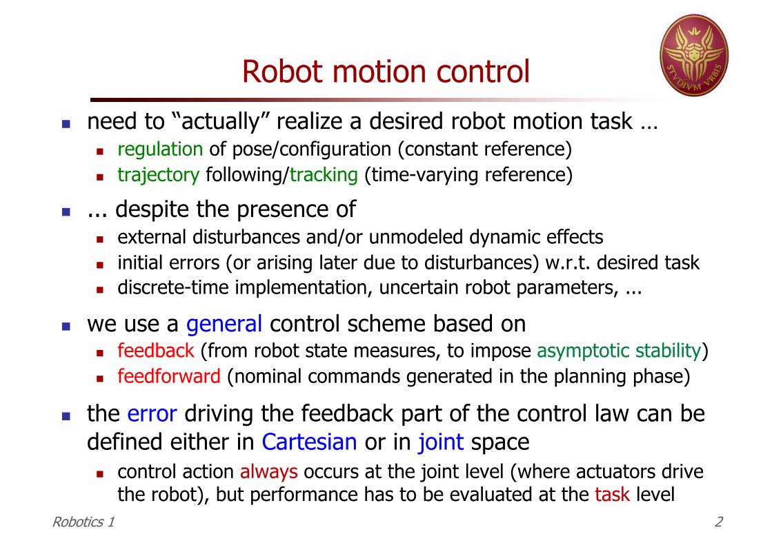
Robot motion controln need to “actually” realize a desired robot motion task …

n regulation of pose/configuration (constant reference)n trajectory following/tracking (time-varying reference)

n ... despite the presence ofn external disturbances and/or unmodeled dynamic effectsn initial errors (or arising later due to disturbances) w.r.t. desired taskn discrete-time implementation, uncertain robot parameters, ...

n we use a general control scheme based onn feedback (from robot state measures, to impose asymptotic stability) n feedforward (nominal commands generated in the planning phase)

n the error driving the feedback part of the control law can be defined either in Cartesian or in joint spacen control action always occurs at the joint level (where actuators drive

the robot), but performance has to be evaluated at the task levelRobotics 1 2

Kinematic control of robots

n a robot is an electro-mechanical system driven by actuating torques produced by the motors

n it is possible, however, to consider a kinematic command (most often, a velocity) as control input to the system...

n ...thanks to the presence of low-level feedback control at the robot joints that allow imposing commanded reference velocities (at least, in the “ideal case”)

n these feedback loops are present in industrial robots within a “closed” control architecture, where users can only specify reference commands of the kinematic type

n in this way, performance can be very satisfactory, provided the desired motion is not too fast and/or does not require large accelerations

Robotics 1 3

An introductory example

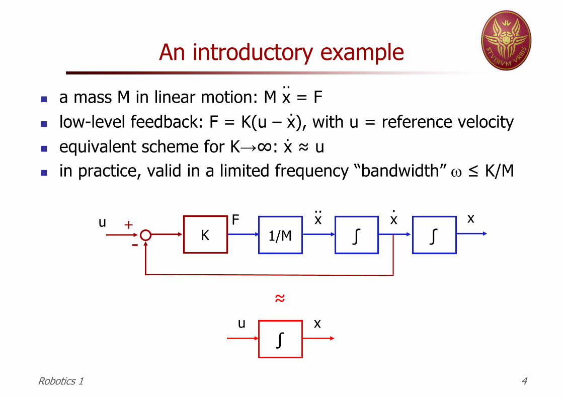
n a mass M in linear motion: M x = Fn low-level feedback: F = K(u – x), with u = reference velocityn equivalent scheme for K→∞: x ≈ un in practice, valid in a limited frequency “bandwidth” w ≤ K/M

..

..

1/M ∫ ∫F xx x

.. .

∫u x

Ku +

-

≈

Robotics 1 4

Frequency responseof the closed-loop system

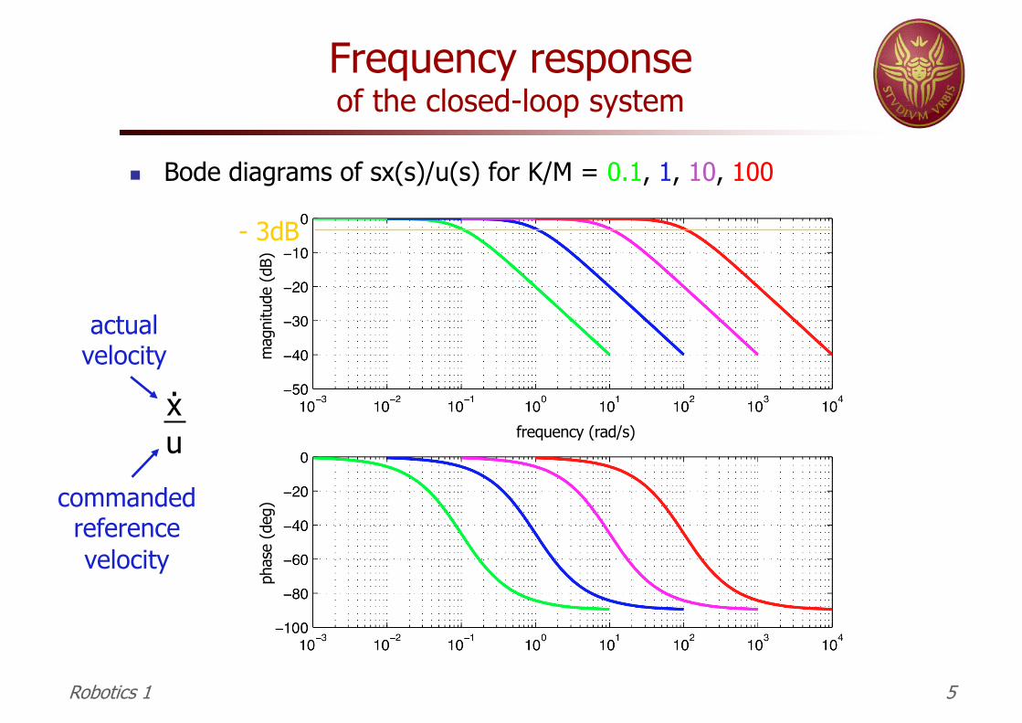
n Bode diagrams of sx(s)/u(s) for K/M = 0.1, 1, 10, 100

xu

.

actualvelocity

commandedreferencevelocity

- 3dB

Robotics 1 5

frequency (rad/s)

phas

e (d

eg)

mag

nitu

de (d

B)

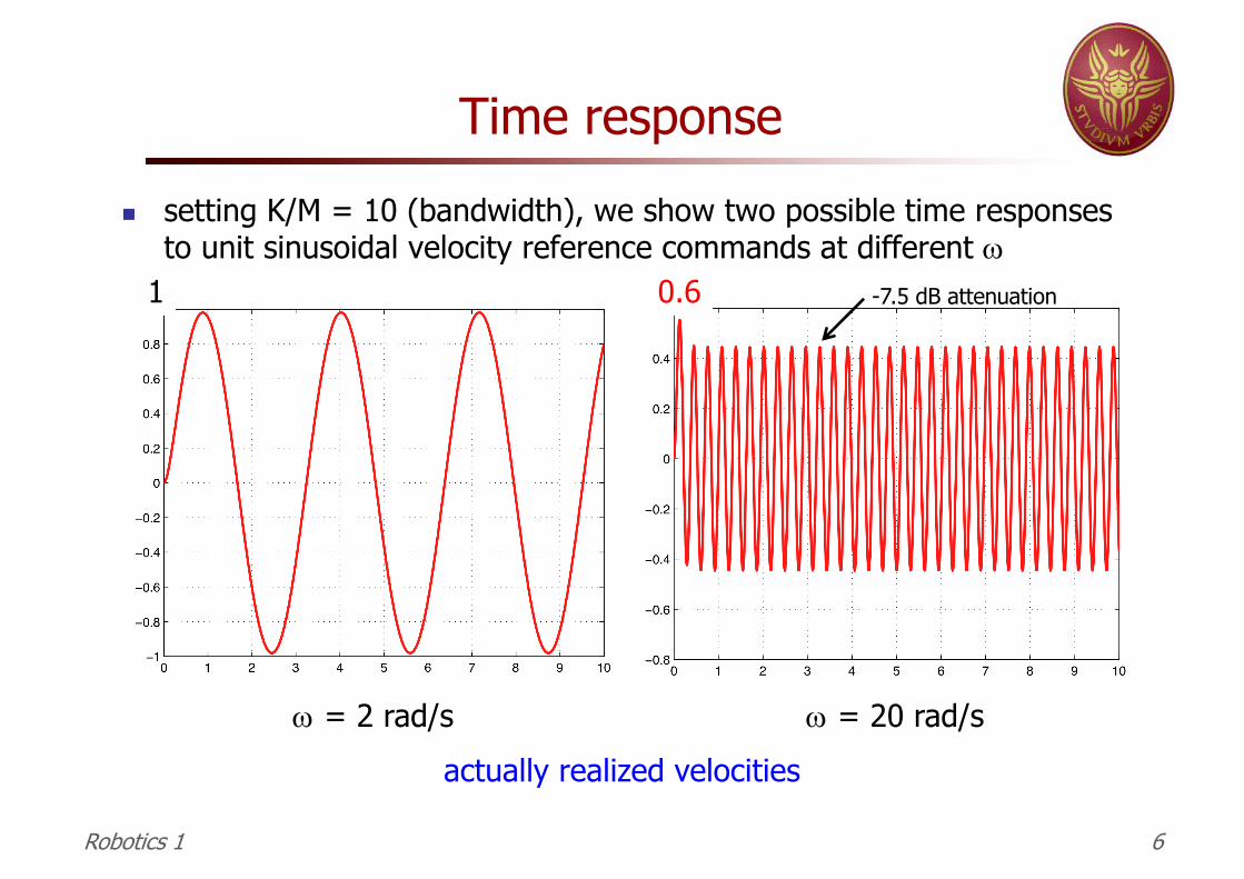
Time responsen setting K/M = 10 (bandwidth), we show two possible time responses

to unit sinusoidal velocity reference commands at different w0.61

w = 2 rad/s w = 20 rad/sactually realized velocities

Robotics 1 6

-7.5 dB attenuation

A more detailed exampleincluding nonlinear dynamics

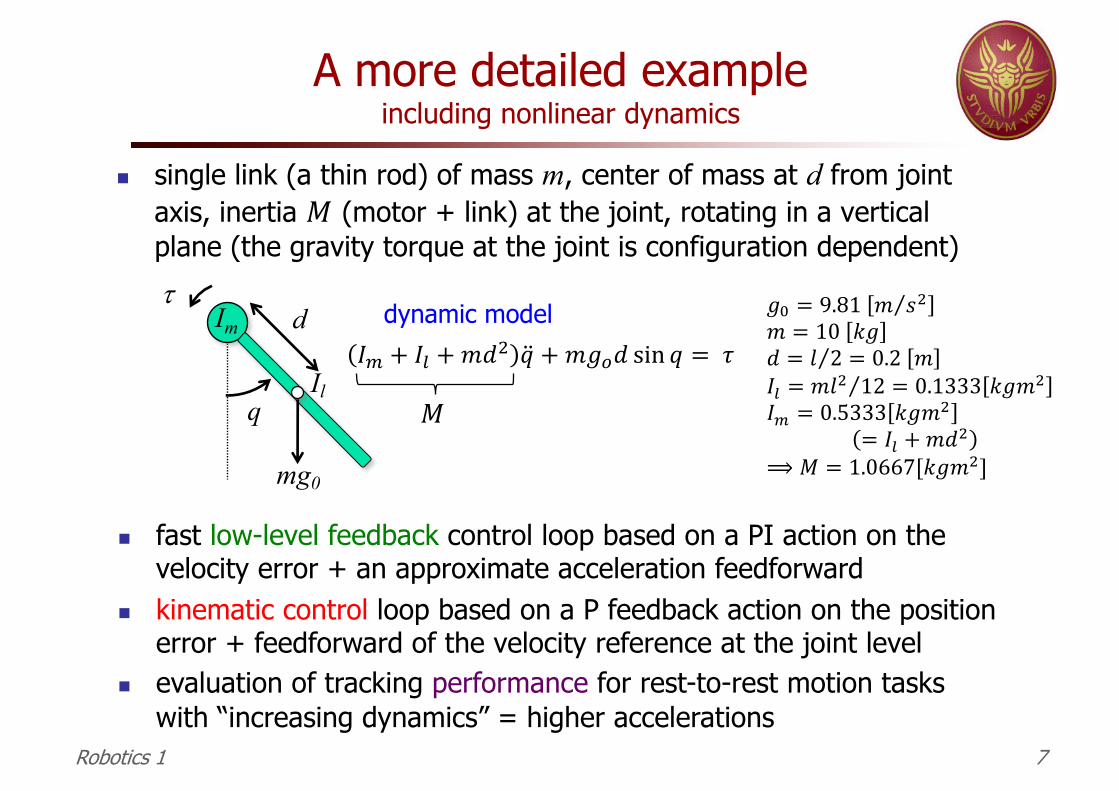
n single link (a thin rod) of mass m, center of mass at d from joint axis, inertia 𝑀 (motor + link) at the joint, rotating in a vertical plane (the gravity torque at the joint is configuration dependent)

Robotics 1 7

𝑀

n fast low-level feedback control loop based on a PI action on the velocity error + an approximate acceleration feedforward

n kinematic control loop based on a P feedback action on the position error + feedforward of the velocity reference at the joint level

n evaluation of tracking performance for rest-to-rest motion tasks with “increasing dynamics” = higher accelerations

q

mg0

dIm

Il

tdynamic model

𝐼# + 𝐼% + 𝑚𝑑( �̈� + 𝑚𝑔,𝑑 sin 𝑞 = 𝜏

𝑔2 = 9.81 ⁄𝑚 𝑠(𝑚 = 10 𝑘𝑔𝑑 = ⁄𝑙 2 = 0.2 𝑚𝐼% = ⁄𝑚𝑙( 12 = 0.1333 𝑘𝑔𝑚(

𝐼# = 0.5333 𝑘𝑔𝑚(

= 𝐼% + 𝑚𝑑(⟹ 𝑀 = 1.0667[𝑘𝑔𝑚(]

A more detailed exampledifferences between the ideal and real case

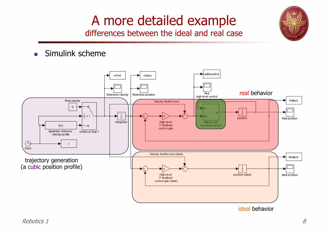
n Simulink scheme

Robotics 1 8

trajectory generation(a cubic position profile)

real behavior

ideal behavior

A more detailed examplerobot with low-level control

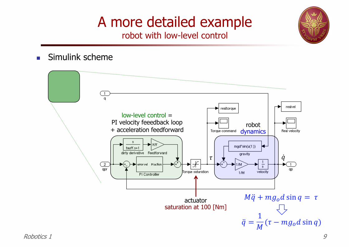
n Simulink scheme

Robotics 1 9

low-level control =PI velocity feeedback loop+ acceleration feedforward

actuatorsaturation at 100 [Nm]

robotdynamics

𝑀�̈� + 𝑚𝑔,𝑑 sin 𝑞 = 𝜏

�̈� =1𝑀 (𝜏 − 𝑚𝑔,𝑑 sin 𝑞)

�̇�𝜏

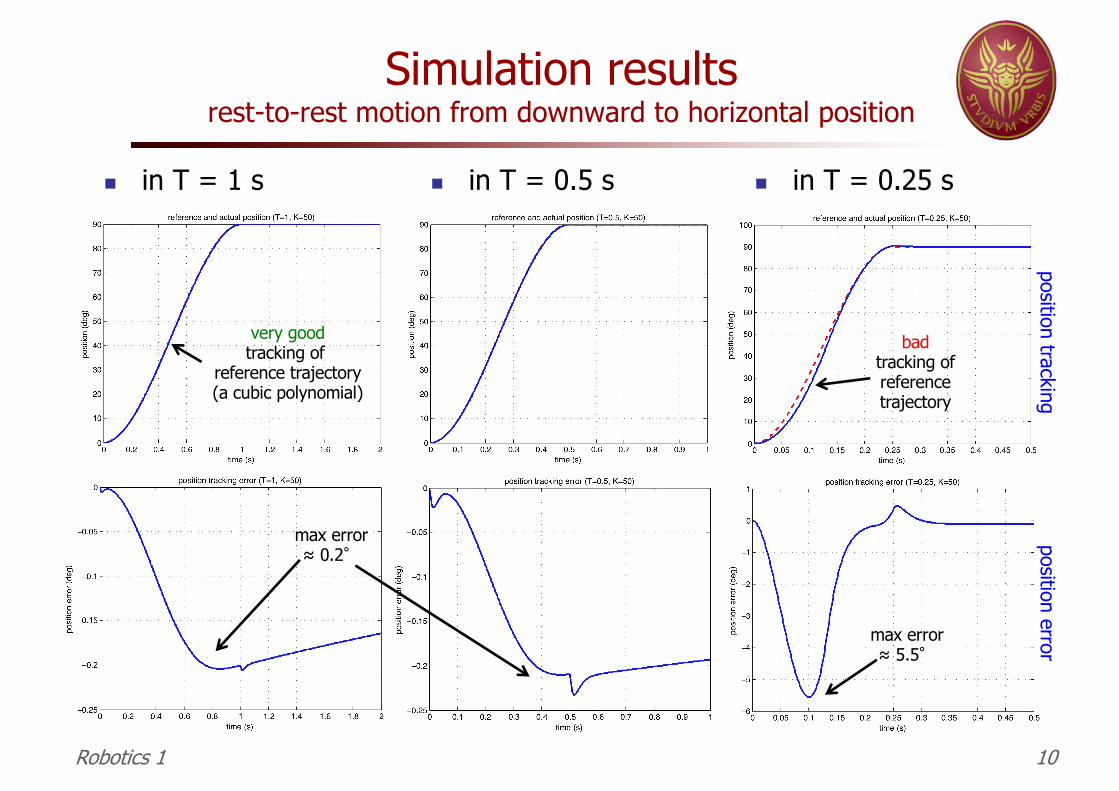
Simulation resultsrest-to-rest motion from downward to horizontal position

n in T = 1 s

Robotics 1 10

n in T = 0.25 s

position trackingposition error

very goodtracking of

reference trajectory(a cubic polynomial)

max error≈ 0.2°

n in T = 0.5 s

badtracking ofreferencetrajectory

max error≈ 5.5°

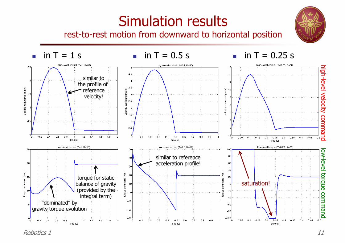
Simulation resultsrest-to-rest motion from downward to horizontal position

n in T = 1 s

Robotics 1 11

n in T = 0.25 s

saturation!

high-level velocity comm

andlow-level torque com

mand

similar tothe profile of

referencevelocity!

n in T = 0.5 s

similar to referenceacceleration profile!

torque for staticbalance of gravity(provided by theintegral term)

“dominated” bygravity torque evolution

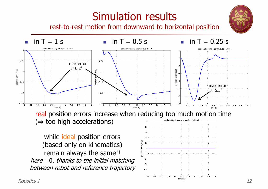
Simulation resultsrest-to-rest motion from downward to horizontal position

n in T = 1 s n in T = 0.5 s n in T = 0.25 s

real position errors increase when reducing too much motion time(⇒ too high accelerations)

max error≈ 0.2°

max error≈ 5.5°

Robotics 1 12

while ideal position errors(based only on kinematics)remain always the same!!

here ≡ 0, thanks to the initial matchingbetween robot and reference trajectory

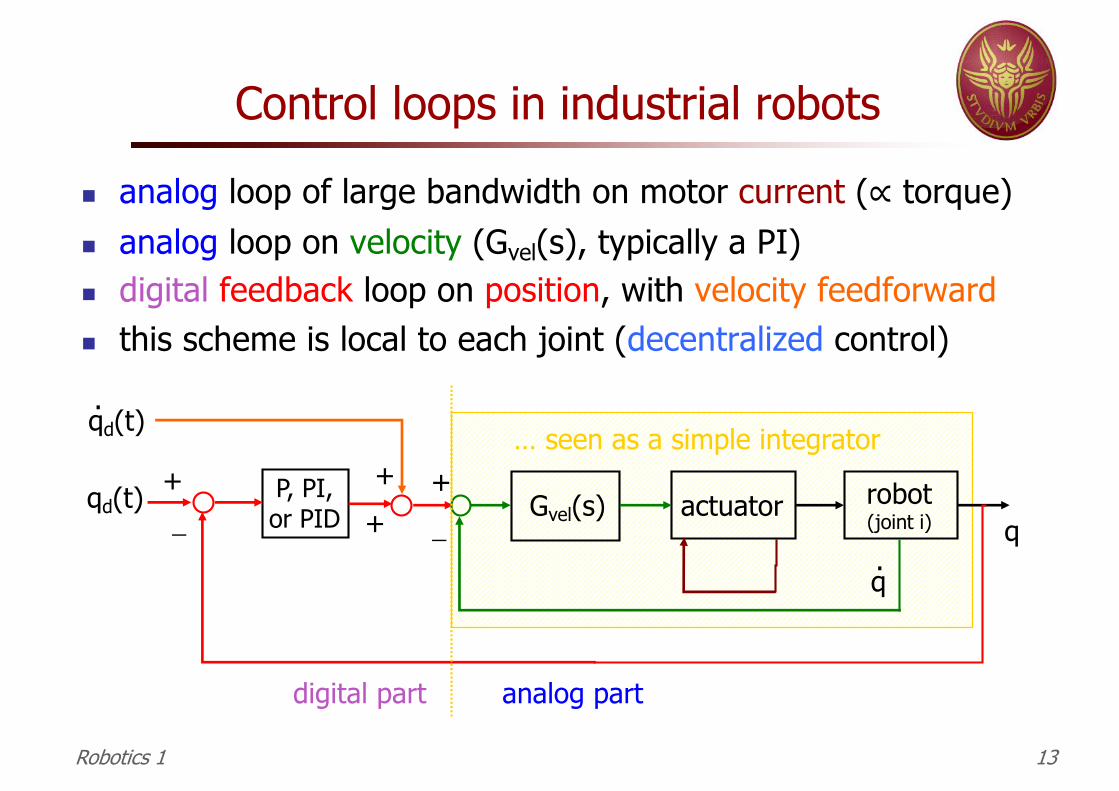
… seen as a simple integrator

Control loops in industrial robots

n analog loop of large bandwidth on motor current (∝ torque)n analog loop on velocity (Gvel(s), typically a PI)n digital feedback loop on position, with velocity feedforwardn this scheme is local to each joint (decentralized control)

robot(joint i)actuator

qP, PI,or PID

qd(t)

qd(t).

+ ++

+-

Gvel(s)

q.

-

digital part analog part

Robotics 1 13

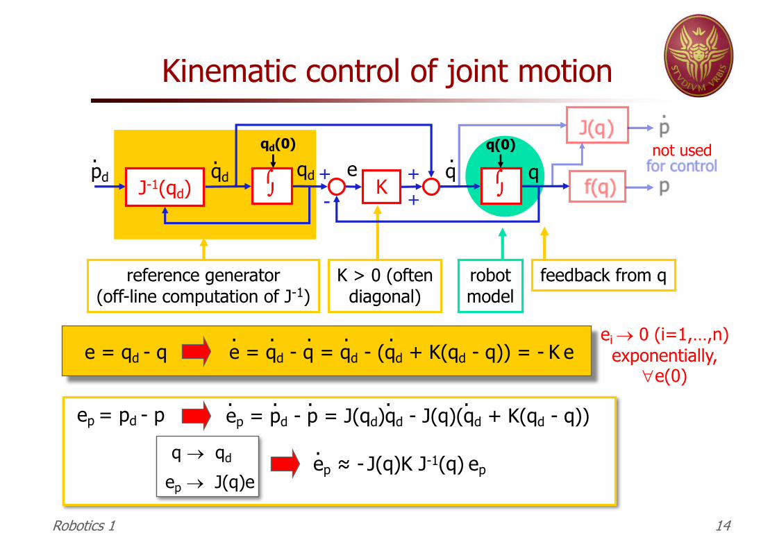
Kinematic control of joint motion

óõ K +-

+ +pd.

qd. qd

J-1(qd)óõ

q.

q

reference generator(off-line computation of J-1)

feedback from qK > 0 (oftendiagonal)

q(0)qd(0)

robotmodel

enot used

e = qd - q e = qd - q = qd - (qd + K(qd - q)) = - K eei ® 0 (i=1,…,n)

exponentially,"e(0)

. . . . .

ep = pd - p = J(qd)qd - J(q)(qd + K(qd - q))ep = pd - p

q ® qd

ep ® J(q)eep ≈ - J(q)K J-1(q) ep.

. . . ..

Robotics 1 14

robotmodel

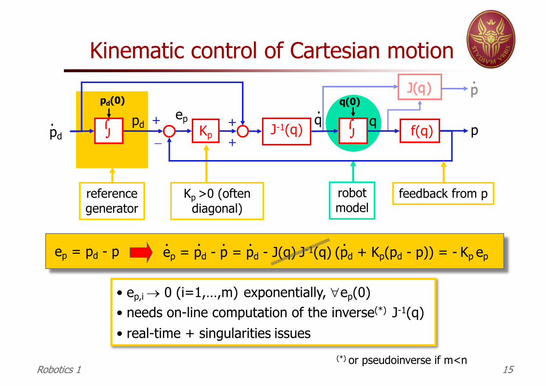
Kinematic control of Cartesian motion

óõ Kp +-

+ +pd. pd ó

õq.

q p

referencegenerator

feedback from pKp >0 (often diagonal)

pd(0)

J-1(q) f(q)

q(0)

• ep,i ® 0 (i=1,…,m) exponentially, "ep(0)• needs on-line computation of the inverse(*) J-1(q) • real-time + singularities issues

ep

Robotics 1 15

ep = pd - p ep = pd - p = pd - J(q) J-1(q) (pd + Kp(pd - p)) = - Kp ep. . . . .

(*) or pseudoinverse if m<n

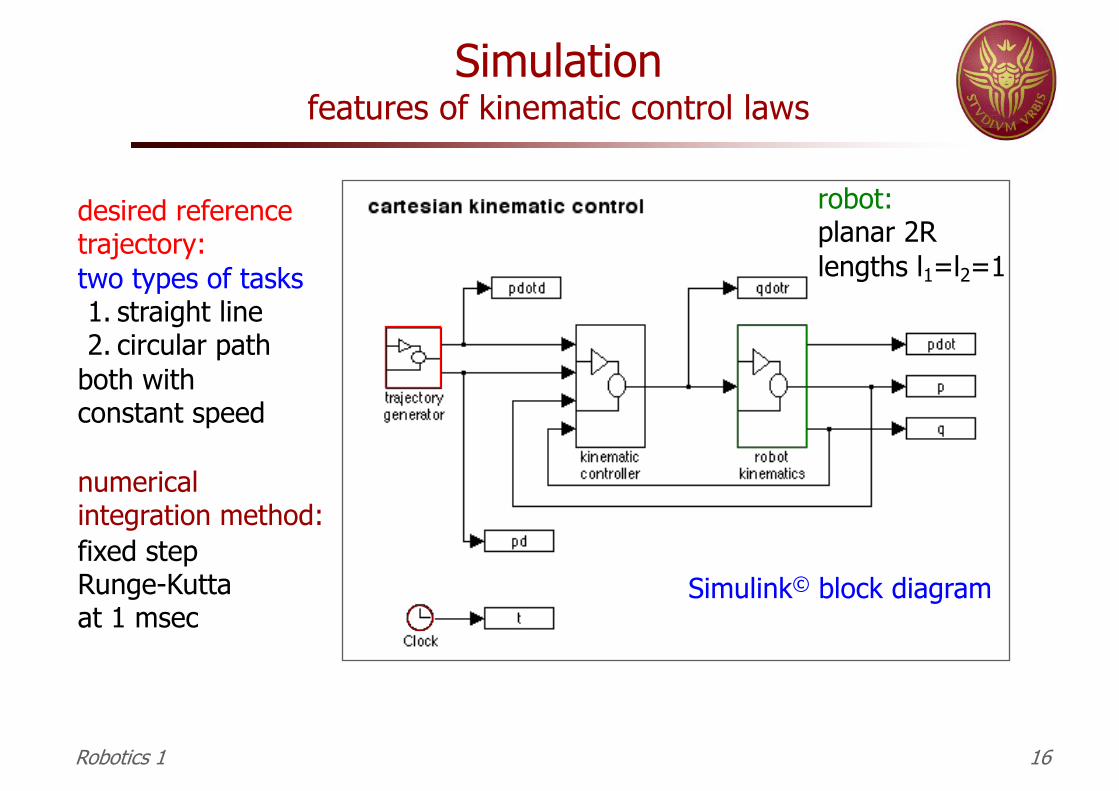
Simulationfeatures of kinematic control laws

Simulink© block diagram

desired referencetrajectory:two types of tasks1. straight line 2. circular path

both withconstant speed

robot:planar 2Rlengths l1=l2=1

numericalintegration method:fixed stepRunge-Kuttaat 1 msec

Robotics 1 16

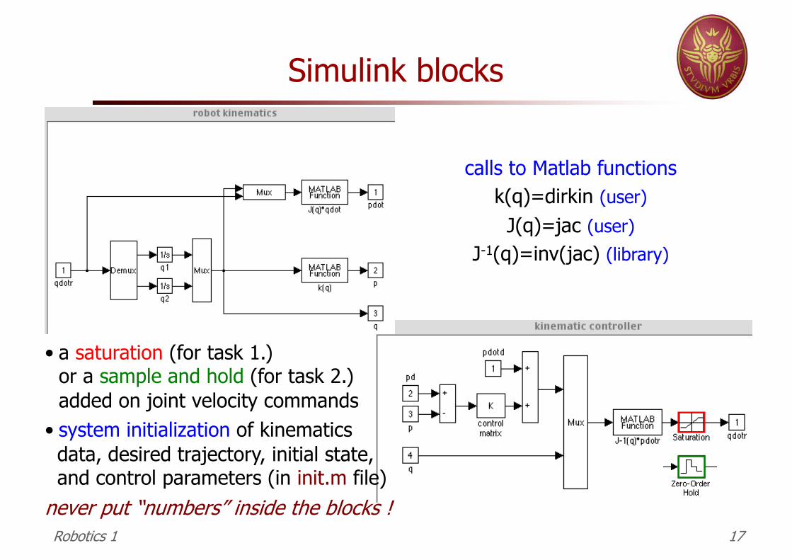
Simulink blocks

calls to Matlab functionsk(q)=dirkin (user)J(q)=jac (user)

J-1(q)=inv(jac) (library)

• a saturation (for task 1.)or a sample and hold (for task 2.)added on joint velocity commands

• system initialization of kinematicsdata, desired trajectory, initial state, and control parameters (in init.m file)

never put “numbers” inside the blocks !Robotics 1 17

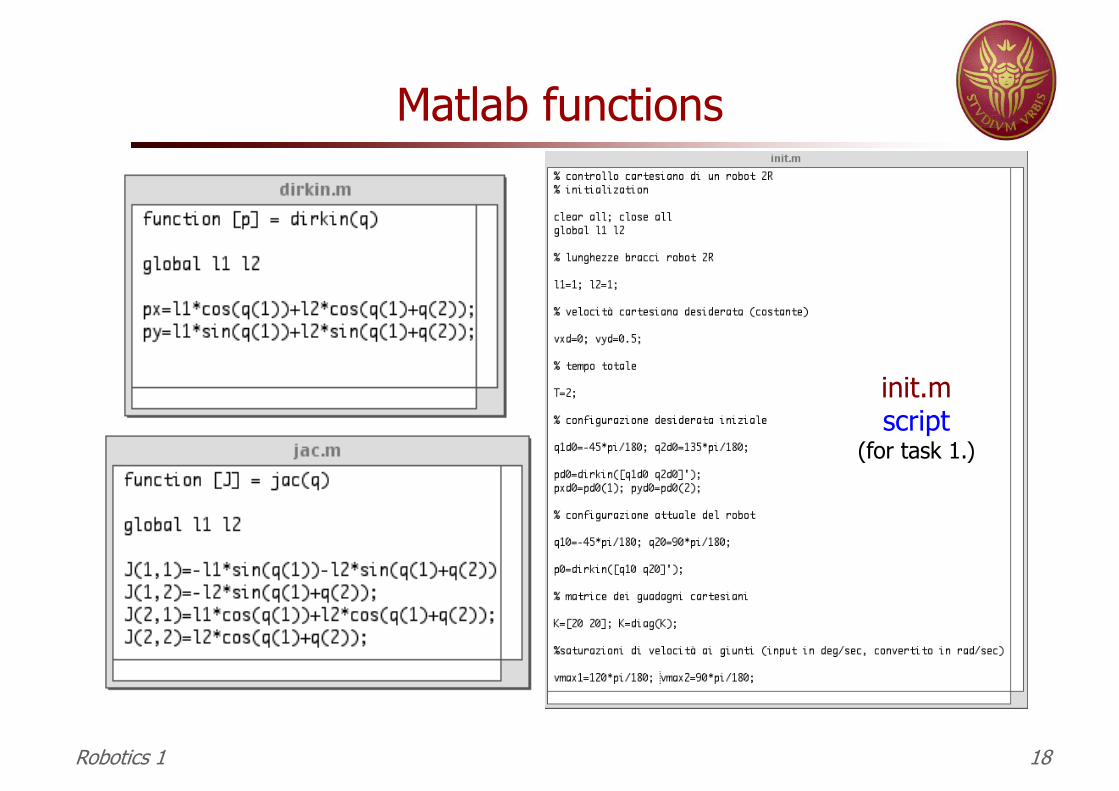
Matlab functions

init.mscript

(for task 1.)

Robotics 1 18

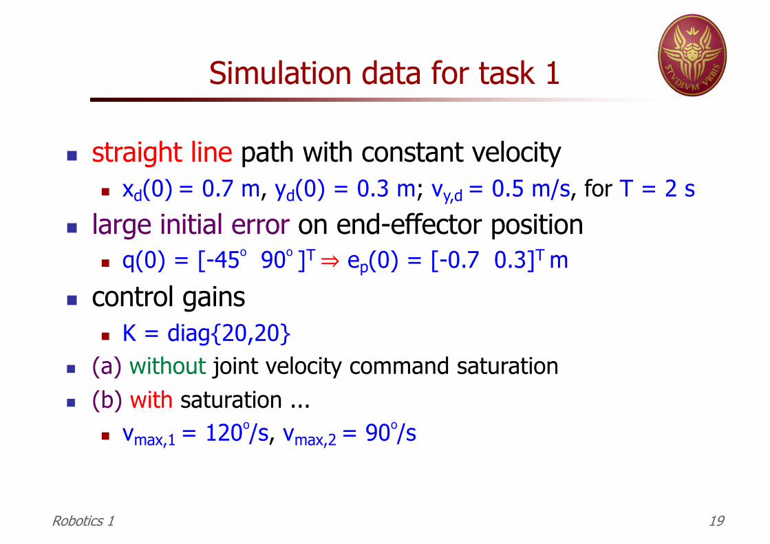
Simulation data for task 1

n straight line path with constant velocity n xd(0) = 0.7 m, yd(0) = 0.3 m; vy,d = 0.5 m/s, for T = 2 s

n large initial error on end-effector positionn q(0) = [-45o 90o ]T ⇒ ep(0) = [-0.7 0.3]T m

n control gainsn K = diag{20,20}

n (a) without joint velocity command saturationn (b) with saturation ...

n vmax,1 = 120o/s, vmax,2 = 90o/s

Robotics 1 19

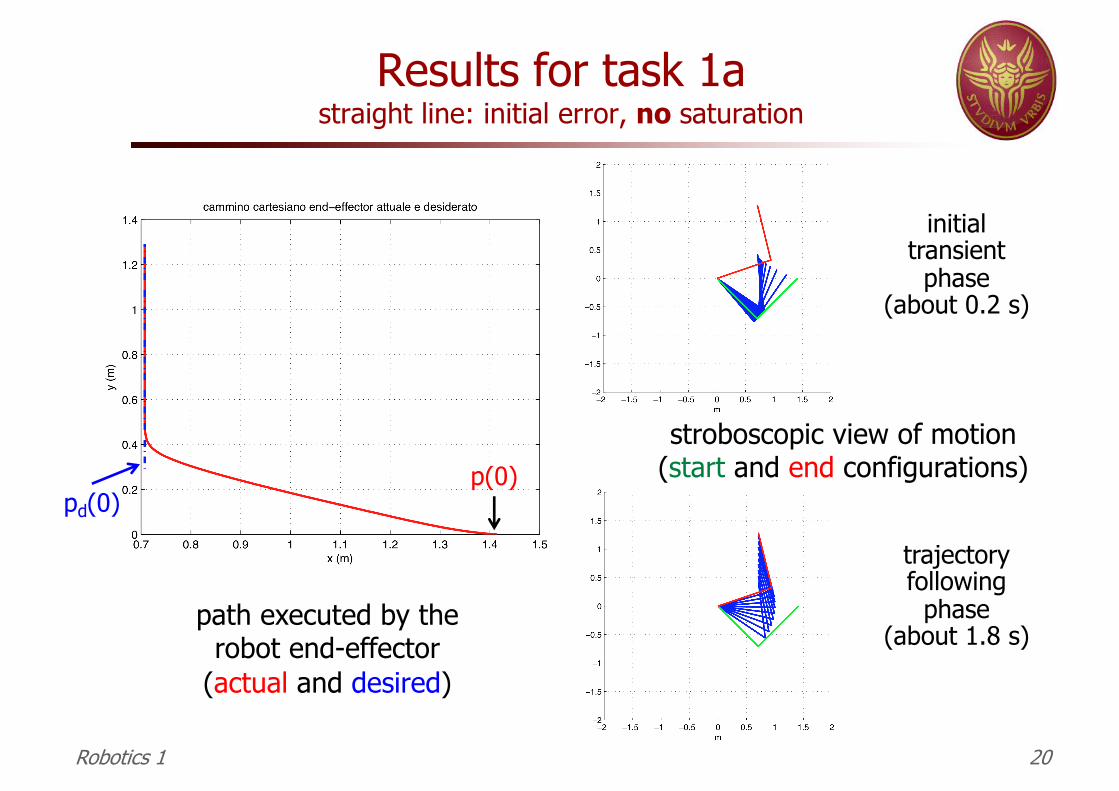
Results for task 1astraight line: initial error, no saturation

path executed by the robot end-effector

(actual and desired)

Robotics 1 20

stroboscopic view of motion(start and end configurations)

initialtransientphase

(about 0.2 s)

trajectoryfollowing

phase(about 1.8 s)

p(0)pd(0)

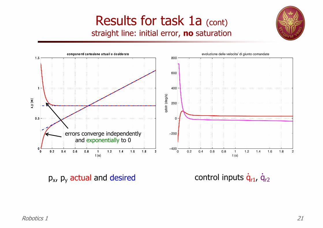
Results for task 1a (cont)straight line: initial error, no saturation

px, py actual and desired control inputs qr1, qr2. .

Robotics 1 21

errors converge independentlyand exponentially to 0

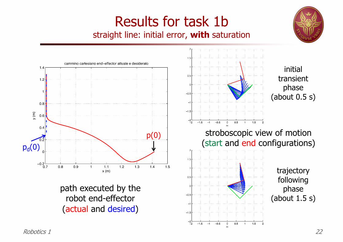
Results for task 1bstraight line: initial error, with saturation

path executed by the robot end-effector

(actual and desired)

Robotics 1 22

initialtransientphase

(about 0.5 s)

trajectoryfollowing

phase(about 1.5 s)

p(0)pd(0)

stroboscopic view of motion(start and end configurations)

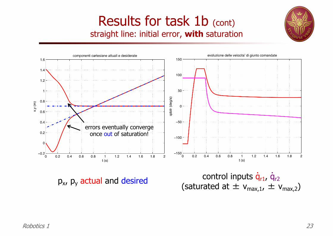
Results for task 1b (cont)straight line: initial error, with saturation

px, py actual and desired control inputs qr1, qr2(saturated at ± vmax,1, ± vmax,2)

. .

Robotics 1 23

errors eventually convergeonce out of saturation!

Simulation data for task 2

n circular path with constant velocity n centered at (1.014,0) with radius R = 0.4 m; n v = 2 m/s, performing two rounds ⇒ T ≈ 2.5 s

n zero initial error on Cartesian position (“match”)n q(0) = [-45o 90o ]T⇒ ep(0) = 0

n (a) ideal continuous case (1 kHz), even without feedbackn (b) with sample and hold (ZOH) of Thold = 0.02 s (joint

velocity command updated at 50 Hz), but without feedbackn (c) as before, but with Cartesian feedback using the gains

n K = diag{25,25}

Robotics 1 24

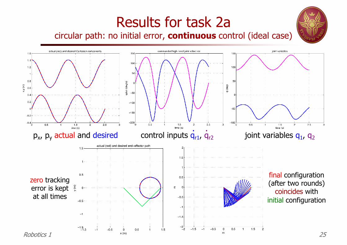
Results for task 2acircular path: no initial error, continuous control (ideal case)

px, py actual and desired control inputs qr1, qr2. .

Robotics 1 25

joint variables q1, q2

final configuration(after two rounds)

coincides withinitial configuration

zero trackingerror is keptat all times

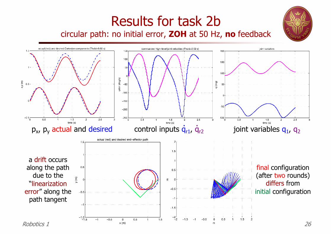
Results for task 2bcircular path: no initial error, ZOH at 50 Hz, no feedback

px, py actual and desired control inputs qr1, qr2. .

Robotics 1 26

joint variables q1, q2

a drift occursalong the path

due to the“linearization

error” along the path tangent

final configuration(after two rounds)

differs frominitial configuration

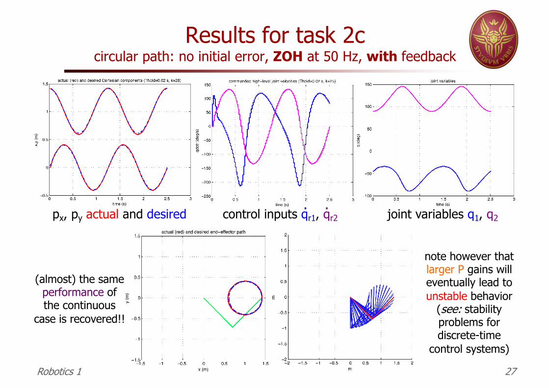
Results for task 2ccircular path: no initial error, ZOH at 50 Hz, with feedback

px, py actual and desired control inputs qr1, qr2. .

Robotics 1 27

joint variables q1, q2

(almost) the sameperformance ofthe continuous

case is recovered!!

note however thatlarger P gains willeventually lead to unstable behavior

(see: stability problems for discrete-time

control systems)

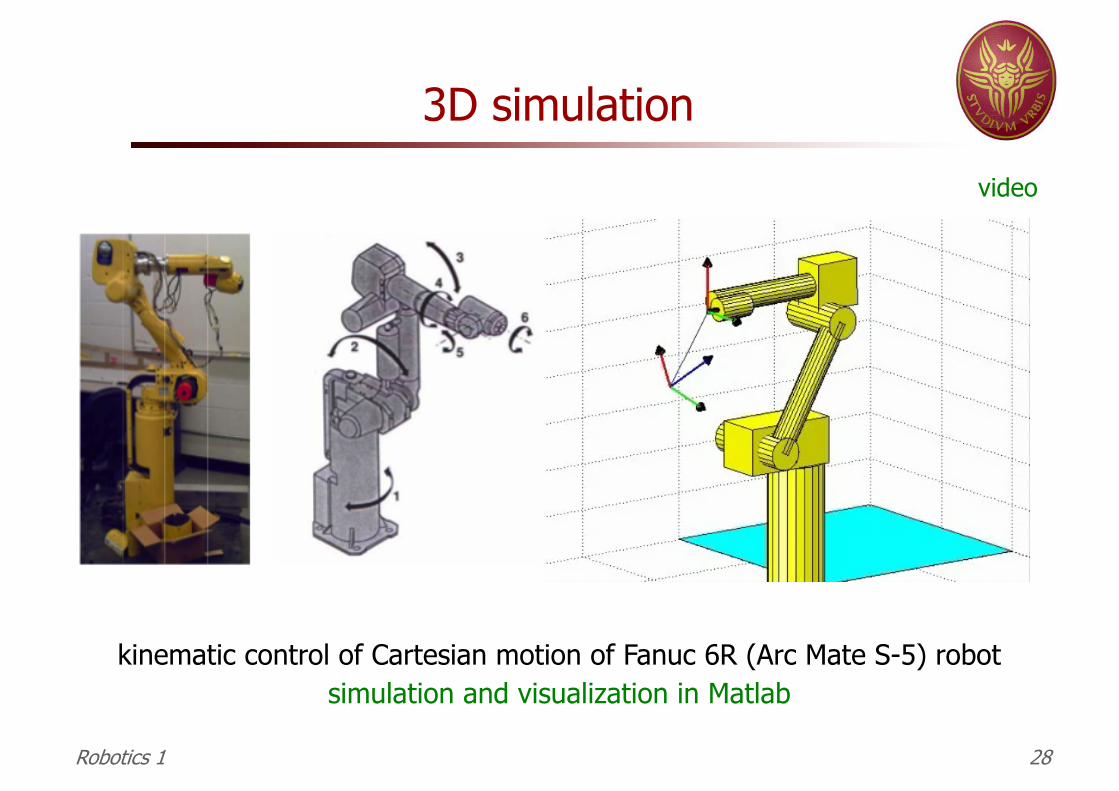
3D simulation

kinematic control of Cartesian motion of Fanuc 6R (Arc Mate S-5) robotsimulation and visualization in Matlab

video

Robotics 1 28

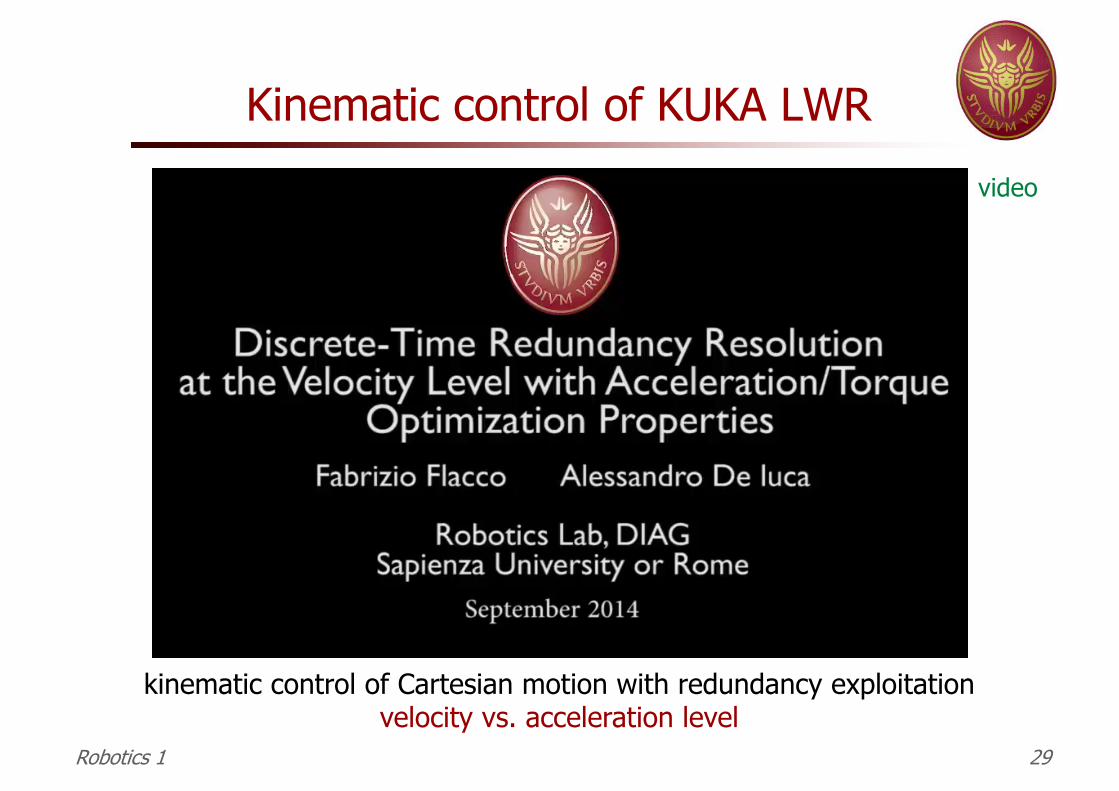
Kinematic control of KUKA LWR

kinematic control of Cartesian motion with redundancy exploitationvelocity vs. acceleration level

video

Robotics 1 29