Embed Size (px)
Citation preview

Robotics 2
Prof. Alessandro De Luca
Robot Interactionwith the Environment
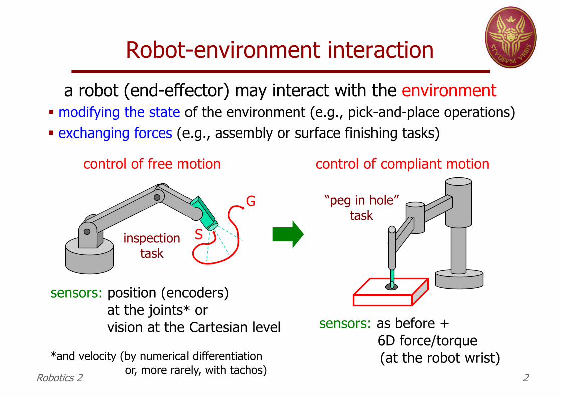
Robot-environment interactiona robot (end-effector) may interact with the environment
§ modifying the state of the environment (e.g., pick-and-place operations)§ exchanging forces (e.g., assembly or surface finishing tasks)
control of compliant motion
sensors: as before +6D force/torque (at the robot wrist)
“peg in hole”task
Robotics 2 2
sensors: position (encoders) at the joints* or vision at the Cartesian level
S
G
control of free motion
inspectiontask
*and velocity (by numerical differentiation or, more rarely, with tachos)

Robot compliance
PASSIVE robot end-effector equipped with mechatronic devices that “comply” with the generalized forces applied at the TCP = Tool Center Point
ACTIVErobot is moved by a control law so as to react in a desired way to generalized forces applied at the TCP (typically measured by a F/T sensor)
Robotics 2 3
RCC = Remote Center of Compliance device
§ admittance controlcontact forces ⇒ velocity commands
§ stiffness/compliance controlcontact displacements ⇒ force commands
§ impedance controlcontact displacements ⇔ contact forces

RCC device
flexible(elastic)elements
RCC models of different size
by ATI
Robotics 2 4

RCC behaviorin case of misalignment errors in assembly tasks
Robotics 2 5

Effects of RCC positioning
too high... too low...
Robotics 2 6
correct!(TCP = RCC)

Typical evolution of assembly forces
chamfer angle 𝛽 = to ease the insertion, related also to the tolerances of the hole
Robotics 2 7
“peg-in-hole” task

Active compliancefor contour following
Robotics 2 8

Active compliance“matching” of mechanical parts
Robotics 2 9

Tasks with environment interactionn mechanical machining
n deburring, surface finishing, polishing, assembly,...n tele-manipulation
n force feedback improves performance of human operators in master-slave systems
n contact exploration for shape identificationn force and velocity/vision sensor fusion allow 2D/3D geometric
identification of unknown objects and their contour followingn dexterous robot hands
n power grasp and fine in-hand manipulation require force/motion cooperation and coordinated control of the multiple fingers
n cooperation of multi-manipulator systemsn the environment includes one of more other robots with their own
dynamic behaviorsn physical human-robot interaction
n humans as active, dynamic environments that need to be handled under full safety premises …
Robotics 2 10

Examples of mechanical machining
Robotics 2 11
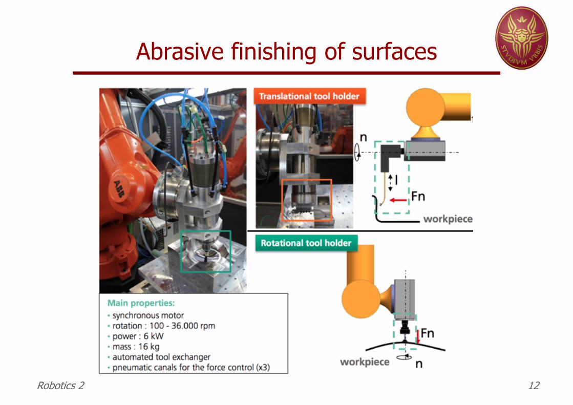
Abrasive finishing of surfaces
Robotics 2 12

Abrasive finishing of surfaces
Robotics 2 13
video
technological processes: cold forging of surfacesand hammer peening by pneumatic machine

Non-contact surface finishing
Robotics 2 14
Fluid Jet technology
Pulsed Laser technology
video
video
H2020 EU project for theFactory of the Future (FoF)

In all cases ...
n for physical interaction tasks, the desired motion specification and execution should be integrated with complementary data for the desired force
è hybrid planning and control objectivesn the exchanged forces/torques at the contact(s) with the
environment can be explicitly set under control or simply kept limited in an indirect way
Robotics 2 15

Evolution of control approachesa bit of history from the late 70’s-mid ‘80s …
n explicit control of forces/torques only [Whitney]n used in quasi-static operations (assembly) in order to avoid deadlocks
during part insertionn active admittance and compliance control [Paul, Shimano, Salisbury]
n contact forces handled through position (stiffness) or velocity (damping) control of the robot end-effector
n robot reacts as a compressed spring (with damper) in selected/all directionsn impedance control [Hogan]
n a desired dynamic behavior is imposed to the robot-environment interaction, e.g., a “model” with forces acting on a mass-spring-damper
n mimics the human arm behavior moving in an unknown environmentn hybrid force-motion control [Mason]
n decomposes the task space in complementary sets of directions where either force or motion is controlled, based onn a purely kinematic robot model [Raibert, Craig]n the actual dynamic model of the robot [Khatib]
appropriate for fast and accurate motion in dynamic interaction...Robotics 2 16

Interaction tasks of interest
interaction tasks with the environment that requiren accurate following/reproduction by the robot end-effector of desired
trajectories (even at high speed) defined on the surface of objectsn control of forces/torques applied at the contact with environments
having low (soft) or high (rigid) stiffness
robot
turninga crank
e.g., opening a door
deburring task
e.g., removing extra glue fromthe border of a car windshield
Robotics 2 17

Robotized deburring of windshields
c/o ABB Excellence Center in Cecchina (Roma), 2002
Robotics 2 18

Impedance vs. Hybrid control
n environment = mechanical system undergoing small but finite deformations
n contact forces arise as the result of a balance of two coupled dynamic systems (robot+environment)
è desired dynamic characteristics are assigned to the force/motion interaction
n a rigid environment reduces the degrees of freedom of the robot when in (bi-/uni-lateral) contact
n contact forces result from attempts to violate geometric constraints imposed by the environment
è task space is decomposed in sets of directions where only motion or only reaction forces are feasible
environment model ( domain of control application)impedance control hybrid force/motion control
§ the required level of knowledge about the environment geometry is only apparently different between the two control approaches
§ however, measuring contact forces may not be needed in impedance control, while it always necessary in hybrid force/motion control
Robotics 2 19

Impedance vs. Hybrid controln opening a door with a mobile
manipulator under impedance control
n piston insertion in a motor based on hybrid control of force-position (visual)
Robotics 2 20
video video

ù
A typical constrained situation …
robot
wrist6D F/T sensor
or RCC (or both)tool workpiece
(rigid)
the robot end-effector follows in a stable and accurateway the geometric profile of a very stiff workpiece,
while applying a desired contact force
Robotics 2 21

An unusual compliant situation …
Trevelyan (AUS): Oracle robotic system in a test dated 1981…is the sheep happy?
Robotics 2 22

A mixed interaction situation
processing/reasoning on force measurements leads to a sequence of fine motions
⇒ correct completion of insertion task withhelp of (sufficiently large) passive compliance
1. approach 2. search 3. insertion
X,Y-axescontrol
Z-axiscontrol
Robotics 2 23

Ideally constrained contact situation
𝑚𝑓&
𝑓'
𝑓(
𝑥( = 𝑐
𝑓( = −𝑓&
“ideal” = robot (sketched here as a Cartesian mass)+ environment are both infinitely STIFF(and without friction at the contact)
Robotics 2 24
a first possible modeling choice for very stiff environments
𝑥 < 𝑐 𝑓( = 0
𝑥 = 𝑐𝑓& ≥ 0
�̇� = 0�̈� = 0
𝑚�̈� = 𝑓& + 𝑓(𝑚�̈� = 𝑓'

In more complex situations
Robotics 2 25
n how can we describe more complex contact situations, where the end-effector of an articulated robot (not yet reduced to a Cartesian mass via feedback linearization control) is constrainedto move on an environment surface with nonlinear geometry?
n example: a planar 2R robot with end-effector moving on a circle
end-effectorconstrained on
a circular surface
(𝑥5, 𝑦5)𝑅
𝑥
𝑦
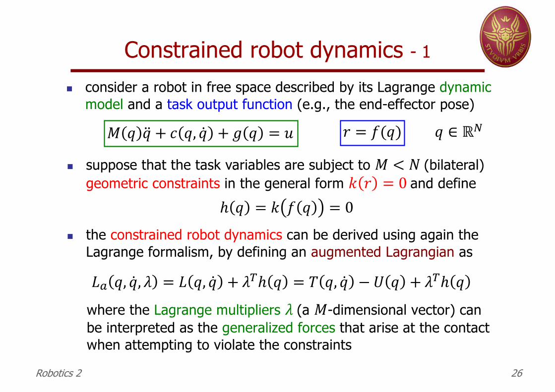
Constrained robot dynamics - 1
Robotics 2 26
n suppose that the task variables are subject to 𝑀 < 𝑁 (bilateral) geometric constraints in the general form 𝑘 𝑟 = 0 and define
ℎ 𝑞 = 𝑘 𝑓 𝑞 = 0
n the constrained robot dynamics can be derived using again the Lagrange formalism, by defining an augmented Lagrangian as
where the Lagrange multipliers 𝜆 (a 𝑀-dimensional vector) can be interpreted as the generalized forces that arise at the contact when attempting to violate the constraints
𝐿A 𝑞, �̇�, 𝜆 = 𝐿 𝑞, �̇� + 𝜆Bℎ 𝑞 = 𝑇 𝑞, �̇� − 𝑈 𝑞 + 𝜆Bℎ 𝑞
n consider a robot in free space described by its Lagrange dynamic model and a task output function (e.g., the end-effector pose)
𝑀 𝑞 �̈� + 𝑐 𝑞, �̇� + 𝑔 𝑞 = 𝑢 𝑟 = 𝑓(𝑞) 𝑞 ∈ ℝI

Constrained robot dynamics - 2
Robotics 2 27
contact forces doNOT produce work
n applying the Euler-Lagrange equations in the extended space of generalized coordinates 𝑞 AND multipliers 𝜆 yields
𝑑𝑑𝑡
𝜕𝐿A𝜕�̇�
B−
𝜕𝐿A𝜕𝑞
B=𝑑𝑑𝑡
𝜕𝐿𝜕�̇�
B−
𝜕𝐿𝜕𝑞
B−
𝜕𝜕𝑞 𝜆Bℎ(𝑞)
B
= 𝑢
𝜕𝐿A𝜕𝜆
B= ℎ 𝑞 = 0
𝐴 𝑞 =𝜕ℎ(𝑞)𝜕𝑞
where we defined the Jacobian of the constraints as the matrixsubject to
that will be assumed of full row rank (= 𝑀)
(★)𝑀 𝑞 �̈� + 𝑐 𝑞, �̇� + 𝑔 𝑞 = 𝑢 + 𝐴B(𝑞)𝜆
ℎ 𝑞 = 0

Constrained robot dynamics - 3
Robotics 2 28
n we can eliminate the appearance of the multipliers as followsn differentiate the constraints twice w.r.t. time
n substitute the joint accelerations from the dynamic model (★)(dropping dependencies)
n solve for the multipliers
to be replaced in the dynamic model...
the inertia-weighted pseudoinverse of the constraint Jacobian 𝐴
invertible 𝑀×𝑀 matrix,when 𝐴 is full rank constraint
forces 𝜆 areuniquely
determinedby the robotstate (𝑞, �̇�)
and input 𝑢 !!
ℎ 𝑞 = 0 ⇒ ℎ̇ =𝜕ℎ(𝑞)𝜕𝑞 �̇� = 𝐴 𝑞 �̇� = 0 ⇒ ℎ̈ = 𝐴 𝑞 �̈� + �̇� 𝑞 �̇� = 0
𝐴𝑀OP 𝑢 + 𝐴B𝜆 − 𝑐 − 𝑔 + �̇��̇� = 0
𝜆 = (𝐴𝑀OP𝐴B)OP 𝐴𝑀OP 𝑐 + 𝑔 − 𝑢 − �̇��̇�= 𝐴Q#
B 𝑐 + 𝑔 − 𝑢 − 𝐴𝑀OP𝐴B OP�̇��̇�

Constrained robot dynamics - 4
Robotics 2 29
n the final constrained dynamic model can be rewritten as
where 𝐴Q# 𝑞 = 𝑀OP(𝑞)𝐴B(𝑞)(𝐴(𝑞)𝑀OP(𝑞)𝐴B(𝑞))OP and with
n if the robot state (𝑞(0), �̇�(0)) at time 𝑡 = 0 satisfies the constraints, i.e.,
then the robot evolution described by the above dynamics will be consistent with the constraints for all 𝑡 ≥ 0 and for any 𝑢(𝑡)
§ this is a useful simulation model (constrained direct dynamics)
dynamically consistent projection matrix
ℎ 𝑞 0 = 0, 𝐴 𝑞 0 �̇�(0) = 0
𝜆 = 𝐴Q# (𝑞)B 𝑐(𝑞, �̇�) + 𝑔(𝑞) − 𝑢 − 𝐴 𝑞 𝑀OP 𝑞 𝐴B 𝑞 OP�̇�(𝑞)�̇�
𝑀 𝑞 �̈� = 𝐼 − 𝐴B(𝑞) 𝐴Q# (𝑞)B 𝑢 − 𝑐(𝑞, �̇� − 𝑔(𝑞)) −𝑀(𝑞)𝐴Q# (𝑞)�̇�(𝑞)�̇�

Robotics 2 30
Example – ideal massconstrained robot dynamics
𝑚𝑓&
𝑓'
𝑓(
𝑥 = 𝑐
𝑞 =𝑥𝑦
𝑢 =𝑓&𝑓' 𝑀 = 𝑚 0
0 𝑚
𝑀�̈� = 𝑢 robot dynamics in free motion
𝐼 − 𝐴B(𝑞) 𝐴Q# (𝑞)B = 0 0
0 1dynamically consistent
projection matrix
constrainedrobot dynamics𝑀 �̈�
�̈� = 𝑀�̈� = 0 00 1 𝑢 =
0𝑓'
𝜆 = − 𝐴Q# (𝑞)B𝑢 = − 1 0 𝑢 = −𝑓& multiplier (contact force 𝑓()
ℎ 𝑞 = 𝑥 − 𝑐 = 0 𝐴 𝑞 = 1 0 𝐴Q# 𝑞 = ⋯ = 10⇒ ⇒

Example – planar 2R robotconstrained robot dynamics
Robotics 2 31
𝑞1
𝑞2
𝑙1𝑙2
(𝑥5, 𝑦5)𝑅
𝑥
𝑦𝑘 𝑟 = 𝑥 − 𝑥5 X + 𝑦 − 𝑦5 X − 𝑅X = 0
𝑟 =𝑥𝑦
𝑟 = 𝑓 𝑞 = 𝑙P cos 𝑞P + 𝑙X cos 𝑞P + 𝑞X𝑙P sin 𝑞P + 𝑙X sin 𝑞P + 𝑞X
ℎ 𝑞 = 𝑘(𝑓 𝑞) =𝑙P cos 𝑞P + 𝑙X cos 𝑞P + 𝑞X − 𝑥5 X + 𝑙P sin 𝑞P + 𝑙X sin 𝑞P + 𝑞X − 𝑦5 X − 𝑅X = 0
ℎ̇ =𝜕𝑘𝜕𝑟
𝜕𝑟𝜕𝑞 �̇� =
2 𝑥 − 𝑥5 2 𝑦 − 𝑦5 𝐽_(𝑞)�̇�
= 2 𝑙P𝑐P + 𝑙X𝑐PX − 𝑥5 2 𝑙P𝑠P + 𝑙X𝑠PX − 𝑦5 𝐽_ 𝑞 �̇� = 𝐴(𝑞)�̇�

Reduced robot dynamics - 1
Robotics 2 32
n by imposing 𝑀 constraints ℎ(𝑞) = 0 on the 𝑁 generalized coordinates 𝑞, it is also possible to reduce the description of the constrained robot dynamics to a 𝑁 −𝑀 dimensional configuration space
n start from constraint matrix 𝐴(𝑞) and select a matrix 𝐷(𝑞) such that
n define the (𝑁 −𝑀)-dimensional vector of pseudo-velocities 𝑣 as the linear combination (at a given 𝑞) of the robot generalized velocities
n inverse relationships (from “pseudo” to “generalized” velocities and accelerations) are given by
properties of block products in inverse matrices have been used for eliminating the appearance of �̇� (often 𝐹 is only known numerically)
is a nonsingular𝑁×𝑁 matrix
𝐴(𝑞)𝐷(𝑞)
𝐴(𝑞)𝐷(𝑞)
OP= 𝐸(𝑞) 𝐹(𝑞)
𝑣 = 𝐷(𝑞)�̇� �̇� = 𝐷 𝑞 �̈� + �̇�(𝑞)�̇�
�̇� = 𝐹 𝑞 𝑣 �̈� = 𝐹 𝑞 �̇� − 𝐸 𝑞 �̇� 𝑞 + 𝐹(𝑞)�̇�(𝑞) 𝐹 𝑞 𝑣

Reduced robot dynamics – 2whiteboard …
Robotics 2 33
𝐴(𝑞)𝐷(𝑞)
OP= 𝐸(𝑞) 𝐹(𝑞) a number of properties from this definition…
two matrix inverse products𝐴(𝑞)𝐷(𝑞) 𝐸(𝑞) 𝐹(𝑞) = 𝐴 𝑞 𝐸(𝑞) 𝐴 𝑞 𝐹(𝑞)
𝐷 𝑞 𝐸(𝑞) 𝐷 𝑞 𝐹(𝑞) =𝐼Q×Q 00 𝐼(IOQ)×(IOQ)
𝐸(𝑞) 𝐹(𝑞) 𝐴(𝑞)𝐷(𝑞) = 𝐸 𝑞 𝐴 𝑞 + 𝐹 𝑞 𝐷 𝑞 = 𝐼I×I
from pseudo-velocity 𝑣 = 𝐷(𝑞)�̇�since 𝐹 is a right inverse of thefull row rank matrix 𝐷 (𝐷𝐹 = 𝐼)
�̇� = 𝐹 𝑞 𝑣= 𝐷B(𝑞) 𝐷(𝑞)𝐷B(𝑞) OP𝑣
(in fact𝐷�̇� = 𝐷𝐹𝑣
= 𝑣)
differentiating w.r.t. time �̇� = 𝐹 𝑞 𝑣
�̈� = 𝐹�̇� + �̇�𝑣 = 𝐹�̇� + (�̇�𝐷)�̇�
three useful identities!
differentiating w.r.t. time �̇�𝐴 + 𝐸�̇� + �̇�𝐷 + 𝐹�̇� = 0 ◁
= 𝐹(𝑞)�̇� − 𝐸 𝑞 �̇� 𝑞 + 𝐹 𝑞 �̇� 𝑞 𝐹(𝑞)𝑣
(◁)= 𝐹�̇� − �̇�𝐴 + 𝐸�̇� + 𝐹�̇� 𝐹𝑣
0𝐼
�̇�𝐷

Reduced robot dynamics - 3
Robotics 2 34
n consider again the dynamic model (★), dropping dependencies
n since 𝐴𝐸 = 𝐼, multiplying on the left by 𝐸B isolates the multipliers
n since 𝐴𝐹 = 0, multiplying on the left by 𝐹B eliminates the multipliers
n substituting in the latter the generalized accelerations and velocities with the pseudo-accelerations and pseudo-velocities leads finally to
which is the reduced (𝑁 −𝑀)-dimensional dynamic modeln similarly, the expression of the multipliers becomes
invertible 𝑁 −𝑀 × 𝑁 −𝑀
positive definite matrix
𝑀�̈� + 𝑐 + 𝑔 = 𝑢 + 𝐴B𝜆
𝐸B 𝑀�̈� + 𝑐 + 𝑔 − 𝑢 = 𝜆
𝐹B𝑀�̈� = 𝐹B 𝑢 − 𝑐 − 𝑔
𝐹B𝑀𝐹 �̇� = 𝐹B 𝑢 − 𝑐 − 𝑔 +𝑀 𝐸�̇� + 𝐹�̇� 𝐹𝑣
(§)𝜆 = 𝐸B 𝑀𝐹�̇� −𝑀 𝐸�̇� + 𝐹�̇� 𝐹𝑣 + 𝑐 + 𝑔 − 𝑢

Robotics 2 35
Example – ideal massreduced robot dynamics
𝑚𝑓&
𝑓'
𝑓(
𝑥 = 𝑐
𝑞 =𝑥𝑦
𝑢 =𝑓&𝑓'
𝑀 = 𝑚 00 𝑚
𝑀�̈� = 𝑢 robot dynamics in free motion
ℎ 𝑞 = 𝑥 − 𝑐 = 0 𝐴 = 1 0⇒ ⇒ 𝐴𝐷 = 1 0
0 1 = 𝐸 𝐹
reducedrobot dynamics𝐹B𝑀𝐹 �̇� = 0 1 𝑚 0
0 𝑚01 �̇� = 𝑚�̈� = 𝑓' = 𝐹B𝑢
multiplier(contact force 𝑓()
𝜆 = 𝐸B 𝑀𝐹�̇� − 𝑢
= 1 0 𝑚 00 𝑚
01 �̈� −
𝑓&𝑓'
= − 1 0𝑓&𝑓'
= −𝑓&
𝑣 = 𝐷�̇� = �̇� pseudo-velocity

Robotics 2 36
a feasible selection of matrix 𝐷(𝑞)
robotJacobian
out of robotsingularities
𝑞1
𝑞2
𝑙1𝑙2
(𝑥5, 𝑦5)𝑅
𝑥
𝑦𝑘 𝑟 = 𝑥 − 𝑥5 X + 𝑦 − 𝑦5 X − 𝑅X = 0
𝑟 =𝑥𝑦
𝑣 = (scalar) value of end-effector velocity reduced
along the tangentto the constraint
𝐴 𝑞 = 2 𝑥 − 𝑥5 2 𝑦 − 𝑦5 𝐽_ 𝑞= 2 𝑙P𝑐P + 𝑙X𝑐PX − 𝑥5 2 𝑙P𝑠P + 𝑙X𝑠PX − 𝑦5 𝐽_ 𝑞
𝐷(𝑞) = −12𝑦 − 𝑦5
12𝑥 − 𝑥5 𝐽_ 𝑞 det
𝐴(𝑞)𝐷(𝑞) = 𝑅X h det 𝐽_(𝑞) ≠ 0
𝐴(𝑞)𝐷(𝑞)
OP= 𝐸(𝑞) 𝐹(𝑞)
a scalar𝑣 = 𝐷(𝑞)�̇� �̇� = 𝐹 𝑞 𝑣 = 𝐽_OP(𝑞)
j−2(𝑦 − 𝑦5)𝑅X
j2(𝑥 − 𝑥5)𝑅X
𝑣
Example – planar 2R robotreduced robot dynamics

Control based on reduced robot dynamics
Robotics 2 37
n the reduced 𝑁 − 𝑀 dynamic expressions are more compact but also more complex and less used for simulation purposes than the 𝑁-dimensional constrained dynamics
n however, they are useful for control design (reduced inverse dynamics)n in fact, it is straightforward to verify that the feedback linearizing
control law
applied to the reduced robot dynamics and to the expression (§) of the multipliers leads to the closed-loop system
𝑢 = 𝑐 + 𝑔 −𝑀 𝐸�̇� + 𝐹�̇� 𝐹𝑣 +𝑀𝐹𝑢P − 𝐴B𝑢X
�̇� = 𝑢P 𝜆 = 𝑢X
Note: these are exactly in the form of the ideal mass example of slide #24, with 𝑣 = �̇�, 𝑢P = 𝑓'/𝑚, λ = 𝑓(, 𝑢X = −𝑓& (being 𝑁 = 2, 𝑀 = 1, 𝑁 − 𝑀 = 1)

Compliant contact situation
𝐾(
Robotics 2 38
a second possible modeling choice for softer environments
𝑥 < 𝑐 𝑓( = 0𝑥 ≥ 𝑐 𝑓( = 𝐾((𝑥 − 𝑐)
𝑚�̈� = 𝑓& + 𝑓(𝑚�̈� = 𝑓'
𝑚𝑓&
𝑓'
𝑓(
𝑥( = 𝑐
compliance/impedancecontrol (in all directions) is here a good choicethat allows to handle§ uncertain position§ uncertain orientationof the wall
with 𝐾( > 0 being the stiffness of the environment

Robot-environment contact types modeled by a single elastic constant
𝐾 = 𝐾o
rigid environmentcompliantforce sensor
compliant environment
rigid robot(including
force sensor) 𝐾 = 𝐾(
𝐾o
𝐾(
negligible intermediatemass
Robotics 2 39
series of springs =sum of compliances
(inverse of stiffnesses)
1𝐾 =
1𝐾o+1𝐾(
𝐾 =𝐾o𝐾(𝐾o +𝐾(
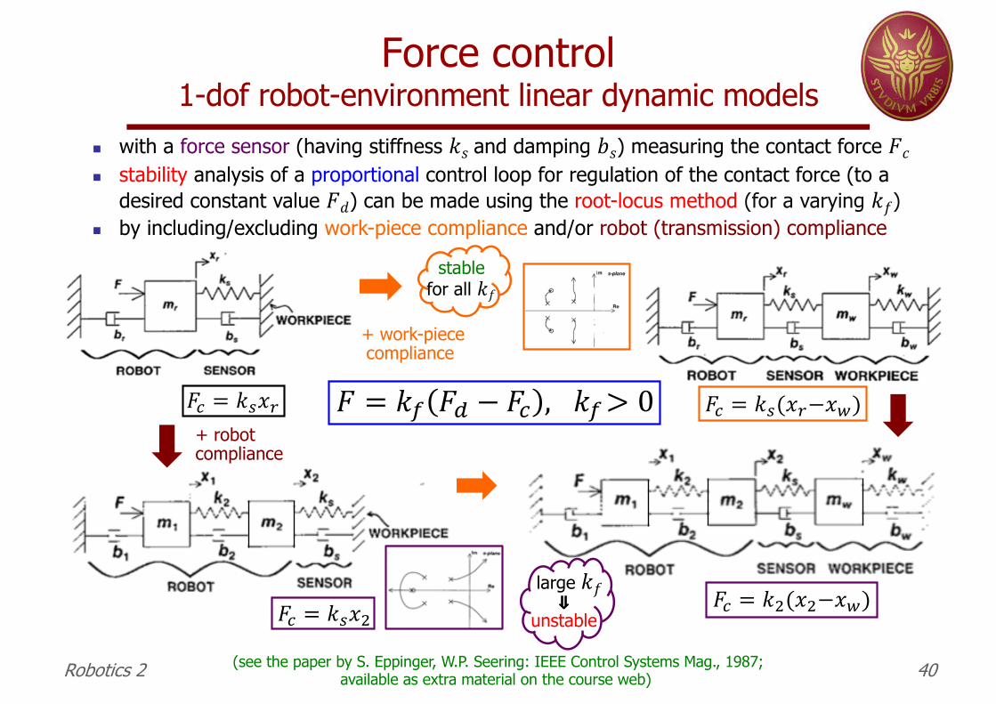
Force control 1-dof robot-environment linear dynamic models
Robotics 2 40
n with a force sensor (having stiffness 𝑘𝑠 and damping 𝑏𝑠) measuring the contact force 𝐹𝑐n stability analysis of a proportional control loop for regulation of the contact force (to a
desired constant value 𝐹𝑑) can be made using the root-locus method (for a varying 𝑘𝑓)n by including/excluding work-piece compliance and/or robot (transmission) compliance
(see the paper by S. Eppinger, W.P. Seering: IEEE Control Systems Mag., 1987;available as extra material on the course web)
+ work-piececompliance
+ robot compliance
large 𝑘𝑓⇓
unstable
stablefor all 𝑘𝑓
𝐹r = 𝑘o𝑥_ 𝐹r = 𝑘o(𝑥_−𝑥s)
𝐹r = 𝑘X(𝑥X−𝑥s)𝐹r = 𝑘o𝑥X
𝐹 = 𝑘t 𝐹u − 𝐹r , 𝑘t> 0

Tasks requiring hybrid control
the robot should turn a crankhaving a free-spinning handle
Robotics 2 41
two generalized directions of instantaneousfree motion
at the contact:tangential velocity& angular velocityaround handle axis
↕four directions of generalized reaction forcesat the contact

Tasks requiring hybrid control
Robotics 2 42
the robot should turn a crankhaving a fixed handle
one direction onlyof instantaneous
free motionat the contact:
tangential velocity
↕five directions of generalized reaction forcesat the contact

Tasks requiring hybrid control
the robot should push a mass elastically coupled to a wall and constrained in a guide
Robotics 2 43

Tasks requiring hybrid control
generalized hybrid modeling and control for dynamic environmentsA. De Luca, C. Manes: IEEE Trans. Robotics and Automation, vol. 10, no. 4, 1994
Robotics 2 44
direction of free motion control(no contact forces can be imposed)
direction of contact force control (no motion can be imposed)
dynamic direction of control:either motion is controlled
(and a contact force results)or contact force is controlled
(and a motion results)
KE
three sets of possible directions in the task frame