Robotics 2

Prof. Alessandro De Luca

Trajectory Tracking Control

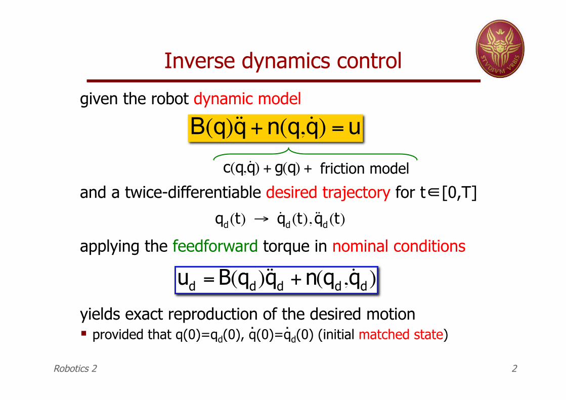
Inverse dynamics control

given the robot dynamic model

!

B(q)˙ ̇ q + n(q, ˙ q ) = u

and a twice-differentiable desired trajectory for t∈[0,T]

!

qd(t) " ˙ q d(t), ˙ ̇ q d(t)

applying the feedforward torque in nominal conditions

!

ud = B(qd)˙ ̇ q d + n(qd, ˙ q d)yields exact reproduction of the desired motion !  provided that q(0)=qd(0), q(0)=qd(0) (initial matched state)

!

c(q, ˙ q ) + g(q) + friction model

Robotics 2 2

. .

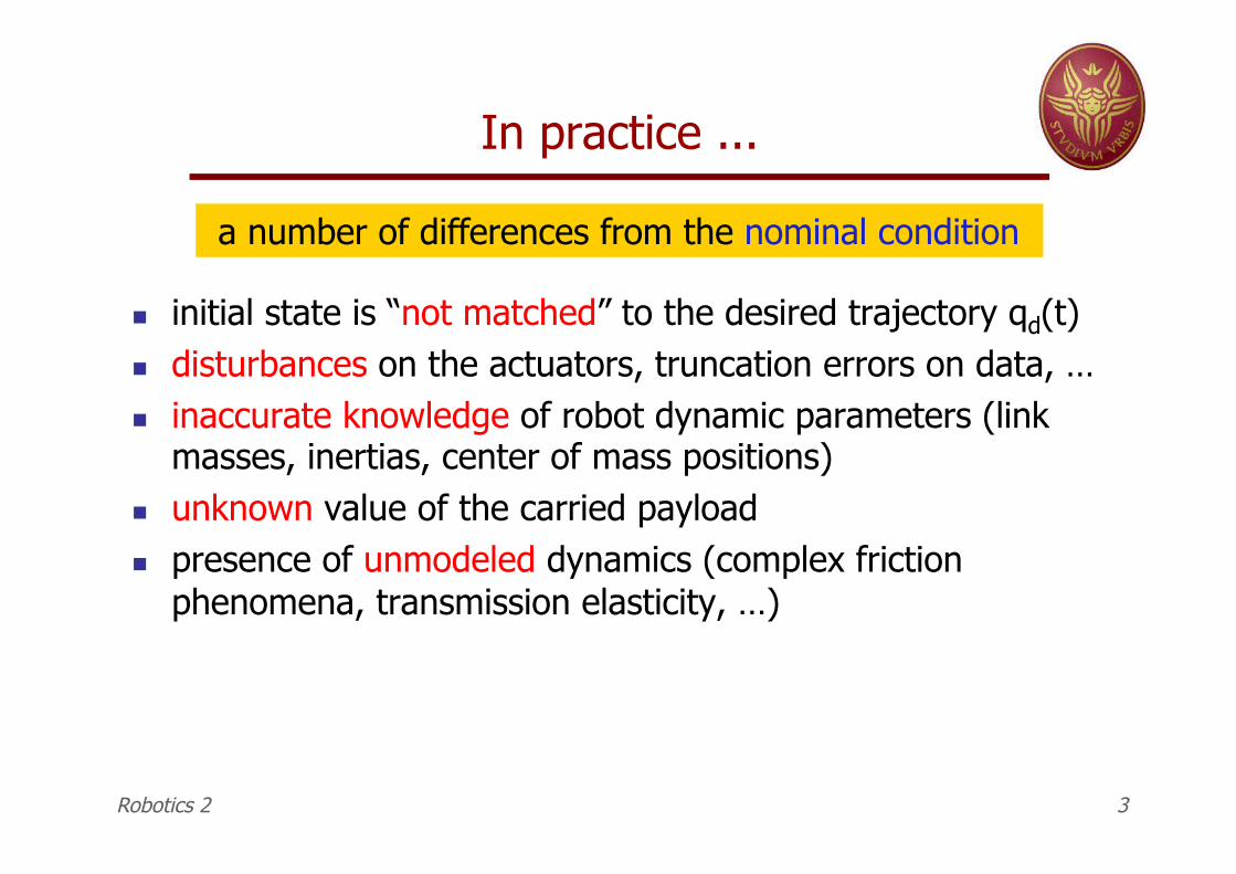
In practice ...

"  initial state is “not matched” to the desired trajectory qd(t) "  disturbances on the actuators, truncation errors on data, … "  inaccurate knowledge of robot dynamic parameters (link

masses, inertias, center of mass positions) "  unknown value of the carried payload "  presence of unmodeled dynamics (complex friction

phenomena, transmission elasticity, …)

a number of differences from the nominal condition

Robotics 2 3

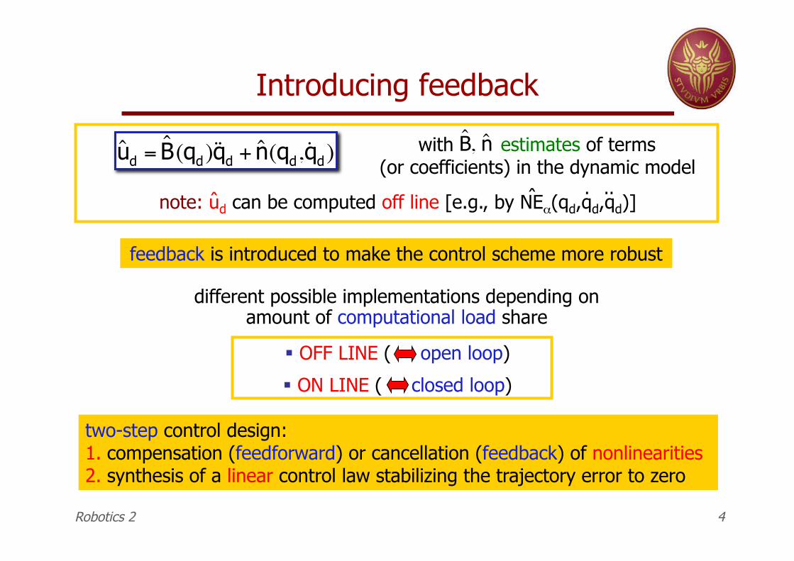
different possible implementations depending on amount of computational load share

!  OFF LINE ( open loop)

!  ON LINE ( closed loop)

Introducing feedback

!

ˆ u d = ˆ B (qd)˙ ̇ q d + ˆ n (qd, ˙ q d) with estimates of terms (or coefficients) in the dynamic model

note: ud can be computed off line [e.g., by NE!(qd,qd,qd)]

feedback is introduced to make the control scheme more robust

two-step control design: 1.  compensation (feedforward) or cancellation (feedback) of nonlinearities 2.  synthesis of a linear control law stabilizing the trajectory error to zero

Robotics 2 4

. ..

!

ˆ B , ˆ n

ˆ ˆ

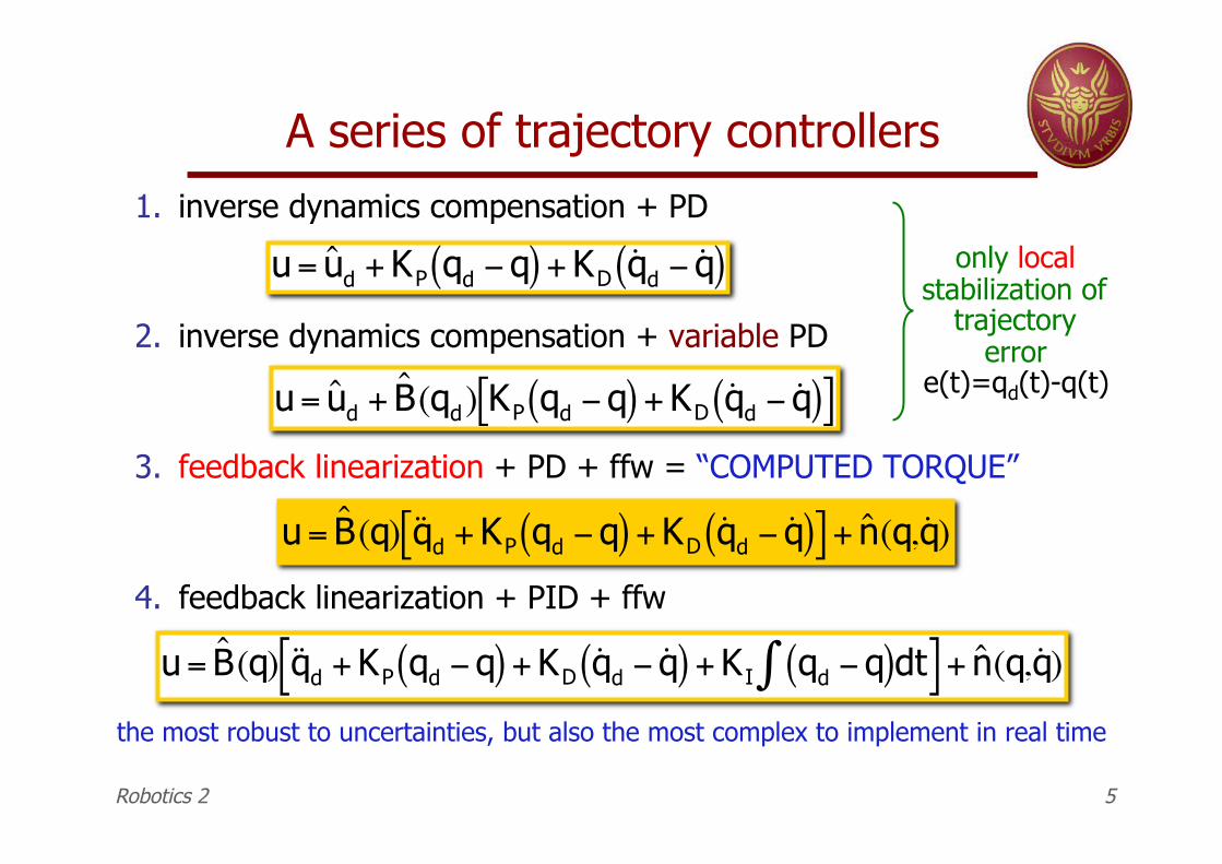
A series of trajectory controllers

1.  inverse dynamics compensation + PD

2.  inverse dynamics compensation + variable PD

3.  feedback linearization + PD + ffw = “COMPUTED TORQUE”

4.  feedback linearization + PID + ffw

!

u = ˆ u d + KP qd "q( ) + KD˙ q d " ˙ q ( )

!

u = ˆ u d + ˆ B (qd) KP qd "q( ) + KD˙ q d " ˙ q ( )[ ]

!

u = ˆ B (q) ˙ ̇ q d + KP qd "q( ) + KD˙ q d " ˙ q ( )[ ] + ˆ n (q, ˙ q )

!

u = ˆ B (q) ˙ ̇ q d + KP qd "q( ) + KD˙ q d " ˙ q ( ) + KI qd "q( )dt#[ ] + ˆ n (q, ˙ q )

the most robust to uncertainties, but also the most complex to implement in real time

only local stabilization of

trajectory error

e(t)=qd(t)-q(t)

Robotics 2 5

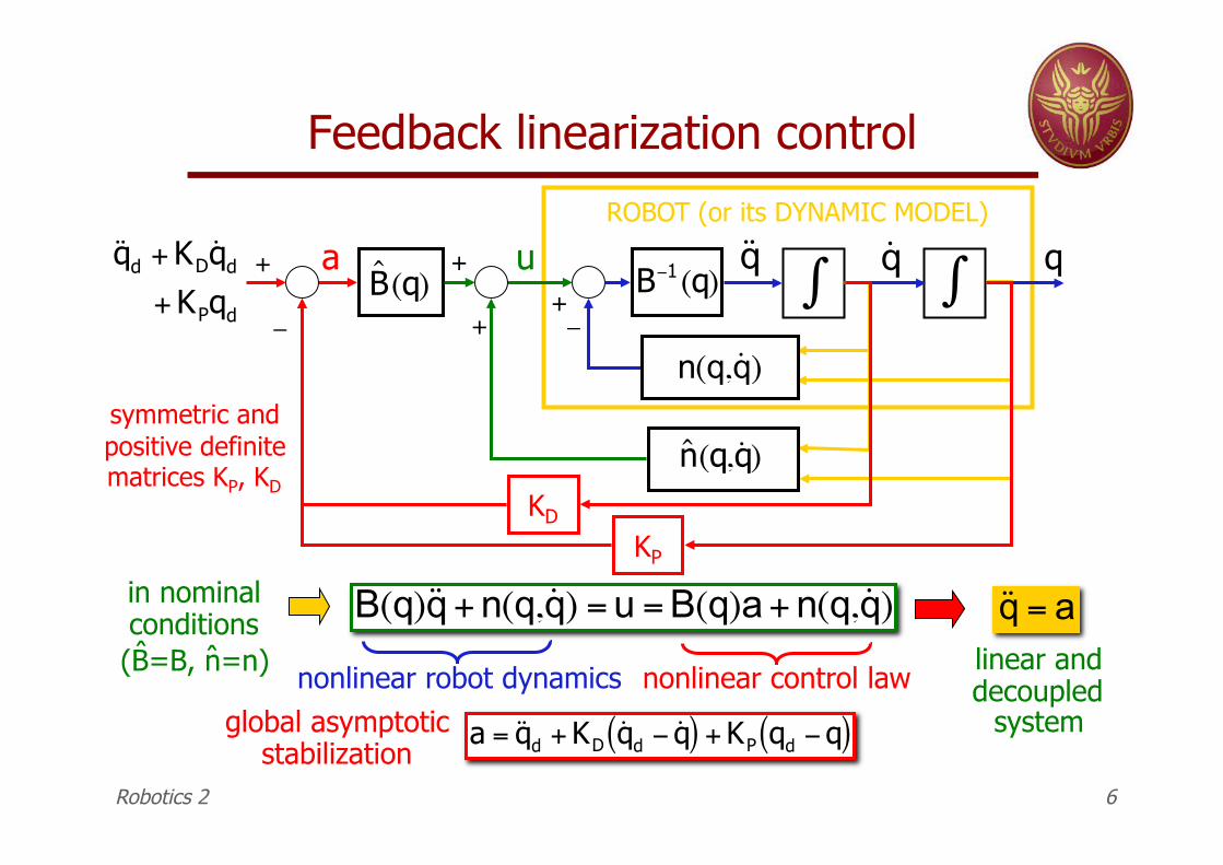
Feedback linearization control

+

!

"_

!

˙ q

!

˙ ̇ q

!

n(q, ˙ q )

+

!

ˆ n (q, ˙ q )

+

u

KD

KP

+

ROBOT (or its DYNAMIC MODEL)

in nominal conditions (B=B, n=n)

!

B(q)˙ ̇ q + n(q, ˙ q ) = u = B(q)a + n(q, ˙ q )

nonlinear robot dynamics nonlinear control law

!

˙ ̇ q = a

!

a = ˙ ̇ q d + KD˙ q d " ˙ q ( ) + KP qd "q( )

a

!

" q

!

˙ ̇ q d + KD˙ q d

+ KPqd

!

ˆ B (q)

!

B"1(q)_

linear and decoupled

system global asymptotic stabilization

symmetric and positive definite matrices KP, KD

Robotics 2 6

ˆ ˆ

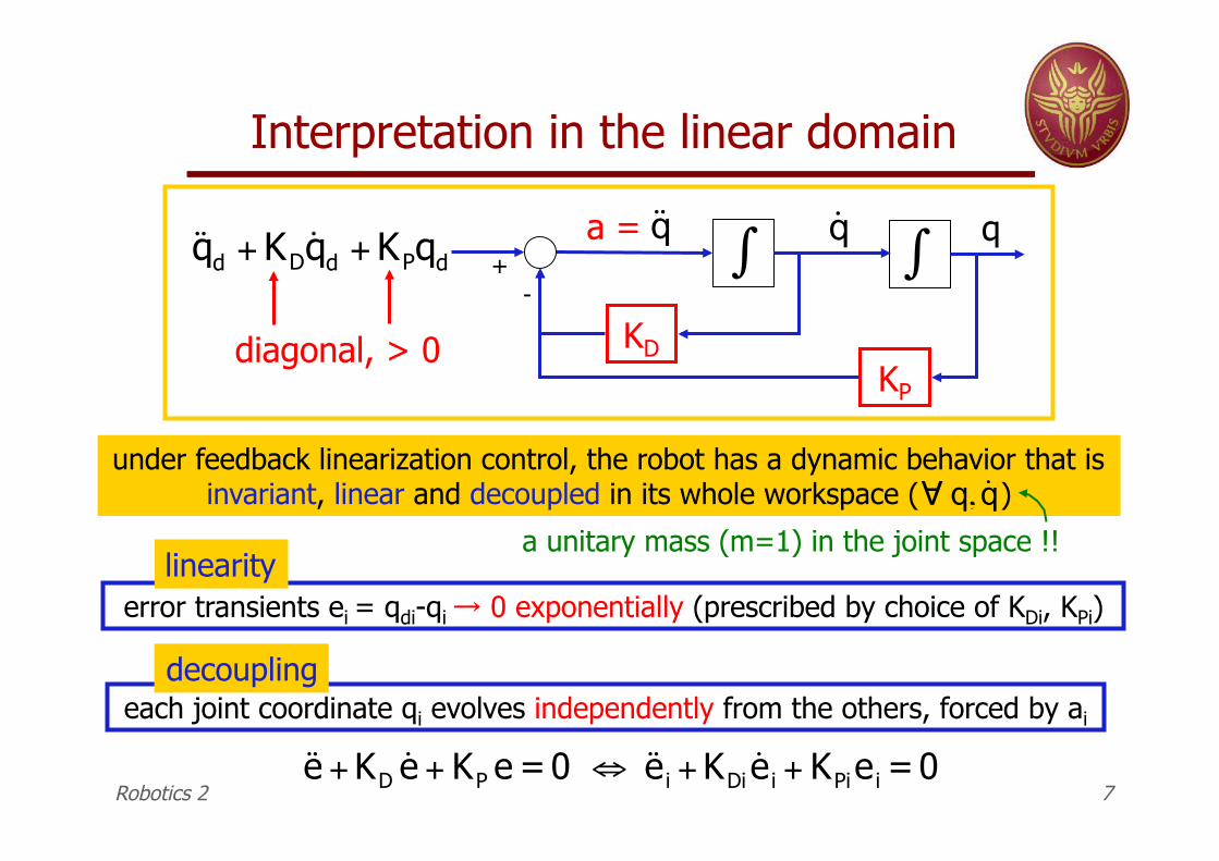
Interpretation in the linear domain

!

"

!

˙ q

!

˙ ̇ q

!

˙ ̇ q d + KD˙ q d + KPqd

KD

KP

- +

under feedback linearization control, the robot has a dynamic behavior that is invariant, linear and decoupled in its whole workspace ( )

diagonal, > 0

!

" q, ˙ q

each joint coordinate qi evolves independently from the others, forced by ai

a =

!

" q

error transients ei = qdi-qi → 0 exponentially (prescribed by choice of KDi, KPi)

linearity

decoupling

a unitary mass (m=1) in the joint space !!

Robotics 2 7

!

˙ ̇ e + KD˙ e + KP e =0 " ˙ ̇ e i + KDi

˙ e i + KPiei =0

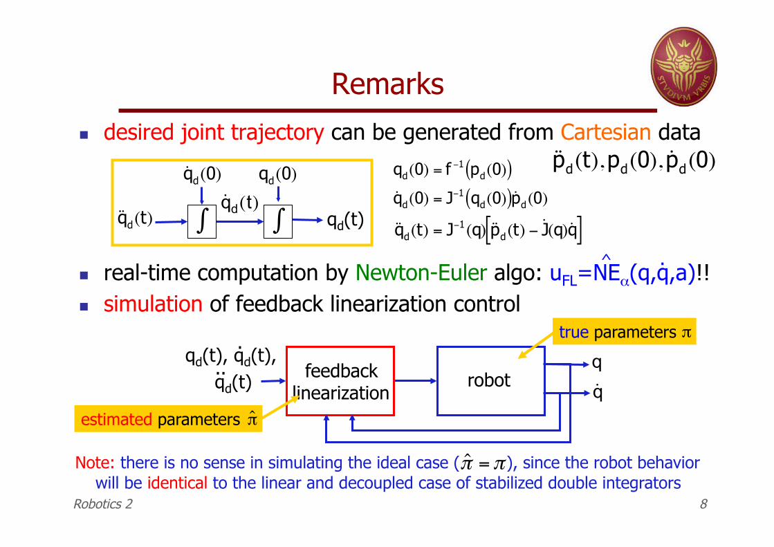
"  desired joint trajectory can be generated from Cartesian data

"  real-time computation by Newton-Euler algo: uFL=NE!(q,q,a)!! "  simulation of feedback linearization control

Remarks

!

˙ ̇ p d(t),pd(0), ˙ p d(0)

!

˙ ̇ q d(t) = J"1(q) ˙ ̇ p d(t) " ˙ J (q)˙ q [ ]

!

qd(0) = f "1 pd(0)( )˙ q d(0) = J"1 qd(0)( )˙ p d(0)

!

" qd(t)

!

˙ q d(0)

!

˙ q d(t)

feedback linearization

robot qd(t)

!

˙ q

!

q

estimated parameters

!

ˆ "

true parameters

!

"

!

"

Note: there is no sense in simulating the ideal case ( ), since the robot behavior will be identical to the linear and decoupled case of stabilized double integrators

!

ˆ " ="

qd(t), qd(t), .

..

!

qd(0)

!

˙ ̇ q d(t)

Robotics 2 8

. ^

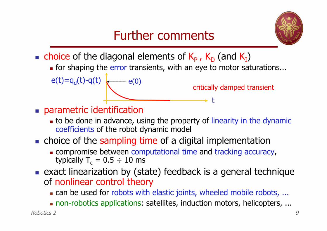
Further comments

"  choice of the diagonal elements of KP , KD (and KI) "  for shaping the error transients, with an eye to motor saturations...

"  parametric identification "  to be done in advance, using the property of linearity in the dynamic

coefficients of the robot dynamic model

"  choice of the sampling time of a digital implementation "  compromise between computational time and tracking accuracy,

typically Tc = 0.5 ÷ 10 ms

"  exact linearization by (state) feedback is a general technique of nonlinear control theory

"  can be used for robots with elastic joints, wheeled mobile robots, ... "  non-robotics applications: satellites, induction motors, helicopters, ...

critically damped transient e(t)=qd(t)-q(t)

t

e(0)

Robotics 2 9

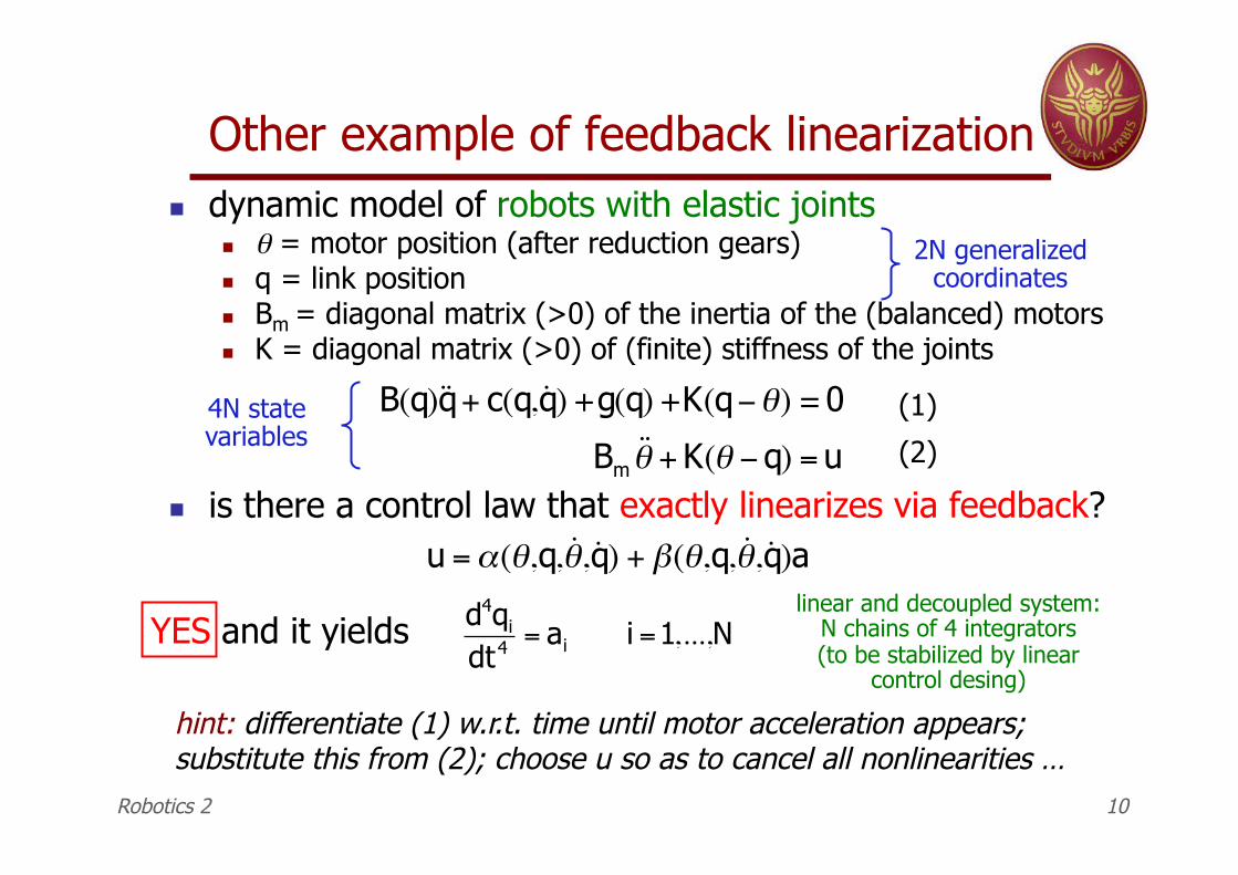
Other example of feedback linearization "  dynamic model of robots with elastic joints

"  ! = motor position (after reduction gears) "  q = link position "  Bm = diagonal matrix (>0) of the inertia of the (balanced) motors "  K = diagonal matrix (>0) of (finite) stiffness of the joints

"  is there a control law that exactly linearizes via feedback?

2N generalized coordinates

!

u ="(#,q, ˙ # , ˙ q ) + $(#,q, ˙ # , ˙ q )a

!

B(q)˙ ̇ q + c(q, ˙ q ) +g(q) +K(q"#) = 0

Bm˙ ̇ # + K(# "q) = u

(1)

(2)

4N state variables

hint: differentiate (1) w.r.t. time until motor acceleration appears; substitute this from (2); choose u so as to cancel all nonlinearities …

YES and it yields

!

d4qi

dt4 = ai i =1,...,Nlinear and decoupled system:

N chains of 4 integrators (to be stabilized by linear

control desing)

Robotics 2 10

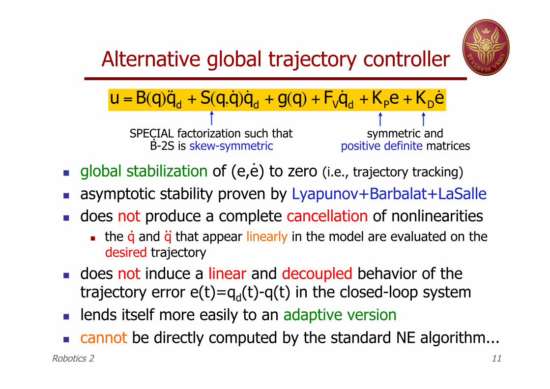
Alternative global trajectory controller

"  global stabilization of (e,e) to zero (i.e., trajectory tracking) "  asymptotic stability proven by Lyapunov+Barbalat+LaSalle "  does not produce a complete cancellation of nonlinearities

"  the q and q that appear linearly in the model are evaluated on the desired trajectory

"  does not induce a linear and decoupled behavior of the trajectory error e(t)=qd(t)-q(t) in the closed-loop system

"  lends itself more easily to an adaptive version "  cannot be directly computed by the standard NE algorithm...

!

u = B(q)˙ ̇ q d + S(q, ˙ q )˙ q d + g(q) + FV˙ q d + KPe + KD

˙ e

symmetric and positive definite matrices

SPECIAL factorization such that B-2S is skew-symmetric .

.

Robotics 2 11

. ..

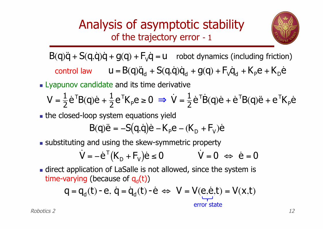
Analysis of asymptotic stability of the trajectory error - 1

"  Lyapunov candidate and its time derivative

!

B(q)˙ ̇ q + S(q, ˙ q )˙ q + g(q) + FV˙ q = u

!

u = B(q)˙ ̇ q d + S(q, ˙ q )˙ q d + g(q) + FV˙ q d + KPe + KD

˙ e robot dynamics (including friction)

control law

!

V = 12

˙ e TB(q) ˙ e + 12 eTKPe " 0

!

˙ V = 12

˙ e T ˙ B (q) ˙ e + ˙ e TB(q)˙ ̇ e + eTKP˙ e

"  the closed-loop system equations yield

!

B(q)˙ ̇ e = "S q, ˙ q ( ) ˙ e "KPe " (KD + FV)˙ e "  substituting and using the skew-symmetric property

!

˙ V = " ˙ e T KD + FV( ) ˙ e # 0"  direct application of LaSalle is not allowed, since the system is

time-varying (because of qd(t))

!

˙ V = 0 " ˙ e = 0

!

q = qd(t) - e, ˙ q = ˙ q d(t) - ˙ e " V = V(e, ˙ e ,t) = V(x,t)

Robotics 2 12

⇒

error state

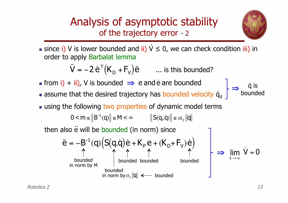
Analysis of asymptotic stability of the trajectory error - 2

"  since i) V is lower bounded and ii) V ! 0, we can check condition iii) in order to apply Barbalat lemma

... is this bounded?

"  from i) + ii), V is bounded

!

˙ ̇ e = "B-1(q) S q, ˙ q ( ) ˙ e +KP e + (KD+FV) ˙ e ( )

"  assume that the desired trajectory has bounded velocity qd

!

˙ ̇ V = "2 ˙ e T KD +FV( ) ˙ ̇ e

!

t"#lim ˙ V = 0

bounded

Robotics 2 13

⇒

.

!

e and ˙ e are bounded. ⇒ q is

bounded

.

"  using the following two properties of dynamic model terms

then also e will be bounded (in norm) since

!

0 <m" B-1(q) "M<#

!

S(q, ˙ q ) " #S ˙ q ..

bounded bounded bounded in norm by M

bounded in norm by

⇒

!

"S ˙ q bounded

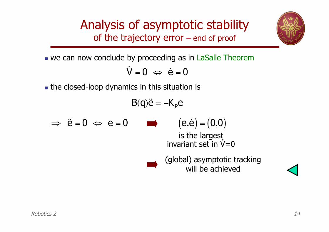
Analysis of asymptotic stability of the trajectory error – end of proof

"  we can now conclude by proceeding as in LaSalle Theorem

!

B(q)˙ ̇ e = "KPe

!

" ˙ ̇ e = 0 # e = 0

!

e, ˙ e ( ) = 0,0( )is the largest

invariant set in V=0 .

Robotics 2 14

!

˙ V = 0 " ˙ e = 0"  the closed-loop dynamics in this situation is

(global) asymptotic tracking will be achieved

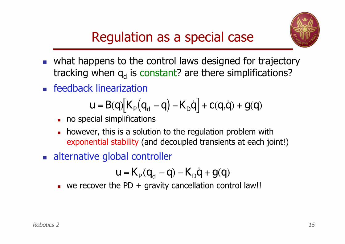
Regulation as a special case

"  what happens to the control laws designed for trajectory tracking when qd is constant? are there simplifications?

"  feedback linearization

"  no special simplifications

"  however, this is a solution to the regulation problem with exponential stability (and decoupled transients at each joint!)

"  alternative global controller

"  we recover the PD + gravity cancellation control law!!

!

u = KP(qd "q) "KD˙ q + g(q)

!

u = B(q) KP qd "q( ) "KD˙ q [ ] + c(q, ˙ q ) + g(q)

Robotics 2 15

Trajectory execution without a model

"  is it possible to accurately reproduce a desired smooth joint-space reference trajectory with reduced or no information on the robot dynamic model?

"  this is feasible in case of repetitive motion tasks over a finite interval of time "  trials are performed iteratively, storing the trajectory error

information of the current execution [k-th iteration] and processing it off line before the next trial [(k+1)-iteration] starts

"  the robot should be reinitialized in the same initial position at the beginning of each trial

"  the control law is made of a non-model based part (typically, a decentralized PD law) + a time-varying feedforward which is updated at every trial

"  this scheme is called iterative trajectory learning Robotics 2 16

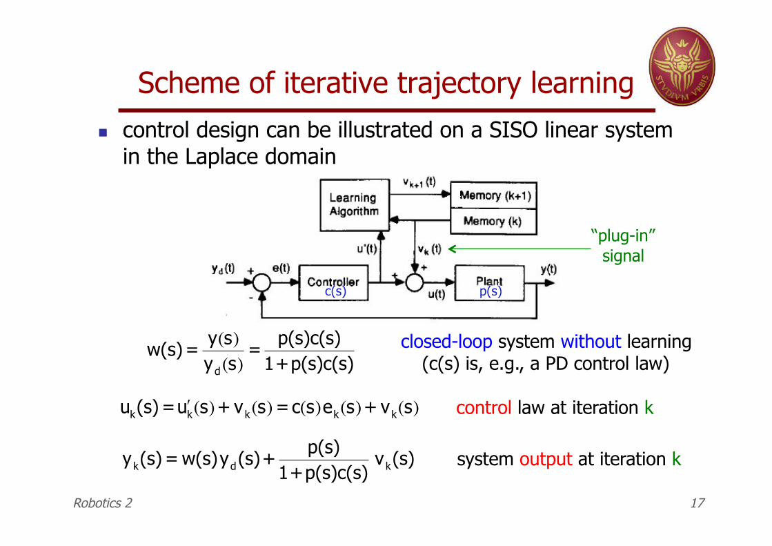
Scheme of iterative trajectory learning

"  control design can be illustrated on a SISO linear system in the Laplace domain

Robotics 2 17

!

w(s)= y(s)yd(s)

= p(s)c(s)1+p(s)c(s)

!

uk(s) = " u k(s)+ vk(s)=c(s)ek(s)+ vk(s)

“plug-in” signal

!

yk(s) = w(s)yd(s)+ p(s)1+p(s)c(s)

vk(s)

closed-loop system without learning (c(s) is, e.g., a PD control law)

control law at iteration k

system output at iteration k

p(s) c(s)

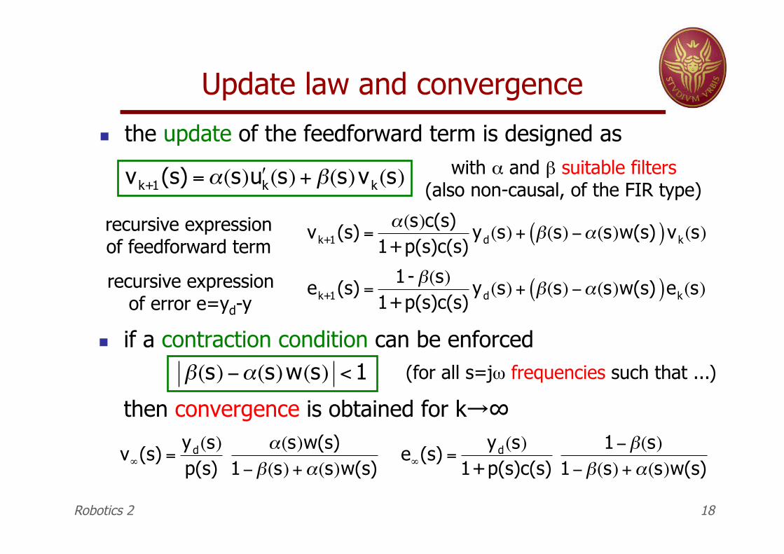
Update law and convergence

"  the update of the feedforward term is designed as

Robotics 2 18

!

vk+1(s) ="(s) # u k(s) + $(s)vk(s)with ! and " suitable filters

(also non-causal, of the FIR type)

recursive expression of feedforward term

recursive expression of error e=yd-y

!

vk+1(s) ="(s)c(s)

1+p(s)c(s)yd(s) + #(s) $"(s)w(s)( )vk(s)

!

ek+1(s) =1- "(s)

1+p(s)c(s)yd(s) + "(s) #$(s)w(s)( )ek(s)

"  if a contraction condition can be enforced

then convergence is obtained for k→"

!

"(s) #$(s)w(s) < 1

!

v"(s) =yd(s)p(s)

#(s)w(s)1$%(s) +#(s)w(s)

!

e"(s) =yd(s)

1+p(s)c(s)1#$(s)

1#$(s) +%(s)w(s)

(for all s=j# frequencies such that ...)

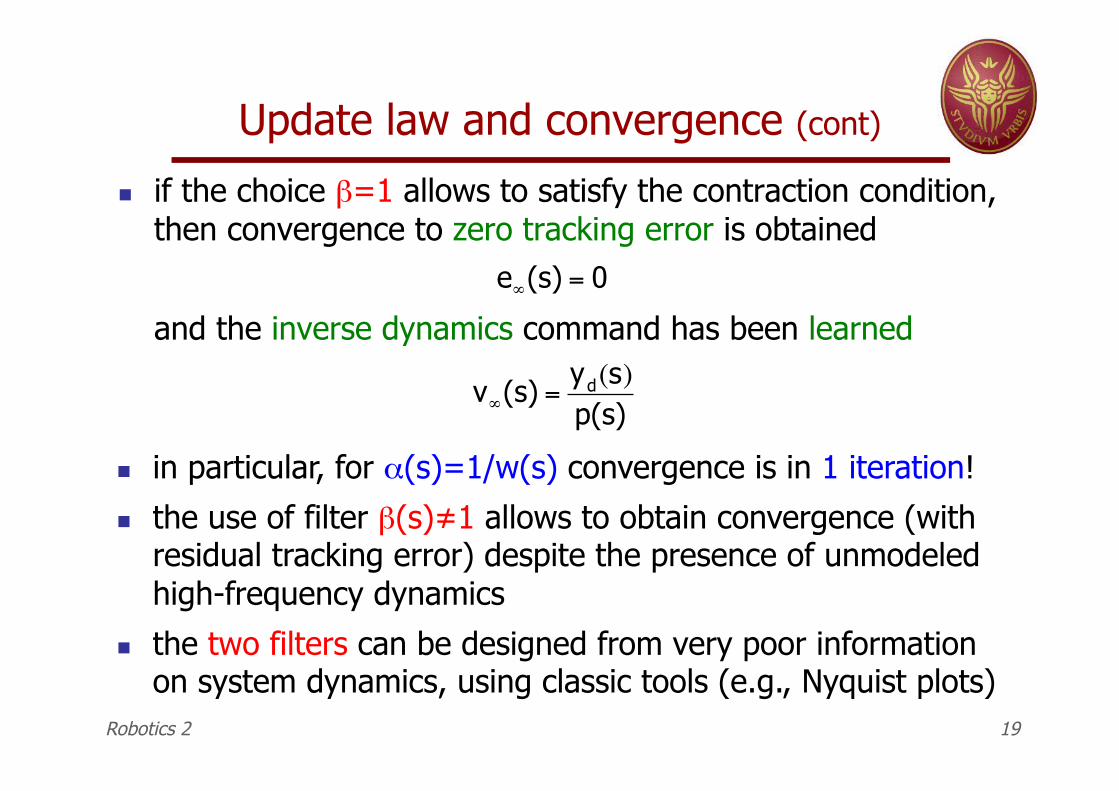
Update law and convergence (cont)

"  if the choice "=1 allows to satisfy the contraction condition, then convergence to zero tracking error is obtained

and the inverse dynamics command has been learned

Robotics 2 19

"  in particular, for !(s)=1/w(s) convergence is in 1 iteration!

"  the use of filter "(s)#1 allows to obtain convergence (with residual tracking error) despite the presence of unmodeled high-frequency dynamics

"  the two filters can be designed from very poor information on system dynamics, using classic tools (e.g., Nyquist plots)

!

v"(s) =yd(s)p(s)

!

e"(s) = 0

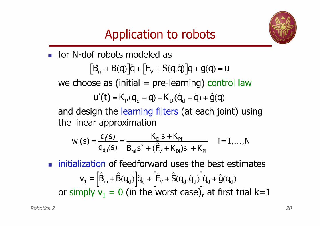
Application to robots

"  for N-dof robots modeled as

we choose as (initial = pre-learning) control law

and design the learning filters (at each joint) using the linear approximation

Robotics 2 20

!

Bm + B(q)[ ]˙ ̇ q + FV + S(q, ˙ q )[ ]˙ q + g(q) = u

!

" u (t) = KP(qd #q) #KD (˙ q d # ˙ q ) + ˆ g (q)

!

wi(s) = qi(s)qd,i(s)

= KDi s +KPiˆ B mi s

2 + ( ˆ F vi +KDi)s +KPi

i=1,…,N

"  initialization of feedforward uses the best estimates

or simply v1 = 0 (in the worst case), at first trial k=1

!

v1 = ˆ B m + ˆ B (qd)[ ]˙ ̇ q d + ˆ F V + ˆ S (qd, ˙ q d)[ ]˙ q d + ˆ g (qd)

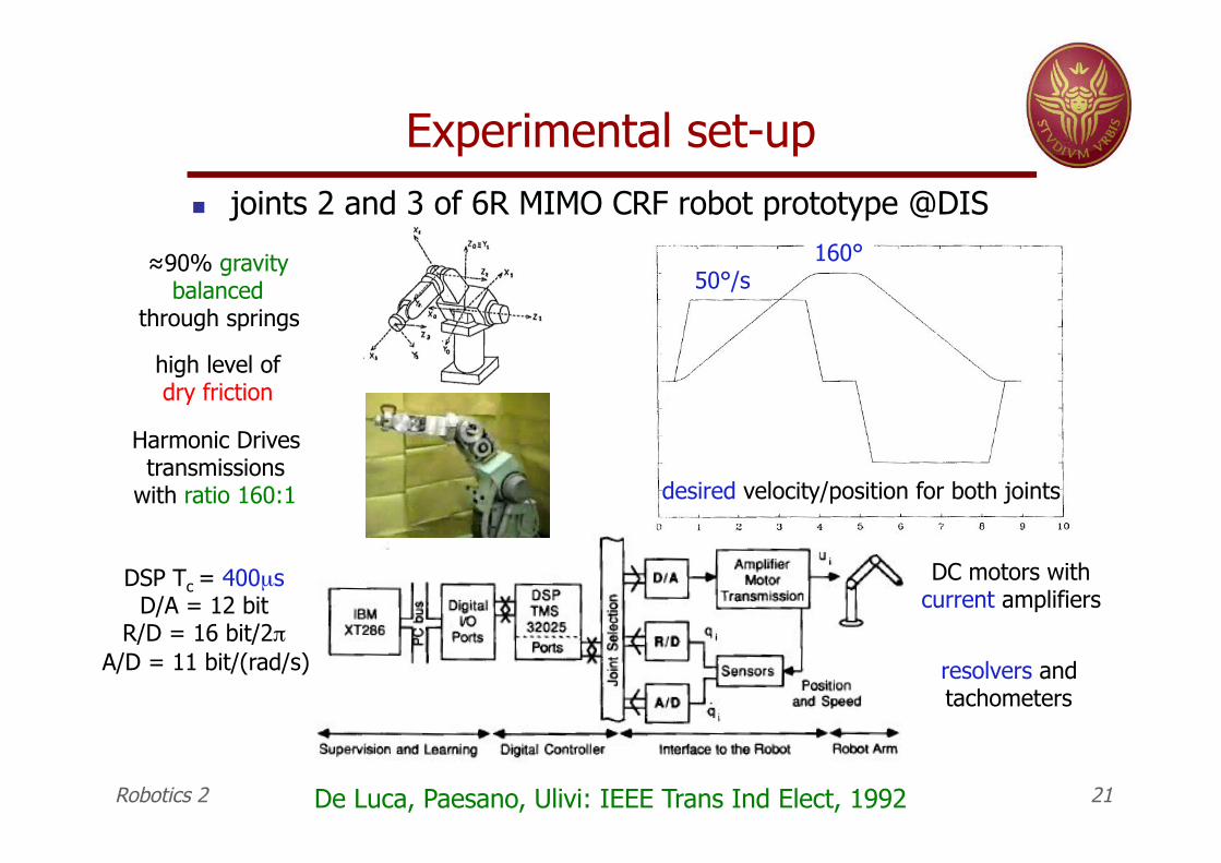
Experimental set-up "  joints 2 and 3 of 6R MIMO CRF robot prototype @DIS

Robotics 2 21

50°/s 160°

desired velocity/position for both joints

$90% gravity balanced

through springs

Harmonic Drives transmissions

with ratio 160:1

resolvers and tachometers

DC motors with current amplifiers

DSP Tc = 400µs D/A = 12 bit

R/D = 16 bit/2$%A/D = 11 bit/(rad/s)%

high level of dry friction

De Luca, Paesano, Ulivi: IEEE Trans Ind Elect, 1992

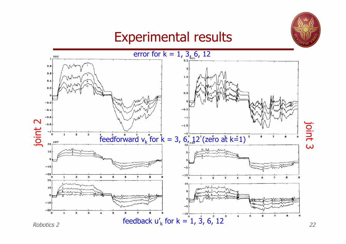
Experimental results

Robotics 2 22

error for k = 1, 3, 6, 12

feedforward vk for k = 3, 6, 12 (zero at k=1) join

t 2

joint 3

feedback u’k for k = 1, 3, 6, 12