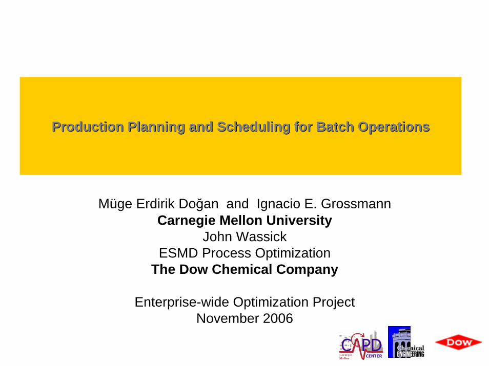
Production Planning and Scheduling for Batch OperationsProduction Planning and Scheduling for Batch Operations

Müge Erdirik Doğan and Ignacio E. GrossmannCarnegie Mellon University

John WassickESMD Process Optimization

The Dow Chemical Company

Enterprise-wide Optimization ProjectNovember 2006

2

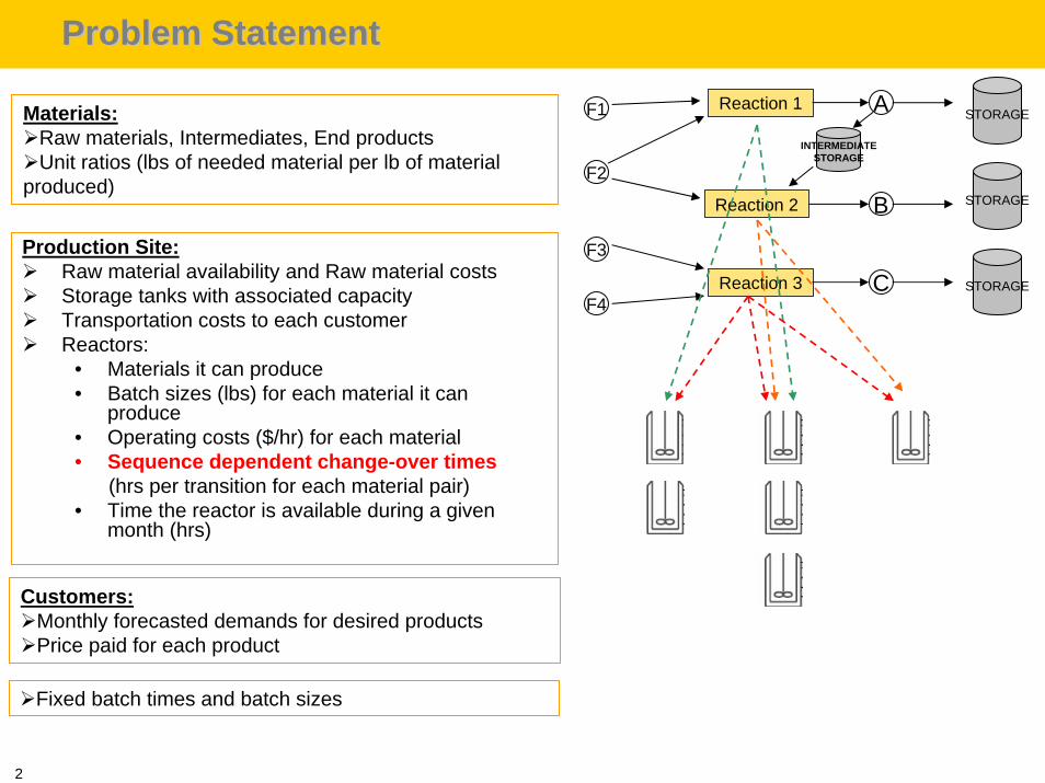
Problem StatementProblem Statement

Production Site:Raw material availability and Raw material costsStorage tanks with associated capacity Transportation costs to each customer Reactors:

• Materials it can produce• Batch sizes (lbs) for each material it can

produce• Operating costs ($/hr) for each material• Sequence dependent change-over times

(hrs per transition for each material pair)• Time the reactor is available during a given

month (hrs)

Customers:Monthly forecasted demands for desired productsPrice paid for each product

Materials:Raw materials, Intermediates, End productsUnit ratios (lbs of needed material per lb of material

produced)

F1

F2

F3

F4

Reaction 1 A

Reaction 2 B

Reaction 3 C

INTERMEDIATESTORAGE

STORAGE

STORAGE

STORAGE

Fixed batch times and batch sizes

3

Problem StatementProblem Statement

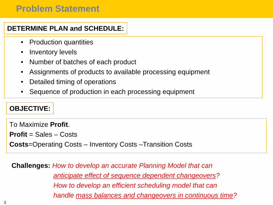
• Production quantities • Inventory levels • Number of batches of each product • Assignments of products to available processing equipment• Detailed timing of operations• Sequence of production in each processing equipment

OBJECTIVE:

To Maximize Profit.Profit = Sales – CostsCosts=Operating Costs – Inventory Costs –Transition Costs

DETERMINE PLAN and SCHEDULE:

Challenges: How to develop an accurate Planning Model that cananticipate effect of sequence dependent changeovers?How to develop an efficient scheduling model that canhandle mass balances and changeovers in continuous time?

4

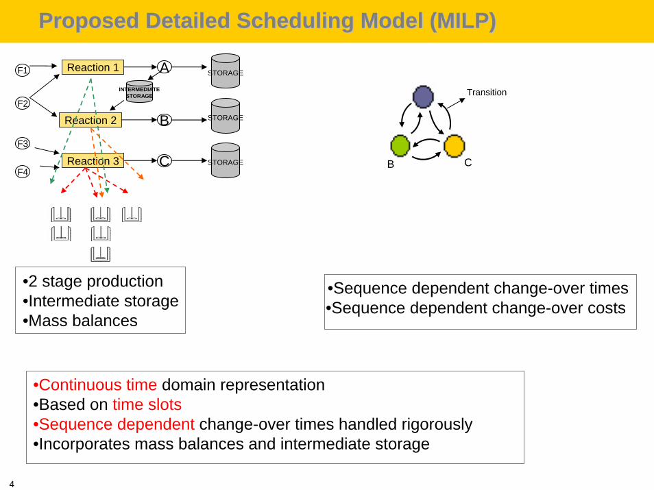
Proposed Detailed Scheduling Model (MILP)Proposed Detailed Scheduling Model (MILP)

•Continuous time domain representation•Based on time slots•Sequence dependent change-over times handled rigorously•Incorporates mass balances and intermediate storage

F1

F2

F3

F4

Reaction 1 A

Reaction 2 B

Reaction 3 C

INTERMEDIATESTORAGE

STORAGE

STORAGE

STORAGE

•2 stage production•Intermediate storage•Mass balances

B C

Transition

•Sequence dependent change-over times•Sequence dependent change-over costs

5

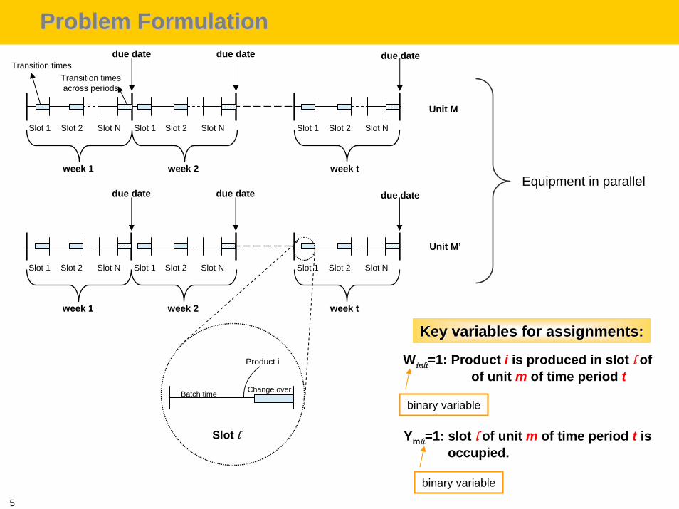
Problem FormulationProblem Formulation

Slot 1 Slot 2 Slot N Slot 1 Slot 2 Slot N Slot 1 Slot 2 Slot N

week 1 week 2 week t

due date due date

Transition timesacross periods

due dateTransition times

Unit M

Slot 1 Slot 2 Slot N Slot 1 Slot 2 Slot N Slot 1 Slot 2 Slot N

week 1 week 2 week t

due date due date due date

Unit M’

Slot l

Batch time Change over

Product i

Key variables for assignments:Key variables for assignments:

Wimlt=1: Product i is produced in slot l of of unit m of time period t

binary variable

Equipment in parallel

Ymlt=1: slot l of unit m of time period t isoccupied.

binary variable

6

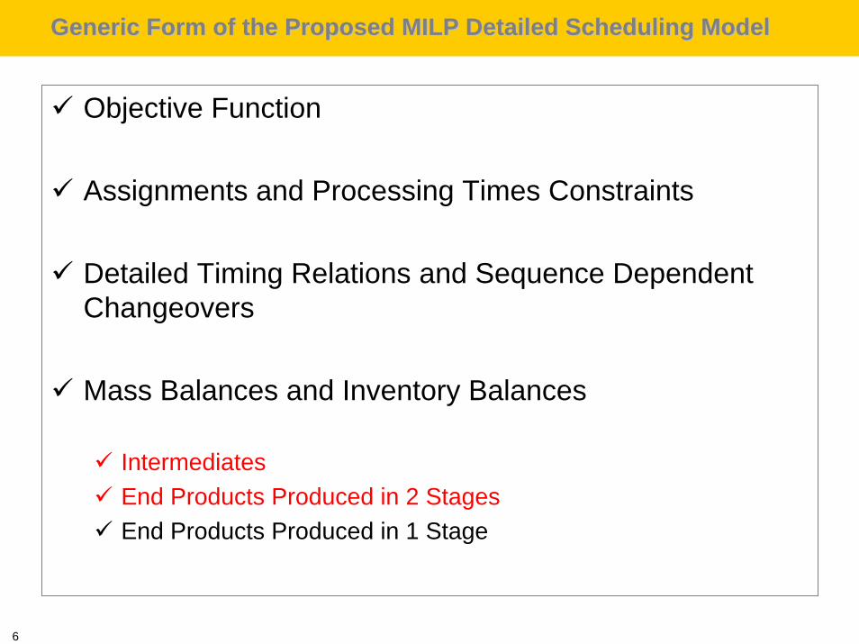
Generic Form of the Proposed MILP Detailed Scheduling ModelGeneric Form of the Proposed MILP Detailed Scheduling Model

Objective Function

Assignments and Processing Times Constraints

Detailed Timing Relations and Sequence Dependent Changeovers

Mass Balances and Inventory Balances

IntermediatesEnd Products Produced in 2 StagesEnd Products Produced in 1 Stage

7

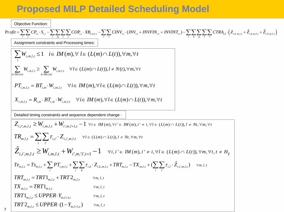
Proposed MILP Detailed Scheduling ModelProposed MILP Detailed Scheduling Model

, , , 1 ( ), ( ( ) ( )), ,i m l ti

W i IM m l L m L t m t≤ ∈ ∀ ∈ ∩ ∀ ∀∑

, , , , , ,( ) ( )

( ( ) ( )), ( ), ,i m l t i m l ti IM m i IM m

W W l L m L t l N t m t∈ ∈

≥ ∀ ∈ ∩ ≠ ∀ ∀∑ ∑

, , , , , , , ( ), ( ( ) ( )), ,i m l t i m i m l tPT BT W i IM m l L m L t m t= ⋅ ∀ ∈ ∀ ∈ ∩ ∀ ∀

, , , , , , , , ( ), ( ( ) ( )), ,i m l t i m i m i m l tX R BT W i IM m l L m L t m t= ⋅ ⋅ ∀ ∈ ∀ ∈ ∩ ∀ ∀

, ', , , , , , ', ,'1', 1 , ' ( ), ' , ( ( ) ( )), , ,1i i m l t i m l t i m t i i IM m i i l L m L t m t t HtZ W W + ∀ ∈ ≠ ∀ ∈ ∩ ∀ ∀ ≠≥ + −%

, , , , , , , , , , , , , , , , , ' , ', , ,'

, ,ˆ( )m l t m l t i m l t i k i k m l t m l t m l t i i i i m l ti i k i i

m l tTe Ts PT Z TRT TX Zτ τ ∀= + + ⋅ + − + ⋅∑ ∑∑ ∑∑

, ', , , , , , ', , 1, ( ), ' ( ), ' , ( ( ) ( )), , ,1i i m l t i m l t i m l t i IM m i IM m i i l L m L t l Nt m tZ W W + ∀ ∈ ∀ ∈ ≠ ∀ ∈ ∩ ≠ ∀ ∀≥ + −

, , , ' , ', , ,'

( ( ) ( )), , ,m l t i i i i m l ti i

l L m L t l Nt m tTR Zτ ∀ ∈ ∩ ≠ ∀ ∀= ⋅∑∑

, , , , , ,

, , , ,

, , , 1,

, , , 1,

, ,

, ,

, ,

, ,

1 21

12 (1 )

m l t m l t m l t

m l t m l t

m l t m l t

m l t m l t

m l t

m l t

m l t

m l t

TRT TRT TRTTX TRTTRT UPPER YTRT UPPER Y

+

+

∀

∀

∀

∀

= +

=

≤ ⋅

≤ ⋅ −

( ), , , , , , , , , , , , , , , , , , , , , , ,ˆPr ( )i t i t i t i m l t i t i t i t i t i k i k m l t i k m l t i k m l t

i t i m l t i t i k m l t

ofit CP S COP XB CINV INV INVFIN INVINT CTRA Z Z Z= ⋅ − ⋅ − ⋅ + + − ⋅ + +∑∑ ∑∑∑∑ ∑∑ ∑∑∑∑∑ %

Assignment constraints and Processing times:

Detailed timing constraints and sequence dependent change :

Objective Function:

8

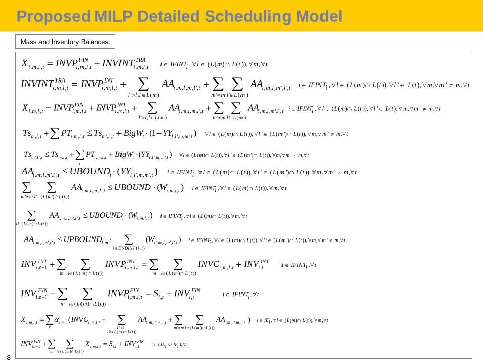
, , , , , , , , , , ( ( ) ( )), ,FIN TRA

i m l t i m l t i m l t i IFINT l L m L t m tiX INVP INVINT ∈ ∀ ∈ ∩ ∀ ∀= +

, , , , ' ', , , , , '', , , , ', ', , ,' '' ' ' ( ( ') ( ))

' ( ( ) ( ))

, ( ( ) ( )), ,( )i m l t i i i m l t i m l m l t i m l m l ti l l m m l L m L t

l L m L t

i IE l L m L t m tiX INVC AA AAα< ≠ ∈ ∩

∈ ∩

∈ ∀ ∈ ∩ ∀ ∀= ⋅ + +∑ ∑ ∑ ∑

, , , , , , , , , , ', , , , ', ',' , ' ( ) ' ' ( ')

, ( ( ) ( )), ' ( ), , ' ,TRA INT

i m l t i m l t i m l m l t i m l m l tl l l L m m m l L m

i IFINT l L m L t l L t m m m tiINVINT INVP AA AA> ∈ ≠ ∈

∈ ∀ ∈ ∩ ∀ ∈ ∀ ∀ ≠ ∀= + +∑ ∑ ∑, , , , , , , , , , , , , ', , , , ', ',

' , ' ( ) ' ' ( ')

, ( ( ) ( )), ' ( ), , ' ,FIN INT

i m l t i m l t i m l t i m l m l t i m l m l tl l l L m m m l L m

i IFINT l L m L t l L t m m m tiX INVP INVP AA AA> ∈ ≠ ∈

∈ ∀ ∈ ∩ ∀ ∈ ∀ ∀ ≠ ∀= + + +∑ ∑ ∑

, , , , , ', ', , ', , ', ( ( ) ( )), ' ( ( ') ( )), , ' ,(1 )m l t i m l t m l t t l l m m ti

l L m L t l L m L t m m m tTs PT Ts BigW YY ∀ ∈ ∩ ∀ ∈ ∩ ∀ ∀ ≠ ∀+ ≤ + ⋅ −∑

', ', , , , , , , ', , ', ( ( ) ( )), ' ( ( ') ( )), , ' ,( )m l t m l t i m l t t l l m m ti

l L m L t l L m L t m m m tTs Ts PT BigW YY ∀ ∈ ∩ ∀ ∈ ∩ ∀ ∀ ≠ ∀≤ + + ⋅∑, , , ', ', , ', , ', , ( ( ) ( )), ' ( ( ') ( )), , ' ,( )i m l m l t i l l m m t i IFINT l L m L t l L m L t m m m tiAA UBOUND YY ∈ ∀ ∈ ∩ ∀ ∈ ∩ ∀ ∀ ≠ ∀≤ ⋅

, , , ', ', , , ,' ' ( ( ') ( ))

, ( ( ) ( )), ,( )i m l m l t i i m l tm m l L m L t

i IFINT l L m L t m tiAA UBOUND W≠ ∈ ∩

∈ ∀ ∈ ∩ ∀ ∀≤ ⋅∑ ∑

, , , ', ', , , ,' ( ( ) ( ))

, ( ( ) ( )), ,( )i m l m l t i i m l tl L m L t

i IFINT l L m L t m tiAA UBOUND W∈ ∩

∈ ∀ ∈ ∩ ∀ ∀≤ ⋅∑

, , , ', ', , ', , , ', ',' ( ', )

, ( ( ) ( )), ' ( ( ') ( )), , ' ,( )i m l m l t i m i m l m l ti ENDINT i i

i IFINT l L m L t l L m L t m m m tiAA UPBOUND W∈

∈ ∀ ∈ ∩ ∀ ∈ ∩ ∀ ∀ ≠ ∀≤ ⋅ ∑

, 1 , , , , , , ,( ( ) ( )) ( ( ) ( ))

,INT INT INT

i t i m l t i m l t i tm l L m L t m l L m L t

i IFINT tiINV INVP INVC INV−∈ ∩ ∈ ∩

∈ ∀+ = +∑ ∑ ∑ ∑

, 1 , , , , ,( ( ) ( ))

,FIN FIN FIN

i t i m l t i t i tm l L m L t

i IFINT tiINV INVP S INV−∈ ∩

∈ ∀+ = +∑ ∑

, 1 , , , , ,( ( ) ( ))

( ),FIN FIN

i t i m l t i t i tm l L m L t

i IE IF ti iINV X S INV−∈ ∩

∈ ∪ ∀+ = +∑ ∑

Mass and Inventory Balances:

ProposedProposed MILP Detailed Scheduling ModelMILP Detailed Scheduling Model

9

RemarksRemarks

Very large scale modelSolution times quickly intractable

Number of slots unknown prior to solving the modelHandling mass balances for products produced in 2 stageDetailed timing constraints introduced for handling sequence dependent change-overs

To overcome these difficulties, we introduce a bi-level decomposition scheme

10

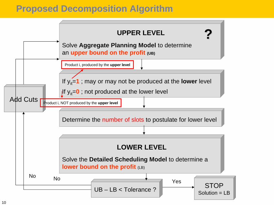
Proposed Decomposition AlgorithmProposed Decomposition Algorithm

Solve Aggregate Planning ModelAggregate Planning Model to determine an upper bound on the profit (UB)

UPPER LEVEL

Yes

Solve the Detailed Scheduling ModelDetailed Scheduling Model to determine a lower bound on the profit (LB)

LOWER LEVEL

UB – LB < Tolerance ?

If yit=1 ; may or may not be produced at the lower level

If yit=0 ; not produced at the lower level

STOPSolution = LB

No

Add Cuts

No

Product i, produced by the upper level

Product i, NOT produced by the upper level

Determine the number of slots to postulate for lower level

??

11

Proposed MILP Planning ModelProposed MILP Planning Model

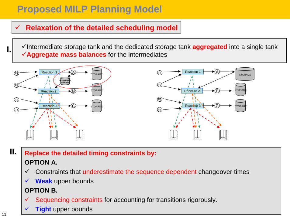
Relaxation of the detailed scheduling model

Intermediate storage tank and the dedicated storage tank aggregated into a single tank Aggregate mass balances for the intermediates

F1

F2

F3

F4

Reaction 1 A

Reaction 2 B

Reaction 3 C

INTERMEDIATESTORAGE

STORAGE

STORAGE

STORAGE

STORAGEF1

F2

F3

F4

Reaction 1 A

Reaction 2 B

Reaction 3 C

STORAGE

STORAGE

I.

Replace the detailed timing constraints by:OPTION A.

Constraints that underestimate the sequence dependent changeover timesWeak upper bounds

OPTION B.Sequencing constraints for accounting for transitions rigorously.Tight upper bounds

II.

12

Generic Form of the Proposed MILP Planning ModelGeneric Form of the Proposed MILP Planning Model

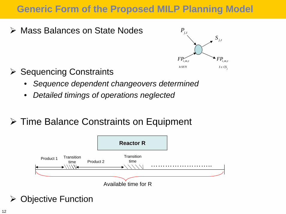
Mass Balances on State Nodes

Sequencing Constraints• Sequence dependent changeovers determined• Detailed timings of operations neglected

Time Balance Constraints on Equipment

Objective Function

,j tP,j tS

, ,i m tFP , ,i m tFPSETOI∈

jI CS∈

Reactor RReactor R

Available time for R

Product 1 TransitiontimeProduct 2

Transitiontime ……………………..

13

Key Variables for the ModelKey Variables for the Model

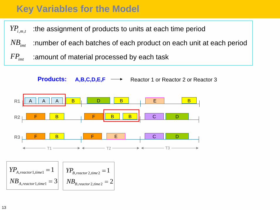
, ,i m tYP :the assignment of products to units at each time period

imtNB :number of each batches of each product on each unit at each period

imtFP :amount of material processed by each task

A,B,C,D,E,F Reactor 1 or Reactor 2 or Reactor 3Products:

T1 T2 T3

F B F C DR3 E

R2 F B F C DB B

D B BR1 AA A B E

, 1, 1

, 1, 1

1

3A reactor time

A reactor time

YP

NB

=

=, 2, 2

, 2, 2

1

2B reactor time

B reactor time

YP

NB

=

=

14

Proposed Planning ModelProposed Planning Model

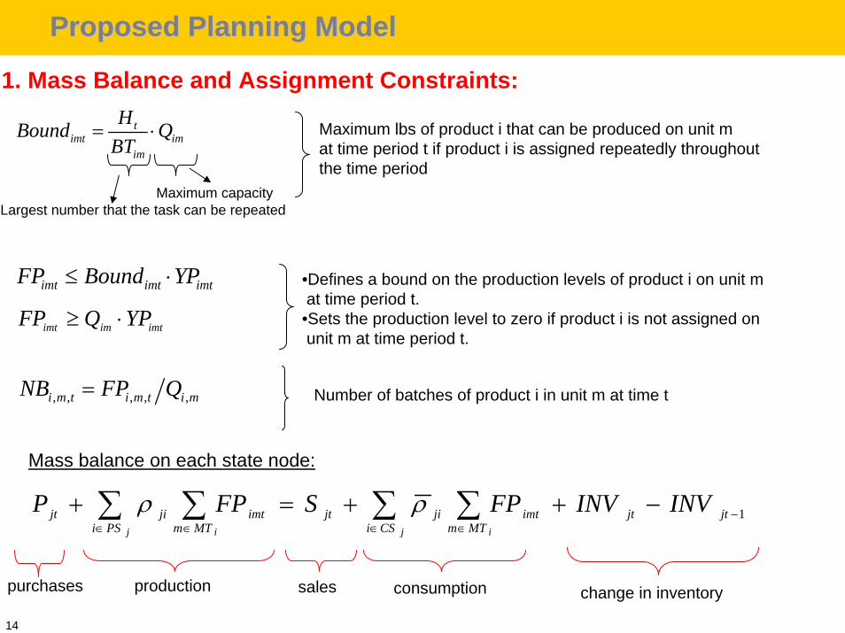
1. Mass Balance and Assignment Constraints:

imt imt imtFP Bound YP≤ ⋅

imtimimt YPQFP ⋅≥

•Defines a bound on the production levels of product i on unit mat time period t.

•Sets the production level to zero if product i is not assigned onunit m at time period t.

Largest number that the task can be repeated

timt im

im

HBound QBT

= ⋅

Maximum capacity

Maximum lbs of product i that can be produced on unit mat time period t if product i is assigned repeatedly throughoutthe time period

, , , , ,i m t i m t i mNB FP Q= Number of batches of product i in unit m at time t

∑ ∑∑ ∑∈

−∈∈ ∈

−++=+j ij i CSi

jtjtMTm

imtjiPSi

jtMTm

imtjijt INVINVFPSFPP 1ρρ

purchases production sales consumption change in inventory

Mass balance on each state node:

15

Proposed Planning ModelProposed Planning Model

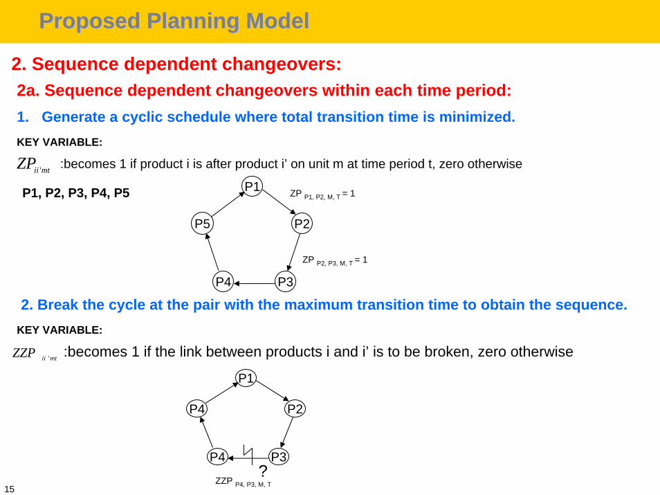
2. Sequence dependent changeovers:2a. Sequence dependent changeovers within each time period:1. Generate a cyclic schedule where total transition time is minimized.KEY VARIABLE:

mtiiZP ' :becomes 1 if product i is after product i’ on unit m at time period t, zero otherwise

P1, P2, P3, P4, P5 P1

P2

P3

ZP P1, P2, M, T = 1

ZP P2, P3, M, T = 1

2. Break the cycle at the pair with the maximum transition time to obtain the sequence.

mtiiZZP ' :becomes 1 if the link between products i and i’ is to be broken, zero otherwise KEY VARIABLE:

P1

P2

P3P4

P4

?ZZP P4, P3, M, T

P4

P4P5

16

Proposed Planning ModelProposed Planning Model

P1

P2

P3P4

P4

P2, P3, P4, P5, P1 ZZP P1, P2, M, T = 1

P3, P4, P5, P1, P2 ZZP P2, P3, M, T = 1

P4, P5, P1, P2, P3 ZZP P3, P4, M, T = 1

P5, P1, P2, P3, P4 ZZP P4, P5, M, T = 1

P1, P2, P3, P4, P5 ZZP P5, P1, M, T = 1

P1

P2

P3P4

P4

P2, P3, P4, P5, P1 ZZP P1, P2, M, T = 1

P3, P4, P5, P1, P2 ZZP P2, P3, M, T = 1

P4, P5, P1, P2, P3 ZZP P3, P4, M, T = 1

P5, P1, P2, P3, P4 ZZP P4, P5, M, T = 1

P1, P2, P3, P4, P5 ZZP P5, P1, M, T = 1

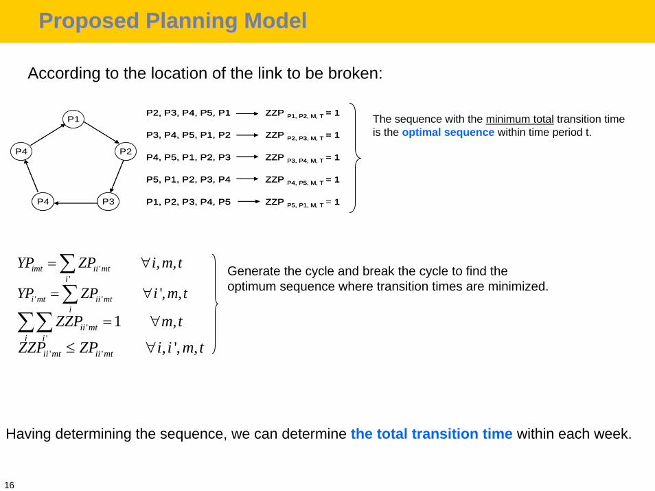
According to the location of the link to be broken:

The sequence with the minimum total transition time is the optimal sequence within time period t.

''

, ,imt ii mti

YP ZP i m t= ∀∑' ' ', ,i mt ii mt

i

YP ZP i m t= ∀∑'

'1 ,ii mt

i iZZP m t= ∀∑∑

' ' , ', ,ii mt ii mtZZP ZP i i m t≤ ∀

Generate the cycle and break the cycle to find theoptimum sequence where transition times are minimized.

Having determining the sequence, we can determine the total transition time within each week.

17

Proposed Planning ModelProposed Planning Model

, , ' , ', , , ' , ', ,' '

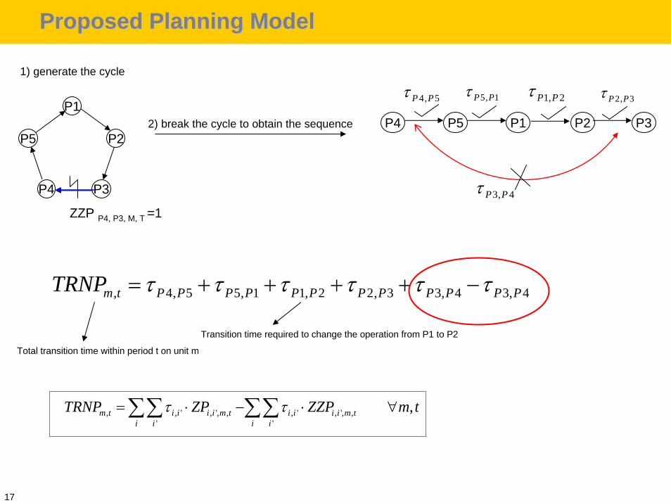
,m t i i i i m t i i i i m ti i i i

TRNP ZP ZZP m tτ τ= ⋅ − ⋅ ∀∑∑ ∑∑

P4 P5 P1 P2 P3

4, 5P Pτ 5, 1P Pτ 1, 2P Pτ 2, 3P Pτ

3, 4P Pτ

P1

P2

P3P4

P5

ZZP P4, P3, M, T =1

1) generate the cycle

2) break the cycle to obtain the sequence

Total transition time within period t on unit m

, 4, 5 5, 1 1, 2 2, 3 3, 4 3, 4m t P P P P P P P P P P P PTRNP τ τ τ τ τ τ= + + + + −

Transition time required to change the operation from P1 to P2

18

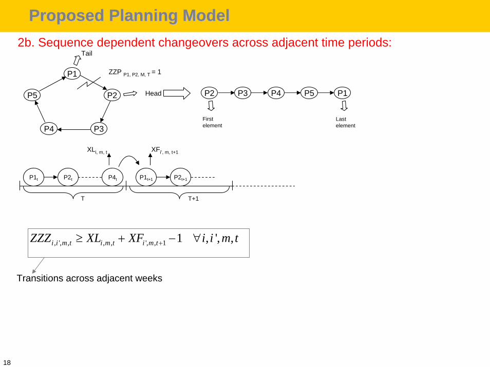
Proposed Planning ModelProposed Planning Model2b. Sequence dependent changeovers across adjacent time periods:

P1

P2

P3P4

P5

ZZP P1, P2, M, T = 1

Tail

Head P2 P3 P4 P5 P1

First element

Last element

XLi, m, t

P1t P2t P4t P1t+1 P2t+1

XFi’, m, t+1

T T+1

, ', , , , ', , 1 1 , ', ,i i m t i m t i m tZZZ XL XF i i m t+≥ + − ∀

Transitions across adjacent weeks

19

Proposed Planning ModelProposed Planning Model

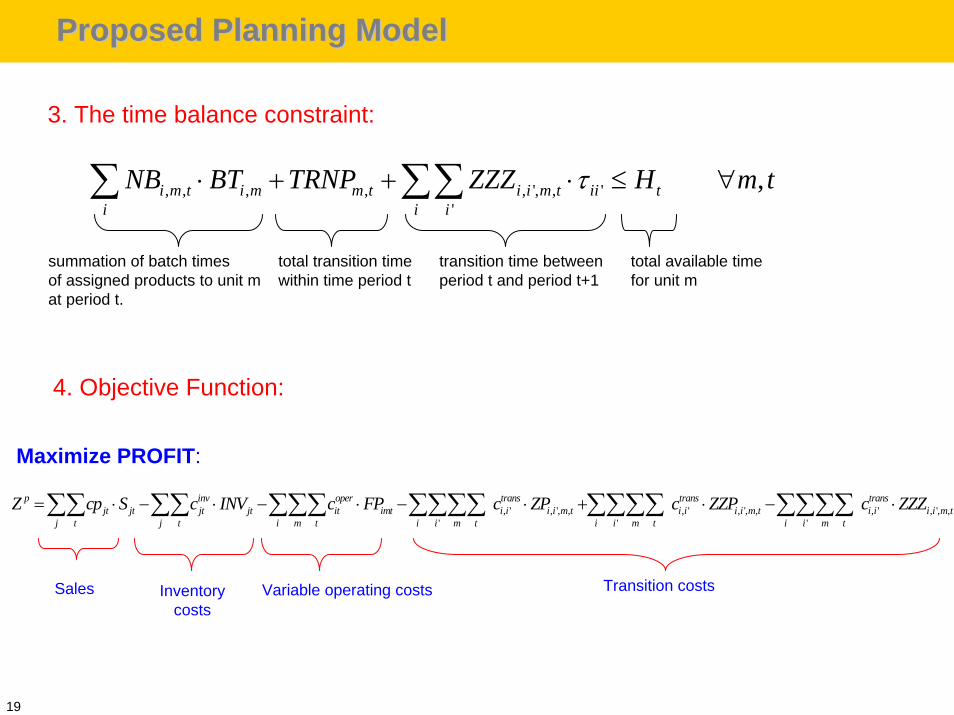
3. The time balance constraint:

, , , , , ', , ''

,i m t i m m t i i m t ii ti i i

NB BT TRNP ZZZ H m tτ⋅ + + ⋅ ≤ ∀∑ ∑∑

summation of batch timesof assigned products to unit mat period t.

total transition timewithin time period t

transition time betweenperiod t and period t+1

total available timefor unit m

, ' , ', , , ' , ', , , ' , ', ,' ' '

p inv oper trans trans transjt jt jt jt it imt i i i i m t i i i i m t i i i i m t

j t j t i m t i i m t i i m t i i m tZ cp S c INV c FP c ZP c ZZP c ZZZ= ⋅ − ⋅ − ⋅ − ⋅ + ⋅ − ⋅∑∑ ∑∑ ∑∑∑ ∑∑∑∑ ∑∑∑∑ ∑∑∑∑

Sales Inventorycosts

Transition costsVariable operating costs

Maximize PROFIT:

4. Objective Function:

20

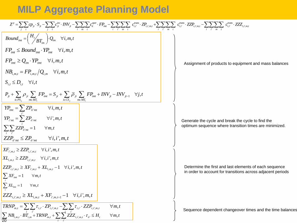
MILP Aggregate Planning ModelMILP Aggregate Planning Model

, ,imt imt imtFP Bound YP i m t≤ ⋅ ∀

, ,imt im imtFP Q YP i m t≥ ⋅ ∀

, , , , , , ,i m t i m t i mNB FP Q i m t= ∀

1 ,j i j i

jt ji imt jt ji imt jt jti PS m MT i CS m MT

P FP S FP INV INV j tρ ρ −∈ ∈ ∈ ∈

+ = + + − ∀∑ ∑ ∑ ∑

, ,timt im

im

HBound Q i m tBT⎛ ⎞= ⋅ ∀⎜ ⎟⎝ ⎠

, , ,i t i tS D i t≤ ∀

Generate the cycle and break the cycle to find theoptimum sequence where transition times are minimized.

, ', , , , ', , 1 1 , ', ,i i m t i m t i m tZZZ XL XF i i m t+≥ + − ∀

', , , ', , , ', ,i m t i i m tXF ZZP i i m t≥ ∀

, , , ', , , ', ,i m t i i m tXL ZZP i i m t≥ ∀

, ', , ', , , , 1 , ', ,i i m t i m t i m tZZP XF XL i i m t≥ + − ∀

1 ,imti

XF m t= ∀∑1 ,imt

iXL m t= ∀∑

''

, ,imt ii mti

YP ZP i m t= ∀∑' ' ', ,i mt ii mt

i

YP ZP i m t= ∀∑'

'1 ,ii mt

i iZZP m t= ∀∑∑

' ' , ', ,ii mt ii mtZZP ZP i i m t≤ ∀

, , ' , ', , , ' , ', ,' '

,m t i i i i m t i i i i m ti i i i

TRNP ZP ZZP m tτ τ= ⋅ − ⋅ ∀∑∑ ∑∑, , , , , ', , '

',i m t i m m t i i m t ii t

i i iNB BT TRNP ZZZ H m tτ⋅ + + ⋅ ≤ ∀∑ ∑∑

, ' , ', , , ' , ', , , ' , ', ,' ' '

p inv oper trans trans transjt jt jt jt it imt i i i i m t i i i i m t i i i i m t

j t j t i m t i i m t i i m t i i m tZ cp S c INV c FP c ZP c ZZP c ZZZ= ⋅ − ⋅ − ⋅ − ⋅ + ⋅ − ⋅∑∑ ∑∑ ∑∑∑ ∑∑∑∑ ∑∑∑∑ ∑∑∑∑

Determine the first and last elements of each sequencein order to account for transitions across adjacent periods

Sequence dependent changeover times and the time balances

Assignment of products to equipment and mass balances

21

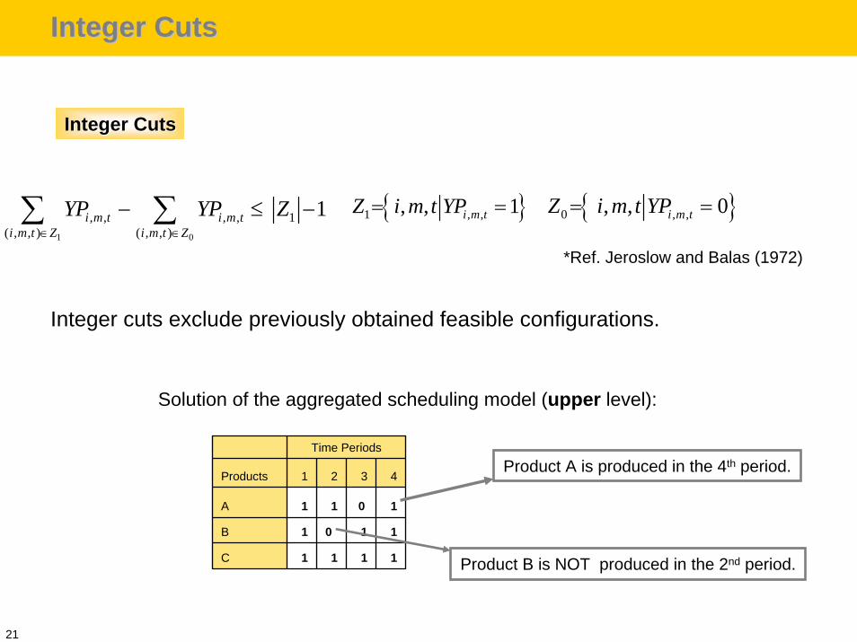
Integer CutsInteger Cuts

1 0

, , , , 1( , , ) ( , , )

1i m t i m ti m t Z i m t Z

YP YP Z∈ ∈

− ≤ −∑ ∑ { }1 , ,, , 1i m tZ i m t YP= =

Integer CutsInteger Cuts

{ }0 , ,, , 0i m tZ i m t YP= =

Integer cuts exclude previously obtained feasible configurations.

*Ref. Jeroslow and Balas (1972)

Solution of the aggregated scheduling model (upper level):

Time Periods

Products 1 2 3 4

A 1 1 0 1

B 1 0 1 1

C 1 1 1 1

Product A is produced in the 4th period.

Product B is NOT produced in the 2nd period.

22

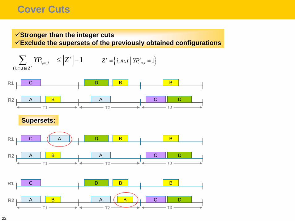
Cover CutsCover Cuts

Stronger than the integer cutsStronger than the integer cutsExclude the supersets of the previously obtained configurationsExclude the supersets of the previously obtained configurations

, ,( , , )

1r

ri m t

i m t Z

YP Z∈

≤ −∑ { }, ,, , 1r ri m tZ i m t YP= =

A

D

B

C B

A C D

B

T1 T2 T3

R1

R2

A

A

D

B

C B

A C D

B

T1 T2 T3

R1

R2

A

D

B

C B

A C D

B

T1 T2 T3

R1

R2 B

Supersets:Supersets:

23

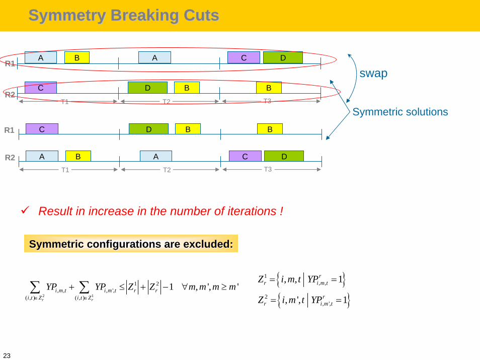
Symmetry Breaking CutsSymmetry Breaking Cuts

T1 T2 T3

A

D

B

C B

A C D

B

R1

R2

A

D

B

C B

A C D

B

T1 T2 T3

R1

R2

swap

Symmetric solutions

Result in increase in the number of iterations !

2 1

1 2, , , ',

( , ) ( , )

1 , ', 'r r

i m t i m t r ri t Z i t Z

YP YP Z Z m m m m∈ ∈

+ ≤ + − ∀ ≥∑ ∑ { }{ }

1, ,

2, ',

, , 1

, ', 1

rr i m t

rr i m t

Z i m t YP

Z i m t YP

= =

= =

Symmetric configurations are excluded:Symmetric configurations are excluded:

24

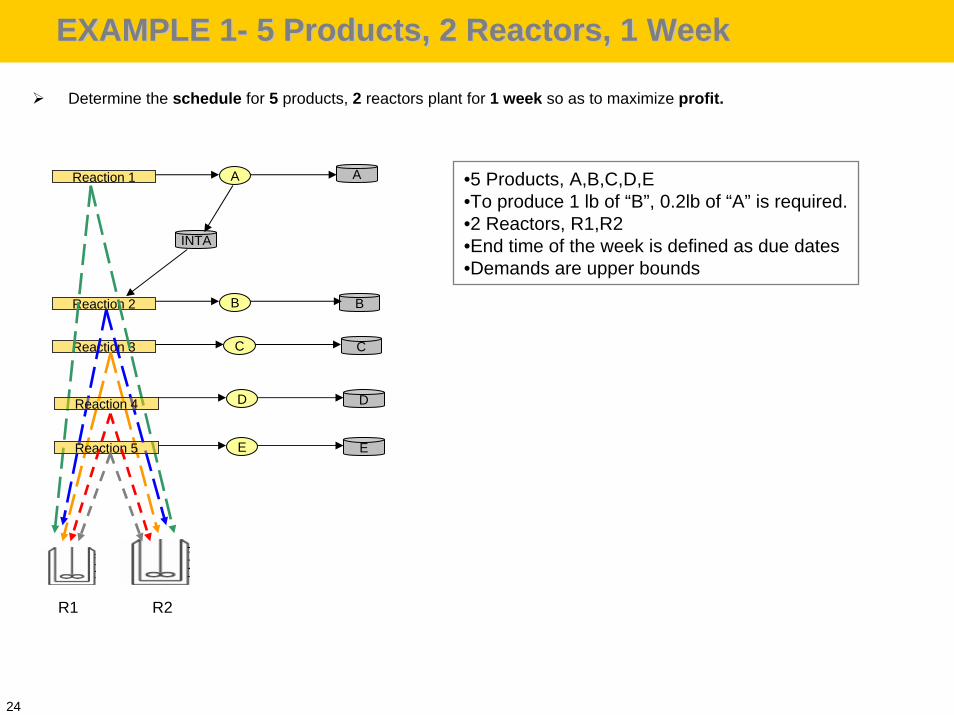
EXAMPLE 1EXAMPLE 1-- 5 Products, 2 Reactors, 1 Week5 Products, 2 Reactors, 1 Week

Determine the schedule for 5 products, 2 reactors plant for 1 week so as to maximize profit.

•5 Products, A,B,C,D,E•To produce 1 lb of “B”, 0.2lb of “A” is required.•2 Reactors, R1,R2•End time of the week is defined as due dates•Demands are upper bounds

Reaction 1

Reaction 2

Reaction 3

A

B

C

R1 R2

A

B

C

INTA

Reaction 4 DD

Reaction 5 EE

25

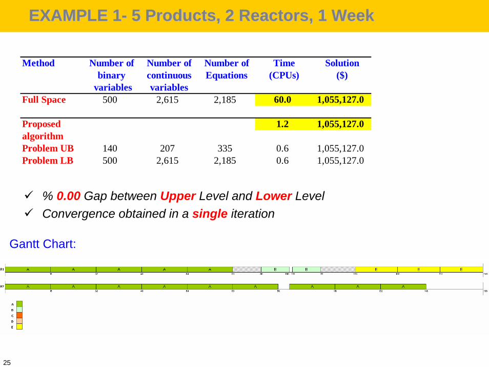
EXAMPLE 1EXAMPLE 1-- 5 Products, 2 Reactors, 1 Week 5 Products, 2 Reactors, 1 Week

Method Number of Number of Number of Time Solutionbinary continuous Equations (CPUs) ($)

variables variablesFull Space 500 2,615 2,185 60.0 1,055,127.0

Proposed 1.2 1,055,127.0algorithmProblem UB 140 207 335 0.6 1,055,127.0Problem LB 500 2,615 2,185 0.6 1,055,127.0

Gantt Chart:

% 0.00 Gap between Upper Level and Lower LevelConvergence obtained in a single iteration

26

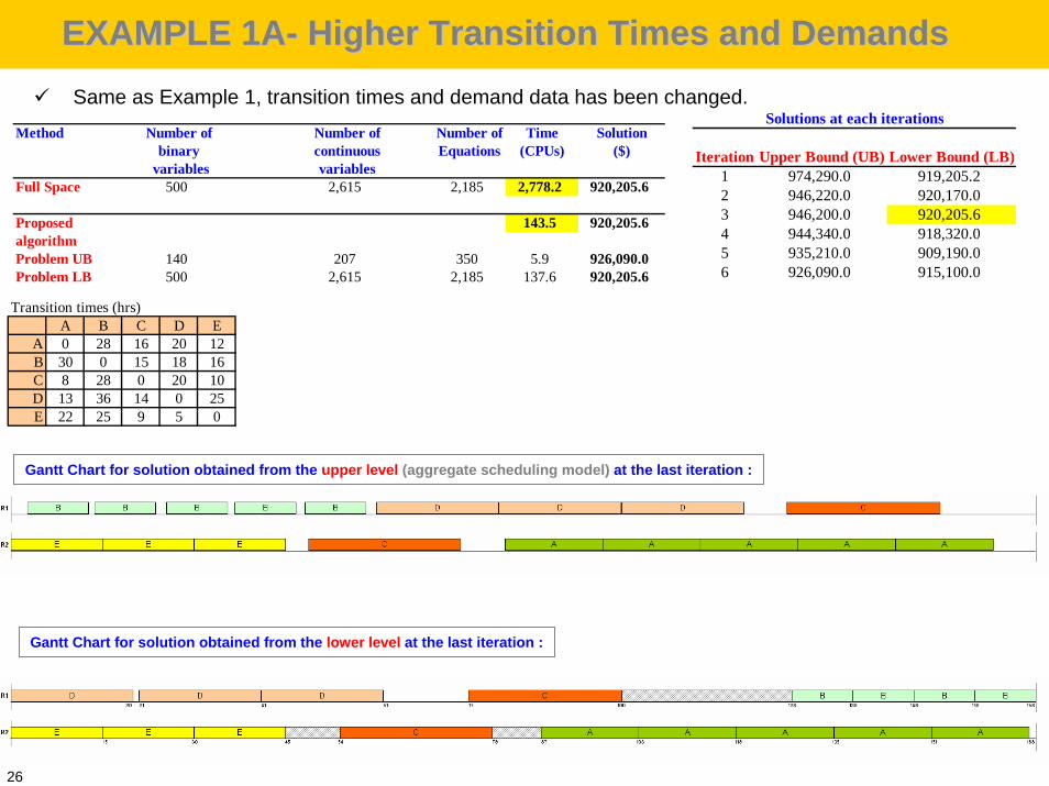
EXAMPLE 1AEXAMPLE 1A-- Higher Transition Times and DemandsHigher Transition Times and DemandsSame as Example 1, transition times and demand data has been changed.

Method Number of Number of Number of Time Solutionbinary continuous Equations (CPUs) ($)

variables variablesFull Space 500 2,615 2,185 2,778.2 920,205.6

Proposed 143.5 920,205.6algorithmProblem UB 140 207 350 5.9 926,090.0Problem LB 500 2,615 2,185 137.6 920,205.6

Solutions at each iterations

pper Bound (UB) Lower Bound (LB)974,290.0 919,205.2946,220.0 920,170.0946,200.0 920,205.6944,340.0 918,320.0935,210.0 909,190.0926,090.0 915,100.0

Iteration U123456

Transition times (hrs)A B C D E

A 0 28 16 20 12B 30 0 15 18 16C 8 28 0 20 10D 13 36 14 0 25E 22 25 9 5 0

Gantt Chart for solution obtained from the upper level (aggregate scheduling model) at the last iteration :

Gantt Chart for solution obtained from the lower level at the last iteration :

27

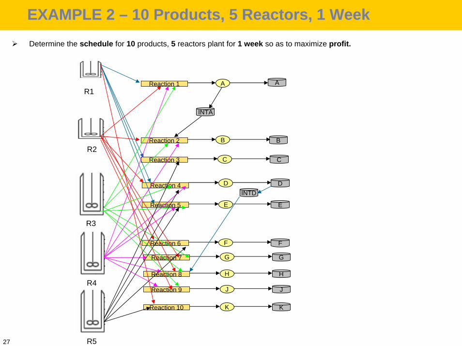
EXAMPLE 2 EXAMPLE 2 –– 10 Products, 5 Reactors, 1 Week10 Products, 5 Reactors, 1 Week

Reaction 1

Reaction 2

Reaction 3

A

B

C

R1

R2

A

B

C

INTA

Reaction 4 DD

Reaction 5 EE

Reaction 6 FF

R3

R4

INTD

Reaction 7 GG

Reaction 8 HH

Reaction 9 JJ

Reaction 10 KK

R5

Determine the schedule for 10 products, 5 reactors plant for 1 week so as to maximize profit.

28

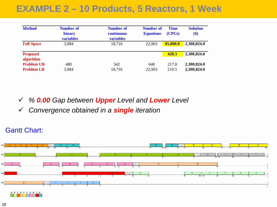
EXAMPLE 2 EXAMPLE 2 –– 10 Products, 5 Reactors, 1 Week10 Products, 5 Reactors, 1 Week

Gantt Chart:

Method Number of Number of Number of Time Solutionbinary continuous Equations (CPUs) ($)

variables variablesFull Space 3,984 18,716 22,903 85,000.0 2,300,824.0

Proposed 428.3 2,300,824.0algorithmProblem UB 480 542 648 217.8 2,300,824.0Problem LB 3,984 18,716 22,903 210.5 2,300,824.0

% 0.00 Gap between Upper Level and Lower LevelConvergence obtained in a single iteration

29

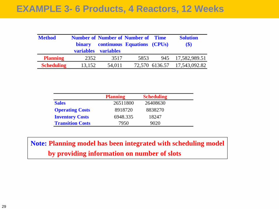
EXAMPLE 3EXAMPLE 3-- 6 Products, 4 Reactors, 12 Weeks6 Products, 4 Reactors, 12 Weeks

Method Number of Number of Number of Time Solutionbinary continuous Equations (CPUs) ($)

variables variablesPlanning 2352 3517 5853 945 17,582,989.51

Scheduling 13,152 54,011 72,570 6136.57 17,543,092.82

Planning SchedulingSales 26511800 26408630Operating Costs 8918720 8838270Inventory Costs 6948.335 18247Transition Costs 7950 9020

Note: Planning model has been integrated with scheduling modelby providing information on number of slots

30

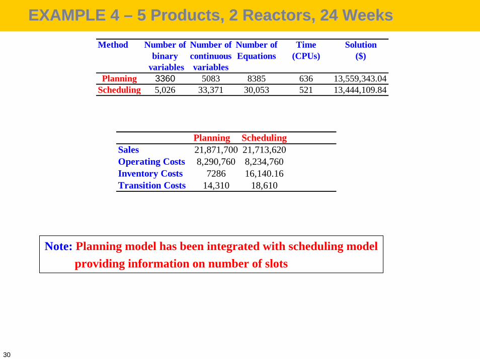
EXAMPLE 4 EXAMPLE 4 –– 5 Products, 2 Reactors, 24 Weeks5 Products, 2 Reactors, 24 WeeksMethod Number of Number of Number of Time Solution

binary continuous Equations (CPUs) ($)variables variables

Planning 3360 5083 8385 636 13,559,343.04Scheduling 5,026 33,371 30,053 521 13,444,109.84

Planning SchedulingSales 21,871,700 21,713,620Operating Costs 8,290,760 8,234,760Inventory Costs 7286 16,140.16Transition Costs 14,310 18,610

Note: Planning model has been integrated with scheduling modelproviding information on number of slots