COOPERATIVE BATCH SCHEDULING FOR HPC SYSTEMS BY XU …mypages.iit.edu/~xyang56/papers/XuYang_Thesis_Final.pdf · 2017-05-26 · COOPERATIVE BATCH SCHEDULING FOR HPC SYSTEMS BY XU

COOPERATIVE BATCH SCHEDULING FOR HPC SYSTEMS

BY

XU YANG

Submitted in partial fulfillment of therequirements for the degree of

Doctor of Philosophy in Computer Sciencein the Graduate College of theIllinois Institute of Technology

ApprovedAdvisor

Chicago, IllinoisMay 2017

ACKNOWLEDGMENT

I give my greatest gratitude to my thesis advisor, Professor Zhiling Lan. It has

been an really enjoyable research experience working with her in the past five years.

She gave me her relentless help when I first entered the PhD program searching

for research topics. I also appreciate the freedom she gave me for exploring the

new research area, even when she was aware of the possibility of failure. It would

be impossible for me finish the thesis work without her help and guidance. Her

motivation, devotion, enthusiasm always inspires me in my PhD study. Moreover,

I would like to give my sincere gratitude to my thesis committee: Professor Ioan

Raicu, Professor Dong Jin and Professor Jia Wang. They have given me great help

for finishing my thesis work. I would also like to thank the people who I worked with

at Argonne National Laboratory. I want to thank Dr. Robert B. Ross, who gave

me the great opportunity to work on some exciting research topics in his group at

ANL. I also want to thank Dr. John Jenkins and Dr. Misbah Mubarak who help me

polishing my ideas and work at ANL. And I have learned a lot form them!

I really appreciate the companion of my fellow colleagues at Illinois Institute

of Technology. I would like to thank all the members in SPEAR group, SCS group,

Datasys group and JinLab, for the countless nights we worked together in the lab, for

the thought-provoking discussion and for all the fun we had in the past five years.

My deepest gratitude goes to my family. My parents and my brother gave

me their unconditional love and support throughout my life. Their motivation and

encouragement make me survive some tough days in the past five years. The most

beautiful thing happened to me in the past five years was the acquaintance of Dr.

Xingye Kan, whom I married and became my soulmate. I thank her for the immense

sacrifice she made to support my research. Her wisdom, persistence and unflinching

courage will always be my strongest support in the future journey ahead of us.

iii

TABLE OF CONTENTS

Page

ACKNOWLEDGEMENT . . . . . . . . . . . . . . . . . . . . . . . . . iii

LIST OF TABLES . . . . . . . . . . . . . . . . . . . . . . . . . . . . vii

LIST OF FIGURES . . . . . . . . . . . . . . . . . . . . . . . . . . . . x

ABSTRACT . . . . . . . . . . . . . . . . . . . . . . . . . . . . . . . xi

CHAPTER

1. INTRODUCTION . . . . . . . . . . . . . . . . . . . . . . . 1

1.1. Motivation . . . . . . . . . . . . . . . . . . . . . . . . 11.2. Contributions . . . . . . . . . . . . . . . . . . . . . . . 51.3. Outline . . . . . . . . . . . . . . . . . . . . . . . . . . 11

2. BACKGROUND . . . . . . . . . . . . . . . . . . . . . . . 13

2.1. HPC Systems . . . . . . . . . . . . . . . . . . . . . . . 132.2. Batch Scheduler . . . . . . . . . . . . . . . . . . . . . 142.3. Workload Trace . . . . . . . . . . . . . . . . . . . . . . 152.4. Application Communication Trace . . . . . . . . . . . . 152.5. Simulation Tool . . . . . . . . . . . . . . . . . . . . . 15

3. ENERGY COST AWARE SCHEDULING DRIVEN BYDYNAMIC PRICING ELECTRICITY . . . . . . . . . . . . 17

3.1. Overview . . . . . . . . . . . . . . . . . . . . . . . . . 173.2. Related Work . . . . . . . . . . . . . . . . . . . . . . . 203.3. Problem Description . . . . . . . . . . . . . . . . . . . 233.4. Methodology . . . . . . . . . . . . . . . . . . . . . . . 263.5. Evaluation Methodology . . . . . . . . . . . . . . . . . 303.6. Experiment Results . . . . . . . . . . . . . . . . . . . . 333.7. Case Study . . . . . . . . . . . . . . . . . . . . . . . . 403.8. Summary . . . . . . . . . . . . . . . . . . . . . . . . . 42

4. LOCALITY AWARE SCHEDULING ON TORUSCONNECTED SYSTEMS . . . . . . . . . . . . . . . . . . . 44

4.1. Overview . . . . . . . . . . . . . . . . . . . . . . . . . 444.2. Related Work . . . . . . . . . . . . . . . . . . . . . . . 474.3. Design Overview . . . . . . . . . . . . . . . . . . . . . 494.4. Scheduling Strategy . . . . . . . . . . . . . . . . . . . . 514.5. Evaluation Methodology . . . . . . . . . . . . . . . . . 58

iv

4.6. Experiment Results . . . . . . . . . . . . . . . . . . . . 614.7. Summary . . . . . . . . . . . . . . . . . . . . . . . . . 66

5. JOB INTERFERENCE ANALYSIS ON TORUSCONNECTED SYSTEMS . . . . . . . . . . . . . . . . . . . 68

5.1. Overview . . . . . . . . . . . . . . . . . . . . . . . . . 685.2. Application Study . . . . . . . . . . . . . . . . . . . . 705.3. Research Vehicle . . . . . . . . . . . . . . . . . . . . . 735.4. Interference Analysis . . . . . . . . . . . . . . . . . . . 745.5. Discussion . . . . . . . . . . . . . . . . . . . . . . . . 815.6. Related Work . . . . . . . . . . . . . . . . . . . . . . . 825.7. Conclusions . . . . . . . . . . . . . . . . . . . . . . . 84

6. JOB INTERFERENCE ANALYSIS ON DRAGONFLYCONNECTED SYSTEMS . . . . . . . . . . . . . . . . . . . 86

6.1. Overview . . . . . . . . . . . . . . . . . . . . . . . . . 866.2. Background . . . . . . . . . . . . . . . . . . . . . . . 886.3. Methodology . . . . . . . . . . . . . . . . . . . . . . . 916.4. Study of Parallel Workload I . . . . . . . . . . . . . . . 956.5. Study of Parallel Workload II . . . . . . . . . . . . . . . 1016.6. Hybrid Job Placement . . . . . . . . . . . . . . . . . . 1046.7. Other Placement Policies . . . . . . . . . . . . . . . . . 1066.8. Related Work . . . . . . . . . . . . . . . . . . . . . . . 1106.9. Summary . . . . . . . . . . . . . . . . . . . . . . . . . 112

7. CONCLUSION . . . . . . . . . . . . . . . . . . . . . . . . 115

7.1. Summary of Contributions . . . . . . . . . . . . . . . . 1157.2. Future Research . . . . . . . . . . . . . . . . . . . . . 117

BIBLIOGRAPHY . . . . . . . . . . . . . . . . . . . . . . . . . . . . . 119

v

LIST OF TABLES

Table Page

3.1 Nomenclature . . . . . . . . . . . . . . . . . . . . . . . . . . 26

3.2 Electricity bill savings obtained by our scheduling policies on ANL-BGP. In each cell, the top number is the electricity bill saving ob-tained by Greedy and the bottom number is the electricity bill savingobtained by Knapsack . . . . . . . . . . . . . . . . . . . . . . 36

3.3 Electricity bill savings obtained by our scheduling policies on SDSC-BLUE. In each cell, the top number is the electricity bill saving ob-tained by Greedy and the bottom number is the electricity bill savingobtained by Knapsack . . . . . . . . . . . . . . . . . . . . . . 37

3.4 Electricity bill Savings obtained by our scheduling policies under dif-ferent scheduling frequencies. In each cell, the top number is on ANL-BGP and the bottom number is on SDSC-BLUE. . . . . . . . . . 38

3.5 System utilization rate under different scheduling frequencies. In eachcell, the top number is on ANL-BGP and the bottom number is onSDSC-BLUE. . . . . . . . . . . . . . . . . . . . . . . . . . . 39

4.1 System utilization improvement obtained by our design using B&Band Greedy as against the Default scheduler. In each cell, the num-ber on top is the improvement achieved by using B&B, the bottomnumber is the improvement achieved by using Greedy. . . . . . . . 62

4.2 Average job wait time improvement obtained by our design usingB&B and Greedy as against the Default scheduler. In each cell, thenumber on top is the improvement achieved by using B&B, the bot-tom number is the improvement achieved by using Greedy. . . . . . 63

4.3 Average job response time improvement obtained by our design us-ing B&B and Greedy as against the Default scheduler. In each cell,the number on top is the improvement achieved by using B&B, thebottom number is the improvement achieved by using Greedy. . . . 64

4.4 System utilization improvement obtained by our design using B&Band Greedy as against the Default scheduler. In each cell, the num-ber on top is the improvement achieved by using B&B, the bottomnumber is the improvement achieved by using Greedy. . . . . . . . 65

4.5 Average job wait time improvement obtained by our design usingB&B and Greedy as against the Default scheduler. In each cell, thenumber on top is the improvement achieved by using B&B, the bot-tom number is the improvement achieved by using Greedy. . . . . . 66

vi

4.6 Average job response time improvement obtained by our design us-ing B&B and Greedy as against the Default scheduler. In each cell,the number on top is the improvement achieved by using B&B, thebottom number is the improvement achieved by using Greedy. . . 67

6.1 Nomenclature for different placement and routing configurations . . 93

6.2 Summary of Applications . . . . . . . . . . . . . . . . . . . . . 94

6.3 Three different random placement and routing configurations . . . 107

vii

LIST OF FIGURES

Figure Page

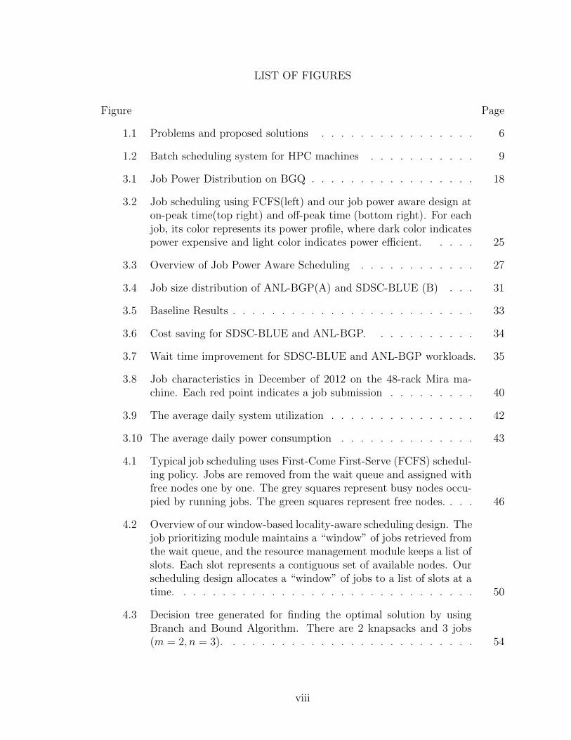
1.1 Problems and proposed solutions . . . . . . . . . . . . . . . . 6

1.2 Batch scheduling system for HPC machines . . . . . . . . . . . 9

3.1 Job Power Distribution on BGQ . . . . . . . . . . . . . . . . . 18

3.2 Job scheduling using FCFS(left) and our job power aware design aton-peak time(top right) and off-peak time (bottom right). For eachjob, its color represents its power profile, where dark color indicatespower expensive and light color indicates power efficient. . . . . 25

3.3 Overview of Job Power Aware Scheduling . . . . . . . . . . . . 27

3.4 Job size distribution of ANL-BGP(A) and SDSC-BLUE (B) . . . 31

3.5 Baseline Results . . . . . . . . . . . . . . . . . . . . . . . . . 33

3.6 Cost saving for SDSC-BLUE and ANL-BGP. . . . . . . . . . . 34

3.7 Wait time improvement for SDSC-BLUE and ANL-BGP workloads. 35

3.8 Job characteristics in December of 2012 on the 48-rack Mira ma-chine. Each red point indicates a job submission . . . . . . . . . 40

3.9 The average daily system utilization . . . . . . . . . . . . . . . 42

3.10 The average daily power consumption . . . . . . . . . . . . . . 43

4.1 Typical job scheduling uses First-Come First-Serve (FCFS) schedul-ing policy. Jobs are removed from the wait queue and assigned withfree nodes one by one. The grey squares represent busy nodes occu-pied by running jobs. The green squares represent free nodes. . . . 46

4.2 Overview of our window-based locality-aware scheduling design. Thejob prioritizing module maintains a “window” of jobs retrieved fromthe wait queue, and the resource management module keeps a list ofslots. Each slot represents a contiguous set of available nodes. Ourscheduling design allocates a “window” of jobs to a list of slots at atime. . . . . . . . . . . . . . . . . . . . . . . . . . . . . . . 50

4.3 Decision tree generated for finding the optimal solution by usingBranch and Bound Algorithm. There are 2 knapsacks and 3 jobs(m = 2, n = 3). . . . . . . . . . . . . . . . . . . . . . . . . . 54

viii

4.4 Scheduling result comparison between the default scheduler and ourdesign. The default scheduler (Subfigure A) makes job prioritizingsequence as 〈A,B,C,D〉, and the allocation for job A and B arefragmented, node 20 is left idle. Our design (Subfigure B) can makeoptimization so that every job gets a compact allocation and nonode is left idle. The prioritizing sequence obtained by our designis 〈C,A,B,E〉. . . . . . . . . . . . . . . . . . . . . . . . . . 58

4.5 Job size distribution of ANL-Intrepid and SDSC-BLUE . . . . . 60

5.1 Multiple jobs running concurrently with different allocations. Eachjob is represented by a specific color. a) shows the effect of con-tiguous allocation, which reduce the inter-job interference. b) showsnon-contiguous allocation, which may introduce both intra and inter-job interferences. . . . . . . . . . . . . . . . . . . . . . . . . 69

5.2 AMG communication matrix. The label of both the x and the yaxis is the index of MPI rank in AMG. The legend bar on the rightindicates the data transfer amount between ranks. . . . . . . . . 71

5.3 Crystal Router communication matrix. The label of both the x andthe y axis is the index of MPI rank in CrystalRouter. The legendbar on the right indicates the data transfer amount between ranks. 72

5.4 MultiGrid communication matrix. The label of both the x and they axis is the index of MPI rank in MultiGrid. The legend bar onthe right indicates the data transfer amount between ranks. . . . 73

5.5 Contiguous allocation in three different shapes. Red is a 3D balancedcube, green a 3D unbalanced cube, and blue a 2D mesh. . . . . . 76

5.6 Data transfer time of AMG, Crystal Router, and MultiGrid on 2Dmesh, 3D unbalanced, and 3D balanced allocation. . . . . . . . . 77

5.7 Data transfer time of AMG, Crystal Router, and MultiGrid on 3Dbalanced allocation using different mapping strategies. . . . . . . 78

5.8 Noncontiguous allocation. Each job is represented by a specificcolor. The nodes assigned to different jobs are interleaved; the sizesof allocation unit are 16, 8, and 2. . . . . . . . . . . . . . . . 79

5.9 Interjob interference study: “cont” indicates three applications run-ning side by side concurrently on the same network with contiguousallocation. To study the impact of noncontiguous allocation on inter-job interference, applications are run concurrently with interleavedallocations of different unit sizes, namely, 16 node, 8 node, and 2node. . . . . . . . . . . . . . . . . . . . . . . . . . . . . . . 80

ix

6.1 Five group slice of a 19-group dragonfly network. Job J1 is allocatedusing random placement, while Job J2 is allocated using contiguousplacement. . . . . . . . . . . . . . . . . . . . . . . . . . . . 89

6.2 Aggregate traffic and saturation time for Workload I under the con-figurations listed in Table 6.3. “CA” and “CPA” have equivalentbehavior. . . . . . . . . . . . . . . . . . . . . . . . . . . . . 95

6.3 Communication time distribution across application ranks in Work-load I. . . . . . . . . . . . . . . . . . . . . . . . . . . . . . 97

6.4 Aggregate workload traffic for routers serving specific applications.“CA” and “CPA” have equivalent behavior. More routers are in-volved in serving each application when random placement is in use,compared to contiguous placement. . . . . . . . . . . . . . . . 98

6.5 Aggregate traffic and saturation time for Workload II under theconfigurations listed in Table 6.3. . . . . . . . . . . . . . . . . 102

6.6 Communication time distribution across application ranks in Work-load II. The “bully”, sAMG, benefits from random placement andadaptive routing, while the “bullied”, MultiGrid and CrystalRouter,suffer performance degradation. . . . . . . . . . . . . . . . . . 102

6.7 Aggregate workload traffic for routers serving specific applications.More routers are involved in serving each application when randomplacement is in use, compared to contiguous placement. . . . . . 104

6.8 Application communication time. Workload I is running with allplacement and routing configurations. Methods prefixed with “H”represent the hybrid allocation approach. . . . . . . . . . . . . . 105

6.9 Application communication time. Workload I is running with threedifferent random placement policies coupled with three routing con-figurations. . . . . . . . . . . . . . . . . . . . . . . . . . . . 108

x

ABSTRACT

The batch scheduler is an important system software serving as the interface

between users and HPC systems. Users submit their jobs via batch scheduling portal

and the batch scheduler makes scheduling decision for each job based on its request

for system resources and system availability. Jobs submitted to HPC systems are

usually parallel applications and their lifecycle consists of multiple running phases,

such as computation, communication and input/output data. Thus, the running

of such parallel applications could involve various system resources, such as power,

network bandwidth, I/O bandwidth, storage, etc. And most of these system resources

are shared among concurrently running jobs. However, Today’s batch schedulers

do not take the contention and interference between jobs over these resources into

consideration for making scheduling decisions, which has been identified as one of the

major culprits for both the system and application performance variability.

In this work, we propose a cooperative batch scheduling framework for HPC

systems. The motivation of our work is to take important factors about jobs and the

system, such as job power, job communication characteristics and network topology,

for making orchestrated scheduling decisions to reduce the contention between con-

currently running jobs and to alleviate the performance variability. Our contributions

are the design and implementation of several coordinated scheduling models and algo-

rithms for addressing some chronic issues in HPC systems. The proposed models and

algorithms in this work have been evaluated by the means of simulation using work-

load traces and application communication traces collected from production HPC

systems. Preliminary experimental results show that our models and algorithms can

effectively improve the application and the system overall performance, HPC facilities’

operation cost, and alleviate the performance variability caused by job interference.

xi

1

CHAPTER 1

INTRODUCTION

1.1 Motivation

The high performance computing (HPC) systems comprise hundreds of thou-

sands compute nodes connected by large scale interconnected networks. The insa-

tiable demand for computing power from lots of scientific areas continues to drive the

involvement of ever-growing HPC systems. It is projected that by 2023, the exascale

HPC systems are expected to face many challenges[1]. Some of the most prominent

challenges are including, ever-increasing power consumption and energy cost, network

contention and job interference, concurrency and locality. These challenges demand

significant changes and great technical breakthroughs in many aspects of the current

HPC system software and hardware stack. In order to harness the great potential

of large scale HPC systems, lots of research studies have been focusing on bringing

solutions to these challenges from different layer of the system, such as new hardware

design, storage hierarchy, operating system and all kinds of system softwares.

The batch scheduler, serving as the interface between users and the HPC sys-

tems, is an integral part of the HPC system software stack. The users submit their

applications (jobs) via the batch scheduling portal and their jobs are scheduled and

dispatched by the batch scheduler to the HPC system for execution and return the

results to the users. Jobs submitted to HPC systems are usually parallel applications

and their lifecycle consists of multiple running phases, such as computation, commu-

nication and input/output data. Thus, the running of such parallel applications could

involve various system resources, such as power[2, 3], network bandwidth[4–7][8–11]

, I/O bandwidth[12, 13], storage[14][15], etc. And most of these system resources

are shared among concurrently running jobs. It has been identified that the con-

tention and interference among concurrently running jobs over the share resources

2

are the major culprits for both the system and application performance variability.

The motivation of this work is to explore possible batch scheduling algorithms and

methodologies to alleviate the performance variability introduced by job interference.

The traditional HPC system batch schedulers make scheduling decisions based

on the number of required nodes and expected run time of each job and they do

not take the contention and interference between jobs over these resources into con-

sideration. Making scheduling decisions without coordination could leads to severe

contention and interference among concurrently running jobs, which further cause

performance loss and variability. For example, when the batch scheduler allocates

computing nodes without any knowledge about jobs’ communication patterns, there

might be network contention between concurrently running jobs due to the overlapped

communication paths. The network contention introduces interference between those

jobs, thus causing severe performance degradation. We believe it is urgent to improve

today’s batch schedulers with a more orchestrated scheduling methodology. The de-

sign of such orchestrated batch scheduling framework requires deep understanding

about the problems that we target to solve. In this work, we provide in-depth study

about three major problems that the exascale HPC systems would possible to have.

1. Energy Cost. As HPC systems continue to grow, so does their energy con-

sumption. The cost spent on power consumption is now a leading component

of total cost of ownership(TCO) of HPC systems. The typical current petas-

cale system on average consumes 2-7 MW of power [16]. Case in point, the

Argonne Leadership Computing Facility (ALCF) budgets approximately $1M

annually for electricity to operate its primary supercomputer[2, 17]. Based on

current projections, exascale supercomputers will consume 60-130 MW, which

will prove to be an unbearable burden for any facility. Therefore, energy cost

savings are crucial for reducing the operational cost of exascale systems.

3

There is a significant number of research studies about improving energy ef-

ficiency for HPC systems and most of them focusing on the following top-

ics: energy-efficient or energy proportional hardware, dynamic voltage and fre-

quency scaling (DVFS) techniques, shutting down hardware components at low

system utilizations, power capping, and thermal management. Being orthogo-

nal to existing studies, our research focus on reducing the electricity bill of HPC

systems.

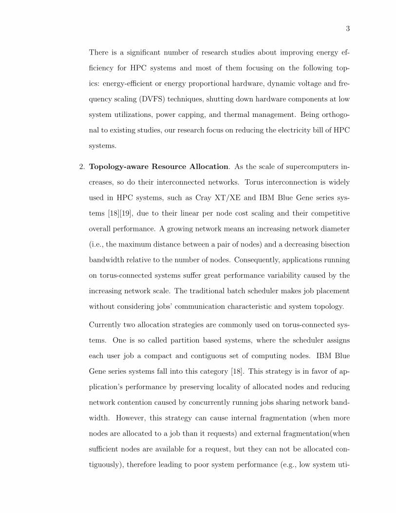
2. Topology-aware Resource Allocation. As the scale of supercomputers in-

creases, so do their interconnected networks. Torus interconnection is widely

used in HPC systems, such as Cray XT/XE and IBM Blue Gene series sys-

tems [18][19], due to their linear per node cost scaling and their competitive

overall performance. A growing network means an increasing network diameter

(i.e., the maximum distance between a pair of nodes) and a decreasing bisection

bandwidth relative to the number of nodes. Consequently, applications running

on torus-connected systems suffer great performance variability caused by the

increasing network scale. The traditional batch scheduler makes job placement

without considering jobs’ communication characteristic and system topology.

Currently two allocation strategies are commonly used on torus-connected sys-

tems. One is so called partition based systems, where the scheduler assigns

each user job a compact and contiguous set of computing nodes. IBM Blue

Gene series systems fall into this category [18]. This strategy is in favor of ap-

plication’s performance by preserving locality of allocated nodes and reducing

network contention caused by concurrently running jobs sharing network band-

width. However, this strategy can cause internal fragmentation (when more

nodes are allocated to a job than it requests) and external fragmentation(when

sufficient nodes are available for a request, but they can not be allocated con-

tiguously), therefore leading to poor system performance (e.g., low system uti-

4

lization and high job response time) [20]. The other is non-contiguous allocation

system, where free nodes are assigned to user job no matter whether they are

contiguous or not. Cray XT/XE series systems fall into this category [19]. Non-

contiguous allocation eliminates internal and external fragmentation as seen in

partition-based systems, thereby leading to high system utilization. Neverthe-

less, it introduces other problems such as scattering application processes all

over the system. The non-contiguous node allocation can make inter-process

communication less efficient and cause network contention among concurrently

running jobs [21], thereby resulting in poor job performance especially for those

communication-intensive jobs. Partition-based allocation achieves good job

performance by sacrificing system performance (e.g., poor system utilization),

whereas non-contiguous allocation can result in better system performance but

could severely degrade performance of user jobs (e.g, prolonged wait-time and

run-time). As systems continue growing in size, a fundamental problem arises:

how to effectively balance job performance with system performance on torus-

connected machines?

3. Network Contention and Job Interference. Supercomputers are usually

employed as a shared resource to accommodate many parallel applications (jobs)

running concurrently. These parallel jobs share the system infrastructure such

as network and I/O bandwidth, and inevitably there is contention over these

shared resources. As supercomputers continue to evolve, these shared resources

are increasingly the bottleneck for performance. Typically, multiple jobs are

running concurrently on the system, resulting in the shared use of resources,

particularly network links. A prominent problem with network sharing is the re-

sulting contention, which can cause communication variability and performance

degradation in affected jobs [4]. This performance degradation can propagate

into the queueing time of the following submitted jobs, thus leading to lower

5

system throughput and utilization [22].

On the widely used torus-connected HPC systems [23–25], two allocation strate-

gies are commonly used. The contiguous allocation strategy assigns to each job

a compact and contiguous set of computing nodes. The partition-based alloca-

tion approach used in Blue Gene series systems is an example of such a strategy

[26]. The contiguous strategy favors application performance through isolated

networking within a partition and the locality that implies. However, this strat-

egy can cause both internal fragmentation (when more nodes are allocated to

a job than it requests) and external fragmentation (when sufficient nodes are

available for a request, but they can not be allocated contiguously), therefore

leading to lower system utilization than is otherwise possible. On the other side

of the coin, the non-contiguous allocation strategy, used by the Cray XT/XE

series [27], assigns free nodes to jobs regardless of contiguity, though of course

efforts are made to maximize locality. While eliminating internal and external

fragmentation as seen in contiguous allocation systems, in return non-contiguous

allocations introduce network contention between jobs due to the interleaving

of job nodes. The non-contiguous placement policy can significantly reduce job

performance, especially for communication-intensive ones [4][9][28]. The net-

work contention between concurrently running jobs also exist on current HPC

systems with dragonfly networks[5][8]. How to intelligently make job place-

ment on exascale HPC systems to avoid network contention remains to be a

challenging problem.

1.2 Contributions

In this dissertation, we present a series of novel batch scheduling algorithms

and methodologies to solve the above identified problems. For each problem, we

have proposed a dedicated solution as shown in Figure 1.1. The contributions of this

6

dissertation are the design and implementation of each dedicated solution.

Computing Node

Network

Energy Cost

Fragmentation

Network

Contention

Job Interference

Energy Cost

Aware Scheduling

Locality Aware

Scheduling

Topology Aware

Scheduling &

Allocation

Origin of Problems Problems Solutions

Figure 1.1. Problems and proposed solutions

1. Energy Cost-aware Scheduling. There is a significant number of research

studies about improving energy efficiency for HPC systems and most of them

focusing on the following topics: energy-efficient or energy proportional hard-

ware, dynamic voltage and frequency scaling (DVFS) techniques, shutting down

hardware components at low system utilizations, power capping, and thermal

management. Being orthogonal to existing studies, we focus on reducing the

electricity bill of HPC systems via a smart job scheduling mechanism. The

rationale is based on a key observation of HPC jobs: parallel jobs have distinct

power consumption profiles [29][17]. We also notice that the dynamic electricity

pricing policies have been widely adopted in Europe, North America, Oceania,

and parts of Asia. For example, in the U.S.A, wholesale electricity prices vary

by as much as a factor of 10 from one hour to the next [30]. Under dynamic

pricing, the power grid has on-peak time (when it bears a heavier burden and

consequently the electricity price is higher) and off-peak time (when there is

7

less demand for electricity and the price is lower) alternatively in a day. The

novelty of our energy cost-aware scheduling mechanism is that it can reduce sys-

tem’s electricity bill by scheduling and dispatching jobs according to their power

profiles and the real time electricity price, while causing negligible impact on

the system’s utilization and scheduling fairness. Preferentially, it dispatches the

jobs with higher power consumption during the off-peak period, and the jobs

with lower power consumption during the on-peak period. We formalize this

scheduling problem into a standard 0-1 knapsack model, based on which we

apply dynamic programming to efficiently solve the scheduling problem. The

derived 0-1 knapsack model enables us to reduce energy cost during high elec-

tricity pricing period with no or limited impact to system utilization.

2. Locality-aware Scheduling.

The partition policy oriented schedulers achieve good job performance by sacri-

ficing system performance (e.g., poor system utilization), whereas non-partition

oriented schedulers can result in better system performance but could severely

degrade performance of user jobs (e.g, prolonged wait-time and run-time)[26][27].

We present a new scheduling design combining the merits of partition and non-

contiguous based scheduling for torus-connected machines. In this scheduling

mechanism, the batch scheduler takes a “window” of jobs (i.e., multiple jobs)

into consideration for making prioritizing and allocation decision, to prevent the

short-term decision from obfuscating future optimization. The job prioritizing

module maintains a “window” of jobs, and these jobs are placed into the win-

dow to maintain job fairness (e.g., through FCFS). Rather than allocating jobs

one by one from the head of the wait queue as existing schedulers do, we make

scheduling decision for a “window” of jobs at a time. The resource allocation

module takes a contiguous set of nodes as a slot and maintains a list of such

slots. These slots have different sizes and each may accommodate one or more

8

jobs. The allocation of the jobs in the window onto the slot list is conducted in

such a way as to maximize system utilization. We formalize the allocation of a

window of jobs to a list of slots as a 0-1 Multiple Knapsack Problem (MKP) and

present two algorithms, namely Branch&Bound and Greedy, to solve the MKP.

A series of trace-based simulations using job logs collected from production su-

percomputers indicate that this new scheduling design has real potentials and

can effectively balance job performance and system performance.

3. Topology-aware Scheduling&Allocation.

We envision that future HPC schedulers will adopt a flexible job scheduling

and allocation mechanism which combines the best of both contiguous and

non-contiguous allocation strategies. Such a flexible mechanism would take

shared resource needs of jobs into account when making allocation decisions

(e.g., network). With knowledge and analysis of job communication patterns, it

can be identified which jobs require network isolation and locality, and to what

degree. Then, rather than allocating each job in a “know-nothing” manner,

one may specialize allocation so that, for example, only the jobs with stringent

network needs are given compact, isolated allocations, resulting in maximized

utilization and minimized perceivable resource contention effects.

We provide an in-depth analysis of intra- and inter-job communication in-

terference with different job allocation strategies on both torus and dragon-

fly connected HPC systems. We selected three signature applications from

the DOE Design Forward Project [31] as examples to conduct detailed study

about their communication patterns. We use a sophisticated simulation toolkit

named CODES (standing for Co-Design of Multi-layer Exascale Storage Archi-

tectures) [32] as a research vehicle to evaluate the performance of these appli-

cations with various allocations in a controlled environment. We then analyze

9

the intra- and inter-job interference by simulating these applications running

exclusively and concurrently with different job placement policies. The insights

presented in this work can be very useful for the design of future HPC batch

job schedulers and resource managers.

Scheduling

Module

Resource

Management

Logging Module

Queuing Module

Cooperative Batch Scheduling Framework

HPC System

Scheduled Jobs

System Status

System LogsHistorical data

Queue Status

Scheduling Decision

Users

Figure 1.2. Batch scheduling system for HPC machines

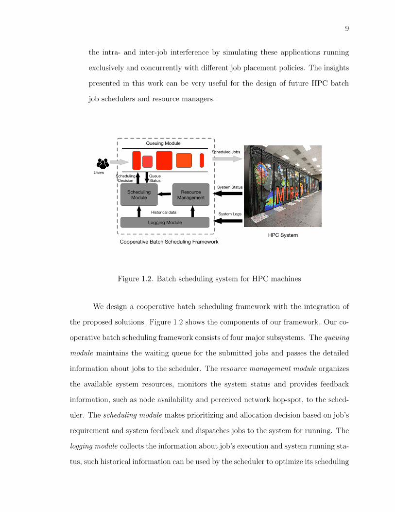
We design a cooperative batch scheduling framework with the integration of

the proposed solutions. Figure 1.2 shows the components of our framework. Our co-

operative batch scheduling framework consists of four major subsystems. The queuing

module maintains the waiting queue for the submitted jobs and passes the detailed

information about jobs to the scheduler. The resource management module organizes

the available system resources, monitors the system status and provides feedback

information, such as node availability and perceived network hop-spot, to the sched-

uler. The scheduling module makes prioritizing and allocation decision based on job’s

requirement and system feedback and dispatches jobs to the system for running. The

logging module collects the information about job’s execution and system running sta-

tus, such historical information can be used by the scheduler to optimize its scheduling

10

decisions for the future workloads. The logging module is also responsible for off-line

log analysis. Our cooperative batch scheduling framework is equipped with different

scheduling policies that are designated for scheduling jobs and allocating resources in

an coordinated way. Thus, our batch scheduling framework is capable of making or-

chestrated scheduling decisions with regard to the contention and interference among

concurrently running jobs over the shared resources, and will significantly improves

the system performance while reducing performance variability.

The contributions in this dissertation have led to 12 peer reviewed publications,

and two publications that are under review.

• Xu Yang, Zhou Zhou, Sean Wallace, Zhiling Lan, Wei Tang, Susan Coghlan,

Michael E Papka, Integrating Dynamic Pricing of Electricity into Energy Aware

Scheduling for HPC Systems, Proc. of SC’13, 2013.

• Xu Yang, John Jenkins, Misbah Mubarak, Robert B Ross, Zhiling Lan, Watch

Out for the Bully! Job Interference Study on Dragonfly Network, Proc of SC16,

2016.

• Xu Yang, John Jenkins, Misbah Mubarak, Xin Wang, Robert B Ross, Zhiling

Lan, Study of intra-and interjob interference on torus networks, Parallel and

Distributed Systems (ICPADS), 2016 IEEE 22nd International Conference on.

• Xu Yang, Zhou Zhou, Wei Tang, Xingwu Zheng, Jia Wang, Zhiling Lan, Bal-

ancing Job Performance with System Performance via Locality-Aware Schedul-

ing on Torus-Connected Systems, Proc. of Cluster Computing (CLUSTER),

2014 IEEE International Conference on.

• Sean Wallace, Xu Yang, Venkatram Vishwanath, William E Allcock, Susan

Coghlan, Michael E Papka, Zhiling Lan, A Data Driven Scheduling Approach

for Power Management on HPC Systems, Proc of SC16, 2016.

11

• Zhou Zhou, Xu Yang, Zhiling Lan, Paul Rich, Wei Tang, Vitali Morozov,

Narayan Desai, Improving Batch Scheduling on Blue Gene/Q by Relaxing 5D

Torus Network Allocation Constraints, Proc. of IPDPS’15, 2015.

• Zhou Zhou, Xu Yang, Dongfang Zhao, Paul Rich, Wei Tang, Jia Wang, Zhiling

Lan, I/O-Aware Batch Scheduling for Petascale Computing Systems, Proc. of

Cluster Computing (CLUSTER), 2015 IEEE International Conference on

• Zhou Zhou, Xu Yang, Zhiling Lan, Paul Rich, Wei Tang, Vitali Morozov,

Narayan Desai, Improving Batch Scheduling on Blue Gene/Q by Relaxing 5D

Torus Network Allocation Constraints, accepted by IEEE Trans. on Parallel

and Distributed Systems (TPDS), 2016.

• Zhou Zhou, Xu Yang, Dongfang Zhao, Paul Rich, Wei Tang, Jia Wang,

Zhiling Lan, I/O-Aware Bandwidth Allocation for Petascale Computing Sys-

tems,Journal of Parallel COmputing (ParCo), 2016.

• Dongfang Zhao, Xu Yang, Iman Sadooghi, Gabriele Garzoglio, Steven Timm,

Ioan Raicu, High-performance storage support for scientific applications on the

cloud, Proc of the 6th Workshop on Scientific Cloud Computing.

• Xingwu Zheng, Zhou Zhou, Xu Yang, Zhiling Lan, Jia Wang, Exploring Plan-

Based Scheduling for Large-Scale Computing Systems, Proc. of Cluster Com-

puting (CLUSTER), 2016 IEEE International Conference on.

• Jiaqi Yan, Xu Yang, Dong Jin, Zhiling Lan, Cerberus: A Three-Phase Burst-

Buffer-Aware Batch Scheduler for High Performance Computing, Proc. of SC’16,

Technical Program Posters.

1.3 Outline

12

The rest of this dissertation is organized as follows. Chapter 2 gives knowledge

about High Performance Computing and supercomputers, batch schedulers, workload

traces, application communication traces and the simulation tools used in our work.

Chapter 3 presents our work about reducing energy cost for HPC systems. Chapter

4 presents topology-aware scheduling for torus connected HPC systems. Chapter 5

presents the in-depth analyses about intra and interjob interference on torus network.

Chapter 6 presents our study about network contention and job interference on drag-

onfly network. Chapter 7 concludes the dissertation by summarizing the contributions

and discussing some future work on extending the current scheduling framework.

13

CHAPTER 2

BACKGROUND

2.1 HPC Systems

The target platform in this dissertation is the high performance computing

(HPC) system which usually referred as supercomputer. Today’s supercomputers

consist of hundreds of thousands compute nodes connected by high bandwidth inter-

connected network. We introduce two HPC systems with different network topologies.

Our work are based on the abstracted model of both network topologies.

As the scale of supercomputers increases, so do their interconnected networks.

Torus interconnection is widely used in HPC systems, such as Cray XT/XE and IBM

Blue Gene series systems [18][19], due to their linear per node cost scaling and their

competitive overall performance. Mira[33], a 10 PFLOPS (peak) Blue Gene/Q system

in Argonne National Laboratory, is a Torus connected HPC system. The computing

nodes in Mira are grouped into midplanes, each midplane contains 512 nodes in a

4× 4× 4× 4× 2 sub-torus/mesh structure. Mira has 48 racks arranged in three rows

of sixteen racks. Each rack has two such midplanes, which contains 1024 sixteen-core

nodes, for a total of 16384 cores per rack, giving a total of 786432 cores. Mira was

ranked fifth in the latest Top500 list[34].

The high-radix, low-diameter dragonfly topology can lower the overall cost of

the interconnect, improve network bandwidth and reduce packet latency [35], making

it a very promising choice for building supercomputers with millions of cores. The

dragonfly is a two-level hierarchical topology, consisting of several groups connected

by all-to-all links. Each group consists of a routers connected via all-to-all local chan-

nels. For each router, p compute nodes are attached to it via terminal links, while h

links are used as global channels for intergroup connections. The resulting radix of

14

each router is k = a + h + p− 1. Different computing centers could choose different

values for a, h, p when deploying their dragonfly network. The adoption of proper a,

h, p involves many factors such as system scale, building cost and workload character-

istics. One implementation of the dragonfly topology is Cori, a Cray Cascade system

(Cray XC30)[36] deployed at NERSC, Lawrence Berkeley National Laboratory. The

building block of Cori is an Aries router with four terminal ports and 30 network

ports. Each router has four compute nodes attached through terminal ports. Sixteen

routers form a chassis and six chassis are put into the same group. Each router has

20 ports for local channels, that is 15 ports to connect all the other routers in the

same chassis and 5 more ports to connect routers from other chassis. Each router has

10 ports for global channels for the connection between other groups.

2.2 Batch Scheduler

There are a number of source management and job scheduling tools dedicated

to HPC systems. Some of the commonly used by computing facilities are includ-

ing Moab [37] from Adaptive computing, PBS [38] from Altair, SLURM [39] from

SchedMD and Cobalt [40] from Argonne National Laboratory. Tools like Moab, PBS

are commercial products and SLURM and Cobalt are open source projects.

We have developed a simulator named CQSim to evaluate our design at scale.

The simulator is written in Python, and is formed by several modules such as job

module, node module, scheduling policy module, etc. Each module is implemented

as a class. The design principles are reusability, extensibility, and efficiency. The

simulator takes job events from the trace, and an event could be job submission, start,

end, and other events. Based on these events, the simulator emulates job submission,

allocation, and execution based on specific scheduling and allocation policies. CQsim

is open source, and is available to the community[41].

15

2.3 Workload Trace

The HPC system can accommodate multiple users to run their jobs simul-

taneously. The system records all kinds of events regarding to each job, such as

its submission, entering the waiting queue, start running, failure and completion in

chronological order. The collection of all these events recorded by the system produces

is referred as workload traces. In such workload trace file, each record is basically

composed of timestamp, event type, executable filename, job size, location, wait time,

running time, etc. The workload traces used in our study are archived on the Parallel

Workloads Archive[42].

2.4 Application Communication Trace

A parallel application usually conforms to a combination of several basic com-

munication patterns [43]. At its different execution phases, the application’s commu-

nication behavior may follow different basic patterns respectively. There are many

profiling tools available to capture information regarding communication patterns of

parallel applications [44–48]. In this work, we select three representative applications

from the DOE Design Forward Project. Each application exhibits a distinctive com-

munication pattern that is commonly seen in HPC applications. We believe that the

communication patterns of these applications are representative of a wide array of

applications running on leadership-class machines. Specifically, we study the Alge-

braic MultiGrid Solver (AMG), Geometric MultiGrid (MultiGrid) and CrystalRouter

MiniApps. For each application, we collect its communication trace generated by SST

DUMPI[47]. The detail about the DUMPI traces and communication pattern of these

applications will be introduced in later section.

2.5 Simulation Tool

A simulation toolkit named CODES enables the exploration of simulating dif-

16

ferent HPC networks with high fidelity [32][49]. CODES is built on top of Rensselaer

Optimistic Simulation System (ROSS) parallel discrete-event simulator, which is ca-

pable of processing billions of events per second on leadership-class supercomputers

[50]. CODES support both torus and dragonfly network with high fidelity flit-level

simulation. CODES has this network workload component that is capable of con-

ducting trace-driven simulations. It can take real MPI application traces generated

by SST DUMPI [47] to drive CODES network models.

17

CHAPTER 3

ENERGY COST AWARE SCHEDULING DRIVEN BYDYNAMIC PRICING ELECTRICITY

3.1 Overview

The research literature to date mainly aimed at reducing energy consumption

in HPC environments. Being orthogonal to existing studies we propose a job power

aware scheduling mechanism to reduce HPC’s electricity bill without degrading the

system utilization. The rationale is based on a key observation of HPC jobs: parallel

jobs have distinct power consumption profiles. In our recent work [3], we provided

analysis of a one-month workload on Mira, the 48-rack IBM Blue Gene/Q (BGQ)

system at Argonne National Laboratory (Figure 3.1). The histogram displays per-

centages partitioned by size ranging from single rack jobs to full system runs. The

power consumption of those jobs varies from around 40 kW/rack to 90 kW/rack.

We hypothesize that it is possible to save a significant amount on an electric

bill by exploiting a dynamic electricity pricing policy. To date, dynamic electricity

pricing policies have been widely adopted in Europe, North America, Oceania, and

parts of Asia. For example, in the U.S.A, wholesale electricity prices vary by as much

as a factor of 10 from one hour to the next [30]. Under dynamic pricing, the power

grid has on-peak time (when it bears a heavier burden and consequently the electricity

price is higher) and off-peak time (when there is less demand for electricity and the

price is lower) alternatively in a day.

In this work, we develop a job power aware scheduling mechanism. The novelty

of this scheduling mechanism is that it can reduce system’s electricity bill by schedul-

ing and dispatching jobs according to their power profiles and the real time electricity

price, while causing negligible impact on the system’s utilization and scheduling fair-

ness. Preferentially, it dispatches the jobs with higher power consumption during

18

Figure 3.1. Job Power Distribution on BGQ

19

the off-peak period, and the jobs with lower power consumption during the on-peak

period.

A key challenge in HPC scheduling is that system utilization should not be

impacted. HPC systems require a tremendous capital investment, hence taking full

advantage of this expensive resources is of great importance to HPC centers. Unlike

the utilization of Internet data centers, which only fluctuate about 20%, systems at

HPC centers are highly employed with a typical utilization around 50%-80% [42]. To

address this challenge, we propose a novel window-based scheduling mechanism[51].

In this work, rather than allocating jobs one by one from the front of the wait queue as

existing schedulers do, we schedule and dispatch a ”window” of jobs at a time. Those

jobs placed into the window are chosen to maintain job fairness, and the allocation

of these jobs onto system resources is done in such a way as to minimize electricity

bill. Two scheduling algorithms, namely a Greedy policy and a 0-1 Knapsack based

policy, are presented in this work for decision-making.

We evaluate our job power aware scheduling design via extensive trace-based

simulations and a case study of Mira. In this paper, we present a series of experiments

comparing our design against the popular first-come, first-serve (FCFS) scheduling

policy, with backfilling done in three different aspects (electricity bill saving, schedul-

ing performance, and job performance). Our preliminary results demonstrate that

our design can cut electricity bill by up to 23% without an impact on overall system

utilization. Considering HPC centers often spend millions of dollars on even the least

expensive energy contracts, such savings can translate into a reduction of hundreds

of thousands in terms of TCO.

The structure of this chapter is as follows. In section 3.2, we discuss the

existing work about energy reduction for HPC systems. Section 3.3 describes the job

power aware scheduling problem. Section 3.4 gives a detailed description of our job

20

power aware scheduling design. Sections 3.5-3.7 present our evaluation methodology,

trace-based simulations, and a case study by comparing our design against the widely-

used FCFS scheduling policy under a variety of configurations. Our findings are

presented in Section 6.9.

3.2 Related Work

First, we give a brief survey of dynamic electricity pricing policies in different

countries to demonstrate the applicability of this work. The European Exchange

Market (EEX) in Germany, PowerNext in France, and APX in the Netherlands and

Iberian market all vary their cost of electricity on an hourly basis [52]. In [53], the

author stated dynamic electricity pricing policies are well adopted in Nordic countries

as Norway, Finland, Sweden, and Denmark. Other power markets such as England,

New Zealand, and Australia also have similar policies. Since the electricity crisis

in 2011-2012, the Japanese Ministry of Economy, Trade and Industry (METI) has

initiated the Smart Community Pilot Projects in four cities in Japan(Yokohama,

Toyota, Kyoto, and Kitakyushu) to investigate the effect of dynamic pricing and

smart energy equipment on residential electricity demand [54]. In China, major cities

such as Beijing, Shanghai, Guangzhou have initiated dynamic electricity pricing for

both domestic and industrial use since 2006. Dynamic electricity pricing has also

been carried out in several provinces such as Zhejiang, Jiangsu, and Guangdong.

As we can see from the survey above, the dynamic electricity pricing policy

has already been carried out in power markets in Europe, North America, Oceania,

and China. Japan has initiated preliminary tests in some major cities to see the effect

of this dynamic electricity pricing policy on the reduction of electricity consumption.

While in this study we evaluate our design based on the on-/off-peak electricity pricing

in U.S.A, we believe our design is applicable to other countries(e.g., those listed above)

for cutting the electricity bill of their HPC systems.

21

Although there is no known effort to provide job power aware scheduling sup-

port in the field of HPC, there is a large body of related work. Due to space lim-

itations, in this section we discuss some closely related studies and point out key

differences among them.

From the hardware perspective, hardware vendors are dedicated to produce

energy-efficient devices. For instance, Barroso and Holzle argued that the power

consumption of a machine should be proportional to its workload, i.e., it should

consume no power in idle state, almost no power when the workload is very low,

and eventually more power when the workload is increased [55]. Ideally, an energy

proportional system could save half of the energy used in data center operations. Li

et al. optimized the power/ground grid to make the power supply more efficient for

the chip [56].

Since processor power consumption is a significant portion of the total sys-

tem power (roughly 50% under load [57]), DVFS is widely used for controlling CPU

power [58]. By running a processor at a lower frequency/voltage, energy savings can

be achieved at the expense of increased job execution time. In order to meet user’s

SLAs (Service Level Agreements), DVFS is typically applied at the period of low

system activity. Some research studies on this topic can be found in [59] [60] [61] [62].

In a typical HPC system, nodes often consume considerable energy in idle state

without any running application. For example, an idle Blue Gene/P rack still has a

DC power consumption of about 13 kW [29]. During low system utilization, some

nodes or their components could be shut down or switched to a low-power state.

This strategy tries to minimize the number of active nodes of a system while still

satisfying incoming application requests. Since this approach is highly dependent on

system workload, the challenge is to determine when to shut down components and

how to provide a suitable job slowdown value based on the availability of nodes.

22

Hikita et al. [57] performed an empirical study by implementing an energy-

aware scheduler for an HPC system. The operation of the scheduler is simple: if

a node is inactive for 30 minutes, it is powered off; when the node is required for

job execution, it is powered on and moved to an active state. Powering up a node

on their system takes approximately 45 minutes, which is substantial. This strategy

can improve power efficiency by 39% at best. Because the rebooting of a node may

consume significant time that will lead to a performance degradation if it happens to

be peak job request period and more nodes are required than the active ones.

Pinheiro et al. [59] presented a mechanism that dynamically turns cluster nodes

on and off. This approach uses load consolidation to transfer workload onto fewer

nodes so that idle nodes can be turned off. The experimental tests on a static 8-node

cluster indicate a 19% saving in energy. It takes about 100 seconds to power on a

server and 45 seconds to shut it down on the cluster. The degradation in performance

is approximately 20%.

Thermal management techniques are another method frequently discussed in

the literature [60][62]. The rationale is that higher temperatures have a large impact

on system reliability and can also increase cooling costs. By using thermal manage-

ment, system workload is adjusted according to a predefined temperature threshold:

if the temperature on a server rises above that threshold, its workload is reduced.

Disadvantages of thermal management are delayed response, high risk of overheating,

excessive cooling and recursive cycling [62].

Many data centers use power capping or power budgeting to reduce the total

power consumption. The operator can set a threshold of power consumption to

ensure the actual power of the data center does not exceed it [63]. It prevents sudden

rises in power supply and keeps the total power consumption under a predefined

budget. Basically, the power consumption can be reduced by rescheduling tasks

23

or CPU throttling, for example, Etinski et al. proposed a parallel job scheduling

policy based on integer linear programming under a given power profile [61]. Lefurgy

et al. presented a technique for high density servers that controls the peak power

consumption by implementing a feedback controller [64].

This work has two major differences as compared to our previous work [65].

First, our previous work targets Blue Gene/P systems, which have a special require-

ment on job scheduling, i.e., available nodes must be connected in a job specific

shape before they can be allocated to a job [51][66]. This work intends to provide

a generic job power aware scheduling mechanism for various HPC systems. Second,

our previous work relies on a power budget (similar to power capping) for energy cost

saving, which degrades system utilization slightly during on-peak electricity price pe-

riod. The scheduling policies presented in this work do not use power budget, and

they minimize the electricity bill without impacting system utilization, during both

on-peak and off-peak electricity pricing periods.

3.3 Problem Description

Typically, user jobs are submitted to an HPC system through a batch sched-

uler, and then wait in a queue for the requested amount of system resources to become

available. There may be one or multiple job queues with different priories. A job is

generally defined by its arrival time, its estimated runtime, the amount of computing

nodes requested, etc. The scheduler is responsible for assigning computing nodes to

the jobs in the queues. FCFS with backfilling is a commonly used scheduling policy

in HPC [67]. Under this policy, the scheduler picks a job from the head of the wait

queue and dispatches it to the available system resources. The nodes assigned to a

job become unavailable until the job is complete (i.e., space sharing).

As mentioned in Section 3.1, our work is based on two key observations in

24

HPC: (1) electricity price is dynamically changing within a day; and (2) HPC jobs

have distinct power consumption profiles. We shall point out that usually HPC jobs

also tend to be repetitive. These repetitive jobs can be easily identified by user ID,

project, expected runtime, etc. A batch scheduler can extract job power profile based

on historical data and use it for power aware scheduling. For the simplicity of method

description, we assume that a daily electricity price is divided into on-peak and off-

peak periods, where on-peak period is referred to the time when more electricity is

demanded (e.g., during the daytime). By exploring these two observations, the basic

idea of our work is to allocate jobs with lower power consumption profiles during

on-peak time and to allocate jobs with higher power consumption profiles during off-

peak time. Furthermore, the allocation is made under the assumption that there will

be no impact to system utilization, meaning that a situation where a job is waiting

in the queue while there is a sufficient amount of idle/available computing nodes is

not allowed.

Getting job power consumption profiles is feasible on today’s supercomputers.

Most production HPC systems are deployed with built-in sensors that monitor the

health status of its hardware components. These sensors, deployed in various locations

inside the system, report environmental conditions such as motherboard, CPU, GPU,

hard disk and other peripherals for temperature, voltage, and/or fan speed. A number

of software tools/interfaces are publicly available for users to access these sensor

readings [68][18][19][3].

Figure 3.2 pictorially illustrates an example to highlight the key idea of our

design as compared to the conventional FCFS. Suppose five jobs J0, J1, J2, J3, J4 are

submitted to a 12-node system. Each job is associated with several parameters, such

as the amount of nodes needed, the estimated runtime, etc. Further, each job is

also associated with a power consumption profile pi, which can be determined from

25

historical data [3]. Suppose these jobs have the following parameters:

Job Power Profile (W/node) Job Size

J0 50 6

J1 20 3

J2 40 3

J3 30 3

J4 10 6

Under the conventional FCFS policy, the scheduling sequence is always <

J0, J1, J2 > in spite of the scheduling time. Our scheduling mechanism provides

different scheduling sequences depending on the dynamic electricity price and job’s

power profile. More specifically, our scheduling algorithm allocates < J4, J1, J3 >

during the on-peak period, and allocates < J0, J2, J3 > during the off-peak period.

By comparing the total power consumptions of using FCFS to that of our design, it

is clear that our design is able to reduce the accumulated power consumption during

the on-peak time where as to increase the accumulated power consumption during

the off-peak time, hence reducing the overall electricity bill.

Figure 3.2. Job scheduling using FCFS(left) and our job power aware design at on-peak time(top right) and off-peak time (bottom right). For each job, its colorrepresents its power profile, where dark color indicates power expensive and lightcolor indicates power efficient.

26

Table 3.1. Nomenclature

Symbol Description

ni job size, i.e., the number of nodes that are requested by Job i

pi the average power consumption per node.

Nt the amount of available nodes in the system at time t.

N system size, i.e., the number of nodes in the system.

T the time span from the start of the first job to the end of the last job.

w scheduling window size, i.e., the number of jobs in the window .

3.4 Methodology

In Table 3.1, we list the nomenclature that will be used in the rest of this

paper. Figure 3.3 gives an overview of our job power aware scheduling design. Our

design contains two key techniques. One is the use of a scheduling window to take

into consideration job features such as job fairness, and the other is the scheduling

policy to balance energy usage and scheduling performance.

3.4.1 Scheduling Window. Balancing fairness and system performance is always

a big concern for a scheduling algorithm. The simplest way to ensure fairness and

high system performance is to use a strict FCFS policy combined with backfilling,

where jobs are started in the order of their arrivals [67].

In this work, rather than allocating jobs one by one from the front of the

wait queue, we propose a novel window-based scheduling mechanism that allocates a

window of jobs. The selection of jobs into the window is based on certain user-centric

metrics, such as job fairness while the allocation of these jobs onto system resources

is determined by certain system-centric metrics such as system utilization and energy

consumption. By doing so, we are able to balance different metrics, representing both

user satisfaction and system performance.

27

Figure 3.3. Overview of Job Power Aware Scheduling

Given that FCFS is commonly used by production batch schedulers in HPC,

we now describe how our window based scheduling works with FCFS. We maintain

a scheduling window in front of the job queue, and the submitted jobs enter the job

queue first and then into the scheduling window. The selection of jobs is based on

job arrival times, thereby guaranteeing job fairness; the allocation of the jobs from

the window to the available system nodes is based on job power profiles, which will

be described later.

Typically, the window size should be determined based on system workload

such that a large window is preferred in case of high workload. For typical workloads

at production supercomputers, we find that a window size from 10 to 30 jobs can

28

achieve reasonable electricity bill savings.

3.4.2 Job Power Aware Scheduling Policies. In this work, we develop two

power aware scheduling policies. The first is a Greedy policy, where jobs are allocated

entirely based on the values of their power profiles. The second is a 0-1 Knapsack

based policy, where both job power profile and system utilization are taken into

consideration during decision making.

Greedy Policy. In the Greedy Policy, all the jobs in the scheduling window are

first sorted by their power profiles. During the on-peak electricity price period,

all the jobs in the scheduling window are sorted in a decreasing order based on

their power profiles; conversely, they are sorted in an increasing order during

the off-peak period. After the sorting, the scheduler will dispatches the ordered

jobs out of the scheduling window. Greedy policy is simple and fast. Suppose

the number of jobs in the window size is n, then the complexity of the algorithm

is O(nlgn).

O-1 Knapsack based Policy. In the 0-1 Knapsack policy, the only difference be-

tween on-peak and off-peak scheduling selection is the aggregated power con-

sumption: during the on-peak period, the goal is to minimize the value; during

the off-peak period, the goal is to maximize the value. In the following, we

present the 0-1 Knapsack based policy works at off-peak time.

Suppose there are Nt available nodes in the system, the scheduling window

size is w {Ji, |1 6 i 6 w}, and each job Ji requires ni nodes, with a power profile of

pi. Now, the scheduling problem can be formalized as follows:

Problem 1. To selecting a subset of {Ji, |1 6 i 6 k} from the scheduling win-

dow such that the aggregate nodes∑

1≤i≤k ni is no more than Nt, with the objective

of maximizing the aggregated power consumption∑

1≤i≤k ni · pi.

29

The above problem can be formalized into a 0-1 Knapsack problem. We set

the available nodes Nt as the knapsack’s size and consider the jobs in the scheduling

window as the objects that we intend to put into the knapsack. For each job, its

power profile (measured in W/node or kW/rack) is its value, the number of required

node is considered as the weight. Hence we can further transform Problem 1 into a

standard 0-1 Knapsack model.

Problem 2. To determine a binary vector

X = {xi, |1 6 i 6 k} such that:

maximize∑1≤i≤k

xi · pi, xi = 0 or 1

subject to∑1≤i≤k

xi · ni ≤ Nt

(3.1)

The standard 0-1 Knapsack model can be solved in pseudo-polynomial time

by using dynamic programming [69]. To avoid redundant computation, when imple-

menting this algorithm we use the tabular approach by defining a 2D table G, where

G[k, w] denotes the maximum gain value that can be achieved by scheduling jobs

{ji|1 ≤ i ≤ k} which require no more than Nt computing nodes, where 1 ≤ k ≤ J .

G[k, w] has the following recursive feature:

G[k,w]=

0 kw = 0

G[k−1,w] wi ≥ w

max(G[k−1,w],vi+G[k−1,w−wi]) wi ≤ w

(3.2)

The solution G[J,Nt] and its corresponding binary vector X determine the

selection of jobs scheduled to run. The computation complexity of Equation 3.2 is

30

O(J ·Nt).

During on-peak time, 0-1 Knapsack-based policy is modified by changing the

selection criterion into minimizing the total value of the objects in the knapsack with

the constraint of knapsack size.

3.5 Evaluation Methodology

We conduct a series of experiments using trace-based simulations. In our

experiments, we compare our design as against the well-known FCFS scheduling

policy [67]. In the rest of the paper, we simply use Greedy, Knapsack, and FCFS

to denote our scheduling policies and the conventional batch scheduling policy. This

section describes our evaluation methodology, and the experimental results will be

presented in the next section.

3.5.1 CQSim: Trace-based Scheduling Simulator. Simulation is an integral

part of our evaluation of various scheduling policies as well as their aggregate effect on

performance and power consumption. We have developed a simulator named CQSim

to evaluate our design at scale. The simulator is written in Python, and is formed

by several modules such as job module, node module, scheduling policy module,

etc. Each module is implemented as a class. The design principles are reusability,

extensibility, and efficiency. The simulator takes job events from a trace, and an event

may be job submission, job start, job end, and other events. Based on these events,

the simulator emulates job submission, allocation, and execution based on specific

scheduling policy. CQsim is open source, and is available to the community [41].

3.5.2 Job Traces. In this work, we use two real workload traces collected from

production supercomputers to evaluate our design. The objective of using multiple

traces is to quantify the impact of different factors on electricity bill saving. The first

trace we used is from a machine named Blue Horizon at the San Diego Supercomputer

31

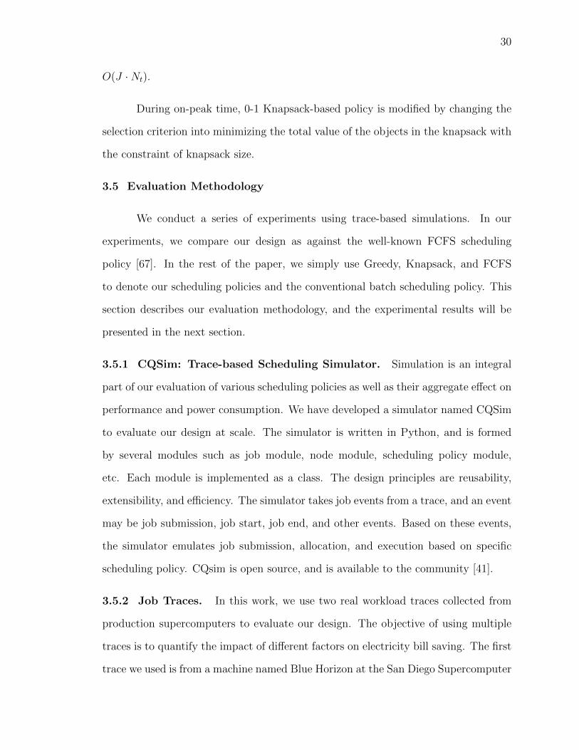
Center (denoted as SDSC-BLUE in the paper), which ran 14,4830 jobs in 2001.

Figure 3.4. Job size distribution of ANL-BGP(A) and SDSC-BLUE (B)

The second trace we used is from two racks of the IBM Blue Gene/P machine

named Intrepid at Argonne (denoted as ANL-BGP in the paper) [70][71]. This trace

contains 26,012 jobs. Since this trace is extracted out of the original 40-rack workload,

the utilization rate is relatively low. A well-known approach to remedy this problem

is to decrease job arrival intervals by a certain rate [72]. After we decrease job arrival

intervals by 40%, the trace becomes 5-month long with the utilization rate ranging

between 39% and 88%. Figure 4.5 summarize job size distribution of these traces.

ANL-BGP is used to represent capability computing where the computing power is

explored to solve larger problems, whereas SDSC-BLUE is used to represent capacity

computing where the computing power is utilized to solve a large number of small

problems.

3.5.3 Dynamic Electricity Price. In our experiments, we set two different

electricity prices: on-peak and off-peak pricing. We set the price in on-peak time

(from 12pm to 12am) higher than the off-peak time (from 12am until 12pm). This is

done to simplify our calculation and statistical analysis. Indeed, we are not concerned

about the absolute value of electricity price; instead the ratio of on-peak price to off-

peak price is more important. According to [30], the most common ratio of on-peak

32

and off-peak pricing varies from 1:2 to 1:5. Hence we set the default ratio to 1:3.

3.5.4 Job Power Profile. Since job power profile is not included in the original

traces, we assign each job with a power profile between 20 to 60W per node using a

normal distribution according to the power profile presented in Figure 3.1. Similarly,

we are not concerned about the absolute power profile value; instead the ratio of

maximum power profile to minimal power profile is more important. The default

ratio is set to 1:3.

3.5.5 Evaluation Metrics. In this work, we use three metrics to evaluate our

design against the conventional FCFS.

Electricity Bill Saving. We calculate the relative difference between the electricity

bill using our design and FCFS to measure the electricity bill savings achieved

by our design. The simulator sums up electricity bill on a daily basis for the

calculation of this metric.

System Utilization Rate. This metric denotes the ratio of the node-hours that are

used for useful computation to the elapsed system node-hours. Specifically, let

T be the total elapsed time for J jobs, ci be the completion time for job i and

si be its the start time, and ni be the size of job i, then system utilization rate

is calculated as ∑0≤i≤J (ci − si) · ni

N · T(3.3)

Average Job Wait Time. For each job, its wait time refers to the time elapsed

between the moment it is submitted to the moment it is allocated to run. This

metric is calculated as the average across all the jobs submitted to the system.

This metric is a user-centric metric, measuring scheduling performance from

user’s perspective.

33

3.6 Experiment Results

We conduct four sets of experiments on the traces described in Section 4.5.2

to evaluate our design as against FCFS.

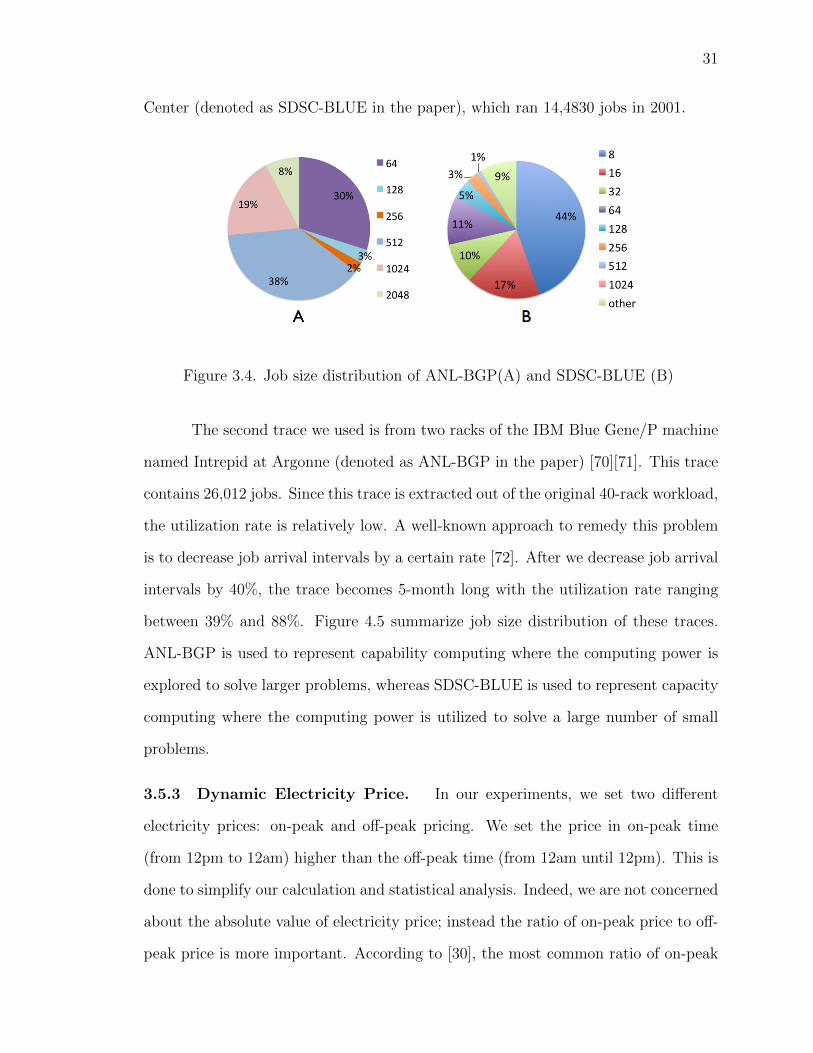
3.6.1 Baseline Results. Baseline results are presented in Figures 3.5(a) - 3.7(b),

where we use the default setting described in Sections 3.5.3-3.5.4, meaning that job

power profile ratio is 1:3 and the off-peak/on-peak pricing ratio is 1:3. On production

supercomputers, the scheduling frequency is typically on the order of 10 to 30 seconds.

Hence, the simulator is set to make a scheduling decision every 10 seconds.

Since our evaluation focuses on the relative reduction of electricity bills, so the

absolute value of idle power consumption, which is set to 0 in our experiments, does

not impact the results.

(a) System Utilization of SDSC-BLUE (b) System Utilization of ANL-BGP

Figure 3.5. Baseline Results

Figure 3.5(a) and Figure 3.5(b) compare system utilization rates achieved by

using different job scheduling policies. It is clear that the utilization degradation

introduced by our design is always less than 5%, no matter which scheduling policy we

choose (Greedy or Knapsack). Moreover, for the 3rd and 5th month of SDSC-BLUE

trace, both our scheduling policies may achieve higher system utilization compared to

34

FCFS. These results clearly demonstrate that our scheduling design brings negligible

impact on system utilization, which is critical to HPC systems.

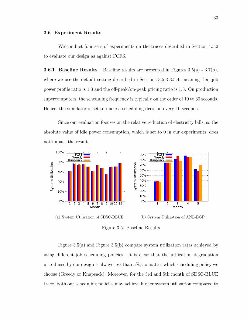
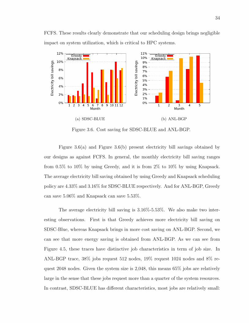
(a) SDSC-BLUE (b) ANL-BGP

Figure 3.6. Cost saving for SDSC-BLUE and ANL-BGP.

Figure 3.6(a) and Figure 3.6(b) present electricity bill savings obtained by

our designs as against FCFS. In general, the monthly electricity bill saving ranges

from 0.5% to 10% by using Greedy, and it is from 2% to 10% by using Knapsack.

The average electricity bill saving obtained by using Greedy and Knapsack scheduling

policy are 4.33% and 3.16% for SDSC-BLUE respectively. And for ANL-BGP, Greedy

can save 5.06% and Knapsack can save 5.53%.

The average electricity bill saving is 3.16%-5.53%. We also make two inter-

esting observations. First is that Greedy achieves more electricity bill saving on

SDSC-Blue, whereas Knapsack brings in more cost saving on ANL-BGP. Second, we

can see that more energy saving is obtained from ANL-BGP. As we can see from

Figure 4.5, these traces have distinctive job characteristics in term of job size. In

ANL-BGP trace, 38% jobs request 512 nodes, 19% request 1024 nodes and 8% re-

quest 2048 nodes. Given the system size is 2,048, this means 65% jobs are relatively

large in the sense that these jobs request more than a quarter of the system resources.

In contrast, SDSC-BLUE has different characteristics, most jobs are relatively small:

35

71% of the jobs smaller than 32, whereas the system size is 1,152. In other words,

ANL-BGP represents big capability computing and SDSC-BLUE represents small ca-

pability computing. The results indicate that our design provides more benefits for

big capability computing.

(a) SDSC-BLUE (b) ANL-BGP

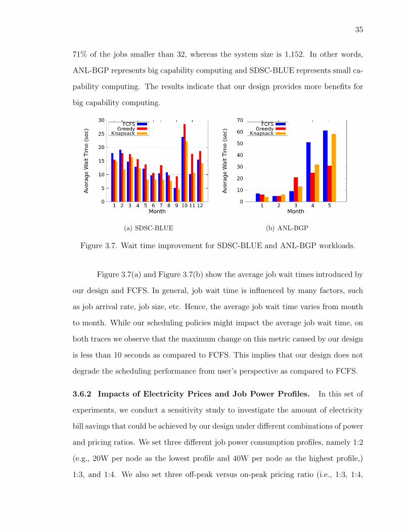
Figure 3.7. Wait time improvement for SDSC-BLUE and ANL-BGP workloads.

Figure 3.7(a) and Figure 3.7(b) show the average job wait times introduced by

our design and FCFS. In general, job wait time is influenced by many factors, such

as job arrival rate, job size, etc. Hence, the average job wait time varies from month

to month. While our scheduling policies might impact the average job wait time, on

both traces we observe that the maximum change on this metric caused by our design

is less than 10 seconds as compared to FCFS. This implies that our design does not

degrade the scheduling performance from user’s perspective as compared to FCFS.

3.6.2 Impacts of Electricity Prices and Job Power Profiles. In this set of

experiments, we conduct a sensitivity study to investigate the amount of electricity

bill savings that could be achieved by our design under different combinations of power

and pricing ratios. We set three different job power consumption profiles, namely 1:2

(e.g., 20W per node as the lowest profile and 40W per node as the highest profile,)

1:3, and 1:4. We also set three off-peak versus on-peak pricing ratio (i.e., 1:3, 1:4,

36

and 1:5). The results are summarized in Table 3.2 and 3.3.

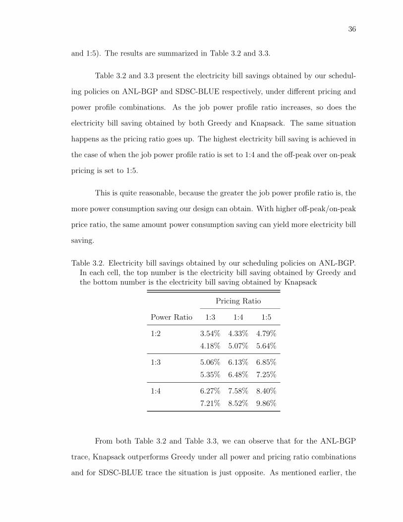
Table 3.2 and 3.3 present the electricity bill savings obtained by our schedul-

ing policies on ANL-BGP and SDSC-BLUE respectively, under different pricing and

power profile combinations. As the job power profile ratio increases, so does the

electricity bill saving obtained by both Greedy and Knapsack. The same situation

happens as the pricing ratio goes up. The highest electricity bill saving is achieved in

the case of when the job power profile ratio is set to 1:4 and the off-peak over on-peak

pricing is set to 1:5.

This is quite reasonable, because the greater the job power profile ratio is, the

more power consumption saving our design can obtain. With higher off-peak/on-peak

price ratio, the same amount power consumption saving can yield more electricity bill

saving.

Table 3.2. Electricity bill savings obtained by our scheduling policies on ANL-BGP.In each cell, the top number is the electricity bill saving obtained by Greedy andthe bottom number is the electricity bill saving obtained by Knapsack

Pricing Ratio

Power Ratio 1:3 1:4 1:5

1:2 3.54% 4.33% 4.79%

4.18% 5.07% 5.64%

1:3 5.06% 6.13% 6.85%

5.35% 6.48% 7.25%

1:4 6.27% 7.58% 8.40%

7.21% 8.52% 9.86%

From both Table 3.2 and Table 3.3, we can observe that for the ANL-BGP

trace, Knapsack outperforms Greedy under all power and pricing ratio combinations

and for SDSC-BLUE trace the situation is just opposite. As mentioned earlier, the

37

Table 3.3. Electricity bill savings obtained by our scheduling policies on SDSC-BLUE.In each cell, the top number is the electricity bill saving obtained by Greedy andthe bottom number is the electricity bill saving obtained by Knapsack

Pricing Ratio

Power Ratio 1:3 1:4 1:5

1:2 3.84% 4.84% 6.19%

2.39% 3.01% 3.85%

1:3 4.33% 5.46% 6.98%

3.16% 3.98% 5.10%

1:4 5.55% 6.98% 8.95%

3.05% 3.84% 4.92%

ANL-BGP trace contains a large percentage of large jobs. During on-peak period, the

Greedy policy always selects a job with the least power profile, whereas the Knapsack

policy often picks out a job with a small power profile under the constraint of the

available system resources. While the Knapsack policy may not schedule the job with

the least power profile, it is capable of identifying the job which consumes the least

amount of aggregated power consumption on all the nodes.

3.6.3 Impact of Scheduling Frequencies. Typically batch schedulers make

allocation decisions periodically. On production supercomputers, the scheduling fre-

quency is generally on the order of 10 to 30 seconds. Hence, in this set of experiments,

we evaluate the impact of different scheduling intervals (i.e., 10 seconds, 20 seconds,

and 30 seconds) on the amount of electricity bill savings.

Table 3.4 shows the average electricity bill savings obtained by our design

compared to the conventional FCFS with three different scheduling periods on ANL-

BGP and SDSC-BLUE. As we can see that the longer the scheduling period is, the

more electricity bill savings our design can get. This is because with a relative high job

38

arrival rate, a longer scheduling period means more system nodes can be accumulated

for job allocation at a time. As such, our design is able to allocate more low power

profiled jobs during on-peak period or more high power profiled jobs during off-peak

period, resulting in more electricity bill savings.

Table 3.4. Electricity bill Savings obtained by our scheduling policies under differentscheduling frequencies. In each cell, the top number is on ANL-BGP and thebottom number is on SDSC-BLUE.

Scheduling Policy

Frequency Greedy Knapsack

10-Second 7.49% 7.13%

4.33% 3.16%

20-Second 10.07% 8.91%

9.70% 9.80%

30-Second 17.52% 22.43%

19.69% 23.07%

Table 3.5 shows the average system utilization of ANL-BGP and SDSC-BLUE

trace under different scheduling frequencies by our design and FCFS. As we can

see that both Greedy and 0-1 Knapsack scheduling policy employed in our design

have almost no impact on the system utilization rate when the scheduling period is

10 seconds. When the scheduling period is increased to 30 seconds, some available

nodes will have to wait for a relatively long time until they are assigned to new

jobs. Thus the system utilization rate suffers slightly, however is always less than

3%. Combining the results shown in Table IV and V, it is observed that a longer

scheduling frequency can bring in more electricity bill savings, at a cost of a slightly

degraded system utilization (less than 3%).

3.6.4 Impact of Scheduling Window. The use of scheduling window, rather

39

Table 3.5. System utilization rate under different scheduling frequencies. In each cell,the top number is on ANL-BGP and the bottom number is on SDSC-BLUE.

Scheduling Policy

Frequency FCFS Greedy Knapsack

10-Second 70.0% 69.70% 69.07%

69.59% 69.53% 69.50%

20-Second 68.56% 69.03% 65.97%

68.56% 69.25% 65.06%

30-Second 63.77% 60.42% 60.84%

67.38% 68.85% 66.21%

than one by one job scheduling adopted by the conventional batch scheduling, is

a key technique of our design. Typically, an optimal window size is influenced by

many factors, in particular job arrival rate. In general, a larger window means more

opportunities for our design to make an optimal decision. However, large window size

can result in high scheduling overhead, especially Knapsack policy, since window size

is a dominant factor of its computational complexity.

We conduct a sensitivity study of scheduling window by varying its size from

10 to 200. For both traces, our results show that the variations of all three metrics are

not substantial (e.g., within 5%). More importantly, our results indicate that when

the window size is set to 10 to 30, for both traces, the variations of all three metrics

are negligible. Given the high computation overhead introduced by large window size,

a window size of 10-30 jobs is preferable for typical workload at production systems.

3.6.5 Result Summary. In summary, our trace-based experiments have shown

the following:

• Workload characteristics can impact the performance of our design in terms of

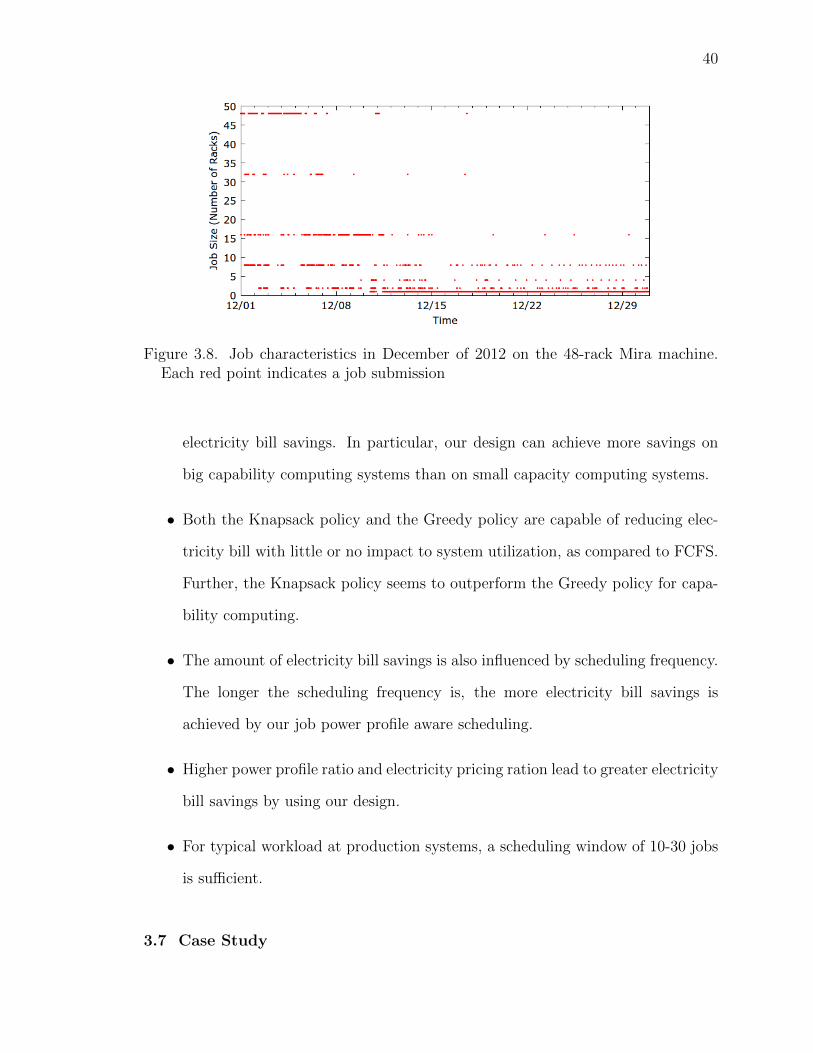
40

Figure 3.8. Job characteristics in December of 2012 on the 48-rack Mira machine.Each red point indicates a job submission

electricity bill savings. In particular, our design can achieve more savings on

big capability computing systems than on small capacity computing systems.

• Both the Knapsack policy and the Greedy policy are capable of reducing elec-

tricity bill with little or no impact to system utilization, as compared to FCFS.

Further, the Knapsack policy seems to outperform the Greedy policy for capa-

bility computing.

• The amount of electricity bill savings is also influenced by scheduling frequency.

The longer the scheduling frequency is, the more electricity bill savings is

achieved by our job power profile aware scheduling.

• Higher power profile ratio and electricity pricing ration lead to greater electricity

bill savings by using our design.

• For typical workload at production systems, a scheduling window of 10-30 jobs

is sufficient.

3.7 Case Study

41

In this section, we present a case study of using our job power aware scheduler

on Mira. We collected the job trace from the machine in December 2012. During the

month, the first half of the month were jobs for acceptance testing (hence most jobs

are large jobs) and the second half was used for early science applications from users

(hence most jobs are small sized such as single rack). There are totally 3,333 jobs

executed on the machine during the month. A summary of these jobs is described in

Figure 3.8. For each job, its power profile is extracted from the environmental log [3],

and the distribution of job power profiles is presented in Figure 3.1.

In this case study, we compare the Knapsack policy to FCFS. We apply two

scheduling frequencies, i.e. 10-second and 30-second. The scheduling window is set

to 10-second.

Figure 3.9 presents the average utilization within a day. Here system uti-

lization at each time point is calculated as the average over the month. During

the off-peak time, system utilization achieved by our scheduler is higher than that

achieved by FCFS. This is because during the off-peak time, our design attempts

to allocate jobs with high power profiles, as many as possible, by taking advantage

of low electricity pricing. During the on-peak time, FCFS achieves a slightly better

system utilization over our design. This is because our design intends to schedule

large jobs with low power profiles, leaving some idle nodes that are not sufficient for

other jobs. Nevertheless, despite some minor variation at any time instant, the daily

system utilization is not impacted or degraded by using our design.

Figure 3.10 presents the average power consumption within a day. Here power

consumption at each time point is calculated as the average over the month. During

the off-peak time, the amount of power consumed by our design is higher than that

consumed by FCFS. This phenomenon is more obvious when we switch the scheduling

frequency from 10 seconds to 30 seconds. This is reasonable as our design aims to

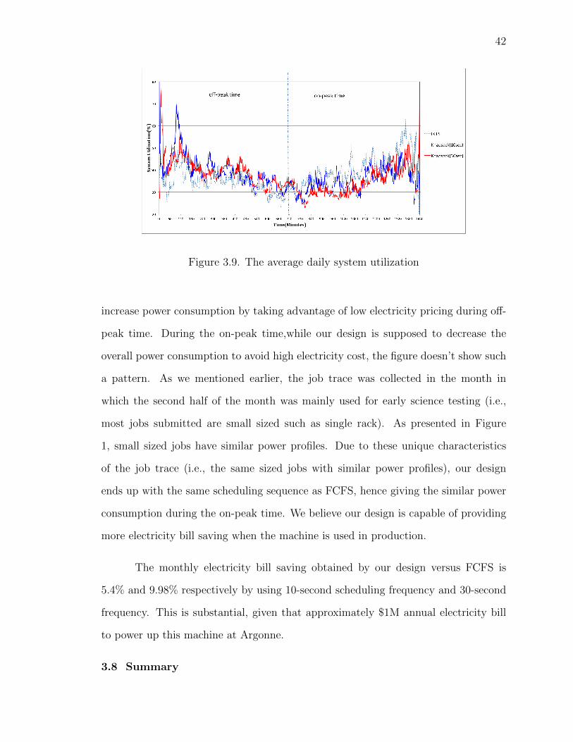
42

Figure 3.9. The average daily system utilization

increase power consumption by taking advantage of low electricity pricing during off-

peak time. During the on-peak time,while our design is supposed to decrease the

overall power consumption to avoid high electricity cost, the figure doesn’t show such

a pattern. As we mentioned earlier, the job trace was collected in the month in

which the second half of the month was mainly used for early science testing (i.e.,

most jobs submitted are small sized such as single rack). As presented in Figure

1, small sized jobs have similar power profiles. Due to these unique characteristics

of the job trace (i.e., the same sized jobs with similar power profiles), our design

ends up with the same scheduling sequence as FCFS, hence giving the similar power

consumption during the on-peak time. We believe our design is capable of providing

more electricity bill saving when the machine is used in production.

The monthly electricity bill saving obtained by our design versus FCFS is

5.4% and 9.98% respectively by using 10-second scheduling frequency and 30-second

frequency. This is substantial, given that approximately $1M annual electricity bill

to power up this machine at Argonne.

3.8 Summary

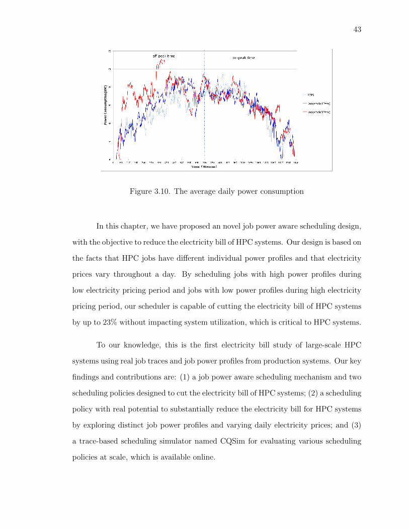
43

Figure 3.10. The average daily power consumption

In this chapter, we have proposed an novel job power aware scheduling design,

with the objective to reduce the electricity bill of HPC systems. Our design is based on

the facts that HPC jobs have different individual power profiles and that electricity

prices vary throughout a day. By scheduling jobs with high power profiles during

low electricity pricing period and jobs with low power profiles during high electricity

pricing period, our scheduler is capable of cutting the electricity bill of HPC systems

by up to 23% without impacting system utilization, which is critical to HPC systems.

To our knowledge, this is the first electricity bill study of large-scale HPC

systems using real job traces and job power profiles from production systems. Our key

findings and contributions are: (1) a job power aware scheduling mechanism and two

scheduling policies designed to cut the electricity bill of HPC systems; (2) a scheduling

policy with real potential to substantially reduce the electricity bill for HPC systems

by exploring distinct job power profiles and varying daily electricity prices; and (3)

a trace-based scheduling simulator named CQSim for evaluating various scheduling

policies at scale, which is available online.

44

CHAPTER 4

LOCALITY AWARE SCHEDULING ON TORUSCONNECTED SYSTEMS

4.1 Overview

Two scheduling strategies are commonly used on today’s torus-connected sys-

tems. One is so called partition based systems, where the scheduler assigns each

user job a compact and contiguous set of computing nodes. IBM Blue Gene se-

ries systems fall into this category [18]. This strategy is in favor of application’s

performance by preserving locality of allocated nodes and reducing network con-

tention caused by concurrently running jobs sharing network bandwidth. However,

this strategy can cause internal fragmentation (when more nodes are allocated to a

job than it requests) and external fragmentation(when sufficient nodes are available

for a request, but they can not be allocated contiguously), therefore leading to poor

system performance (e.g., low system utilization and high job response time) [20].

The other is non-contiguous allocation system, where free nodes are assigned to user

job no matter whether they are contiguous or not. Cray XT/XE series systems fall

into this category [19]. Non-contiguous allocation eliminates internal and external

fragmentation as seen in partition-based systems, thereby leading to high system

utilization. Nevertheless, it introduces other problems such as scattering applica-

tion processes all over the system. The non-contiguous node allocation can make

inter-process communication less efficient and cause network contention among con-

currently running jobs [21], thereby resulting in poor job performance especially for

those communication-intensive jobs.

Partition-based allocation achieves good job performance by sacrificing sys-

tem performance (e.g., poor system utilization), whereas non-contiguous allocation

can result in better system performance but could severely degrade performance of

45

user jobs (e.g, prolonged wait-time and run-time). As systems continue growing in

size, a fundamental problem arises: how to effectively balance job performance with

system performance on torus-connected machines? In this work, we will present a

new scheduling design combining the merits of partition based scheduling and non-

contiguous scheduling for torus-connected machines.

Strictly speaking, a job scheduling system contains two parts, namely job

prioritizing and resource allocation. Job prioritizing makes decision about the order

in which jobs are allowed to run. The decision making is based on many factors, such

as job size, job run-time, job priority, etc. Resource allocation decides a set of nodes

allocated to each incoming job. Figure 4.1 illustrates a typical job scheduling system,

where each job is retrieved from the wait queue and computing nodes are assigned

one-by-one to this job. Many supercomputers use this kind of First-Come First-Serve

(FCFS) scheduling policy. As we can see, every job gets out of the wait queue and

free nodes are assigned to the job according to node identifiers. Often the topological

characteristics and locality of system nodes are ignored. Numerically sequential nodes

may be separated from each other in the space. A well-known approach to address

the problem is processor ordering. Processor ordering usually uses space filling curve,

such as Hilbert Curve, to map the nodes of the torus onto a 1-dimensional list to

preserve locality information [27][73]. While processor ordering works well at the

beginning of scheduling, job allocation and deallocation will eventually fragment this

1-dimensional list, making it less efficient as time goes by.

In this work, we present a window-based locality-aware scheduling design. Our

design is based on two key observations. First, as shown in Figure 4.1, existing

scheduling system makes decisions in a per-job manner. Each job is dispatched to

system resources without considering subsequent jobs. While making isolating job

decision may provide a good short-term optimization, it is likely to result in poor

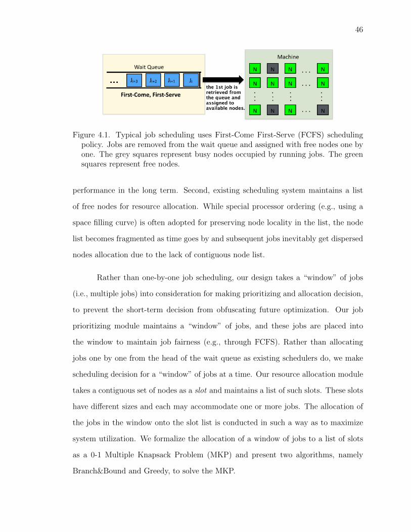
46

Figure 4.1. Typical job scheduling uses First-Come First-Serve (FCFS) schedulingpolicy. Jobs are removed from the wait queue and assigned with free nodes one byone. The grey squares represent busy nodes occupied by running jobs. The greensquares represent free nodes.

performance in the long term. Second, existing scheduling system maintains a list

of free nodes for resource allocation. While special processor ordering (e.g., using a

space filling curve) is often adopted for preserving node locality in the list, the node

list becomes fragmented as time goes by and subsequent jobs inevitably get dispersed

nodes allocation due to the lack of contiguous node list.

Rather than one-by-one job scheduling, our design takes a “window” of jobs

(i.e., multiple jobs) into consideration for making prioritizing and allocation decision,

to prevent the short-term decision from obfuscating future optimization. Our job

prioritizing module maintains a “window” of jobs, and these jobs are placed into

the window to maintain job fairness (e.g., through FCFS). Rather than allocating

jobs one by one from the head of the wait queue as existing schedulers do, we make

scheduling decision for a “window” of jobs at a time. Our resource allocation module

takes a contiguous set of nodes as a slot and maintains a list of such slots. These slots

have different sizes and each may accommodate one or more jobs. The allocation of

the jobs in the window onto the slot list is conducted in such a way as to maximize

system utilization. We formalize the allocation of a window of jobs to a list of slots

as a 0-1 Multiple Knapsack Problem (MKP) and present two algorithms, namely

Branch&Bound and Greedy, to solve the MKP.

47

We evaluate our design via extensive trace-based simulations. In this paper,

we conduct a series of experiments comparing our design against the commonly used

FCFS/EASY backfilling scheduling that is enhanced with processor ordering. Our

preliminary results demonstrate that our design can reduce average job wait time

by up to 28% and average job response time by 30%, with a slight improvement on

overall system utilization.

The structure of the chapter is as follows. Section 4.3 gives a detailed de-

scription of our window-based locality-aware scheduling design. Section 4.4 describes

the problem formalization and two scheduling algorithms implemented in our design.

Section 4.5–4.6 present our evaluation methodology, trace-based simulations by com-

paring our design against the FCFS/EASY backfilling scheduling scheme. In Section

4.2, we discuss the existing work about job scheduling and allocation on HPC systems.

Our conclusion is presented in Section 4.7.

4.2 Related Work

The most commonly used scheduling policies are FCFS combined with EASY

backfilling [67]. Under this policy, the scheduler picks a job from the head of the

wait queue and dispatches it to the available system resources. Many studies seek

to improve the performance of this classic scheduling paradigm. Tang et al. made

refinement about user’s estimated job runtime in order to make the backfilling more

efficient [66] [70]. They also designed a walltime-aware job allocation strategy, which

adjacently packs jobs that finish around the same time, in order to minimize resource

fragmentation caused by job length discrepancy [51]. And there are some other vari-

ation of FCFS/EASY backfilling proposed to optimize system performance in terms

of power consumption and energy cost [65][74]. However, none of them ever take

allocation locality into consideration when making scheduling decisions.

48

There are several studies focusing on allocation algorithms to minimize system

fragmentation. Lo et al. presented a non-contiguous allocation scheme named Multi-

ple Buddy Strategy (MBS) [75]. MBS preserves locality by allocating each job a set of

“blocks” to reduce interference between jobs, with the advantage of eliminating both

internal and external fragmentation. Each “block” consists of 2n nodes that adjacent

to each other (n with different value depends on the block size). However, the distance

between “blocks” could be too long to make the communication between processes

within the same application less efficient. MBS also needs to partition the system

into fixed number of “blocks” in advance, which is time consuming and low-efficient

for big scale systems.

Leung et al. presented allocation strategies based on space filling curves and

one dimensional packing [73]. They implemented these strategies using 2-dimensional

Hilbert curves and had an integer program for general networks. Their preliminary

experimental results show that processor locality can be preserved in massively paral-

lel supercomputers using one-dimensional allocation strategies based on space filling

curve. However, space filling curve has the limitation that it can only be applied to

system with the scale of 2n nodes in each dimension.

Albing et al. conducted study about the allocation strategies that the Cray

Application Level Placement Scheduler (ALPS) used [27]. The job allocation in Cray

Linux Environment (CLE) operating system is managed by ALPS, which works from

a list of available nodes and assigns those nodes in sequence from this list to jobs.

However, ALPS does not make changes or calculations when making allocation deci-

sions. It just simply works off the ordered list, however that is ordered. They claimed

that the ordered list can be obtained by using either Hilbert curve or simply sorting

the nodes based on their spacial coordinates in the system.

There are other studies focusing on allocation algorithms to improve the per-

49

formance of user jobs. Pascual et al. proposed an allocation strategy that aiming to

assign a contiguous allocation to each job, in order to improve communication per-

formance [21]. However, this strategy results in severe scheduling inefficiency due to

increased system fragmentation. They reduced this adverse effect by using a relaxed

version called quasi-contiguous allocation strategy.

Another related work is online bin packing. In the bin packing strategy, the

objective is to pack a set of items with given sizes into bins. Each bin has a fixed

capacity and cannot be assigned to items whose total size exceeds this capacity. The

goal is to minimize the number of bins used. The off-line version is NP-hard [76] and

bin packing was one of the first problems to be studied in terms of both online and

offline approximability [77][78].

This work has two major difference as compared to the above literatures. First,

rather than one-by-one job scheduling as most existing schedulers do [27][75][21],

our design takes a “window” of jobs (i.e.,multiple jobs) into consideration for job

prioritizing and resource allocation. Second, our resource management module takes

a contiguous set of nodes as a slot and maintains a list of such slots. The slot list

is updated dynamically when job being allocated/deallocated in the system. The

allocation of the jobs in the window onto the slot list is conducted in such a way as to

maximize system utilization. This is different from the existing job allocation schemes

that work off a ordered list, which loses the spacial information of the torus-connected

system.

4.3 Design Overview

Figure 4.2 gives an overview of our window-based locality-aware job scheduling

design. Our design contains two key parts. The job prioritizing module maintains a

“window” of jobs that are retrieved from the wait queue to insure job fairness. Rather

50

Figure 4.2. Overview of our window-based locality-aware scheduling design. The jobprioritizing module maintains a “window” of jobs retrieved from the wait queue,and the resource management module keeps a list of slots. Each slot represents acontiguous set of available nodes. Our scheduling design allocates a “window” ofjobs to a list of slots at a time.

than dispatching jobs one by one as existing schedulers do, we dispatch multiple jobs

at a time. Unlike existing scheduling design, the resource management module is

responsible for organizing the available nodes into a set of slots. Each slot contains a

contiguous set of free nodes. Here, contiguity refers to the adjacency of nodes’ original

positions in torus-connected system. These slots may have different sizes. A new slot

appears when a job releases the nodes it was assigned. The newly released nodes

merge with other free neighboring nodes to form up a new slot with growing size. A

slot disappears when it (or part of it) is assigned to a job. If the job’s requirement

only takes part of a slot, the remaining part becomes a new slot. The slot list is

updated when a job is allocated or deallocated. The resource management module

needs to get feedback from the system right after a job being allocated/deallocated

to update the status of the slot list. The allocation of the jobs in the window onto

the slot list is conducted in such a way as to maximize system utilization.

Using window-based design can balance job fairness and system performance.

In our design, rather than allocating jobs one by one from the front of the wait

51

queue, the scheduler takes all the jobs in the window and make prioritizing decision

for them at a time. The selection of jobs from wait queue to the window is based on

certain scheduling rule (e.g., job arrival time in case of using FCFS policy), thereby

guaranteeing job fairness. With the information of both jobs and slots, the scheduler

aims to make an optimal decision in terms of allocating the jobs to the slots. In the

following section, we will present our detailed scheduling strategy.

4.4 Scheduling Strategy

Our scheduling strategy contains two parts. We first formalize the resource

allocation problem into a 0-1 Multiple Knapsack Problem (MKP), and then present

two algorithms to solve the MKP.

4.4.1 MKP Formalization. We consider each slot as a knapsack and the jobs

in the window are the items waiting to be put into the knapsacks. Suppose J =

{J1, J2, J3, ..., Jn} is a set of n jobs in the window. Each job Jj has weight wj, with

profit pj. And K = {K1, K2, K3, ..., Km} is a set of m knapsacks; each knapsack Ki

with the capacity of Ci. So, we want to select m disjoint subsets of jobs so that

the total profit of the selected jobs is a maximum, and each subset can be put into

different knapsack whose capacity is no less than the total weight of jobs in the subset.

Formally,

Max z =m∑i=1

n∑j=1

pj · xij (4.1)

which is subject to the following constraints:

n∑j=1

xij · wj ≤ Ci, i ∈ {1, 2, ...,m} (4.2)

52

m∑i=1

xij ≤ 1, j ∈ {1, 2, ..., n} (4.3)

xij ∈ {0, 1}, i ∈ {1, 2, ...,m}; j ∈ {1, 2, ..., n} (4.4)

where

xij =

1 if job j is put into knapsack i;

0 otherwise

(4.5)

When m=1, Multiple Knapsack problem reduces to the 0-1 knapsack problem.

In our model, we can assume that

pj and Ci are positive integers, (4.6)

wj ≤ maxi∈ICi, ∀j ∈ {1, 2, ..., n}, (4.7)

Ci ≥ minj∈Jwj, ∀i ∈ {1, 2, ...,m}, (4.8)

n∑j=1

wj > Ci, ∀i ∈ {1, 2, ...,m}, (4.9)

53

In our model, it is guaranteed that assumption 4.6 can’t be violated since the

definitions of job’s profit and weight in our maximization problem are both its size.

And the capacity of knapsack is the size of the slots, which can never be negative. If

there is a job j violating assumption 4.7, which means it requires too many nodes to

be accommodated in any knapsack, it will be hold until a slot appears which contains

enough free nodes. In our experiments, we found that this would only prolong the

big jobs’ wait time less than 10%. If a knapsack violates assumption 4.8, then it will

be taken as system fragmentation. Finally, observe that if m > n then the (m − n)

knapsacks of smallest capacity will not be included in this formalization.

The window size should be set based on the system’s workload such that a large

window is preferred when job arrival rate is high. For typical workload at production

supercomputers, we find a window of size 5 makes a good tradeoff between scheduling

quality and scheduling overhead.

4.4.2 Algorithms. In this work, we develop two scheduling algorithms. The first

is Branch and Bound Algorithm. The second is Greedy Algorithm. We will discuss

the details about both scheduling algorithms in this section.

Branch and Bound (B&B) is a general algorithm for finding optimal solutions

of discrete and combinatorial optimization problems [79]. In our model, we can control

the size of window to limit the number of jobs in the MKP model so that the overhead

of the B&B algorithm can be acceptable in terms of time and space complexity. In

our experiment, we set window size to 5, which means only the first 5 jobs in the wait

queue are considered in our MKP model. The computation time for solving the MKP

problem with 5 jobs is affordable for the scheduler. (The scheduler makes scheduling

decision periodically with a interval from 10 to 30 seconds.)

In this algorithm, successive levels of the branch-decision tree are constructed

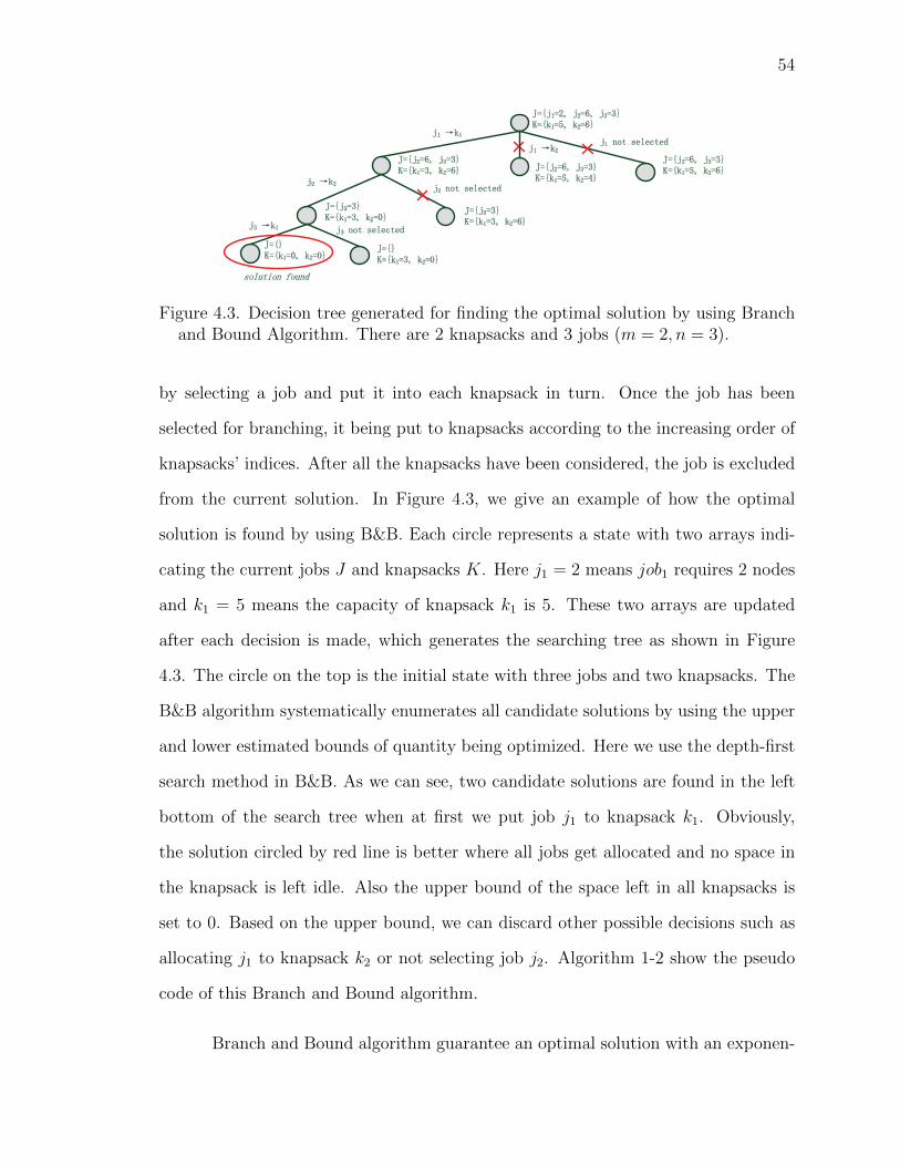
54

Figure 4.3. Decision tree generated for finding the optimal solution by using Branchand Bound Algorithm. There are 2 knapsacks and 3 jobs (m = 2, n = 3).

by selecting a job and put it into each knapsack in turn. Once the job has been

selected for branching, it being put to knapsacks according to the increasing order of

knapsacks’ indices. After all the knapsacks have been considered, the job is excluded

from the current solution. In Figure 4.3, we give an example of how the optimal

solution is found by using B&B. Each circle represents a state with two arrays indi-

cating the current jobs J and knapsacks K. Here j1 = 2 means job1 requires 2 nodes

and k1 = 5 means the capacity of knapsack k1 is 5. These two arrays are updated

after each decision is made, which generates the searching tree as shown in Figure

4.3. The circle on the top is the initial state with three jobs and two knapsacks. The

B&B algorithm systematically enumerates all candidate solutions by using the upper

and lower estimated bounds of quantity being optimized. Here we use the depth-first

search method in B&B. As we can see, two candidate solutions are found in the left

bottom of the search tree when at first we put job j1 to knapsack k1. Obviously,

the solution circled by red line is better where all jobs get allocated and no space in

the knapsack is left idle. Also the upper bound of the space left in all knapsacks is

set to 0. Based on the upper bound, we can discard other possible decisions such as

allocating j1 to knapsack k2 or not selecting job j2. Algorithm 1-2 show the pseudo

code of this Branch and Bound algorithm.

Branch and Bound algorithm guarantee an optimal solution with an exponen-

55

Algorithm 4.1 Branch & Bound

E = new (node), this is the dummy start node

H = new (Heap), this is a max-heap for our maximization problem

while true do

if E is a final leaf then

E is an optimal solution;

print out the path from E to the root;

return;

end if

Branch(E);

if H is empty then

No solution;

return;

end if

E = delete-top(H);

end while

Algorithm 4.2 Branch

Generate all the children of E;

Compute the approximate cost value Ci of each child;

Insert each child into the heap H;

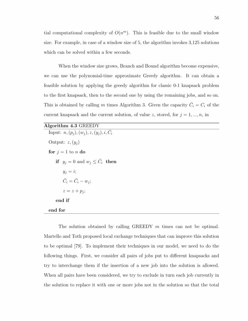
56

tial computational complexity of O(nm). This is feasible due to the small window

size. For example, in case of a window size of 5, the algorithm invokes 3,125 solutions

which can be solved within a few seconds.

When the window size grows, Branch and Bound algorithm become expensive,

we can use the polynomial-time approximate Greedy algorithm. It can obtain a

feasible solution by applying the greedy algorithm for classic 0-1 knapsack problem

to the first knapsack, then to the second one by using the remaining jobs, and so on.

This is obtained by calling m times Algorithm 3. Given the capacity Ci = Ci of the

current knapsack and the current solution, of value z, stored, for j = 1, ..., n, in

Algorithm 4.3 GREEDY

Input: n, (pj), (wj), z, (yj), i, Ci

Output: z, (yj)

for j = 1 to n do

if yj = 0 and wj ≤ Ci then

yj = i;

Ci = Ci − wj;

z = z + pj;

end if

end for

The solution obtained by calling GREEDY m times can not be optimal.

Martello and Toth proposed local exchange techniques that can improve this solution

to be optimal [79]. To implement their techniques in our model, we need to do the

following things. First, we consider all pairs of jobs put to different knapsacks and

try to interchange them if the insertion of a new job into the solution is allowed.

When all pairs have been considered, we try to exclude in turn each job currently in

the solution to replace it with one or more jobs not in the solution so that the total

57

profit is increased. Greedy algorithm has a linear time complexity, i.e., O(n). And

the interchange takes O(n) since it only happens when a new job enters the solution.

Hence, using GREEDY to find the optimal solution will cost no more than O(n2)

time.

yj =

1 if job j is currently unassigned;

index of the knapsack it is assigned to.

(4.10)

4.4.3 An Example. We have the following example to illustrate the difference

between our design and the default scheduler using FCFS/EASY backfilling. Here we

assume five jobs A, B, C, D, E are submitted and waiting in the queue. The system

consists of 20 nodes in total, and the current available nodes are: 1, 2, 3, 6, 7, 8,

9, 10, 11, 15, 16, 17, 18, 19, 20. The nodes do not appear in this list (indexes

are 4, 5, 12, 13, 14) are occupied by jobs that are still running. The FCFS/EASY

backfilling scheme used by the default scheduler will cut a chunk of six nodes from

start of this list for job A, which means node 1, 2, 3, 6, 7, 8 are assigned to job A.

And then sequentially, nodes 9, 10, 11, 15 will be assigned to B; 16, 17, 18 to C;

19 to D.

Apparently, this scheme doesn’t deliver the best allocation. First, job A and B

get a non-contiguous node sets, which means their allocation are fragmented. Node 20

is left idle, and job E has not been satisfied since the available nodes is not enough to

satisfy its requirement. Under this default scheduling scheme, the scheduling sequence

will always be 〈A, B, C, D, E〉, in spite of the current status of node list and each

job’s size.

Our design first puts these five jobs into the window according to their arrival

order, which is A, B, C, D, E. Then it checks the status of the slot list (formed based

58

on system nodes contiguity) and find out how many slots is available. In our example,

there are three such slots, 1, 2, 3, 6, 7, 8, 9, 10, 11, 15, 16, 17, 18, 19, 20. Then

based on the size of these slots and each job’s size, our design will use B&B or Greedy

algorithm to make the following scheduling decision. First, it puts job C into the first

slot(assign nodes 1, 2, 3 to C); then put job A into the second slot (6, 7, 8, 9, 10,

11 to A); 15, 16, 17, 18 to B; 19, 20 to E. Apparently, our design can guarantee

that every job gets a compact allocation while maintain high system utilization.

Figure 4.4 pictorially illustrates this example to highlight the difference be-

tween our design and the default scheduler using FCFS policy. As it shows, there are

20 nodes in the node list, the grey ones are been occupied by current running jobs.

The subfigure A in 4.4 is the scheduling result obtained by the default scheduler.

It fragments the allocation for job A(with size 6) and job B (with size 4), leaving

node No.20 idle and job E (with size 2) unallocated. In subfigure B, our design can

guarantee that every job gets a compact allocation.

Figure 4.4. Scheduling result comparison between the default scheduler and ourdesign. The default scheduler (Subfigure A) makes job prioritizing sequence as〈A,B,C,D〉, and the allocation for job A and B are fragmented, node 20 is leftidle. Our design (Subfigure B) can make optimization so that every job gets acompact allocation and no node is left idle. The prioritizing sequence obtained byour design is 〈C,A,B,E〉.

4.5 Evaluation Methodology

59

We conduct a series of experiments using the traces described in Section 4.5.2

to evaluate our design as against the default scheduler using FCFS/EASY backfilling.

FCFS/EASY backfilling is the most commonly used scheduling policy on production

supercomputers [66][51]. In the rest of the paper, we use B&B, Greedy, and Default

to denote our algorithms and the default one. This section describes our evaluation

methodology and the experimental results will be presented in the next section.

4.5.1 CQSim: Trace-based Scheduling Simulator. Simulation is an integral

part of our evaluation of various allocation policies as well as their aggregate effects on

system utilization, job’s wait time and response time. We have developed a simulator

named CQSim to evaluate our design at scale. The simulator is written in Python,

and is formed by several modules such as job module, node module, scheduling policy

module, etc. Each module is implemented as a class. The design principles are

reusability, extensibility, and efficiency. The simulator takes job events from the

trace, and an event could be job submission, start, end, and other events. Based on

these events, the simulator emulates job submission, allocation, and execution based

on specific scheduling and allocation policies. CQsim is open source, and is available

to the community [41].

4.5.2 Job Traces. In this work, we use two real workload traces collected from

production supercomputers to evaluate our design. The objective of using multiple

traces is to quantify the performance of our design when dealing jobs and systems

with different characteristics. The first trace we used is from a machine named Blue

Horizon at the San Diego Supercomputer Center (denoted as SDSC-BLUE in the

paper), which contains 4,830 jobs. The second trace we used is from a IBM Blue

Gene/P system named Intrepid at Argonne National Laboratory (denoted as ANL-

Intrepid in the paper) [42]. This trace contains 2,612 jobs. Figure 4.5 summarizes

job size distribution of these traces. ANL-Intrepid is used to represent capability

60

computing where jobs require a large amount of computing nodes for solving large-

scale problems, whereas SDSC-BLUE is used to represent capacity computing where

the system is utilized to solve a large number of small-sized problems.

Figure 4.5. Job size distribution of ANL-Intrepid and SDSC-BLUE

4.5.3 Evaluation Metrics. We use three scheduling metrics for evaluation.

• System Utilization Rate. This metric denotes the ratio of the node-hours used

by jobs to the total elapsed system node-hours. Specifically, let T be the total

elapsed time for J jobs, ci be the completion time for job i and si be its the

start time, and ni be the size of job i, then system utilization rate is calculated

as ∑0≤i≤J (ci − si) · ni

N · T(4.11)

• Average Job Wait Time. For each job, its wait time refers to the time elapsed

between the moment it is submitted and the moment it is allocated to run.

This metric is calculated as the average across all the jobs submitted to the

61

system. This metric is a user-centric metric, measuring scheduling performance

from user’s perspective.

Twait = tstart − tarrive (4.12)

• Average Job Response time. Response time refers to the amount of time it take

when each job is submitted until it ends, which equals to its wait time plus its

run time.

Tresponse = Trun + Twait (4.13)

4.6 Experiment Results

We conduct a series of experiments on the traces described in Section 4.5.2 to

evaluate our design as against the default scheduler which uses FCFS/EASY back-

filling policy.

In our experiments, the scheduler makes scheduling decisions every 30 seconds.

To make the scheduler responsive, the window size is set to 5 so that the time cost

for B&B algorithm to solve the MKP is affordable (e.g., in seconds). We assume

there are β percentage jobs in each trace are sensitive to the contiguity of allocation.

Existing studies show that job runtime is influenced by resource allocation, and the

variability introduced by different allocations could be as high as 70% [4][80]. In our

experiments, we use a parameter α to denote this impact. For a job that is sensitive to

the contiguity of resource allocation, we assume its runtime on a contiguous allocation

is about α percentage shorter than on a non-contiguous allocation. We conduct a

series of sensitivity study to evaluate our design under a variety of configurations. In

the following experiments, both β and α are set to 10%, 20%, 30%, 40%, 50%.

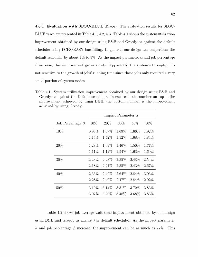
62

4.6.1 Evaluation with SDSC-BLUE Trace. The evaluation results for SDSC-

BLUE trace are presented in Table 4.1, 4.2, 4.3. Table 4.1 shows the system utilization

improvement obtained by our design using B&B and Greedy as against the default

scheduler using FCFS/EASY backfilling. In general, our design can outperform the

default scheduler by about 1% to 3%. As the impact parameter α and job percentage

β increase, this improvement grows slowly. Apparently, the system’s throughput is

not sensitive to the growth of jobs’ running time since those jobs only required a very

small portion of system nodes.

Table 4.1. System utilization improvement obtained by our design using B&B andGreedy as against the Default scheduler. In each cell, the number on top is theimprovement achieved by using B&B, the bottom number is the improvementachieved by using Greedy.

Impact Parameter α

Job Percentage β 10% 20% 30% 40% 50%

10% 0.98% 1.37% 1.69% 1.66% 1.92%

1.15% 1.42% 1.52% 1.68% 1.84%

20% 1.28% 1.09% 1.46% 1.50% 1.77%

1.11% 1.12% 1.54% 1.63% 1.69%

30% 2.23% 2.23% 2.35% 2.48% 2.54%

2.18% 2.21% 2.35% 2.43% 2.67%

40% 2.36% 2.49% 2.64% 2.84% 3.03%

2.28% 2.49% 2.47% 2.84% 2.92%

50% 3.10% 3.14% 3.31% 3.72% 3.83%

3.07% 3.20% 3.48% 3.68% 3.83%

Table 4.2 shows job average wait time improvement obtained by our design

using B&B and Greedy as against the default scheduler. As the impact parameter

α and job percentage β increase, the improvement can be as much as 27%. This

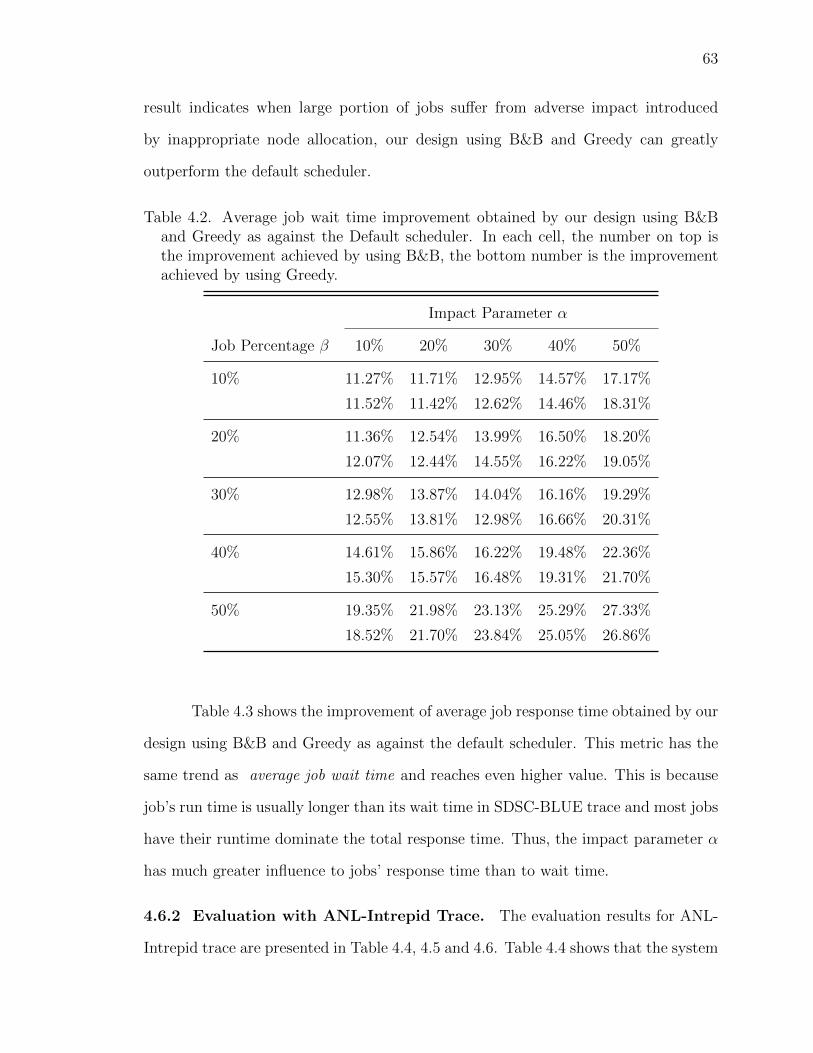
63

result indicates when large portion of jobs suffer from adverse impact introduced

by inappropriate node allocation, our design using B&B and Greedy can greatly

outperform the default scheduler.

Table 4.2. Average job wait time improvement obtained by our design using B&Band Greedy as against the Default scheduler. In each cell, the number on top isthe improvement achieved by using B&B, the bottom number is the improvementachieved by using Greedy.

Impact Parameter α

Job Percentage β 10% 20% 30% 40% 50%

10% 11.27% 11.71% 12.95% 14.57% 17.17%

11.52% 11.42% 12.62% 14.46% 18.31%

20% 11.36% 12.54% 13.99% 16.50% 18.20%

12.07% 12.44% 14.55% 16.22% 19.05%

30% 12.98% 13.87% 14.04% 16.16% 19.29%

12.55% 13.81% 12.98% 16.66% 20.31%

40% 14.61% 15.86% 16.22% 19.48% 22.36%

15.30% 15.57% 16.48% 19.31% 21.70%

50% 19.35% 21.98% 23.13% 25.29% 27.33%

18.52% 21.70% 23.84% 25.05% 26.86%

Table 4.3 shows the improvement of average job response time obtained by our

design using B&B and Greedy as against the default scheduler. This metric has the

same trend as average job wait time and reaches even higher value. This is because

job’s run time is usually longer than its wait time in SDSC-BLUE trace and most jobs

have their runtime dominate the total response time. Thus, the impact parameter α

has much greater influence to jobs’ response time than to wait time.

4.6.2 Evaluation with ANL-Intrepid Trace. The evaluation results for ANL-

Intrepid trace are presented in Table 4.4, 4.5 and 4.6. Table 4.4 shows that the system

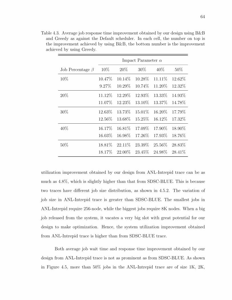
64

Table 4.3. Average job response time improvement obtained by our design using B&Band Greedy as against the Default scheduler. In each cell, the number on top isthe improvement achieved by using B&B, the bottom number is the improvementachieved by using Greedy.

Impact Parameter α

Job Percentage β 10% 20% 30% 40% 50%

10% 10.47% 10.14% 10.28% 11.11% 12.62%

9.27% 10.29% 10.74% 11.20% 12.32%

20% 11.12% 12.29% 12.93% 13.33% 14.93%

11.07% 12.23% 13.10% 13.37% 14.78%

30% 12.63% 13.73% 15.01% 16.20% 17.79%

12.56% 13.68% 15.25% 16.12% 17.32%

40% 16.17% 16.81% 17.09% 17.90% 18.90%

16.03% 16.98% 17.26% 17.93% 18.76%

50% 18.81% 22.11% 23.39% 25.56% 28.83%

18.17% 22.00% 23.45% 24.98% 28.41%

utilization improvement obtained by our design from ANL-Intrepid trace can be as

much as 4.8%, which is slightly higher than that from SDSC-BLUE. This is because

two traces have different job size distribution, as shown in 4.5.2. The variation of

job size in ANL-Intrepid trace is greater than SDSC-BLUE. The smallest jobs in

ANL-Intrepid require 256-node, while the biggest jobs require 8K nodes. When a big

job released from the system, it vacates a very big slot with great potential for our

design to make optimization. Hence, the system utilization improvement obtained

from ANL-Intrepid trace is higher than from SDSC-BLUE trace.

Both average job wait time and response time improvement obtained by our

design from ANL-Intrepid trace is not as prominent as from SDSC-BLUE. As shown

in Figure 4.5, more than 50% jobs in the ANL-Intrepid trace are of size 1K, 2K,

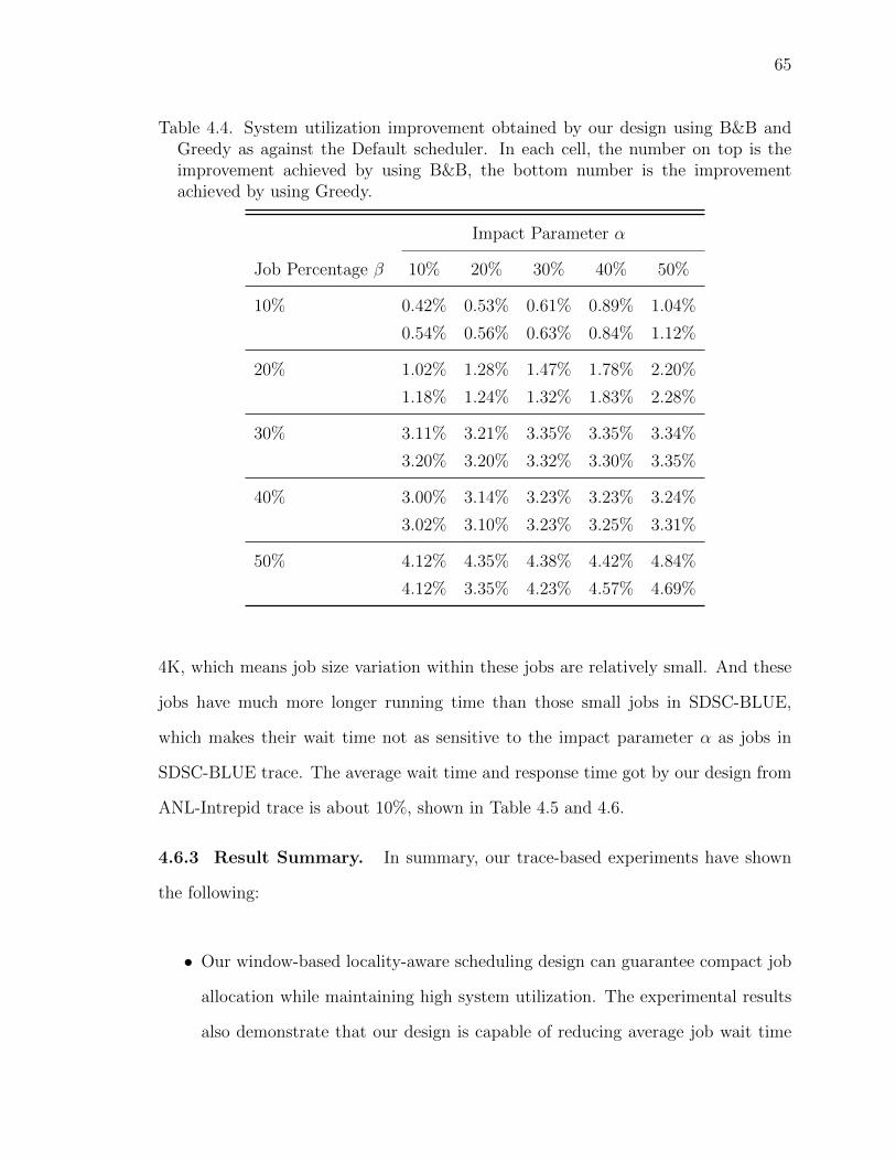
65

Table 4.4. System utilization improvement obtained by our design using B&B andGreedy as against the Default scheduler. In each cell, the number on top is theimprovement achieved by using B&B, the bottom number is the improvementachieved by using Greedy.

Impact Parameter α

Job Percentage β 10% 20% 30% 40% 50%

10% 0.42% 0.53% 0.61% 0.89% 1.04%

0.54% 0.56% 0.63% 0.84% 1.12%

20% 1.02% 1.28% 1.47% 1.78% 2.20%

1.18% 1.24% 1.32% 1.83% 2.28%

30% 3.11% 3.21% 3.35% 3.35% 3.34%

3.20% 3.20% 3.32% 3.30% 3.35%

40% 3.00% 3.14% 3.23% 3.23% 3.24%

3.02% 3.10% 3.23% 3.25% 3.31%

50% 4.12% 4.35% 4.38% 4.42% 4.84%

4.12% 3.35% 4.23% 4.57% 4.69%

4K, which means job size variation within these jobs are relatively small. And these

jobs have much more longer running time than those small jobs in SDSC-BLUE,

which makes their wait time not as sensitive to the impact parameter α as jobs in

SDSC-BLUE trace. The average wait time and response time got by our design from

ANL-Intrepid trace is about 10%, shown in Table 4.5 and 4.6.

4.6.3 Result Summary. In summary, our trace-based experiments have shown

the following:

• Our window-based locality-aware scheduling design can guarantee compact job

allocation while maintaining high system utilization. The experimental results

also demonstrate that our design is capable of reducing average job wait time

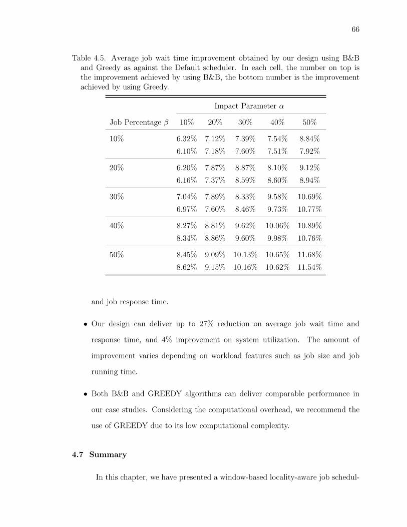
66

Table 4.5. Average job wait time improvement obtained by our design using B&Band Greedy as against the Default scheduler. In each cell, the number on top isthe improvement achieved by using B&B, the bottom number is the improvementachieved by using Greedy.

Impact Parameter α

Job Percentage β 10% 20% 30% 40% 50%

10% 6.32% 7.12% 7.39% 7.54% 8.84%

6.10% 7.18% 7.60% 7.51% 7.92%

20% 6.20% 7.87% 8.87% 8.10% 9.12%

6.16% 7.37% 8.59% 8.60% 8.94%

30% 7.04% 7.89% 8.33% 9.58% 10.69%

6.97% 7.60% 8.46% 9.73% 10.77%

40% 8.27% 8.81% 9.62% 10.06% 10.89%

8.34% 8.86% 9.60% 9.98% 10.76%

50% 8.45% 9.09% 10.13% 10.65% 11.68%

8.62% 9.15% 10.16% 10.62% 11.54%

and job response time.

• Our design can deliver up to 27% reduction on average job wait time and

response time, and 4% improvement on system utilization. The amount of

improvement varies depending on workload features such as job size and job

running time.

• Both B&B and GREEDY algorithms can deliver comparable performance in

our case studies. Considering the computational overhead, we recommend the

use of GREEDY due to its low computational complexity.

4.7 Summary

In this chapter, we have presented a window-based locality-aware job schedul-

67

Table 4.6. Average job response time improvement obtained by our design using B&Band Greedy as against the Default scheduler. In each cell, the number on top isthe improvement achieved by using B&B, the bottom number is the improvementachieved by using Greedy.

Impact Parameter α

Job Percentage β 10% 20% 30% 40% 50%

10% 3.81% 4.09% 4.87% 5.05% 5.76%

4.00% 4.26% 4.76% 4.93% 5.81%

20% 5.16% 5.53% 5.89% 6.76% 8.91%

4.03% 4.46% 5.76% 6.76% 8.80%

30% 5.03% 5.52% 6.76% 7.90% 8.93%

5.16% 5.81% 6.86% 7.67% 9.00%

40% 6.08% 7.52% 7.73% 8.89% 9.54%

5.70% 7.35% 7.58% 8.74% 9.26%

50% 6.16% 7.09% 9.12% 9.90% 10.85%

6.05% 7.10% 9.23% 9.85% 10.68%

ing design for torus-connected system. Our goal is to balance job performance with

system performance. Our design has three novel features. First, rather than one-

by-one job scheduling, our design takes a “window” of jobs (i.e.,multiple jobs) into

consideration for job prioritizing and resource allocation. Second, our design main-

tains a list of slots to preserve node contiguity information for resource allocation.

Finally, we formulate a 0-1 Multiple Knapsack problem to describe our scheduling de-

cision making and present two algorithms to solve the problem. Preliminary results

based on trace-based simulation demonstrate our design can reduce average job wait

time by up to 28% and average job response time by 30%, with a slight improvement

on overall system utilization.

68

CHAPTER 5

JOB INTERFERENCE ANALYSIS ON TORUSCONNECTED SYSTEMS

5.1 Overview

On the widely used torus network topology [23–25], two job placement policies

are commonly used. In contiguous placement, each job gets a compact and contiguous

set of computing nodes, as shown in Figure 5.1(a). The partition-based placement

adopted in the Blue Gene series of supercomputers is a prominent example [26].

Contiguous placement favors application performance through exclusive resource al-

location and the locality that implies. However, contiguous placement can cause both

internal fragmentation (when more nodes are allocated to a job than it requests) and

external fragmentation (when sufficient nodes are available for a request, but they

can not be allocated contiguously), therefore leading to lower system utilization than

is otherwise possible. On the other hand, noncontiguous placement, adopted by the

Cray XT/XE series [27], assigns free nodes to jobs regardless of contiguity, although

of course efforts are made to maximize locality. Figure 5.1(b) shows an example

of noncontiguous placement. While eliminating the internal and external fragmen-

tation seen in contiguous placement systems, noncontiguous placement introduces

contention among jobs due to the interleaving of the jobs’ nodes, particularly for

communication-intensive jobs [4].

We envision that future HPC systems will be equipped with flexible job place-

ment mechanisms that combine the best of both contiguous and noncontiguous poli-

cies. Such a mechanism would take into account the shared resource needs (e.g.,

network resources) of jobs when making scheduling and allocation decisions. With

the knowledge and analysis of job communication patterns, one can identify which

jobs require exclusive network and compact allocation and to what degree. Then,

69

rather than allocating each job in a “know-nothing” manner, one may customize

the job placement policy so that, for example, only the jobs with stringent network

needs are given compact, isolated allocations, resulting in maximized utilization and

minimized perceivable resource contention effects.

(a) Contiguous (b) Non-contiguous

Figure 5.1. Multiple jobs running concurrently with different allocations. Each job isrepresented by a specific color. a) shows the effect of contiguous allocation, whichreduce the inter-job interference. b) shows non-contiguous allocation, which mayintroduce both intra and inter-job interferences.

In this chapter, we focus on an in-depth analysis of intra- and interjob commu-

nication interference with different job placements on torus-connected HPC systems.

Although our analysis is based on torus networks, the ideas conveyed in this work are

applicable to networks with different topologies.

We selected three signature applications from the DOE Design Forward Project

[31] to conduct a detailed study about the communication behavior of parallel ap-

plications. We use a sophisticated simulation toolkit named CODES (standing for

Co-Design of Multi-layer Exascale Storage Architectures) [32] as a research vehicle to

evaluate the performance of these applications with various allocations in a controlled

environment. We then analyze the intra- and interjob interference by simulating these

applications running concurrently with different allocations. We believe the insights

presented in this work can be useful for the design of future HPC batch schedulers

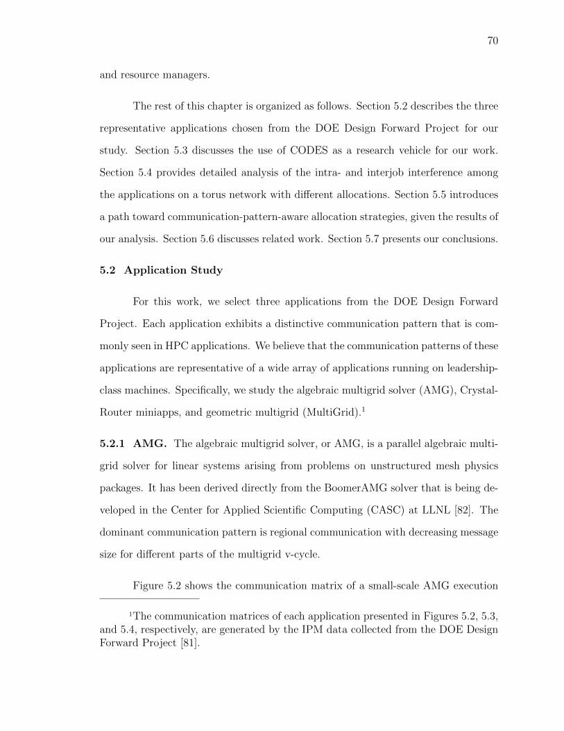
70

and resource managers.

The rest of this chapter is organized as follows. Section 5.2 describes the three

representative applications chosen from the DOE Design Forward Project for our

study. Section 5.3 discusses the use of CODES as a research vehicle for our work.

Section 5.4 provides detailed analysis of the intra- and interjob interference among

the applications on a torus network with different allocations. Section 5.5 introduces

a path toward communication-pattern-aware allocation strategies, given the results of

our analysis. Section 5.6 discusses related work. Section 5.7 presents our conclusions.

5.2 Application Study

For this work, we select three applications from the DOE Design Forward

Project. Each application exhibits a distinctive communication pattern that is com-

monly seen in HPC applications. We believe that the communication patterns of these

applications are representative of a wide array of applications running on leadership-

class machines. Specifically, we study the algebraic multigrid solver (AMG), Crystal-

Router miniapps, and geometric multigrid (MultiGrid).1

5.2.1 AMG. The algebraic multigrid solver, or AMG, is a parallel algebraic multi-

grid solver for linear systems arising from problems on unstructured mesh physics

packages. It has been derived directly from the BoomerAMG solver that is being de-

veloped in the Center for Applied Scientific Computing (CASC) at LLNL [82]. The

dominant communication pattern is regional communication with decreasing message

size for different parts of the multigrid v-cycle.

Figure 5.2 shows the communication matrix of a small-scale AMG execution

1The communication matrices of each application presented in Figures 5.2, 5.3,and 5.4, respectively, are generated by the IPM data collected from the DOE DesignForward Project [81].

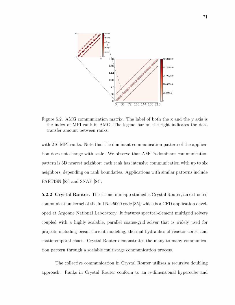
71

Figure 5.2. AMG communication matrix. The label of both the x and the y axis isthe index of MPI rank in AMG. The legend bar on the right indicates the datatransfer amount between ranks.

with 216 MPI ranks. Note that the dominant communication pattern of the applica-

tion does not change with scale. We observe that AMG’s dominant communication

pattern is 3D nearest neighbor: each rank has intensive communication with up to six

neighbors, depending on rank boundaries. Applications with similar patterns include

PARTISN [83] and SNAP [84].

5.2.2 Crystal Router. The second miniapp studied is Crystal Router, an extracted

communication kernel of the full Nek5000 code [85], which is a CFD application devel-

oped at Argonne National Laboratory. It features spectral-element multigrid solvers

coupled with a highly scalable, parallel coarse-grid solver that is widely used for

projects including ocean current modeling, thermal hydraulics of reactor cores, and

spatiotemporal chaos. Crystal Router demonstrates the many-to-many communica-

tion pattern through a scalable multistage communication process.

The collective communication in Crystal Router utilizes a recursive doubling

approach. Ranks in Crystal Router conform to an n-dimensional hypercube and

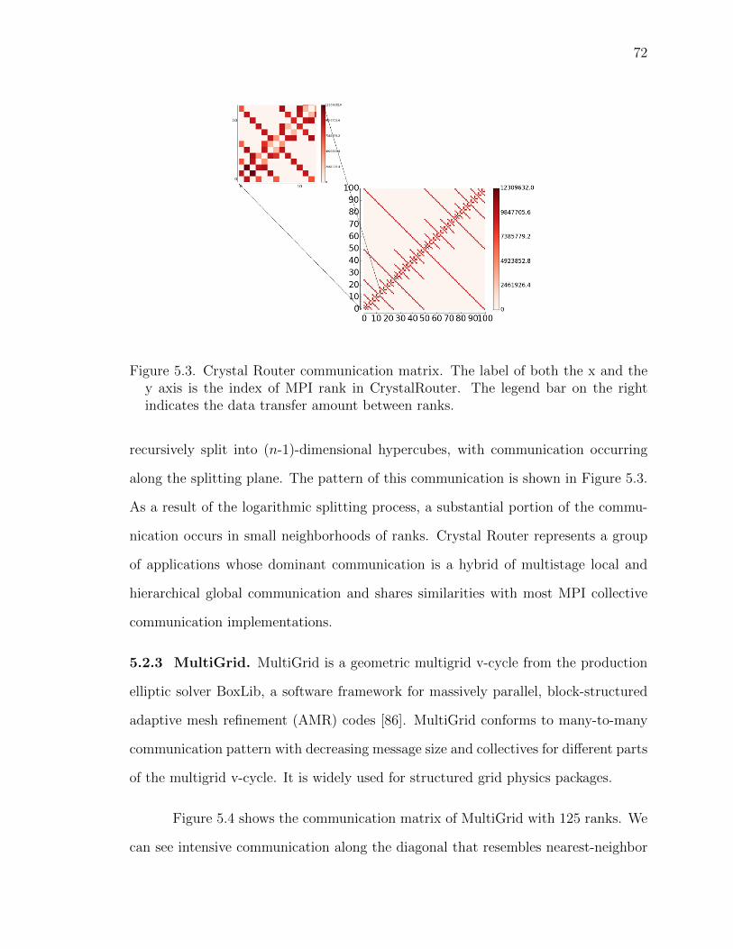
72

Figure 5.3. Crystal Router communication matrix. The label of both the x and they axis is the index of MPI rank in CrystalRouter. The legend bar on the rightindicates the data transfer amount between ranks.

recursively split into (n-1)-dimensional hypercubes, with communication occurring

along the splitting plane. The pattern of this communication is shown in Figure 5.3.

As a result of the logarithmic splitting process, a substantial portion of the commu-

nication occurs in small neighborhoods of ranks. Crystal Router represents a group

of applications whose dominant communication is a hybrid of multistage local and

hierarchical global communication and shares similarities with most MPI collective

communication implementations.

5.2.3 MultiGrid. MultiGrid is a geometric multigrid v-cycle from the production

elliptic solver BoxLib, a software framework for massively parallel, block-structured

adaptive mesh refinement (AMR) codes [86]. MultiGrid conforms to many-to-many

communication pattern with decreasing message size and collectives for different parts

of the multigrid v-cycle. It is widely used for structured grid physics packages.

Figure 5.4 shows the communication matrix of MultiGrid with 125 ranks. We

can see intensive communication along the diagonal that resembles nearest-neighbor

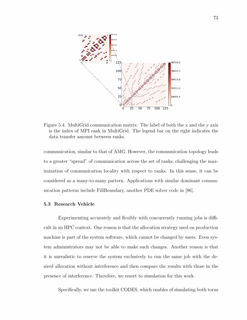
73

Figure 5.4. MultiGrid communication matrix. The label of both the x and the y axisis the index of MPI rank in MultiGrid. The legend bar on the right indicates thedata transfer amount between ranks.

communication, similar to that of AMG. However, the communication topology leads

to a greater “spread” of communication across the set of ranks, challenging the max-

imization of communication locality with respect to ranks. In this sense, it can be

considered as a many-to-many pattern. Applications with similar dominant commu-

nication patterns include FillBoundary, another PDE solver code in [86].

5.3 Research Vehicle

Experimenting accurately and flexibly with concurrently running jobs is diffi-

cult in an HPC context. One reason is that the allocation strategy used on production

machine is part of the system software, which cannot be changed by users. Even sys-

tem administrators may not be able to make such changes. Another reason is that

it is unrealistic to reserve the system exclusively to run the same job with the de-

sired allocation without interference and then compare the results with those in the

presence of interference. Therefore, we resort to simulation for this work.

Specifically, we use the toolkit CODES, which enables of simulating both torus

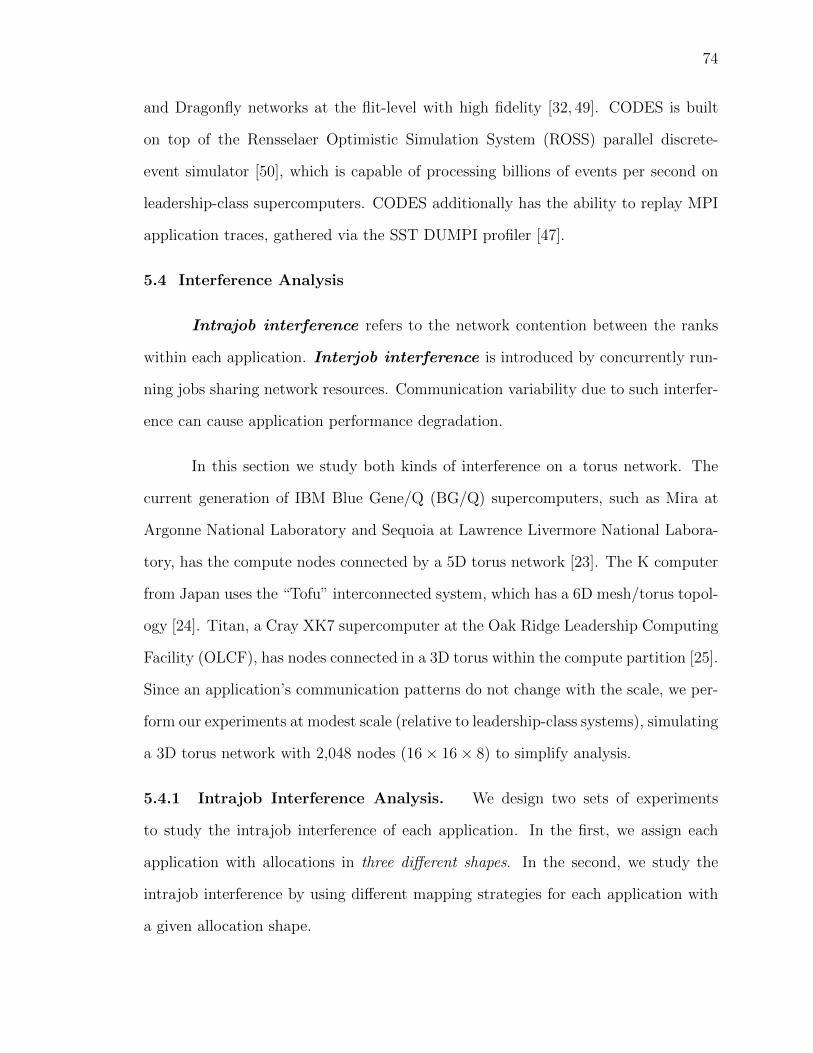
74

and Dragonfly networks at the flit-level with high fidelity [32, 49]. CODES is built

on top of the Rensselaer Optimistic Simulation System (ROSS) parallel discrete-

event simulator [50], which is capable of processing billions of events per second on

leadership-class supercomputers. CODES additionally has the ability to replay MPI

application traces, gathered via the SST DUMPI profiler [47].

5.4 Interference Analysis

Intrajob interference refers to the network contention between the ranks

within each application. Interjob interference is introduced by concurrently run-

ning jobs sharing network resources. Communication variability due to such interfer-

ence can cause application performance degradation.

In this section we study both kinds of interference on a torus network. The

current generation of IBM Blue Gene/Q (BG/Q) supercomputers, such as Mira at

Argonne National Laboratory and Sequoia at Lawrence Livermore National Labora-

tory, has the compute nodes connected by a 5D torus network [23]. The K computer

from Japan uses the “Tofu” interconnected system, which has a 6D mesh/torus topol-

ogy [24]. Titan, a Cray XK7 supercomputer at the Oak Ridge Leadership Computing

Facility (OLCF), has nodes connected in a 3D torus within the compute partition [25].

Since an application’s communication patterns do not change with the scale, we per-

form our experiments at modest scale (relative to leadership-class systems), simulating

a 3D torus network with 2,048 nodes (16× 16× 8) to simplify analysis.

5.4.1 Intrajob Interference Analysis. We design two sets of experiments

to study the intrajob interference of each application. In the first, we assign each

application with allocations in three different shapes. In the second, we study the

intrajob interference by using different mapping strategies for each application with

a given allocation shape.

75

5.4.1.1 Allocation Shapes Study. In the allocation shapes experiment, we

select three shapes commonly seen on the 3D torus network: 3D balanced cube, 3D

unbalanced cube, and 2D mesh, as shown in Figure 5.5.

The 3D balanced cube, shown in red in Figure 5.5, can guarantee the minimum

average pairwise distance within the allocation. Some research studies [4,73] indicate

that compact allocation can guarantee jobs with better performance. To evaluate the

compactness of the allocation, they use a variety of metrics such as average pairwise

distance, diameter, and contiguity. In this work, we select the 3D balanced cube as

the most compact allocation on a 3D torus network.

The 3D unbalanced cube, shown in green in Figure 5.5, is a rectangular prism,

which is a possible allocation shape on systems with asymmetric networks. For exam-

ple, Cray XE6/XK7 systems are 3D tori with Gemini routers. The network connec-

tions in the y-direction have only half the bandwidth of the cables used in the x and z

directions. In order to take advantage of the faster links in the x and z directions, job

allocation favors the X-Z plane [87]. Our torus network in this study is symmetric.

The 2D mesh, shown in blue in Figure 5.5, can be cut out from a single layer of

the 3D torus. The 2D mesh is a common allocation shape on torus networks for both

contiguous and noncontiguous placement policies. For example, Cray’s Application

Level Placement Scheduler (ALPS) indexes all compute nodes in the torus into a

list and allocates by simply going through that list [27]. When the list is obtained

by sorting the nodes based on their spatial coordinates in the torus, the resulting

allocations form 2D meshes. The IBM Blue Gene/Q supercomputer Mira at the

Argonne Leadership Computing Facility also allows its allocation partition to be

configured as a mesh [88].

Figure 5.6(a) shows that AMG with a 3D nearest-neighbor communication

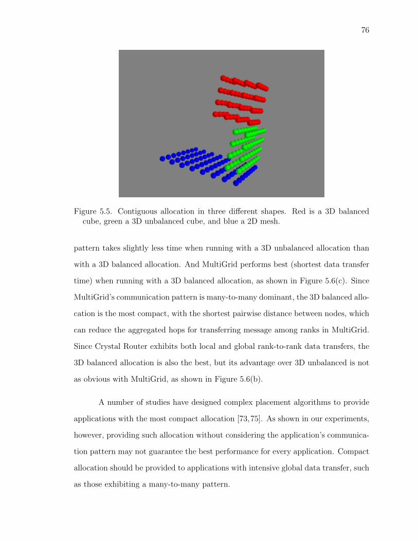
76

Figure 5.5. Contiguous allocation in three different shapes. Red is a 3D balancedcube, green a 3D unbalanced cube, and blue a 2D mesh.

pattern takes slightly less time when running with a 3D unbalanced allocation than

with a 3D balanced allocation. And MultiGrid performs best (shortest data transfer

time) when running with a 3D balanced allocation, as shown in Figure 5.6(c). Since

MultiGrid’s communication pattern is many-to-many dominant, the 3D balanced allo-

cation is the most compact, with the shortest pairwise distance between nodes, which

can reduce the aggregated hops for transferring message among ranks in MultiGrid.

Since Crystal Router exhibits both local and global rank-to-rank data transfers, the

3D balanced allocation is also the best, but its advantage over 3D unbalanced is not

as obvious with MultiGrid, as shown in Figure 5.6(b).

A number of studies have designed complex placement algorithms to provide

applications with the most compact allocation [73,75]. As shown in our experiments,

however, providing such allocation without considering the application’s communica-

tion pattern may not guarantee the best performance for every application. Compact

allocation should be provided to applications with intensive global data transfer, such

as those exhibiting a many-to-many pattern.

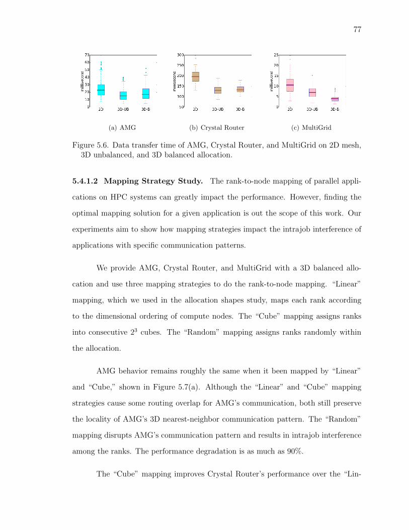
77

(a) AMG (b) Crystal Router (c) MultiGrid

Figure 5.6. Data transfer time of AMG, Crystal Router, and MultiGrid on 2D mesh,3D unbalanced, and 3D balanced allocation.

5.4.1.2 Mapping Strategy Study. The rank-to-node mapping of parallel appli-

cations on HPC systems can greatly impact the performance. However, finding the

optimal mapping solution for a given application is out the scope of this work. Our

experiments aim to show how mapping strategies impact the intrajob interference of

applications with specific communication patterns.

We provide AMG, Crystal Router, and MultiGrid with a 3D balanced allo-

cation and use three mapping strategies to do the rank-to-node mapping. “Linear”

mapping, which we used in the allocation shapes study, maps each rank according

to the dimensional ordering of compute nodes. The “Cube” mapping assigns ranks

into consecutive 23 cubes. The “Random” mapping assigns ranks randomly within

the allocation.

AMG behavior remains roughly the same when it been mapped by “Linear”

and “Cube,” shown in Figure 5.7(a). Although the “Linear” and “Cube” mapping

strategies cause some routing overlap for AMG’s communication, both still preserve

the locality of AMG’s 3D nearest-neighbor communication pattern. The “Random”

mapping disrupts AMG’s communication pattern and results in intrajob interference

among the ranks. The performance degradation is as much as 90%.

The “Cube” mapping improves Crystal Router’s performance over the “Lin-

78

ear” mapping by up to 10% on average, shown in Figure 5.7(b). This improvement is

due to the fact that the global data transfer in Crystal Router takes fewer hops with

the “Cube” mapping. The “Random” mapping for Crystal Router results in poor

locality across all ranks on average and makes their communication less efficient. The

“Cube” mapping benefits MultiGrid’s many-to-many communication. Because of the

small amount of data transfered among ranks in MultiGrid, however, the “Cube”

mapping fails to exhibit a significant advantage. The “Random” mapping causes

little degradation for the same reason, shown in Figure 5.7(c).

(a) AMG (b) Crystal Router (c) MultiGrid

Figure 5.7. Data transfer time of AMG, Crystal Router, and MultiGrid on 3D bal-anced allocation using different mapping strategies.

5.4.2 Interjob Interference Analysis. Interjob interference has been identified as

one of the major culprits responsible for application’s performance variability [4,89].

Interjob interference is a more prominent issue for systems adopting noncontiguous

placement policies than for systems with a contiguous policy. Application communi-

cation times have been demonstrated to vary from 36% less to 69% more as a result

of job interference when applications are running concurrently with noncontiguous

allocations [4].

We allocate each application with a noncontiguous policy and run them con-

currently on the same network. The compute nodes belonging to different jobs are

interleaved. To study the impact of different allocation unit sizes on applications’

interjob interference, we conduct experiments with unit size of 16, 8, and 2, shown

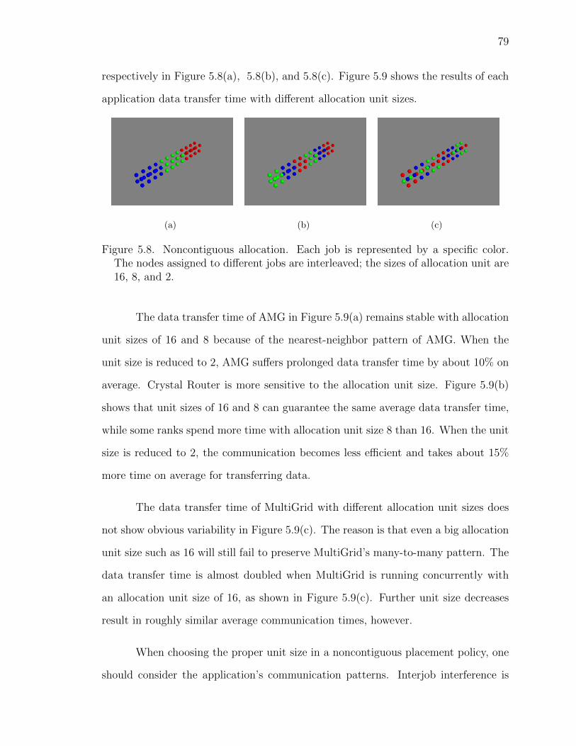
79

respectively in Figure 5.8(a), 5.8(b), and 5.8(c). Figure 5.9 shows the results of each

application data transfer time with different allocation unit sizes.

(a) (b) (c)

Figure 5.8. Noncontiguous allocation. Each job is represented by a specific color.The nodes assigned to different jobs are interleaved; the sizes of allocation unit are16, 8, and 2.

The data transfer time of AMG in Figure 5.9(a) remains stable with allocation

unit sizes of 16 and 8 because of the nearest-neighbor pattern of AMG. When the

unit size is reduced to 2, AMG suffers prolonged data transfer time by about 10% on

average. Crystal Router is more sensitive to the allocation unit size. Figure 5.9(b)

shows that unit sizes of 16 and 8 can guarantee the same average data transfer time,

while some ranks spend more time with allocation unit size 8 than 16. When the unit

size is reduced to 2, the communication becomes less efficient and takes about 15%

more time on average for transferring data.

The data transfer time of MultiGrid with different allocation unit sizes does

not show obvious variability in Figure 5.9(c). The reason is that even a big allocation

unit size such as 16 will still fail to preserve MultiGrid’s many-to-many pattern. The

data transfer time is almost doubled when MultiGrid is running concurrently with

an allocation unit size of 16, as shown in Figure 5.9(c). Further unit size decreases

result in roughly similar average communication times, however.

When choosing the proper unit size in a noncontiguous placement policy, one

should consider the application’s communication patterns. Interjob interference is

80

inevitable in noncontiguous-based systems, but unit sizes big enough to preserve the

neighborhood communication of the application will alleviate such interference and

improve job performance.

(a) AMG (b) Crystal Router (c)

Figure 5.9. Interjob interference study: “cont” indicates three applications runningside by side concurrently on the same network with contiguous allocation. Tostudy the impact of noncontiguous allocation on interjob interference, applicationsare run concurrently with interleaved allocations of different unit sizes, namely, 16node, 8 node, and 2 node.

5.4.3 Results Summary. Based on our simulation study, we make following ob-

servations.

• Compact allocation may not be necessary for every application.

• The applications dominated by nearest-neighbor communications exhibit rela-

tively stable performance under different allocation shapes as long as the allo-

cation exhibits some degree of locality.

• The applications dominated with many-to-many communication exhibit better

performance with more compact allocations (e.g., 3D balanced).

• A good rank-to-node mapping strategy can greatly improve an application per-

formance when a specific allocation is given.

• An optimal size for allocation units should be determined according to an ap-

plication’s dominant communication pattern. In general, a unit size should be

81

large enough to accommodate neighboring communication in the application.

• Interjob interference is inevitable with a noncontiguous allocation. However,

choosing the proper allocation unit size with communication pattern awareness

can help alleviate the resulting negative effects.

5.5 Discussion

The results shown in the preceding sections provide insights for the design of a

smart and flexible job placement policy. By scrutinizing the communication behavior

of jobs, we can identify their dominant communication patterns and pinpoint locality

needs. With such knowledge about communication patterns, we can analyze the

possible interference between jobs and take precautions to alleviate interference when

making placement decisions.

When an application with intensive many-to-many communication is submit-

ted to the system, the scheduler should provide it with a compact node allocation and

exclusive network resources. Compact allocation can guarantee the shortest pairwise

distance between all the ranks. Additionally, the exclusive network provision will

prevent other jobs from sharing network resources, thus eliminating the performance

degradation due to interference.

Arguably, however, not every application requires compact allocation and ex-

clusive network provisioning. As we demonstrate in our study, applications whose

dominant communication pattern contains intensive “neighborhood communication”

such as nearest neighbor may not benefit from compact allocation and exclusive net-

work provision. Applications such as AMG can run with a noncontiguous node al-

location without significant performance degradation, as long as the allocation unit

can accommodate their rank-rank locality.

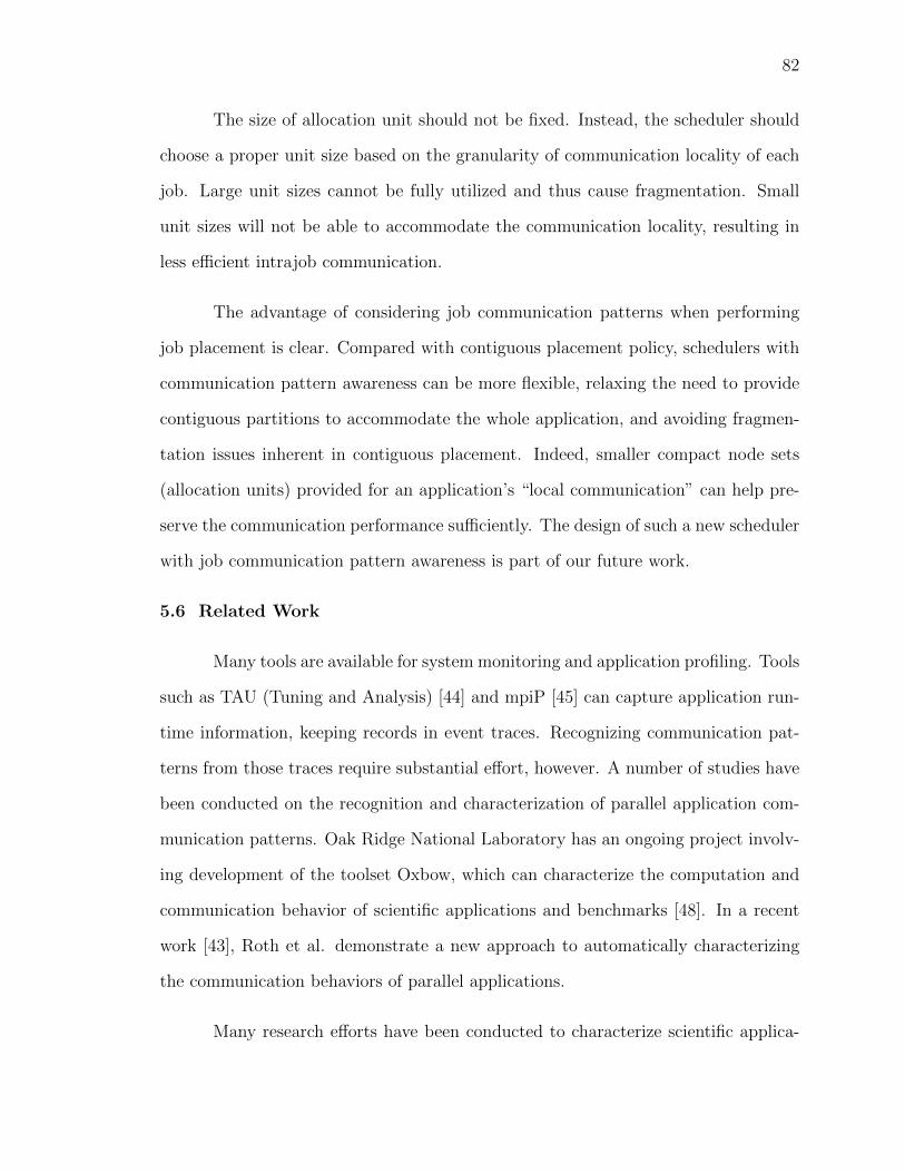
82

The size of allocation unit should not be fixed. Instead, the scheduler should

choose a proper unit size based on the granularity of communication locality of each

job. Large unit sizes cannot be fully utilized and thus cause fragmentation. Small

unit sizes will not be able to accommodate the communication locality, resulting in

less efficient intrajob communication.

The advantage of considering job communication patterns when performing

job placement is clear. Compared with contiguous placement policy, schedulers with

communication pattern awareness can be more flexible, relaxing the need to provide

contiguous partitions to accommodate the whole application, and avoiding fragmen-

tation issues inherent in contiguous placement. Indeed, smaller compact node sets

(allocation units) provided for an application’s “local communication” can help pre-

serve the communication performance sufficiently. The design of such a new scheduler

with job communication pattern awareness is part of our future work.

5.6 Related Work

Many tools are available for system monitoring and application profiling. Tools

such as TAU (Tuning and Analysis) [44] and mpiP [45] can capture application run-

time information, keeping records in event traces. Recognizing communication pat-

terns from those traces require substantial effort, however. A number of studies have

been conducted on the recognition and characterization of parallel application com-

munication patterns. Oak Ridge National Laboratory has an ongoing project involv-

ing development of the toolset Oxbow, which can characterize the computation and

communication behavior of scientific applications and benchmarks [48]. In a recent

work [43], Roth et al. demonstrate a new approach to automatically characterizing

the communication behaviors of parallel applications.

Many research efforts have been conducted to characterize scientific applica-

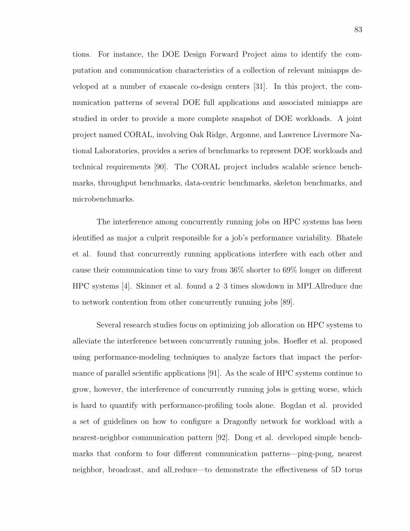
83

tions. For instance, the DOE Design Forward Project aims to identify the com-

putation and communication characteristics of a collection of relevant miniapps de-

veloped at a number of exascale co-design centers [31]. In this project, the com-

munication patterns of several DOE full applications and associated miniapps are

studied in order to provide a more complete snapshot of DOE workloads. A joint

project named CORAL, involving Oak Ridge, Argonne, and Lawrence Livermore Na-

tional Laboratories, provides a series of benchmarks to represent DOE workloads and

technical requirements [90]. The CORAL project includes scalable science bench-

marks, throughput benchmarks, data-centric benchmarks, skeleton benchmarks, and

microbenchmarks.

The interference among concurrently running jobs on HPC systems has been

identified as major a culprit responsible for a job’s performance variability. Bhatele

et al. found that concurrently running applications interfere with each other and

cause their communication time to vary from 36% shorter to 69% longer on different

HPC systems [4]. Skinner et al. found a 2–3 times slowdown in MPI Allreduce due

to network contention from other concurrently running jobs [89].

Several research studies focus on optimizing job allocation on HPC systems to

alleviate the interference between concurrently running jobs. Hoefler et al. proposed

using performance-modeling techniques to analyze factors that impact the perfor-

mance of parallel scientific applications [91]. As the scale of HPC systems continue to

grow, however, the interference of concurrently running jobs is getting worse, which

is hard to quantify with performance-profiling tools alone. Bogdan et al. provided

a set of guidelines on how to configure a Dragonfly network for workload with a

nearest-neighbor communication pattern [92]. Dong et al. developed simple bench-

marks that conform to four different communication patterns—ping-pong, nearest

neighbor, broadcast, and all reduce—to demonstrate the effectiveness of 5D torus

84

networks [93].

We differentiate our work from these activities in the following ways. First, we

focus on the dominant communication patterns rather than any specific application.

We believe this focus can provide a guideline for other research work. Second, we ex-

plore both intra- and interjob interference between concurrently running jobs, whereas

similar work such as [4] focuses on a single application’s performance degradation due

to network contention. Third, we analyze the impact of different placement strate-

gies on a job’s communication behaviors, identifying preferred placement strategies

for each application with a specific dominant communication pattern. Based on our

study, we claim that future batch schedulers should take job communication patterns

into consideration for placement decision making.

5.7 Conclusions

In this chapter, we have studied the communication behavior of three parallel

applications: AMG, Crystal Router, and MultiGrid. Each application has a distinc-

tive communication pattern, which can be representative for a whole range of jobs

commonly seen in HPC environment. We have used the CODES toolkit to simulate

the running of these applications on a torus network.

We have analyzed the intra- and interjob interference by simulating three ap-

plications running both independently and concurrently. Based on our comprehensive

experiments, we make six observations.

1. Compact allocation may not be necessary for every application.

2. The applications dominated by nearest-neighbor communications exhibit rela-

tively stable performance under different allocation shapes as long as the allo-

cation exhibit some degree of locality.

85

3. The applications dominated with many-to-many communication exhibit better

performance with more compact allocations (e.g., 3D balanced).

4. A good rank-to-node mapping strategy can greatly improve an application’s

performance when a specific allocation is given.

5. An optimal size for allocation units should be determined according to an ap-

plication’s dominant communication pattern. In general, a unit size should be

large enough to accommodate neighboring communication in the application.

6. Interjob interference is inevitable in noncontiguous allocation. However, choos-

ing the proper allocation unit size with communication pattern awareness can

help alleviate the resulting negative effects.

We believe that the findings in this work can provide valuable guidance for

HPC batch schedulers and resource managers to make flexible job allocations. Rather

than using predefined partitions or a noncontiguous placement policy, future HPC

systems should assign resources to each job based on job communication patterns.

86

CHAPTER 6

JOB INTERFERENCE ANALYSIS ON DRAGONFLYCONNECTED SYSTEMS

6.1 Overview

Low-latency and high-bandwidth interconnect networks play a critical role in

ensuring HPC system performance. The high-radix, low-diameter dragonfly topology

can lower the overall cost of the interconnect, improve network bandwidth and reduce

packet latency [35], making it a very promising choice for building supercomputers

with millions of cores. Even with such powerful networks, intelligent job placement

is of paramount importance to the efficient use of dragonfly connected systems [5,7].

Intelligent job placement plays critical role in exploring the full potential of such high

performance networks.

In this chapter, we study the implications of contention for shared network

links in the context of multiple HPC applications running on dragonfly systems when

different job placement and routing configurations are in use. Our analyses focus

on the overall network performance as well as the performance of concurrently ex-

ecuting applications in the presence of network contention. We use the same three

applications discussed in section 5.2 and analyze the interference among them. For

each application, we first examine its performance with two job placement policies

and three routing policies. And we make the following observations through extensive

simulations.

• Concurrently running applications on a dragonfly network interfere with each

other when they share network resources. Communication-intensive applica-

tions “bully” their less intensive peers and obtain performance improvement at

the expense of less intensive ones.

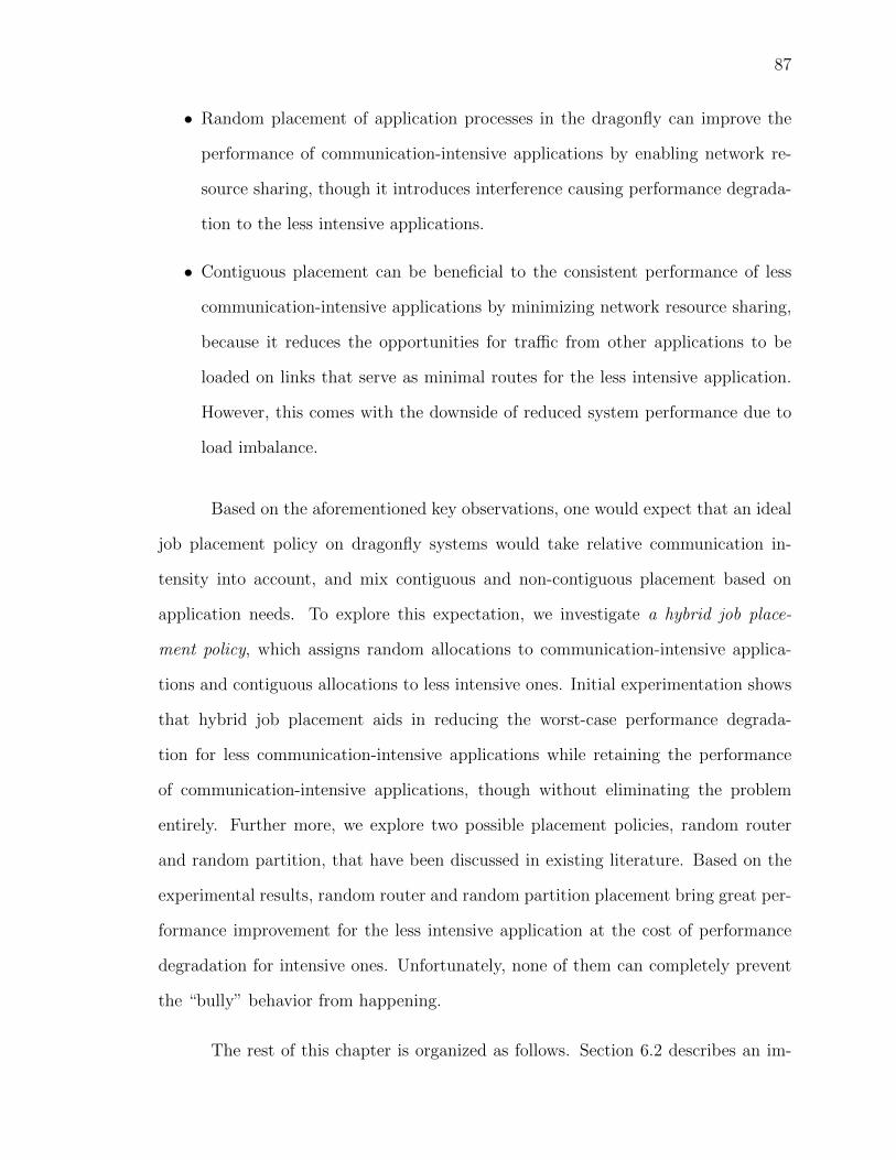
87

• Random placement of application processes in the dragonfly can improve the

performance of communication-intensive applications by enabling network re-

source sharing, though it introduces interference causing performance degrada-

tion to the less intensive applications.

• Contiguous placement can be beneficial to the consistent performance of less

communication-intensive applications by minimizing network resource sharing,

because it reduces the opportunities for traffic from other applications to be

loaded on links that serve as minimal routes for the less intensive application.

However, this comes with the downside of reduced system performance due to

load imbalance.

Based on the aforementioned key observations, one would expect that an ideal

job placement policy on dragonfly systems would take relative communication in-

tensity into account, and mix contiguous and non-contiguous placement based on

application needs. To explore this expectation, we investigate a hybrid job place-

ment policy, which assigns random allocations to communication-intensive applica-

tions and contiguous allocations to less intensive ones. Initial experimentation shows

that hybrid job placement aids in reducing the worst-case performance degrada-

tion for less communication-intensive applications while retaining the performance

of communication-intensive applications, though without eliminating the problem

entirely. Further more, we explore two possible placement policies, random router

and random partition, that have been discussed in existing literature. Based on the

experimental results, random router and random partition placement bring great per-

formance improvement for the less intensive application at the cost of performance

degradation for intensive ones. Unfortunately, none of them can completely prevent

the “bully” behavior from happening.

The rest of this chapter is organized as follows. Section 6.2 describes an im-

88

plementation of the dragonfly network, introduces the placement policies and routing

policies. Section 6.3 discusses the use of CODES as a research vehicle and three rep-

resentative applications from the DOE Design Forward Project. Section 6.4 presents

the observations and analysis of three applications running on a dragonfly network

with different placement and routing configurations. Section 6.5 validates the obser-

vations we obtain from previous section. Section 6.6 presents a alternative placement

policy for the dragonfly network. Section 6.7 explores two other possible job place-

ment policies that have been discussed in previous literature. Section 6.8 discusses

the related work. Finally, the conclusion is presented in Section 6.9.

6.2 Background

In this section, we review the dragonfly topology, including the placement and

routing policies examined in previous work.

6.2.1 Dragonfly Network. The dragonfly is a two-level hierarchical topology,

consisting of several groups connected by all-to-all links [94]. Each group consists of

a routers connected via all-to-all local channels. For each router, p compute nodes

are attached to it via terminal links, while h links are used as global channels for

intergroup connections. The resulting radix of each router is k = a + h + p − 1.

Different computing centers could choose different values for a, h, p when deploying

their dragonfly network. The adoption of proper a, h, p involves many factors such

as system scale, building cost and workload characteristics.

It is recommended that for load balancing purposes, a proper dragonfly con-

figuration should follow a = 2p = 2h [94]. According to this configuration, the total

number of groups, denoted as g in the dragonfly network would be g = a ∗ h+ 1, the

total number of compute nodes denoted as N in the network would be N = p ∗ a ∗ g.

In this work, we focus on the dragonfly topology that follow this configuration. An

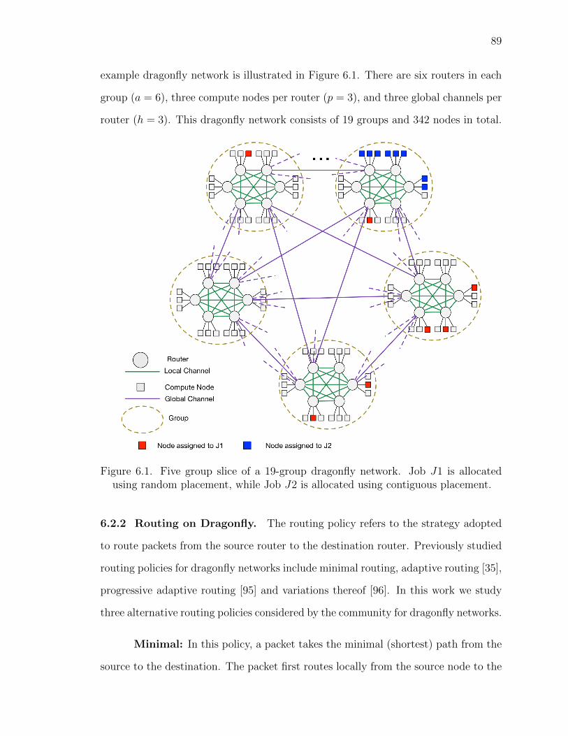
89

example dragonfly network is illustrated in Figure 6.1. There are six routers in each

group (a = 6), three compute nodes per router (p = 3), and three global channels per

router (h = 3). This dragonfly network consists of 19 groups and 342 nodes in total.

Figure 6.1. Five group slice of a 19-group dragonfly network. Job J1 is allocatedusing random placement, while Job J2 is allocated using contiguous placement.

6.2.2 Routing on Dragonfly. The routing policy refers to the strategy adopted

to route packets from the source router to the destination router. Previously studied

routing policies for dragonfly networks include minimal routing, adaptive routing [35],

progressive adaptive routing [95] and variations thereof [96]. In this work we study

three alternative routing policies considered by the community for dragonfly networks.

Minimal: In this policy, a packet takes the minimal (shortest) path from the

source to the destination. The packet first routes locally from the source node to the

90

global channel leading to the destination group. It traverses the global channel to

the destination group and routes locally to the destination node. Minimal routing

can guarantee the minimum hops a packet takes from the source to the destination.

However, it usually results in congestion along the minimal paths.

Adaptive: In this policy, the path a packet takes will be adaptively chosen

between minimal and non-minimal paths, depending on the congestion situation along

those paths. For the non-minimal path, an intermediate router in a separate group will

be randomly chosen. The packet is forwarded to the intermediate router, connecting

the source and destination groups through two separate minimal paths. Adaptive

routing can avoid hot-spots in the presence of congestion and collapses to minimal

routing otherwise.

Progressive Adaptive: As opposed to adaptive routing, the decision to

adaptively route a packet is continually re-evaluated within the source group un-

til a non-minimal route is chosen; the re-evaluation does not occur in intermediate

groups [95]. Progressive adaptive routing is capable of handling scenarios where the

minimal route is congested but the source router has not been informed yet.

6.2.3 Job Placement on Dragonfly. For a parallel application requiring mul-

tiple compute nodes, the job placement policy refers to the way of assigning the

required number of nodes to the application by system software such as the batch

scheduler [97]. In this work, we study two alternative placement policies considered

by the community for dragonfly systems:

Random Placement: In this policy, an application gets the required num-

ber of nodes randomly from the available nodes in the system. As illustrated in

Figure 6.1, J1 is randomly allocated nodes attached to different routers in differ-

ent groups. Routers may be shared by different applications and more routers are

91

involved in serving each application when random placement is in use. Random place-

ment can distribute the tasks of an application uniformly across the network to avoid

the possible local congestion.

Contiguous Placement: In this policy, the compute nodes are assigned to

an application consecutively. The assignment first fills up a group, then crosses group

boundaries as necessary. As illustrated in Figure 6.1, J2 is allocated eight nodes by

contiguous placement. Contiguous placement confines the tasks of an application into

the same group and uses the minimum number of routers to serve each application,

which may result in local network congestion and increase the possibility of hot-spots.

6.3 Methodology

Configurable dragonfly networks that allow us to perform the exploration pre-

sented in this paper are hard to come by for the time being. Even with access to

systems with such networks, job placement and routing policies are part of system

configuration, which is impossible for users to make changes at will [5, 6, 10, 98].

Therefore, we resort to simulation in our work.

6.3.1 Simulation Tool. We utilize the CODES simulation toolkit (Co-Design of

Multilayer Exascale Storage Architectures) [99], which builds upon the ROSS parallel

discrete event simulator [100,101] to enable exploratory study of large scale systems of

interest to the HPC community. CODES supports dragonfly [99,102], torus [103,104],

and Slim Fly [105] networks with flit-level high-fidelity simulation. It can drive these

models through an MPI simulation layer utilizing traces generated by the DUMPI

MPI trace library available as part of the SST macro toolkit [47]. The behavior and

performance of the CODES dragonfly network model has been validated by Mubarak

et al. [102] against BookSim, a serial cycle-accurate interconnection network simula-

tor [106].

92

6.3.2 Parallel Applications. We use a trace-driven approach to workload gen-

eration, choosing in particular three parallel application traces gathered to represent

exascale workload behavior as part of the DOE Design Forward Project [81, 107].

Specifically, we study communication traces representing the Algebraic MultiGrid

Solver (AMG), Geometric Multigrid V-Cycle from Production Elliptic Solver (Multi-

Grid) and Crystal Router MiniApp (CrystalRouter). The details about the commu-

nication pattern of these applications have been discussed in section 5.2.

6.3.3 System Configuration. The dragonfly network topology was originally

envisioned by Kim et al. [94]. The parameters for building the dragonfly network

studied in our work are chosen based on the model proposed in [94]. In our dragonfly

network, each group consists of a = 8 routers connected via all-to-all local channels.

For each router, there are p = 4 compute nodes attached to it via terminal links.

Each router also has h = 4 global channels used for intergroup connections. The

radix of each router is hence k = a + h + p− 1 = 15. The total number of groups is

g = a∗h+1 = 33 and the total number of compute nodes is N = p∗a∗g = 1056. Being

different from the Cray XC systems which have multiple global channels connecting

a pair of groups [36], dragonfly network simulated in this work uses single global

channel between groups. For that particular reason, we use a higher bandwidth

for the global channel and relative low bandwidth for the local and terminal channel.

The links in our dragonfly network are asymmetric, 2 Gib/s for the local and terminal

router-ports and 4 GiB/s for the global ports. In this work, we simulate the network

performance and job interference across six different job placement and routing policy

combinations, which are summarized in Table 6.3. 2

We analyze both the overall network performance and the performance of each

2With respect to random placement, we experiment with 50 sets of distinctiveallocation generated by random placement. The corresponding experimental resultsare median chosen, which intended to eliminate the possibility of variation.

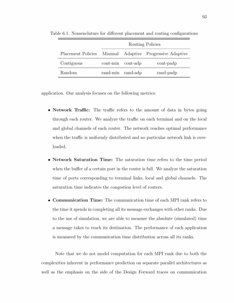
93

Table 6.1. Nomenclature for different placement and routing configurations

Routing Policies

Placement Policies Minimal Adaptive Progressive Adaptive

Contiguous cont-min cont-adp cont-padp

Random rand-min rand-adp rand-padp

application. Our analysis focuses on the following metrics:

• Network Traffic: The traffic refers to the amount of data in bytes going

through each router. We analyze the traffic on each terminal and on the local

and global channels of each router. The network reaches optimal performance

when the traffic is uniformly distributed and no particular network link is over-

loaded.

• Network Saturation Time: The saturation time refers to the time period

when the buffer of a certain port in the router is full. We analyze the saturation

time of ports corresponding to terminal links, local and global channels. The

saturation time indicates the congestion level of routers.

• Communication Time: The communication time of each MPI rank refers to

the time it spends in completing all its message exchanges with other ranks. Due

to the use of simulation, we are able to measure the absolute (simulated) time

a message takes to reach its destination. The performance of each application

is measured by the communication time distribution across all its ranks.

Note that we do not model computation for each MPI rank due to both the

complexities inherent in performance prediction on separate parallel architectures as

well as the emphasis on the side of the Design Forward traces on communication

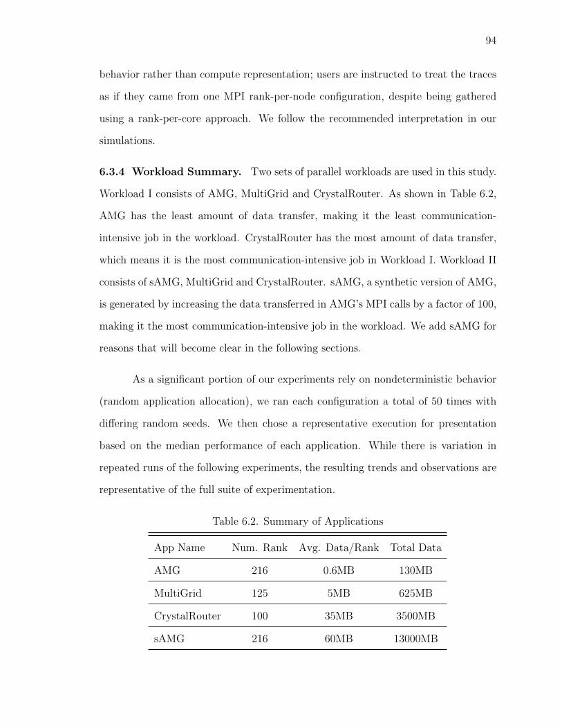
94

behavior rather than compute representation; users are instructed to treat the traces

as if they came from one MPI rank-per-node configuration, despite being gathered

using a rank-per-core approach. We follow the recommended interpretation in our

simulations.

6.3.4 Workload Summary. Two sets of parallel workloads are used in this study.

Workload I consists of AMG, MultiGrid and CrystalRouter. As shown in Table 6.2,

AMG has the least amount of data transfer, making it the least communication-

intensive job in the workload. CrystalRouter has the most amount of data transfer,

which means it is the most communication-intensive job in Workload I. Workload II

consists of sAMG, MultiGrid and CrystalRouter. sAMG, a synthetic version of AMG,

is generated by increasing the data transferred in AMG’s MPI calls by a factor of 100,

making it the most communication-intensive job in the workload. We add sAMG for

reasons that will become clear in the following sections.

As a significant portion of our experiments rely on nondeterministic behavior

(random application allocation), we ran each configuration a total of 50 times with

differing random seeds. We then chose a representative execution for presentation

based on the median performance of each application. While there is variation in

repeated runs of the following experiments, the resulting trends and observations are

representative of the full suite of experimentation.

Table 6.2. Summary of Applications

App Name Num. Rank Avg. Data/Rank Total Data

AMG 216 0.6MB 130MB

MultiGrid 125 5MB 625MB

CrystalRouter 100 35MB 3500MB

sAMG 216 60MB 13000MB

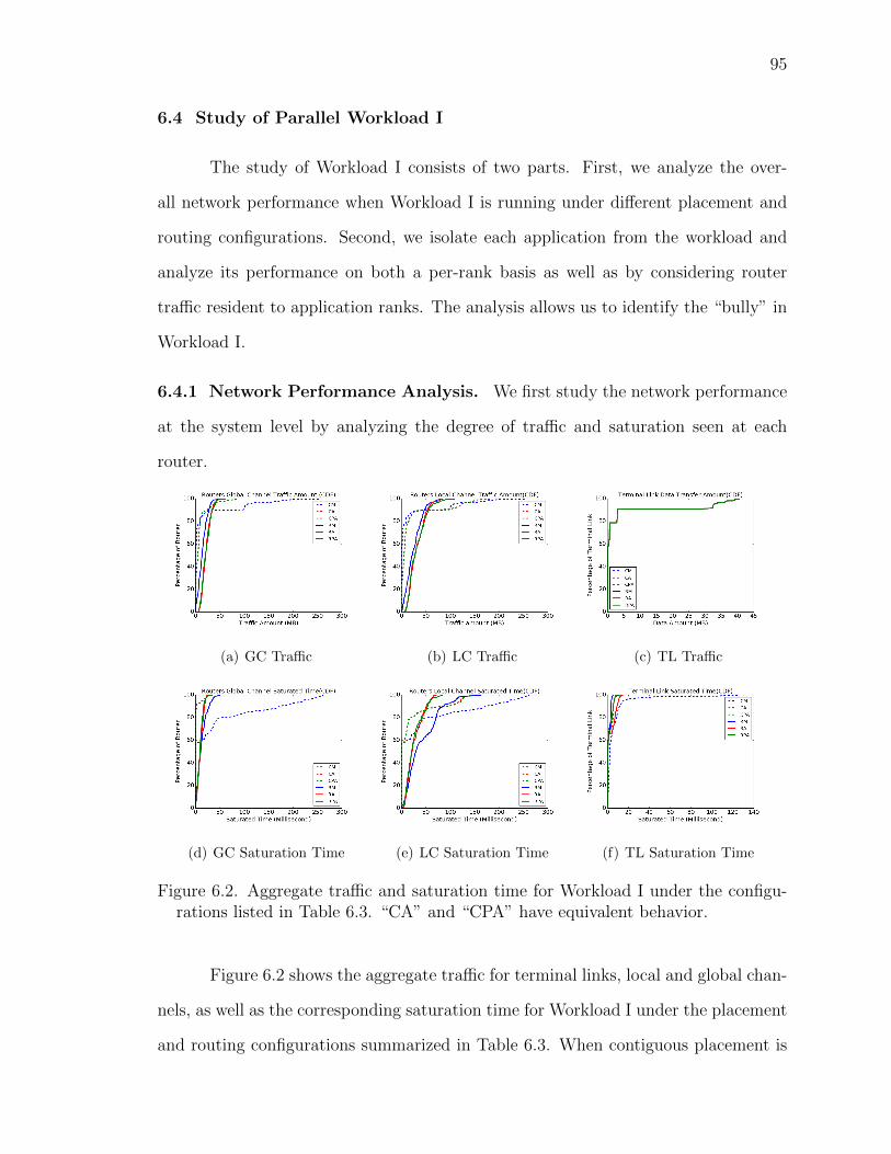
95

6.4 Study of Parallel Workload I

The study of Workload I consists of two parts. First, we analyze the over-

all network performance when Workload I is running under different placement and

routing configurations. Second, we isolate each application from the workload and

analyze its performance on both a per-rank basis as well as by considering router

traffic resident to application ranks. The analysis allows us to identify the “bully” in

Workload I.

6.4.1 Network Performance Analysis. We first study the network performance

at the system level by analyzing the degree of traffic and saturation seen at each

router.

(a) GC Traffic (b) LC Traffic (c) TL Traffic

(d) GC Saturation Time (e) LC Saturation Time (f) TL Saturation Time

Figure 6.2. Aggregate traffic and saturation time for Workload I under the configu-rations listed in Table 6.3. “CA” and “CPA” have equivalent behavior.

Figure 6.2 shows the aggregate traffic for terminal links, local and global chan-

nels, as well as the corresponding saturation time for Workload I under the placement

and routing configurations summarized in Table 6.3. When contiguous placement is

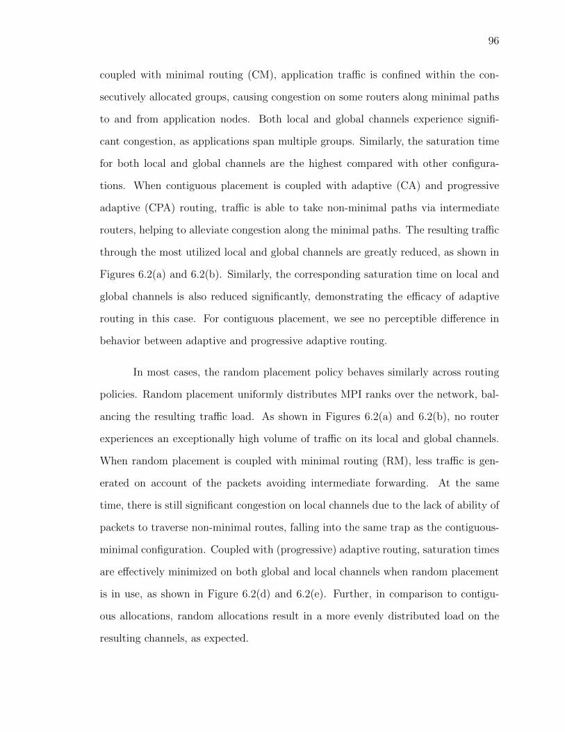
96

coupled with minimal routing (CM), application traffic is confined within the con-

secutively allocated groups, causing congestion on some routers along minimal paths

to and from application nodes. Both local and global channels experience signifi-

cant congestion, as applications span multiple groups. Similarly, the saturation time

for both local and global channels are the highest compared with other configura-

tions. When contiguous placement is coupled with adaptive (CA) and progressive

adaptive (CPA) routing, traffic is able to take non-minimal paths via intermediate

routers, helping to alleviate congestion along the minimal paths. The resulting traffic

through the most utilized local and global channels are greatly reduced, as shown in

Figures 6.2(a) and 6.2(b). Similarly, the corresponding saturation time on local and

global channels is also reduced significantly, demonstrating the efficacy of adaptive

routing in this case. For contiguous placement, we see no perceptible difference in

behavior between adaptive and progressive adaptive routing.

In most cases, the random placement policy behaves similarly across routing

policies. Random placement uniformly distributes MPI ranks over the network, bal-

ancing the resulting traffic load. As shown in Figures 6.2(a) and 6.2(b), no router

experiences an exceptionally high volume of traffic on its local and global channels.

When random placement is coupled with minimal routing (RM), less traffic is gen-

erated on account of the packets avoiding intermediate forwarding. At the same

time, there is still significant congestion on local channels due to the lack of ability of

packets to traverse non-minimal routes, falling into the same trap as the contiguous-

minimal configuration. Coupled with (progressive) adaptive routing, saturation times

are effectively minimized on both global and local channels when random placement

is in use, as shown in Figure 6.2(d) and 6.2(e). Further, in comparison to contigu-

ous allocations, random allocations result in a more evenly distributed load on the

resulting channels, as expected.

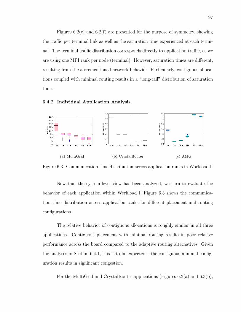
97

Figures 6.2(c) and 6.2(f) are presented for the purpose of symmetry, showing

the traffic per terminal link as well as the saturation time experienced at each termi-

nal. The terminal traffic distribution corresponds directly to application traffic, as we

are using one MPI rank per node (terminal). However, saturation times are different,

resulting from the aforementioned network behavior. Particularly, contiguous alloca-

tions coupled with minimal routing results in a “long-tail” distribution of saturation

time.

6.4.2 Individual Application Analysis.

(a) MultiGrid (b) CrystalRouter (c) AMG

Figure 6.3. Communication time distribution across application ranks in Workload I.

Now that the system-level view has been analyzed, we turn to evaluate the

behavior of each application within Workload I. Figure 6.3 shows the communica-

tion time distribution across application ranks for different placement and routing

configurations.

The relative behavior of contiguous allocations is roughly similar in all three

applications. Contiguous placement with minimal routing results in poor relative

performance across the board compared to the adaptive routing alternatives. Given

the analyses in Section 6.4.1, this is to be expected – the contiguous-minimal config-

uration results in significant congestion.

For the MultiGrid and CrystalRouter applications (Figures 6.3(a) and 6.3(b),

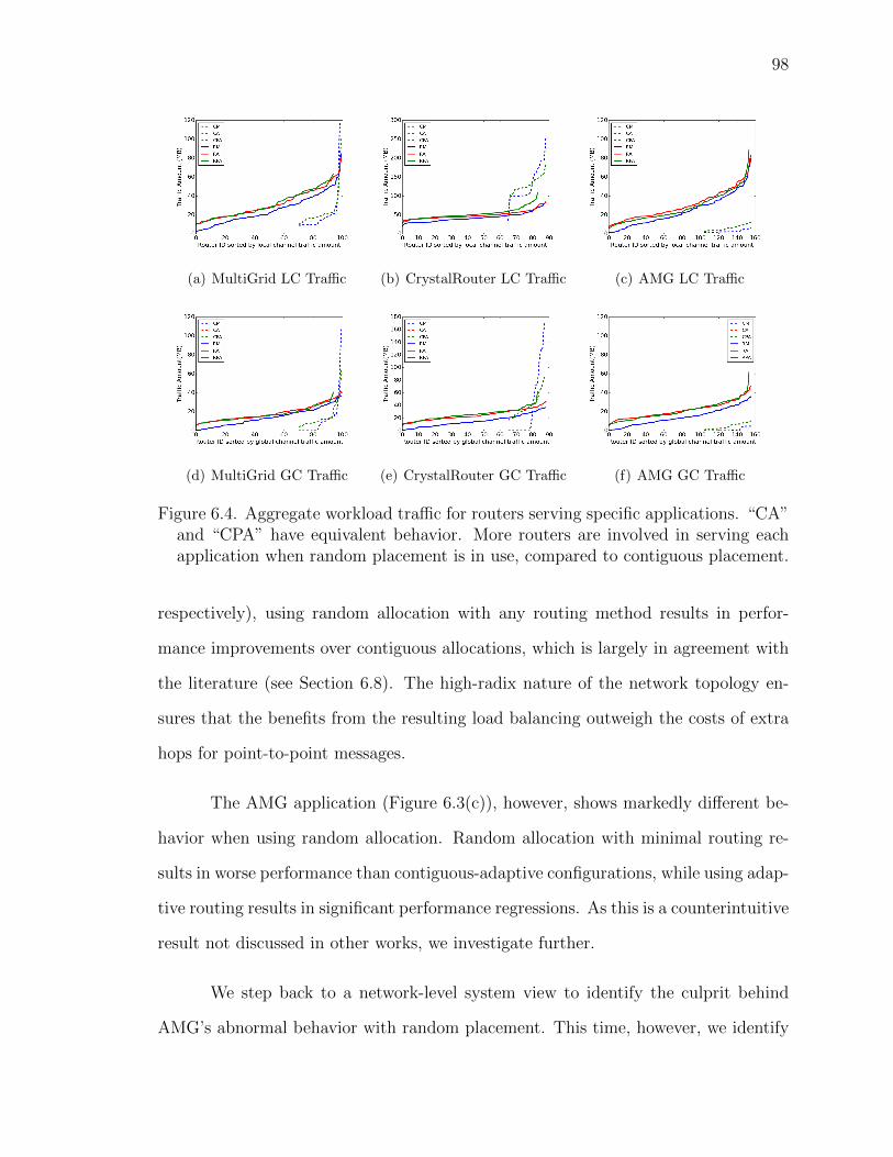
98

(a) MultiGrid LC Traffic (b) CrystalRouter LC Traffic (c) AMG LC Traffic

(d) MultiGrid GC Traffic (e) CrystalRouter GC Traffic (f) AMG GC Traffic

Figure 6.4. Aggregate workload traffic for routers serving specific applications. “CA”and “CPA” have equivalent behavior. More routers are involved in serving eachapplication when random placement is in use, compared to contiguous placement.

respectively), using random allocation with any routing method results in perfor-

mance improvements over contiguous allocations, which is largely in agreement with

the literature (see Section 6.8). The high-radix nature of the network topology en-

sures that the benefits from the resulting load balancing outweigh the costs of extra

hops for point-to-point messages.

The AMG application (Figure 6.3(c)), however, shows markedly different be-

havior when using random allocation. Random allocation with minimal routing re-

sults in worse performance than contiguous-adaptive configurations, while using adap-

tive routing results in significant performance regressions. As this is a counterintuitive

result not discussed in other works, we investigate further.

We step back to a network-level system view to identify the culprit behind

AMG’s abnormal behavior with random placement. This time, however, we identify

99

the compute nodes that each MPI rank resides on and the routers that are serving

each application, and analyze the traffic on a per-application basis. The results of this

experimentation are presented in Figure 6.4. Note that different numbers of routers

are used in the contiguous and random allocation configurations, as each router serves

multiple terminals.

The system behavior with respect to the CrystalRouter application arguably

best matches expectations. Use of contiguous allocations results in a subset of chan-

nels with a significant traffic load while a significant portion are unused. Use of ran-

dom allocations results in a comparatively smoother traffic distribution, with some

variation on the margins due to the randomness.

MultiGrid shows roughly similar behavior for contiguous allocations, but dif-

ferent behavior along the local channels. There is a significant variation in the traffic

distribution on local channels, even with adaptive routing, which nevertheless has the

net effect of reducing the maximal traffic load.

AMG shows a similar level of variation to MultiGrid in this case. However, it

is the least communication-intensive application of the three by a significant factor.

As evidenced by the wide gap between the router traffic in contiguous and random

placement configurations, the routers serving the AMG application are being utilized

by MultiGrid and CrystalRouter, resulting in AMG traffic contending with traffic of

other applications. The net effect, as shown in Figure 6.3(c), is significant slowdowns

for AMG. We refer to this phenomenon as AMG being “bullied” by MultiGrid and

CrystalRouter.

6.4.3 Key Observations. In summary, based on the simulations presented in

Section 6.4.1 and 6.4.2, we make the following observations.

System-level performance is significantly improved when random placement

100

and adaptive routing are in use. Random placement can uniformly distribute MPI

ranks of application over the network, and adaptive routing can redirect the traffic

from congested routers to other less busy routers. The combination of the two min-

imizes hot-spots and promotes load-balanced distribution. The resulting increased

number of hops per message was not a significant detriment in comparison. This

matches what is seen in the literature.

The performance of communication-intensive jobs in the system improves through

use of random allocation policies. Both CrystalRouter and MultiGrid, the two most

communication-intensive jobs, saw improved distributions of communication perfor-

mance when moving to a random allocation. Again, this matches what is seen in the

literature.

The performance of less communication-intensive jobs in workload regresses

when random placement and adaptive routing are in use. AMG in Workload I is “bul-

lied” by its concurrently running communication-intensive peers, MultiGrid and Crys-

talRouter. AMG shares routers and groups with MultiGrid and CrystalRouter under

random placement. The traffic from MultiGrid and CrystalRouter is (re)directed to

the routers that serve AMG, slowing down AMG’s communication. 3

In contrast, performance consistency of each application is achieved only when

contiguous placement and minimal routing are in use. As a corollary to the previ-

ous observation, router and group sharing among applications are guaranteed to be

prohibited when using contiguous placement with minimal routing (sharing of spare

nodes within a group notwithstanding). This renders the “bully” behavior moot,

though with the downside of significant performance degradation, so such approaches

3We have tried three different congestion “sensing” schemes in the literaturefor adaptive routing [96]. Although there are some variations between the results,none of the congestion sensing scheme prevent the “bully” behavior.

101

must be carefully considered.

6.5 Study of Parallel Workload II

In this section, we use a different experimental configuration to verify and

explore the observations made in the previous section. Specifically, we conduct the

same sets of experiments through Workload II, which consists of sAMG, MultiGrid

and CrystalRouter. By replacing AMG with sAMG, we turn the “bully” into the

“bullied”.

6.5.1 Network Performance Analysis. Figure 6.5 shows aggregate traffic and

saturation times for Workload II, corresponding to Figure 6.2 in Workload I. Replac-

ing AMG with sAMG results in greater aggregate traffic as well as more saturation

than in Workload I, but regardless, similar patterns can be observed. Contiguous

placement with minimal routing results in load imbalance with respect to both traffic

and saturation. The addition of adaptive routing alleviates these effects to some de-

gree, particularly with respect to global channel usage, while trading off saturation in

global channels for saturation in the local channels. Using random placement again

shows roughly similar performance characteristics across routing configurations, with

adaptive routing helping to balance aggregate load while increasing the aggregate

traffic due to the related indirection.

6.5.2 Individual Application Analysis. We study the performance of each

application individually in the same manner as in Section 6.4.2. Figure 6.6 shows the

communication time distributions of the ranks of the three applications, running con-

currently in Workload II. The “bully” in Workload I becomes the “bullied” in Work-

load II. MultiGrid and CrystalRouter are in this instance the less communication-

intensive applications. With random placement and (progressive) adaptive routing,

both MultiGrid and CrystalRouter experience prolonged communication time, as

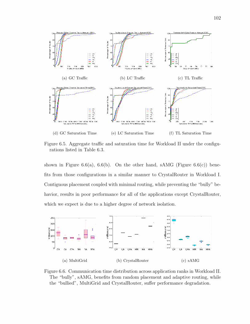
102

(a) GC Traffic (b) LC Traffic (c) TL Traffic

(d) GC Saturation Time (e) LC Saturation Time (f) TL Saturation Time

Figure 6.5. Aggregate traffic and saturation time for Workload II under the configu-rations listed in Table 6.3.

shown in Figure 6.6(a), 6.6(b). On the other hand, sAMG (Figure 6.6(c)) bene-

fits from those configurations in a similar manner to CrystalRouter in Workload I.

Contiguous placement coupled with minimal routing, while preventing the “bully” be-

havior, results in poor performance for all of the applications except CrystalRouter,

which we expect is due to a higher degree of network isolation.

(a) MultiGrid (b) CrystalRouter (c) sAMG

Figure 6.6. Communication time distribution across application ranks in Workload II.The “bully”, sAMG, benefits from random placement and adaptive routing, whilethe “bullied”, MultiGrid and CrystalRouter, suffer performance degradation.

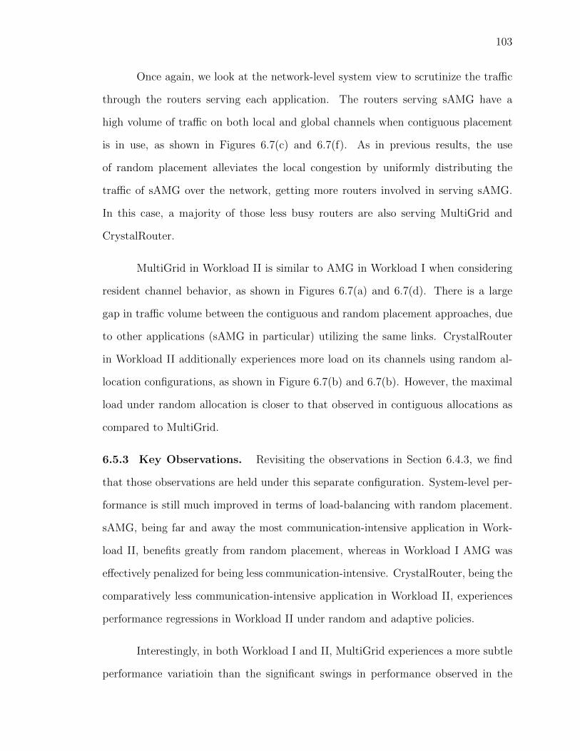
103

Once again, we look at the network-level system view to scrutinize the traffic

through the routers serving each application. The routers serving sAMG have a

high volume of traffic on both local and global channels when contiguous placement

is in use, as shown in Figures 6.7(c) and 6.7(f). As in previous results, the use

of random placement alleviates the local congestion by uniformly distributing the

traffic of sAMG over the network, getting more routers involved in serving sAMG.

In this case, a majority of those less busy routers are also serving MultiGrid and

CrystalRouter.

MultiGrid in Workload II is similar to AMG in Workload I when considering

resident channel behavior, as shown in Figures 6.7(a) and 6.7(d). There is a large

gap in traffic volume between the contiguous and random placement approaches, due

to other applications (sAMG in particular) utilizing the same links. CrystalRouter

in Workload II additionally experiences more load on its channels using random al-

location configurations, as shown in Figure 6.7(b) and 6.7(b). However, the maximal

load under random allocation is closer to that observed in contiguous allocations as

compared to MultiGrid.

6.5.3 Key Observations. Revisiting the observations in Section 6.4.3, we find

that those observations are held under this separate configuration. System-level per-

formance is still much improved in terms of load-balancing with random placement.

sAMG, being far and away the most communication-intensive application in Work-

load II, benefits greatly from random placement, whereas in Workload I AMG was

effectively penalized for being less communication-intensive. CrystalRouter, being the

comparatively less communication-intensive application in Workload II, experiences

performance regressions in Workload II under random and adaptive policies.

Interestingly, in both Workload I and II, MultiGrid experiences a more subtle

performance variatioin than the significant swings in performance observed in the

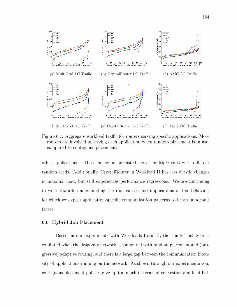
104

(a) MultiGrid LC Traffic (b) CrystalRouter LC Traffic (c) AMG LC Traffic

(d) MultiGrid GC Traffic (e) CrystalRouter GC Traffic (f) AMG GC Traffic

Figure 6.7. Aggregate workload traffic for routers serving specific applications. Morerouters are involved in serving each application when random placement is in use,compared to contiguous placement.

other applications. These behaviors persisted across multiple runs with different

random seeds. Additionally, CrystalRouter in Workload II has less drastic changes

in maximal load, but still experiences performance regressions. We are continuing

to work towards understanding the root causes and implications of this behavior,

for which we expect application-specific communication patterns to be an important

factor.

6.6 Hybrid Job Placement

Based on our experiments with Workloads I and II, the “bully” behavior is

exhibited when the dragonfly network is configured with random placement and (pro-

gressive) adaptive routing, and there is a large gap between the communication inten-

sity of applications running on the network. As shown through our experimentation,

contiguous placement policies give up too much in terms of congestion and load bal-

105

ance, hence being an impractical solution. Further, running each job with a dedicated

routing policy is unrealistic, since routing policy is part of system configuration which

can not be changed on the fly upon job submission.

As a natural extension of our observations, one question that arises is whether

we can combine the merits of random and contiguous placement policies in which each

application receives the performance benefits from system load balancing while avoiding

the “bully” behavior. As an initial exploration of the question, we set up a mock hybrid

job placement policy, in which less communication-intensive jobs receive contiguous

allocations to avoid the “bully” effect, while the communication-intensive jobs are

allocated randomly in order to distribute the communication load. For Workload I,

this means AMG gets a contiguous allocation while MultiGrid and CrystalRouter get

random allocations. Note that we do not consider challenges inherent in designing an

allocation policy for production usage, such as backfilling, reserving large contiguous

sets of nodes, determining a metric for communication intensity, etc., preferring a

restricted-scope experiment looking at the design space of dragonfly allocation policies

in light of our experimental observations.

(a) MultiGrid (b) CrystalRouter (c) sAMG

Figure 6.8. Application communication time. Workload I is running with all place-ment and routing configurations. Methods prefixed with “H” represent the hybridallocation approach.

For the purpose of brevity, we only present the communication time distribu-

tion of each application under all placement and routing configurations, including the

hybrid placement method. These results are presented in Figure 6.8. As shown in

106

Figure 6.8(a) and 6.8(b), MultiGrid and CrystalRouter exhibit similar performance in

both hybrid and random placement, as nodes are being placed randomly in each case.

While the performance of AMG under hybrid placement, shown in Figure 6.8(c), still

appears to exhibit significant communication interference on account of the other

applications as opposed to the best contiguous placement policies, the effects are sig-

nificantly reduced compared to a random-adaptive policy. We believe this to be a

result of more AMG-specific traffic occupying a smaller set of routers/groups, both

reducing the probability of traffic entering them through adaptive routing and in-

creasing the relative proportion of link utilization by AMG. Of course, this comes

with the costs associated with contiguous allocation, in which AMG’s traffic is less

likely to load balance across multiple dragonfly groups.

These initial experiments demonstrate some degree of benefit derived from us-

ing a hybrid approach, helping to alleviate the “bully” effect while retaining the per-

formance of communication-intensive applications. However, the behavior is still not

ideal in this case – AMG’s communications still experience performance degradation

versus the contiguous configurations. Hence, more work in this area is needed to fully

understand the intricate relationships between job scheduling and system/application

communication behavior to achieve optimal network utilization and application per-

formance in high-radix networks.

6.7 Other Placement Policies

The fact that hybrid job placement can not eliminate the adversary effect of the

“bully” behavior motivates us to explore other job placement policies. Random Router

placement, which has been studied by Jain et al.[5], is one possible job placement

policy for future dragonfly connected systems. In the Random Router placement

policy, a router is identified as “idle” if all its attached nodes are available. Idle

routers are randomly picked over the network, and all the compute nodes attached

107

to each router are assigned to a single job exclusively. Thus, the allocation made

by Random Router placement policy can preserve the locality within each router.

Compared with the random placement we discussed in Section 6.2.3, Random Router

placement makes a trade-off between the extent of randomness and locality.

Random Partition job placement policy is another possible solution for future

dragonfly systems. The partition based job placement has been adopted on torus

connected HPC systems such as IBM Blue Gene/P and Blue Gene/Q machines to

accommodate their capability computing workload. It has been well studied by Zhou

and Yang et al.[10][28][9]. Similarly, a partition could be configured as a portion of a

group in a dragonfly network. For example, in our simulated dragonfly network, we

define a partition as half a group, which consists of four routers. Thus, each parti-

tion will consist of 16 compute nodes. The Random Partition job placement policy

will assign each job some randomly picked partitions. Random Partition placement

preserves more locality and renders less randomness compared with Random Router

placement.

Table 6.3. Three different random placement and routing configurations

Routing

Placement Minimal Adaptive Prog Adaptive

Random rand-min rand-adp rand-padp

RandomRouter randR-min randR-adp randR-padp

RandomPartition randP-min randP-adp randP-padp

6.7.1 Individual Application Analysis. We present the communication time

distribution of each application in Workload I under three different random place-

ment policies and routing configurations, including the random placement policy we

discussed in section 6.2.3. These results are presented in Figure 6.9.

108

rand-m

in

rand-a

dp

rand-p

adp

randP-min

randP-ad

p

randP-pa

dp

randR-min

randR-ad

p

randR-pa

dp0123456789

millisecond

MG_CommunicationTime

(a) MultiGrid

rand-m

in

rand-a

dp

rand-p

adp

randP-min

randP-ad

p

randP-pa

dp

randR-min

randR-ad

p

randR-pa

dp35

40

45

50

55

60

65

70

75

milliseco

nd

CR_CommunicationTime

(b) CrystalRouter

rand-m

in

rand-a

dp

rand-p

adp

randP-min

randP-ad

p

randP-pa

dp

randR-min

randR-ad

p

randR-pa

dp0.8

1.0

1.2

1.4

1.6

1.8

2.0

2.2

2.4

millisecond

AMG_CommunicationTime

(c) sAMG

Figure 6.9. Application communication time. Workload I is running with threedifferent random placement policies coupled with three routing configurations.

As we discussed in section 6.4, MultiGrid and CrystalRouter prefer random

placement for the reason that their traffic can be evenly distributed across the net-

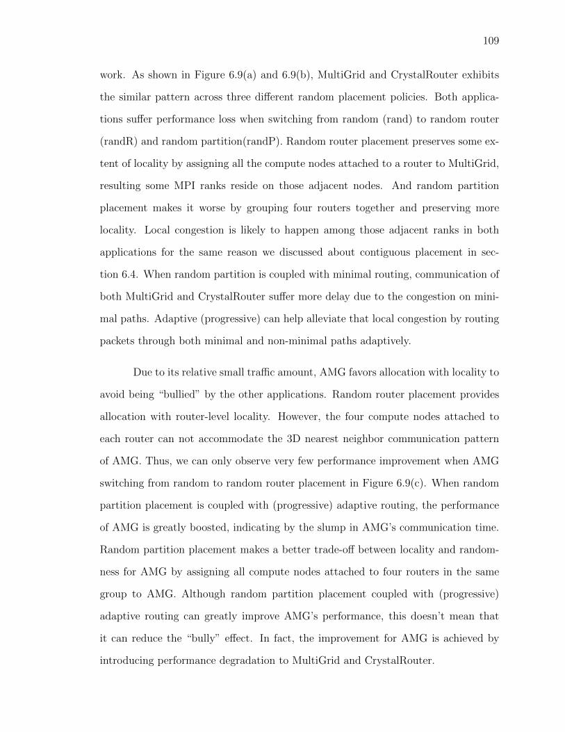
109

work. As shown in Figure 6.9(a) and 6.9(b), MultiGrid and CrystalRouter exhibits

the similar pattern across three different random placement policies. Both applica-

tions suffer performance loss when switching from random (rand) to random router

(randR) and random partition(randP). Random router placement preserves some ex-

tent of locality by assigning all the compute nodes attached to a router to MultiGrid,

resulting some MPI ranks reside on those adjacent nodes. And random partition

placement makes it worse by grouping four routers together and preserving more

locality. Local congestion is likely to happen among those adjacent ranks in both

applications for the same reason we discussed about contiguous placement in sec-

tion 6.4. When random partition is coupled with minimal routing, communication of

both MultiGrid and CrystalRouter suffer more delay due to the congestion on mini-

mal paths. Adaptive (progressive) can help alleviate that local congestion by routing

packets through both minimal and non-minimal paths adaptively.

Due to its relative small traffic amount, AMG favors allocation with locality to

avoid being “bullied” by the other applications. Random router placement provides

allocation with router-level locality. However, the four compute nodes attached to

each router can not accommodate the 3D nearest neighbor communication pattern

of AMG. Thus, we can only observe very few performance improvement when AMG

switching from random to random router placement in Figure 6.9(c). When random

partition placement is coupled with (progressive) adaptive routing, the performance

of AMG is greatly boosted, indicating by the slump in AMG’s communication time.

Random partition placement makes a better trade-off between locality and random-

ness for AMG by assigning all compute nodes attached to four routers in the same

group to AMG. Although random partition placement coupled with (progressive)

adaptive routing can greatly improve AMG’s performance, this doesn’t mean that

it can reduce the “bully” effect. In fact, the improvement for AMG is achieved by

introducing performance degradation to MultiGrid and CrystalRouter.

110

6.7.2 Key Observations. Based the experiments presented in section 6.7.1, we

can make the following observations.

Neither random router nor random partition placement can eliminate the “bully”

effect. Both placement policies can not avoid AMG sharing network with MultiGrid

and CrystalRouter, which is the root cause of “bully” effect. Traffic from each ap-

plication still need to share the local and global channel when traversing from the

source to the destination router.

MultiGrid and CrystalRouter prefer randomness over locality on dragonfly net-

work. Due to their high traffic volume, MultiGrid and CrystalRouter prefer random

placement to evenly distribute their traffic. Random router placement reduces the

randomness by preserving the router-level locality, introducing potential local conges-

tion and performance degradation to both applications. Random partition placement

makes it worse for MultiGrid and CrystalRouter as partition-level locality has been

preserved.

AMG benefits from allocation with high extent of locality. As the least commu-

nication intensive application in Workload I, AMG prefers exclusive network resource

without sharing with other applications. The locality preserved by random router

and random partition placement policy can reduce the sharing of routers between dif-

ferent applications. The performance of AMG can be greatly improved when random

partition placement is applied.

6.8 Related Work

The impact of job placement on system behavior and application performance

has been the subject of many studies. We focus on the HPC-centric studies here. Skin-

ner et al. identified significant performance variability due to network contention [108].

They found that performance variability is inevitable on either torus or fat-tree net-

111

works when network sharing among concurrently running applications is allowed.

Bhatele et al. studied the performance variability of a specific application, p3FD, run-

ning on different HPC production systems with torus network topologies [4]. They

obtained performance consistency in their application when network resources were

allocated compactly and exclusively and wide variability otherwise. Jokanovic et al.

studied the impact of job placement to the workload and claimed that the key to

reduce performance variability is to avoid network sharing [22].

Zhou et al. investigated the potential of relaxing network resource allocation

by utilizing application communication features[10]. They studied the performance of

a number of parallel benchmarks when assigning them with either mesh or torus con-

nected node allocation. Based on their observation, they proposed a communication-

aware scheduling policy that selectively allocates network resource to users jobs ac-

cording to job communication characteristics. Yang et al. proposed a window-based

locality-aware job scheduling design for HPC systems[28]. The objective of their

scheduling design is to preserve the locality with regard to node allocation, and in

the meanwhile maintain high system utilization. In another recent work from Yang

et al., they investigate the performance of applications with different communica-

tion characteristics when using different allocation and mapping strategies on torus

connected HPC systems [9].

Recently, several researchers have investigated job placement and routing al-

gorithms on dragonfly networks. Prisacari et al. proposed a communication-matrix-

based analytic modeling framework for mapping application workloads onto network

topologies [109]. They found that, in the context of dragonfly networks, optimizing

for throughput and not workload completion time is often misleading and the notion

of system balance cited as a dragonfly design parameter is not always directly appli-

cable to all workloads. Jain et al. conducted a comprehensive analysis of various job

112

placement and routing policies with regard to network link throughput on dragonfly

network [5]. Their work is based on an analytical model and synthetic workload.

Bhatele et al. used coarse-grain simulation to study the performance of synthetic

workloads under the different task mapping and routing policies on two-level direct

networks [6]. Mubarak et al. focused on the modeling of large-scale dragonfly networks

with parallel event driven simulation. The dragonfly network model for million-node

configurations presented in their work strongly scales when going from 1,024 to 65,536

MPI tasks on IBM Blue Gene/P and IBM Blue Gene/Q systems [102]. The dragonfly

model used in this paper is from their work.

Our work complements the literature in the following aspects. First, our

simulations are driven by real application traces intended to be representative of

production-scale application patterns. Second, we study a variety of different job

placement and routing policies that could be used on HPC systems with dragonfly

networks. This study could serve as an guideline for future system design and im-

plementation. Third, we holistically examine network behavior at both the overall

system level as well as the individual application level, though we do not consider

communication-pattern specific application mappings as Prisacari et al. did. Last but

not least, with the CODES simulation toolkit and related network models [102,110],

we are able to simulate and examine system and application behavior at a very fine

grain, collecting data at the dragonfly link level with packet-level fidelity. We believe

these differences allowed us to uncover the “bully” behavior, which to our knowledge

is unreported in the literature. However, in a sense, Prisacari et al.’s work suggests

these types of behaviors as possibilities deriving from the balance-first design rationale

for the dragonfly.

6.9 Summary

In this chapter, we have conducted extensive studies of system and application

113

behavior using various job placement and routing configurations on a dragonfly net-

work. We took a simulation-based approach, utilizing the CODES simulation toolkit

and related models for high-fidelity dragonfly simulation, driving the network with

three production-representative scientific application traces. We found that, under

the prevailing recommendation of random job placement and adaptive routing, net-

work traffic can be well distributed to achieve a balanced load and strong overall

performance, at the cost of impairing jobs with less intensive communication pat-

terns. We denoted this as the “bully” effect. On the other hand, contiguous process

placement prevents such effects while exacerbating local congestion, though this can

be mitigated through the addition of adaptive routing. Finally, we performed initial

experimentation exploring a mock “hybrid” contiguous/random job placement pol-

icy and two other random placement policies. Our preliminary study demonstrates

the need of specialized job placement strategy based on application communication

characteristics.

To the best of our knowledge, using real application traces from production

systems for the study of job interference on dragonfly networks has not been reported

in the literature so far. We believe the observations and new placement policy pre-

sented in this paper are valuable to the HPC community. We believe the observations

and new placement policy presented in this paper are valuable to a number of com-

munities including HPC computing facilities, system software developers, and system

administrators and HPC users. The computing facilities should take network resource

sharing into consideration when choosing proper configurations when building their

dragonfly networks. System software developers could design better scheduling algo-

rithms for jobs with distinct communication characteristics. System administrators

could make more accurate predication about system availability based on job running

status when system is configured with different placement and routing policies. Users

can provide detail information about their applications such that batch scheduler

114

could assign the optimal allocation to guarantee the quality of service.

115

CHAPTER 7

CONCLUSION

The batch scheduler plays an important role in managing and utilizing the

large scale HPC system. It serves as the interface between the users and the HPC

system, decides when and where to dispatch the submitted jobs for running on the

system. While the existing batch scheduling designs have been challenged by the

emerging issues in the exascale computing era, our research is motivated by exploring

the new scheduling algorithms and methodologies to solve those issues. The spe-

cific issues we identified to solve in our work include increasing energy cost, network

contention and job interference. In this dissertation, we have made the contribution

of addressing these issues in a orchestrated way by building a cooperative batching

scheduling framework that integrates novel batch scheduling algorithms and method-

ologies.

7.1 Summary of Contributions

We proposed new batch scheduling algorithms and methodologies, integrated

them in our new cooperative batch scheduling framework to address three major

challenges for HPC systems in exascale era. And we made following contributions:

• We propose an novel job power aware scheduling design, with the objective

to reduce the ever-increasing electricity bill for HPC systems. Our design is

based on the facts that HPC jobs have different individual power profiles and

that electricity prices vary throughout a day. By scheduling jobs with high

power profiles during low electricity pricing period and jobs with low power

profiles during high electricity pricing period, our scheduler is capable of cutting

the electricity bill of HPC systems by up to 23% without impacting system

utilization, which is critical to HPC systems.

116

• In order to balance performance with system performance, we design and im-

plement a window-based locality-aware job scheduling methodology for torus-

connected system. Being different from the traditional batch scheduler, our

design has three novel features. First, rather than one-by-one job scheduling,

our design takes a “window” of jobs (i.e.,multiple jobs) into consideration for

job prioritizing and resource allocation. Second, our design maintains a list of

slots to preserve node contiguity information for resource allocation. Finally, we

formulate a 0-1 Multiple Knapsack problem to describe our scheduling decision

making and present two algorithms to solve the problem. The comprehensive

trace-based simulations demonstrate our design can reduce average job wait

time by up to 28% and average job response time by 30%, with a slight im-

provement on overall system utilization.

• We study the communication behavior of three parallel applications: AMG,

Crystal Router, and MultiGrid on torus network with different placement poli-

cies and mapping strategies. We analyze the intra- and interjob interference

by simulating three applications running both independently and concurrently.

Based on our comprehensive experiments, we make some valuable observations

with regard to relation between application communication pattern and its per-

formance when different placement and mapping strategies are in use. We be-

lieve these observations can provide valuable guidance for HPC batch schedulers

and resource managers to make flexible job allocations. We claim that rather

than using predefined partitions or a noncontiguous placement policy, future

HPC systems should assign resources to each job based on job communication

patterns.

• We conduct extensive studies of system and application behavior using vari-

ous job placement and routing configurations on a dragonfly network. We find

117

that, under the prevailing recommendation of random job placement and adap-

tive routing, network traffic can be well distributed to achieve a balanced load

and strong overall performance, at the cost of impairing jobs with less intensive

communication patterns. We denoted this as the “bully” effect. On the other

hand, contiguous process placement prevents such effects while exacerbating

local congestion, though this can be mitigated through the addition of adaptive

routing. We explore a series of other possible job placement policies that can be

applied to dragonfly connected systems. Our study demonstrates the effective-

ness of specialized job placement strategy based on application communication

characteristics.

7.2 Future Research

A natural extension of our accomplished work is to enhance the cooperative

batch scheduling with deep understanding about application communication charac-

teristics, as well as new network topology.

7.2.1 Communication Characteristics. A thorough understanding about paral-

lel applications communication pattern is of great importance for the design of future

batch scheduling framework. However, communication pattern is a high level concept

regarding the communication characteristics of parallel applications. There are many

factors need to be considered to accurately analyze the communication pattern of

parallel application, such as communication topology (i.e., communication matrix),

intensity, frequency and operation dependence. We focus mainly on the study about

the communication topology and intensity of applications so far, however we believe

other factors, such as communication frequency, are also critical to the applications

communication performance when running on HPC systems. One possible direction

to continue the study about application communication pattern is to analyze the

communication frequency and its impact to the job placement policy.

118

7.2.2 Fat-tree Network Topology. Many HPC computing facilities will deploy

their next generation supercomputers with Fat-tree network topology. One of the

most prominent deployment of such system is the Summit supercomputer at Oak

Ridge National Laboratory [111]. The batch scheduler need to make topology-aware

job scheduling on the Fat-tree network. And the interference between jobs running

concurrently on Fat-tree network is also an open question. In order to design a

better batch scheduling for Fat-tree connected systems, lots of effort are required for

a comprehensive study on this topic.

119

BIBLIOGRAPHY

[1] M. Wright and al., The opportunities and challenges of exascale computing.http://science.energy.gov/, U.S. Department of Energy, 2010.

[2] X. Yang, Z. Zhou, S. Wallace, Z. Lan, W. Tang, S. Coghlan, and M. E. Papka,“Integrating dynamic pricing of electricity into energy aware scheduling for hpcsystems,” in Proceedings of the International Conference on High PerformanceComputing, Networking, Storage and Analysis, SC ’13, (New York, NY, USA),pp. 60:1–60:11, ACM, 2013.

[3] S. Wallace, V. Vishwanath, S. Coghlan, Z. Lan, and M. E. Papka, “Measuringpower consumption on ibm blue gene/q,” in Parallel and Distributed ProcessingSymposium Workshops PhD Forum (IPDPSW), 2013 IEEE 27th International,pp. 853–859, May 2013.

[4] A. Bhatele, K. Mohror, S. H. Langer, and K. E. Isaacs, “There goes the neigh-borhood: Performance degradation due to nearby jobs,” in Proceedings of theInternational Conference on High Performance Computing, Networking, Stor-age and Analysis, SC ’13, (New York, NY, USA), pp. 41:1–41:12, ACM, 2013.

[5] N. Jain, A. Bhatele, X. Ni, N. J. Wright, and L. V. Kale, “Maximizing through-put on a dragonfly network,” in Proceedings of the International Conference forHigh Performance Computing, Networking, Storage and Analysis, SC ’14, (Pis-cataway, NJ, USA), pp. 336–347, IEEE Press, 2014.

[6] A. Bhatele, W. D. Gropp, N. Jain, and L. V. Kale, “Avoiding hot-spots on two-level direct networks,” in High Performance Computing, Networking, Storageand Analysis (SC), 2011 International Conference for, pp. 1–11, Nov 2011.

[7] A. Bhatele, N. Jain, Y. Livnat, V. Pascucci, and P.-T. Bremer, “Analyzing net-work health and congestion in dragonfly-based supercomputers,” in Proceedingsof the IEEE International Parallel & Distributed Processing Symposium, IPDPS’16 (to appear), IEEE Computer Society, May 2016. LLNL-CONF-678293.

[8] X. Yang, J. Jenkins, M. Mubarak, R. B. Ross, and Z. Lan, “Watch out forthe bully!: Job interference study on dragonfly network,” in Proceedings ofthe International Conference for High Performance Computing, Networking,Storage and Analysis, SC ’16, (Piscataway, NJ, USA), pp. 64:1–64:11, IEEEPress, 2016.

[9] X. Yang, J. Jenkins, M. Mubarak, R. B. Ross, and Z. Lan, “Study of intra-and interjob interference on torus networks,” in 2016 IEEE 22nd InternationalConference on Parallel and Distributed Systems (ICPADS), pp. 239–246, Dec2016.

[10] Z. Zhou, X. Yang, Z. Lan, P. Rich, W. Tang, V. Morozov, and N. Desai, “Im-proving batch scheduling on blue gene/q by relaxing 5d torus network allocationconstraints,” in Parallel and Distributed Processing Symposium (IPDPS), 2015IEEE International, pp. 439–448, May 2015.

[11] Z. Zhou, X. Yang, Z. Lan, P. Rich, W. Tang, V. Morozov, and N. Desai, “Im-proving batch scheduling on blue gene/q by relaxing 5d torus network allocationconstraints,” IEEE Transactions on Parallel and Distributed Systems (To Ap-pear), 2016.

120

[12] Z. Zhou, X. Yang, D. Zhao, P. Rich, W. Tang, J. Wang, and Z. Lan, “I/o-aware batch scheduling for petascale computing systems,” in Cluster Computing(CLUSTER), 2015 IEEE International Conference on, pp. 254–263, Sept 2015.

[13] Z. Zhou, X. Yang, D. Zhao, P. Rich, W. Tang, J. Wang, and Z. Lan, “I/o-awarebandwidth allocation for petascale computing systems,” Parallel Computing.

[14] D. Zhao, X. Yang, I. Sadooghi, G. Garzoglio, S. Timm, and I. Raicu, “High-performance storage support for scientific applications on the cloud,” in Pro-ceedings of the 6th Workshop on Scientific Cloud Computing, ScienceCloud ’15,(New York, NY, USA), pp. 33–36, ACM, 2015.

[15] N. Liu, J. Cope, P. Carns, C. Carothers, R. Ross, G. Grider, A. Crume, andC. Maltzahn, “On the role of burst buffers in leadership-class storage systems,”in 2012 IEEE 28th Symposium on Mass Storage Systems and Technologies(MSST), pp. 1–11, April 2012.

[16] C. Patel, R. Sharma, C. Bash, and S. Graupner, “Energy aware grid: Globalworkload placement based on energy efficiency,” in ASME 2003 InternationalMechanical Engineering Congress and Exposition, pp. 267–275, American Soci-ety of Mechanical Engineers, 2003.

[17] S. Wallace, X. Yang, V. Vishwanath, W. E. Allcock, S. Coghlan, M. E. Papka,and Z. Lan, “A data driven scheduling approach for power management on hpcsystems,” in Proceedings of the International Conference for High PerformanceComputing, Networking, Storage and Analysis, SC ’16, (Piscataway, NJ, USA),pp. 56:1–56:11, IEEE Press, 2016.

[18] I. Redbooks, IBM System Blue Gene Solution: Blue Gene/Q System Adminis-tration. Vervante, 2012.

[19] C. Document, “Managing system software for cray xe and cray xt systems.,”2012.

[20] P. Krueger, T.-H. Lai, and V. A. Dixit-Radiya, “Job scheduling is more impor-tant than processor allocation for hypercube computers,” IEEE Transactionson Parallel and Distributed Systems, vol. 5, pp. 488–497, May 1994.

[21] J. A. Pascual, J. Navaridas, and J. Miguel-Alonso, “Job scheduling strate-gies for parallel processing,” ch. Effects of Topology-Aware Allocation Policieson Scheduling Performance, pp. 138–156, Berlin, Heidelberg: Springer-Verlag,2009.

[22] A. Jokanovic, J. Sancho, G. Rodriguez, A. Lucero, C. Minkenberg, andJ. Labarta, “Quiet neighborhoods: Key to protect job performance predictabil-ity,” in Parallel and Distributed Processing Symposium (IPDPS), 2015 IEEEInternational, pp. 449–459, May 2015.

[23] D. Chen, N. Eisley, P. Heidelberger, R. Senger, Y. Sugawara, S. Kumar, V. Sala-pura, D. Satterfield, B. Steinmacher-Burow, and J. Parker, “The ibm bluegene/q interconnection fabric,” IEEE Micro, vol. 32, pp. 32–43, Jan. 2012.

[24] Y. Ajima, T. Inoue, S. Hiramoto, Y. Takagi, and T. Shimizu, “The tofu inter-connect,” IEEE Micro, vol. 32, pp. 21–31, Jan. 2012.

[25] ORNL, “Titan system overview,” Accessed October 14, 2015. Available onlinehttps://www.olcf.ornl.gov/kbarticles/titan-system-overview.

121

[26] A. Gara, M. A. Blumrich, D. Chen, G.-T. Chiu, P. Coteus, M. E. Giampapa,R. A. Haring, P. Heidelberger, D. Hoenicke, G. V. Kopcsay, et al., “Overviewof the blue gene/l system architecture,” IBM Journal of Research and Devel-opment, vol. 49, no. 2.3, pp. 195–212, 2005.

[27] C. Albing, N. Troullier, S. Whalen, R. Olson, J. Glenski, H. Pritchard, andH. Mills, Scalable Node Allocation for Improved Performance in Regular andAnisotropic 3D Torus Supercomputers, pp. 61–70. Berlin, Heidelberg: SpringerBerlin Heidelberg, 2011.

[28] X. Yang, Z. Zhou, W. Tang, X. Zheng, J. Wang, and Z. Lan, “Balancing jobperformance with system performance via locality-aware scheduling on torus-connected systems,” in Cluster Computing (CLUSTER), 2014 IEEE Interna-tional Conference on, pp. 140–148, Sept 2014.

[29] M. Hennecke, W. Frings, W. Homberg, A. Zitz, M. Knobloch, and H. Bottiger,“Measuring power consumption on ibm blue gene/p,” Comput. Sci., vol. 27,pp. 329–336, Nov. 2012.

[30] A. Qureshi, R. Weber, H. Balakrishnan, J. Guttag, and B. Maggs, “Cutting theelectric bill for internet-scale systems,” in Proceedings of the ACM SIGCOMM2009 Conference on Data Communication, SIGCOMM ’09, (New York, NY,USA), pp. 123–134, ACM, 2009.

[31] DOE, “Design Forward - Exascale Initiative,” Accessed October 14, 2015. Avail-able online http://portal.nersc.gov/project/CAL/trace.htm.

[32] J. Cope, N. Liu, S. Lang, C. D. Carothers, and R. B. Ross, “Codes: Enabling co-design of multi-layer exascale storage architectures,” in Workshop on EmergingSupercomputing Technologies 2011 (WEST 2011), (Tuscon, AZ), 2011.

[33] Mira Supercomputer, “https://www.alcf.anl.gov/mira,” Accessed April 15,2017.

[34] TOP, “Top500 supercomputing web site,” Accessed October 14, 2015. Availableonline http://www.top500.org.

[35] J. Kim, W. Dally, S. Scott, and D. Abts, “Technology-driven, highly-scalabledragonfly topology,” in Computer Architecture, 2008. ISCA ’08. 35th Interna-tional Symposium on, pp. 77–88, June 2008.

[36] G. Faanes, A. Bataineh, D. Roweth, T. Court, E. Froese, B. Alverson, T. John-son, J. Kopnick, M. Higgins, and J. Reinhard, “Cray cascade: A scalable hpcsystem based on a dragonfly network,” in High Performance Computing, Net-working, Storage and Analysis (SC), 2012 International Conference for, pp. 1–9,Nov 2012.

[37] Moab, “http://www.adaptivecomputing.com/,” Accessed May 5, 2016.

[38] Portable Batch System, “http://www.pbsworks.com/,” Accessed May 5, 2016.

[39] Slurm Workload Manager by Schedmd, “http://slurm.schedmd.com/,” Ac-cessed May 5, 2016.

[40] Cobalt Resource Manager, “https://trac.mcs.anl.gov/projects/cobalt,” Ac-cessed May 5, 2016.

122

[41] “An event-driven simulator.” Available online http://bluesky.cs.iit.edu/cqsim.

[42] “Parallel workload archive.” Available online http://www.cs.huji.ac.il/labs/parallel/workload.

[43] P. C. Roth, J. S. Meredith, and J. S. Vetter, “Automated characterization ofparallel application communication patterns,” in Proceedings of the 24th Inter-national Symposium on High-Performance Parallel and Distributed Computing,HPDC ’15, (New York, NY, USA), pp. 73–84, ACM, 2015.

[44] S. S. Shende and A. D. Malony, “The tau parallel performance system,” Int. J.High Perform. Comput. Appl., vol. 20, pp. 287–311, May 2006.

[45] M. Michael, J. Curt, C. Mike, B. Jim, R. Philip, and M. Tushar, “mpiP:Lightweight, Scalable MPI profiling,” Accessed October 14, 2015. Availableonline at http://mpip.sourceforge.net.

[46] X. Wu, F. Mueller, and S. Pakin, “Automatic generation of executable com-munication specifications from parallel applications,” in Proceedings of the In-ternational Conference on Supercomputing, ICS ’11, (New York, NY, USA),pp. 12–21, ACM, 2011.

[47] SNL, “SST DUMPI trace library,” Accessed October 14, 2015. Available onlinehttp://sst.sandia.gov/usingdumpi.html.

[48] J. Vetter, S. Lee, D. Li, G. Marin, C. McCurdy, J. Meredith, P. Roth, andK. Spafford, “Quantifying architectural requirements of contemporary extreme-scale scientific applications,” in High Performance Computing Systems. Perfor-mance Modeling, Benchmarking and Simulation (S. A. Jarvis, S. A. Wright,and S. D. Hammond, eds.), vol. 8551 of Lecture Notes in Computer Science,pp. 3–24, Springer International Publishing, 2014.

[49] M. Mubarak, C. Carothers, R. Ross, and P. Carns, “Modeling a million-nodedragonfly network using massively parallel discrete-event simulation,” in HighPerformance Computing, Networking, Storage and Analysis (SCC), 2012 SCCompanion:, pp. 366–376, Nov 2012.

[50] P. D. Barnes, Jr., C. D. Carothers, D. R. Jefferson, and J. M. LaPre, “Warpspeed: Executing time warp on 1,966,080 cores,” in Proceedings of the 1st ACMSIGSIM Conference on Principles of Advanced Discrete Simulation, SIGSIMPADS ’13, (New York, NY, USA), pp. 327–336, ACM, 2013.

[51] W. Tang, Z. Lan, N. Desai, D. Buettner, and Y. Yu, “Reducing fragmentationon torus-connected supercomputers,” in Parallel Distributed Processing Sympo-sium (IPDPS), 2011 IEEE International, pp. 828–839, May 2011.

[52] C. Garcia-Martos, J. Rodriguez, and M. J. Sanchez, “Forecasting electricityprices by extracting dynamic common factors: application to the iberian mar-ket,” IET Generation, Transmission Distribution, vol. 6, pp. 11–20, January2012.

[53] J. Lundgren, J. Hellstrom, and N. Rudholm, “Multinational electricity marketintegration and electricity price dynamics,” in 2008 5th International Confer-ence on the European Electricity Market, pp. 1–6, May 2008.

123

[54] T. Ida, K. Ito, and M. Tanaka, “Using dynamic electricity pricing to addressenergy crises: Evidence from randomized field experiments,” 2013.

[55] L. A. Barroso and U. Hlzle, “The case for energy-proportional computing,”Computer, vol. 40, pp. 33–37, Dec 2007.

[56] P. Li, “Variational analysis of large power grids by exploring statistical sam-pling sharing and spatial locality,” in ICCAD-2005. IEEE/ACM InternationalConference on Computer-Aided Design, 2005., pp. 645–651, Nov 2005.

[57] J. Hikita, A. Hirano, and H. Nakashima, “Saving 200kw and $200 k/year bypower-aware job/machine scheduling,” in Parallel and Distributed Processing,2008. IPDPS 2008. IEEE International Symposium on, pp. 1–8, April 2008.

[58] Z. Cao, L. T. Watson, K. W. Cameron, and R. Ge, “A power aware studyfor vtdirect95 using dvfs,” in Proceedings of the 2009 Spring Simulation Multi-conference, SpringSim ’09, (San Diego, CA, USA), pp. 107:1–107:6, Society forComputer Simulation International, 2009.

[59] E. Pinheiro, R. Bianchini, E. V. Carrera, and T. Heath, “Load balancing andunbalancing for power and performance in cluster-based systems,” 2001.

[60] Y. Liu and H. Zhu, “A survey of the research on power management techniquesfor high-performance systems,” Softw. Pract. Exper., vol. 40, pp. 943–964, Oct.2010.

[61] M. Etinski, J. Corbalan, J. Labarta, and M. Valero, “Parallel job scheduling forpower constrained hpc systems,” Parallel Comput., vol. 38, pp. 615–630, Dec.2012.

[62] E. K. Lee, I. Kulkarni, D. Pompili, and M. Parashar, “Proactive thermal man-agement in green datacenters,” J. Supercomput., vol. 60, pp. 165–195, May2012.

[63] X. Fan, W.-D. Weber, and L. A. Barroso, “Power provisioning for a warehouse-sized computer,” in Proceedings of the 34th Annual International Symposiumon Computer Architecture, ISCA ’07, (New York, NY, USA), pp. 13–23, ACM,2007.

[64] C. Lefurgy, X. Wang, and M. Ware, “Power capping: A prelude to powershifting,” Cluster Computing, vol. 11, pp. 183–195, June 2008.

[65] Z. Zhou, Z. Lan, W. Tang, and N. Desai, Reducing Energy Costs for IBMBlue Gene/P via Power-Aware Job Scheduling, pp. 96–115. Berlin, Heidelberg:Springer Berlin Heidelberg, 2014.

[66] W. Tang, N. Desai, D. Buettner, and Z. Lan, “Analyzing and adjusting userruntime estimates to improve job scheduling on the blue gene/p,” in Paral-lel Distributed Processing (IPDPS), 2010 IEEE International Symposium on,pp. 1–11, April 2010.

[67] D. G. Feitelson and A. M. Weil, “Utilization and predictability in scheduling theibm sp2 with backfilling,” in Parallel Processing Symposium, 1998. IPPS/SPDP1998. Proceedings of the First Merged International ... and Symposium on Par-allel and Distributed Processing 1998, pp. 542–546, Mar 1998.

124

[68] J. M. Brandt, A. C. Gentile, D. J. Hale, and P. P. Pebay, “Ovis: a tool for intelli-gent, real-time monitoring of computational clusters,” in Proceedings 20th IEEEInternational Parallel Distributed Processing Symposium, pp. 8 pp.–, April 2006.

[69] T. H. Cormen, C. Stein, R. L. Rivest, and C. E. Leiserson, Introduction toAlgorithms. McGraw-Hill Higher Education, 2nd ed., 2001.

[70] W. Tang, N. Desai, D. Buettner, and Z. Lan, “Job scheduling with adjustedruntime estimates on production supercomputers,” Journal of Parallel and Dis-tributed Computing, vol. 73, no. 7, pp. 926 – 938, 2013. Best Papers: Interna-tional Parallel and Distributed Processing Symposium (IPDPS) 2010, 2011 and2012.

[71] Z. Zheng, L. Yu, W. Tang, Z. Lan, R. Gupta, N. Desai, S. Coghlan, and D. Buet-tner, “Co-analysis of ras log and job log on blue gene/p,” in Parallel DistributedProcessing Symposium (IPDPS), 2011 IEEE International, pp. 840–851, May2011.

[72] D. Tsafrir, K. Ouaknine, and D. G. Feitelson, “Reducing performance evalu-ation sensitivity and variability by input shaking,” in 2007 15th InternationalSymposium on Modeling, Analysis, and Simulation of Computer and Telecom-munication Systems, pp. 231–237, Oct 2007.

[73] V. J. Leung, E. M. Arkin, M. Bender, D. Bunde, J. Johnston, A. Lal, J. S. B.Mitchell, C. Phillips, and S. S. Seiden, “Processor allocation on cplant: achiev-ing general processor locality using one-dimensional allocation strategies,” inCluster Computing, 2002. Proceedings. 2002 IEEE International Conferenceon, pp. 296–304, 2002.

[74] X. Yang, Z. Zhou, S. Wallace, Z. Lan, W. Tang, S. Coghlan, and M. E. Papka,“Integrating dynamic pricing of electricity into energy aware scheduling for hpcsystems,” in Proceedings of the International Conference on High PerformanceComputing, Networking, Storage and Analysis, SC ’13, (New York, NY, USA),pp. 60:1–60:11, ACM, 2013.

[75] V. Lo, K. J. Windisch, W. Liu, and B. Nitzberg, “Noncontiguous processor al-location algorithms for mesh-connected multicomputers,” IEEE Trans. ParallelDistrib. Syst., vol. 8, pp. 712–726, July 1997.

[76] M. R. Garey and D. S. Johnson, Computers and Intractability: A Guide to theTheory of NP-Completeness. New York, NY, USA: W. H. Freeman & Co., 1979.

[77] D. Johnson, Near-optimal Bin Packing Algorithms. Massachusetts Institute ofTechnology, project MAC, Massachusetts Institute of Technology, 1973.

[78] D. S. Johnson, “Fast algorithms for bin packing,” Journal of Computer andSystem Sciences, vol. 8, no. 3, pp. 272–314, 1974.

[79] S. Martello and P. Toth, “Heuristic algorithms for the multiple knapsack prob-lem,” Computing, vol. 27, no. 2, pp. 93–112, 1981.

[80] A. Bhatele and L. V. Kale, “Application-specific topology-aware mapping forthree dimensional topologies,” in Parallel and Distributed Processing, 2008.IPDPS 2008. IEEE International Symposium on, pp. 1–8, April 2008.

125

[81] Department of Energy, “Characterization of the DOE Mini-apps,” AccessedApril 2, 2016. Available online http://portal.nersc.gov/project/CAL/designforward.htm.

[82] V. E. Henson and U. M. Yang, “Boomeramg: A parallel algebraic multigridsolver and preconditioner,” Applied Numerical Mathematics, vol. 41, no. 1,pp. 155 – 177, 2002. Developments and Trends in Iterative Methods for LargeSystems of Equations - in memorium Rudiger Weiss.

[83] R. E. Alcouffe, R. S. Baker, J. A. Dahl, S. A. Turner, and R. Ward, “PARTISN:A time-dependent, parallel neutral particle transport code system,” Los AlamosNational Laboratory, LA-UR-05-3925 (May 2005), 2005.

[84] Z. Joe and B. Randal, “SNAP: SN (Discrete Ordinates) Application Proxy,”Accessed October 14, 2015. Available online https://github.com/losalamos/SNAP.

[85] P. Fischer, A. Obabko, E. Merzari, and O. Marin, “Nek5000: Computationalfluid dynamics code,” Accessed October 14, 2015. Available online http://nek5000.mcs.anl.gov.

[86] J. Bell, A. Almgren, V. Beckner, M. Day, M. Lijewski, A. Nonaka, andW. Zhang, “Boxlib users guide,” tech. rep., Technical Report, CCSE,Lawrence Berkeley National Laboratory. Available at: https://ccse. lbl.gov/BoxLib/BoxLibUsersGuide. pdf, 2012.

[87] R. Fiedler and W. Stephen, “Improving task placement for applications with2d, 3d, and 4d virtual cartesian topologies on 3d torus networks with servicenodes,” in Proceedings of Cray User Group, 2013.

[88] Z. Zhou, X. Yang, Z. Lan, P. Rich, W. Tang, V. Morozov, and N. Desai, “Im-proving batch scheduling on blue gene/q by relaxing 5d torus network allocationconstraints,” in Parallel and Distributed Processing Symposium (IPDPS), 2015IEEE International, pp. 439–448, May 2015.

[89] D. Skinner and W. Kramer, “Understanding the causes of performance variabil-ity in hpc workloads,” in Workload Characterization Symposium, 2005. Proceed-ings of the IEEE International, pp. 137–149, Oct 2005.

[90] CORAL, “Collaboration benchmark codes,” Accessed October 14, 2015. Avail-able online https://asc.llnl.gov/CORAL-benchmarks.

[91] T. Hoefler, W. Gropp, W. Kramer, and M. Snir, “Performance modeling forsystematic performance tuning,” in High Performance Computing, Networking,Storage and Analysis (SC), 2011 International Conference for, pp. 1–12, Nov2011.

[92] B. Prisacari, G. Rodriguez, P. Heidelberger, D. Chen, C. Minkenberg, andT. Hoefler, “Efficient task placement and routing of nearest neighbor exchangesin dragonfly networks,” in Proceedings of the 23rd International Symposium onHigh-performance Parallel and Distributed Computing, HPDC ’14, (New York,NY, USA), pp. 129–140, ACM, 2014.

[93] D. Chen, N. Eisley, P. Heidelberger, R. Senger, Y. Sugawara, S. Kumar, V. Sala-pura, D. Satterfield, B. Steinmacher-Burow, and J. Parker, “The ibm blue

126

gene/q interconnection network and message unit,” in High Performance Com-puting, Networking, Storage and Analysis (SC), 2011 International Conferencefor, pp. 1–10, Nov 2011.

[94] J. Kim, W. Dally, S. Scott, and D. Abts, “Cost-efficient dragonfly topology forlarge-scale systems,” IEEE Micro, vol. 29, pp. 33–40, Jan. 2009.

[95] N. Jiang, J. Kim, and W. J. Dally, “Indirect adaptive routing on large scale in-terconnection networks,” in Proceedings of the 36th Annual International Sym-posium on Computer Architecture, ISCA ’09, (New York, NY, USA), pp. 220–231, ACM, 2009.

[96] J. Won, G. Kim, J. Kim, T. Jiang, M. Parker, and S. Scott, “Overcomingfar-end congestion in large-scale networks,” in High Performance ComputerArchitecture (HPCA), 2015 IEEE 21st International Symposium on, pp. 415–427, IEEE, 2015.

[97] D. Tsafrir, Y. Etsion, and D. G. Feitelson, “Backfilling using system-generatedpredictions rather than user runtime estimates,” IEEE Transactions on Paralleland Distributed Systems, vol. 18, pp. 789–803, June 2007.

[98] A. Jokanovic, J. C. Sancho, G. Rodriguez, A. Lucero, C. Minkenberg, andJ. Labarta, “Quiet neighborhoods: Key to protect job performance predictabil-ity,” in Parallel and Distributed Processing Symposium (IPDPS), 2015 IEEEInternational, pp. 449–459, May 2015.

[99] M. Misbah, D. C. Christopher, B. R. Robert, and C. Philip, “Enabling par-allel simulation of large-scale hpc network systems,” in TRANSACTIONS ONPARALLEL AND DISTRIBUTED COMPUTING,, pp. VOL. X, NO. X, 2015,IEEE, 2015.

[100] C. D. Carothers, D. Bauer, and S. Pearce, “ROSS: A high-performance, low-memory, modular Time Warp system,” Journal of Parallel and DistributedComputing, vol. 62, pp. 1648–1669, Nov. 2002.

[101] P. D. Barnes, Jr., C. D. Carothers, D. R. Jefferson, and J. M. LaPre, “WarpSpeed: Executing Time Warp on 1,966,080 Cores,” in Proceedings of the1st ACM SIGSIM Conference on Principles of Advanced Discrete Simulation,SIGSIM PADS ’13, (New York, NY, USA), pp. 327–336, ACM, 2013.

[102] M. Mubarak, C. D. Carothers, R. Ross, and P. Carns, “Modeling a million-nodedragonfly network using massively parallel discrete-event simulation,” in HighPerformance Computing, Networking, Storage and Analysis (SCC), 2012 SCCompanion:, pp. 366–376, Nov 2012.

[103] M. Mubarak, C. D. Carothers, R. B. Ross, and P. Carns, “A case study inusing massively parallel simulation for extreme-scale torus network codesign,”in Proceedings of the 2Nd ACM SIGSIM Conference on Principles of AdvancedDiscrete Simulation, SIGSIM PADS ’14, (New York, NY, USA), pp. 27–38,ACM, 2014.

[104] N. Liu and C. D. Carothers, “Modeling billion-node torus networks using mas-sively parallel discrete-event simulation,” in Proceedings of the 2011 IEEEWorkshop on Principles of Advanced and Distributed Simulation, PADS ’11,(Washington, DC, USA), pp. 1–8, IEEE Computer Society, 2011.

127

[105] N. Wolfe, C. Carothers, M. Mubarak, R. Ross, and P. Carns, “Modeling amillion-node slim fly network using parallel discrete-event simulation,” in Pro-ceedings of the 4Nd ACM SIGSIM Conference on Principles of Advanced Dis-crete Simulation, SIGSIM PADS ’16.

[106] N. Jiang, J. Balfour, D. U. Becker, B. Towles, W. J. Dally, G. Michelogiannakis,and J. Kim, “A detailed and flexible cycle-accurate network-on-chip simulator,”in Performance Analysis of Systems and Software (ISPASS), 2013 IEEE Inter-national Symposium on, pp. 86–96, April 2013.

[107] Department of Energy, “Exascale Initiative,” Accessed April 2, 2016. Availableonline http://www.exascaleinitiative.org/design-forward.

[108] D. Skinner and W. Kramer, “Understanding the causes of performance variabil-ity in hpc workloads,” in Workload Characterization Symposium, 2005. Proceed-ings of the IEEE International, pp. 137–149, Oct 2005.

[109] B. Prisacari, G. Rodriguez, P. Heidelberger, D. Chen, C. Minkenberg, andT. Hoefler, “Efficient task placement and routing of nearest neighbor exchangesin dragonfly networks,” in Proceedings of the 23rd International Symposium onHigh-performance Parallel and Distributed Computing, HPDC ’14, (New York,NY, USA), pp. 129–140, ACM, 2014.

[110] J. Cope, N. Liu, S. Lang, C. D. Carothers, and R. B. Ross, “Codes: Enabling co-design of multi-layer exascale storage architectures,” in Workshop on EmergingSupercomputing Technologies 2011 (WEST 2011), (Tuscon, AZ), 2011.

[111] Summit Supercomputer, “https://www.olcf.ornl.gov/summit/,” Accessed April15, 2017.

Documents

COOPERATIVE BATCH SCHEDULING FOR HPC SYSTEMS BY XU …mypages.iit.edu/~xyang56/papers/XuYang_Thesis_Final.pdf · 2017-05-26 · COOPERATIVE BATCH SCHEDULING FOR HPC SYSTEMS BY XU