Embed Size (px)
Citation preview

Integration of Scheduling and ControlOperations
Antonio Flores T.with colaborations from:
Sebastian Terrazas-Moreno, Miguel Angel Gutierrez-Limon, Ignacio E. Grossmann
Universidad Iberoamericana, Mexico
September 7, 2011
Antonio Flores T. with colaborations from: Sebastian Terrazas-Moreno, Miguel Angel Gutierrez-Limon, Ignacio E. Grossmann Universidad Iberoamericana, MexicoIntegration of Scheduling and Control Operations

Outline
I Introduction
I Aims of this talk
I Problem Definition
I Problem Assumptions
I Mixed-Integer Dynamic Optimization Approach
I Solving Mixed-Integer Dynamic Optimization Problems
I Single Stage Cycle Scheduling Formulation
I Full Discretization Optimal Control Formulation
I Simultaneous Scheduling and Control problems
I Single Stage Scheduling and Control Examples
I Parallel Lines Continuous Scheduling Problems
I MultiObjective Scheduling and Control Problems
I Conclusions
I Future Work
Antonio Flores T. with colaborations from: Sebastian Terrazas-Moreno, Miguel Angel Gutierrez-Limon, Ignacio E. Grossmann Universidad Iberoamericana, MexicoIntegration of Scheduling and Control Operations
Introduction
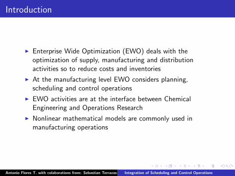
I Enterprise Wide Optimization (EWO) deals with theoptimization of supply, manufacturing and distributionactivities so to reduce costs and inventories
I At the manufacturing level EWO considers planning,scheduling and control operations
I EWO activities are at the interface between ChemicalEngineering and Operations Research
I Nonlinear mathematical models are commonly used inmanufacturing operations
Antonio Flores T. with colaborations from: Sebastian Terrazas-Moreno, Miguel Angel Gutierrez-Limon, Ignacio E. Grossmann Universidad Iberoamericana, MexicoIntegration of Scheduling and Control Operations
Introduction
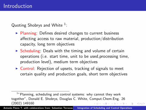
Quoting Shobrys and White 1:
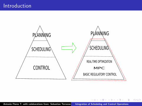
I Planning: Defines desired changes to current businessaffecting access to raw material, production/distributioncapacity, long term objectives
I Scheduling: Deals with the timing and volume of certainoperations (i.e. start time, unit to be used,processing time,production level), medium term objectives
I Control: Rejection of upsets, tracking of signals to meetcertain quality and production goals, short term objectives
1”Planning, scheduling and control systems: why cannot they worktogether”, Donald E. Shobrys, Douglas C. White, Comput.Chem.Eng. 26(2002) 149160
Antonio Flores T. with colaborations from: Sebastian Terrazas-Moreno, Miguel Angel Gutierrez-Limon, Ignacio E. Grossmann Universidad Iberoamericana, MexicoIntegration of Scheduling and Control Operations
Introduction
PLANNING
SCHEDULING
CONTROL
PLANNING
SCHEDULING
REAL-TIME OPTIMIZATION
MPC
BASIC REGULATORY CONTROL
Antonio Flores T. with colaborations from: Sebastian Terrazas-Moreno, Miguel Angel Gutierrez-Limon, Ignacio E. Grossmann Universidad Iberoamericana, MexicoIntegration of Scheduling and Control Operations

Introduction
I Two main approaches have been used for dealing withScheduling and Control problems
I The first one formulates the problem as a Mixed-IntegerDynamic Optimization (MIDO) problem
I MIDO problems can also incorporate logic decisions to switchamong different conditions
I The second one uses agents (i.e. heuristics) to model optimalsystem behavior
I Published SC problems include polymerization reactors, watertreatment plants, distillation columns and tubular reactors
Antonio Flores T. with colaborations from: Sebastian Terrazas-Moreno, Miguel Angel Gutierrez-Limon, Ignacio E. Grossmann Universidad Iberoamericana, MexicoIntegration of Scheduling and Control Operations

Aims of this Talk
In this work, we propose a simultaneous approach to address schedulingand control problems for a set of continuous plants. We take advantageof the rich knowledge of scheduling and optimal control formulations,and we merge them so the final result is a formulation able to solvesimultaneous scheduling and control problems.We cast the problem as an optimization problem. In the proposedformulation:
I Integer variables are used to determine the best production sequence
I Continuous variables take into account production times, cycle time,and inventories
Because dynamic profiles of both manipulated and controlled variablesare also decision variables, the resulting problem is cast as amixed-integer dynamic optimization (MIDO) problem.
Antonio Flores T. with colaborations from: Sebastian Terrazas-Moreno, Miguel Angel Gutierrez-Limon, Ignacio E. Grossmann Universidad Iberoamericana, MexicoIntegration of Scheduling and Control Operations
Problem Definition
Given are:
I A number of products to be manufactured in a single CSTR
I Lower bounds for the product demands
I Steady-state operating conditions for each desired product
I Cost of each product
I Inventory and raw materials costs
The problem consists in:
Simultaneous determination of a cyclic schedule (i.e. production wheel)and the control profile such that a given cost function is minimized
Major decisions involve:
I Selecting the cyclic time and Sequence in which the products will bemanufactured
I The transition times, Production rates, Length of processing times
I Amounts manufactured of each product
I Manipulated variables profiles for the transition
Antonio Flores T. with colaborations from: Sebastian Terrazas-Moreno, Miguel Angel Gutierrez-Limon, Ignacio E. Grossmann Universidad Iberoamericana, MexicoIntegration of Scheduling and Control Operations
Problem Assumptions
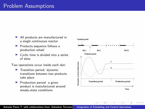
I All products are manufactured ina single continuous reactor
I Products sequence follows aproduction wheel
I Cyclic time is divided into a seriesof slots
Two operations occur inside each slot:
I Transition period: dynamictransitions between two productstake place
I Production period: a givenproduct is manufactured aroundsteady-state conditions
Production period
Slot 1 Slot 2 Slot Ns
Transition period
u
Time
Dyn
am
ic s
yst
em
beh
avio
ur
Production periodTransition period
x
Antonio Flores T. with colaborations from: Sebastian Terrazas-Moreno, Miguel Angel Gutierrez-Limon, Ignacio E. Grossmann Universidad Iberoamericana, MexicoIntegration of Scheduling and Control Operations
Mixed-Integer Dynamic Optimization Approach
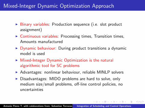
I Binary variables: Production sequence (i.e. slot productassignment)
I Continuous variables: Processing times, Transition times,Amounts manufactured
I Dynamic behaviour: During product transitions a dynamicmodel is used
I Mixed-Integer Dynamic Optimization is the naturalalgorithmic tool for SC problems
I Advantages: nonlinear behaviour, reliable MINLP solvers
I Disadvantages: MIDO problems are hard to solve, onlymedium size/small problems, off-line control policies, nouncertainties
Antonio Flores T. with colaborations from: Sebastian Terrazas-Moreno, Miguel Angel Gutierrez-Limon, Ignacio E. Grossmann Universidad Iberoamericana, MexicoIntegration of Scheduling and Control Operations
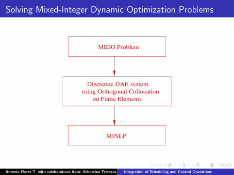
Solving Mixed-Integer Dynamic Optimization Problems
MIDO Problem
Discretize DAE system
using Orthogonal Collocation
on Finite Elements
MINLP
Antonio Flores T. with colaborations from: Sebastian Terrazas-Moreno, Miguel Angel Gutierrez-Limon, Ignacio E. Grossmann Universidad Iberoamericana, MexicoIntegration of Scheduling and Control Operations

Solving Mixed-Integer Dynamic Optimization Problems
I For solving Scheduling and Control problems we will show firsthow to handle the solution of Scheduling problems and afterthe numerical solution of dynamic optimization problems willbe addressed
I Scheduling: single stage and multiple stages
I Control: lumped and distributed parameters system
I Other MIDO solution approaches proposed
Antonio Flores T. with colaborations from: Sebastian Terrazas-Moreno, Miguel Angel Gutierrez-Limon, Ignacio E. Grossmann Universidad Iberoamericana, MexicoIntegration of Scheduling and Control Operations
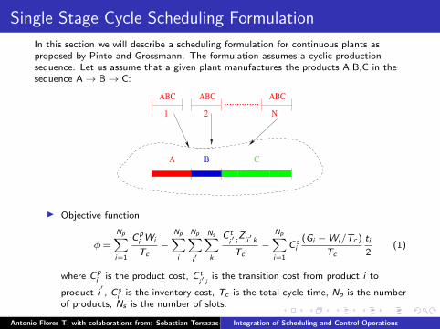
Single Stage Cycle Scheduling Formulation
In this section we will describe a scheduling formulation for continuous plants asproposed by Pinto and Grossmann. The formulation assumes a cyclic productionsequence. Let us assume that a given plant manufactures the products A,B,C in thesequence A→ B→ C:
ABC ABC ABC
1 2 N
A B C
..............
I Objective function
φ =
Np∑i=1
C pi Wi
Tc−
Np∑i
Np∑i′
Ns∑k
C ti′
iZ
ii′
k
Tc−
Np∑i=1
C si
(Gi −Wi/Tc )
Tc
ti
2(1)
where C pi is the product cost, C t
i′
iis the transition cost from product i to
product i′, C s
i is the inventory cost, Tc is the total cycle time, Np is the numberof products, Ns is the number of slots.
Antonio Flores T. with colaborations from: Sebastian Terrazas-Moreno, Miguel Angel Gutierrez-Limon, Ignacio E. Grossmann Universidad Iberoamericana, MexicoIntegration of Scheduling and Control Operations
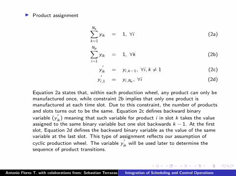
I Product assignment
Ns∑k=1
yik = 1, ∀i (2a)
Np∑i=1
yik = 1, ∀k (2b)
y′ik = yi,k−1, ∀i , k 6= 1 (2c)
y′i,1 = yi,Ns , ∀i (2d)
Equation 2a states that, within each production wheel, any product can only bemanufactured once, while constraint 2b implies that only one product ismanufactured at each time slot. Due to this constraint, the number of productsand slots turns out to be the same. Equation 2c defines backward binary
variable (y′ik ) meaning that such variable for product i in slot k takes the value
assigned to the same binary variable but one slot backwards k − 1. At the firstslot, Equation 2d defines the backward binary variable as the value of the samevariable at the last slot. This type of assignment reflects our assumption of
cyclic production wheel. The variable y′ik will be used later to determine the
sequence of product transitions.
Antonio Flores T. with colaborations from: Sebastian Terrazas-Moreno, Miguel Angel Gutierrez-Limon, Ignacio E. Grossmann Universidad Iberoamericana, MexicoIntegration of Scheduling and Control Operations
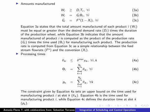
I Amounts manufactured
Wi ≥ Di Tc , ∀i (3a)
Wi = Gi Θi , ∀i (3b)
Gi = F o (1− Xi ), ∀i (3c)
Equation 3a states that the total amount manufactured of each product i (Wi )must be equal or greater than the desired demand rate (Di ) times the durationof the production wheel, while Equation 3b indicates that the amountmanufactured of product i is computed as the product of the production rate(Gi ) times the time used (Θi ) for manufacturing such product. The productionrate is computed from Equation 3c as a simple relationship between the feedstream flowrate (F o ) and the conversion (Xi ).
I Processing times
θik ≤ θmax yik , ∀i , k (4a)
Θi =
Ns∑k=1
θik , ∀i (4b)
pk =
Np∑i=1
θik , ∀k (4c)
The constraint given by Equation 4a sets an upper bound on the time used formanufacturing product i at slot k (θik ). Equation 4b is the time used formanufacturing product i , while Equation 4c defines the duration time at slot k(pk ).
Antonio Flores T. with colaborations from: Sebastian Terrazas-Moreno, Miguel Angel Gutierrez-Limon, Ignacio E. Grossmann Universidad Iberoamericana, MexicoIntegration of Scheduling and Control Operations

I Transitions between products
zipk ≥ y′pk + yik − 1, ∀i, p, k (5)
The constraint given in Equation 5 is used for defining the binary production transition variable zipk . Ifsuch variable is equal to 1 then a dynamic transition will occur from product i to product p within slot k,zipk will be zero otherwise.
I Timing relations
θtk =
Np∑i=1
Np∑p=1
ttpi zipk , ∀k (6a)
ts1 = 0 (6b)
tek = ts
k + pk +
Np∑i=1
Np∑p=1
ttpi zipk , ∀k (6c)
tsk = te
k−1, ∀k 6= 1 (6d)
tek ≤ Tc , ∀k (6e)
tfck = (f − 1)θt
k
Nfe
+θt
k
Nfe
γc , ∀f , c, k (6f)
Equation 6a defines the transition time from product i to product p at slot k. It should be remarked that the termttpi stands only for an estimate of the expected transition times. Equation 6b sets to zero the time at the beginning
of the production wheel cycle corresponding to the first slot. Equation 6c is used for computing the time at the endof each slot as the sum of the slot start time plus the processing time and the transition time. Equation 6d statesthat the start time at all the slots, different than the first one, is just the end time of the previous slot. Equation 6eis used to force that the end time at each slot be less than the production wheel cyclic time. Finally, Equation 6f isused to obtain the time value inside each finite element and for each internal collocation point.
Antonio Flores T. with colaborations from: Sebastian Terrazas-Moreno, Miguel Angel Gutierrez-Limon, Ignacio E. Grossmann Universidad Iberoamericana, MexicoIntegration of Scheduling and Control Operations

Simple Single Line Scheduling Example
Let us assume that a given plant facility manufactures three products: A,B,C. We would like to compute theoptimal cyclic production sequence that maximizes the process profit while meeting the demand rate of eachproduct.
C
B
A
C
B
A
C
B
A
1 2 3
Transition times(Transition cost)
A B C
A10
(4000)20
(8000)
B15
(3500)30
(6000)
C10
(7000)25
(5500)
Process dataProduct Demand Price Process Inventory
rate Products rates costA 2.1 320 8 1.5B 3 430 9 1C 4 450 12 2
Optimal Cyclic Scheduling Results: Profit=329Slot Product Process Amount Start End
time Manufactured time time1 B 235.3 2117.7 0 265.32 A 185.3 1482.4 265.3 460.63 C 235.3 2823.5 460.6 705.9
Antonio Flores T. with colaborations from: Sebastian Terrazas-Moreno, Miguel Angel Gutierrez-Limon, Ignacio E. Grossmann Universidad Iberoamericana, MexicoIntegration of Scheduling and Control Operations

Full Discretization Optimal Control Formulation
DAE Optimization Variational Approach
Sequential Approach
Multiple Shooting Simultaneous Approach
Pontryagin
Inefficient for constrained problems
state variables
Discretize some
Handles instabilities
Large NLP
Discretize Controls
Small NLP
Can not handle instabilities properly
state variables
Discretize all
NLP problem
Efficient for constrained problems
Large NLP
Handles instabilities
Antonio Flores T. with colaborations from: Sebastian Terrazas-Moreno, Miguel Angel Gutierrez-Limon, Ignacio E. Grossmann Universidad Iberoamericana, MexicoIntegration of Scheduling and Control Operations
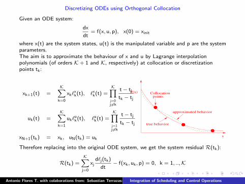
Discretizing ODEs using Orthogonal Collocation
Given an ODE system:
dx
dt= f(x, u, p), x(0) = xinit
where x(t) are the system states, u(t) is the manipulated variable and p are the systemparameters.The aim is to approximate the behaviour of x and u by Lagrange interpolationpolynomials (of orders K+ 1 and K, respectively) at collocation or discretizationpoints tk:
xk+1(t) =K∑
k=0
xk`xk(t), `x
k(t) =K∏
j=0j 6=k
t− tj
tk − tj
uk(t) =K∑
k=1
uk`uk(t), `u
k(t) =K∏
j=1j 6=k
t− tj
tk − tj
xN+1(tk) = xk, uN(tk) = uk
F(x)
x
Collocationpoints
true behavior
approximated behavior
Therefore replacing into the original ODE system, we get the system residual R(tk):
R(tk) =K∑
j=0
xjd`j(tk)
dt− f(xk, uk, p) = 0, k = 1, ..,K
Antonio Flores T. with colaborations from: Sebastian Terrazas-Moreno, Miguel Angel Gutierrez-Limon, Ignacio E. Grossmann Universidad Iberoamericana, MexicoIntegration of Scheduling and Control Operations
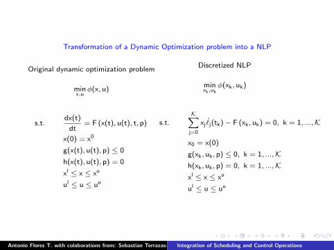
Transformation of a Dynamic Optimization problem into a NLP
Original dynamic optimization problem
minx,u
φ(x, u)
s.t.dx(t)
dt= F (x(t), u(t), t, p)
x(0) = x0
g(x(t), u(t), p) ≤ 0
h(x(t), u(t), p) = 0
xl ≤ x ≤ xu
ul ≤ u ≤ uu
Discretized NLP
minxk,uk
φ(xk, uk)
s.t.K∑
j=0
xj˙j(tk)− F (xk, uk) = 0, k = 1, ...,K
x0 = x(0)
g(xk, uk, p) ≤ 0, k = 1, ...,Kh(xk, uk, p) = 0, k = 1, ...,Kxl ≤ x ≤ xu
ul ≤ u ≤ uu
Antonio Flores T. with colaborations from: Sebastian Terrazas-Moreno, Miguel Angel Gutierrez-Limon, Ignacio E. Grossmann Universidad Iberoamericana, MexicoIntegration of Scheduling and Control Operations
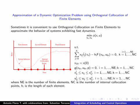
Approximation of a Dynamic Optimization Problem using Orthogonal Collocation ofFinite Elements
Sometimes it is convenient to use Orthogonal Collocation on Finite Elements toapproximate the behavior of systems exhibiting fast dynamics.
Sta
te
First element Second Element Third Element
Time
Points
CollocationInternal System behavior
minxk,uk
φ(x, u)
s.t.K∑
j=0
xij˙j(τk)− hiF (xik, uik) = 0,
i=1,...,NE
k = 1, ...,NC
x10 = x(0)
g(xik, uik, p) = 0, i = 1, ...,NE; k = 1, ..,NC
xlij ≤ xij ≤ xu
ij, i = 1, ...,NE; k = 1, ..,NC
ulij ≤ uij ≤ uu
ij, i = 1, ...,NE; k = 1, ..,NCwhere NE is the number of finite elements, NC is the number of internal collocationpoints, hi is the length of each element.
Antonio Flores T. with colaborations from: Sebastian Terrazas-Moreno, Miguel Angel Gutierrez-Limon, Ignacio E. Grossmann Universidad Iberoamericana, MexicoIntegration of Scheduling and Control Operations
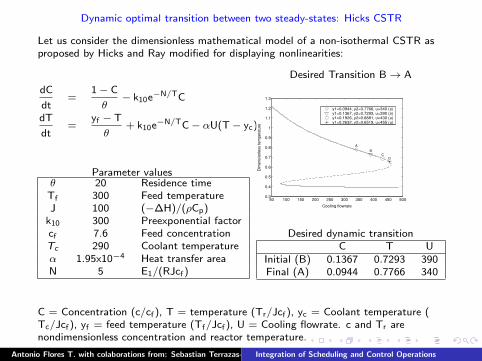
Dynamic optimal transition between two steady-states: Hicks CSTR
Let us consider the dimensionless mathematical model of a non-isothermal CSTR asproposed by Hicks and Ray modified for displaying nonlinearities:
dC
dt=
1− C
θ− k10e−N/TC
dT
dt=
yf − T
θ+ k10e−N/TC− αU(T− yc)
Parameter valuesθ 20 Residence time
Tf 300 Feed temperatureJ 100 (−∆H)/(ρCp)
k10 300 Preexponential factorcf 7.6 Feed concentrationTc 290 Coolant temperatureα 1.95x10⁻⁴ Heat transfer areaN 5 E1/(RJcf )
Desired Transition B→ A
50 100 150 200 250 300 350 400 450 5000.3
0.4
0.5
0.6
0.7
0.8
0.9
1
1.1
1.2
1.3
Cooling flowrate
Dim
en
sio
nle
ss t
em
pe
ratu
re
y1=0.0944, y2=0.7766, u=340 (s)y1=0.1367, y2=0.7293, u=390 (s)y1=0.1926, y2=0.6881, u=430 (u)y1=0.2632, y2=0.6519, u=455 (u)
A
B C
D
Desired dynamic transitionC T U
Initial (B) 0.1367 0.7293 390Final (A) 0.0944 0.7766 340
C = Concentration (c/cf ), T = temperature (Tr/Jcf ), yc = Coolant temperature (Tc/Jcf ), yf = feed temperature (Tf/Jcf ), U = Cooling flowrate. c and Tr arenondimensionless concentration and reactor temperature.
Antonio Flores T. with colaborations from: Sebastian Terrazas-Moreno, Miguel Angel Gutierrez-Limon, Ignacio E. Grossmann Universidad Iberoamericana, MexicoIntegration of Scheduling and Control Operations

Simultaneous approach for optimal control problems
I Objective functionAs objective function the requirement of minimum transition time between theinitial and final steady-states will be imposed:
Min
∫ tf
0
α1(C(t)− Cdes)2 + α2(T(t)− Tdes)2 + α3(U(t)− Udes)2
dt
the subscript ”des” stands for the final desired values. αi, i = 1, 2, 3 areweighting factors. The above integral is approximated using a Radau quadratureprocedure:
Min Φ =
Ne∑i=1
hi
Nc∑j=1
Wj
[α1(Cij − Cdes)2 + α2(Tij − Tdes)2 + α3(Uij − Udes)2
]Ne is the number of finite elements (Ne=3), Nc is the number of collocationpoints including the right boundary in each element (so in this case Nc = 3), Cij
and Tij are the dimensionless concentration and temperature values at eachdiscretized ij point, hi is the finite element length of the i−th element, Wj arethe Radau quadrature weights.
Antonio Flores T. with colaborations from: Sebastian Terrazas-Moreno, Miguel Angel Gutierrez-Limon, Ignacio E. Grossmann Universidad Iberoamericana, MexicoIntegration of Scheduling and Control Operations
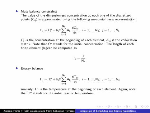
I Mass balance constraintsThe value of the dimensionless concentration at each one of the discretizedpoints (Cij) is approximated using the following monomial basis representation:
Cij = Coi + hiθ
Nc∑k=1
AkjdCik
dt, i = 1, ...,Ne; j = 1, ...,Nc
Coi is the concentration at the beginning of each element, Akj is the collocation
matrix. Note that Co1 stands for the initial concentration. The length of each
finite element (hi)can be computed as:
hi =1
Ne
I Energy balance
Tij = Toi + hiθ
Nc∑k=1
AkjdTik
dt, i = 1, ...,Ne; j = 1, ...,Nc
similarly, Toi is the temperature at the beginning of each element. Again, note
that To1 stands for the initial reactor temperature.
Antonio Flores T. with colaborations from: Sebastian Terrazas-Moreno, Miguel Angel Gutierrez-Limon, Ignacio E. Grossmann Universidad Iberoamericana, MexicoIntegration of Scheduling and Control Operations
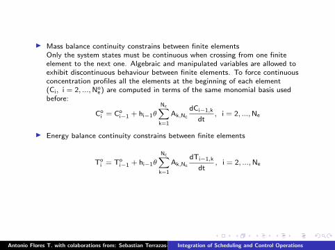
I Mass balance continuity constrains between finite elementsOnly the system states must be continuous when crossing from one finiteelement to the next one. Algebraic and manipulated variables are allowed toexhibit discontinuous behaviour between finite elements. To force continuousconcentration profiles all the elements at the beginning of each element(Ci, i = 2, ...,No
e) are computed in terms of the same monomial basis usedbefore:
Coi = Co
i−1 + hi−1θ
Nc∑k=1
Ak,Nc
dCi−1,k
dt, i = 2, ...,Ne
I Energy balance continuity constrains between finite elements
Toi = To
i−1 + hi−1θ
Nc∑k=1
Ak,Nc
dTi−1,k
dt, i = 2, ...,Ne
Antonio Flores T. with colaborations from: Sebastian Terrazas-Moreno, Miguel Angel Gutierrez-Limon, Ignacio E. Grossmann Universidad Iberoamericana, MexicoIntegration of Scheduling and Control Operations
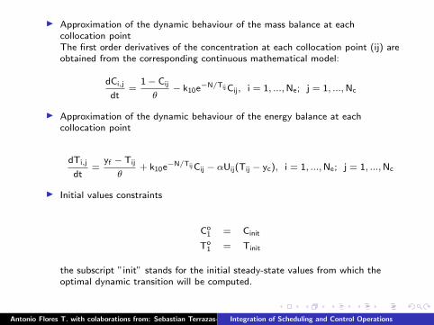
I Approximation of the dynamic behaviour of the mass balance at eachcollocation pointThe first order derivatives of the concentration at each collocation point (ij) areobtained from the corresponding continuous mathematical model:
dCi,j
dt=
1− Cij
θ− k10e−N/Tij Cij, i = 1, ...,Ne; j = 1, ...,Nc
I Approximation of the dynamic behaviour of the energy balance at eachcollocation point
dTi,j
dt=
yf − Tij
θ+ k10e−N/Tij Cij − αUij(Tij − yc), i = 1, ...,Ne; j = 1, ...,Nc
I Initial values constraints
Co1 = Cinit
To1 = Tinit
the subscript ”init” stands for the initial steady-state values from which theoptimal dynamic transition will be computed.
Antonio Flores T. with colaborations from: Sebastian Terrazas-Moreno, Miguel Angel Gutierrez-Limon, Ignacio E. Grossmann Universidad Iberoamericana, MexicoIntegration of Scheduling and Control Operations
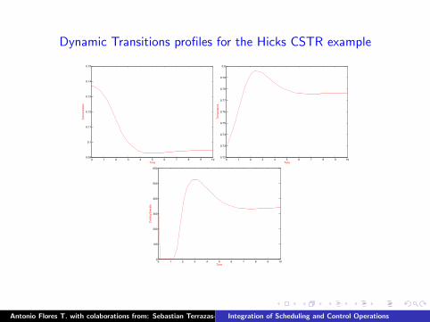
Dynamic Transitions profiles for the Hicks CSTR example
0 1 2 3 4 5 6 7 8 9 100.09
0.1
0.11
0.12
0.13
0.14
0.15
Time
Co
nce
ntr
atio
n
0 1 2 3 4 5 6 7 8 9 100.72
0.73
0.74
0.75
0.76
0.77
0.78
0.79
0.8
Time
Te
mp
era
ture
0 1 2 3 4 5 6 7 8 9 100
100
200
300
400
500
600
Time
Co
olin
g f
low
rate
Antonio Flores T. with colaborations from: Sebastian Terrazas-Moreno, Miguel Angel Gutierrez-Limon, Ignacio E. Grossmann Universidad Iberoamericana, MexicoIntegration of Scheduling and Control Operations
Simultaneous Scheduling and Control problems
I We have shown how to handle the solution of Scheduling andOptimal Control problems
I Because of strong interactions between Scheduling andControl Problems better optimal solutions can be found bythe simultaneous solution of these problems
I No need to neglect process dynamics (Scheduling)
I No need to fix production sequence (Control)
I Merge both formulations and solve MIDO problem
Antonio Flores T. with colaborations from: Sebastian Terrazas-Moreno, Miguel Angel Gutierrez-Limon, Ignacio E. Grossmann Universidad Iberoamericana, MexicoIntegration of Scheduling and Control Operations

Simultaneous Scheduling and Control problems
I Full discretization approaches lead to large size MINLPproblems
I Reliable MINLP solvers are needed
I Problem solution is highly-dependent on MINLP initializationscheme
I Use Scheduling and Control MINLP solutions for providingacceptable initial guesses of the decision variables
I Develop your Scheduling and Control formulation step by step
Antonio Flores T. with colaborations from: Sebastian Terrazas-Moreno, Miguel Angel Gutierrez-Limon, Ignacio E. Grossmann Universidad Iberoamericana, MexicoIntegration of Scheduling and Control Operations
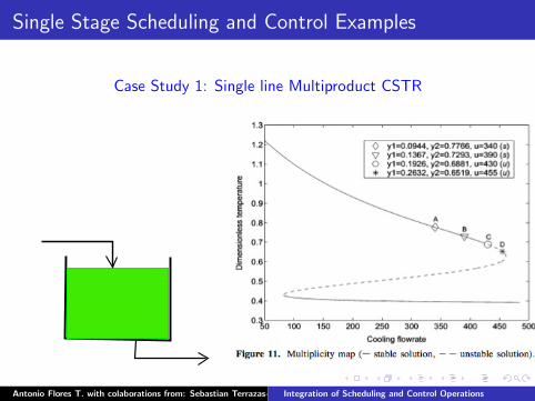
Single Stage Scheduling and Control Examples
Case Study 1: Single line Multiproduct CSTR
Antonio Flores T. with colaborations from: Sebastian Terrazas-Moreno, Miguel Angel Gutierrez-Limon, Ignacio E. Grossmann Universidad Iberoamericana, MexicoIntegration of Scheduling and Control Operations

Single Stage Scheduling and Control Examples
Case Study 1: Single line Multiproduct CSTR
CPU time: 254 s, SbbAntonio Flores T. with colaborations from: Sebastian Terrazas-Moreno, Miguel Angel Gutierrez-Limon, Ignacio E. Grossmann Universidad Iberoamericana, MexicoIntegration of Scheduling and Control Operations
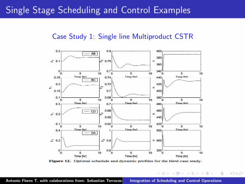
Single Stage Scheduling and Control Examples
Case Study 1: Single line Multiproduct CSTR
Antonio Flores T. with colaborations from: Sebastian Terrazas-Moreno, Miguel Angel Gutierrez-Limon, Ignacio E. Grossmann Universidad Iberoamericana, MexicoIntegration of Scheduling and Control Operations
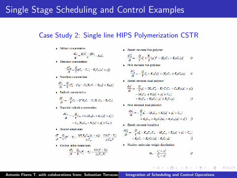
Single Stage Scheduling and Control Examples
Case Study 2: Single line HIPS Polymerization CSTR
Antonio Flores T. with colaborations from: Sebastian Terrazas-Moreno, Miguel Angel Gutierrez-Limon, Ignacio E. Grossmann Universidad Iberoamericana, MexicoIntegration of Scheduling and Control Operations
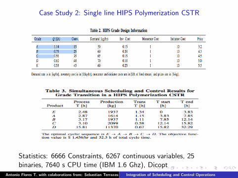
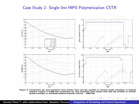
Case Study 2: Single line HIPS Polymerization CSTR
Statistics: 6666 Constraints, 6267 continuous variables, 25binaries, 7640 s CPU time (IBM 1.6 Ghz), Dicopt
Antonio Flores T. with colaborations from: Sebastian Terrazas-Moreno, Miguel Angel Gutierrez-Limon, Ignacio E. Grossmann Universidad Iberoamericana, MexicoIntegration of Scheduling and Control Operations
Case Study 2: Single line HIPS Polymerization CSTR
Antonio Flores T. with colaborations from: Sebastian Terrazas-Moreno, Miguel Angel Gutierrez-Limon, Ignacio E. Grossmann Universidad Iberoamericana, MexicoIntegration of Scheduling and Control Operations
Single Stage Scheduling and Control Examples
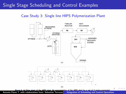
Case Study 3: Single line HIPS Polymerization Plant
Antonio Flores T. with colaborations from: Sebastian Terrazas-Moreno, Miguel Angel Gutierrez-Limon, Ignacio E. Grossmann Universidad Iberoamericana, MexicoIntegration of Scheduling and Control Operations
Single Stage Scheduling and Control Examples
Case Study 3: Single line HIPS Polymerization Plant
Antonio Flores T. with colaborations from: Sebastian Terrazas-Moreno, Miguel Angel Gutierrez-Limon, Ignacio E. Grossmann Universidad Iberoamericana, MexicoIntegration of Scheduling and Control Operations
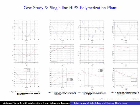
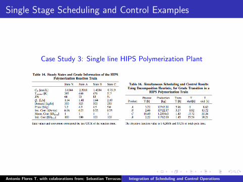
Case Study 3: Single line HIPS Polymerization Plant
Antonio Flores T. with colaborations from: Sebastian Terrazas-Moreno, Miguel Angel Gutierrez-Limon, Ignacio E. Grossmann Universidad Iberoamericana, MexicoIntegration of Scheduling and Control Operations
Single Stage Scheduling and Control Examples
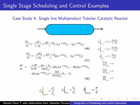
Case Study 4: Single line Multiproduct Tubular Catalytic Reactor
Antonio Flores T. with colaborations from: Sebastian Terrazas-Moreno, Miguel Angel Gutierrez-Limon, Ignacio E. Grossmann Universidad Iberoamericana, MexicoIntegration of Scheduling and Control Operations
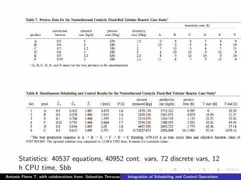
Statistics: 40537 equations, 40952 cont. vars, 72 discrete vars, 12h CPU time, Sbb
Antonio Flores T. with colaborations from: Sebastian Terrazas-Moreno, Miguel Angel Gutierrez-Limon, Ignacio E. Grossmann Universidad Iberoamericana, MexicoIntegration of Scheduling and Control Operations

Case Study 4: Single line Tubular Catalytic Reactor
Antonio Flores T. with colaborations from: Sebastian Terrazas-Moreno, Miguel Angel Gutierrez-Limon, Ignacio E. Grossmann Universidad Iberoamericana, MexicoIntegration of Scheduling and Control Operations
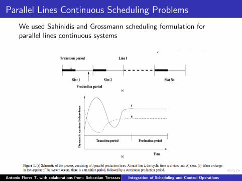
Parallel Lines Continuous Scheduling Problems
We used Sahinidis and Grossmann scheduling formulation forparallel lines continuous systems
Antonio Flores T. with colaborations from: Sebastian Terrazas-Moreno, Miguel Angel Gutierrez-Limon, Ignacio E. Grossmann Universidad Iberoamericana, MexicoIntegration of Scheduling and Control Operations
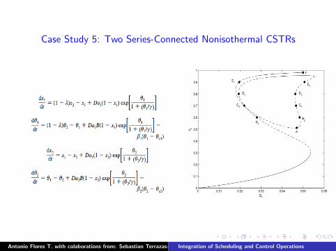
Case Study 5: Two Series-Connected Nonisothermal CSTRs
Antonio Flores T. with colaborations from: Sebastian Terrazas-Moreno, Miguel Angel Gutierrez-Limon, Ignacio E. Grossmann Universidad Iberoamericana, MexicoIntegration of Scheduling and Control Operations
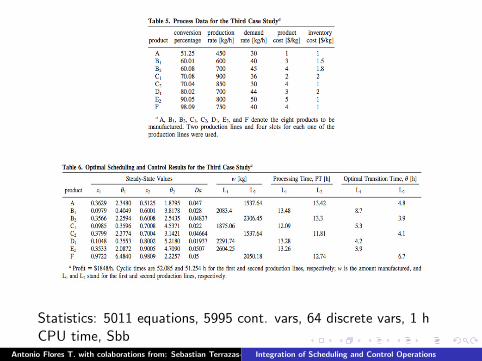
Statistics: 5011 equations, 5995 cont. vars, 64 discrete vars, 1 hCPU time, Sbb
Antonio Flores T. with colaborations from: Sebastian Terrazas-Moreno, Miguel Angel Gutierrez-Limon, Ignacio E. Grossmann Universidad Iberoamericana, MexicoIntegration of Scheduling and Control Operations

Case Study 5: Two Series-Connected Nonisothermal CSTRs
Antonio Flores T. with colaborations from: Sebastian Terrazas-Moreno, Miguel Angel Gutierrez-Limon, Ignacio E. Grossmann Universidad Iberoamericana, MexicoIntegration of Scheduling and Control Operations
A Multiobjective Optimization Approach for SC problems
I Many Engineering problems feature conflicting objectives
I Until now dynamic transitions have been converted intoeconomic profits by using weighting functions so a singleobjective function was used
I However improved optimal solutions can be obtained bysolving SC problems as Multiobjective optimization problemsand the subjective choice of weighting functions is avoided
I Instead of computing a single optimal solution the Paretofront is computed
I The designer chooses his/her preferred optimal solution
I Other measurements such as minimum distance from Utopiaregion to a point on the Pareto front can be used
Antonio Flores T. with colaborations from: Sebastian Terrazas-Moreno, Miguel Angel Gutierrez-Limon, Ignacio E. Grossmann Universidad Iberoamericana, MexicoIntegration of Scheduling and Control Operations
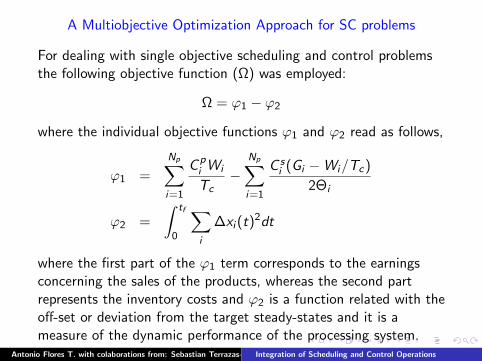
A Multiobjective Optimization Approach for SC problems
For dealing with single objective scheduling and control problemsthe following objective function (Ω) was employed:
Ω = ϕ1 − ϕ2
where the individual objective functions ϕ1 and ϕ2 read as follows,
ϕ1 =
Np∑i=1
Cpi Wi
Tc−
Np∑i=1
C si (Gi −Wi/Tc )
2Θi
ϕ2 =
∫ tf
0
∑i
∆xi (t)2dt
where the first part of the ϕ1 term corresponds to the earningsconcerning the sales of the products, whereas the second partrepresents the inventory costs and ϕ2 is a function related with theoff-set or deviation from the target steady-states and it is ameasure of the dynamic performance of the processing system.
Antonio Flores T. with colaborations from: Sebastian Terrazas-Moreno, Miguel Angel Gutierrez-Limon, Ignacio E. Grossmann Universidad Iberoamericana, MexicoIntegration of Scheduling and Control Operations
A Multiobjective Optimization Approach for SC problems
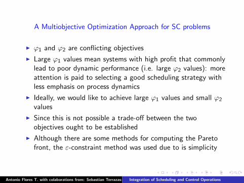
I ϕ1 and ϕ2 are conflicting objectives
I Large ϕ1 values mean systems with high profit that commonlylead to poor dynamic performance (i.e. large ϕ2 values): moreattention is paid to selecting a good scheduling strategy withless emphasis on process dynamics
I Ideally, we would like to achieve large ϕ1 values and small ϕ2
values
I Since this is not possible a trade-off between the twoobjectives ought to be established
I Although there are some methods for computing the Paretofront, the ε-constraint method was used due to is simplicity
Antonio Flores T. with colaborations from: Sebastian Terrazas-Moreno, Miguel Angel Gutierrez-Limon, Ignacio E. Grossmann Universidad Iberoamericana, MexicoIntegration of Scheduling and Control Operations
A Multiobjective Optimization Approach for SC problems
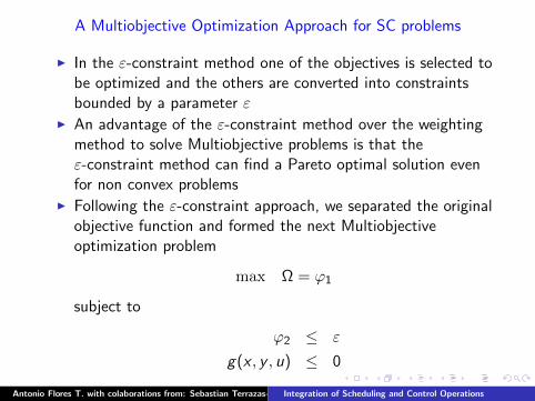
I In the ε-constraint method one of the objectives is selected tobe optimized and the others are converted into constraintsbounded by a parameter ε
I An advantage of the ε-constraint method over the weightingmethod to solve Multiobjective problems is that theε-constraint method can find a Pareto optimal solution evenfor non convex problems
I Following the ε-constraint approach, we separated the originalobjective function and formed the next Multiobjectiveoptimization problem
max Ω = ϕ1
subject to
ϕ2 ≤ ε
g(x , y , u) ≤ 0
Antonio Flores T. with colaborations from: Sebastian Terrazas-Moreno, Miguel Angel Gutierrez-Limon, Ignacio E. Grossmann Universidad Iberoamericana, MexicoIntegration of Scheduling and Control Operations
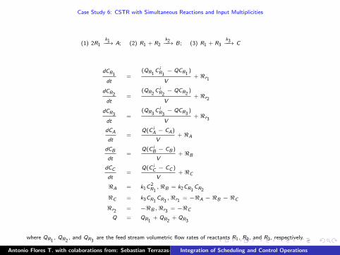
Case Study 6: CSTR with Simultaneous Reactions and Input Multiplicities
(1) 2R1k1−−→ A; (2) R1 + R2
k2−−→ B; (3) R1 + R3k3−−→ C
dCR1
dt=
(QR1C i
R1− QCR1
)
V+ <r1
dCR2
dt=
(QR2C i
R2− QCR2
)
V+ <r2
dCR3
dt=
(QR3C i
R3− QCR3
)
V+ <r3
dCA
dt=
Q(C iA − CA)
V+ <A
dCB
dt=
Q(C iB − CB )
V+ <B
dCC
dt=
Q(C iC − CC )
V+ <C
<A = k1C 2R1,<B = k2CR1
CR2
<C = k3CR1CR3
,<r1= −<A − <B − <C
<r2= −<B ,<r3
= −<C
Q = QR1+ QR2
+ QR3
where QR1, QR2
, and QR3are the feed stream volumetric flow rates of reactants R1, R2, and R3, respectively.
Antonio Flores T. with colaborations from: Sebastian Terrazas-Moreno, Miguel Angel Gutierrez-Limon, Ignacio E. Grossmann Universidad Iberoamericana, MexicoIntegration of Scheduling and Control Operations

Table: Operating Conditions Leading to the Manufacture of the A, B,and C Products of the Second Case Study
Product Demand rate (Kg/h) Product cost ($/Kg) Inventory cost ($/Kg)A 5 500 1.0B 10 400 1.5C 15 600 1.8
0 5 10 15 20 25 30
1.6
1.8
2
2.2
2.4
2.6
2.8
3
3.2
3.4
3.6
x 104
φ2 x 10
−5
φ1
2
1
Figure: Pareto curve for the second case of study. The coordinates forthe first and second points are: [φ1
2, φ11] = [5x10⁻⁵, 25590] and [φ2
2, φ21]
= [2.5x10⁻⁴, 35250], respectively.Antonio Flores T. with colaborations from: Sebastian Terrazas-Moreno, Miguel Angel Gutierrez-Limon, Ignacio E. Grossmann Universidad Iberoamericana, MexicoIntegration of Scheduling and Control Operations

Table: Results for the the first optimal operating point. The objectivefunction values are: φ1
2 = 5x10⁻⁵ and φ11 = 25590.Total cycle time is
659.3 h.
Process Prod rate w Transition T start T endSlot Prod time (min) (Kg/min) (Kg) time (min) (min) (min)
1 A 49.423 66.700 3296.519 10 0.000 59.4232 B 92.456 71.310 6593.038 10 59.423 161.8793 C 447.425 89.520 40053.458 50 161.879 659.304
Table: Results for the the second optimal operating point. The objectivefunction values are: φ2
2 = 2.5x10⁻⁴ and φ21 = 35250.Total cycle time is
327.8 h.
Process Prod rate w Transition T start T endSlot Prod time (min) (Kg/min) (Kg) time (min) (min) (min)
1 B 45.969 71.310 3278.079 10 0.000 55.9692 A 24.573 66.700 1639.039 10 55.969 90.5433 C 227.265 89.520 20344.778 10 90.543 327.808
Antonio Flores T. with colaborations from: Sebastian Terrazas-Moreno, Miguel Angel Gutierrez-Limon, Ignacio E. Grossmann Universidad Iberoamericana, MexicoIntegration of Scheduling and Control Operations
0 2 4 6 8 100
0.25
0.5
0.75
C, m
ol/lt
0 2 4 6 8 100
0.2
0.4
0.6
0.8
1
u
0 2 4 6 8 100
0.1
0.2
0.3
0.4
C,
mol/lt
0 2 4 6 8 100
0.2
0.4
0.6
0.8
1
u
0 10 20 30 40 500
0.2
0.4
0.6
0.8
time, m
C,
mo
l/lt
0 10 20 30 40 50−0.1
0
0.1
0.2
0.3
0.4
time, m
u
CA
CB
CC
u2
u3
AB
BC
CA
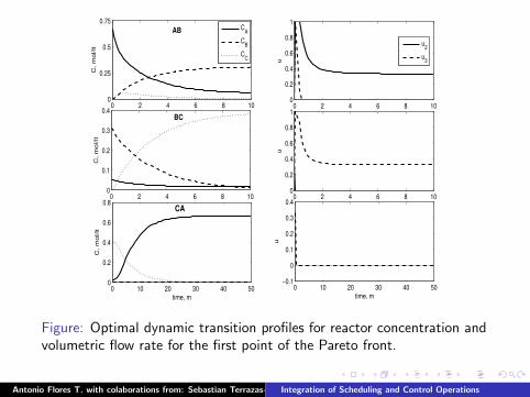
Figure: Optimal dynamic transition profiles for reactor concentration andvolumetric flow rate for the first point of the Pareto front.
Antonio Flores T. with colaborations from: Sebastian Terrazas-Moreno, Miguel Angel Gutierrez-Limon, Ignacio E. Grossmann Universidad Iberoamericana, MexicoIntegration of Scheduling and Control Operations

0 2 4 6 8 100
0.1
0.2
0.3
0.4
0.5
C, m
ol/lt
0 2 4 6 8 100
0.2
0.4
0.6
0.8
1
u
0 2 4 6 8 100
0.2
0.4
0.6
0.8
C,
mo
l/lt
0 2 4 6 8 100
0.2
0.4
0.6
0.8
1
u
0 2 4 6 8 100
0.1
0.2
0.3
0.4
time, m
C,
mo
l/lt
0 2 4 6 8 100
0.1
0.2
0.3
0.4
time, m
u
CA
CB
CC
u2
u3
BA
AC
CB
Figure: Optimal dynamic transition profiles for reactor concentration andvolumetric flow rate for the second point of the Pareto front.
Antonio Flores T. with colaborations from: Sebastian Terrazas-Moreno, Miguel Angel Gutierrez-Limon, Ignacio E. Grossmann Universidad Iberoamericana, MexicoIntegration of Scheduling and Control Operations
Conclusions
I An algorithmic framework for addressing Scheduling andControl problems using a MIDO formulation was presented
I The SC MIDO formulation was successfully applied to severalcase studies of varying complexity such as chemical reactorsfeaturing strong nonlinear behavior, bifurcation points,unstable operating regions, multiple steady-states
I Presently the SC MIDO formulation only computes off-lineoptimal control policies, no consideration of the effect ofuncertainties or disturbances
Antonio Flores T. with colaborations from: Sebastian Terrazas-Moreno, Miguel Angel Gutierrez-Limon, Ignacio E. Grossmann Universidad Iberoamericana, MexicoIntegration of Scheduling and Control Operations

Future Work
I Real-Time Optimization for Scheduling and Control
I Stochastic Scheduling and Control
I Large-Scale Scheduling and Control
I Integration of Planning, Scheduling and Control
Antonio Flores T. with colaborations from: Sebastian Terrazas-Moreno, Miguel Angel Gutierrez-Limon, Ignacio E. Grossmann Universidad Iberoamericana, MexicoIntegration of Scheduling and Control Operations

1. Antonio Flores-Tlacuahuac, I.E. Grossmann, “An Effective MIDO Approach for the Simultaneous CyclicScheduling and Control of Polymer Grade Transition Operations”, In W. Marquardt and C. Pantelides,
editors. In 16th European Symposium on Computer Aided Process Engineering and 9th InternationalSymposium on Process System Engineering, pages 1221-1226, Elsevier, 2006. ISBN: 978-0-444-52970-1.
2. Antonio Flores-Tlacuahuac, Ignacio E. Grossmann, “Simultaneous Cyclic Scheduling and Control of aMultiproduct CSTR Reactor”, Industrial and Engineering Chemistry Research, 45,20,6698-6712(2006)
3. Sebastian Terrazas-Moreno, Antonio Flores-Tlacuahuac, Ignacio E. Grossmann, “Simultaneous CyclicScheduling and Optimal Control of Polymerization Reactors”, AIChE Journal, 53,9,2301-2315(2007)
4. Sebastian Terrazas-Moreno, Antonio Flores-Tlacuahuac, Ignacio E. Grossmann, “A Lagrangean Heuristicfor the Scheduling and Control of Polymerization Reactors”, AIChE Journal, 54,1,163-182(2008)
5. Sebastian Terrazas-Moreno, Antonio Flores-Tlacuahuac, Ignacio E. Grossmann, “Simultaneous Design,Scheduling and Optimal Control of a Methyl-Methacrylate Continuous Polymerization Reactor”, AmericanInstitute of Chemical Engineers Journal, 54,12,3160-3170(2008)
6. Antonio Flores-Tlacuahuac, Ignacio E. Grossmann, “Simultaneous Scheduling and Control of MultiproductContinuous Parallel Lines”, Industrial and Engineering Chemistry Research, 49,17,7909-7921(2010)
7. Antonio Flores-Tlacuahuac, Ignacio E. Grossmann, “Simultaneous Cyclic Scheduling and Control ofTubular Reactors: Single Production Lines”, Industrial and Engineering Chemistry Research,49,22,11453-11463(2010)
8. Antonio Flores-Tlacuahuac, Ignacio E. Grossmann, “Simultaneous Cyclic Scheduling and Control ofMultiproduct Tubular Reactors in Parallel Lines”, Industrial and Engineering Chemistry Research, 50 (13),8086-8096, 2011
9. Miguel Angel Gutierrez-Limon, Antonio Flores-Tlacuahuac, Ignacio E. Grossmann, “A MultiObjectiveOptimization Approach for the Simultaneous Single Line Scheduling and Control of CSTRs”, Submitted to:Industrial and Engineering Chemsirty Research, 2011.
10. Miguel Angel Gutierrez-Limon, Antonio Flores-Tlacuahuac, Ignacio E. Grossmann, “A Real TimeOptimization Approach for Simultaneous Single Line Scheduling and Control Problems”, Underpreparation, 2011.
Antonio Flores T. with colaborations from: Sebastian Terrazas-Moreno, Miguel Angel Gutierrez-Limon, Ignacio E. Grossmann Universidad Iberoamericana, MexicoIntegration of Scheduling and Control Operations