Embed Size (px)
Citation preview

Procesos distribuidos en la generación y transporte de escorrentía y sedimento en olivar a diferentes escalas
Distributed processes in the runoff and sediment generation and transport in olive groves at different scales.
AutoraMaría Burguet Marimón
Dirigido porDr. Jose Alfonso Gómez || Dra. Encarnación V. Taguas
Departamento de Agronomía. Universidad de Córdoba
2015
Tes
is D
octo
ral
M
aría
Bur
guet
Mar
imón
Soil erosion and land degradation are two of the major environmental problems in Spain, which affect the South and South-East of the peninsula. Therefore, it is essential to fully understand soil degradation processes so that solutions which will decrease -and ideally eliminate- that degradation can be provided. The general objective of this doctoral thesis is to improve and to contribute to alternative strategies to enhance soil and water conservation practices. The initial hypothesis is that it is possible to characterize and model runoff and sediment fluxes associated to small crop watersheds from experimental studies at different scales (one-off measurements scale, runoff plots in hillslopes scale and watershed scale). For this purpose, the doctoral thesis is divided into two parts: the first one corresponds to the experimental work carried out in the field and laboratory and, a second part, addresses the calibration of a physical distributed model which would serve as a tool to synthesize and understand the decisive processes involved in the water and sediment fluxes within a watershed.
In the first experimental part, two methodologies are presented for on the one hand, locate runon-runoff areas in olive crops and, on the other hand, understand the sediment transport and storage processes at the hillslope scale. For the first assumption, soil water repellency measured in four different olive crops with different overall soil management (abandoned, conventional tillage, herbicide and cover crop) has been gathering. The methodology used was the Water Drop Penetration Time test (WDPT). Regarding the study of the sediment transport and storage, three runoff plots were established in a hillslope in which bare soil and vegetation strips were combined alternately. Bare soil was tagged with magnetic iron as a tracer. At the watershed level, hydrological data (precipitation, runoff, peak flow, sediment loads) measured in two olive crop watershed was used to calibrate a physical distributed model. The model chosen was SEDD as it allows, on the one hand, the discretization of a watershed into morphological units, it predicts sediment delivery ratio at both geomorphological unit and watershed scale, it is based on the RUSLE and it also easy to couple within a Geographical Information System.

TITULO: Procesos distribuidos en la generación y transporte de escorrentía ysedimento en olivar a diferentes escalas.
AUTOR: Maria Burguet Marimon
© Edita: Servicio de Publicaciones de la Universidad de Córdoba. 2015 Campus de RabanalesCtra. Nacional IV, Km. 396 A14071 Córdoba
www.uco.es/[email protected]
UNIVERSIDAD DE CÓRDOBA
DEPARTAMENTO DE AGRONOMÍA
PROGRAMA DE DOCTORADO
DINÁMICA DE LOS FLUJOS BIOGEOQUÍMICOS Y SUS APLICACIONES
TESIS DOCTORAL
Procesos distribuidos en la generación y transporte de
escorrentía y sedimento en olivar a diferentes escalas.
Distributed processes in the runoff and sediment generation and transport in olive
groves at different scales.
Autora
María Burguet Marimón
Directores
Dr. José Alfonso Gómez Calero
Dra. Encarnación V. Taguas Ruíz
Tesis financiada por el programa de formación de personal investigador “Junta para la Ampliación de Estudios” (subprograma JAE-predoc) del Consejo Superior de Investigaciones Científicas (CSIC).
Instituto de Agricultura Sostenible-CSIC
UNIVERSIDAD DE CÓRDOBA
DEPARTAMENTO DE AGRONOMÍA
TESIS DOCTORAL
Procesos distribuidos en la generación y transporte de
escorrentía y sedimento en olivar a diferentes escalas.
presentada por MARÍA BURGUET MARIMÓN en satisfacción de los requisitos necesarios para la obtención del grado de DOCTOR EN GEOGRAFÍA.
Los Directores,
Dr. José Alfonso Gómez Calero
Científico titular Dpto. Agronomía Instituto de Agricultura Sostenible (CSIC)
Córdoba, 2015
Dra. Encarnación V. Taguas Ruíz
Profesora Contratada Doctora Dpto. Ingeniería Rural-Proyectos Universidad de Córdoba
TÍTULO DE LA TESIS: Procesos distribuidos en la generación y transporte de escorrentía y sedimento en olivar a diferentes escalas.
DOCTORANDO/A: María Burguet Marimón
INFORME RAZONADO DEL/DE LOS DIRECTOR/ES DE LA TESIS
(se hará mención a la evolución y desarrollo de la tesis, así como a trabajos y publicaciones derivados de la misma).
Encarnación V. Taguas Ruíz, Profesora Contratada de la Universidad de Córdoba y
José Alfonso Gómez Calero, Científico Titular del IAS-CSIC, como directores de la
tesis doctoral de la alumna del Programa de Doctorado ‘Dinámica de Flujos
Biogeoquímicos y su Aplicación’, María Burguet
INFORMAN,
Que durante su periodo como becaria de la Junta de Ampliación de Estudios (JAE)
participó activamente en diferentes actividades formativas de carácter internacional: en
el BSG Post-Graduate Research Training Workshop (Windsor, UK, 12-15 Diciembre
2011) organizado por la British Society for Geomorphology; así mismo realizó una
estancia de 90 días en el Departamento de Geografía de la University of Exeter (Reino
Unido) desde Septiembre de 2012 a Diciembre de 2012 con el Dr. Richard Brazier. El
objetivo de esta estancia fue estudiar los flujos de carbono en una cuenca olivarera
mediante el uso del isótopo estable δ13C como trazador con el fin de entender las
dinámicas de erosión y degradación del suelo en áreas semi-áridas cultivadas. En
Enero de 2013 fue premiada con una 'Young Scientist's Travel Award' para participar
en el European Geoscience Union (EGU) con el trabajo 'The use of magnetic iron
oxide as a tracer to determine vegetation trapping efficiency in Southern Spain at
hillslope scale' correspondiente al tercer capítulo de esta tesis doctoral. Asimismo,
parte de los resultados de cada uno de los capítulos han sido presentados en
diferentes sesiones en el congreso European Geoscience Union (EGU). Estas
estancias han complementado su formación predoctoral que se ha articulado con una
combinación de trabajos experimentales centrados en el impacto que los procesos de
hidrofobicidad pudieran tener en olivares de diferente grado de intensificación
(Capítulo 2 de su tesis doctoral), efecto de retención de bandas e cubiertas vegetales
en ladera mediante ensayos con lluvia simulada y natural incorporando trazadores de
erosión (Capítulo 3 de su tesis doctoral), y modelización del aporte de sedimento en
diferentes áreas de pequeñas cuencas de olivar mediante la calibración del modelo
SEDD en dos olivares condiciones edafoclimáticas diferentes (Capítulo 4 de su tesis
doctoral). Durante todo el desarrollo de tu formación predoctoral, la candidata ha
mostrado un elevado grado de dedicación, capacidad y habilidad para el trabajo en
equipo. Todo ello, además de posibilitar la realización de los trabajos de investigación
incluidos en su tesis doctoral, le han permitido alcanzar el grado de madurez y
especialización necesarios para optar al grado de doctor.
Por todo ello, se autoriza la presentación de la tesis doctoral.
Córdoba, 5 de Mayo de 2015
Firma del/de los director/es
Encarnación V. Taguas Ruíz José Alfonso Gómez Calero
I am the rain
Held in disdain
Lotions and potions just add to my fame
The rime that in Spain
Fall on the plain
The truth is I'm ruthless
I can't be contained.
I'm the rain
My friend the wind
To breath he is twinned
Blow high or low high
Tornadoes to spin
My mother the cloud
In widow's black shroud
Gives birth to the earth
Before fields can be ploughed
Up in the sky, we've demand to supply
I am necessity, base of the recipe
I'm the rain
My cousin the snow
Lays blankets below
States that her flakes are
The threads to the soul
My rival the sun
Who ripens the plum
Is feared and revered
He gives sight to the gun
Up in the sky, we've demand to supply
I am necessity, base of the recipe
Up in the sky, we've demand to supply
I am necessity, base of the recipe
I am the rain, am the rain
I am the rain, who's held in disdain
The truth is I'm ruthless, I can't be contained.
Peter Doherty. I am the rain. Grace/Wastelands, 2009

Sencillo e intrincado,
con su tesoro a cuestas
el olivar cavila.
En él no son precisos
ni rosas ni claveles:
sólo estar, siglo a siglo,
serenamente en pie.
Cuanto miramos desde arriba es nuestro,
porque nos mira y somos suyos.
Cae el cielo, y tú me amas,
y el olivar nos ama a ti y a mí.
La tormenta muy pronto
restallará sus látigos. ¿Qué importa?:
ya no sueño dormido ni despierto,
ya te tengo entre olivos.
Mi patria sois; me extinguiré en vosotros
para que empiece todo una vez más.
Antonio Gala, Olivares de Mancha Real


A mis padres

He acabado de recorrer este camino, a veces largo y duro, otras veces corto y lleno de
alegrías...y al final pesan más los buenos momentos que los malos. Son muchas las personas que
me han acompañado en esta travesía, que han aguantado mis miedos y locuras, mis dudas, mis
quebraderos de cabeza, que han sido cómplices de tantos momentos buenos, que han estado ahí
cuando las he necesitado. Pero de todas esas personas, hay una a la que le dedico especialmente
esta tesis. Ella sabe del esfuerzo y dedicación que tiene este trabajo, de las noches sin dormir, de
las tardes volviendo a casa derrotada y con ganas de hablar con ella para que me diese las
palabras de aliento que necesitaba, que 'després de l'ú ve el dos'; una mujer con tantas ganas de
luchar y vivir que era imposible no terminar esta tesis. Una guerrera en todos y cada uno de los
aspectos de su vida; mi amiga y consejera. Es por ella por la que he podido terminar con más
fuerza y ánimo... 'se puede perder una batalla, pero no significa que la guerra se haya perdido'.
Porque a pesar de no estar físicamente presente, te llevo siempre conmigo MAMÁ.
A mi guerrero shaolin, porque una vez siendo pequeña te pregunté ‘¿de dónde vienen
las montañas?’ y me respondiste ‘eso lo puedes saber si estudias Geografía’. Una pregunta y
una respuesta que marcaron lo que soy. Eres mi norte cuando estoy en el sur, papá.
A José Alfonso, mi maestro Po. Porque sin ti no podría haber llegado a la categoría de 'Pequeño
Saltamontes'. Porque siempre has estado ahí, en los momentos críticos y en los relajados. Por
tus explicaciones a pie de campo, por tu implicación en cada experimento, y por tu risa
contagiosa.
A Tani, mi maestra hidróloga indie. Porque la modelización hidrológica no es sólo un número,
es conocer cada detalle de cada evento como si fuera un hijo tuyo. Porque gracias a ti conocí en
una clase de máster a 'elderbar' y a la vez la planificación hidrológica de cuencas. Por animarme
cuando decaía.
A Artemi Cerdà, por haberme invitado en primero de carrera a 'hacer trabajo de campo' e
inocularme el virus de la ciencia.
A Elías Fereres, el jefe de la expedición. Por sus sabios consejos geopolítico-científicos y apoyo
durante mi paso por el IAS.
A Paco Orgaz y a Luca Testi, por ayudarme de la forma en la que lo hicieron, por su cariño y
atención siempre.
A Hava Rapoport, por sus conversaciones en el café/té y por sus pasteles.
A Manolo, a Clemente, a Azahara y a Gema, por su ayuda en el campo de la que tanto he
aprendido (entre otras cosas a diferenciar entre maíz para harina y maíz para palomitas).
A los niños y niñas del laboratorio 1: a Manuela por su paciencia, a Kiki por su cariño, a
Carmen por su energía, a Marga por sus abrazos, a Mónica por su fuerza, a Manuel niño Lama
por ayudarme a saborear la vida, al Doc Elorza por su risa, a Facundo por ser mi compi de
cordada, a Luis por ser mi rival al ‘pachamama’, a Manolo por sus lecturas y luminosidades, a
Macmolder por sus riñas (siempre bien fundamentadas) y saber cogerme cual saco de patatas.
A los Pingos Criminosos, Álvaro y Omar, por enseñarme que hasta en los momentos más
oscuros hay luz (y potensssiales, ecuasssiones de Richardsss y sapflows).

A los IAS-buddies, por las conversaciones a la hora de la comida y los buenos ratos juntos:
Thaïs, Antonio, Carlitros, Carlos, Carmen, David (Gramaje y Ruano), Enri, Héctor, Inma, Liz,
Lola, Mercedes, Paco, Mariluz.
A los chicos del MHA-UCO, en especial a Rafa ‘Glasses’ y a Pedro, por saber estar sin estar en
todo momento.
A la 'familien Vienna': Alicia, Merche, Raúl, Ágata y Paulo, por haberme demostrado que se
pueden tener buenos amigos en la ciencia. Gracias por contagiarme vuestra alegría y ganas de
luchar constantemente.
A Elena, Yeah y Cristina, por vuestra amistad, amor, cariño…y dramas.
A Antonia y a Augusto, por dejarme entrar y formar parte de su familia.
A Steve, porque 'there is nothing to be ashamed about and everything to be proud of'.
A Rocío, mi piedra angular en mi paso por Córdoba, mi nota discordante. Qué habría sido de mí
sin ti, de nuestras vivencias juntas, de estos años de sincera amistad.
A Miguel, el espejo en el que me reflejo. Porque de ti he aprendido el significado de las palabras
'tenacidad' y 'determinación'. Porque siempre estás ahí, en lo bueno y en lo malo.
A mi hermana, mi luz, mi guía, mi mitad. Gracias por luchar siempre a mi lado, gracias por
hacerme ver la vida de una manera más positiva. Gracias por ser tú.
A mis padres, Toni y Nieves, por vuestro apoyo y amor incondicional en todos y cada uno de
los momentos de mi vida. Porque me disteis alas para volar y colchón cuando caí. Gracias por
aguantar mis malos ratos, mis sofocos, mis agobios, mis alegrías y mis penas. Gracias. Gracias.
Gracias.
Olivar, por cien caminos, tus olivitas irán caminando a cien molinos
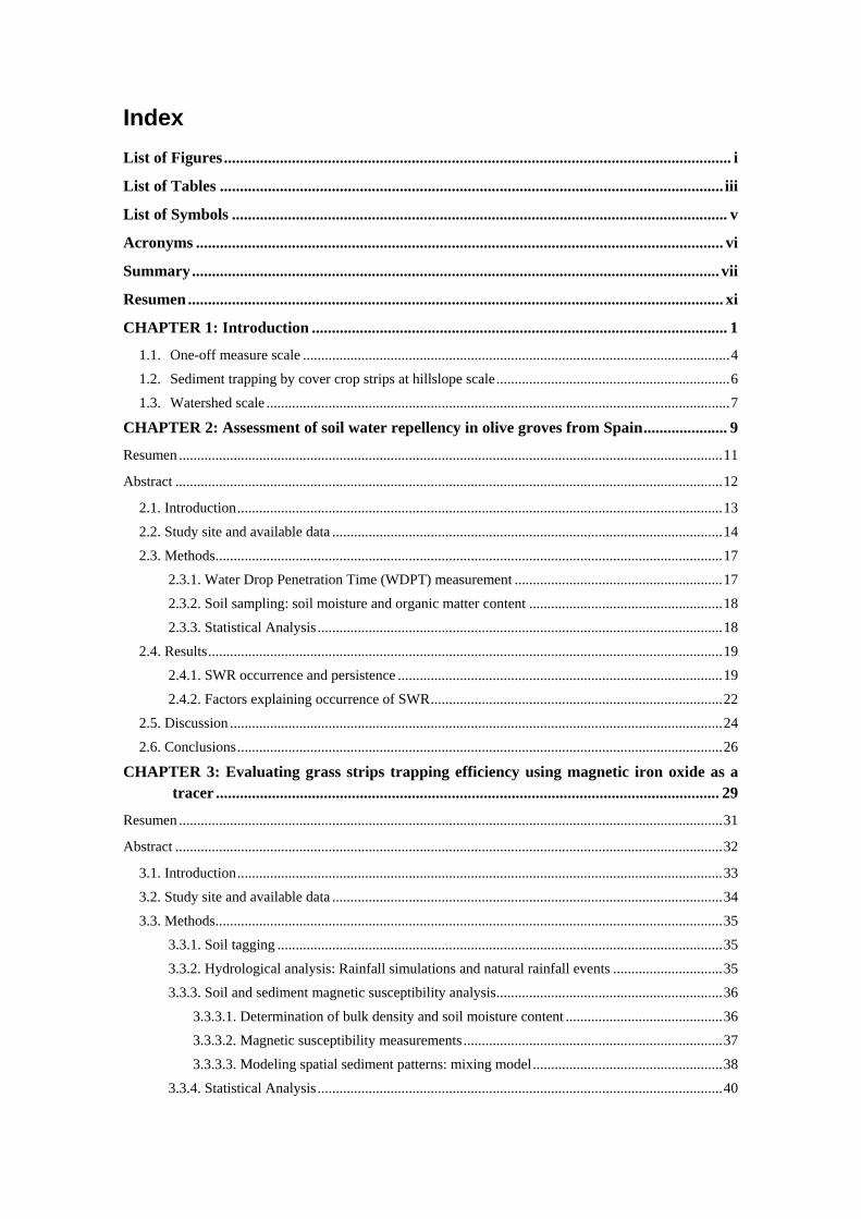
Index
List of Figures ............................................................................................................................... i
List of Tables .............................................................................................................................. iii
List of Symbols ............................................................................................................................ v
Acronyms .................................................................................................................................... vi
Summary .................................................................................................................................... vii
Resumen ...................................................................................................................................... xi
CHAPTER 1: Introduction ........................................................................................................ 1
1.1. One-off measure scale ..................................................................................................................... 4
1.2. Sediment trapping by cover crop strips at hillslope scale ................................................................ 6
1.3. Watershed scale ............................................................................................................................... 7
CHAPTER 2: Assessment of soil water repellency in olive groves from Spain ..................... 9
Resumen ..................................................................................................................................................... 11
Abstract ...................................................................................................................................................... 12
2.1. Introduction ..................................................................................................................................... 13
2.2. Study site and available data ........................................................................................................... 14
2.3. Methods ........................................................................................................................................... 17
2.3.1. Water Drop Penetration Time (WDPT) measurement ......................................................... 17
2.3.2. Soil sampling: soil moisture and organic matter content ..................................................... 18
2.3.3. Statistical Analysis ............................................................................................................... 18
2.4. Results ............................................................................................................................................. 19
2.4.1. SWR occurrence and persistence ......................................................................................... 19
2.4.2. Factors explaining occurrence of SWR ................................................................................ 22
2.5. Discussion ....................................................................................................................................... 24
2.6. Conclusions ..................................................................................................................................... 26
CHAPTER 3: Evaluating grass strips trapping efficiency using magnetic iron oxide as a
tracer .............................................................................................................................. 29
Resumen ..................................................................................................................................................... 31
Abstract ...................................................................................................................................................... 32
3.1. Introduction ..................................................................................................................................... 33
3.2. Study site and available data ........................................................................................................... 34
3.3. Methods ........................................................................................................................................... 35
3.3.1. Soil tagging .......................................................................................................................... 35
3.3.2. Hydrological analysis: Rainfall simulations and natural rainfall events .............................. 35
3.3.3. Soil and sediment magnetic susceptibility analysis .............................................................. 36
3.3.3.1. Determination of bulk density and soil moisture content ........................................... 36
3.3.3.2. Magnetic susceptibility measurements ....................................................................... 37
3.3.3.3. Modeling spatial sediment patterns: mixing model .................................................... 38
3.3.4. Statistical Analysis ............................................................................................................... 40

3.4. Results ............................................................................................................................................. 40
3.4.1. Rainfall, runoff and sediment measurements ....................................................................... 40
3.4.2. Soil redistribution and source of sediments ......................................................................... 44
3.5. Discussion ....................................................................................................................................... 47
3.6. Conclusions ..................................................................................................................................... 49
CHAPTER 4: Exploring calibration strategies of SEDD model in two olive orchard
watersheds ..................................................................................................................... 51
Resumen ..................................................................................................................................................... 53
Abstract ...................................................................................................................................................... 54
4.1. Introduction ..................................................................................................................................... 55
4.2. Study site and available data ........................................................................................................... 56
4.2.1. Catchment location and description ..................................................................................... 56
4.2.2. Hydrological data ................................................................................................................. 57
4.3. Methods ........................................................................................................................................... 58
4.3.1. SEDD model (Sediment Delivery Distributed model) ......................................................... 58
4.3.1.1. Model components ..................................................................................................... 58
4.3.1.2. Geomorphological unit determination ........................................................................ 59
4.3.1.3. Sediment yield calculations ........................................................................................ 59
4.3.1.4. Sensitivity analysis and model calibration ................................................................. 61
4.4. Results ............................................................................................................................................. 62
4.4.1. Geomorphological and hydrological characteristics of the watersheds ............................... 62
4.4.2. Analysis of calibration strategies: effects of R-value and C-value on β features. ................ 64
4.4.3. Model calibration ................................................................................................................. 67
4.4.4. Characterization of the spatio-temporal variability of soil loss, sediment yield and SDR ... 70
4.4.4.1. Hydrological year and watershed scale ...................................................................... 70
4.4.4.2. Geomorphological unit scale ...................................................................................... 72
4.5. Discussion ....................................................................................................................................... 75
4.6. Conclusions ..................................................................................................................................... 77
CHAPTER 5: General Conclusions ......................................................................................... 79
5.1. General Conclusions ....................................................................................................................... 81
5.2. Future Research Lines ..................................................................................................................... 82
APPENDIX 1: Hydrological attributes of the observed events for the study period in
Setenil watershed .......................................................................................................... 83
APPENDIX 2: Hydrological attributes of the observed events for the study period in
Conchuela watershed .................................................................................................... 89
APPENDIX 3: SEDD model calibration for Setenil and Conchuela watersheds ................ 95
REFERENCES .......................................................................................................................... 99
i
List of Figures
Figure 2.1. Sampling points location. Cordoba sites include the cover crop (CC), conventional tillage
(CT) and herbicide (H) orchards; Valencia site includes the abandoned (AB) orchard ............................. 15
Figure 2.2. Study sites: A) Cover crop (CC), B) Conventional tillage (CT), C) Herbicide (H) and D)
Abandoned (AB). ....................................................................................................................................... 17
Figure 2.3. Scheme of the sampling transects performed in every olive tree every 10 cm (red lines) and
droplet for the assessment of soil water repellency (WDPT). .................................................................... 18
Figure 2.4. Spatial distribution of WDPT in relation to the tree trunk (normalized dividing by the canopy
radius in each transect) in the cover crop (CC) olive orchard during the three seasons measured. ............ 21
Figure 2.5. Second grade polynomial relationship between the average OM (%) content and median
WDPT (s) values for the four studied orchards during autumn and summer surveys. ............................... 24
Figure 3.1. Plot location in Spain and aerial view of the plots in the hillslope. ......................................... 34
Figure 3.2. Plot magnetic susceptibility, tagging map and sampling scheme (in meters). Grey colour
represents the position of the vegetation stripes, not tagged, while the white area marks the bare soil
tagged with magnetic iron oxide. Circles show the position of the raingauges during the rainfall
simulation. Dotted diamonds depict the position of the sprinkler nozzles. ................................................ 35
Figure 3.3. Soil sampling for magnetic susceptibility determination (left) and mass magnetic
susceptibility in the laboratory (right). ....................................................................................................... 37
Figure 3.4. MS2D field loop and MS2B laboratory sensor calibration for mapping magnetic
susceptibility along the plots. ..................................................................................................................... 38
Figure 3.5. Relationship between the normalized magnetic susceptibility of the ten aggregate size
(cs=χi/χ) and the mass normalized clay content (ci/c). ............................................................................... 39
Figure 3.6. Relationship between the average normalized magnetic susceptibility of the normalized depth
intervals (hi/h) and the mass normalized clay content (cd=χi/χ). ............................................................... 40
Figure 3.7. Sediment magnetic susceptibility variation during the rainfall simulations in plot B ............ .45
Figure 3.8. Average values and tipic error bars of the sediment contribution from the tagged (area
originally bare between cover crop strips) and untagged (area originally covered by vegetation strips)
areas to the total sediment. ........................................................................................................................ 46
Figure 3.9. Soil movement along plot B. Dotted lines show the extension of each vegetation strip.
Negative values denote areas with net soil displacement and positive values areas with net soil deposition.47
Figure 4.1 Location and view of the study catchments: (up) situation in Spain; (below) aerial
ortophotography with their limits and their geomorphological units ......................................................... 57
Figure 4.2. â distribution for biweekly C-values and equal to 0.30 for the best fitted scenario in each
watershed (Setenil Rt=Rp; Conchuela Rt=Rq) .......................................................................................... .66
Figure 4.3. Scatterplots of observed-predicted values derived from the model calibration in the study
catchments ................................................................................................................................................. .67
Figure 4.4. Event SDRs histogram for each geomorphological unit in Setenil watershed ....................... .72
Figure 4.5. Event SDRs histogram for each geomorphological unit in Conchuela watershed. ................. 74

ii
Figure A.1. Model predictions for C-RUSLE values equal to 0.30 for the best fitted scenario in each
watershed. The dotted box is zoomed in on the right plots ....................................................................... .97
Figure A.2. Model predictions for C-RUSLE values equal to 0.30 for the best fitted scenario in each
watershed. The dotted box is zoomed in on the right plots. ...................................................................... 98
iii
List of Tables
Table 2.1. Site characteristics. ................................................................................................................... 16
Table 2.2. WDPT values (Max.= maximum; Min.= minimum, Avg.= average; Std.= standard deviation,
CV= coefficient of variation; n=184) and Tukey HSD test for the autumn survey. Different letters mean
significant differences at p ≤0.05. .............................................................................................................. 19
Table 2.3. WDPT values (Max.= maximum; Min.= minimum, Avg.= average; Std.= standard deviation,
CV= coefficient of variation; n=184) and Tukey HSD test for the winter survey. Different letters mean
significant differences at p ≤0.05. .............................................................................................................. 20
Table 2.4. WDPT values (Max. = maximum; Min.= minimum, Avg.= average; Std.= standard deviation,
CV= coefficient of variation; n=184) and Tukey HSD test for the winter survey. Different letters mean
significant differences at p ≤0.05. .............................................................................................................. 20
Table 2.5. Median values of the samples of Water Drop Penetration Time (WDPT) and average values of
Organic Matter (OM) content and Soil Moisture content (θ %) in relation to the soil management. ......... 23
Table 3.1. Attributes of the six rainfall simulations (CUC= Christiansen Uniformity Coefficient; P= event
rainfall; RI= average rainfall intensity; TRG= Time to runoff generation; Cum. run= Cumulative runoff;
R. rate= Runoff rate; C= Runoff coefficient; Qp= Peak flow; S.C. = Sediment concentration; Max. S.C =
Maximum sediment concentration; i-ii= first and second half of the rainfall simulations; * = low value of
the CUC coefficient as one of the measuring buckets fell). ....................................................................... 42
Table 3.2. Average values of the attributed of the six rainfall simulations (CUC= Christiansen Uniformity
Coefficient; P= event rainfall; RI= average rainfall intensity; TRG= Time to runoff generation; Cum.
run= Cumulative runoff; R. rate= Runoff rate; C=Runoff coefficient; Qp= Peak flow; S.C=Sediment
concentration; Max. S.C= Maximum sediment concentration; i-ii= first and second half of the rainfall
simulations). ............................................................................................................................................... 43
Table 3.3. Weighted values (average) of the collected runoff sediment sample magnetic susceptibility and
particle size for each rainfall simulation ..................................................................................................... 44
Table 4.1. Properties of the geomorphological units in Setenil and Conchuela watershed. ...................... 63
Table 4.2. Hydrological attributes of the observed events for the study period in Setenil watershed (P=
event rainfall; I30= maximum intensity in 30 minutes; Qp= peak flow; Q= runoff; L= sediment discharge;
Rp= rainfall erosivity (Williams factor in MJ mm ha-1 h-1). ........................................................................ 63
Table 4.3. Hydrological attributes of the observed events for the study period in Conchuela watershed
(P= event rainfall; I30= maximum intensity in 30 minutes; Qp= peak flow; Q= runoff; L= sediment
discharge; Rq= runoff erosivity (Williams factor in MJ mm ha-1 h-1). ........................................................ 64
Table 4.4. Summary of the analysis of the combination of the different R-Williams runoff factor for
Setenil watershed using a biweekly C-RUSLE value. ................................................................................ 65
Table 4.5. Summary of the analysis of the combination of the different R-Williams runoff factor for
Conchuela watershed using a biweekly C-RUSLE value. .......................................................................... 65
Table 4.6. Seasonal C-values for Setenil watershed. ................................................................................. 68
Table 4.7. Seasonal C-values for Conchuela watershed. ........................................................................... 69
Table 4.8. Sediment delivery ratios and erosion values for each hydrological year for the Rt=Rp scenario
in Setenil watershed (SDRw: Sediment Delivery ratio of the watershed; P=precipitation). ....................... 71
Table 4.9. Sediment delivery ratios and erosion values for each hydrological year for the Rt=Rq scenario
in Conchuela watershed (SDRw: Sediment Delivery ratio of the watershed; P=precipitation). ................. 71
Table 4.10. Mean and standard deviation of annual contributions of each geomorphological unit in
Setenil and Conchuela watersheds on the total soil losses and potential erosion, sediment delivery ratios
(SDR) and percentage/contribution on the annual total sediment yield. .................................................... 73

iv
Table A.1. Hydrological attributes of the observed events for the study period in Setenil watershed (P=
event rainfall; I30= maximum intensity in 30 minutes; Qp= peak flow; Q= runoff; L= sediment discharge;
Rp= rainfall erosivity (Williams factor). .................................................................................................... 85
Table A.2. Hydrological attributes of the observed events for the study period in Conchuela watershed
(P= event rainfall; I30= maximum intensity in 30 minutes; Qp= peak flow; Q= runoff; L= sediment
discharge; Rq= runoff erosivity (Williams factor). .................................................................................... 91

v
List of Symbols
As Drainage area per unit area
cs
Preferential bound of the tracer for finer
soil particles
fb
Fraction of sediment coming from bare
soil strips
fv
Fraction from sediment coming from
vegetation strips soil fraction
gt Grams of tracer in the sample
Lp,i Length of each morphological unit
MS2Bm
Volume magnetic susceptibility
displayed in the laboratory sensor
P Precipitation
p Mean value of the simulated rain
Pi Predicted value by the model
Rp
Erosion calculated as Wischmeier and
Smith
Rq Williams runoff factor
Rt Erosivity factor for a given event
SUi Area of the morphological unit
Sp,i Slope of the hydraulic path
Sw Sample weight
tp,i Travel time
Δ DEM cell slope
λi,j Hydraulic path
c i, j Soil background magnetic susceptibility
cb Bare soil magnetic susceptibility
cFe3O4 Soil background magnetic susceptibility
csed
Magnetic susceptibility of the sediment
sample
csoil Sample magnetic susceptibility
c v
Vegetation strips magnetic
susceptibility
10-7 SI Conversion of the susceptibility to SI
units

vi
Acronyms
AB Abandoned
AVG Average
CC Cover Crop
CDF Cumulative distribution function
CM Conservation Measures
CT Conventional Tillage
CV Coefficient of variation
DEM Digital Elevation Model
E Nash-Sutcliffe Coefficient
H Herbicide
I30 Maximum intensity in 30 minutes
kHz Kilohertz
L Sediment discharge
m.a.s.l Meters above sea level
MAX Maximum
ME Mean Error
MIN Minimum
OM Organic Matter
Qp Peak flow
Q Runoff
R2 Coefficient of determination
R Correlation coefficient
RMSE Root Mean Squared Error
SDR Sediment Delivery Ratio
SIAR Agroclimatic Information System for
irrigation
STD Standard Deviation
SWR Soil Water Repellency
WDPT Water Drop Penetration Time
vii
SUMMARY
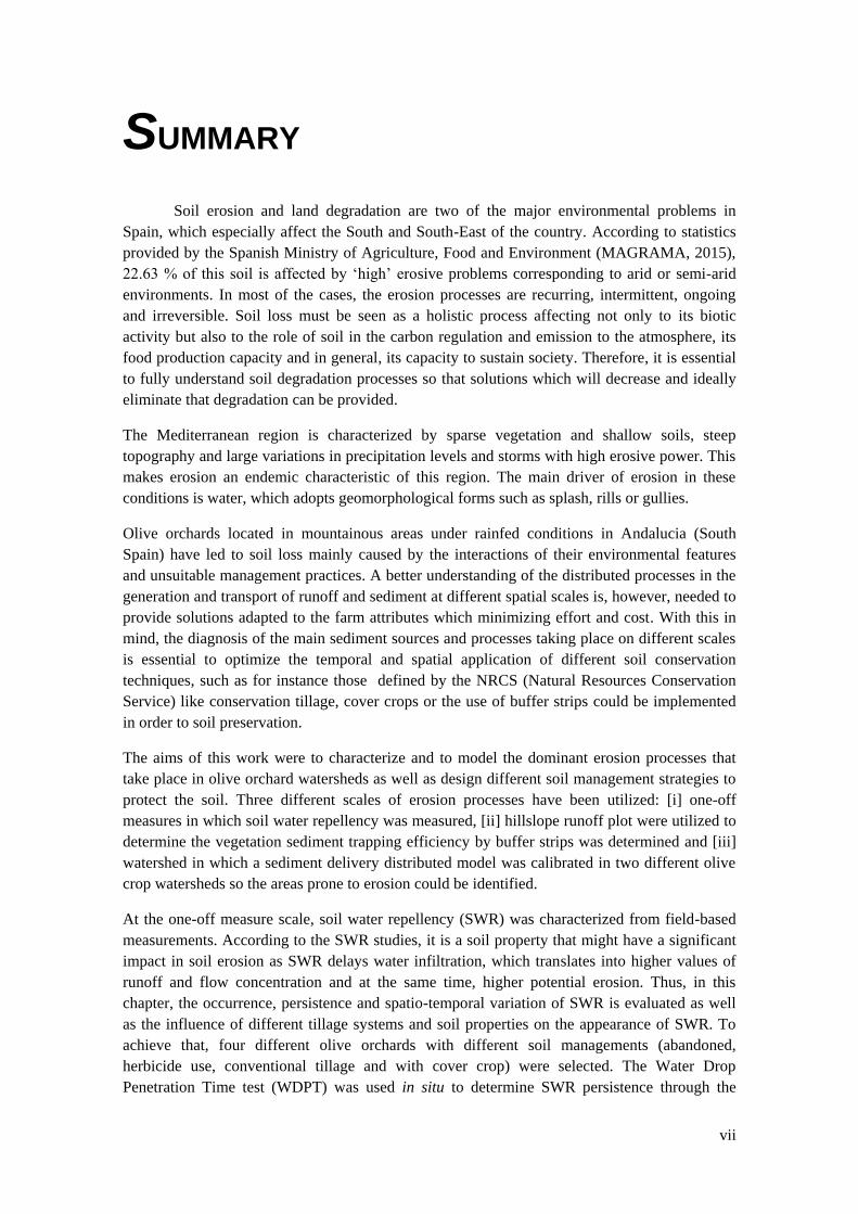
Soil erosion and land degradation are two of the major environmental problems in
Spain, which especially affect the South and South-East of the country. According to statistics
provided by the Spanish Ministry of Agriculture, Food and Environment (MAGRAMA, 2015),
22.63 % of this soil is affected by ‘high’ erosive problems corresponding to arid or semi-arid
environments. In most of the cases, the erosion processes are recurring, intermittent, ongoing
and irreversible. Soil loss must be seen as a holistic process affecting not only to its biotic
activity but also to the role of soil in the carbon regulation and emission to the atmosphere, its
food production capacity and in general, its capacity to sustain society. Therefore, it is essential
to fully understand soil degradation processes so that solutions which will decrease and ideally
eliminate that degradation can be provided.
The Mediterranean region is characterized by sparse vegetation and shallow soils, steep
topography and large variations in precipitation levels and storms with high erosive power. This
makes erosion an endemic characteristic of this region. The main driver of erosion in these
conditions is water, which adopts geomorphological forms such as splash, rills or gullies.
Olive orchards located in mountainous areas under rainfed conditions in Andalucia (South
Spain) have led to soil loss mainly caused by the interactions of their environmental features
and unsuitable management practices. A better understanding of the distributed processes in the
generation and transport of runoff and sediment at different spatial scales is, however, needed to
provide solutions adapted to the farm attributes which minimizing effort and cost. With this in
mind, the diagnosis of the main sediment sources and processes taking place on different scales
is essential to optimize the temporal and spatial application of different soil conservation
techniques, such as for instance those defined by the NRCS (Natural Resources Conservation
Service) like conservation tillage, cover crops or the use of buffer strips could be implemented
in order to soil preservation.
The aims of this work were to characterize and to model the dominant erosion processes that
take place in olive orchard watersheds as well as design different soil management strategies to
protect the soil. Three different scales of erosion processes have been utilized: [i] one-off
measures in which soil water repellency was measured, [ii] hillslope runoff plot were utilized to
determine the vegetation sediment trapping efficiency by buffer strips was determined and [iii]
watershed in which a sediment delivery distributed model was calibrated in two different olive
crop watersheds so the areas prone to erosion could be identified.
At the one-off measure scale, soil water repellency (SWR) was characterized from field-based
measurements. According to the SWR studies, it is a soil property that might have a significant
impact in soil erosion as SWR delays water infiltration, which translates into higher values of
runoff and flow concentration and at the same time, higher potential erosion. Thus, in this
chapter, the occurrence, persistence and spatio-temporal variation of SWR is evaluated as well
as the influence of different tillage systems and soil properties on the appearance of SWR. To
achieve that, four different olive orchards with different soil managements (abandoned,
herbicide use, conventional tillage and with cover crop) were selected. The Water Drop
Penetration Time test (WDPT) was used in situ to determine SWR persistence through the
viii
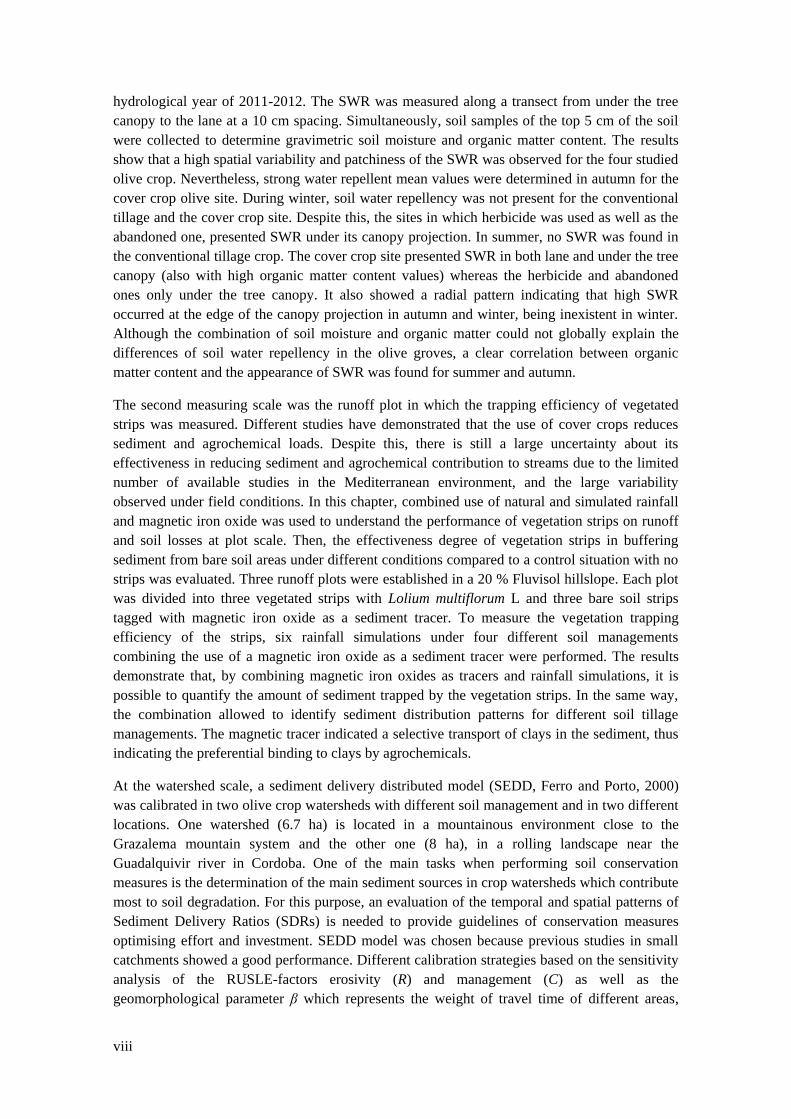
hydrological year of 2011-2012. The SWR was measured along a transect from under the tree
canopy to the lane at a 10 cm spacing. Simultaneously, soil samples of the top 5 cm of the soil
were collected to determine gravimetric soil moisture and organic matter content. The results
show that a high spatial variability and patchiness of the SWR was observed for the four studied
olive crop. Nevertheless, strong water repellent mean values were determined in autumn for the
cover crop olive site. During winter, soil water repellency was not present for the conventional
tillage and the cover crop site. Despite this, the sites in which herbicide was used as well as the
abandoned one, presented SWR under its canopy projection. In summer, no SWR was found in
the conventional tillage crop. The cover crop site presented SWR in both lane and under the tree
canopy (also with high organic matter content values) whereas the herbicide and abandoned
ones only under the tree canopy. It also showed a radial pattern indicating that high SWR
occurred at the edge of the canopy projection in autumn and winter, being inexistent in winter.
Although the combination of soil moisture and organic matter could not globally explain the
differences of soil water repellency in the olive groves, a clear correlation between organic
matter content and the appearance of SWR was found for summer and autumn.
The second measuring scale was the runoff plot in which the trapping efficiency of vegetated
strips was measured. Different studies have demonstrated that the use of cover crops reduces
sediment and agrochemical loads. Despite this, there is still a large uncertainty about its
effectiveness in reducing sediment and agrochemical contribution to streams due to the limited
number of available studies in the Mediterranean environment, and the large variability
observed under field conditions. In this chapter, combined use of natural and simulated rainfall
and magnetic iron oxide was used to understand the performance of vegetation strips on runoff
and soil losses at plot scale. Then, the effectiveness degree of vegetation strips in buffering
sediment from bare soil areas under different conditions compared to a control situation with no
strips was evaluated. Three runoff plots were established in a 20 % Fluvisol hillslope. Each plot
was divided into three vegetated strips with Lolium multiflorum L and three bare soil strips
tagged with magnetic iron oxide as a sediment tracer. To measure the vegetation trapping
efficiency of the strips, six rainfall simulations under four different soil managements
combining the use of a magnetic iron oxide as a sediment tracer were performed. The results
demonstrate that, by combining magnetic iron oxides as tracers and rainfall simulations, it is
possible to quantify the amount of sediment trapped by the vegetation strips. In the same way,
the combination allowed to identify sediment distribution patterns for different soil tillage
managements. The magnetic tracer indicated a selective transport of clays in the sediment, thus
indicating the preferential binding to clays by agrochemicals.
At the watershed scale, a sediment delivery distributed model (SEDD, Ferro and Porto, 2000)
was calibrated in two olive crop watersheds with different soil management and in two different
locations. One watershed (6.7 ha) is located in a mountainous environment close to the
Grazalema mountain system and the other one (8 ha), in a rolling landscape near the
Guadalquivir river in Cordoba. One of the main tasks when performing soil conservation
measures is the determination of the main sediment sources in crop watersheds which contribute
most to soil degradation. For this purpose, an evaluation of the temporal and spatial patterns of
Sediment Delivery Ratios (SDRs) is needed to provide guidelines of conservation measures
optimising effort and investment. SEDD model was chosen because previous studies in small
catchments showed a good performance. Different calibration strategies based on the sensitivity
analysis of the RUSLE-factors erosivity (R) and management (C) as well as the
geomorphological parameter β which represents the weight of travel time of different areas,

ix
were explored. The results show that, by using SEDD model, the areas (known as
geomorphological units) prone to erosion can be identified. The model calibration allowed
proposing a new calibration technique based on the analysis of the regions of the exponential
function determining SDR when high soil losses events are recorded in the dataset. This new
calibration allows the implementation of different values of the beta value so SDR can be
calculated with more accuracy.

x
xi
RESUMEN
La erosión y degradación del suelo son dos de los mayores problemas ambientales en
España, los cuales afectan principalmente el Este y Sudeste Peninsular. De hecho, el 22.63 % de
este suelo se ve afectado por problemas relacionados con altas erosividades de acuerdo con las
estadísticas del Ministerio de Agricultura, Alimentación y Medio Ambiente (MAGRAMA,
2015), y que se corresponde con ambientes áridos o semiáridos. En la mayoría de los casos, los
procesos erosivos son recurrentes, intermitentes, continuos e irreversibles. Es por esto por lo
que la pérdida de suelo debe ser vista como un proceso holístico que afecta no sólo a la
actividad biótica sino también al papel del suelo como regulador de las emisiones de CO2 a la
atmósfera, como capacidad productiva de alimentos y, en general, su capacidad como
sostenedor de la sociedad. De esta forma, es esencial el profundo entendimiento de los procesos
de degradación del suelo para que se puedan aportar soluciones que harán que esa degradación
pueda verse reducida sino eliminada.
La región Mediterránea se caracteriza por tener una alta variabilidad en la precipitación, así
como eventos con un alto poder erosivo, escasa vegetación, topografías accidentadas y suelos
poco profundos que hace de la erosión una característica endémica de la región. El vehículo
para el transporte de sedimento en este ambiente Mediterráneo es el agua, siendo la lluvia y la
escorrentía las fuerzas motoras para la entrega de sedimentos.
Los olivares situados en áreas montañosas y en condiciones de riego en Andalucía tienen el
agravante de la pérdida de suelo causada por la interacción de operaciones inapropiadas de
manejo de suelo, así como la no existencia de prácticas de conservación de suelo. Sin embargo,
y con la finalidad de proveer soluciones adaptadas a los atributos de las cuencas que minimicen
esfuerzo y tiempo, es necesario un mayor entendimiento de los procesos distribuidos en la
generación y transporte de escorrentía y sedimento a diferentes escalas espaciales. Con esto en
mente, se deduce la importancia del diagnóstico de las principales fuentes de sedimento y los
procesos que se dan a diferentes escalas con el fin de optimizar las aplicaciones temporales y
espaciales de las diferentes técnicas de conservación, como por ejemplo aquellas definidas por
el NRCS (Natural Resources Conservation Service) como el manejo de conservación, el uso de
cubiertas o bandas de vegetación.
La hipótesis inicial de este trabajo es que es posible identificar los procesos hidrológicos y/o
erosivos dominantes a distintas escalas espaciales utilizando medidas y modelos para un
diagnóstico apropiado del problema que proporcione soluciones de manejo que minimicen el
esfuerzo y la inversión. Para ello se determinaron tres escalas de procesos de erosión en este
trabajo: [i] medidas puntuales en las que se ha medido hidrofobicidad, [ii] parcelas de
escorrentía a escala de ladera en las que se determinó la eficiencia de atrape por bandas de
cubierta, [iii] cuencas olivareras en las que se calibró un modelo distribuido de sedimento en
dos cuencas olivareras diferentes en las que se delimitaron las áreas más susceptibles a la
erosión.
A escala de medida puntual, la hidrofobicidad (SWR) se caracterizó a partir de medidas en
campo. De acuerdo con los estudios, la SWR es una propiedad de los suelos que puede tener un
impacto significativo en la erosión del suelo dado que retrasa el tiempo de infiltración,
xii
traduciéndose en altos valores de escorrentía y concentración de flujo y, a su vez, en una mayor
erosión potencial. De esta forma, en este capítulo, la ocurrencia, persistencia y variación
espacio-temporal de la SWR se valúan, así como la influencia de los diferentes sistemas de
manejo y propiedades del suelo en la aparición de la SWR. Para conseguir esto, se
seleccionaron cuatro olivares con cuatro manejos de suelo distinto (abandonado, uso de
herbicidas, laboreo convencional y uso de cubierta). El Water Drop Penetration Time test
(WDPT) se usó in situ para determinar la persistencia de la SWR a lo largo del año hidrológico
2011-2012. La SWR se midió a lo largo de un transecto desde el área debajo de la copa hasta la
calle a un intervalo de 10 cm. Simultáneamente a las medidas de SWR, se recogieron muestras
de suelo de los primeros 5 cm para determinar humedad gravimétrica y contenido de materia
orgánica. Los resultados del capítulo presentan una alta variabilidad espacial de la SWR en los
cuatro olivares estudiados. Sin embargo, valores medios de hidrofobicidad elevados se midieron
en otoño en el olivar con cubierta vegetal. Durante el invierno, la hidrofobicidad no estuvo
presente en el olivar con laboreo convencional ni en el olivar con cubierta. A pesar de esto, el
olivar en el que hubo uso de herbicida así como el abandonado, presentaron SWR debajo de la
copa. En verano no se encontró SWR en el olivar con laboreo convencional. El olivar con
cubierta vegetal presentó SWR tanto en la calle como en el área debajo de la copa (coincidiendo
con valores elevados de materia orgánica), mientras que el olivar con uso de herbicida y el
abandonado sólo presentaron SWR en el área debajo de la copa. En este último además se
aprecia una distribución radial de la SWR indicando que ocurría en el borde del área debajo de
la copa en otoño e invierno, desapareciendo en invierno. A pesar de que la combinación de
humedad y contenido de materia orgánica en el suelo no explicaron en totalidad las diferencias
de SWR en los olivares estudiados, se encontró una correlación clara entre el contenido de
materia orgánica y la aparición de SWR en verano y otoño.
La segunda escala de medida es la parcela de escorrentía en la que evaluó la eficiencia de atrape
de las bandas de cubierta. Diversos estudios han demostrado que, el uso de las bandas de
cubierta reduce la carga de sedimento y agroquímicos al medio ambiente. A pesar de esto,
todavía existe una gran incertidumbre acerca de su grado de efectividad a la hora de reducir la
contribución de sedimentos y carga agroquímica a cursos de agua debido, principalmente, al
número limitado de estudios en ambiente Mediterráneo así como a la alta variabilidad observada
en condiciones de campo. En este capítulo se combinan dos técnicas: lluvia natural y simulada,
con trazadores de óxido de magnético con el fin de entender el rendimiento de las bandas de
cubierta en la reducción de la escorrentía y atrape de sedimentos a escala de parcela bajo
distintos manejos de suelo. Se establecieron tres parcelas de escorrentía en una ladera de
Fluvisol con 20 % de pendiente. Cada parcela se dividió en tres bandas de cubierta (Lolium
multiflorum L) y tres bandas de suelo desnudo marcado con óxido magnético como trazador de
sedimento. Para medir la eficiencia de atrape por parte de las bandas, se llevaron a cabo seis
simulaciones de lluvia con cuatro manejos de suelo distinto en los que se combinó el uso de
óxido magnético como trazador. Los resultados muestran que, mediante el uso combinado de
óxidos magnéticos como trazadores de sedimento y las simulaciones de lluvia, es posible
cuantificar la cantidad de sedimento atrapado por las bandas de cubierta. Esta combinación
permitió identificar patrones de distribución de sedimento bajo distintos manejos de suelo. El
trazador magnético indicó selectividad en el transporte de arcillas en el sedimento, indicando de
esta forma la preferencia de adhesión de los agroquímicos por las arcillas.
A escala de cuenca, se calibró el modelo distribuido de entrega de sedimentos (SEDD, Ferro y
Porto, 2000) en dos cuencas olivareras con diferentes manejos de suelo y situadas en dos
xiii
localidades distintas. Una de las cuencas (6.7 ha) está situada en ambiente montañoso cerca de
la sierra de Grazalema, la otra cuenca (8 ha) se localiza en el paisaje ondulado de la campiña del
río Guadalquivir a su paso por Córdoba. Una de las tareas más importantes a la hora de poner en
práctica medidas de conservación de suelo, es la determinación de las principales fuentes y
sumideros en las cuencas con cultivos. Para este propósito es necesaria la evaluación temporal y
espacial de los coeficientes de entrega de sedimento. Una vez evaluados a estas escalas, es más
sencillo proveer manuales con medidas de conservación, optimizando de esta forma esfuerzo e
inversión. Se eligió el modelo SEDD porque estudios previos en pequeñas cuencas demostraron
su buen rendimiento. Se exploraron diferentes estrategias de calibración basadas, por una parte,
en el análisis de sensibilidad de los factores de erosividad de RUSLE (R) y manejo (C), así
como en el parámetro geomorfológico β el cual representa los pesos de los tiempos de viaje de
las diferentes unidades geomorfológicas en las que se dividen las cuencas. Los resultados del
capítulo muestran que, mediante el uso del modelo SEDD, las áreas más susceptibles a la
erosión pueden ser determinadas e identificadas. La calibración del mismo permitió proponer
una nueva estrategia de calibración, basada en el análisis de las regiones de la función
exponencial que determina la entrega de sedimentos cuando en el conjunto de datos se dan
eventos con altas tasas de pérdida de suelo. Esta nueva calibración permite la implementación
de diferentes valores de β para, de esta forma, calcular los valores del coeficiente de entrega de
sedimentos con más exactitud.

xiv
Chapter 1: Introduction
1
Chapter 1
Introduction
‘All civilization is basically dependent upon natural resources. All natural resources…are soil
or derivatives of soil. Farms, ranges, crops and livestock, forests, irrigation water, and even
water power resolve themselves into questions of soil. Soil is therefore the basic natural
resource’.
Aldo Leopold (1887-1948)

Distributed processes in the runoff and sediment generation and transport in olive groves at different scales
2
Chapter 1: Introduction
3
Erosion is an inclusive term for the detachment and removal of soil and rock by the
action of running water, wind, waves, flowing ice and mass movement (Selby, 2005). In terms
of Geomorphology, it is a normal aspect of landscape development but it is only the dominant
process of denudation in some parts of the world.
According to the Pan European Soil Erosion Risk Assessment –PESERA–(2003), soil erosion
by water is one of the most widespread forms of soil degradation in Europe, affecting an
estimated 105 million ha, or 17 % of Europe’s total land area. The Mediterranean region
(defined here as those countries located in the South of Europe) is subjected to long dry periods
followed by intense rainfall. Those two characteristics plus its topography and soil generalities
(usually low in humus, biological activity, N, P, slow formation and thin) and unsuitable
management, makes it a region prone to erosion.
Spain, with a total surface of 504.645 km2 presents the largest area with high erosion risk
PESERA- (2003) mainly concentrated in the South and West (which is translated in the 44 % of
the territory). The increase of erosion in the region has its origin not only in the rain and its
intensities but in the deforestation, agriculture and cattle breeding that has been happening since
Neolithic times (García-Ruiz, 2010).
Among all crops grown in Spain, olive is the most important one. Furthermore, at the
Mediterranean basin scale, olive is the most representative crop with a total of 8.5 million ha
(FAOSTAT, 2012). At the national scale, olive crop represents 2.5 million ha of which 1.5 M ha
is given in Andalucía (Southern Spain) occupying 17 % of the Andalusian surface. As Gómez et
al., (2005) pointed out in a review on water erosion in olive orchards in Andalusia, the broad
extension of this crop makes any environmental question happening in the system a serious
environmental issue. One of the main characteristics which determines this crop in Andalucía is
that more than half of the cultivated hectares (999.390 ha) are located in mountainous areas and
under rainfed conditions (INE, 2009). These olive crops in steep areas have the aggravating
circumstance of soil loss as an inherent risk to the system. In a study carried out by
Vanwalleghem et al., (2011) the results showed that olive crops located in a mountainous areas
in Andalucía (Southern Spain) have lost in average between 29 and 47 t ha-1 yr-1 since the
establishment of this crop in the late XVIII early XIX centuries. Currently this soil loss is
mainly caused by erosion resulting from the use of herbicides to keep bare soil and intensive
soil management.
Soil loss experimental data were mainly carried out on runoff plot experiments. In most of
studies, the objective was to compare the effects of different management systems such as no
tillage (Gómez et al., 1999, 2004, 2009; Francia et al., 2000), cover crop strips between tree
rows (Gómez et al., 2003,2011; Arroyo et a., 2004; Milgroom et al., 2005; Hernández et al.,
2005), conventional tillage (Gómez et al., 2009, 2011; Palese et al., 2011; Lozano et al., 2014)
or herbicide use (Franco and Calatrava, 2012). Despite the amount of runoff plot scale studies
(almost all using the USLE or its revised version for computing soil losses), a bias towards high
soil losses is apparent as none of them took into account the deposition within the watershed
(Gómez et al., 2005). A better understanding of the distributed processes in the generation and
transport of runoff and sediment at different spatial scales is needed to plan economical and
efficient control measures of erosion. Up to 2009, when Taguas et al., 2009 presented their work
on watershed scale soil loss modeling validated against experimental data, little research was
carried out to study runoff responses and soil loss at the small catchment or catchment scale.
Distributed processes in the runoff and sediment generation and transport in olive groves at different scales
4
One of the biggest challenges to which conservation agriculture faces nowadays is the
integrated study at different scales of the erosive processes and sediment transport. The
following extract from the USDA report from 1928 represents the start of the modern Soil
Conservation publications. Soil erosion and soil-related environmental problems in the US
agriculture began to have interest to farmers and thus, to researchers and policy makers
(Renschler and Harbor, 2000) in the late XIX century. It was in these set of publications in
which the ‘wasting areas’ (described as areas with sheet erosion) were geomorphological
described.
…'Removal of forest growth, grass and shrubs and breaking the ground surface by cultivation,
the trampling of livestock, etc. accentuate erosion to a degree far beyond that taking place
under average natural conditions, especially on those soils that are peculiarly susceptible to
rainwash’.
- H.H. Bennet and W.R. Chapline (1928), Soil erosion: a national menace.
During the 60’s and 70’s watershed modelling studies was generalized. For instance, the work
of Onstad and Foster (1975) on erosion modelling on Treynor watershed marked a breaking
point in erosion studies. During the 90’s and up to now the soil deposition studies at this scale
was generalized due to new sediment dating techniques at watershed scale (mainly
radionuclides in a 18.5 % as Guzmán, 2011 pointed out) such as 137Cs (Martz and de Jong.,
1991), or 210Pb (Walling et al., 1999) and at hillslope scale (Wallbrink and Murray, 1993). In
this way, erosion generating processes (detachment and transport) were being attempted at
different scales.
This PhD thesis is focused on throwing light to the study of different transport processes and
sediment generation in olive orchards at different spatial scales. They have been chosen
because; despite decades of research they are still relatively poorly understood. Improvement on
the understanding of these processes might help to the development of better soil conservation
strategies in olive growing areas, as well as providing a fruitful environment for PhD training.
This training purpose was reinforced by the fact that it was developed within the frame of a
research project 'Caracterización y efecto sobre la exportación total, de las fuentes y sumideros
de escorrentía, sedimento y carbono en cuencas agrícolas en ambientes mediterráneos'. AGL
2009 (12936-C03-01). The three topics have been: [1] soil water repellency as local phenomena
at point scale, [2] sediment trapping by cover crop strips at runoff plot scale and [3] modeling of
water erosion at small watershed scale.
1.1. One-off measure scale
Within the hydrology field and as an example of one-off measure, one of the aspects which
became of interest from 1960-1969 was soil water repellency. Soil water repellency is defined
by some authors as a soil property that might appear in most soil types which reduces its
infiltration capacity and it might have important hydrological and geomorphological
consequences (Jordán et al., 2010). During this decade and as pointed out by the water
repellency overview done by De Bano (2000) a wide range of papers concerning soil water
repellency started to surge (most of them published in the first international conference at
Riverside, CA).
Chapter 1: Introduction
5
At the same time, Letey et al., (1962) developed the contact angle methodology in order to
characterize soil water repellency. It was during the 70’s when the interest of soil water
repellency attracted worldwide scientists and research was conducted on fire-induced water
repellency (De Bano et al., 1976), water harvesting (Cooley et al., 1975), water repellency
characterization (Watson and Letey, 1970) and soil water movement (De Bano, 1975).
The occurrence of SWR is determined by the type and quantity of hydrophobic substances in
the soil, all of them with a biological origin: waxes and resins (DeBano. 1981), root exudates
(Doerr et al., 1998), fungi or microorganisms (Savage et al., 1969), or directly from
decomposing organic matter (McGhie and Posner, 1981).Other factors such as soil temperature
(Savage, 1974), soil texture (Blackwell, 1993) and soil moisture (Dekker and Ritsema, 1996)
have an effect on its persistence (a review of these factors can be found in Doerr et al., 2000).
This is indicating that SWR is only found under soils with a certain type of properties such as a
sandy texture or a certain level of organic matter and, what it is more, not only organic matter
but certain substances of it. So if the soil does not match those properties, it will be exerting of
developing SWR.
Nonetheless, soil water repellency measurements have been performed under extreme
soil/vegetation situations. In fact, it is still mainly focused on forest soils with pine and
eucalyptus (Leighton-Boyce et al., 2005) in which soils become hydrophobic due to oleos
substances from the vegetation (see for instance the work carried out by Doerr et al., 2003 in
Portuguese watersheds or Bodí et al., 2011 under Mediterranean plant species type).
To our knowledge, most of those situations in which soil water repellency have been measured
are not representing what could happen under typical crop conditions. Despite the scarce
measurements performed under agricultural land, soil water repellency is still considered by
some authors an inherent soil property and thus it can be extrapolated to all soils even under a
broad range of cropping systems (Blanco-Canqui and Lal, 2009).
Soil water repellence is measured one-off through the Water Drop Penetration Time (WDPT)
test (Letey, 1969) or the MED (Molarity of Ethanol Droplet) for its intensity (Watson and
Letey, 1970). WDPT is a test based on placing a water drop (0.05 mL in this case), using a
syringe, on a soil surface and recording the time that it takes for the drop to break the surface
tension and infiltrate. The more it takes for a water drop to infiltrate (>5 s) the more
hydrophobic the soil is considered and so the more prone to generate surface runoff. Despite
both measures being at the one-off scale, Doerr et al., (2003) in a Portuguese watershed scaled-
up the measures from the point scale-plot scale-catchment scale finding reduced correspondence
between scales. In fact, their work shows that, due to catchment sinks (translated as
reinfiltration processes) SWR diminishes at a larger scale than the hillslope plot.
Although SWR has been described as a soil property (Doerr et al., 2000), meaning that all soils
have it in common, it has been reported to be absent under agricultural land. For instance, in a
work carried out by Cerdà and Doerr (2007) examining six land uses (two of them crops: orange
and olives) under calcareous soil and under dry and wet season, found that water repellence was
absent. In the case of horticultural crops, in which soil properties such as organic matter content
or soil moisture content (two of the main factors contributing to the appearance of soil water
repellency) changes depending on the season and tillage systems, little research has been done.
Following this reasoning, SWR might not be an important runoff and water erosion driver under
tree crop lands.
Distributed processes in the runoff and sediment generation and transport in olive groves at different scales
6
However, Ziogas et al., (2005) in Northeast Greece found that under the olive tree canopies, the
soil (sandy loamy), could be extremely water repellent during the winter season. This
information contradicts with several studies on infiltration rates within olive orchards,
summarized in Romero et al., (2007) in which high infiltration rates are found under the olive
tree canopies. The contradictory information and the fact that olive is the main crop in the
Mediterranean region, make a point on measuring SWR under olive crops in Spain under
different soil managements. If exists, it aims to be one of the distributed processes at the
hydrological level which might contribute to the sediment generation and transport, thus being a
point of support when determining sources of runon and runoff in olive crops.
1.2. Sediment trapping by cover crop strips at hillslope scale
Once understood runon and runoff areas within the olive crop, sediment tracers were used to
describe and quantify the sediment transport in plots located in hillslopes under different soil
management practices commonly applied in olive commercial farms, among others, the impact
of cover crops.
Sediment tracing techniques have been in used since the 80’s in order to study the precedence of
the sediment in maritime transport processes. The ‘tracing’ technique of the sediment comprises
tagging the sediment which is collected at the watershed outlet with any tracer and compared
the signal with the watershed soil.
According to the review by Guzmán (2011), as no single tracer technique fulfills all the
requirements of an ideal erosion tracer proposed by Zhang et al., (2001), there are different
sediment tracers used in different sediment tracer studies. Tracer types are divided in
radionuclides (derived from nuclear techniques), fingerprinting techniques, rare earth elements
and magnetic tracers (Guzmán 2011). One of the sediment tracing techniques started up in the
last years is related to the use of the magnetic iron oxide (Fe3O4) as a sediment tracer (Guzmán
et al., 2010). The tracer is a synthetic magnetic iron oxide commercially available as Bayferrox
® 318 M and used as a black powder pigment. The main characteristic is that its particles bind
together with the soil particles thus being able to trace the sediment movement in a Lagrangian
way. Once the soil is tagged with the tracer, the sediment movement can be tracked and mapped
using a MS2D® field loop calibration by measuring the changes in tracer concentrations in soil
after the tagging. Mass magnetic susceptibility in the laboratory is then measured with the
MS2B® Dual Frequency Sensor at 0.465 kHz with accuracy to ±1 %. For top soil determination
of magnetic susceptibility, non-destructive measurements are made using a Bartington MS2D®
field loop, which operates at a frequency of 0.958 kHz (Dearing, 1999). A mixing model
developed by Guzmán et al. (2013) was used to determine the sources of the sediment within an
olive orchard. In fact, in the work developed by Guzmán (2011) at the plot scale in an olive
watershed in Southern Spain, the combined of rainfall simulations-natural rainfall-magnetic iron
oxide as a tracer resulted in the determination of the erosion areas prone to splash and interrill.
In soil conservation studies, one of the measures proposed is the use of vegetation strips
(Giráldez and Gómez, 2009) as a strategy to mitigate soil loss and retain sediment. Grass strips
are described as permanent vegetation or part of the crop rotation cycle which are set out along
contour lines, separated by strips of arable land (van Dijk et al., 1996). They work hydraulically
increasing roughness to reduce flow velocity and promoting sediment deposition as well as
Chapter 1: Introduction
7
adsorption by the vegetation. In our experiment, vegetation strips would be a complementary
use to conventional tillage that, combined with the use of sediment tracers and rainfall
simulations at the hillslope scale, would help to identify on a first stage which is the origin of
the sediment trapped in the strips, and on a second stage, the amount of sediment retained in the
strips. However, the combination of experimental and modelling analyses indicate that a broad
range of efficiency degrees of grass strips in sediment trapping and in filtering are expected.
In the Mediterranean region little research has been performed on the impact and efficiency of
vegetation strips in order to reduce runoff and soil losses and, thus, trapping sediment. For
instance, Raya et al., (2006) in runoff plots located in a mountainous area in Southern Spain
with almond tress tested three different plant-cover strips: barley, thyme and lentils. Their work
demonstrated that barley cover crop was the most effective in reducing soil losses and runoff
when compared to bare soil. At the same time, Durán-Zuazo et al., (2009) in the same region
but with different crop (olives) also found that mean annual soil erosion and runoff was reduced
by combining no tillage soil management and barley cover crop strip. This indicates that more
information in order to full the information niche regarding vegetation trapping efficiency in
Mediterranean areas is of need.
1.3. Watershed scale
The last scale in which transport processes are performed is the watershed scale. Watershed
scale modeling has been carried out since the end of the XIX century with the first studies about
watershed hydrological responses to events (James Mulvaney, in 1851, showed how peak flows
can be estimated from average rainfall intensity and catchment area). Despite the advances
performed in rainfall-runoff modeling at this scale from the 70’s up to now, Freezer (1978)
stated that ‘we would never be able to model the complexity of real world hillslope hydrology,
and that the divergences between model and reality would always remain substantial’.
One of the progresses which allowed the improvement of the modeling of hydrological
processes at this scale is the use of the Geographical Information Systems (GIS). The routine
implementation to determine watershed travel times, the possibility to obtain DEM and work
with them and even the computing of equations such as RUSLE (Renard et al., 1997), allowed
the enhancement of the techniques when generating runoff or soil loss values. Research
performed during the last 50 years developed mathematical models in order to predict sediment
production at different spatial and temporal scales, as well as performed specific monitoring of
the different erosive processes in different regions of the world (a review of the different models
applied in soil erosion studies can be found in Merrit et al., 2003). Erosion models are useful for
understanding hydrological processes, simple parametric approximations such as USLE
(Universal Soil Loss Equation; Wischmeier and Smith, 1978) or its revised version RUSLE
(Renard et al., 1997) are commonly used for evaluating risk of soil erosion all around the world.
In order to understand different runoff scenarios for soil management decision-making, water
conservation plans or climate change information on soil management, soil modeling is then of
need. It is important to calibrate those models in a complex environmental context derived from
climate, soil, topographic, land use and soil management variability. It is then necessary
appropriate calibration techniques.

Distributed processes in the runoff and sediment generation and transport in olive groves at different scales
8
Within the approach to understand the origin of the sediment (or its sources) and reinforcing the
information that can be obtained from the hillslope scale with the magnetic tracers, the division
of the watersheds into geomorphological units has been one of the key points for the
implementation of soil and water conservation strategies. A geomorphological unit is defined as
an area with a defined aspect, length and steepness (Ferro and Porto, 2000). This division of the
watershed into geomorphological units allow, on the one hand to the identification of areas
more prone to soil erosion and thus sediment generation and transport. On the other hand and at
a more agronomic level, knowing the areas prone to soil erosion allow a more specific
establishment of soil and water conservation practices.
Chapter 2: Assessment of soil water repellency in olive groves from Spain
9
Chapter 2
Assessment of soil water repellency
in olive groves from Spain
Part of the results of this chapter has been presented as a communication in:
European Geoscience Union, EGU (2012):
Burguet, M., Taguas, E.V., Gómez, J.A.: Exploring the importance of hydrophobicity in
the hydrologic cycle of olive groves in Spain. European Geoscience Union, EGU, 2012
‘To be a successful farmer one must first know the nature of soil’
Xenophon (c. 430-354 BC)

Distributed processes in the runoff and sediment generation and transport in olive groves at different scales
10
Chapter 2: Assessment of soil water repellency in olive groves from Spain
11
Resumen
La hidrofobicidad (SWR) ha sido medida en diferentes suelos, manejos de suelo y
regiones del mundo, y en particular en zonas forestales después de incendios. A pesar de ello, la
comprensión de la aparición o no de esta variable en suelos agrícolas todavía es limitada. Este
estudio presenta la caracterización de la SWR medida en campo y en diferentes olivares (Olea
europaea L.) en España con diferentes condiciones ambientales y manejos. Los objetivos
principales de este trabajo fueron: [1] evaluar la ocurrencia y persistencia de la SWR bajo
distintos manejos de suelo en olivar, [2] explorar sus características espacio-temporales, [3]
explorar la influencia de los distintos sistemas de laboreo y propiedades del suelo como el
contenido de materia orgánica y la humedad del suelo en la persistencia de la SWR en el que es
el mayor cultivo de la cuenca Mediterránea. Para ello se seleccionaron cuatro olivares con
distintos manejos de suelo (abandonado, laboreo convencional, uso de herbicida y cubierta
vegetal) en Córdoba (Sur de España) y Valencia (Este de España). El Water Drop Penetration
Time test (WDPT) se utilizó para evaluar in situ los valores de SWR en tres estaciones: otoño,
invierno y verano. Las medidas se llevaron a cabo en el año hidrológico 2011-2012 en dos áreas
para cada uno de los olivares seleccionados: en el suelo bajo copa y en las calles. Los valores
del WDPT resultaron ser altamente variables en los cuatro olivares estudiados. La SWR estuvo
ausente en el olivar con laboreo convencional siendo además el olivar con el contenido de
materia orgánica más bajo. Los valores más elevados se midieron en verano debajo de las copas
(WDPT= 610 s) y en otoño en las calles (WDPT= 468 s). A pesar de esto, no se encontró un
patrón estable en la aparición/desaparición de la SWR en relación a los cambios estacionales o
los diferentes manejos de suelo. La SWR estuvo más relacionada con el contenido de materia
orgánica del suelo y eventos de lluvia significativos en los meses previos a las mediciones en
campo. Los resultados ilustran que la importancia hidrológica de la SWR es muy variable y
puede que no sea importante a la hora de desencadenar procesos de escorrentía en el olivar.
Palabras clave: hidrofobicidad, olivar, hidrología, manejo de suelo, materia orgánica.
Distributed processes in the runoff and sediment generation and transport in olive groves at different scales
12
Abstract
Soil water repellency (SWR) has been reported under different soils, land uses and
regions of the world, particularly in forested areas after wildfires, yet the understanding of this
variable in agricultural lands is still rather limited. This study presents the characterization from
field-based measurements of SWR in several olive groves (Olea europaea L.) in Spain under
different conditions and managements. The main objectives of this research were: [1] to
evaluate the occurrence and persistence of SWR under different soil managements in olive
groves; [2] to explore its spatio-temporal features; [3] to explore the influence of different
tillage systems and soil properties such as organic matter content and soil moisture in the
persistence of SWR in the major cropland system in the Mediterranean basin. Four different
groves with different soil management (abandoned, conventional tillage, herbicide use and
cover crop) were chosen in Cordoba (Southern Spain) and Valencia (East Spain). The Water
Drop Penetration Time test (WDPT) was used in situ to assess SWR values in three seasons:
autumn, winter and summer. Measurements were carried out for one hydrological year (2011-
20212) in two areas for each of the four groves: below (canopy) and between the tree canopies
(lanes). A high variability of WDPT values was observed in the studied olive groves. SWR was
absent for the olive grove under conventional tillage and with the lowest values of organic
matter. The highest values were found under canopies (WDPT = 610 s) in summer and on the
lanes (WDPT= 468 s) in autumn. However, there was no stable pattern with regards to seasonal
changes or different soil managements; SWR appeared more related to organic matter content
and significant rainfall events in the months prior to field measurements. The results illustrated
that the hydrological relevance of the SWR is highly variable and it might not be substantial on
triggering runoff processes in olive groves.
Keywords: soil water repellency, olive, hydrology, soil management, organic matter.
Chapter 2: Assessment of soil water repellency in olive groves from Spain
13
2.1. Introduction
Olive is the main crop in the Mediterranean region and it forms, along with wheat and wine,
what it is known as the ‘Mediterranean triad’. Mediterranean countries produce over 95% of
the world’s olive oil which has a relevant socio-economic impact. The olive and olive oil
production is also resulting in environmental impacts. High soil erosion rates and the diffusion
of water pollution, among others, are serious degradation risks commonly associated with the
hydrological processes in olive groves (Goméz-Limón et al., 2011). The non-sustainable soil
erosion rates are mainly related to steep slopes which favours runoff generation and where,
traditionally, olives have been cultivated. In addition to the topography and microtopography,
spatial patterns derived from the traffic, management and the influence of trees cause variations
of soil physical properties, which encourage high soil erosion rates (Gómez et al., 1999).
In this context of varying soil properties, accelerated soil erosion rates and enhanced high runoff
rates in the olive groves, SWR might have a significant impact as delays water infiltration,
which translates into higher values of runoff and flow concentration (Doerr et al., 2000;
Shakesby et al., 2000) and at the same time, higher potential erosion.
The occurrence of SWR is determined by the type and quantity of hydrophobic substances in
the soil, all of them with a biological origin: waxes and resins (DeBano. 1981), root exudates
(Doerr et al., 1998), fungi or microorganisms (Savage et al., 1969), or directly from
decomposing organic matter (McGhie and Posner, 1981).
Other factors such as soil temperature, soil texture and soil moisture have an effect on its
persistence (a review of these factors can be found in Doerr et al., (2000)). Many of these
factors are present in olive groves and can result in SWR occurrence in these crops. However, as
far as we are concerned, no measurements have been carried out on olive plantations until now.
Moreover, some of the olive production, specially the one on the floor, is not collected,
increasing the amount of oils incorporated in the soil surface. SWR can affect water infiltration
as it reduces the soil matrix infiltration rates, and can increase the macropore flow. This can
result in the reduction of the water availability for the vegetation, specially the crop. SWR also
have biological, hydrological and geomorphological implications: the reduction of water
availability translates into a severe tree stress, and as the water fluxes are more concentrated soil
erosion rates can get high. Preferential flow is also more feasible if SWR take place.
Soil water repellency is being a key topic in soil hydrology, but still mainly focused on forest
soils, although the initial research was done in agricultural sandy soils in Florida (Wander,
1949). A review done in the Web of Knowledge in September 2013 to find the studies dealing
with SWR occurrence and different croplands in the period 2000-2013, using the words
'wettability', 'soil hydrophobicity', and 'soil water repellency' resulted in 55% of the publications
in forests, 27% in croplands and 18% in grasslands.
In the case of horticultural crops, preliminary research has been carried out in organic peat soils
with irrigated potato crop in Sweden under four types of organic soils, reporting low SWR
values when low soil moisture content (Berglund and Persson, 1996). SWR has been also
studied on sandy soils in intensive irrigation potato cultivation in Suffolk, -Great Britain-
(Robinson, 1999). In this study, the author found slightly water repellent points with large
spatial variability that caused an increase in the deficit irrigation and in the scab infection of the
cultivation.
Distributed processes in the runoff and sediment generation and transport in olive groves at different scales
14
For SWR variations through time and crop-rotation systems, Keizer et al. (2007) found very
persistent values in a system of potatoes, maize and fallow in central Portugal. In this case,
spatial patterns of the studied phenomena were found in furrows and ridges. In a review of field
crops studies, Blanco-Canqui (2011) found that different soil managements orientated towards
conservation agriculture (e.g. no-tillage vs. conventional till) increased the trend towards soil
water repellency, as most of the conventional tillage soils can be classified as 'wettable' whilst
the no-tillage ones, which had higher organic matter content in the top soil, are classified as
'slightly water repellent'.
Considering Mediterranean tree crops, in Northeast Greece, Ziogas et al. (2005) measured SWR
below olive trees in a sandy soil. Their laboratory results showed that under the olive tree
canopies the soil could be extremely water repellent during the winter season. These results
seems to be contradictory with several studies on infiltration rates within olive orchards,
summarized in Romero et al. (2007), which found higher infiltration rates in the soil below olive
canopy projection. Cerdà and Doerr (2007) evaluated SWR under orange and olive groves, and
cereal crop in field surveys in Eastern Spain. No significant SWR was found at the agricultural
sites.
Under this context, a better understanding of SWR in olive groves, its extension, temporal and
seasonal changes as well as intensity in relation to soil management and cropping systems
seems fundamental to evaluate its implication in the overall hydrologic response of olive
groves, and may be used to improve water management and irrigation practices in olive groves.
This study was conceived with aims to: i) evaluate the occurrence and persistence of SWR
under different soil managements in olive groves; ii) explore its spatio-temporal features as well
iii) to explore the influence of different tillage systems and soil properties such as organic
matter content and soil moisture in the persistence of SWR in the major cropland system in the
Mediterranean basin.
2.2. Study site and available data
This study was carried out in four olive groves in Southern and Eastern Spain (Fig. 2.1).
Three were located in the province of Cordoba (Southern Spain), with different soil
managements (Figure 2.2, Table 2.1): permanent cover crop periodically mowed in an organic
grove (CC), conventional tillage allowing cover crop in the lanes and bare soil using herbicide
under the olive canopy (CT), and weed growing controlled with periodic applications of
herbicide (H). An olive grove abandoned forty years ago was also surveyed in Valencia
province, Eastern Spain (AB). In this last grove, the soil was partially covered by natural
vegetation among the olive trees, dominated by rosemary (Rosmarinus officinalis L.), thyme
(Thymus vulgaris L.), kermes oak (Quercus coccifera L.) and maritime pine (Pinus pinaster L.).
This abandoned olive grove show the impact of the vegetation and soil recovery after the land
abandonment.
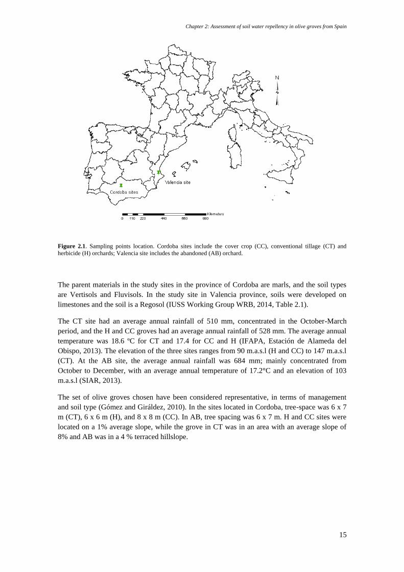
Chapter 2: Assessment of soil water repellency in olive groves from Spain
15
Figure 2.1. Sampling points location. Cordoba sites include the cover crop (CC), conventional tillage (CT) and
herbicide (H) orchards; Valencia site includes the abandoned (AB) orchard.
The parent materials in the study sites in the province of Cordoba are marls, and the soil types
are Vertisols and Fluvisols. In the study site in Valencia province, soils were developed on
limestones and the soil is a Regosol (IUSS Working Group WRB, 2014, Table 2.1).
The CT site had an average annual rainfall of 510 mm, concentrated in the October-March
period, and the H and CC groves had an average annual rainfall of 528 mm. The average annual
temperature was 18.6 ºC for CT and 17.4 for CC and H (IFAPA, Estación de Alameda del
Obispo, 2013). The elevation of the three sites ranges from 90 m.a.s.l (H and CC) to 147 m.a.s.l
(CT). At the AB site, the average annual rainfall was 684 mm; mainly concentrated from
October to December, with an average annual temperature of 17.2°C and an elevation of 103
m.a.s.l (SIAR, 2013).
The set of olive groves chosen have been considered representative, in terms of management
and soil type (Gómez and Giráldez, 2010). In the sites located in Cordoba, tree-space was 6 x 7
m (CT), 6 x 6 m (H), and 8 x 8 m (CC). In AB, tree spacing was 6 x 7 m. H and CC sites were
located on a 1% average slope, while the grove in CT was in an area with an average slope of
8% and AB was in a 4 % terraced hillslope.
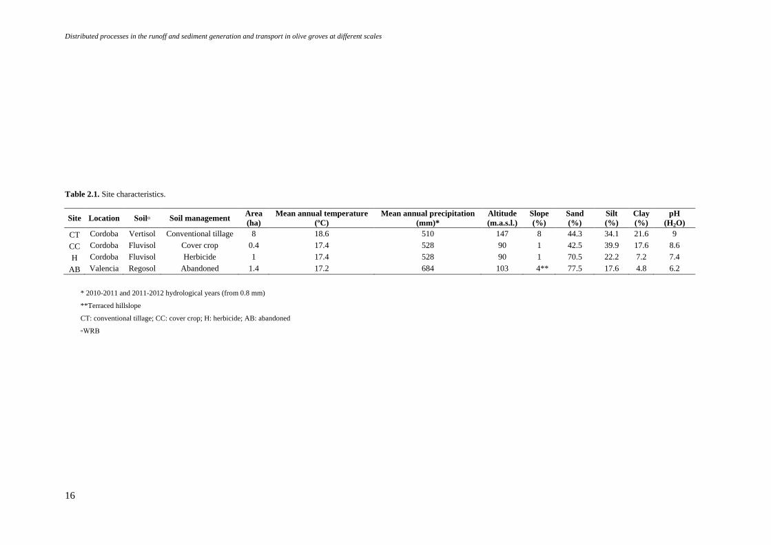
Distributed processes in the runoff and sediment generation and transport in olive groves at different scales
16
Table 2.1. Site characteristics.
Site Location Soil▫ Soil management Area
(ha)
Mean annual temperature
(ºC)
Mean annual precipitation
(mm)*
Altitude
(m.a.s.l.)
Slope
(%)
Sand
(%)
Silt
(%)
Clay
(%)
pH
(H2O)
CT Cordoba Vertisol Conventional tillage 8 18.6 510 147 8 44.3 34.1 21.6 9
CC Cordoba Fluvisol Cover crop 0.4 17.4 528 90 1 42.5 39.9 17.6 8.6
H Cordoba Fluvisol Herbicide 1 17.4 528 90 1 70.5 22.2 7.2 7.4
AB Valencia Regosol Abandoned 1.4 17.2 684 103 4** 77.5 17.6 4.8 6.2
* 2010-2011 and 2011-2012 hydrological years (from 0.8 mm)
**Terraced hillslope
CT: conventional tillage; CC: cover crop; H: herbicide; AB: abandoned
▫WRB
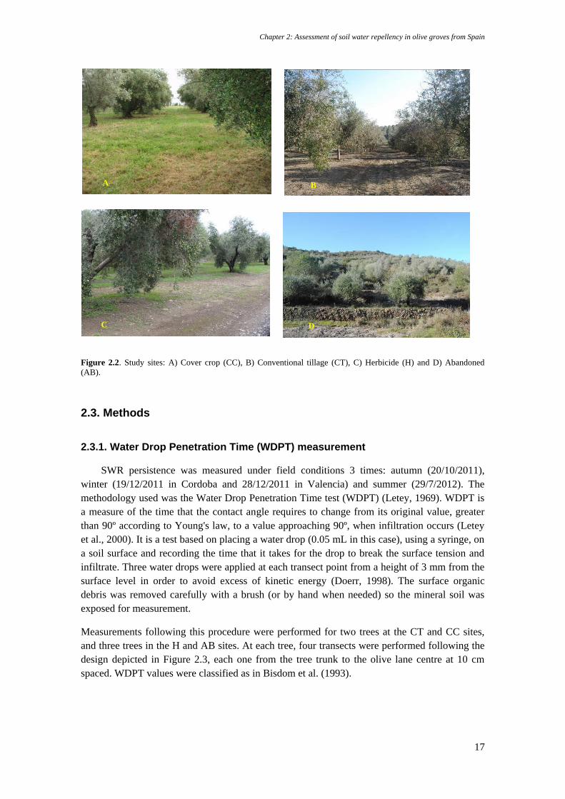
Chapter 2: Assessment of soil water repellency in olive groves from Spain
17
Figure 2.2. Study sites: A) Cover crop (CC), B) Conventional tillage (CT), C) Herbicide (H) and D) Abandoned
(AB).
2.3. Methods
2.3.1. Water Drop Penetration Time (WDPT) measurement
SWR persistence was measured under field conditions 3 times: autumn (20/10/2011),
winter (19/12/2011 in Cordoba and 28/12/2011 in Valencia) and summer (29/7/2012). The
methodology used was the Water Drop Penetration Time test (WDPT) (Letey, 1969). WDPT is
a measure of the time that the contact angle requires to change from its original value, greater
than 90º according to Young's law, to a value approaching 90º, when infiltration occurs (Letey
et al., 2000). It is a test based on placing a water drop (0.05 mL in this case), using a syringe, on
a soil surface and recording the time that it takes for the drop to break the surface tension and
infiltrate. Three water drops were applied at each transect point from a height of 3 mm from the
surface level in order to avoid excess of kinetic energy (Doerr, 1998). The surface organic
debris was removed carefully with a brush (or by hand when needed) so the mineral soil was
exposed for measurement.
Measurements following this procedure were performed for two trees at the CT and CC sites,
and three trees in the H and AB sites. At each tree, four transects were performed following the
design depicted in Figure 2.3, each one from the tree trunk to the olive lane centre at 10 cm
spaced. WDPT values were classified as in Bisdom et al. (1993).
A B
C D
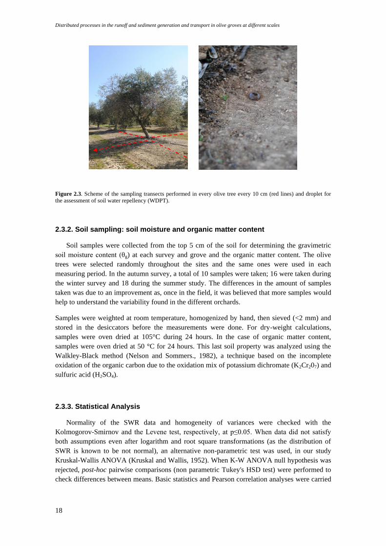
Distributed processes in the runoff and sediment generation and transport in olive groves at different scales
18
Figure 2.3. Scheme of the sampling transects performed in every olive tree every 10 cm (red lines) and droplet for
the assessment of soil water repellency (WDPT).
2.3.2. Soil sampling: soil moisture and organic matter content
Soil samples were collected from the top 5 cm of the soil for determining the gravimetric
soil moisture content (θg) at each survey and grove and the organic matter content. The olive
trees were selected randomly throughout the sites and the same ones were used in each
measuring period. In the autumn survey, a total of 10 samples were taken; 16 were taken during
the winter survey and 18 during the summer study. The differences in the amount of samples
taken was due to an improvement as, once in the field, it was believed that more samples would
help to understand the variability found in the different orchards.
Samples were weighted at room temperature, homogenized by hand, then sieved (<2 mm) and
stored in the desiccators before the measurements were done. For dry-weight calculations,
samples were oven dried at 105°C during 24 hours. In the case of organic matter content,
samples were oven dried at 50 °C for 24 hours. This last soil property was analyzed using the
Walkley-Black method (Nelson and Sommers., 1982), a technique based on the incomplete
oxidation of the organic carbon due to the oxidation mix of potassium dichromate (K2Cr207) and
sulfuric acid (H2SO4).
2.3.3. Statistical Analysis
Normality of the SWR data and homogeneity of variances were checked with the
Kolmogorov-Smirnov and the Levene test, respectively, at p≤0.05. When data did not satisfy
both assumptions even after logarithm and root square transformations (as the distribution of
SWR is known to be not normal), an alternative non-parametric test was used, in our study
Kruskal-Wallis ANOVA (Kruskal and Wallis, 1952). When K-W ANOVA null hypothesis was
rejected, post-hoc pairwise comparisons (non parametric Tukey's HSD test) were performed to
check differences between means. Basic statistics and Pearson correlation analyses were carried
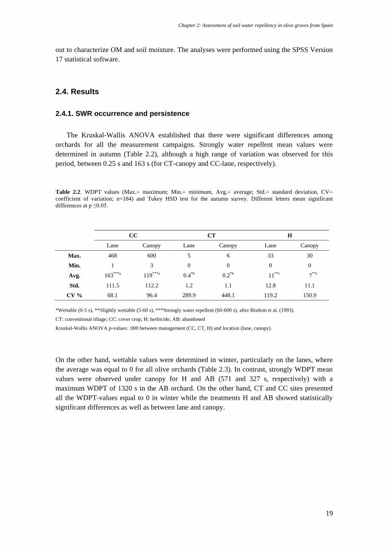
Chapter 2: Assessment of soil water repellency in olive groves from Spain
19
out to characterize OM and soil moisture. The analyses were performed using the SPSS Version
17 statistical software.
2.4. Results
2.4.1. SWR occurrence and persistence
The Kruskal-Wallis ANOVA established that there were significant differences among
orchards for all the measurement campaigns. Strongly water repellent mean values were
determined in autumn (Table 2.2), although a high range of variation was observed for this
period, between 0.25 s and 163 s (for CT-canopy and CC-lane, respectively).
Table 2.2. WDPT values (Max.= maximum; Min.= minimum, Avg.= average; Std.= standard deviation, CV=
coefficient of variation; n=184) and Tukey HSD test for the autumn survey. Different letters mean significant
differences at p ≤0.05.
CC CT H
Lane Canopy Lane Canopy Lane Canopy
Max. 468 600 5 6 33 30
Min. 1 3 0 0 0 0
Avg. 163***a 119***a 0.4*b 0.2*b 11**c 7**c
Std. 111.5 112.2 1.2 1.1 12.8 11.1
CV % 68.1 96.4 289.9 448.1 119.2 150.9
*Wettable (0-5 s), **Slightly wettable (5-60 s), ***Strongly water repellent (60-600 s), after Bisdom et al. (1993).
CT: conventional tillage; CC: cover crop; H: herbicide; AB: abandoned
Kruskal-Wallis ANOVA p-values: .000 between management (CC, CT, H) and location (lane, canopy).
On the other hand, wettable values were determined in winter, particularly on the lanes, where
the average was equal to 0 for all olive orchards (Table 2.3). In contrast, strongly WDPT mean
values were observed under canopy for H and AB (571 and 327 s, respectively) with a
maximum WDPT of 1320 s in the AB orchard. On the other hand, CT and CC sites presented
all the WDPT-values equal to 0 in winter while the treatments H and AB showed statistically
significant differences as well as between lane and canopy.

Distributed processes in the runoff and sediment generation and transport in olive groves at different scales
20
Table 2.3. WDPT values (Max.= maximum; Min.= minimum, Avg.= average; Std.= standard deviation, CV=
coefficient of variation; n=184) and Tukey HSD test for the winter survey. Different letters mean significant
differences at p ≤0.05.
*Wettable (0-5 s), **Slightly wettable (5-60 s), ***Strongly water repellent (60-600 s), after
Bisdom et al. (1993).
CT: conventional tillage; CC: cover crop; H: herbicide; AB: abandoned
Kruskal-Wallis ANOVA p-values: .000 between management (CC, CT, H) and location (lane,
canopy).
In the summer survey SWR was found both under the canopy and in the lane for CC grove
(28 and 61 seconds respectively, Table 2.4). H and AB groves only had SWR under the tree
canopy (20 and 37 seconds respectively) and wettable conditions were measured in the CT site.
There were significant differences between lane and canopy for CC, H and AB groves, and
among groves. In case of CC, SWR showed a stable pattern during autumn and summer, where
the radial patterns indicates that the highest WDPT values tended to be around the edge of the
canopy projection whilst, in winter, SWR was inexistent.
Table 2.4. WDPT values (Max. = maximum; Min.= minimum, Avg.= average; Std.= standard deviation, CV=
coefficient of variation; n=184) and Tukey HSD test for the winter survey. Different letters mean significant
differences at p ≤0.05.
CC CT H AB
Lane Canopy Lane Canopy Lane Canopy Lane Canopy
Max. 253 610 0 0 101 190 0 434
Min. 0 0 0 0 0 0 0 0
Avg. 28**a 61***a 0*d 0*d 2*c,d 20**c,d 0*b,c,d 37**b,c,d
Std. 35.4 77.6 0 0 9.0 32.7 0 60.3
CV % 128.9 126.3 - - 846.8 160.1 - 163.2
*Wettable (0-5 s), **Slightly wettable (5-60 s), ***Strongly water repellent (60-600 s), after
Bisdom et al. (1993).
CT: conventional tillage; CC: cover crop; H: herbicide; AB: abandoned
Kruskal-Wallis ANOVA p-values: .000 between management (CC, CT, H) and location (lane,
canopy).
CC CT H AB
Lane Canopy Lane Canopy Lane Canopy Lane Canopy
Max. 0 0 0 0 0 800 0 1320
Min. 0 0 0 0 0 387 0 0
Avg. 0*b 0*b 0*b 0*b 0*a,b 571***a,b 0*a,b 327***a,b
Std. 0 0 0 0 0 158.9 0 459.6
CV % - - - - - 27.8 - 140.4
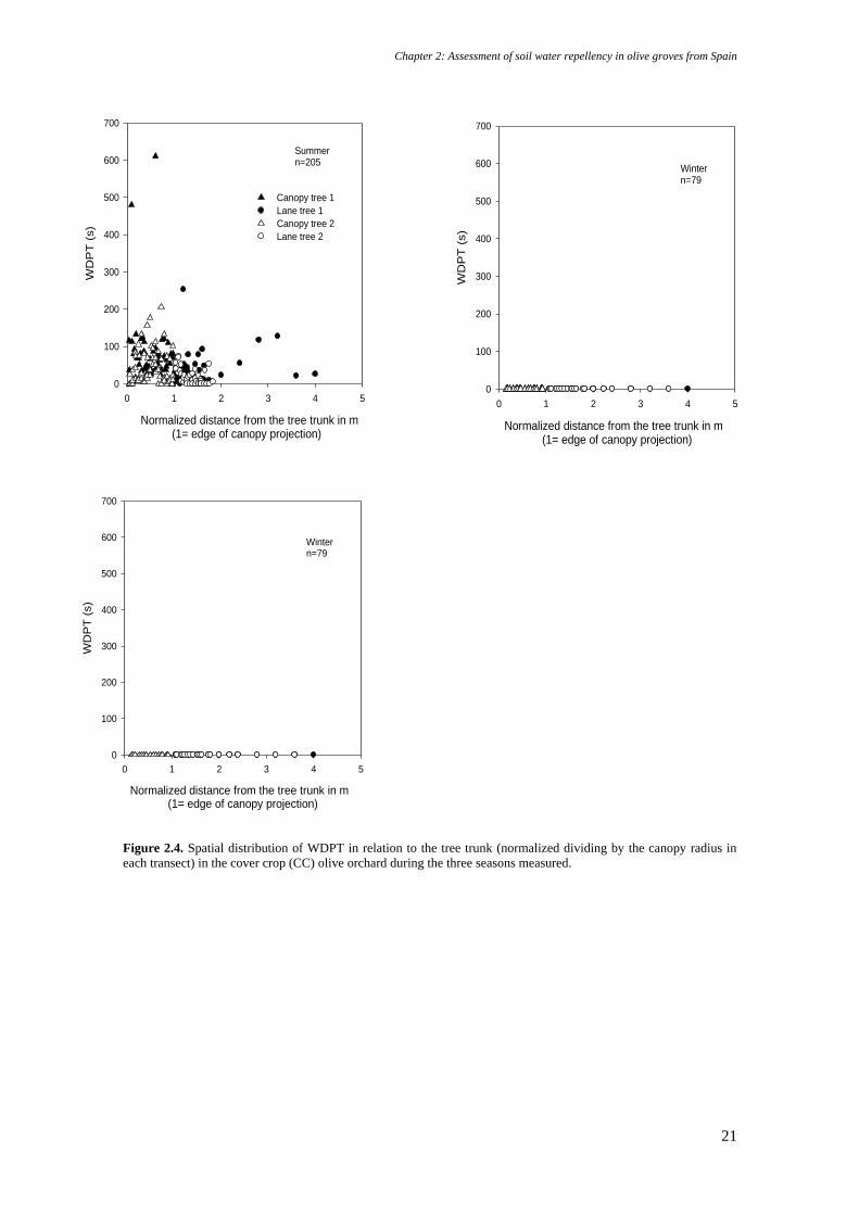
Chapter 2: Assessment of soil water repellency in olive groves from Spain
21
Figure 2.4. Spatial distribution of WDPT in relation to the tree trunk (normalized dividing by the canopy radius in
each transect) in the cover crop (CC) olive orchard during the three seasons measured.
Normalized distance from the tree trunk in m (1= edge of canopy projection)
0 1 2 3 4 5
WD
PT
(s)
0
100
200
300
400
500
600
700
Canopy tree 1
Lane tree 1
Canopy tree 2
Lane tree 2
Summer n=205
Normalized distance from the tree trunk in m (1= edge of canopy projection)
0 1 2 3 4 5
WD
PT
(s)
0
100
200
300
400
500
600
700
Winter n=79
Normalized distance from the tree trunk in m (1= edge of canopy projection)
0 1 2 3 4 5
WD
PT
(s)
0
100
200
300
400
500
600
700
Winter n=79

Distributed processes in the runoff and sediment generation and transport in olive groves at different scales
22
2.4.2. Factors explaining occurrence of SWR
In Table 2.5, the variation of the medians of WDPT (the median values were used when the
distribution of the WDPT values did not fit normality), and the amount of organic matter and
soil moisture in relation to the soil management, the location and the study period are presented.
A high variability of WDPT and OM values was observed with absent repellency in the case of
CT and values close to 600 s for H, whilst OM varied between 2.0 % and 14.3 %; the latter was
an extremely high value compared to what is usually found in olive groves (Gómez and
Giráldez, 2010). No correlation was derived from soil moisture while r-Pearson only was
significant for mean OM values of CC.
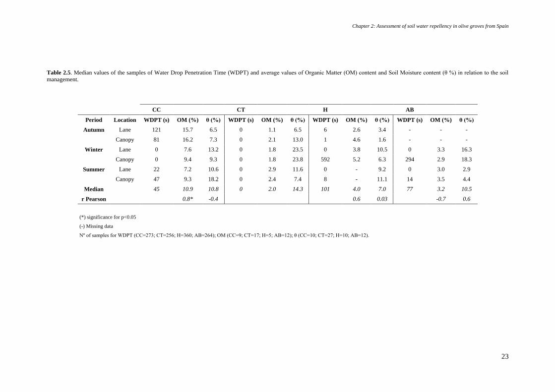
Chapter 2: Assessment of soil water repellency in olive groves from Spain
23
Table 2.5. Median values of the samples of Water Drop Penetration Time (WDPT) and average values of Organic Matter (OM) content and Soil Moisture content (θ %) in relation to the soil
management.
CC CT H AB
Period Location WDPT (s) OM (%) θ (%) WDPT (s) OM (%) θ (%) WDPT (s) OM (%) θ (%) WDPT (s) OM (%) θ (%)
Autumn Lane 121 15.7 6.5 0 1.1 6.5 6 2.6 3.4 - - -
Canopy 81 16.2 7.3 0 2.1 13.0 1 4.6 1.6 - - -
Winter Lane 0 7.6 13.2 0 1.8 23.5 0 3.8 10.5 0 3.3 16.3
Canopy 0 9.4 9.3 0 1.8 23.8 592 5.2 6.3 294 2.9 18.3
Summer Lane 22 7.2 10.6 0 2.9 11.6 0 - 9.2 0 3.0 2.9
Canopy 47 9.3 18.2 0 2.4 7.4 8 - 11.1 14 3.5 4.4
Median 45 10.9 10.8 0 2.0 14.3 101 4.0 7.0 77 3.2 10.5
r Pearson 0.8* -0.4 0.6 0.03 -0.7 0.6
(*) significance for p<0.05
(-) Missing data
Nº of samples for WDPT (CC=273; CT=256; H=360; AB=264); OM (CC=9; CT=17; H=5; AB=12); θ (CC=10; CT=27; H=10; AB=12).
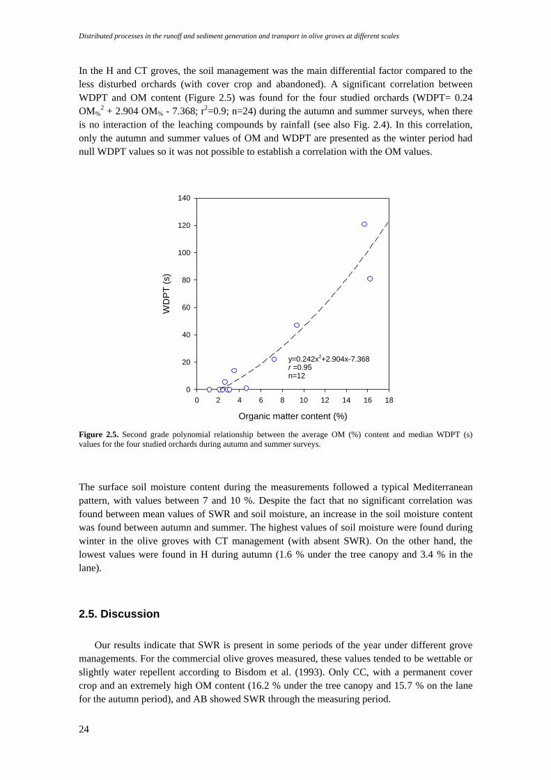
Distributed processes in the runoff and sediment generation and transport in olive groves at different scales
24
In the H and CT groves, the soil management was the main differential factor compared to the
less disturbed orchards (with cover crop and abandoned). A significant correlation between
WDPT and OM content (Figure 2.5) was found for the four studied orchards (WDPT= 0.24
OM%2 + 2.904 OM% - 7.368; r2=0.9; n=24) during the autumn and summer surveys, when there
is no interaction of the leaching compounds by rainfall (see also Fig. 2.4). In this correlation,
only the autumn and summer values of OM and WDPT are presented as the winter period had
null WDPT values so it was not possible to establish a correlation with the OM values.
Figure 2.5. Second grade polynomial relationship between the average OM (%) content and median WDPT (s)
values for the four studied orchards during autumn and summer surveys.
The surface soil moisture content during the measurements followed a typical Mediterranean
pattern, with values between 7 and 10 %. Despite the fact that no significant correlation was
found between mean values of SWR and soil moisture, an increase in the soil moisture content
was found between autumn and summer. The highest values of soil moisture were found during
winter in the olive groves with CT management (with absent SWR). On the other hand, the
lowest values were found in H during autumn (1.6 % under the tree canopy and 3.4 % in the
lane).
2.5. Discussion
Our results indicate that SWR is present in some periods of the year under different grove
managements. For the commercial olive groves measured, these values tended to be wettable or
slightly water repellent according to Bisdom et al. (1993). Only CC, with a permanent cover
crop and an extremely high OM content (16.2 % under the tree canopy and 15.7 % on the lane
for the autumn period), and AB showed SWR through the measuring period.
Organic matter content (%)
0 2 4 6 8 10 12 14 16 18
WD
PT
(s)
0
20
40
60
80
100
120
140
y=0.242x2+2.904x-7.368
r =0.95n=12
Chapter 2: Assessment of soil water repellency in olive groves from Spain
25
The different soil managements in the groves, rainfall data observed in each location, slope and
soil type and characteristics, suggest that the appearance and magnitude of SWR in this system
will be moderate, developing during the dry season and being reduced (or disappearing) during
the rainfall season as the organic compounds reoriented and turn amphiphilic.
Both CC and AB had hydrophobic spots under the tree canopy. The highest values of WDPT
and OM were found under the tree canopy which agrees with authors such as Scholl (1971) who
showed that SWR was confined to the soil under the tree canopy. In AB, it is apparent that the
soil moisture content might control the appearance of repellency in summer. In addition, the soil
under tree canopies is usually unaltered or less altered, which improves soil characteristics such
as soil organic C accumulation, water retention, water infiltration, hydraulic conductivity,
microbial activity and other soil processes in olives (e.g. Gómez et al. 1999) or field crops (e.g.
Blanco-Canqui and Lal. 2009). Hence, if the soil structure is stable, the soil porosity enhances
and the probability of runoff and erosion processes decrease (Bronick and Lal, 2005).
CT and H showed wettable ('subcritical') values of SWR. Repellency in CT might be controlled
by its soil texture as the percentage of clays is high (note that clays such as kaolinite have been
used to reduce soil water repellency of sandy soils, Ma'shum et al., 1989; Cann and Lewis,
1994; McKissock et al., 2000). In this orchard, the OM is also low compared to the others used
in our study but within the values found in most olive groves from Spain, which means that the
hydrophobic inputs are not as high as in the rest and the mineralization rates are higher
(González-Peñaloza et al., 2012). Therefore, strong water repellent values are not expected,
particularly because the soil expands when it gets wet. Moreover, tillage operations must also
contribute to reduce SWR in the top soil as Urbanek et al. (2007) reported. For H, where
management operations are less intense, organic matter mineralization rates can result higher,
reducing SWR.
On the other hand, the exponential correlation between organic matter and the SWR during the
dry periods of the year (summer and autumn) suggests that the organic matter of the top 5-cm of
the soil might be used as a proxy variable to identify preliminarily orchards prone to SWR
under Mediterranean environments, particularly in areas with high soil vegetation cover (such as
CC and AB). Soil organic matter in olive crops has hydrophobic compounds such as
Polyphenols, Sterols, Nonsterol, Triterpenoids or Pentacyclic triterpenoids (Briante et al., 2002;
Stiti and Hartmann, 2012; Peragón, 2013), which decompose in the soil coating soil aggregates.
These differences can be explained by the amount of rainfall in the AB site between the winter
sampling period (28/12/2011) and the summer sampling period (29/7/2012) equal to 29.7 mm
(SIAR, 2013), whereas in CC and H was 146.1 mm, between the 19/12/2011 and the
20/07/2012 (IFAPA, Estación de Alameda del Obispo, 2013).
Beyond the exponential correlation between soil organic matter and WDPT during the autumn
and summer seasons, we did not find that the organic matter and gravimetric soil moisture in the
different olive groves were significantly correlated. In our results, it is apparent that the negative
effect of the rainfall season on soil water repellency is the major source of variability given the
limited disturbance of the soil in the studied orchards.
The magnitude of the SWR measurements was not significantly larger than those measured by
other authors in olive groves in similar environments, in commercial (Ziogas et al., 2005) or
wild (Zavala et al., 2009) olive groves. Even though, under the tree canopy, the WDPT values
were strongly water repellent, its influence in the runoff response of the grove may be small due
Distributed processes in the runoff and sediment generation and transport in olive groves at different scales
26
to the high spatial variability with nearby areas with non-hydrophobic values which might act as
run-on areas, something observed in olive groves (Castro et al., 2006).
A major feature in understanding the hydrological role of hydrophobicity in olive groves was
the large spatial variability found in our measurements. A source of spatial variability was the
location with relation to the olive tree crown canopy. The area underneath the tree canopy was
the main influence site, although not in a permanent way, apart from in the AB grove; where
notable differences were observed in soil water repellency between canopy and row. The size of
the canopy, variable among orchards, might implicate bigger/smaller influence radius of SWR
as this would increase or decrease the availability of hydrophobic compounds.
High spatial variability at short distances was also found in our measurements. This showed
SWR patchiness in most of the studied groves, indicating the coexistence of points with
relatively high SWR values and others with low or non-existing SWR. This 'patchiness',
combined with the low persistence of repellency when wet might explain why the under canopy
areas is, simultaneously, an area slightly hydrophobic and an area with a high infiltration rate
when measured using different techniques and teams on many groves (e.g. Romero et al., 2007).
Our hypothesis is that this patchiness results in a high probability that the rainfall drop will
eventually infiltrate in a nearby non-hydrophobic area with a larger infiltration capacity during
the short period (some minutes) when repellency is still present. These phenomena have been
observed and modelled at a slightly larger scale in the interaction between the lane and the
below canopy area using numerical models and experimentally demonstrated using large-scale
rainfall simulation (Castro et al., 2006). Additionally, the below canopy area is subjected to less
rainfall (especially during the early stages of a rainfall event) due to rainfall interception by the
olive canopy (Gómez et al., 2001, 2002). This extends the time period for soil wetting at a low
rainfall intensity, which could mean the reduction of SWR during the early stages of a rainfall
event.
Further studies taking into account spatial variability in the field and its correlation with soil
properties, such as microrelief and orientation, and above ground vegetation at microscale;
could provide additional insight into the correlation of SWR and other soil properties, as well as
its environmental implications in olive groves. For instance to explain the differences of
infiltration and runoff between lane and canopy areas and the large spatial variability in
infiltration measured in olive groves (Gómez et al., 1999).
2.6. Conclusions
The temporal and spatial approach carried out has demonstrated that SWR can occur in
olive groves although a high variability was observed. No permanent spatial pattern lane/canopy
was found. However, the highest values were mostly found under the canopy, whose the most
evident influence was in the organic olive grove. The combination of soil moisture and organic
matter could not globally explain the differences of soil water repellency in the olive groves;
although a clear correlation among organic matter content and soil water repellency was found
for the summer and autumn season in the four olive groves. Our measurements also indicate a
patchiness of soil water repellency in the olive groves. These results suggest that the
hydrological relevance of soil water repellency in olive groves could be low for spatial scales
beyond point measurements, such as hillslope or catchment. However, it can contribute to
explain the differences of infiltration and runoff between lane and canopy areas.

Chapter 2: Assessment of soil water repellency in olive groves from Spain
27
Acknowledgements
The authors would like to thank José Antonio Burguet for his full help and support during
the fieldwork. This study was supported by the Project P08-AGR-03925 (Andalusian
Government), AGL2009-12936-C03-01 (Ministry of Science and Innovation), RESEL
(Ministry of Agriculture, Food and Environment) and FEDER fund. The program JAE of the
National Spanish Research Centre, which provided grant support for the PhD project of the
corresponding author, is also thanked.

Distributed processes in the runoff and sediment generation and transport in olive groves at different scales
28
Chapter 3: Evaluating grass strips trapping efficiency using a magnetic iron oxide as a tracer
29
Chapter 3
Evaluating grass strips trapping
efficiency using magnetic iron oxide as a tracer
Part of the results of this chapter has been presented as a communication in:
European Geoscience Union, EGU (2013):
Burguet, M., Guzmán, G., Taguas, E.V., Gómez, J. A.: Evaluating grass strips trapping
efficiency using magnetic iron as a tracer. European Geoscience Union, EGU, 2013
Young Scientist's Travel Award, EGU, 2013
‘The conservation of natural resources is the fundamental problem. Unless we solve that
problem, it will avail us little to solve all others’.
Theodore Roosevelt (1858-1919)

Distributed processes in the runoff and sediment generation and transport in olive groves at different scales
30
Chapter 3: Evaluating grass strips trapping efficiency using a magnetic iron oxide as a tracer
31
Resumen
El uso de cubiertas vegetales ha sido prescrito como medida de mitigación de la erosión
dado que las cubiertas permanentes han demostrado ser efectivas tanto en la reducción de
sedimentos como en las descargas de agroquímicos. Los objetivos principales de este trabajo
fueron: [1] explorar el uso combinado de la lluvia natural y la lluvia simulada con óxido
magnético con el fin de entender el comportamiento de las bandas de cubierta en la retención de
la escorrentía y las pérdidas de suelo a escala de parcela y, [2] evaluar el grado de efectividad de
las bandas de cubierta a la hora de tamponar el sedimento procedente de las áreas con suelo
desnudo bajo diferentes condiciones comparado con una situación control sin bandas. Este
estudio abarca seis simulaciones de lluvia bajo cuatro manejos de suelo diferentes en las que se
combina el uso de óxido magnético como trazador de sedimento con el fin de obtener una mejor
comprensión de la eficiencia de atrape de las bandas de cubierta. Con este fin se instalaron tres
parcelas de escorrentía de 6 m x 14 m en una ladera de terraza aluvial (Fluvisol) con una
pendiente de 20 %. Cada una de las parcelas contiene tres bandas de suelo desnudo marcado con
óxido magnético y tres bandas con cubierta de Lolium multiflorum L. Los manejos de suelo
simulados fueron: inmediatamente después de plantar las cubiertas vegetales (Junio 2011cubierta
vegetal), con cubierta vegetal agostada (Junio 2012cubierta vegetal), después de labrar a una
profundidad de 5 cm (Octubre 2013recién arado) y después de labrar y compactar mecánicamente el
suelo con una plancha de metal (Noviembre 2013superficie consolidada). Nuestros resultados indican
que, mediante el uso de bandas de cubierta, la escorrentía y la pérdida de sedimento fueron
aproximadamente el 50 % y el 12 % respectivamente más bajos que los valores medidos en
suelo desnudo consolidado o recién labrado. La formación de microrelieve en las parcelas en
forma de escalones después de la primera simulación ayudó asimismo a la reducción de las
pérdidas de suelo y escorrentía. El manejo de suelo correspondiente al laboreo y posterior
compactación obtuvieron las tasas más elevadas de escorrentía acumulada y pérdidas de suelo
(28 mm y 15 kg respectivamente). Se observó una evidente selectividad en el transporte del
trazador propiciado por las partículas de suelo de texturas más finas (arcillas) dado que el
sedimento recogido en las simulaciones estaba enriquecido de éstas. Estas características
contribuyen a explicar los efectos del manejo y de la vegetación en las distribución de
sedimentos en laderas y deben ser tenidas en cuenta a la hora de llevar a cabo estudios con
trazadores así como con bandas de cubiertas para mitigar la contaminación por agroquímicos.
Palabras clave: bandas de cubierta, trazador magnético, manejo de suelo, selectividad en el
transporte, lluvia simulada.
Distributed processes in the runoff and sediment generation and transport in olive groves at different scales
32
Abstract
The use of cover crops has been prescribed as a mitigation measure for both problems
because permanent cover crops have demonstrated to reduce sediment and agrochemical loads.
The objectives of the present study were twofold: [1] to explore the combined use of natural and
simulated rainfall and magnetic iron oxide in understanding the performance of vegetation strips
on runoff and soil losses at plot scale and, [2] to evaluate the effectiveness degree of vegetation
strips in buffering sediment from bare soil areas under different conditions compared to a
control situation with no strips. This study encompasses six rainfall simulations under four
different soil managements combining the use of a magnetic iron oxide as a sediment tracer to
obtain a better understanding of the vegetation strips trapping efficiency. Three runoff plots of 6
m × 14 m were established in a 20% hillslope under a Fluvisol alluvial terrace. Each of the plots
contained three bare strips tagged with magnetic iron oxide and three strips with Lolium
multiflorum L. The soil management simulated scenarios were: immediately after sowing the
vegetation cover (June 2011cover crop), with settled vegetation cover (June 2012cover crop), after 5
cm of deep ploughing (October 2013freshly tilled) and after ploughing and mechanically compacting
the soil with a sheet metal (November 2013 consolidated surface). Our results indicate that by using
cover crop strips, runoff and sediment losses were approximately 50 % and 12 % respectively
lower than the measured values in bare consolidated and freshly tilled soil. The formation of
microrelief steps after the first simulation also helped to reduce soil losses and runoff. Ploughed
and compacted soil management showed the highest cumulative runoff and soil losses values
(28 mm and 15 kg). Evident tracer selectivity from small particle size soil textures (clays) was
observed as there was an enrichment of these particles in the collected sediment. These features
contribute to explain the effects of the management and the vegetation on the sediment
distribution in the hillslopes and must be taken into account when performing tracing studies as
well as when using cover crop strips to mitigate offsite contamination by agrochemicals.
Keywords: vegetation strips, magnetic tracer, soil management, selective transport, rainfall
simulations.
Chapter 3: Evaluating grass strips trapping efficiency using a magnetic iron oxide as a tracer
33
3.1. Introduction
Water erosion and associated offsite contamination are major environmental risks in
many Mediterranean crops such as olives or vineyards (Beaufoy, 2001; Gómez et al., 2011).
The use of cover crops has been prescribed as a mitigation measure for both problems because
permanent cover crops have demonstrated to reduce sediment and agrochemical loads (e.g.
Gómez, 2009a; 2009b). However, large uncertainty remains about its effectiveness degree to
reduce sediment and agrochemical contribution to streams due to the limited number of
available studies, and the large variability observed under field conditions (Taguas et al., 2012).
Grass strips are described as permanent vegetation or part of the crop rotation cycle which are
set out along contour lines, separated by strips of arable land (van Dijk et al., 1996). They work
hydraulically increasing roughness to reduce flow velocity and promoting sediment deposition
as well as adsorption by the vegetation. Its impact on erosion has been modelled for empirical,
e.g. RUSLE (Renard et al., 1997) and physically based models, e.g. TRAVA (Deletic and
Fletcher, 2006). The combination of experimental and modelling analyses indicate that a broad
range of efficiency degrees of grass strips in sediment trapping and in filtering are expected. For
instance, Al-wadaey et al. (2012) found a reduction of 50 % in sediment and phosphorus
contribution using filter strips of tall fescue and orchard grasses which covered, in average, a 3
% of the plot area. Kapil et al. (2010) in a review of efficiency of filter strips on sediment and
pesticide offsite contamination found an average reduction of 45 % in runoff volume (ranging
between 0 and 100 %) and an average of 76 % in sediment mass (ranging between 2 and 100
%). This variability reflected, among other issues, that there were several factors such as slope,
type of vegetation and its degree of development (Xiao et al., 2011; Thayer et al., 2012) which
affect significantly the efficiency of filter strips. In addition, the development of microrelief in
the strip boundary leaded to the development of rill erosion that could breach the strips and
decrease their efficiency (Pankau et al., 2012).
A better understanding of the mechanisms controlling the hydraulics and sediment retention
capacity of vegetation strips can be obtained from the calibration of models to extrapolate the
available experimental data to the wide variety of scenarios (Fox et al., 2013) which eventually
allow improving the effectiveness of their use in farm conditions. Furthermore, the
determination of sediment sources using suitable sediment tracing/fingerprinting properties has
been noted as one tool to evaluate the effectiveness and functioning of vegetated filters at the
catchment scale (Koiter et al., 2013). At the small hillslope scale, the use of sediment tracers can
provide insight about the origin and path of sediment trapped by vegetation strips. Guzmán et al.
(2010a) developed a tracing technique based on magnetic iron oxides successfully used to
determine differences in erosion rates within an olive orchard at plot scale (Guzmán et al.,
2013). This tracer can be potentially used for evaluating the trapping efficiency of vegetation
strips in conditions similar to those found in orchards under Mediterranean conditions.
The objectives of the present study are twofold: [1] to explore the combined use of natural and
simulated rainfall and magnetic iron oxide in understanding the performance of vegetation strips
on runoff and soil losses at plot scale and, [2] to evaluate the effectiveness degree of vegetation
strips in buffering sediment from bare soil areas under different conditions compared to a
control situation with no strips.
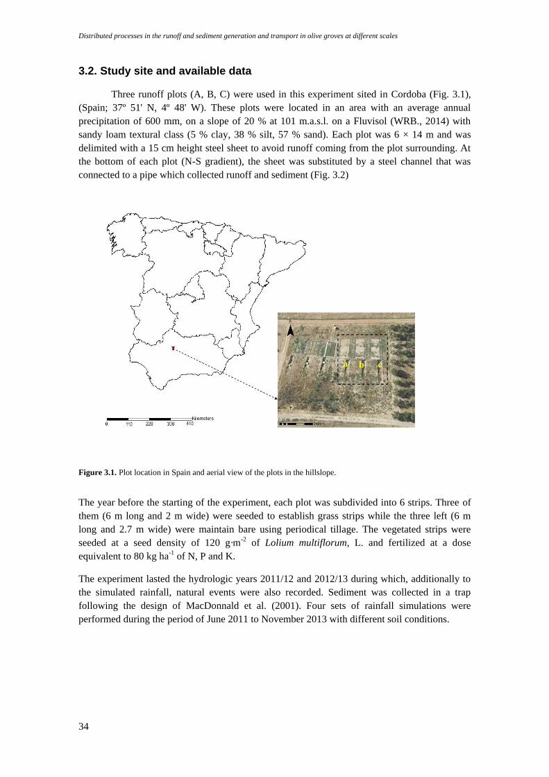
Distributed processes in the runoff and sediment generation and transport in olive groves at different scales
34
3.2. Study site and available data
Three runoff plots (A, B, C) were used in this experiment sited in Cordoba (Fig. 3.1),
(Spain; 37º 51' N, 4º 48' W). These plots were located in an area with an average annual
precipitation of 600 mm, on a slope of 20 % at 101 m.a.s.l. on a Fluvisol (WRB., 2014) with
sandy loam textural class (5 % clay, 38 % silt, 57 % sand). Each plot was 6 × 14 m and was
delimited with a 15 cm height steel sheet to avoid runoff coming from the plot surrounding. At
the bottom of each plot (N-S gradient), the sheet was substituted by a steel channel that was
connected to a pipe which collected runoff and sediment (Fig. 3.2)
Figure 3.1. Plot location in Spain and aerial view of the plots in the hillslope.
The year before the starting of the experiment, each plot was subdivided into 6 strips. Three of
them (6 m long and 2 m wide) were seeded to establish grass strips while the three left (6 m
long and 2.7 m wide) were maintain bare using periodical tillage. The vegetated strips were
seeded at a seed density of 120 g·m-2 of Lolium multiflorum, L. and fertilized at a dose
equivalent to 80 kg ha-1 of N, P and K.
The experiment lasted the hydrologic years 2011/12 and 2012/13 during which, additionally to
the simulated rainfall, natural events were also recorded. Sediment was collected in a trap
following the design of MacDonnald et al. (2001). Four sets of rainfall simulations were
performed during the period of June 2011 to November 2013 with different soil conditions.
a b c
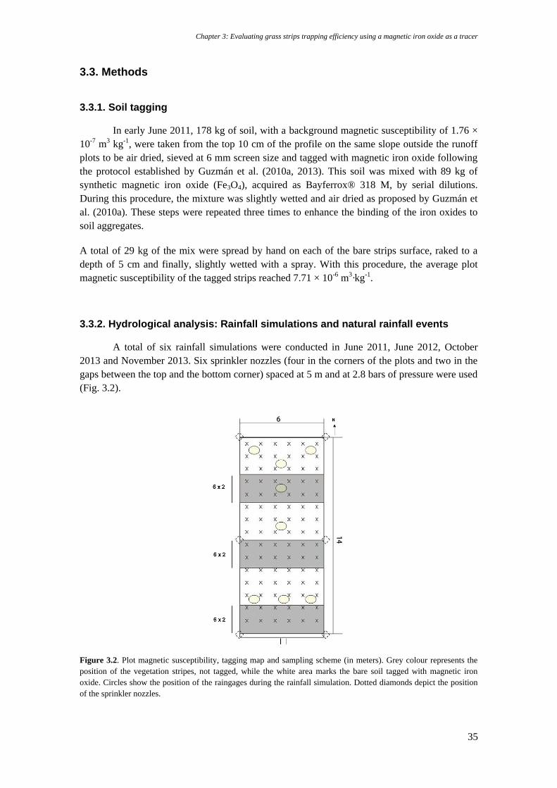
Chapter 3: Evaluating grass strips trapping efficiency using a magnetic iron oxide as a tracer
35
3.3. Methods
3.3.1. Soil tagging
In early June 2011, 178 kg of soil, with a background magnetic susceptibility of 1.76 ×
10-7 m3 kg-1, were taken from the top 10 cm of the profile on the same slope outside the runoff
plots to be air dried, sieved at 6 mm screen size and tagged with magnetic iron oxide following
the protocol established by Guzmán et al. (2010a, 2013). This soil was mixed with 89 kg of
synthetic magnetic iron oxide (Fe3O4), acquired as Bayferrox® 318 M, by serial dilutions.
During this procedure, the mixture was slightly wetted and air dried as proposed by Guzmán et
al. (2010a). These steps were repeated three times to enhance the binding of the iron oxides to
soil aggregates.
A total of 29 kg of the mix were spread by hand on each of the bare strips surface, raked to a
depth of 5 cm and finally, slightly wetted with a spray. With this procedure, the average plot
magnetic susceptibility of the tagged strips reached 7.71 × 10⁻⁶ m3·kg-1.
3.3.2. Hydrological analysis: Rainfall simulations and natural rainfall events
A total of six rainfall simulations were conducted in June 2011, June 2012, October
2013 and November 2013. Six sprinkler nozzles (four in the corners of the plots and two in the
gaps between the top and the bottom corner) spaced at 5 m and at 2.8 bars of pressure were used
(Fig. 3.2).
Figure 3.2. Plot magnetic susceptibility, tagging map and sampling scheme (in meters). Grey colour represents the
position of the vegetation stripes, not tagged, while the white area marks the bare soil tagged with magnetic iron
oxide. Circles show the position of the raingages during the rainfall simulation. Dotted diamonds depict the position
of the sprinkler nozzles.
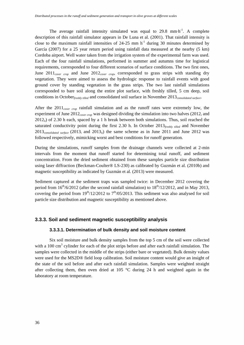
Distributed processes in the runoff and sediment generation and transport in olive groves at different scales
36
The average rainfall intensity simulated was equal to 29.8 mm·h-1. A complete
description of this rainfall simulator appears in De Luna et al. (2001). That rainfall intensity is
close to the maximum rainfall intensities of 24-25 mm h-1 during 30 minutes determined by
García (2007) for a 25 year return period using rainfall data measured at the nearby (5 km)
Cordoba airport. Well water taken from the irrigation system of the experimental farm was used.
Each of the four rainfall simulations, performed in summer and autumns time for logistical
requirements, corresponded to four different scenarios of surface conditions. The two first ones,
June 2011cover crop and June 2012cover crop, corresponded to grass strips with standing dry
vegetation. They were aimed to assess the hydrologic response to rainfall events with good
ground cover by standing vegetation in the grass strips. The two last rainfall simulations
corresponded to bare soil along the entire plot surface, with freshly tilled, 5 cm deep, soil
conditions in Octoberfreshly tilled and consolidated soil surface in November 2013consolidated surface.
After the 2011cover crop rainfall simulation and as the runoff rates were extremely low, the
experiment of June 2012cover crop was designed dividing the simulation into two halves (2012i and
2012ii) of 2.30 h each, spaced by a 1 h break between both simulations. Thus, soil reached the
saturated conductivity point during the first 2.30 h. In October 2013freshly tilled and November
2013consolidated surface (2013i and 2013ii) the same scheme as in June 2011 and June 2012 was
followed respectively, mimicking worst and best conditions for runoff generation.
During the simulations, runoff samples from the drainage channels were collected at 2-min
intervals from the moment that runoff started for determining total runoff, and sediment
concentration. From the dried sediment obtained from these samples particle size distribution
using laser diffraction (Beckman-Coulter® LS-230) as calibrated by Guzmán et al. (2010b) and
magnetic susceptibility as indicated by Guzmán et al. (2013) were measured.
Sediment captured at the sediment traps was sampled twice: in December 2012 covering the
period from 16th/6/2012 (after the second rainfall simulation) to 18th/12/2012, and in May 2013,
covering the period from 19th/12/2012 to 7th/05/2013. This sediment was also analysed for soil
particle size distribution and magnetic susceptibility as mentioned above.
3.3.3. Soil and sediment magnetic susceptibility analysis
3.3.3.1. Determination of bulk density and soil moisture content
Six soil moisture and bulk density samples from the top 5 cm of the soil were collected
with a 100 cm3 cylinder for each of the plot strips before and after each rainfall simulation. The
samples were collected in the middle of the strips (either bare or vegetated). Bulk density values
were used for the MS2D® field loop calibration. Soil moisture content would give an insight of
the state of the soil before and after each rainfall simulation. Samples were weighted straight
after collecting them, then oven dried at 105 °C during 24 h and weighted again in the
laboratory at room temperature.
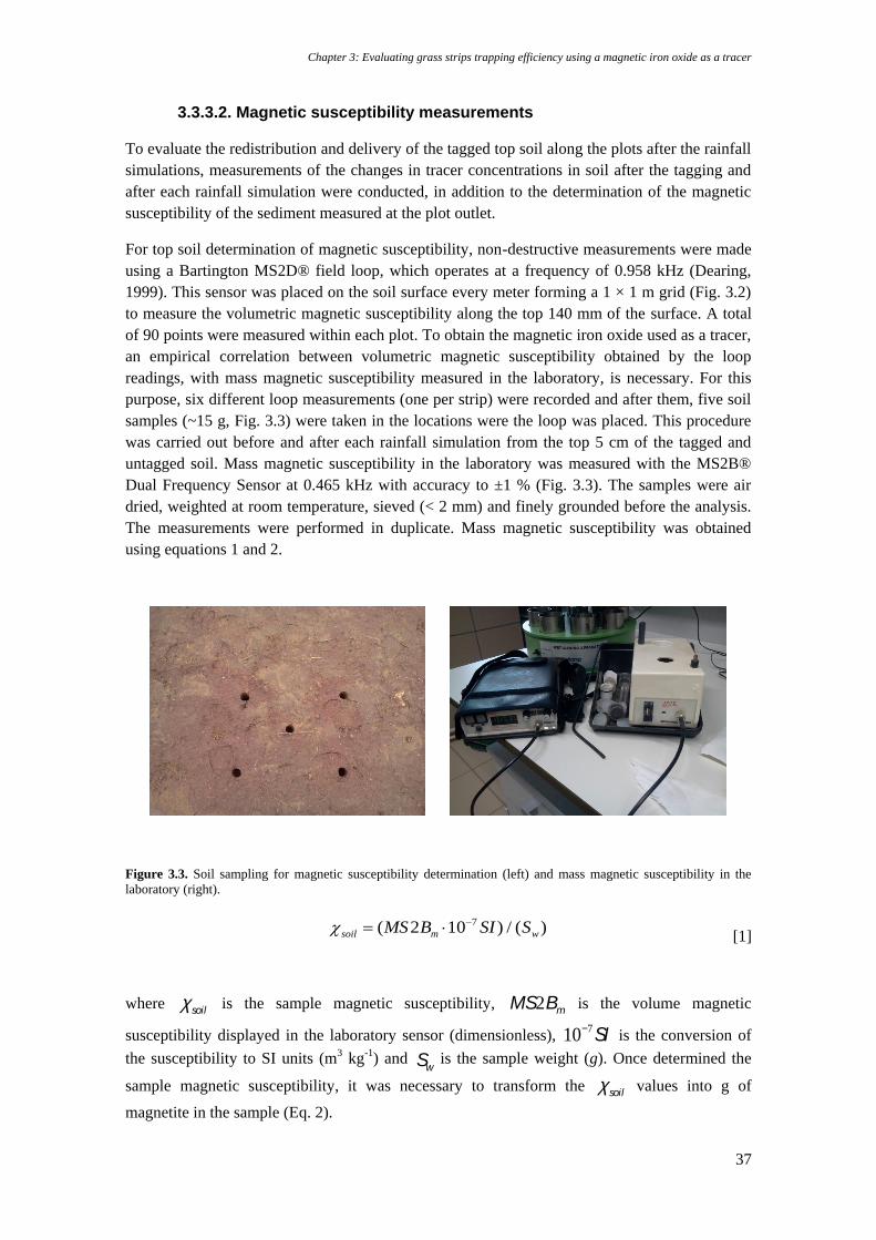
Chapter 3: Evaluating grass strips trapping efficiency using a magnetic iron oxide as a tracer
37
3.3.3.2. Magnetic susceptibility measurements
To evaluate the redistribution and delivery of the tagged top soil along the plots after the rainfall
simulations, measurements of the changes in tracer concentrations in soil after the tagging and
after each rainfall simulation were conducted, in addition to the determination of the magnetic
susceptibility of the sediment measured at the plot outlet.
For top soil determination of magnetic susceptibility, non-destructive measurements were made
using a Bartington MS2D® field loop, which operates at a frequency of 0.958 kHz (Dearing,
1999). This sensor was placed on the soil surface every meter forming a 1 × 1 m grid (Fig. 3.2)
to measure the volumetric magnetic susceptibility along the top 140 mm of the surface. A total
of 90 points were measured within each plot. To obtain the magnetic iron oxide used as a tracer,
an empirical correlation between volumetric magnetic susceptibility obtained by the loop
readings, with mass magnetic susceptibility measured in the laboratory, is necessary. For this
purpose, six different loop measurements (one per strip) were recorded and after them, five soil
samples (~15 g, Fig. 3.3) were taken in the locations were the loop was placed. This procedure
was carried out before and after each rainfall simulation from the top 5 cm of the tagged and
untagged soil. Mass magnetic susceptibility in the laboratory was measured with the MS2B®
Dual Frequency Sensor at 0.465 kHz with accuracy to ±1 % (Fig. 3.3). The samples were air
dried, weighted at room temperature, sieved (< 2 mm) and finely grounded before the analysis.
The measurements were performed in duplicate. Mass magnetic susceptibility was obtained
using equations 1 and 2.
Figure 3.3. Soil sampling for magnetic susceptibility determination (left) and mass magnetic susceptibility in the
laboratory (right).
7( 2 10 ) / ( )soil m wMS B SI S
[1]
where csoil is the sample magnetic susceptibility, MS2Bm
is the volume magnetic
susceptibility displayed in the laboratory sensor (dimensionless), 10-7SI is the conversion of
the susceptibility to SI units (m3 kg-1) and Sw is the sample weight (g). Once determined the
sample magnetic susceptibility, it was necessary to transform the csoil values into g of
magnetite in the sample (Eq. 2).

Distributed processes in the runoff and sediment generation and transport in olive groves at different scales
38
[2]
where gtare the g of tracer in the sample, m is the theoretical mass of tracer that would fit in
the soil sampler and is in function of the sample bulk density in g cm-3, csoil is the sample
magnetic susceptibility determined as in Eq. 1, cbackground is the soil background magnetic
susceptibility and cFe3O4is the magnetic iron oxide susceptibility.
The empirical relationship between the volume susceptibilities and the grams of tracer obtained
is shown in Fig. 3.4. This relation was used to convert the loop values into magnetite content for
mapping tracer redistribution within the plots after the rainfall simulations.
Figure 3.4. MS2D field loop and MS2B laboratory sensor calibration for mapping magnetic susceptibility along the
plots.
3.3.3.3. Modeling spatial sediment patterns: mixing model
A mixing model (Eq. 3) developed by Guzmán et al. (2013) was used to determine the
sources of the sediment after rainfall events. In this case the sources are on one hand, the
vegetation strips (untagged soil) and, on the other hand, the bare soil (tagged). An α coefficient
(Eq. 4) which encompasses the selectivity and distribution processes of the tracer was included
in the calculation.
(1 )sed b b v bf f [3]
s dc c [4]
MS2D loop measurements
0 200 400 600 800 1000 1200 1400 1600
MS
2B
ma
gn
etite
co
nte
nt (g
)
0.00
0.20
0.40
0.60
0.80
1.00
y= 0.0006x+0.0078r = 0.95n = 62
3 4Fe O( ) / ( )t soil background backgroundg m
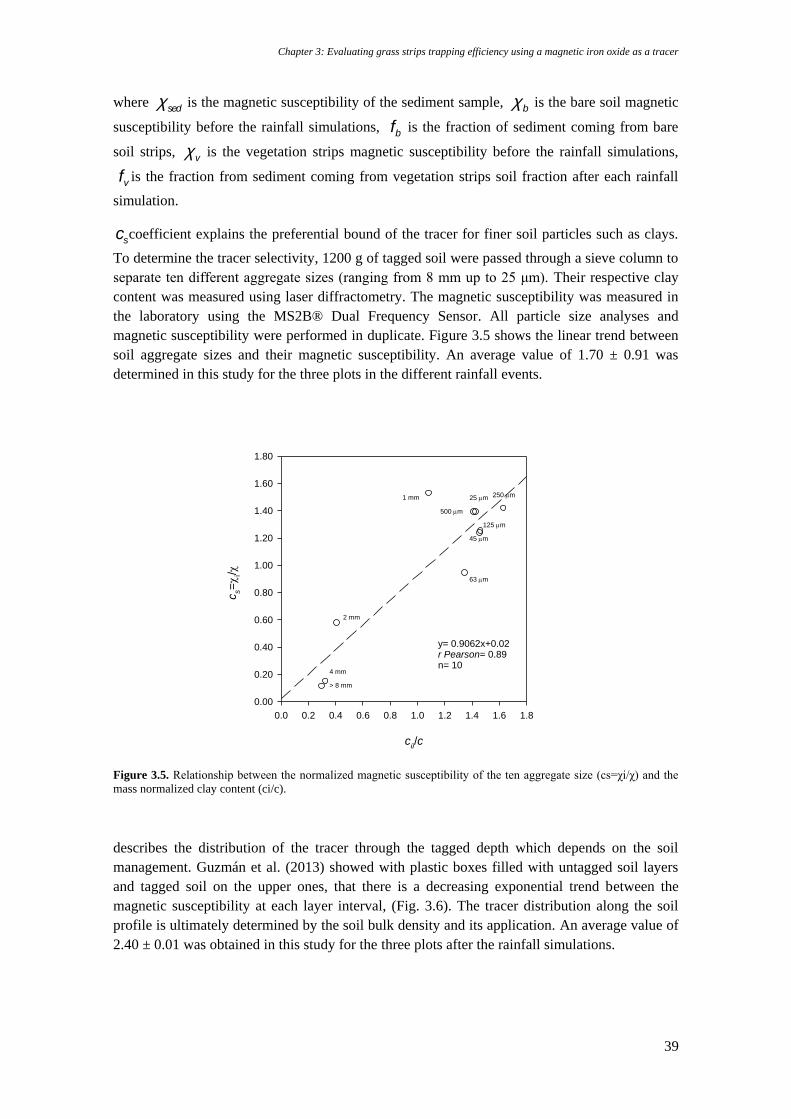
Chapter 3: Evaluating grass strips trapping efficiency using a magnetic iron oxide as a tracer
39
where csed is the magnetic susceptibility of the sediment sample, cb
is the bare soil magnetic
susceptibility before the rainfall simulations, fb is the fraction of sediment coming from bare
soil strips, c v is the vegetation strips magnetic susceptibility before the rainfall simulations,
fvis the fraction from sediment coming from vegetation strips soil fraction after each rainfall
simulation.
cscoefficient explains the preferential bound of the tracer for finer soil particles such as clays.
To determine the tracer selectivity, 1200 g of tagged soil were passed through a sieve column to
separate ten different aggregate sizes (ranging from 8 mm up to 25 μm). Their respective clay
content was measured using laser diffractometry. The magnetic susceptibility was measured in
the laboratory using the MS2B® Dual Frequency Sensor. All particle size analyses and
magnetic susceptibility were performed in duplicate. Figure 3.5 shows the linear trend between
soil aggregate sizes and their magnetic susceptibility. An average value of 1.70 ± 0.91 was
determined in this study for the three plots in the different rainfall events.
Figure 3.5. Relationship between the normalized magnetic susceptibility of the ten aggregate size (cs=χi/χ) and the
mass normalized clay content (ci/c).
describes the distribution of the tracer through the tagged depth which depends on the soil
management. Guzmán et al. (2013) showed with plastic boxes filled with untagged soil layers
and tagged soil on the upper ones, that there is a decreasing exponential trend between the
magnetic susceptibility at each layer interval, (Fig. 3.6). The tracer distribution along the soil
profile is ultimately determined by the soil bulk density and its application. An average value of
2.40 ± 0.01 was obtained in this study for the three plots after the rainfall simulations.
0.0 0.2 0.4 0.6 0.8 1.0 1.2 1.4 1.6 1.8
0.00
0.20
0.40
0.60
0.80
1.00
1.20
1.40
1.60
1.80
cii/c
cs=
i/
y= 0.9062x+0.02r Pearson= 0.89n= 10
> 8 mm
4 mm
2 mm
63 m
1 mm 250 m
45 m
125 m
500 m
25 m
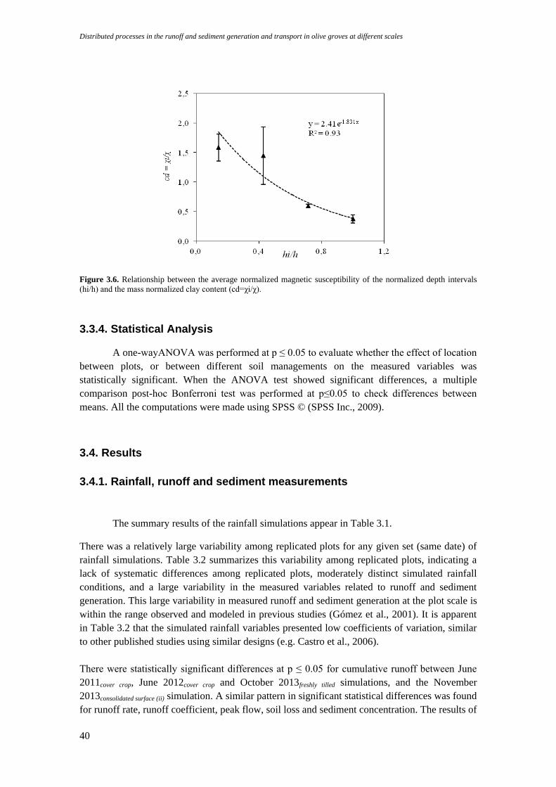
Distributed processes in the runoff and sediment generation and transport in olive groves at different scales
40
Figure 3.6. Relationship between the average normalized magnetic susceptibility of the normalized depth intervals
(hi/h) and the mass normalized clay content (cd=χi/χ).
3.3.4. Statistical Analysis
A one-wayANOVA was performed at p ≤ 0.05 to evaluate whether the effect of location
between plots, or between different soil managements on the measured variables was
statistically significant. When the ANOVA test showed significant differences, a multiple
comparison post-hoc Bonferroni test was performed at p≤0.05 to check differences between
means. All the computations were made using SPSS © (SPSS Inc., 2009).
3.4. Results
3.4.1. Rainfall, runoff and sediment measurements
The summary results of the rainfall simulations appear in Table 3.1.
There was a relatively large variability among replicated plots for any given set (same date) of
rainfall simulations. Table 3.2 summarizes this variability among replicated plots, indicating a
lack of systematic differences among replicated plots, moderately distinct simulated rainfall
conditions, and a large variability in the measured variables related to runoff and sediment
generation. This large variability in measured runoff and sediment generation at the plot scale is
within the range observed and modeled in previous studies (Gómez et al., 2001). It is apparent
in Table 3.2 that the simulated rainfall variables presented low coefficients of variation, similar
to other published studies using similar designs (e.g. Castro et al., 2006).
There were statistically significant differences at p ≤ 0.05 for cumulative runoff between June
2011cover crop, June 2012cover crop and October 2013freshly tilled simulations, and the November
2013consolidated surface (ii) simulation. A similar pattern in significant statistical differences was found
for runoff rate, runoff coefficient, peak flow, soil loss and sediment concentration. The results of

Chapter 3: Evaluating grass strips trapping efficiency using a magnetic iron oxide as a tracer
41
the rainfall simulations are splitted into two sets that can be associated with different surface
conditions. Although surface conditions were markedly different between some dates, the initial
soil moisture of the top soil in the beginning of the four blocks of rainfall simulations (June
2011cover crop, June 2012cover crop (i), October 2013freshly tilled and November 2013consolidated surface (i) was
similar, with an average volumetric soil water content in the top 5 cm of the soil of 10.9 %
without statistically significant differences between plots and different dates. Obviously the
initial soil moisture in the two rainfall simulations preformed after a 1 h break (June 2012cover crop
(ii) and November 2013consolidated surface (ii)) was much greater, with an average value of 20.1%. Soil
conditions varied markedly between different rainfall simulation blocks.
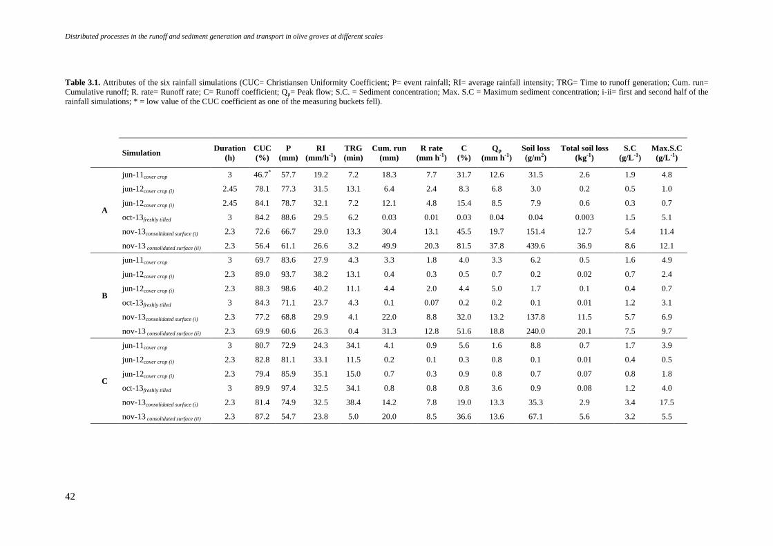
Distributed processes in the runoff and sediment generation and transport in olive groves at different scales
42
Table 3.1. Attributes of the six rainfall simulations (CUC= Christiansen Uniformity Coefficient; P= event rainfall; RI= average rainfall intensity; TRG= Time to runoff generation; Cum. run=
Cumulative runoff; R. rate= Runoff rate; C= Runoff coefficient; Qp= Peak flow; S.C. = Sediment concentration; Max. S.C = Maximum sediment concentration; i-ii= first and second half of the
rainfall simulations; * = low value of the CUC coefficient as one of the measuring buckets fell).
Simulation Duration
(h)
CUC
(%)
P
(mm)
RI
(mm/h-1
)
TRG
(min)
Cum. run
(mm)
R rate
(mm h-1
)
C
(%)
Qp
(mm h-1
)
Soil loss
(g/m2)
Total soil loss
(kg-1
)
S.C
(g/L-1
)
Max.S.C
(g/L-1
)
A
jun-11cover crop 3 46.7* 57.7 19.2 7.2 18.3 7.7 31.7 12.6 31.5 2.6 1.9 4.8
jun-12cover crop (i) 2.45 78.1 77.3 31.5 13.1 6.4 2.4 8.3 6.8 3.0 0.2 0.5 1.0
jun-12cover crop (i) 2.45 84.1 78.7 32.1 7.2 12.1 4.8 15.4 8.5 7.9 0.6 0.3 0.7
oct-13freshly tilled 3 84.2 88.6 29.5 6.2 0.03 0.01 0.03 0.04 0.04 0.003 1.5 5.1
nov-13consolidated surface (i) 2.3 72.6 66.7 29.0 13.3 30.4 13.1 45.5 19.7 151.4 12.7 5.4 11.4
nov-13 consolidated surface (ii) 2.3 56.4 61.1 26.6 3.2 49.9 20.3 81.5 37.8 439.6 36.9 8.6 12.1
B
jun-11cover crop 3 69.7 83.6 27.9 4.3 3.3 1.8 4.0 3.3 6.2 0.5 1.6 4.9
jun-12cover crop (i) 2.3 89.0 93.7 38.2 13.1 0.4 0.3 0.5 0.7 0.2 0.02 0.7 2.4
jun-12cover crop (i) 2.3 88.3 98.6 40.2 11.1 4.4 2.0 4.4 5.0 1.7 0.1 0.4 0.7
oct-13freshly tilled 3 84.3 71.1 23.7 4.3 0.1 0.07 0.2 0.2 0.1 0.01 1.2 3.1
nov-13consolidated surface (i) 2.3 77.2 68.8 29.9 4.1 22.0 8.8 32.0 13.2 137.8 11.5 5.7 6.9
nov-13 consolidated surface (ii) 2.3 69.9 60.6 26.3 0.4 31.3 12.8 51.6 18.8 240.0 20.1 7.5 9.7
C
jun-11cover crop 3 80.7 72.9 24.3 34.1 4.1 0.9 5.6 1.6 8.8 0.7 1.7 3.9
jun-12cover crop (i) 2.3 82.8 81.1 33.1 11.5 0.2 0.1 0.3 0.8 0.1 0.01 0.4 0.5
jun-12cover crop (i) 2.3 79.4 85.9 35.1 15.0 0.7 0.3 0.9 0.8 0.7 0.07 0.8 1.8
oct-13freshly tilled 3 89.9 97.4 32.5 34.1 0.8 0.8 0.8 3.6 0.9 0.08 1.2 4.0
nov-13consolidated surface (i) 2.3 81.4 74.9 32.5 38.4 14.2 7.8 19.0 13.3 35.3 2.9 3.4 17.5
nov-13 consolidated surface (ii) 2.3 87.2 54.7 23.8 5.0 20.0 8.5 36.6 13.6 67.1 5.6 3.2 5.5
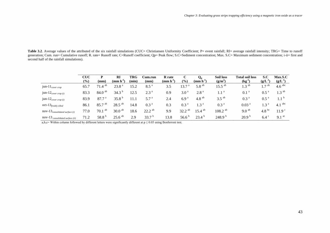
Chapter 3: Evaluating grass strips trapping efficiency using a magnetic iron oxide as a tracer
43
Table 3.2. Average values of the attributed of the six rainfall simulations (CUC= Christiansen Uniformity Coefficient; P= event rainfall; RI= average rainfall intensity; TRG= Time to runoff
generation; Cum. run= Cumulative runoff; R. rate= Runoff rate; C=Runoff coefficient; Qp= Peak flow; S.C=Sediment concentration; Max. S.C= Maximum sediment concentration; i-ii= first and
second half of the rainfall simulations).
CUC
(%)
P
(mm)
RI
(mm h-1
)
TRG
(min)
Cum.run
(mm)
R rate
(mm h-1
)
C
(%)
Qp
(mm h-1
)
Soil loss
(g/m2)
Total soil loss
(kg-1
)
S.C
(g/L-1
)
Max.S.C
(g/L-1
)
jun-11cover crop 65.7 71.4 ab 23.8 a 15.2 8.5 a 3.5 13.7 a 5.8 ab 15.5 ab 1.3 ab 1.7 ab 4.6 abc
jun-12cover crop (i) 83.3 84.0 ab 34.3 b 12.5 2.3 a 0.9 3.0 a 2.8 a 1.1 a 0.1 a 0.5 a 1.3 ab
jun-12cover crop (i) 83.9 87.7 a 35.8 b 11.1 5.7 a 2.4 6.9 a 4.8 ab 3.5 ab 0.3 a 0.5 a 1.1 b
oct-13freshly tilled 86.1 85.7 ab 28.5 ab 14.8 0.3 a 0.3 0.3 a 1.3 a 0.3 a 0.03 a 1.3 a 4.1 abc
nov-13consolidated surface (i) 77.0 70.1 ab 30.0 ab 18.6 22.2 ab 9.9 32.2 ab 15.4 ab 108.2 ab 9.0 ab 4.8 bc 11.9 c
nov-13 consolidated surface (ii) 71.2 58.8 b 25.6 ab 2.9 33.7 b 13.8 56.6 b 23.4 b 248.9 b 20.9 b 6.4 c 9.1 ac
a,b,c= Within column followed by different letters were significantly different at p ≤ 0.05 using Bonferroni test.
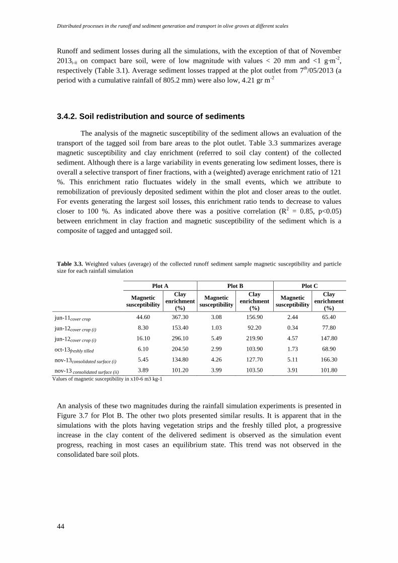
Distributed processes in the runoff and sediment generation and transport in olive groves at different scales
44
Runoff and sediment losses during all the simulations, with the exception of that of November
2013i-ii on compact bare soil, were of low magnitude with values < 20 mm and <1 g·m-2,
respectively (Table 3.1). Average sediment losses trapped at the plot outlet from 7th/05/2013 (a
period with a cumulative rainfall of 805.2 mm) were also low, 4.21 gr m-2
3.4.2. Soil redistribution and source of sediments
The analysis of the magnetic susceptibility of the sediment allows an evaluation of the
transport of the tagged soil from bare areas to the plot outlet. Table 3.3 summarizes average
magnetic susceptibility and clay enrichment (referred to soil clay content) of the collected
sediment. Although there is a large variability in events generating low sediment losses, there is
overall a selective transport of finer fractions, with a (weighted) average enrichment ratio of 121
%. This enrichment ratio fluctuates widely in the small events, which we attribute to
remobilization of previously deposited sediment within the plot and closer areas to the outlet.
For events generating the largest soil losses, this enrichment ratio tends to decrease to values
closer to 100 %. As indicated above there was a positive correlation (R2 = 0.85, p<0.05)
between enrichment in clay fraction and magnetic susceptibility of the sediment which is a
composite of tagged and untagged soil.
Table 3.3. Weighted values (average) of the collected runoff sediment sample magnetic susceptibility and particle
size for each rainfall simulation
Plot A Plot B Plot C
Magnetic
susceptibility
Clay
enrichment
(%)
Magnetic
susceptibility
Clay
enrichment
(%)
Magnetic
susceptibility
Clay
enrichment
(%)
jun-11cover crop 44.60 367.30 3.08 156.90 2.44 65.40
jun-12cover crop (i) 8.30 153.40 1.03 92.20 0.34 77.80
jun-12cover crop (i) 16.10 296.10 5.49 219.90 4.57 147.80
oct-13freshly tilled 6.10 204.50 2.99 103.90 1.73 68.90
nov-13consolidated surface (i) 5.45 134.80 4.26 127.70 5.11 166.30
nov-13 consolidated surface (ii) 3.89 101.20 3.99 103.50 3.91 101.80
Values of magnetic susceptibility in x10-6 m3 kg-1
An analysis of these two magnitudes during the rainfall simulation experiments is presented in
Figure 3.7 for Plot B. The other two plots presented similar results. It is apparent that in the
simulations with the plots having vegetation strips and the freshly tilled plot, a progressive
increase in the clay content of the delivered sediment is observed as the simulation event
progress, reaching in most cases an equilibrium state. This trend was not observed in the
consolidated bare soil plots.
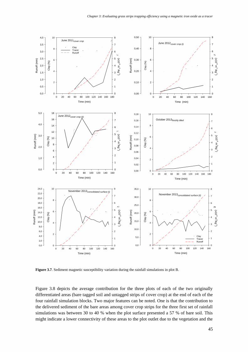
Chapter 3: Evaluating grass strips trapping efficiency using a magnetic iron oxide as a tracer
45
Figure 3.7. Sediment magnetic susceptibility variation during the rainfall simulations in plot B.
Figure 3.8 depicts the average contribution for the three plots of each of the two originally
differentiated areas (bare tagged soil and untagged strips of cover crop) at the end of each of the
four rainfall simulation blocks. Two major features can be noted. One is that the contribution to
the delivered sediment of the bare areas among cover crop strips for the three first set of rainfall
simulations was between 30 to 40 % when the plot surface presented a 57 % of bare soil. This
might indicate a lower connectivity of these areas to the plot outlet due to the vegetation and the
Time (min)
0 20 40 60 80 100 120 140 160
Cla
y (
%)
0
2
4
6
8
10
0
1
2
3
4
5
6
7
8
Ru
no
ff (
mm
)
0,00
0,10
0,20
0,30
0,40
0,50
(x1
0-6 m
3 /kg
-1)
June 2012cover crop (i)
Time (min)
0 20 40 60 80 100 120 140 160 180
Cla
y (
%)
0
2
4
6
8
10
(x10
-6 m3 /k
g-1)
0
1
2
3
4
5
6
7
8R
un
off
(m
m)
0,0
0,5
1,0
1,5
2,0
2,5
3,0
3,5
4,0
Clay
Tracer
Runoff
June 2011cover crop
Time (min)
0 20 40 60 80 100 120 140 160
Cla
y (
%)
0
2
4
6
8
10
12
14
16
18
0
1
2
3
4
5
6
7
8
Ru
no
ff (
mm
)
0,0
1,0
2,0
3,0
4,0
5,0
(x1
0-6 m
3/kg
-1)
June 2012cover crop (ii)
Time (min)
0 20 40 60 80 100 120 140 160 180
Cla
y (
%)
0
2
4
6
8
10
0
1
2
3
4
5
6
7
8
Ru
no
ff (
mm
)
0,00
0,02
0,04
0,06
0,08
0,10
0,12
0,14
0,16
0,18
(x1
0-6 m
3/kg
-1)
October 2013freshly tilled
Time (min)
0 20 40 60 80 100 120 140 160
Cla
y (
%)
0
2
4
6
8
10
0
1
2
3
4
5
6
7
8
Ru
no
ff (
mm
)
0,0
2,0
4,0
6,0
8,0
10,0
12,0
14,0
16,0
18,0
20,0
22,0
24,0
(x1
0-6 m
3/kg
-1)
November 2013consolidated surface (i)
Time (min)
0 20 40 60 80 100 120 140 160
Cla
y (
%)
0
2
4
6
8
10
0
1
2
3
4
5
6
7
8
Ru
no
ff (
mm
)
0,0
5,0
10,0
15,0
20,0
25,0
30,0
35,0
Clay
Tracer
Runoff
(x1
0-6 m
3/kg
-1)
November 2013consolidated surface (ii)
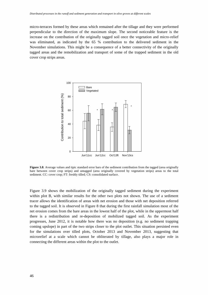
Distributed processes in the runoff and sediment generation and transport in olive groves at different scales
46
micro-terraces formed by these areas which remained after the tillage and they were performed
perpendicular to the direction of the maximum slope. The second noticeable feature is the
increase on the contribution of the originally tagged soil once the vegetation and micro-relief
was eliminated, as indicated by the 65 % contribution to the delivered sediment in the
November simulations. This might be a consequence of a better connectivity of the originally
tagged areas and the remobilization and transport of some of the trapped sediment in the old
cover crop strips areas.
Figure 3.8. Average values and tipic standard error bars of the sediment contribution from the tagged (area originally
bare between cover crop strips) and untagged (area originally covered by vegetation strips) areas to the total
sediment. CC: cover crop; FT: freshly tilled; CS: consolidated surface.
Figure 3.9 shows the mobilization of the originally tagged sediment during the experiment
within plot B, with similar results for the other two plots not shown. The use of a sediment
tracer allows the identification of areas with net erosion and those with net deposition referred
to the tagged soil. It is observed in Figure 8 that during the first rainfall simulation most of the
net erosion comes from the bare areas in the lowest half of the plot, while in the uppermost half
there is a redistribution and re-deposition of mobilized tagged soil. As the experiment
progresses, June 2012, it is notable how there was no deposition (e.g. no sediment trapping
coming upslope) in part of the two strips closer to the plot outlet. This situation persisted even
for the simulations over tilled plots, October 2013 and November 2013, suggesting that
microrelief at a scale which cannot be obliterated by tillage, also plays a major role in
connecting the different areas within the plot to the outlet.
Jun'11cc Jun'12cc Oct'13ft Nov'13cs
Contr
ibution t
o t
ota
l sedim
ent
(%)
0
20
40
60
80
100
Bare
Vegetated
* *
*
Chapter 3: Evaluating grass strips trapping efficiency using a magnetic iron oxide as a tracer
47
Figure 3.9. Soil movement along plot B. Dotted lines show the extension of each vegetation strip. Negative values
denote areas with net soil displacement and positive values areas with net soil deposition.
3.5. Discussion
The measured variability among replicated plots was similar to those observed in
rainfall simulations experiments (Lascelles et al., 2000; Seeger, 2007), or natural rainfall
(Gómez et al., 2001). As expected, there was a large reduction in runoff and sediment losses
from the cover crop strips conditions compared to the bare and tilled ones. Total sediment losses
under cover crop were approximately 50 % of those measured under tilled ones. On the other
hand, cumulative sediment losses under cover crop conditions were approximately 12 % of that
measured under tilled conditions.
Distributed processes in the runoff and sediment generation and transport in olive groves at different scales
48
This reduction in runoff and in sediment losses was similar to the reduction measured by Le
Bissonnais et al. (2004) in a plot experiment with a cover crop strip, of 3 m width, similar to the
ones used in our experiment. Overall the reduction observed is in the range described by many
studies such as Lidgi and Morgan (1995), van Dijk et al. (1996), Martínez et al. (2006) or
Mankin et al. (2007). The reduction in sediment losses is a combination of reduced runoff and
sediment concentration (which in the case of the cover crop strip was approximately 30 % of the
measurements on the tilled plot conditions). The physical processes for this reduction must be
associated to: an increase of infiltration and roughness associated to the cover crop strips
(Römkens and Wang, 1986) and a significant surface storage related with the development of a
micro-terrace by the cover crop strips and to the effects of perpendicular tillage to the direction
of the maximum slope. Abujamin et al. (1988) observed the development of similar induced
bench terraces on the area between the vegetation strips and the sedimentation behind them. All
these results suggest that the evaluated cover crop strips were properly implanted and
performing as expected.
The significant reduction in sediment losses was combined with a significant enrichment of the
delivered sediment. This can be relevant for the evaluation of the effectiveness of the cover
crops as filter strips for agrochemicals, since the carrying capacity for pollutant materials is
related to the size distribution of the eroded material Gabriels and Moldenhauer (1978). Our
study indicates that for the soil type and situations evaluated, there is a trend towards a selective
enrichment of fine particles. This selectivity in the erosion process has been noted by many
studies e.g. Lidgi et al. (1995), Jin and Römkens (2000), Le Bissonais et al. (2004), Malam et al.
(2006), Pan et al. (2010) or Ma et al. (2013). An innovation in this study is the use of a tracer (in
this case magnetic) that can mimic the behavior of agrochemicals that bind to the clay particles
of the soils (case of some fertilizers or herbicides) indicates, and quantifies, these results also in
a selective transport and an increased concentration compared to the original concentration in
soil. Pan et al. (2010) also showed that grass strips were more effective trapping sediments
coarser than 10 or 25 µm. This behavior has not been observed universally in Mediterranean
soils. For instance, Martínez-Mena et al. (1999) showed a preferential enrichment in sand and
silt content on a Lithic Xheric Haploxeroll. Our results are in agreement with independent
measurements on similar soils from different agricultural areas in Andalusia, showing a
selective enrichment in clay and nutrient content in sediment in olive and vineyard growing in
Mediterranean soils using a cover crop compared with a soil management based on bare soil
using tillage (e.g. Gómez et al., 2011). Gómez et al. (2011) indicated how, despite achieving a
drastic reduction in sediment losses using the cover crops compared to tillage, this selective
transport resulted in an increased concentration in nutrients in the sediment coming from the
cover crop treatment compared to the sediment coming from the tilled areas A parallel study
performed in parallel with this rainfall simulation experiment, currently analyzing the results, is
measuring the trapping efficiency of the cover crop strips for several herbicides applied in the
bare soil area, including the implications of this selective transport of finer fractions.
The analysis of the redistribution of the tagged sediment during all the experiments suggest a
large impact of microrelief, and the need of careful traffic and soil management to prevent the
development of areas of preferential flow that can breach the cover crop strips. Stevens and
Quinton (2008) documented by using rare oxide, how tramlines in a field crop area in UK
provide a large connectivity for delivering runoff and sediment downslope out of the field. The
common practice observed in many olive and vineyard growing areas in the Mediterranean of
establishing cover crop strips perpendicular to the direction of the maximum slope (e.g. Gómez
Chapter 3: Evaluating grass strips trapping efficiency using a magnetic iron oxide as a tracer
49
and Giráldez, 2010) but trafficking (for safety or simply convenience) in the direction of the
maximum slope, might result in a drastic reduction of the buffer effectiveness of the cover crops
and should be investigated in more detail. It is interesting to note how the elimination of the
cover crop strips meant the remobilization and delivered to the plot outlet of a large fraction of
the tagged soil. This implies that temporal elimination of the cover crop strips, which is an
operation sometime uses rather to seed a new cover crop or to remove this during the dry season
in tree crops in Southern Spain can cause a severe decrease of trapping effects of cover crop if
an storm occurs during the summer or early fall period (which is not uncommon in the
Mediterranean type of climate) prior to the development of a new cover. This kind of
management should also be discouraged, and when necessary the replacement of the cover crop
should be made partially leaving some of the strips in place to prevent catastrophic events such
as the simulated in the tilled conditions of our experiment.
3.6. Conclusions
Rainfall simulations under different soil conditions combined with the analysis of
sediment particle size and redistribution movement using magnetic iron oxide as sediment tracer
have demonstrated to be a useful methodology for determining vegetation strips behavior at plot
scale in comparison with tilled bare soil. Our results indicate that when using cover crops strips,
runoff and sediment losses were, respectively, approximately 50 and 12 % of that measured
when the plot was completely bare and tilled. This reduction was related with increased
infiltration, higher hydraulic and topographic roughness induced by the vegetation, and
development of a micro-terrace where the cover crop strip was. There was a selective transport
of clay particle size in the sediment leaving the plots associated with preferential transport of the
substances, as the magnetic tracer indicated. Therefore, a great quantity of agrochemicals
movement, with preferential binding to the clay particles, is expected. This can explain the trend
observed in other experiments in Mediterranean areas, with similar soils for an increase
concentration of some nutrients in the sediment leaving cover crop treatments, in comparison to
bare soil in olive and vineyards.
Acknowledgements
The authors would like to thank Clemente Trujillo, Manuel Redondo and Azahara Ramos
for their full help and support during the fieldwork. This study was supported by the Project
P08-AGR-03925 (Andalusian Government), AGL2009-12936-C03-01 (Ministry of Science and
Innovation), RESEL (Ministry of Agriculture, Food and Environment) and FEDER fund. The
program JAE of the National Spanish Research Centre which provided grant support for the
PhD project of the corresponding author is also thanked.

Distributed processes in the runoff and sediment generation and transport in olive groves at different scales
50
Chapter 4: Exploring calibration strategies of SEDD model in two olive orchard watersheds
51
Chapter 4
Exploring calibration strategies of
SEDD model in two olive orchard watersheds
Part of the results of this chapter has been presented as a communication in:
European Geoscience Union, EGU (2012):
Burguet, M., Taguas, E.V., Gómez, J.A.: Estimating soil losses in two Mediterranean
olive catchments using SEDD model Geoscience Union, EGU, 2012.
Submitted to Geomorphology.
‘Water is the driver of Nature’
Leonardo da Vinci (1452-1519)

Distributed processes in the runoff and sediment generation and transport in olive groves at different scales
52
Chapter 4: Exploring calibration strategies of SEDD model in two olive orchard watersheds
53
Resumen
La optimización de las estrategias de conservación de suelo, requiere un diagnóstico
apropiado de las principales fuentes contribuyentes a la degradación de suelo en el proceso de
identificación de las áreas prioritarias para la implentación de dichas estrategias. En este
estudio, se exploraron distintas estrategias de calibración del modelo SEDD en dos olivares
comerciales de 6.7 (Setenil) y 8 ha (Conchuela) situados en España, los cuales han estado
monitorizados por un periodo de 6 años. En Setenil se midieron un total de 121 eventos,
mientras que en el caso de Conchuela 195. Los principales objetivos de este trabajo fueron: [1]
calibrar el modelo en las cuencas de estudio con distintas características ambientales y manejos
de suelo distintos, [2] estudiar diferentes estrategias de calibración y parametrización para
facilitar el uso del modelo bajo diferentes condiciones de escorrentía y [3], evaluar la
variabilidad temporal del coeficiente de entrega de sedimento (SDR) a escala de evento y anual
para, de esta forma, determinar qué áreas dentro de la cuenca contribuyen a la mayor
exportación de sedimento y, de esta forma, concentrar las diferentes medidas de conservación.
El valor de β es el principal parámetro del modelo que representa el peso de los tiempos de viaje
de las distintas unidades geomorfológicas de la cuenca. Para la calibración de SEDD se
representaron cinco escenarios diferentes de erosividad que combinaban distintas ponderaciones
de las componentes de lluvia y del flujo. Asimismo se evaluó el efecto de valores únicos y
quincenales del factor de manejo (C) con el fin de optimizar el esfuerzo en calibración. En este
caso, se calcularon valores de C-RUSLE anuales (de 0.50 a 0.01 con un intervalo de 5) los
cuales se asociaron al tipo de manejo de suelo, y valores de C-RUSLE estacionales derivados de
la humedad del suelo y la cubierta espontánea. El mejor escenario para Setenil (Rt=Rp) se asoció
a una erosividad total igual a la erosividad asociada a la lluvia. Por el contrario, el mejor
escenario para Conchuela estuvo asociado a los valores de erosividad equivalentes a la
erosividad dependiente del flujo (escorrentía y caudal punta, Rt=Rq). La mediana de la
distribución de los valores de β de los eventos proporcionó un buen ajuste del modelo
únicamente en Conchuela con C-RUSLE anual (E=0.92, RMSE=4.78 para C-RUSLE=0.30). En
el caso de Setenil, el análisis de la función del coeficiente de entrega (dependiente de β) justificó
el agrupar los eventos de acuerdo al signo de β, lo cual proporcionó un aceptable ajuste cuando
las medianas de cada región (positiva y negativa) fueran usadas (E=0.58, RMSE=7.94 para C-
RUSLE=0.30). Finalmente, el uso de C estacionales mejoró la calibración, particularmente en
Conchuela (E=0.95, RMSE=5.03) donde los efectos de la humedad asociados al suelo (Vertisol)
son significativos.
Los coeficientes de entrega de sedimento (SDR) en ambas cuencas indican un transporte de
sedimento muy dinámico. El SDR medio anual en Setenil fue de 64.1 % (con una desviación
estándar de 57.5 %), mientras que en Conchuela fue de 94.2 % (con una desviación estándar de
83.7 %). Los valores extremos de SDR (>100 %) se asociaron a años muy húmedos con valores
de precipitación un 30 % mayores que la media. A escala de evento, se observaron tendencias
simulares y los SDR> 100% se asociaron a un papel dominante en la exportación de sedimentos
de cárcavas en Conchuela y de regueros y cárcava efímera en Setenil.
Palabras clave: SEDD, SDR, RUSLE, unidad geomorfológica, microcuenca olivarera
Distributed processes in the runoff and sediment generation and transport in olive groves at different scales
54
Abstract
In order to optimize soil conservation strategies, an accurate diagnosis of the main areas
contributing to soil erosion in catchments which can be identified through models such as
SEDD (Sediment Delivery Distributed model) is required. In this study, different calibration
strategies of the SEDD model were explored in two commercial olive microcatchments, both
located in Spain - Setenil (6.7 ha) and Conchuela (8 ha) - and monitored for a 6-year period. The
main objectives were: [1] to calibrate the model to study watersheds with different
environmental characteristics and different soil management, [2] to study different calibration
and parameterization strategies in order to facilitate use of the model under different runoff
conditions, and [3] to evaluate the temporal variability of the sediment delivery ratio (SDR) at
the event and annual scale. This last objective could enable us to determine which areas within
the watershed are contributing to sediment export and, thus, choose the ideal soil conservation
strategies in those areas.
For SEDD calibration, five different erosivity scenarios were represented. In these scenarios,
combinations of different weights of precipitation components and concentrated flow were
explored. Furthermore, in order to optimize the calibration, biweekly and annual C-RUSLE
values were evaluated. In all these scenarios, the analysis was focused on β, which represents
the weight of the travel times of the different watershed geomorphological units, as the main
model parameter.
The SEDD model was calibrated successfully in the Conchuela watershed, whereas poor
adjustments were found for the Setenil watershed, due to the adjustment of the β-median. In
Conchuela, the best calibration scenarios were associated with erosivity values related to
concentrated flow, while the erosivity value for the Setenil watershed was only rain-dependent.
Biweekly C-RUSLE values provided suitable, consistent results in Conchuela where there tends
to be considerable variability in soil moisture over the year. In contrast, there were no
appreciable improvements between annual and biweekly C-RUSLE values in Setenil, probably
due to the narrower variation interval.
The analysis of the SDR function justified the grouping of the different β values according to
their sign (positive or negative) as a calibration strategy in Setenil. The medians of these groups
of events allowed them to be adjusted (E = 0.7; RMSE= 6.4). In the Conchuela watershed, this
variation in the model calibration produced only minor improvements to an adjustment which
was already good.
The sediment delivery ratios (SDR) in both watersheds indicate very dynamic sediment
transport. The mean annual SDR for Setenil was 64.1 % (with a standard deviation of 57.5 %),
while in Conchuela it was 110.1 % (with a standard deviation of 83.7 %). Extreme SDR values
(>100 %) were associated with very humid years and with precipitations 30 % above the mean
values. At the event scale, similar SDR behaviour was observed. SDR values >100 % were
associated with a dominant role of the gully in exporting sediments out of the watershed in
Conchuela, whereas this was done by rills and an ephemeral gully in the Setenil watershed.
Keywords: SEDD, SDR, RUSLE, geomorphological unit, olive microcatchment
Chapter 4: Exploring calibration strategies of SEDD model in two olive orchard watersheds
55
4.1. Introduction
Olive plantations located in mountainous areas or on steep slopes in Southern Spain
have been identified as one of the major sources of soil erosion in the region (Gómez-Limón et
al. 2011). In work carried out by Vanwalleghem et al., (2011), reconstructing the temporal
variation of soil management and its erosion rates in olive trees located in mountainous areas,
the authors found soil losses of between 8 and 124 t ha-1 year-1 for water treatment and soil
losses from 3 up to 42 t ha-1 year-1 for tillage management (similar to values obtained by Gómez
et al., 2009). A number of experimental studies have been performed to quantify soil losses in
olive orchards and to evaluate the impact of different managements in runoff plots with a
maximum size of 200 m2 (Kosmas et al., 1997; Pastor et al., 1999; Gómez et al.,
2003;2004;2009; Licciardello et al., 2013). In a summary of their experimental studies, Gómez
et al. (2008) indicated how at the hillslope scale, the soil management of olive orchards with
bare soil resulted in unsustainable water erosion rates when measured in plots of adequate
length to represent hillslope processes. At this spatial scale, the erosive processes taking place
are mainly splash, inter-rill and rill erosion; however, on commercial farms, there can also be
major erosion derived from concentrated flow in larger rills or gullies. For instance, Taguas and
Gómez (2015) measured total soil losses of >10 t ha-1 year-1 in a hilly olive microcatchment
with a mean slope of 9.5 % in Southern Spain for hydrological years with annual precipitation
close to the long-term average (700 mm). Thus, studies of soil losses from geomorphologic
units such as micro-watersheds (Taguas et al., 2009; 2010; Gómez et al., 2014), can provide
information which is more relevant to the challenges faced by farmers in implementing suitable
management measures to ensure the sustainability of resources and safeguard their incomes.
In order to optimize conservation strategies, an accurate diagnosis of the main sediment sources
contributing to soil erosion is required, as well as identifying the areas where the measures
should be implemented more urgently. Locating and determining the morphological origins of
the sediment will help us to predict which areas are more prone to soil loss and which type of
soil conservation measure is more suitable (vegetation strips, check dams, afforestation in
rivers, etc).
Research carried out over the last 50 years has developed erosion models which can predict
sediment production at different spatial and temporal scales, as well as performing specific
monitoring of the different erosive processes in different regions of the world (a review of the
different models applied in soil erosion studies can be found in Merrit et al., 2003). Erosion
models can help us to understand hydrological processes, and simple parametric approximations
such as USLE (Universal Soil Loss Equation; Wischmeier and Smith, 1978) or its revised
version RUSLE (Renard et al., 1997), calibrated from physical parameters, are commonly used
to evaluate risk of soil erosion all around the world.
SEDD (Ferro and Minacapilly, 1995) is a sediment delivery distributed model based on the
USLE whose main features are its applicability at the scale of the geomorphological units into
which a basin is divided, and the ability to predict SDR at the geomorphological unit and
catchment scale (Ferro and Porto, 2000). Using the USLE as a starting point, the model has
been calibrated under different environments (from studies in the Mediterranean basin, the
Pyrenees and Northwest USA) and soil managements such as eucalyptus forests (Ferro and
Porto, 2000); coniferous forests with croplands (Fernández et al., 2003; Fu et al., 2006; López-
Vicente and Navas, 2011), olive watersheds (Taguas et al., 2011) and naturally-colonized
abandoned farms (López-Vicente et al., 2013). It has been also validated with Cs137 in forested
Distributed processes in the runoff and sediment generation and transport in olive groves at different scales
56
areas with eucalyptus trees at the mean annual temporal scale. In this study, the model was
applied at both geomorphological unit and basin scales (Di Stefano et al., 2005). The SEDD
model was chosen for our study because: (1) it allows for discretization of a watershed into
geomorphological units; (2) it predicts SDR at the geomorphological unit and basin scales; (3) it
is based on the RUSLE, a model used under Mediterranean olive catchments with favourable
results (Gómez et al., 2003; Vanwalleghem et al., 2011); (4) it is easy to couple within a GIS
(López-Vicente and Navas, 2010); (5) previous studies performed in olive catchments in south
Spain support its application and reliability (Taguas et al., 2011).
The present work aims to shed light on watershed scale erosion studies in commercial olive
farms, by adapting tools to evaluate soil degradation risk. The specific objectives were then [1]
to calibrate the model on two different commercial farms with olive cultivations located in areas
with different environmental features in terms of precipitation, soils and management, and
monitored over a period of six years; [2] to study different calibration strategies and
parameterisation in order to facilitate the use of the model in different conditions and [3] to
evaluate the temporal variability of Sediment Delivery Ratios (SDRs) at the event and the
annual scales, identify the areas which contribute most to the soil losses and decide where the
conservation measures should be concentrated.
4.2. Study site and available data
4.2.1. Catchment location and description
Two commercial olive microcatchments were selected for this study (Fig. 1). The
Setenil microcatchment is located in the province of Cádiz (36.88º N, 5.13º W). The drainage
area is 6.7 ha, with a mean elevation of 782 m and mean slope of 9.5 %. A full description of
the watershed can be found in Taguas and Gómez, (2015). A total of six hydrological years
under different soil management techniques were used in the analysis. In 2005-2006 and 2006-
2007, the soil management applied was no tillage (NT), with bare soil and using herbicide;
conventional tillage (CT) was used in 2007-08, 2008-09 and 2009-10 and conservation
measures (CM) which included mulching were applied in 2010-11. A summary of the soil
management operations conducted in the Setenil catchment was published by Taguas and
Gómez, (2015).
The experimental catchment of 'La Conchuela' (37º N, 4º W) is located 10 km west of Cordoba.
The drainage area is 8 ha, with a mean elevation of 142 m and mean slope of 9 %. The soil
management technique used was growing natural weed vegetation in the lanes, applying
glyphosate and occasional mowing in some areas. At the same time, surface tillage was
occasionally used, but only to cover rills or small gullies so tractors could pass (Gómez et al.,
2014). A total of five hydrological years were used in the analysis. As in Setenil, a complete
description of the watershed and its measuring equipment can be found in Gómez et al., (2014).
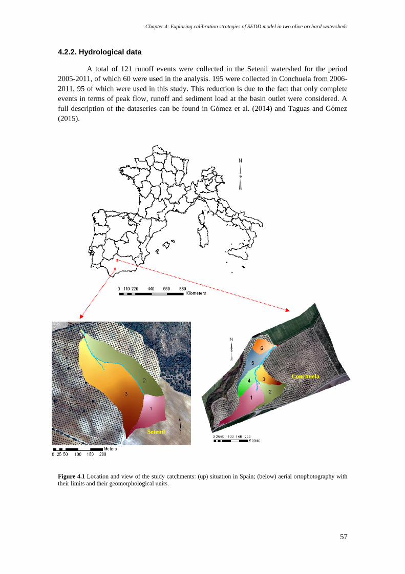
Chapter 4: Exploring calibration strategies of SEDD model in two olive orchard watersheds
57
4.2.2. Hydrological data
A total of 121 runoff events were collected in the Setenil watershed for the period
2005-2011, of which 60 were used in the analysis. 195 were collected in Conchuela from 2006-
2011, 95 of which were used in this study. This reduction is due to the fact that only complete
events in terms of peak flow, runoff and sediment load at the basin outlet were considered. A
full description of the dataseries can be found in Gómez et al. (2014) and Taguas and Gómez
(2015).
Figure 4.1 Location and view of the study catchments: (up) situation in Spain; (below) aerial ortophotography with
their limits and their geomorphological units.
Setenil
Conchuela
Distributed processes in the runoff and sediment generation and transport in olive groves at different scales
58
4.3. Methods
4.3.1. SEDD model (Sediment Delivery Distributed model)
4.3.1.1. Model components
SEDD (Sediment Delivery Distributed model) is a distributed model developed to
calculate sediment yield based on the USLE (or its revised version RUSLE) and the SDR
calculations for each geomorphological unit i (SDRi).
SDRi depends on the eroded particle travel time along the hydraulic path until it reaches the
nearest channel, after which it becomes a variable subrogated to travel time. Ferro and
Minacapilli (1995) established an equation (1) to calculate the sediment delivery ratio for each
geomorphological unit (SDRi):
,exp( )i p iSDR t [1]
where ,p it is the travel time (m) for each geomorphological unit, and β (m-1) is a coefficient
(assumed constant for the basin) according to the calculated linear relationship between the
logarithm of the cumulative frequency of length and the square root of the slope of the hydraulic
path, and the travel time (Ferro and Porto, 1998). The travel time of the eroded particles in each
geomorphological unit (,p it ) is calculated as in equation (2):
, ,
,
1, ,
pN
p i i j
p i
jp i i j
lt
S S
[2]
where ,p il and
,i j (m) are the length of each geomorphological unit i located along the
hydraulic path, and ,p iS (m m-1) is the slope of the hydraulic path along each geomorphological
unit i. In this study, the slope was calculated as in Laurenson (1986).
Equation (1) can be rewritten to take into account both the calculation of SDRi and the travel
time for each geomorphological unit, as in equation (3):
, ,
,
1, ,
exp exp exppN
p i i j
i p i
jp i i j
lSDR t
S S
[3]
Some authors have tried different values for β (described as the median value and assumed
constant for the calculations according to Ferro and Minacapilli, 1995) without it being directly
solved from the equation, and then using the value which gave a better approximation (e.g.
increments of 0.1 in the case of Jain and Kothyari, 2000, or assuming β with a constant value as
in Fu et al., 2006 and López-Vicente and Navas, 2010, López-Vicente et al., 2011). In this
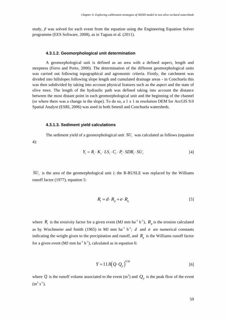
Chapter 4: Exploring calibration strategies of SEDD model in two olive orchard watersheds
59
study, β was solved for each event from the equation using the Engineering Equation Solver
programme (EES Software, 2008), as in Taguas et al. (2011).
4.3.1.2. Geomorphological unit determination
A geomorphological unit is defined as an area with a defined aspect, length and
steepness (Ferro and Porto, 2000). The determination of the different geomorphological units
was carried out following topographical and agronomic criteria. Firstly, the catchment was
divided into hillslopes following slope length and cumulated drainage areas - in Conchuela this
was then subdivided by taking into account physical features such as the aspect and the state of
olive trees. The length of the hydraulic path was defined taking into account the distance
between the most distant point in each geomorphological unit and the beginning of the channel
(or where there was a change in the slope). To do so, a 1 x 1 m resolution DEM for ArcGIS 9.0
Spatial Analyst (ESRI, 2006) was used in both Setenil and Conchuela watersheds.
4.3.1.3. Sediment yield calculations
The sediment yield of a geomorphological unit iSU was calculated as follows (equation
4):
ï i i i i i i iY R K LS C P SDR SU [4]
iSU is the area of the geomorphological unit i; the R-RUSLE was replaced by the Williams
runoff factor (1977), equation 5:
t p qR d R e R [5]
where tR is the erosivity factor for a given event (MJ mm ha-1 h-1), pR is the erosion calculated
as by Wischmeier and Smith (1965) in MJ mm ha-1 h-1; d and e are numerical constants
indicating the weight given to the precipitation and runoff, and qR is the Williams runoff factor
for a given event (MJ mm ha-1 h-1), calculated as in equation 6:
0.56
11.8 pY Q Q [6]
where Q is the runoff volume associated to the event (m3) and pQ is the peak flow of the event
(m3 s-1).

Distributed processes in the runoff and sediment generation and transport in olive groves at different scales
60
LS-RUSLE represents the proportion of soil loss for a given length and slope. To determine the
value of the longitude and slope, a 1 x 1 m resolution DEM was obtained in 2011 for both
basins. The topographic factor was calculated following the Moore and Burch (1986) approach
(equation 7):
0.4 1.3sin
( 1)22.13 0.0896
sALS n
[7]
where sA represents the slope length expressed as the drainage area per unit area (m2 m-1),
obtained with the 'flow accumulation' function, which calculates the number of cells upstream
(Arctoolbox, Hydrology functions, ESRI, 2009); n =0.4 and δ (º) is the DEM cell slope
(Taguas et al., 2011).
C-RUSLE reflects the effect of the crop and soil management on the erosion rates. It varies
depending on the soil management and the state of the soil in the catchment, particularly soil
moisture and ground cover by vegetation and crop residues, and it was calculated as indicated in
section 2.3.4.
When calculating K-RUSLE, a total of 13 soil samples were collected in the Setenil watershed
below the tree canopy and in the tree rows at a depth of 10 cm and the location was stored in a
GPS. Soil texture was obtained by the pipette method, organic matter content by the Walkley-
Black method and percentage of carbonates by the van Wesemael method (Taguas, 2007).
Similarly, 45 soil samples were also taken below the tree canopy and in the tree rows at a depth
of 5 cm in the Conchuela watershed. The M factor was calculated taking into account the
percentage of clay, silt and fine sand. The K-RUSLE was then calculated according to Renard et
al., (1997). The K-RUSLE for each watershed was then calculated using an Inverse Distance
Weight (IDW) interpolation method coupled to the ArcGIS Spatial Analyst (ESRI, 2009).
In this work, a value of P-RUSLE equal to 1 was used.
Thus, the basin sediment production would be the sum of the sediment yield of each
geomorphological unit in which the basin is divided, as in equation 8 (Ferro and Porto, 2000):
,exppN
b t b i i i p i i
i j
Y R C K LS P t SU
[8]
Average potential erosion was calculated following the RUSLE (Renard et al., 1997) equation
(with RUSLE factors calculated as mentioned above) and was only computed with an
established threshold value of daily precipitation >10 mm for each event and for each
geomorphological unit.
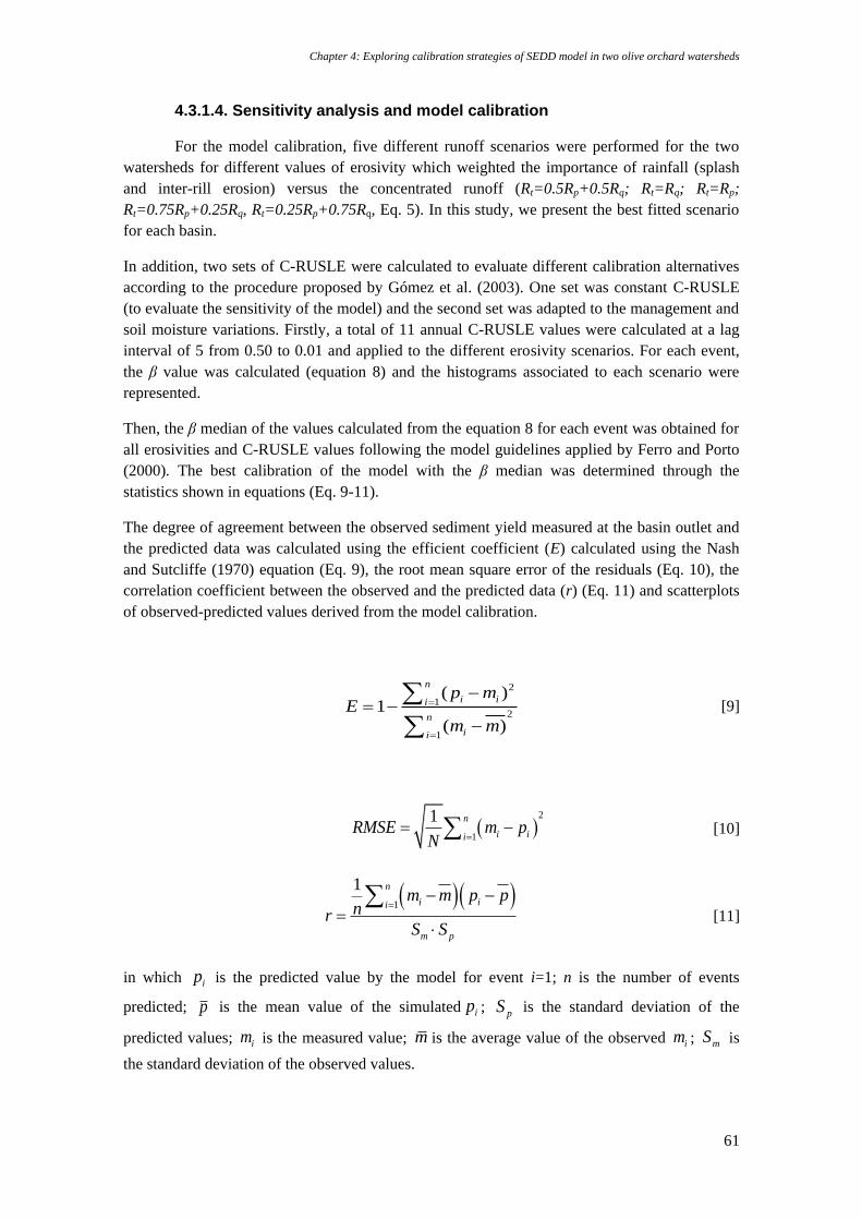
Chapter 4: Exploring calibration strategies of SEDD model in two olive orchard watersheds
61
4.3.1.4. Sensitivity analysis and model calibration
For the model calibration, five different runoff scenarios were performed for the two
watersheds for different values of erosivity which weighted the importance of rainfall (splash
and inter-rill erosion) versus the concentrated runoff (Rt=0.5Rp+0.5Rq; Rt=Rq; Rt=Rp;
Rt=0.75Rp+0.25Rq, Rt=0.25Rp+0.75Rq, Eq. 5). In this study, we present the best fitted scenario
for each basin.
In addition, two sets of C-RUSLE were calculated to evaluate different calibration alternatives
according to the procedure proposed by Gómez et al. (2003). One set was constant C-RUSLE
(to evaluate the sensitivity of the model) and the second set was adapted to the management and
soil moisture variations. Firstly, a total of 11 annual C-RUSLE values were calculated at a lag
interval of 5 from 0.50 to 0.01 and applied to the different erosivity scenarios. For each event,
the β value was calculated (equation 8) and the histograms associated to each scenario were
represented.
Then, the β median of the values calculated from the equation 8 for each event was obtained for
all erosivities and C-RUSLE values following the model guidelines applied by Ferro and Porto
(2000). The best calibration of the model with the β median was determined through the
statistics shown in equations (Eq. 9-11).
The degree of agreement between the observed sediment yield measured at the basin outlet and
the predicted data was calculated using the efficient coefficient (E) calculated using the Nash
and Sutcliffe (1970) equation (Eq. 9), the root mean square error of the residuals (Eq. 10), the
correlation coefficient between the observed and the predicted data (r) (Eq. 11) and scatterplots
of observed-predicted values derived from the model calibration.
2
1
2
1
( )1
( )
n
i ii
n
ii
p mE
m m
[9]
2
1
1 n
i iiRMSE m p
N [10]
1
1 n
i ii
m p
m m p pnr
S S
[11]
in which ip is the predicted value by the model for event i=1; n is the number of events
predicted; p is the mean value of the simulated ip ; pS is the standard deviation of the
predicted values; im is the measured value; m is the average value of the observed im ; mS is
the standard deviation of the observed values.
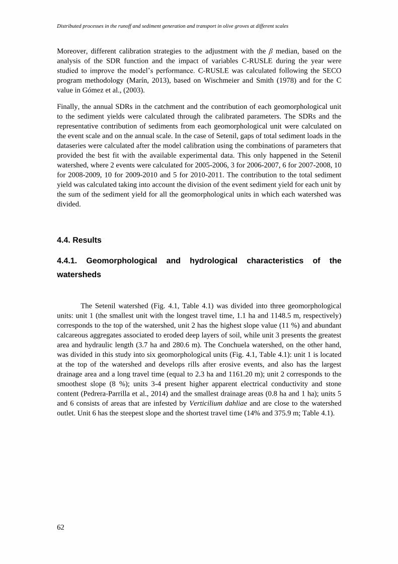
Distributed processes in the runoff and sediment generation and transport in olive groves at different scales
62
Moreover, different calibration strategies to the adjustment with the β median, based on the
analysis of the SDR function and the impact of variables C-RUSLE during the year were
studied to improve the model’s performance. C-RUSLE was calculated following the SECO
program methodology (Marín, 2013), based on Wischmeier and Smith (1978) and for the C
value in Gómez et al., (2003).
Finally, the annual SDRs in the catchment and the contribution of each geomorphological unit
to the sediment yields were calculated through the calibrated parameters. The SDRs and the
representative contribution of sediments from each geomorphological unit were calculated on
the event scale and on the annual scale. In the case of Setenil, gaps of total sediment loads in the
dataseries were calculated after the model calibration using the combinations of parameters that
provided the best fit with the available experimental data. This only happened in the Setenil
watershed, where 2 events were calculated for 2005-2006, 3 for 2006-2007, 6 for 2007-2008, 10
for 2008-2009, 10 for 2009-2010 and 5 for 2010-2011. The contribution to the total sediment
yield was calculated taking into account the division of the event sediment yield for each unit by
the sum of the sediment yield for all the geomorphological units in which each watershed was
divided.
4.4. Results
4.4.1. Geomorphological and hydrological characteristics of the
watersheds
The Setenil watershed (Fig. 4.1, Table 4.1) was divided into three geomorphological
units: unit 1 (the smallest unit with the longest travel time, 1.1 ha and 1148.5 m, respectively)
corresponds to the top of the watershed, unit 2 has the highest slope value (11 %) and abundant
calcareous aggregates associated to eroded deep layers of soil, while unit 3 presents the greatest
area and hydraulic length (3.7 ha and 280.6 m). The Conchuela watershed, on the other hand,
was divided in this study into six geomorphological units (Fig. 4.1, Table 4.1): unit 1 is located
at the top of the watershed and develops rills after erosive events, and also has the largest
drainage area and a long travel time (equal to 2.3 ha and 1161.20 m); unit 2 corresponds to the
smoothest slope (8 %); units 3-4 present higher apparent electrical conductivity and stone
content (Pedrera-Parrilla et al., 2014) and the smallest drainage areas (0.8 ha and 1 ha); units 5
and 6 consists of areas that are infested by Verticilium dahliae and are close to the watershed
outlet. Unit 6 has the steepest slope and the shortest travel time (14% and 375.9 m; Table 4.1).
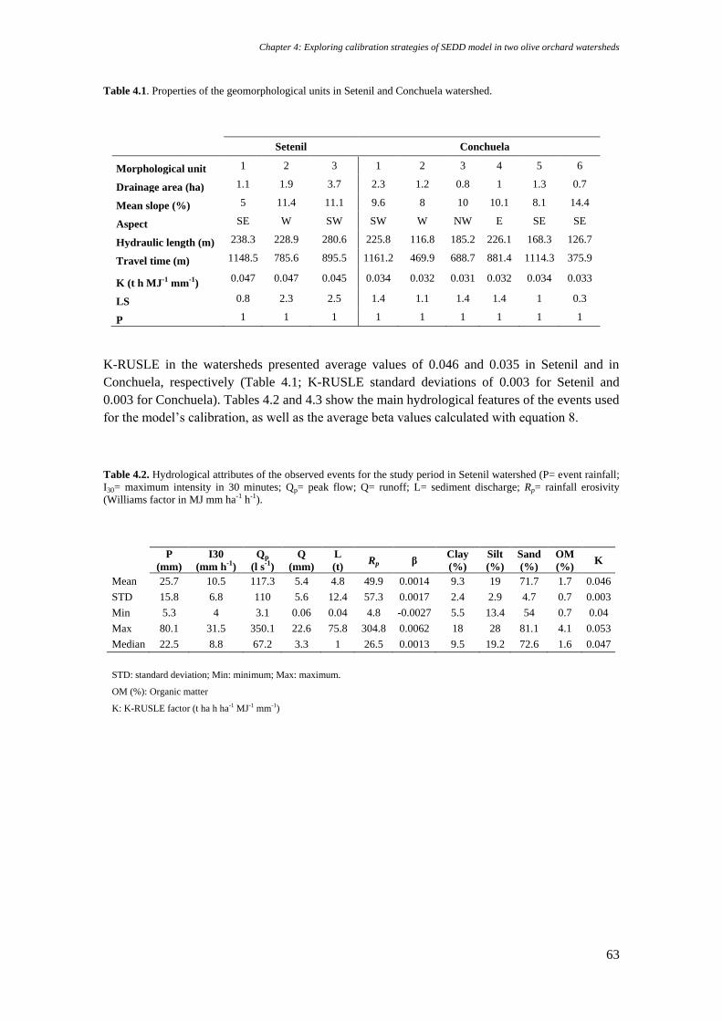
Chapter 4: Exploring calibration strategies of SEDD model in two olive orchard watersheds
63
Table 4.1. Properties of the geomorphological units in Setenil and Conchuela watershed.
Setenil Conchuela
Morphological unit 1 2 3 1 2 3 4 5 6
Drainage area (ha) 1.1 1.9 3.7 2.3 1.2 0.8 1 1.3 0.7
Mean slope (%) 5 11.4 11.1 9.6 8 10 10.1 8.1 14.4
Aspect SE W SW SW W NW E SE SE
Hydraulic length (m) 238.3 228.9 280.6 225.8 116.8 185.2 226.1 168.3 126.7
Travel time (m) 1148.5 785.6 895.5 1161.2 469.9 688.7 881.4 1114.3 375.9
K (t h MJ-1
mm-1
) 0.047 0.047 0.045 0.034 0.032 0.031 0.032 0.034 0.033
LS 0.8 2.3 2.5 1.4 1.1 1.4 1.4 1 0.3
P 1 1 1 1 1 1 1 1 1
K-RUSLE in the watersheds presented average values of 0.046 and 0.035 in Setenil and in
Conchuela, respectively (Table 4.1; K-RUSLE standard deviations of 0.003 for Setenil and
0.003 for Conchuela). Tables 4.2 and 4.3 show the main hydrological features of the events used
for the model’s calibration, as well as the average beta values calculated with equation 8.
Table 4.2. Hydrological attributes of the observed events for the study period in Setenil watershed (P= event rainfall;
I30= maximum intensity in 30 minutes; Qp= peak flow; Q= runoff; L= sediment discharge; Rp= rainfall erosivity
(Williams factor in MJ mm ha-1 h-1).
P
(mm)
I30
(mm h-1
)
Qp
(l s-1
)
Q
(mm)
L
(t) Rp β
Clay
(%)
Silt
(%)
Sand
(%)
OM
(%) K
Mean 25.7 10.5 117.3 5.4 4.8 49.9 0.0014 9.3 19 71.7 1.7 0.046
STD 15.8 6.8 110 5.6 12.4 57.3 0.0017 2.4 2.9 4.7 0.7 0.003
Min 5.3 4 3.1 0.06 0.04 4.8 -0.0027 5.5 13.4 54 0.7 0.04
Max 80.1 31.5 350.1 22.6 75.8 304.8 0.0062 18 28 81.1 4.1 0.053
Median 22.5 8.8 67.2 3.3 1 26.5 0.0013 9.5 19.2 72.6 1.6 0.047
STD: standard deviation; Min: minimum; Max: maximum.
OM (%): Organic matter
K: K-RUSLE factor (t ha h ha-1 MJ-1 mm-1)
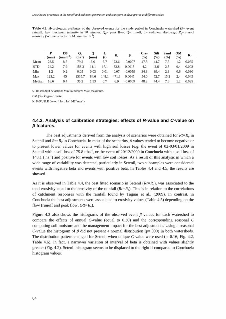
Distributed processes in the runoff and sediment generation and transport in olive groves at different scales
64
Table 4.3. Hydrological attributes of the observed events for the study period in Conchuela watershed (P= event
rainfall; I30= maximum intensity in 30 minutes; Qp= peak flow; Q= runoff; L= sediment discharge; Rq= runoff
erosivity (Williams factor in MJ mm ha-1 h-1).
P
(mm)
I30
(mm h-1
)
Qp
(l s-1
)
Q
(mm)
L
(t) Rq β
Clay
(%)
Silt
(%)
Sand
(%)
OM
(%) K
Mean 23.5 8.6 79.2 6.0 6.7 23.6 -0.0007 47.8 44.7 7.5 1.2 0.035
STD 24.2 7.9 153.3 11.1 17.1 53.8 0.0015 4.2 2.6 2.5 0.4 0.003
Min 1.2 0.2 0.05 0.03 0.01 0.07 -0.0059 34.3 39.4 2.3 0.6 0.030
Max 123.2 45 1335.7 84.6 148.1 471.3 0.0045 54.0 52.7 15.2 2.4 0.045
Median 16.6 6.4 35.2 1.53 0.7 6.9 -0.0009 48.2 44.4 7.6 1.2 0.035
STD: standard deviation; Min: minimum; Max: maximum.
OM (%): Organic matter
K: K-RUSLE factor (t ha h ha-1 MJ-1 mm-1)
4.4.2. Analysis of calibration strategies: effects of R-value and C-value on β features.
The best adjustments derived from the analysis of scenarios were obtained for Rt=Rp in
Setenil and Rt=Rq in Conchuela. In most of the scenarios, β values tended to become negative or
to present lower values for events with high soil losses (e.g. the event of 02-03/01/2009 in
Setenil with a soil loss of 75.8 t ha-1, or the event of 20/12/2009 in Conchuela with a soil loss of
148.1 t ha-1) and positive for events with low soil losses. As a result of this analysis in which a
wide range of variability was detected, particularly in Setenil, two subsamples were considered:
events with negative beta and events with positive beta. In Tables 4.4 and 4.5, the results are
showed.
As it is observed in Table 4.4, the best fitted scenario in Setenil (Rt=Rp), was associated to the
total erosivity equal to the erosivity of the rainfall (Rt=Rp). This is in relation to the correlations
of catchment responses with the rainfall found by Taguas et al., (2009). In contrast, in
Conchuela the best adjustments were associated to erosivity values (Table 4.5) depending on the
flow (runoff and peak flow; (Rt=Rq).
Figure 4.2 also shows the histograms of the observed event β values for each watershed to
compare the effects of annual C-value (equal to 0.30) and the corresponding seasonal C
computing soil moisture and the management impact for the best adjustments. Using a seasonal
C-value the histogram of β did not present a normal distribution (p=.000) in both watersheds.
The distribution pattern changed for Setenil when unique C-value were used (p=0.16; Fig. 4.2,
Table 4.6). In fact, a narrower variation of interval of beta is obtained with values slightly
greater (Fig. 4.2). Setenil histogram seems to be displaced to the right if compared to Conchuela
histogram values.
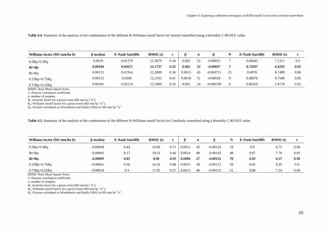
Chapter 4: Exploring calibration strategies of SEDD model in two olive orchard watersheds
65
Table 4.4. Summary of the analysis of the combination of the different R-Williams runoff factor for Setenil watershed using a biweekly C-RUSLE value.
Williams factor (MJ mm/ha h) β median E-Nash-Sutcliffe RMSE (t) r β+ n β
- N E-Nash-Sutcliffe RMSE (t) r
0.5Rp+0.5Rq 0.0018 0.01279 12.2679 0.34 0.002 53 -0.00055 7 0.66643 7.1311 0.9
Rt=Rp 0.00184 0.02671 12.1737 0.25 0.002 53 -0.00037 7 0.72937 6.4193 0.91
Rt=Rq 0.00115 0.02354 12.2009 0.36 0.0015 45 -0.000711 15 0.4978 8.7499 0.86
0.25Rp+0.75Rq 0.00153 0.0206 12.2193 0.41 0.0018 51 -0.00034 9 0.49676 8.7589 0.85
0.75Rp+0.25Rq 0.00181 0.02514 12.1909 0.29 0.002 54 -0.000709 6 0.80359 5.4719 0.93
RMSE: Root Mean Square Error.
r= Pearson correlation coefficient.
n: number of samples.
Rt: erosivity factor for a given event (MJ mm ha-1 h-1).
Rq: Williams runoff factor for a given event (MJ mm ha-1 h-1).
Rp: Erosion calculated as Wischmeier and Smith (1965) in MJ mm ha-1 h-1.
Table 4.5. Summary of the analysis of the combination of the different R-Williams runoff factor for Conchuela watershed using a biweekly C-RUSLE value.
Williams factor (MJ mm/ha h) β median E-Nash-Sutcliffe RMSE (t) r β+ n β
- N E-Nash-Sutcliffe RMSE (t) r
0.5Rp+0.5Rq -0.00028 0.44 16.09 0.71 0.0012 43 -0.00124 54 0.9 6.75 0.96
Rt=Rp -0.00001 0.17 19.52 0.46 0.0014 48 -0.00142 49 0.87 7.78 0.93
Rt=Rq -0.00093 0.85 8.96 0.95 0.0006 27 -0.00131 70 0.92 6.37 0.96
0.25Rp+0.75Rq -0.00041 0.56 14.16 0.88 0.0012 38 -0.00112 59 0.81 9.29 0.9
0.75Rp+0.25Rq -0.00014 0.3 17.95 0.57 0.0013 46 -0.00131 51 0.88 7.54 0.94 RMSE: Root Mean Square Error.
r= Pearson correlation coefficient.
n: number of samples.
Rt: erosivity factor for a given event (MJ mm ha-1 h-1).
Rq: Williams runoff factor for a given event (MJ mm ha-1 h-1).
Rp: Erosion calculated as Wischmeier and Smith (1965) in MJ mm ha-1 h-1.

Distributed processes in the runoff and sediment generation and transport in olive groves at different scales
66
Figure 4.2. β distribution for biweekly C-values and equal to 0.30 for the best fitted scenario in each watershed
(Setenil Rt=Rp; Conchuela Rt=Rq).
In the case of Conchuela, the effects of C-value were not so evident (Fig. 4.2, Table 4.7).The
variation of β interval was higher in Conchuela, however the most of values were concentrated
between -0.002 and 0.002 and the distribution was approximately symmetric. In the case of
Setenil, in the scenario with annual C-value, an almost bimodal distribution could be observed.
In the rest of scenarios, similar tendencies were observed.
n= 60p= .000
values
-0.006 -0.004 -0.002 0.000 0.002 0.004 0.006
Fre
quen
cy
0
2
4
6
8
10
12
14
n= 60p= .000
SETENIL (biweekly)
values
-0.006 -0.004 -0.002 0.000 0.002 0.004 0.006
Fre
quen
cy
0
5
10
15
20
25
30
35
40
n= 95p= .000
CONCHUELA (biweekly)
values
-0.006 -0.004 -0.002 0.000 0.002 0.004 0.006
Fre
que
ncy
0
2
4
6
8
10
12
14
SETENIL (C-RUSLE=0.30)
n= 60p= 0.16
values
-0.006 -0.004 -0.002 0.000 0.002 0.004 0.006
Fre
quency
0
5
10
15
20
25
30
35
40
CONCHUELA (C-RUSLE= 0.30)
n= 95p= .001
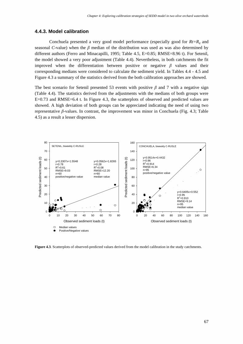
Chapter 4: Exploring calibration strategies of SEDD model in two olive orchard watersheds
67
4.4.3. Model calibration
Conchuela presented a very good model performance (especially good for Rt=Rq and
seasonal C-value) when the β median of the distribution was used as was also determined by
different authors (Ferro and Minacapilli, 1995; Table 4.5, E=0.85; RMSE=8.96 t). For Setenil,
the model showed a very poor adjustment (Table 4.4). Nevertheless, in both catchments the fit
improved when the differentiation between positive or negative β values and their
corresponding medians were considered to calculate the sediment yield. In Tables 4.4 - 4.5 and
Figure 4.3 a summary of the statistics derived from the both calibration approaches are showed.
The best scenario for Setenil presented 53 events with positive β and 7 with a negative sign
(Table 4.4). The statistics derived from the adjustments with the medians of both groups were
E=0.73 and RMSE=6.4 t. In Figure 4.3, the scatterplots of observed and predicted values are
showed. A high deviation of both groups can be appreciated indicating the need of using two
representative β-values. In contrast, the improvement was minor in Conchuela (Fig. 4.3; Table
4.5) as a result a lesser dispersion.
Figure 4.3. Scatterplots of observed-predicted values derived from the model calibration in the study catchments.
Observed sediment loads (t)
0 10 20 30 40 50 60 70 80
Pre
dic
ted s
edim
ent lo
ads (
t)
0
10
20
30
40
50
60
70
80
Median values
Positive/Negative values
y=0.3307x+1.5548r=0.78
R2=0.61
RMSE=9.03n=60positive/negative value
y=0.0562x+1.8265r=0.28
R2=0.08
RMSE=12.20n=60median value
SETENIL, biweekly C-RUSLE
Observed sediment loads (t)
0 20 40 60 80 100 120 140 160
Pre
dic
ted s
edim
ent lo
ads (
t)
0
20
40
60
80
100
120
140
160
y=0.9514x+0.4432r=0.96
R2=0.914
RMSE=6.34n=95positive/negative value
y=0.6405x+0.552r=0.95
R2=0.910
RMSE=9.14n=95median value
CONCHUELA, biweekly C-RUSLE
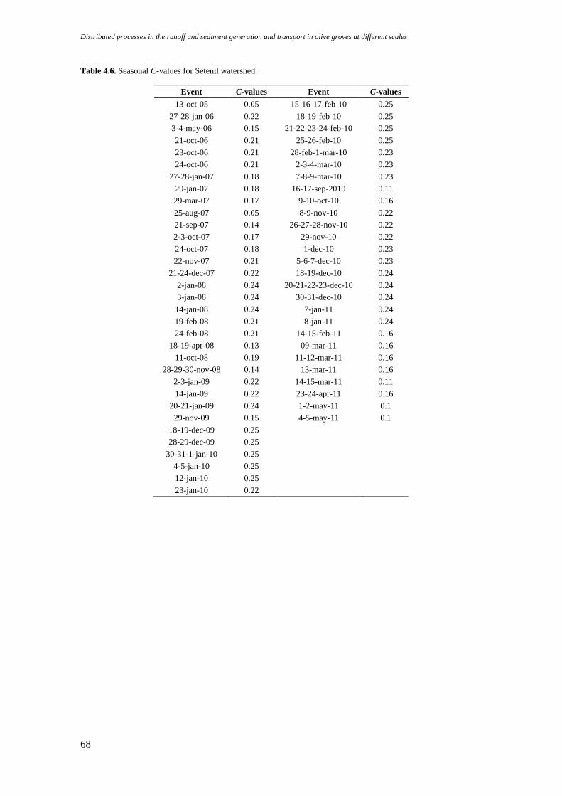
Distributed processes in the runoff and sediment generation and transport in olive groves at different scales
68
Table 4.6. Seasonal C-values for Setenil watershed.
Event C-values Event C-values
13-oct-05 0.05 15-16-17-feb-10 0.25
27-28-jan-06 0.22 18-19-feb-10 0.25
3-4-may-06 0.15 21-22-23-24-feb-10 0.25
21-oct-06 0.21 25-26-feb-10 0.25
23-oct-06 0.21 28-feb-1-mar-10 0.23
24-oct-06 0.21 2-3-4-mar-10 0.23
27-28-jan-07 0.18 7-8-9-mar-10 0.23
29-jan-07 0.18 16-17-sep-2010 0.11
29-mar-07 0.17 9-10-oct-10 0.16
25-aug-07 0.05 8-9-nov-10 0.22
21-sep-07 0.14 26-27-28-nov-10 0.22
2-3-oct-07 0.17 29-nov-10 0.22
24-oct-07 0.18 1-dec-10 0.23
22-nov-07 0.21 5-6-7-dec-10 0.23
21-24-dec-07 0.22 18-19-dec-10 0.24
2-jan-08 0.24 20-21-22-23-dec-10 0.24
3-jan-08 0.24 30-31-dec-10 0.24
14-jan-08 0.24 7-jan-11 0.24
19-feb-08 0.21 8-jan-11 0.24
24-feb-08 0.21 14-15-feb-11 0.16
18-19-apr-08 0.13 09-mar-11 0.16
11-oct-08 0.19 11-12-mar-11 0.16
28-29-30-nov-08 0.14 13-mar-11 0.16
2-3-jan-09 0.22 14-15-mar-11 0.11
14-jan-09 0.22 23-24-apr-11 0.16
20-21-jan-09 0.24 1-2-may-11 0.1
29-nov-09 0.15 4-5-may-11 0.1
18-19-dec-09 0.25
28-29-dec-09 0.25
30-31-1-jan-10 0.25
4-5-jan-10 0.25
12-jan-10 0.25
23-jan-10 0.22
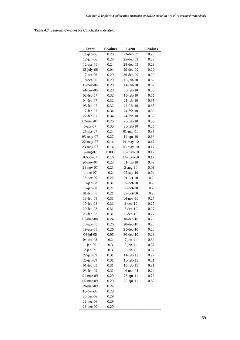
Chapter 4: Exploring calibration strategies of SEDD model in two olive orchard watersheds
69
Table 4.7. Seasonal C-values for Conchuela watershed.
Event C-values Event C-values
11-jan-06 0.28 23-dec-09 0.29
12-jan-06 0.28 25-dec-09 0.29
12-apr-06 0.24 28-dec-09 0.29
12-july-06 0.04 29-dec-09 0.29
17-oct-06 0.29 30-dec-09 0.29
18-oct-06 0.29 13-jan-10 0.32
15-nov-06 0.28 14-jan-10 0.32
24-nov-06 0.28 03-feb-10 0.33
02-feb-07 0.32 18-feb-10 0.35
04-feb-07 0.32 21-feb-10 0.35
05-feb-07 0.32 22-feb-10 0.35
17-feb-07 0.34 24-feb-10 0.35
22-feb-07 0.34 24-feb-10 0.35
02-mar-07 0.26 26-feb-10 0.35
5-apr-07 0.33 28-feb-10 0.35
25-apr-07 0.24 01-mar-10 0.35
05-may-07 0.27 14-apr-10 0.16
22-may-07 0.14 01-may-10 0.17
23-may-07 0.14 03-may-10 0.17
2-aug-07 0.009 13-may-10 0.17
02-oct-07 0.16 14-may-10 0.17
20-nov-07 0.23 01-jun-10 0.08
21-nov-07 0.23 3-aug-10 0.01
4-dec-07 0.2 05-sep-10 0.04
26-dec-07 0.22 01-oct-10 0.2
13-jan-08 0.31 02-oct-10 0.2
15-jan-08 0.27 05-oct-10 0.2
01-feb-08 0.21 29-oct-10 0.2
18-feb-08 0.31 14-nov-10 0.27
19-feb-08 0.31 1-dec-10 0.27
20-feb-08 0.31 2-dec-10 0.27
23-feb-08 0.31 5-dec-10 0.27
01-mar-08 0.24 18-dec-10 0.28
18-apr-08 0.26 20-dec-10 0.28
19-apr-08 0.26 21-dec-10 0.28
04-jul-08 0.05 30-dec-10 0.28
04-oct-08 0.2 7-jan-11 0.32
1-jan-09 0.3 8-jan-11 0.32
2-jan-09 0.3 9-jan-11 0.32
22-jan-09 0.31 14-feb-11 0.27
25-jan-09 0.31 16-feb-11 0.31
01-feb-09 0.31 19-feb-11 0.31
03-feb-09 0.31 14-mar-11 0.24
01-mar-09 0.29 23-apr-11 0.23
05-mar-09 0.29 29-apr-11 0.63
29-mar-09 0.24
18-dec-09 0.29
20-dec-09 0.29
22-dec-09 0.29
23-dec-09 0.29
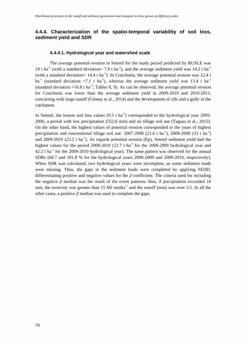
Distributed processes in the runoff and sediment generation and transport in olive groves at different scales
70
4.4.4. Characterization of the spatio-temporal variability of soil loss, sediment yield and SDR
4.4.4.1. Hydrological year and watershed scale
The average potential erosion in Setenil for the study period predicted by RUSLE was
19 t ha-1 (with a standard deviation= 7.9 t ha-1), and the average sediment yield was 14.2 t ha-1
(with a standard deviation= 14.4 t ha-1). In Conchuela, the average potential erosion was 12.4 t
ha-1 (standard deviation =7.1 t ha-1), whereas the average sediment yield was 13.4 t ha-1
(standard deviation =16.8 t ha-1; Tables 8, 9). As can be observed, the average potential erosion
for Conchuela was lower than the average sediment yield in 2009-2010 and 2010-2011,
concurring with large runoff (Gómez et al., 2014) and the development of rills and a gully in the
catchment.
In Setenil, the lowest soil loss values (9.5 t ha-1) corresponded to the hydrological year 2005-
2006, a period with low precipitation (552.6 mm) and no tillage soil use (Taguas et al., 2015).
On the other hand, the highest values of potential erosion corresponded to the years of highest
precipitation and conventional tillage soil use: 2007-2008 (21.6 t ha-1), 2008-2009 (33 t ha-1)
and 2009-2010 (23.2 t ha-1). As regards potential erosion (Ep), Setenil sediment yield had the
highest values for the period 2008-2010 (22.7 t ha-1 for the 2008-2009 hydrological year and
42.2 t ha-1 for the 2009-2010 hydrological year). The same pattern was observed for the annual
SDRs (68.7 and 181.8 % for the hydrological years 2008-2009 and 2009-2010, respectively).
When SDR was calculated, two hydrological years were incomplete, as some sediment loads
were missing. Thus, the gaps in the sediment loads were completed by applying SEDD,
differentiating positive and negative values for the β coefficient. The criteria used for including
the negative β median was the result of the event patterns: thus, if precipitation exceeded 10
mm, the erosivity was greater than 15 MJ mmha-1 and the runoff (mm) was over 3.5. In all the
other cases, a positive β median was used to complete the gaps.
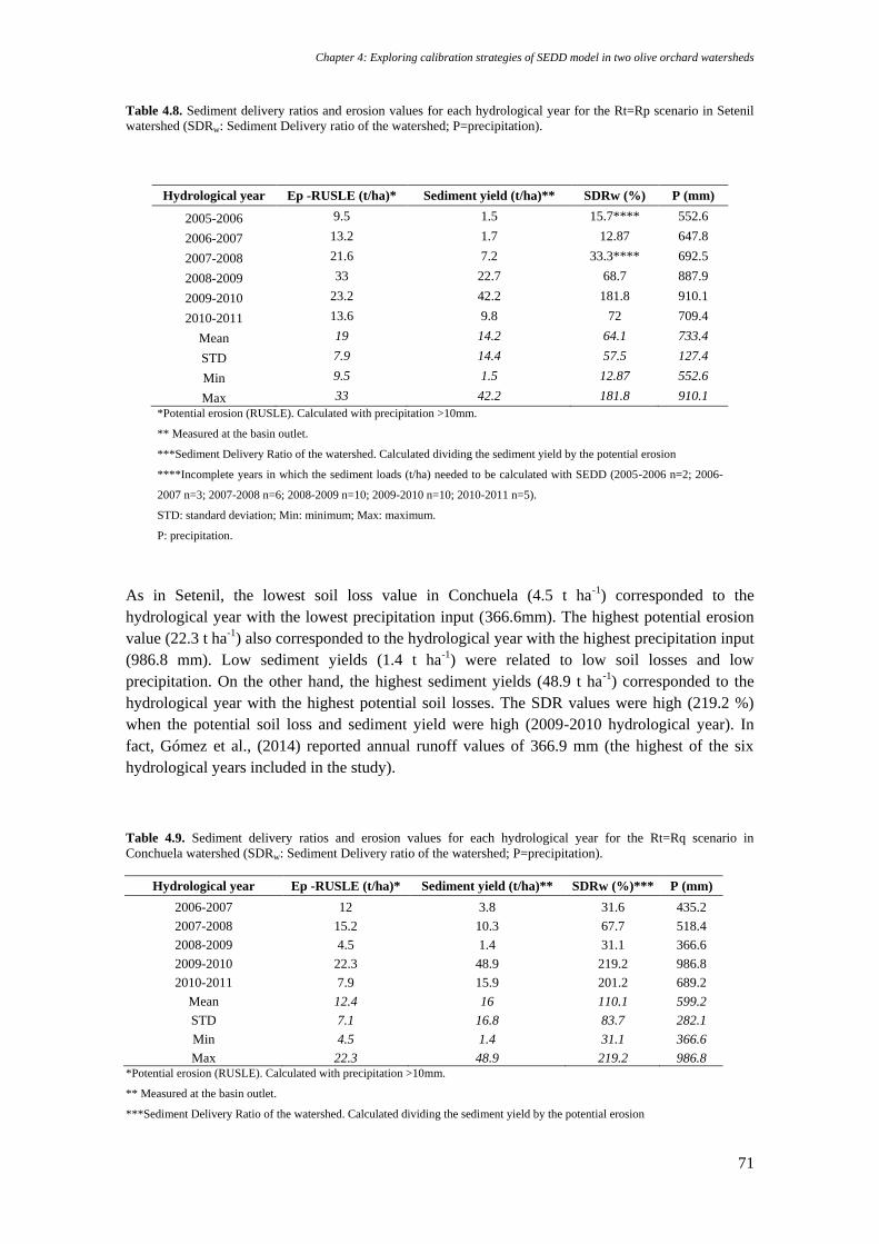
Chapter 4: Exploring calibration strategies of SEDD model in two olive orchard watersheds
71
Table 4.8. Sediment delivery ratios and erosion values for each hydrological year for the Rt=Rp scenario in Setenil
watershed (SDRw: Sediment Delivery ratio of the watershed; P=precipitation).
Hydrological year Ep -RUSLE (t/ha)* Sediment yield (t/ha)** SDRw (%) P (mm)
2005-2006 9.5 1.5 15.7**** 552.6
2006-2007 13.2 1.7 12.87 647.8
2007-2008 21.6 7.2 33.3**** 692.5
2008-2009 33 22.7 68.7 887.9
2009-2010 23.2 42.2 181.8 910.1
2010-2011 13.6 9.8 72 709.4
Mean 19 14.2 64.1 733.4
STD 7.9 14.4 57.5 127.4
Min 9.5 1.5 12.87 552.6
Max 33 42.2 181.8 910.1
*Potential erosion (RUSLE). Calculated with precipitation >10mm.
** Measured at the basin outlet.
***Sediment Delivery Ratio of the watershed. Calculated dividing the sediment yield by the potential erosion
****Incomplete years in which the sediment loads (t/ha) needed to be calculated with SEDD (2005-2006 n=2; 2006-
2007 n=3; 2007-2008 n=6; 2008-2009 n=10; 2009-2010 n=10; 2010-2011 n=5).
STD: standard deviation; Min: minimum; Max: maximum.
P: precipitation.
As in Setenil, the lowest soil loss value in Conchuela (4.5 t ha-1) corresponded to the
hydrological year with the lowest precipitation input (366.6mm). The highest potential erosion
value (22.3 t ha-1) also corresponded to the hydrological year with the highest precipitation input
(986.8 mm). Low sediment yields (1.4 t ha-1) were related to low soil losses and low
precipitation. On the other hand, the highest sediment yields (48.9 t ha-1) corresponded to the
hydrological year with the highest potential soil losses. The SDR values were high (219.2 %)
when the potential soil loss and sediment yield were high (2009-2010 hydrological year). In
fact, Gómez et al., (2014) reported annual runoff values of 366.9 mm (the highest of the six
hydrological years included in the study).
Table 4.9. Sediment delivery ratios and erosion values for each hydrological year for the Rt=Rq scenario in
Conchuela watershed (SDRw: Sediment Delivery ratio of the watershed; P=precipitation).
Hydrological year Ep -RUSLE (t/ha)* Sediment yield (t/ha)** SDRw (%)*** P (mm)
2006-2007 12 3.8 31.6 435.2
2007-2008 15.2 10.3 67.7 518.4
2008-2009 4.5 1.4 31.1 366.6
2009-2010 22.3 48.9 219.2 986.8
2010-2011 7.9 15.9 201.2 689.2
Mean 12.4 16 110.1 599.2
STD 7.1 16.8 83.7 282.1
Min 4.5 1.4 31.1 366.6
Max 22.3 48.9 219.2 986.8 *Potential erosion (RUSLE). Calculated with precipitation >10mm.
** Measured at the basin outlet.
***Sediment Delivery Ratio of the watershed. Calculated dividing the sediment yield by the potential erosion
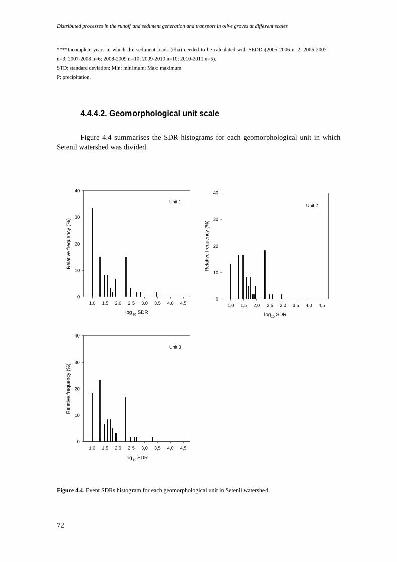
Distributed processes in the runoff and sediment generation and transport in olive groves at different scales
72
****Incomplete years in which the sediment loads (t/ha) needed to be calculated with SEDD (2005-2006 n=2; 2006-2007
n=3; 2007-2008 n=6; 2008-2009 n=10; 2009-2010 n=10; 2010-2011 n=5).
STD: standard deviation; Min: minimum; Max: maximum.
P: precipitation.
4.4.4.2. Geomorphological unit scale
Figure 4.4 summarises the SDR histograms for each geomorphological unit in which
Setenil watershed was divided.
Figure 4.4. Event SDRs histogram for each geomorphological unit in Setenil watershed.
log10
SDR
1,0 1,5 2,0 2,5 3,0 3,5 4,0 4,5
Re
lative
fre
qu
en
cy (
%)
0
10
20
30
40
Unit 1
log10
SDR
1,0 1,5 2,0 2,5 3,0 3,5 4,0 4,5
Re
lative
fre
qu
en
cy (
%)
0
10
20
30
40
Unit 2
log10
SDR
1,0 1,5 2,0 2,5 3,0 3,5 4,0 4,5
Rela
tive f
reque
ncy (
%)
0
10
20
30
40
Unit 3
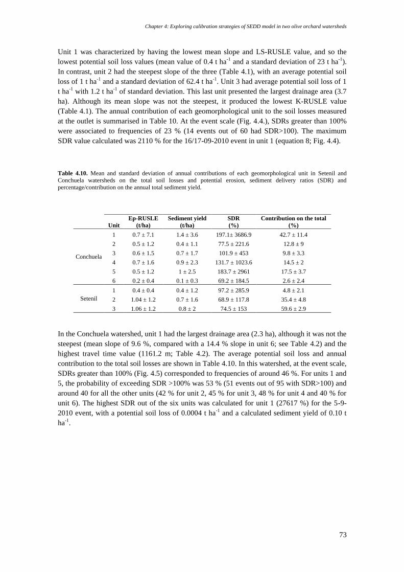
Chapter 4: Exploring calibration strategies of SEDD model in two olive orchard watersheds
73
Unit 1 was characterized by having the lowest mean slope and LS-RUSLE value, and so the
lowest potential soil loss values (mean value of 0.4 t ha-1 and a standard deviation of 23 t ha-1).
In contrast, unit 2 had the steepest slope of the three (Table 4.1), with an average potential soil
loss of 1 t ha-1 and a standard deviation of 62.4 t ha-1. Unit 3 had average potential soil loss of 1
t ha-1 with 1.2 t ha-1 of standard deviation. This last unit presented the largest drainage area (3.7
ha). Although its mean slope was not the steepest, it produced the lowest K-RUSLE value
(Table 4.1). The annual contribution of each geomorphological unit to the soil losses measured
at the outlet is summarised in Table 10. At the event scale (Fig. 4.4.), SDRs greater than 100%
were associated to frequencies of 23 % (14 events out of 60 had SDR>100). The maximum
SDR value calculated was 2110 % for the 16/17-09-2010 event in unit 1 (equation 8; Fig. 4.4).
Table 4.10. Mean and standard deviation of annual contributions of each geomorphological unit in Setenil and
Conchuela watersheds on the total soil losses and potential erosion, sediment delivery ratios (SDR) and
percentage/contribution on the annual total sediment yield.
Unit
Ep-RUSLE
(t/ha)
Sediment yield
(t/ha)
SDR
(%)
Contribution on the total
(%)
Conchuela
1 0.7 ± 7.1 1.4 ± 3.6 197.1± 3686.9 42.7 ± 11.4
2 0.5 ± 1.2 0.4 ± 1.1 77.5 ± 221.6 12.8 ± 9
3 0.6 ± 1.5 0.7 ± 1.7 101.9 ± 453 9.8 ± 3.3
4 0.7 ± 1.6 0.9 ± 2.3 131.7 ± 1023.6 14.5 ± 2
5 0.5 ± 1.2 1 ± 2.5 183.7 ± 2961 17.5 ± 3.7
6 0.2 ± 0.4 0.1 ± 0.3 69.2 ± 184.5 2.6 ± 2.4
Setenil
1 0.4 ± 0.4 0.4 ± 1.2 97.2 ± 285.9 4.8 ± 2.1
2 1.04 ± 1.2 0.7 ± 1.6 68.9 ± 117.8 35.4 ± 4.8
3 1.06 ± 1.2 0.8 ± 2 74.5 ± 153 59.6 ± 2.9
In the Conchuela watershed, unit 1 had the largest drainage area (2.3 ha), although it was not the
steepest (mean slope of 9.6 %, compared with a 14.4 % slope in unit 6; see Table 4.2) and the
highest travel time value (1161.2 m; Table 4.2). The average potential soil loss and annual
contribution to the total soil losses are shown in Table 4.10. In this watershed, at the event scale,
SDRs greater than 100% (Fig. 4.5) corresponded to frequencies of around 46 %. For units 1 and
5, the probability of exceeding SDR >100% was 53 % (51 events out of 95 with SDR>100) and
around 40 for all the other units (42 % for unit 2, 45 % for unit 3, 48 % for unit 4 and 40 % for
unit 6). The highest SDR out of the six units was calculated for unit 1 (27617 %) for the 5-9-
2010 event, with a potential soil loss of 0.0004 t ha-1 and a calculated sediment yield of 0.10 t
ha-1.

Distributed processes in the runoff and sediment generation and transport in olive groves at different scales
74
Figure 4.5. Event SDRs histogram for each geomorphological unit in Conchuela watershed.
log10
SDR
1,0 1,5 2,0 2,5 3,0 3,5 4,0 4,5
Re
lative
fre
qu
en
cy (
%)
0
10
20
30
40
Unit 1
log10
SDR
1,0 1,5 2,0 2,5 3,0 3,5 4,0 4,5
Re
lative
fre
qu
en
cy (
%)
0
10
20
30
40
Unit 2
log10
SDR
1,0 1,5 2,0 2,5 3,0 3,5 4,0 4,5
Rela
tive f
reque
ncy (
%)
0
10
20
30
40
Unit 4
log10
SDR
1,0 1,5 2,0 2,5 3,0 3,5 4,0 4,5
Rela
tive f
reque
ncy (
%)
0
10
20
30
40
Unit 5
log10
SDR
1,0 1,5 2,0 2,5 3,0 3,5 4,0 4,5
Rela
tive f
reque
ncy (
%)
0
10
20
30
40
Unit 6
log10
SDR
1,0 1,5 2,0 2,5 3,0 3,5 4,0 4,5
Rela
tive f
reque
ncy (
%)
0
10
20
30
40
Unit 3
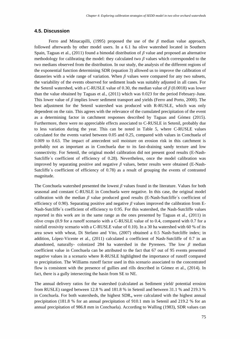
Chapter 4: Exploring calibration strategies of SEDD model in two olive orchard watersheds
75
4.5. Discussion
Ferro and Minacapilli, (1995) proposed the use of the β median value approach,
followed afterwards by other model users. In a 6.1 ha olive watershed located in Southern
Spain, Taguas et al., (2011) found a bimodal distribution of β value and proposed an alternative
methodology for calibrating the model: they calculated two β values which corresponded to the
two medians observed from the distribution. In our study, the analysis of the different regions of
the exponential function determining SDR (equation 3) allowed us to improve the calibration of
dataseries with a wide range of variation. When β values were compared for any two subsets,
the variability of the events observed for sediment loads was suitably adjusted in all cases. For
the Setenil watershed, with a C-RUSLE value of 0.30, the median value of β (0.0018) was lower
than the value obtained by Taguas et al., (2011) which was 0.023 for the period February-June.
This lower value of β implies lower sediment transport and yields (Ferro and Porto, 2000). The
best adjustment for the Setenil watershed was produced with R-RUSLE, which was only
dependent on the rain. This agrees with the relevance of the cumulated precipitation of the event
as a determining factor in catchment responses described by Taguas and Gómez (2015).
Furthermore, there were no appreciable effects associated to C-RUSLE in Setenil, probably due
to less variation during the year. This can be noted in Table 5, where C-RUSLE values
calculated for the events varied between 0.05 and 0.25, compared with values in Conchuela of
0.009 to 0.63. The impact of antecedent soil moisture on erosion risk in this catchment is
probably not as important as in Conchuela due to its fast-draining sandy texture and low
connectivity. For Setenil, the original model calibration did not present good results (E-Nash-
Sutcliffe´s coefficient of efficiency of 0.28). Nevertheless, once the model calibration was
improved by separating positive and negative β values, better results were obtained (E-Nash-
Sutcliffe´s coefficient of efficiency of 0.78) as a result of grouping the events of contrasted
magnitude.
The Conchuela watershed presented the lowest β values found in the literature. Values for both
seasonal and constant C-RUSLE in Conchuela were negative. In this case, the original model
calibration with the median β value produced good results (E-Nash-Sutcliffe´s coefficient of
efficiency of 0.90). Separating positive and negative β values improved the calibration from E-
Nash-Sutcliffe´s coefficient of efficiency to 0.95. For this watershed, the Nash-Sutcliffe values
reported in this work are in the same range as the ones presented by Taguas et al., (2011) in
olive crops (0.9 for a runoff scenario with a C-RUSLE value of to 0.4, compared with 0.7 for a
rainfall erosivity scenario with a C-RUSLE value of 0.10). In a 30 ha watershed with 60 % of its
area sown with wheat, Di Stefano and Vito, (2007) obtained a 0.5 Nash-Sutcliffe index; in
addition, López-Vicente et al., (2011) calculated a coefficient of Nash-Sutcliffe of 0.7 in an
abandoned, naturally- colonized 284 ha watershed in the Pyrenees. The low β median
coefficient value in Conchuela can be attributed to the fact that 67 out of 95 events presented
negative values in a scenario where R-RUSLE highlighted the importance of runoff compared
to precipitation. The Williams runoff factor used in this scenario associated to the concentrated
flow is consistent with the presence of gullies and rills described in Gómez et al., (2014). In
fact, there is a gully intersecting the basin from SE to NE.
The annual delivery ratios for the watershed (calculated as Sediment yield/ potential erosion
from RUSLE) ranged between 12.8 % and 181.8 % in Setenil and between 31.1 % and 219.3 %
in Conchuela. For both watersheds, the highest SDRw were calculated with the highest annual
precipitation (181.8 % for an annual precipitation of 910.1 mm in Setenil and 219.2 % for an
annual precipitation of 986.8 mm in Conchuela). According to Walling (1983), SDR values can
Distributed processes in the runoff and sediment generation and transport in olive groves at different scales
76
vary from 0.1 to 100% at the annual scale, as the equations to calculate it were developed for
basins from particular regions. Values close to 100 % are also reported in the work of Fernández
et al., (2003), Fu et al., (2006) and López-Vicente et al., (2011). These high SDRw are explained
by what Walling (1983) describes as a 'temporal paradox'. This paradox is defined as the
temporal attenuation due to sediment storage and remobilisation within the watershed, no matter
the size. This idea was supported by the work of Priest et al., (1975) who reported SDRw
between 1 % and 554 % at the event scale in the Treynor watershed (U.S), or Duijsings, (1986)
who reported seasonal (winter vs. summer) SDR of nearly 100% in a Luxembourg basin.
Walling (1983) interpreted these high values as showing that sediment from past events stored
into the channel network or deposited on the hillslopes can be removed, thus increasing the
amount of available sediment for its transport to the basin outlet. In fact, Ferro and Porto (2000)
stated that SDRw can be above 100%, meaning that the sediment stored in the channel network
or deposited on the hillslopes in previous events can be removed. In the case of Setenil and
Conchuela, high SDRw values were attributed to sediment sources that are not computed by the
RUSLE equation when calculating potential erosion at the hillslope scale. The SEDD model
was devised for small catchments and did not consider channel processes (Ferro and Porto,
2000). However, in Conchuela, gully processes necessarily play a major role. In fact, Gómez et
al., (2014) highlighted the significant role of rills and gullies as well as peak flow (Rt=Rq) in
sediment transport in the catchment, and the fact that in relation to rill and gullies it constitutes
the main type of erosion in the watershed. In the Setenil watershed, although there is an
ephemeral gully (width >30 cm) and a small gully in unit 3, the main sediment sources are
associated with sheetwash and rills. Our interpretation of the SDR value of > 100% in both olive
catchments is that this is the model’s numerical answer to the problem of incorporating
sediment losses that can only be due to activation of gully erosion processes and/or channel
contribution, which also includes remobilization of sediment deposited within the catchment
from previous storms. This behaviour of the model also explains a large fraction of the negative
β vales.
A variable C-RUSLE factor is a more consistent parameter than the annual C-RUSLE value
adapted to the management and other factors such as soil moisture. It should be calculated,
among other reasons, when the impact of the management is significant and/or wide variations
in soil moisture are expected. This might be a major factor with vertisols, such as in the case of
Conchuela. Gómez et al., (2003), in a model analysis of an olive orchard in Southern Spain,
calculated different C-RUSLE values depending on different conservation strategies (from non-
tillage to full cover crop). Each soil management technique had its own C-RUSLE, thus
showing the importance of the calculation of this RUSLE value. In the literature, the most
widely extended use of C-RUSLE in SEDD calibration is a unique value, possibly because most
studies were not carried out on agricultural areas or because of the great complexity on a larger
spatial scale. For instance, Jain and Kothyari (2000) attributed a unique C-RUSLE value based
on land cover categories estimated using Landsat TM and IRS 1C LISS-III data; Fernández et
al., (2003) used a unique value for rangelands and forests from the literature; Di Stefano et al.,
(2005) set a value of 0.164 for an ungauged basin; Fu et al., (2006) calculated the C-RUSLE
value following RUSLE and use one value for crop rotation and another for land use practice.
However, although they did not calculate the seasonal value, some authors used a C-RUSLE
value which was more consistent with the watershed crop or land use. For example, Di Stefano
and Ferro (2007) divided the basin into areas with the same crop and, for each polygon into
which the basin was divided, a C-RUSLE value was assigned (wheat=0.45, olive trees=0.41,
urbanized areas=1, bare fallow soil =1). In addition, Taguas et al., (2011) tried different values
Chapter 4: Exploring calibration strategies of SEDD model in two olive orchard watersheds
77
of C-RUSLE measured in olive crops (from 0.01 to 0.5) and kept the one that gave the best
results (0.4 and 0.1 for runoff and precipitation scenarios, respectively). The predicted soil loss
values for both watersheds were in the same range as the ones predicted by Taguas et al., (2011)
in olive orchards in Southern Spain or the ones predicted in a U.S. cropland watershed by
Fernández et al., (2003).
At the geomorphological unit and event scale, the most efficient unit at exporting sediments in
Setenil was unit 1, with a mean unit SDR of 100 % (standard deviation 285.9 %) whereas the
lowest (67.3 %, standard deviation 117.80 %) was observed in unit 2. Nevertheless, unit 1 had
the lowest potential erosion values (0.4 t ha-1). At the watershed scale, the SDRw mean value
was 64.1 % (standard deviation 57.5 %). This is linked to the longest travel time, thus indicating
high probability that the eroded particles arrive from the source to the nearest stream (Ferro and
Minacapilli, 1995). In both cases, the observed variation ranges of event SDRs were notably
narrower than the ones described by Taguas et al., (2011) in an olive orchard catchment with an
annual precipitation of 400 mm and more arid features. In the case of the Conchuela watershed,
the most efficient units at exporting sediments were units 1 (mean SDR of 200 % and a standard
deviation of 3686.9 %, concurring with the biggest areas) and 5 (mean SDR 200 % and standard
deviation 2961 %). On the other hand, the least efficient unit was unit 6 (mean SDR value 50 %
and standard deviation 184.53 %). At the catchment scale, the average SDR value was 94.2 %,
with a standard deviation of 83.7 %. Unlike the Setenil watershed, in the Conchuela watershed,
the unit with the highest potential soil losses and contribution to the sediment measured at the
outlet was also unit 1.
Annual SDRs in both watersheds indicated very active dynamical sediment transport. Extreme
SDR values (>100%) were associated with very humid years with precipitation values at least
30 % higher than the annual average. At the event scale, similar tendencies were observed and
SDRs >100% were linked to frequencies of 23 % in Setenil and 53 % in Conchuela, which
might mean that for these fractions of events, total loads in the outlet would transport sediment
detached in previous events.
In terms of soil conservation practices such as mulching or the use of cover crops between the
lanes, the greatest efforts should be made in unit 3 in the Setenil watershed, as it contributed
59.7 % of the total sediment measured at the basin outlet and also had the highest sediment
yield (0.8 t ha-1). In the case of the Conchuela watershed, these efforts should be made in unit 1,
which contributed 42.7 % of the total sediment measured at the basin outlet and, as in Setenil,
had the highest sediment yield (1.43 t ha-1). In order to control gullies in these agricultural areas,
check dams were installed in 2012.
4.6. Conclusions
The SEDD model was successfully calibrated in the Conchuela watershed, while poor
adjustments were found for the Setenil watershed. In this calibration, different R-RUSLE
values, indicating different watershed hydrological responses, were observed. For instance, in
Conchuela the best calibration scenarios were associated with concentrated flow-dependent
erosivities or runoff values. On the other hand, the erosivity value for the Setenil watershed was
only rain-dependent. Eventually, seasonal C-RUSLE values should be included when there are
major changes in the impact of soil management due to soil humidity, as in the case of the
Conchuela watershed with a vertic soil.
Distributed processes in the runoff and sediment generation and transport in olive groves at different scales
78
The analysis of the different calibration strategies allowed us to improve the adjustment in the
Setenil watershed. To do so, the events were separated into positive or negative values
according to the sign of the β parameter. The medians of these groups of events allowed us to
obtain an E value of 0.7 and an RMSE of 6.4. In the Conchuela watershed, only minor
improvements to this variation in the model calibration were possible (E value of 0.9 and an
RMSE of 6.3).
The annual SDR values indicated a very active dynamic in both watersheds. The mean annual
SDR in the Setenil watershed was 64 %, with a range of variation for a six-year period between
181.8 and 12.8 %. In Conchuela, it was 94 % (ranging between 219.2 and 14.2 %). Extreme
SDR values were associated to very humid years with precipitation values around 30 % higher
than the annual average. At the event scale, it was possible to isolate the most active areas in
terms of sediment contribution to the watershed outlet and improve the soil conservation
measures in these areas.
Acknowledgements
The author would like to thank Nieves Marimón for her invaluable help and support.
This study was supported by Project P08-AGR-03925 (Andalusian Government), AGL2009-
12936-C03-01 (Ministry of Science and Innovation), RESEL (Ministry of Agriculture, Food
and Environment) and FEDER funds. We would also like to thank the JAE program of the
National Spanish Research Centre, which provided grant support for the corresponding author’s
PhD project. We are also very grateful to Francisco Natera and Alonso Zamudio, owners of the
study farms.

General Conclusions
79
Chapter 5
General Conclusions
‘This is the end, beautiful friend
This is the end, my only friend, the end
Of our elaborate plans, the end
Of everything that stands, the end
No safety or surprise, the end’.
Jim Morrison. The End. The Doors (1967)

Distributed processes in the runoff and sediment generation and transport in olive groves at different scales
80
General Conclusions
81
5.1. General Conclusions
This study highlights the need of considering upscaling measures from on-off to the
watershed scale in olive orchards under semi-arid Mediterranean environments in order to have
the best soil conservation measures implementation and thus, reduce soil erosion and sediment
deposition. A combination of both field measures and sediment delivery physical modelling was
used to throw light to the described effects.
1. The one-off scale Soil Water Repellency (SWR) measurements in olive orchards
showed that it occurs at a low or moderate intensity (average values of 49 s, considered
slightly wettable). SWR presents a high spatial variability with hydrophobic areas
nearby to non-hydrophobic areas which could infiltrate the excess of water trough
runoff processes. This indicates that the hydrological relevance of the process in
commercial olive farms at hillslope and catchment scale will be very small or even it
might be negligible. Wettable SWR began to appear in summer under the tree canopy
(except for the conventional tillage orchard), got the highest values in the lanes between
trees in autumn (especially in the cover crop orchard) and disappeared in winter.
However, when appeared (even in a moderate intensity) it tended to be concentrated in
the area under the olive tree canopy, where the concentration of organic carbon content
and soil moisture was higher. In fact, for summer and autumn measurements, a
correlation between organic matter content and soil water repellency was found (r2=
0.92).
2. At the hillslope runoff-plot scale, the use of vegetation cover strips combined with
magnetic iron oxides and simulated rainfall, allowed to identify distribution patterns of
sediment redistribution for different management operations. Vegetation strips caused
selective fine texture particle size transports which come from the closest area to the
plot outlet. Tillage resulted very effective to diminish runoff and soil losses (50 % and
12% respectively lower if compared to bare soil) and increasing infiltration when it is
recently performed, a situation that changes when it gets consolidated and degraded. It
is with this last situation when high soil erosion rates (soil losses up to 15 kg) and
sediment transport interconnection along the slope occurs. Vegetation cover strips under
Mediterranean conditions, should be then a safeguarding in order to maintain the
discontinuity in moment with high runoff responses.
3. At the watershed scale, the use of SEDD model allowed the identification of the areas more
prone to erosion in two olive crop watersheds of very different environmental characteristics.
Different calibration alternatives based on the analysis of R-RUSLE, C- RUSLE and β, (an
empirical parameter which controls the travel time in the different geomorphological areas in the
catchment) were explored. A new calibration strategy based on the adjustment of the dataseries
range to the regions of the exponential function that determine the SEDD was proposed. Thus,
we proposed by separating β-positive or β-negative values to adjust sediment loads of events
when outliers were found such as the case of Setenil. The results allowed the evaluation of the
areas to concentrate the control measures through the analyses of the values of sediment delivery
ratios. The extrapolation of the use of SEDD to other catchments with different attributes is not
advisable without a previous calibration.
Distributed processes in the runoff and sediment generation and transport in olive groves at different scales
82
5.2. Future Research Lines
This thesis shows the importance of considering different scale measurements when
studying sediment transport processes in order to have the best soil conservation strategies
implementation. From the above findings and limitations, the following research lines are now
open.
Soil water repellency
- Despite this work has shown that the SWR influence in the runoff generation and thus, in soil losses,
is small, it is a process which can be found under the tree canopy. This area is known to have
relatively high organic matter content, facilitating the appearance of hydrophobic spots. In order to
have a complete study of the appearance of SWR in olive crops, two research lines can be open. [i]
soil humidity measured with sensors through an entire olive watershed could be correlated with
SWR measurements. For this, SWR could be measured with the WDPT test in those areas where the
sensors are placed. At the same time, a profile distribution of the soil humidity and SWR could be
measured with the sensor data and the field WDPT measurements. [2] On the other hand, as organic
matter appears to have significant influence in the SWR appearance, a chemical analysis of the type
of organic matter found under the canopies and on the tree rows could be done. Both research lines
would be performed for, at least, two hydrological years and in two orchards with the same soil
management system (as it has been shown that the tillage systems only affects SWR when it is
related to cover crops).
Vegetation trapping efficiency
- Once studied and determined the efficiency of the vegetation strips for trapping sediments at the plot
scale, the next step would be to quantify the total amount of sediment trapped by the strips and of
which particle size. To do so, and at a larger scale, the same experiment can be replicate in an
experimental olive watershed. Several vegetation strips could be implemented and the rows between
trees could be tagged with magnetic iron oxide. With this, it would be easy to determine the
influence of soil management in the sediment transport.
Sediment Delivery Ratio (SDR)
- SEDD model allowed the identification of the geomorphological areas within a catchment more
prone to soil erosion and thus, more efficient in sediment transport. Within this frame, the
identification of carbon sources and sinks is of interest. The isotopic signature of δ13C is one the
techniques that could allow estimating those sources and sinks. This work started in 2012 with Dr
Richard Brazier (University of Exeter) and the main hypothesis to be tested are: [1] are there any
differences/ relationships between C3 and C4 along the catchment?; [2] Are there any
differences/similarities in δ13C between the soil collected in the outlet and the soil collected in the
hillslope plots?; [3] is there any relationship between total organic carbon (TOC) and δ13C?; [4]
Can we prove that vegetation cover has influence in retaining soil, so soil conservation practices can
be improved? Finding the sources and sinks of the in the catchment (lanes or under the tree canopy
as well as different soil profile depths), would allow me to discriminate if the vegetation is really
helping to prevent soil loss (and if so, give it a number). This might be strongly correlated to the
results found in the SOC distribution. In the case that the isotopic signature is not different,
vegetation η-alkanes values would be used for the atomic discrimination.

Appendixes
83
APPENDIX 1
Hydrological attributes of the observed events for the study period in Setenil
watershed

Distributed processes in the runoff and sediment generation and transport in olive groves at different scales
84
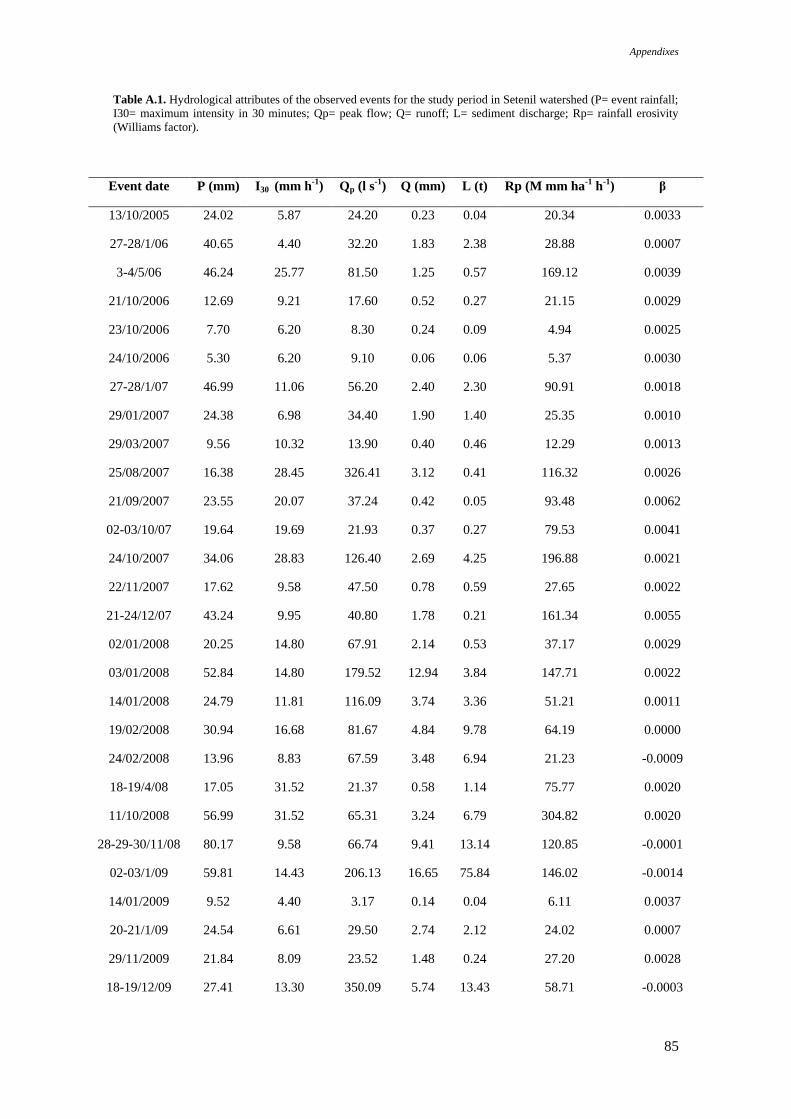
Appendixes
85
Table A.1. Hydrological attributes of the observed events for the study period in Setenil watershed (P= event rainfall;
I30= maximum intensity in 30 minutes; Qp= peak flow; Q= runoff; L= sediment discharge; Rp= rainfall erosivity
(Williams factor).
Event date P (mm) I30 (mm h-1
) Qp (l s-1
) Q (mm) L (t) Rp (M mm ha-1
h-1
) β
13/10/2005 24.02 5.87 24.20 0.23 0.04 20.34 0.0033
27-28/1/06 40.65 4.40 32.20 1.83 2.38 28.88 0.0007
3-4/5/06 46.24 25.77 81.50 1.25 0.57 169.12 0.0039
21/10/2006 12.69 9.21 17.60 0.52 0.27 21.15 0.0029
23/10/2006 7.70 6.20 8.30 0.24 0.09 4.94 0.0025
24/10/2006 5.30 6.20 9.10 0.06 0.06 5.37 0.0030
27-28/1/07 46.99 11.06 56.20 2.40 2.30 90.91 0.0018
29/01/2007 24.38 6.98 34.40 1.90 1.40 25.35 0.0010
29/03/2007 9.56 10.32 13.90 0.40 0.46 12.29 0.0013
25/08/2007 16.38 28.45 326.41 3.12 0.41 116.32 0.0026
21/09/2007 23.55 20.07 37.24 0.42 0.05 93.48 0.0062
02-03/10/07 19.64 19.69 21.93 0.37 0.27 79.53 0.0041
24/10/2007 34.06 28.83 126.40 2.69 4.25 196.88 0.0021
22/11/2007 17.62 9.58 47.50 0.78 0.59 27.65 0.0022
21-24/12/07 43.24 9.95 40.80 1.78 0.21 161.34 0.0055
02/01/2008 20.25 14.80 67.91 2.14 0.53 37.17 0.0029
03/01/2008 52.84 14.80 179.52 12.94 3.84 147.71 0.0022
14/01/2008 24.79 11.81 116.09 3.74 3.36 51.21 0.0011
19/02/2008 30.94 16.68 81.67 4.84 9.78 64.19 0.0000
24/02/2008 13.96 8.83 67.59 3.48 6.94 21.23 -0.0009
18-19/4/08 17.05 31.52 21.37 0.58 1.14 75.77 0.0020
11/10/2008 56.99 31.52 65.31 3.24 6.79 304.82 0.0020
28-29-30/11/08 80.17 9.58 66.74 9.41 13.14 120.85 -0.0001
02-03/1/09 59.81 14.43 206.13 16.65 75.84 146.02 -0.0014
14/01/2009 9.52 4.40 3.17 0.14 0.04 6.11 0.0037
20-21/1/09 24.54 6.61 29.50 2.74 2.12 24.02 0.0007
29/11/2009 21.84 8.09 23.52 1.48 0.24 27.20 0.0028
18-19/12/09 27.41 13.30 350.09 5.74 13.43 58.71 -0.0003
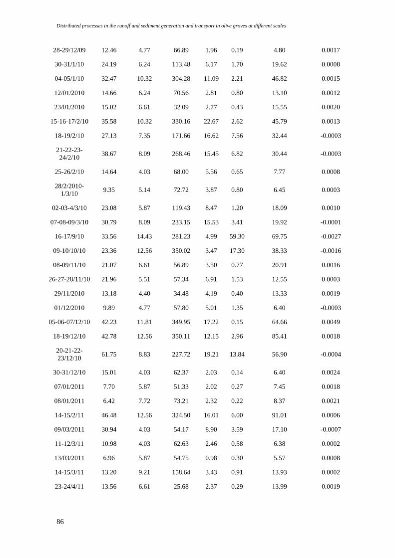
Distributed processes in the runoff and sediment generation and transport in olive groves at different scales
86
28-29/12/09 12.46 4.77 66.89 1.96 0.19 4.80 0.0017
30-31/1/10 24.19 6.24 113.48 6.17 1.70 19.62 0.0008
04-05/1/10 32.47 10.32 304.28 11.09 2.21 46.82 0.0015
12/01/2010 14.66 6.24 70.56 2.81 0.80 13.10 0.0012
23/01/2010 15.02 6.61 32.09 2.77 0.43 15.55 0.0020
15-16-17/2/10 35.58 10.32 330.16 22.67 2.62 45.79 0.0013
18-19/2/10 27.13 7.35 171.66 16.62 7.56 32.44 -0.0003
21-22-23-
24/2/10 38.67 8.09 268.46 15.45 6.82 30.44 -0.0003
25-26/2/10 14.64 4.03 68.00 5.56 0.65 7.77 0.0008
28/2/2010-
1/3/10 9.35 5.14 72.72 3.87 0.80 6.45 0.0003
02-03-4/3/10 23.08 5.87 119.43 8.47 1.20 18.09 0.0010
07-08-09/3/10 30.79 8.09 233.15 15.53 3.41 19.92 -0.0001
16-17/9/10 33.56 14.43 281.23 4.99 59.30 69.75 -0.0027
09-10/10/10 23.36 12.56 350.02 3.47 17.30 38.33 -0.0016
08-09/11/10 21.07 6.61 56.89 3.50 0.77 20.91 0.0016
26-27-28/11/10 21.96 5.51 57.34 6.91 1.53 12.55 0.0003
29/11/2010 13.18 4.40 34.48 4.19 0.40 13.33 0.0019
01/12/2010 9.89 4.77 57.80 5.01 1.35 6.40 -0.0003
05-06-07/12/10 42.23 11.81 349.95 17.22 0.15 64.66 0.0049
18-19/12/10 42.78 12.56 350.11 12.15 2.96 85.41 0.0018
20-21-22-
23/12/10 61.75 8.83 227.72 19.21 13.84 56.90 -0.0004
30-31/12/10 15.01 4.03 62.37 2.03 0.14 6.40 0.0024
07/01/2011 7.70 5.87 51.33 2.02 0.27 7.45 0.0018
08/01/2011 6.42 7.72 73.21 2.32 0.22 8.37 0.0021
14-15/2/11 46.48 12.56 324.50 16.01 6.00 91.01 0.0006
09/03/2011 30.94 4.03 54.17 8.90 3.59 17.10 -0.0007
11-12/3/11 10.98 4.03 62.63 2.46 0.58 6.38 0.0002
13/03/2011 6.96 5.87 54.75 0.98 0.30 5.57 0.0008
14-15/3/11 13.20 9.21 158.64 3.43 0.91 13.93 0.0002
23-24/4/11 13.56 6.61 25.68 2.37 0.29 13.99 0.0019

Appendixes
87
01-2/5/11 20.58 8.83 119.44 6.47 0.80 35.03 0.0013
04-5/5/11 13.8 10.69 283.74 6.73 2.93 25.98 -0.0005
Mean 25.76 10.55 117.39 5.47 4.88 49.98 0.0014
STD 15.85 6.84 110.03 5.62 12.45 57.39 0.0017
Min 5.30 4.03 3.17 0.06 0.04 4.80 -0.0027
Max 80.17 31.52 350.11 22.67 75.84 304.82 0.0062
Median 22.52 8.83 67.24 3.335 1.03 26.59 0.0013

Distributed processes in the runoff and sediment generation and transport in olive groves at different scales
88

Appendixes
89
APPENDIX 2
Hydrological attributes of the observed events for the study period in Conchuela
watershed

Distributed processes in the runoff and sediment generation and transport in olive groves at different scales
90
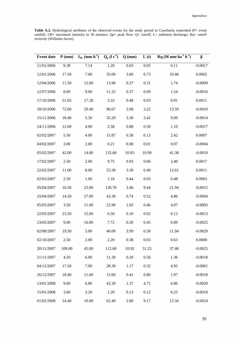
Appendixes
91
Table A.2. Hydrological attributes of the observed events for the study period in Conchuela watershed (P= event
rainfall; I30= maximum intensity in 30 minutes; Qp= peak flow; Q= runoff; L= sediment discharge; Rq= runoff
erosivity (Williams factor).
Event date P (mm) I30 (mm h-1
) Qp (l s-1
) Q (mm) L (t) Rq (M mm ha-1
h-1
) β
11/01/2006 9.38 7.14 1.20 0.03 0.05 0.11 -0.0017
12/01/2006 17.50 7.00 35.00 3.60 0.73 10.46 0.0002
12/04/2006 11.50 12.00 13.90 0.37 0.31 1.74 -0.0009
12/07/2006 8.00 9.00 11.25 0.37 0.09 1.54 -0.0016
17/10/2006 51.05 17.28 3.33 0.48 0.03 0.91 0.0011
18/10/2006 72.60 29.40 96.67 2.08 3.22 13.59 -0.0010
15/11/2006 18.40 5.30 35.20 3.30 3.42 9.99 -0.0014
24/11/2006 12.00 4.00 2.58 0.88 0.50 1.10 -0.0017
02/02/2007 5.50 4.00 15.87 0.58 0.13 2.42 0.0007
04/02/2007 3.00 2.00 0.21 0.08 0.01 0.07 -0.0004
05/02/2007 42.00 14.00 135.60 10.83 10.99 41.38 -0.0010
17/02/2007 2.50 2.00 9.75 0.93 0.06 2.40 0.0017
22/02/2007 11.00 8.00 53.30 3.30 0.49 12.61 0.0011
02/03/2007 2.50 1.00 1.18 0.44 0.03 0.48 0.0003
05/04/2007 16.50 23.00 136.70 3.46 9.44 21.94 -0.0015
25/04/2007 14.50 27.00 43.30 0.74 0.52 4.86 -0.0004
05/05/2007 3.50 11.00 22.90 1.02 0.46 4.07 -0.0003
22/05/2007 23.50 15.00 0.50 0.10 0.02 0.13 -0.0013
23/05/2007 9.00 16.00 7.72 0.20 0.45 0.89 -0.0025
02/08/2007 19.50 5.00 40.00 3.99 0.58 11.94 -0.0029
02/10/2007 2.50 2.00 2.20 0.38 0.03 0.63 0.0000
20/11/2007 109.00 45.00 112.60 10.92 31.25 37.46 -0.0025
21/11/2007 4.50 6.00 11.30 0.29 0.56 1.36 -0.0018
04/12/2007 17.50 7.00 28.30 1.17 0.32 4.95 -0.0001
26/12/2007 18.40 11.60 15.60 0.41 0.80 1.97 -0.0018
13/01/2008 9.00 6.80 43.30 1.37 4.71 6.86 -0.0020
15/01/2008 3.60 3.20 1.20 0.13 0.12 0.25 -0.0018
01/02/2008 24.40 10.00 62.40 2.80 9.17 12.56 -0.0024
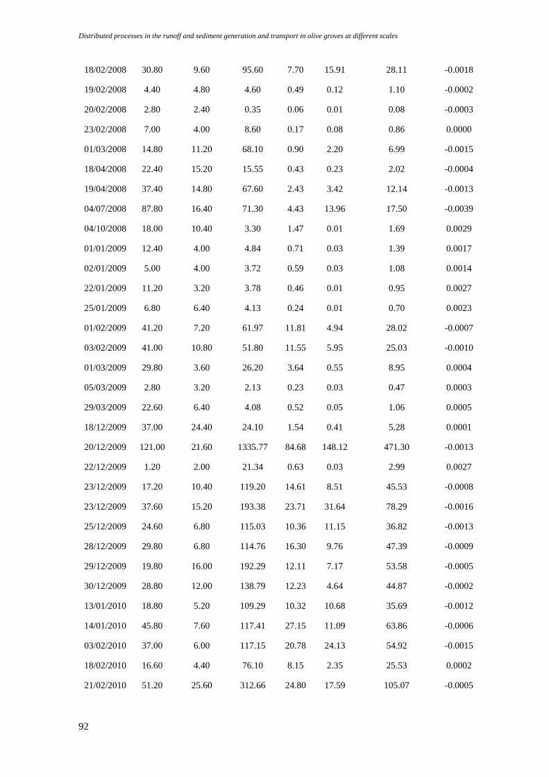
Distributed processes in the runoff and sediment generation and transport in olive groves at different scales
92
18/02/2008 30.80 9.60 95.60 7.70 15.91 28.11 -0.0018
19/02/2008 4.40 4.80 4.60 0.49 0.12 1.10 -0.0002
20/02/2008 2.80 2.40 0.35 0.06 0.01 0.08 -0.0003
23/02/2008 7.00 4.00 8.60 0.17 0.08 0.86 0.0000
01/03/2008 14.80 11.20 68.10 0.90 2.20 6.99 -0.0015
18/04/2008 22.40 15.20 15.55 0.43 0.23 2.02 -0.0004
19/04/2008 37.40 14.80 67.60 2.43 3.42 12.14 -0.0013
04/07/2008 87.80 16.40 71.30 4.43 13.96 17.50 -0.0039
04/10/2008 18.00 10.40 3.30 1.47 0.01 1.69 0.0029
01/01/2009 12.40 4.00 4.84 0.71 0.03 1.39 0.0017
02/01/2009 5.00 4.00 3.72 0.59 0.03 1.08 0.0014
22/01/2009 11.20 3.20 3.78 0.46 0.01 0.95 0.0027
25/01/2009 6.80 6.40 4.13 0.24 0.01 0.70 0.0023
01/02/2009 41.20 7.20 61.97 11.81 4.94 28.02 -0.0007
03/02/2009 41.00 10.80 51.80 11.55 5.95 25.03 -0.0010
01/03/2009 29.80 3.60 26.20 3.64 0.55 8.95 0.0004
05/03/2009 2.80 3.20 2.13 0.23 0.03 0.47 0.0003
29/03/2009 22.60 6.40 4.08 0.52 0.05 1.06 0.0005
18/12/2009 37.00 24.40 24.10 1.54 0.41 5.28 0.0001
20/12/2009 121.00 21.60 1335.77 84.68 148.12 471.30 -0.0013
22/12/2009 1.20 2.00 21.34 0.63 0.03 2.99 0.0027
23/12/2009 17.20 10.40 119.20 14.61 8.51 45.53 -0.0008
23/12/2009 37.60 15.20 193.38 23.71 31.64 78.29 -0.0016
25/12/2009 24.60 6.80 115.03 10.36 11.15 36.82 -0.0013
28/12/2009 29.80 6.80 114.76 16.30 9.76 47.39 -0.0009
29/12/2009 19.80 16.00 192.29 12.11 7.17 53.58 -0.0005
30/12/2009 28.80 12.00 138.79 12.23 4.64 44.87 -0.0002
13/01/2010 18.80 5.20 109.29 10.32 10.68 35.69 -0.0012
14/01/2010 45.80 7.60 117.41 27.15 11.09 63.86 -0.0006
03/02/2010 37.00 6.00 117.15 20.78 24.13 54.92 -0.0015
18/02/2010 16.60 4.40 76.10 8.15 2.35 25.53 0.0002
21/02/2010 51.20 25.60 312.66 24.80 17.59 105.07 -0.0005
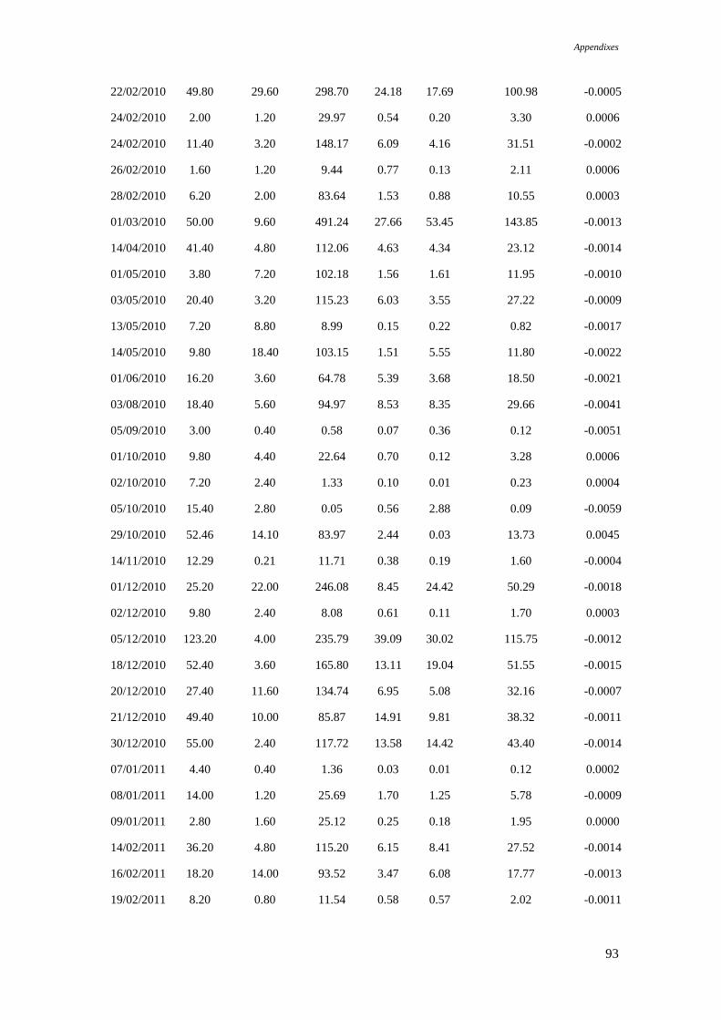
Appendixes
93
22/02/2010 49.80 29.60 298.70 24.18 17.69 100.98 -0.0005
24/02/2010 2.00 1.20 29.97 0.54 0.20 3.30 0.0006
24/02/2010 11.40 3.20 148.17 6.09 4.16 31.51 -0.0002
26/02/2010 1.60 1.20 9.44 0.77 0.13 2.11 0.0006
28/02/2010 6.20 2.00 83.64 1.53 0.88 10.55 0.0003
01/03/2010 50.00 9.60 491.24 27.66 53.45 143.85 -0.0013
14/04/2010 41.40 4.80 112.06 4.63 4.34 23.12 -0.0014
01/05/2010 3.80 7.20 102.18 1.56 1.61 11.95 -0.0010
03/05/2010 20.40 3.20 115.23 6.03 3.55 27.22 -0.0009
13/05/2010 7.20 8.80 8.99 0.15 0.22 0.82 -0.0017
14/05/2010 9.80 18.40 103.15 1.51 5.55 11.80 -0.0022
01/06/2010 16.20 3.60 64.78 5.39 3.68 18.50 -0.0021
03/08/2010 18.40 5.60 94.97 8.53 8.35 29.66 -0.0041
05/09/2010 3.00 0.40 0.58 0.07 0.36 0.12 -0.0051
01/10/2010 9.80 4.40 22.64 0.70 0.12 3.28 0.0006
02/10/2010 7.20 2.40 1.33 0.10 0.01 0.23 0.0004
05/10/2010 15.40 2.80 0.05 0.56 2.88 0.09 -0.0059
29/10/2010 52.46 14.10 83.97 2.44 0.03 13.73 0.0045
14/11/2010 12.29 0.21 11.71 0.38 0.19 1.60 -0.0004
01/12/2010 25.20 22.00 246.08 8.45 24.42 50.29 -0.0018
02/12/2010 9.80 2.40 8.08 0.61 0.11 1.70 0.0003
05/12/2010 123.20 4.00 235.79 39.09 30.02 115.75 -0.0012
18/12/2010 52.40 3.60 165.80 13.11 19.04 51.55 -0.0015
20/12/2010 27.40 11.60 134.74 6.95 5.08 32.16 -0.0007
21/12/2010 49.40 10.00 85.87 14.91 9.81 38.32 -0.0011
30/12/2010 55.00 2.40 117.72 13.58 14.42 43.40 -0.0014
07/01/2011 4.40 0.40 1.36 0.03 0.01 0.12 0.0002
08/01/2011 14.00 1.20 25.69 1.70 1.25 5.78 -0.0009
09/01/2011 2.80 1.60 25.12 0.25 0.18 1.95 0.0000
14/02/2011 36.20 4.80 115.20 6.15 8.41 27.52 -0.0014
16/02/2011 18.20 14.00 93.52 3.47 6.08 17.77 -0.0013
19/02/2011 8.20 0.80 11.54 0.58 0.57 2.02 -0.0011

Distributed processes in the runoff and sediment generation and transport in olive groves at different scales
94
14/03/2011 16.60 2.80 45.10 1.64 1.94 7.75 -0.0013
23/04/2011 8.40 0.40 1.25 0.09 0.10 0.21 -0.0019
29/04/2011 17.80 0.80 3.31 0.25 0.23 0.63 -0.0007
Mean 23.52 8.61 79.23 6.03 6.76 23.68 -0.0007
STD 24.27 7.94 153.34 11.14 17.13 53.81 0.0015
Min 1.20 0.21 0.05 0.03 0.01 0.07 -0.0059
Max 123.20 45.00 1335.77 84.68 148.12 471.30 0.0045
Median 16.60 6.40 35.20 1.53 0.73 6.99 -0.0009

Appendixes
95
APPENDIX 3
SEDD model calibration for Setenil and Conchuela watersheds

Distributed processes in the runoff and sediment generation and transport in olive groves at different scales
96
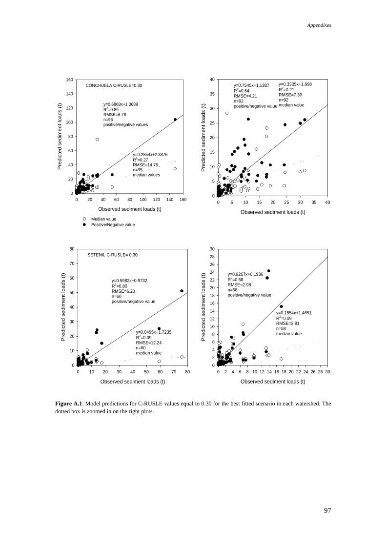
Appendixes
97
Figure A.1. Model predictions for C-RUSLE values equal to 0.30 for the best fitted scenario in each watershed. The
dotted box is zoomed in on the right plots.
Observed sediment loads (t)
0 20 40 60 80 100 120 140 160
Pre
dic
ted s
edim
ent lo
ads (
t)
0
20
40
60
80
100
120
140
160
Median value
Positive/Negative value
y=0.6808x+1.3689
R2=0.89
RMSE=6.78n=95positive/negative values
y=0.2854x+2.3876
R2=0.27
RMSE=14.76n=95median values
CONCHUELA C-RUSLE=0.30
Observed sediment loads (t)
0 5 10 15 20 25 30 35 40P
red
icte
d s
ed
ime
nt lo
ad
s (
t)
0
5
10
15
20
25
30
35
40
y=0.7545x+1.1387
R2=0.64
RMSE=4.21n=92positive/negative value
y=0.3305x+1.698
R2=0.21
RMSE=7.39n=92median value
Observed sediment loads (t)
0 10 20 30 40 50 60 70 80
Pre
dic
ted
se
dim
en
t lo
ad
s (
t)
0
10
20
30
40
50
60
70
80
y=0.5982x+0.9732
R2=0.80
RMSE=6.20n=60positive/negative value
y=0.0495x+1.7235
R2=0.09
RMSE=12.24n=60median value
SETENIL C-RUSLE= 0.30
Observed sediment loads (t)
0 2 4 6 8 10 12 14 16 18 20 22 24 26 28 30
Pre
dic
ted
se
dim
en
t lo
ad
s (
t)
0
2
4
6
8
10
12
14
16
18
20
22
24
26
28
30
y=0.9267x+0.1936
R2=0.58
RMSE=2.98n=58positive/negative value
y=0.1554x+1.4651
R2=0.09
RMSE=3.81n=58median value

Distributed processes in the runoff and sediment generation and transport in olive groves at different scales
98
Figure A.2. Model predictions for C-RUSLE values equal to 0.30 for the best fitted scenario in each watershed. The
dotted box is zoomed in on the right plots.
Observed sediment loads (t)
0 20 40 60 80 100 120 140 160
Pre
dic
ted
se
dim
en
t lo
ad
s (
t)
0
20
40
60
80
100
120
140
160
y=0.7886x+1.4536
R2=0.88
RMSE=5.95n=95positive/negative value
y=0.3071x+2.3135
R2=0.32
RMSE=14.25n=95median value
CONCHUELA Biweekly C-RUSLE
Observed sediment loads (t)
0 5 10 15 20 25 30 35 40
Pre
dic
ted
se
dim
en
t lo
ad
s (
t)
0
5
10
15
20
25
30
35
40
y=0.8825x+1.1729
R2=0.62
RMSE=5.10n=92positive/negative value
y=0.379x+1.5874
R2=0.20
RMSE=7.53n=92median value
Observed sediment loads (t)
0 10 20 30 40 50 60 70 80
Pre
dic
ted s
edim
ent lo
ads (
t)
0
10
20
30
40
50
60
70
80
y=0.5858x+0.6415
R2=0.70
RMSE=7.07n=60positive/negative value
y=0.0464x+1.5363
R2=0.09
RMSE=12.31n=60median value
SETENIL Biweekly C-RUSLE
Observed sediment loads (t)
0 2 4 6 8 10 12 14 16 18 20
Pre
dic
ted s
edim
ent lo
ads (
t)
0
2
4
6
8
10
12
14
16
18
20
y=0.7283x+0.3632
R2=0.40
RMSE=3.07n=57positive/negative value
y=0.1566x+1.2707
R2=0.11
RMSE=3.80n=57median value
99
REFERENCES
Abujamin, S., Abdurachman, A., Suwardjo, H. 1988. Contour grass strip as a low cost
conservation practice. In: Jantawar, S. (Editor), Soil erosion and its countermeasures.
Soil and Water Conservation Society of Thailand, Bangkok, pp. 112–118.
Al-wadaey, A., Wortmann, C.S., Franti, T.G., Shapiro, C.A., Eisenhauer, D.E. 2012.
Effectiveness of Grass Filters in Reducing Phosphorus and Sediment Runoff. Water
Air Soil Pollution 223: 5865–5875.
Bagarello, V., Baiamonte, G., Ferro, V., Giordano, G. 1993. Evaluating the topographic factors
for watershed soil erosion studies. In: Proc. Workshop on Soil Erosion in Semi-arid
Mediterranean Areas, (28-30 October, Taormina, Italy), ed R. P. C. Morgan.
Beaufoy, G. 2001. EU policies for olive farming. Unsustainable on all counts. BirdLife
Internacional-WWF, Brussels.
Bennet, H.H., Chapline, W.R. 1928. Soil erosion: a National menace. United States, Department
of Agriculture. Circular Nº 33.
Berglund, L. and Persson, L., 1996. Water repellence of cultivated organic soils. Acta
Agriculturae Scandinavica, Section B. Soil and Plant Science. 46: 145-152.
Bisdom, E.B.A., Dekker, L., Schoute, J.F. 1993. Water repellency of sive fractions from sandy
soils and relationships with organic material and soil structure. Geoderma. 56: 105-118.
Blackwell, P. 1993. Improving sustainable production from water repellent sands. Western
Australia Journal of Agriculture, 34: 158-167.
Blanco-Canqui, H., Lal, R. 2009. Extent of soil water repellency under long-term no-till soils.
Geoderma. 149: 171-180
Blanco-Canqui, H. 2011. Does no-till farming induce water repellency to soils? Soil Use and
Management. 27: 2-9.
Bodí, M., Mataix-Solera, J., Doerr, S.H., Cerdà, A. 2011. The wettability of ash from burned
vegetation and its relationship to Mediterranean plant species type, burn severity and
total organic carbon content. Geoderma, 160: 599-607.
Briante, R., Patumi, M., Terenziani, S., Bismuto, E., Febbraio, F., & Nucci, R., (2002). Olea
europaea L. leaf extract and derivatives: antioxidant properties. Journal of agricultural
and food chemistry. 50: 4934 - 4940.
100
Bronick, C.J., Lal, R., 2005. Manuring and rotation effects on soil organic carbon concentration
for different aggregate size fractions on two soils in northeastern Ohio, USA. Soil and
Tillage Research. 81: 239-252.
Cammeraat, L.H. 2004. Scale dependent thresholds in hydrological and erosion response of a
semi-arid catchment in southeast Spain. Agriculture, Ecosystems & Environment, 104:
317-332.
Cann, M., Lewis, D., 1994. The use of disperse sodic clay to overcome water repellence in
sandy soils in the South East of South Australia. Proceedings of the 2nd National Water
Repellence Workshop, 1-5 August, Perth, Western Australia. pp.49-57.
Castro, G., Romero, P., Gómez, J.A., Fereres, E., 2006. Rainfall redistribution beneath an olive
orchard. Agricultural Water Management. 86: 249-258.
Cerdà, A., Doerr, S., 2007. Soil wettability, runoff and erodibility of major dry-Mediterranean
land use types on calcareous soils. Hydrol. Process. 21: 2325–2336.
Cooley, K.R., Dedrick, A.R., Frasier, G.W. 1975. Water harvesting: state of the art. In:
Watershed Management Symposium. American Society of Civil Engineers Irrigation
and Drainage Division, Logan, UT. American Society of Civil Engineers, New York,
11–13 August 1975, 1–20.
Dearing, J.A. 1999. Environmental magnetic susceptibility. Using the Bartington MS2 System,
2nd Ed. Chi Publishing, England.
DeBano, L.F. 1975. Infiltration, evaporation and water movement as related to water repellency.
In: Soil Conditioners, Symposium Proceedings, Experimental Methods and Uses of Soil
Conditioners (W.C. Moldenhauer, Program Chairman). 15–16 November 1973. Las
Vegas, NV. Soil Science Society of America Special Publication Series 7. Madison,
WI. 155–163.
DeBano, L.F., Savage, S.M., Hamilton, D.A. 1976. The transfer of heat and hydrophobic
substances during burning. Soil Science Society of America Journal, 40: 779-782.
DeBano, L.F., 1981. Water repellent soils: a state-of-the-art, United States Department of
Agriculture, F.S., ed. (Berkeley (California), Pacific Southwest Forest and Range
Experiment Station), p. 21.
DeBano, L.F. 2000. Water repellency in soils: a historical overview. Journal of Hydrology, 231-
232.
Dekker, L.W., Ritsema, C.J. 1996. Preferential flow paths in a water repellent clay soil with
grass cover. Water Resources Research, 32: 1239-1249.
101
Deletic, A., Fletcher, TD. 2006. Performance of grass filters used for stormwater treatment—a
field and modelling study. Journal of Hydrology 317: 261–275
De Luna, E., Laguna, A., Giráldez, J.V. 2000. The role of olive trees in rainfall erosivity and
runoff and sediment yield in the soil beneath. Hydrology and Earth System
Sciences 4: 141–153.
De Vente, J., Poesen, J. 2005. Predicting soil erosion and sediment yield at the basin scale:
Scale issues and semi-quantitative models. Earth-Science Reviews 71: 95-125.
Doerr, S., 1998. On standardizing the ‘Water Drop Penetration Time’ and the ‘Molarity of an
ethanol droplet’ techniques to classify soil water repellency: a case study using medium
textured soils. Short communication. Earth Surf.Process.Landforms. 23: 663-668.
Doerr, S.H., Shakesby, R.A. and Walsh, R.P.D. 1998. Spatial variability of soil hydrophobicity
in fire-prone Eucalyptus and Pine forests, Portugal. Soil Science, 163: 313-324.
Doerr, S.H., Shakesby, R.A., Walsh, R.P.D. 2000. Soil water repellency: its causes,
characteristics, and hydro-geomorphological significance. Earth Science Reviews, 51:
33-65
Doerr, S.H., Thomas, A.D. 2000. The role of soil moisture in controlling water repellence: new
evidence from forest soils in Portugal. Journal of Hydrology. 231: 134-147.
Doerr, S.H., Ferreira, A., Walsh, R., Shakesby, R., Leighton-Boyce, G., Coelho, C. 2003. Soil
water repellency as a potential parameter in rainfall-runoff modelling: experimental
evidence at point to catchment scales from Portugal. Hydrological Processes, 17: 363-
377.
Di Stefano, C., Ferro, V., Palazzolo, E., Panno, M. 2005. Sediment delivery processes and
chemical transport in a small forested basin. Hydrological Sciences Journal 50, Issue 4.
Di Stefano, C., Ferro, V. 2007. Evaluation of the SEDD model for predicting sediment yield at
the Sicilian experimental SPA2 basin. Earth Surf. Process. Landforms 32: 1094-1109.
Duijsings, J. 1986. Seasonal variation in the sediment delivery ratio of a forested drainage basin
in Luxembourg. In: R.F. Hadley (Ed.), Drainage Basin Sediment Delivery, IAHS
Publication 159, IAHS Press, Wallingford, 153–164.
European Environment Agency. www.eea.europa.eu
EES Engineering Equation Solver, F-Chart Software: Engineering Software, 2008. Madison,
WI, USA.
102
ESRI, 2006. ArcGIS 9.3 GIS. Environmental Systems Research Institute, Inc., Redlands, CA,
USA.
Fernández, C., Wu, J.Q., McCool, D.K., Stockle, C. 2003. Estimating water erosion and
sediment yield with GIS, RUSLE and SEDD. Journal of Soil and Water conservation
58: 128-136.
Ferro,V., Minacapilli, M. 1995. Sediment delivery processes at basin scale. Hydrological
Sciences Journal 40, Issue 6.
Ferro, V. 1997. Further remarks on a distributed approach to sediment delivery. Hydrological
Sciences Journal 42, Issue 5.
Ferro, V., Porto, P. 1998. Testing a distributed approach for modelling sediment delivery.
Hydrological Sciences Journal 43, Issue 3.
Ferro, V., Porto, P. 2000. Sediment Delivery Distributed (SEDD) model. Journal of Hydraulic
Engineering, Vol. 5, No. 4.
Food and Agriculture Organization of the United Nations (FAOSTAT), 2012.
www.faostat.fao.org
Fox, J., Papanicolau, A. 2008. An un-mixing model to study watershed erosion processes. IIHR-
Hydroscience and Engineering, University of Iowa, Iowa City, IA 52242, USA
Fox, G. A.; Penn, C. J. 2013. Empirical model for quantifying total phosphorus reduction by
vegetative filter strips. Transactions of the ASABE 56: 1461–1469.
Francia, A., Durán, V., Martínez, A. 2006. Environmental impact from mountainous olive
orchards under different soil-managment systems (SE Spain). Sci. Total Environ, 358:
46-60.
Franco, J.A., Calatrava, J. 2012. The difussion process of no-tillage with herbicides application
in Southern Spain’s olive groves. Journal of Environmental Planning and Management,
55: 979-1003.
Fu, G., Chen, S., McCool, D. 2006. Modeling the impacts of no-till practice on soil erosion and
sediment yield with RUSLE, SEDD and ArcView GIS. Soil & Tillage Research 85: 38-
49.
Fu, C., Ruan, B., Gao, T. 2013. Watershed Agricultural Non-Point Source Pollution
Management. Pol. J. Environ. Stud. 22: 367-375.
103
Gabriels, D., Moldenhauer, W.C. 1978. Size distribution of eroded material from simulated
rainfall: effect over a range of texture. Soil Sci. Soc. Am. J. 42: 954– 958.
García Marín, A. P. 2007. Análisis multifractal de series de datos pluviométricos en Andalucía.
PhD Thesis. Departamento de Ingeniería Rural. Universidad de Córdoba.
Gómez, J.A., Giráldez, J.V., Fereres, E., 1999. Effects of tillage method on soil physicial
properties infiltration and yield in an olive orchard. Soil Till. Res. 52: 167-175.
Gómez, J.A., Giráldez, J.V., Fereres, E., 2001. Rainfall interception by olive trees in relation to
leaf area. Agricultural Water Management. 55: 65-76.
Gómez, J.A., Vanderlinden, K., Giráldez, J.V., Fereres, E., 2002. Rainfall concentration under
olive trees. Agricultural Water Management. 55: 53-70.
Gómez, J.A., Orgaz, F., Villalobos, J., Fereres, E. 2002. Analysis of the effects of soil
management on runoff generation in olive orchards using a physically based model.
Soil Use Manage. 18: 191-198.
Gómez, J.A., Battany, M., Renschler, C.S., Fereres, E. 2003. Evaluating the impact of soil
management on soil loss in olive orchards. Soil Use Manage. 19: 127- 134.
Gómez, J.A., Romero, P., Giráldez, J.V., Fereres, E. 2004. Experimental assessment of runoff
and soil erosion in an olive grove on a Vertic soil in southern Spain affected by soil
management. Soil Use Manage. 20: 426-431.
Gómez, J.A., Sobrinho, T.A, Giráldez, J.V., Fereres, E. 2009. Soil management effects on
runoff, erosion and soil properties in an olive grove of Southern Spain. Soil & Tillage
Research 102: 5–13.
Gómez, J.A., Guzmán, M.G., Giráldez, J.V., Fereres, E. 2009. The influence of cover crops
and tillage on water and sediment yield, and on nutrient, and organic matter losses
in an olive orchard on a sandy loam soil. Soil Till Res 106: 137–144.
Gómez, J.A., Giráldez, J.V., 2010. Erosión y degradación de suelos, in: Gómez, J.A. (Ed.),
Sostenibilidad de la producción de olivar en Andalucía. Consejo Superior de
Investigaciones Científicas, Madrid, pp. 45-86.
Gómez, J.A., Taguas, E.V., Vanwalleghem, T., Pérez-Alcántara, R. 2010. Effect of large rainfall
events on runoff and soi losses in two small experimental agricultural catchments in
Southern Spain. Geophysical Research Abstracts. Vol. 12, EGU2010-6021.
104
Gómez, J.A., Llewellyn, C., Basch, G., Sutton, P. B., Dyson, J. S., Jones, C. A. 2011. The
effects of cover crops and conventional tillage on soil and runoff loss in vineyards and
olive groves in several Mediterranean countries. Soil Use and Management 27: 502 –
514.
Gómez, J.A., Taguas, E.V., Vanwalleghem, T., Giráldez, J.V., Sánchez, F., Ayuso, J.L., Lora,
A., Mora, A. 2011. Criterios técnicos para el control de cárcavas, diseño de muros de
retención y revegetación de paisajes agrarios. Manual del operador en inversiones no
productivas. Sevilla: Consejería de Agricultura y Pesca, Servicio de Publicaciones y
Divulgación.
Gómez, J.A., Vanwalleghem, T., De Hoces, A., Taguas, E.V. 2014. Hydrological and erosive
response of a small catchment under olive cultivation in a vertic soil during a five-year
period: Implications for sustainability. Agriculture, Ecosystems and Environment 188:
229-244.
Gómez-Limón J.A., Picazo-Tadeo A.J., Reig-Martínez E. 2011. Eco-efficiency assessment of
olive farms in Andalusia. Land Use Policy 29: 395– 406.
González-Peñaloza, F., Cerdà, A., Zavala, L., Jordán, A., Giménez-Morera, A., Arcenegui, V.,
2012. Do conservative agriculture practice increase soil water repellency? A case study
in citrus-cropped soils. Soil & Tillage Research. 124: 233-239.
Guzmán, G., Barron, V., Gomez, J.A. 2010. Evaluation of magnetic iron oxides as sediment
tracers in water erosion experiments. Catena 82: 126–133.
Guzmán, G., Barrón, V., Gómez, J.A. 2010. Evaluation of magnetic iron oxides as sediment
tracers in water erosion experiments. Catena 82: 126–133.
Guzmán, G., Gómez, J.A. Giráldez, J.V. 2010. Measurement of particle size distribution of
soil and selected aggregate sizes using the hydrometer method and laser diffractometry.
Geophysical Research Abstracts Vol. 12, EGU2010-4422-1. EGU General Assembly
2010.
Guzmán, G. 2011. Desarrollo de trazadores de suelo para el estudio del arrastre y redistribución
de sedimentos debidos a la erosión hídrica. PhD Thesis. Departamento de Agronomía.
Universidad de Córdoba.
Guzmán, G., Vanderlinden, K., Giráldez, J.V., Gómez, J.A. 2013. Assessment of Spatial
Variability in Water Erosion Rates in an Olive Orchard at Plot Scale using a Magnetic
Iron Oxide Tracer. Soil Sci. Soc. Am. J. 77: 350–361.
Heathwaite, A., Quinn, P., Hewett, C. 2005. Modelling and managing critical source areas of
diffuse pollution from agricultural land using flow connectivity simulation. Journal of
Hydrology, 304: 446-461.
105
Hernández, A.J., Lacasta, C., Pastor, J. 2005. Effects of different management practices on soil
conservation and soil water in a rainfed olive orchard. Agricultural Water Management,
77: 232-248.
Instituto de Investigación y Formación Agraria y Pesquera (IFAPA).2013. Consejería de
Agricultura, Pesca y Medio Ambiente.
IUSS Working Group WRB. 2006. World reference base for soil resources 2006. World Soil
Resources Reports No. 103. FAO, Rome.
Jain, M., Kothyari, U. 2000. Estimation of soil erosion and sediment yield using GIS. J. Soils
Sediments 45, Issue 5.
Jin, C., Römkens, M.J.M. 2000. Experimental studies of factors in determining sediment
trapping in vegetative filter strips. Trans. ASAE 44: 277–288.
Jordán, A., Zavala, L., González, F., Bárcenas-Moreno, G., Mataix-Solera, J. 2010. Repelencia
al agua en suelos afectados por incendios: métodos sencillos de determinación e
interpretación. In: Cerdà, A. and Jordán, A. (Eds): Actualización en métodos y técnicas
para el estudio de los suelos afectados por incendios forestales. FUEGORED, Càtedra
de Divulgació de la Ciència, Universitat de València, Spain. 521 pp.
Kapil, A., Mickelson, S.K., Helmers, M.J., Baker, L.L. 2010. Review of Pesticide Retention
Processes Occurring in Buffer Strips Receiving Agricultural Runoff. Journal of the
American Water Resources Association 46: 618–647.
Keizer, J.J., Doerr, S.H., Malvar, M.C., Ferreira, A., Pereira, V.M.F.G., 2007. Temporal and
spatial variations in topsoil water repellence throughout a crop-rotation cycle on sandy
soil in north-central Portugal. Hydrol. Process. 21: 2317-2324.
Kirkby, M. 1980. The problem. In Kirkby, M., and Morgan, R.P.C. (Eds), Soil Erosion. John
Wiley & Sons, 311 pp.
Kirkby, M., Imeson, A., Bergkamp, G., Cammeraat, L.H. 1996. Scaling up processes and
models from the field plot to the watershed and regional areas. Journal of Soil & Water
Conservation. 51:391-395.
Kirkby, M., et al., 2004. Pan-European soil erosion risk assessment: The PESERA MAP
Version 1 October 2003. Special Publication, ISPRA Nº 73. S.P.I. 04.73.
Koiter, A.J., Owens, P.N., Petticrew, E.L., Lobb, D.A. 2013. The behavioural characteristics
of sediment properties and their implications for sediment fingerprinting as an approach
for identifying sediment sources in river basins. Earth-Science Reviews 125: 24–42.
106
Kosmas, C., Danalatos, N., Cammeraat, L.H., Chabart, M., Diamantopoulos, J., Farand, L.,
Gutiérrez, L., Jacob, A., Marqués, H., Martínez-Fernández, J., Mizara, A., Moustakas,
N., Nicolau, J.M., Oliveros, C., Pinna, C., Puddu, R., Puigdefábregas, J., Roxo, M.,
Simao, A., Stamou, G., Tomasi, N., Usai, D., Vacca, A. 1997. The effect of land use on
runoff and soil erosion rates under Mediterranean conditions. Catena 29: 45-60.
Kruskal, W.H. and Wallis, W.A., 1952. Use of ranks in one-criterion variance analysis. Journal
of the American Statistical Association. 47: 2583-621.
Lascelles, B., Favis-Mortlock, D.T., Parsons, A.J., Guerra, A. 2000. Spatial and temporal
variation in two rainfall simulators: implications for spatially explicit rainfall simulation
experiments. Earth Surf. Process. Landforms 25: 709-721.
Leighton-Boyce, G., Doerr, S.H., Shakesby, R., Walsh, R., Ferreira, A., Boulet, A.K., Coelho,
C. 2005. Temporal dynamics of water repellency and soil moisture in eucalypt
plantations, Portugal. Soil Research, 43: 269–280.
Le Bissonaiss, Y., Lecomte, V., Cerdan, O. 2004. Grass strip effects on runoff and soil loss.
Agronomie 24: 129–136.
Letey, J., Osborn, J., Pelishek, R.E. 1962. The influence of the water-solid contact angle on
water movement in soil. International Association of Scientific Hydrology. Bulletin, 7:
75-81
Letey, J. 1969. Measurements of contact angle, water drop penetration time, and critical surface
tension. In: Symposium on water-repellent soils, Proceeding, May 6-10, 1968,
University of California, Riverside, 43-47, March 1969.
Letey, J., 2000. Causes and consequences of fire-induced soil water repellency. Hydrol. Process.
15: 2867–2875.
Licciardello, F., Taguas, E.V., Barbagallo, S., Gómez, J.A. 2013. Application of the water
erosion prediction project (WEPP) in olive orchards on Vertic soil with different
management conditions. Transactions of the ASABE 56: 951-961.
Lidgi, E., Morgan, R.P.C. 1995. Contour grass strips: a laboratory simulation of their role in
soil erosion control. Soil Technology 8: 109–117.
López-Cuervo, S. 1990. La erosión en los suelos agrícolas y forestales de Andalucía. Colección
Congresos y Jornadas N 17/1990, 11-16. Junta de Andalucía. Consejería de Agricultura
y Pesca.
López-Moreno, J.L., Beguería, S., García-Ruíz, J.M. 2004. The management of a large
Mediterranean reservoir: storage regimens of the Yesa Reservoir, Upper Aragon River
Basin, Central Spanish Pyrenees. Environmental Management, 34: 508-5015
107
López-Vicente, M., Navas, A., 2010. Relating soil erosion and sediment yield to geomorphic
features and erosion processes at the catchment scale in the Spanish Pre-Pyrenees.
Environ. Earth Sci. 61: 143-158.
López-Vicente, M., Lana-Renault, N., García-Ruíz, J.M., Navas, A. 2011. Assessing the
potential effect of different land cover management practices on sediment yield from an
abandoned farmland catchment in the Spanish Pyrenees. J. Soils Sediments 11: 1440-
1455.
López-Vicente, M., Poesen, J., Navas, A., Gaspar, L. 2013. Predicting runoff and sediment
connectivity and soil erosion by water for different land use scenarios in the Spanish
Pre-Pyrenees. Catena 102, 62-73.
Lozano-García, B., Parras-Alcántara, L. 2014. Variation in soil organic carbon and nitrogen
stocks along a toposequence in a traditional Mediterranean olive grove. Land Degrad.
Dev., 25: 297-304.
Lu, H., Moran, C.J., Sivapalan, M. 2005. A theoretical exploration of catchment-scale sediment
delivery. Water Resources Research 41, W09415.
Ma, L., Pan, C., Teng, Y., Shangguan, Z. 2013. The performance of grass filter strips in
controlling high-concentration suspended sediment from overland flow under
rainfall/non-rainfall conditions. Earth Surf. Process. Landforms 38: 1523–1534.
Ma'shum, M., Oades, J.M., Tate, M.E. 1989. The use of dispersible clays to reduce water
repellency of sandy soils. Australian Journal of Soil Research. 27: 797-806.
MacDonald, L.H., Sampson, R.W., Anderson, D.M. 2001. Runoff and road erosion at the plot
and road segment scales, St. John, US Virgin Islands. Earth Surf. Process.
Landforms 26, 251-272.
Malam I., O., Le Bissonnais, Y., Planchon, O., Favis-Mortlock, D., Silvera, N., Wainwright, J.
2006. Soil detachment and transport on field-and laboratory-scale interrill areas: erosion
processes and the size-selectivity of eroded sediment. Earth Surf. Process. Landforms
31: 929–939.
Mankin, K., Ngandun, D., Barden, C., Hutchinson, S., Geyer, W. 2007. Grass-shrub riparian
buffer removal of sediment, phosphorus, and nitrogen from simulated runoff. Journal
of the American water resources association 43: 1108–1116.
Martínez-Mena, M., Alvarez Rogel, J., Albaladejo, J., Castillo, V. 1999. Influence of vegetal
cover on sediment particle size distribution in natural rainfall conditions in a semiarid
environment. Catena 38: 175–190.
108
Martínez, A., Durán, V.H., Francia, J.R. 2006. Soil erosion and runoff response to plant-
cover strip son semiarid slopes (SE Spain). Land Degrad. Develop 17: 1–11.
Martz, L.W., de Jong, E. 1991. Using Cs-137 and landform classification to develop a net soil
erosion budget for a small Canadian prairie watershed. Catena 18: 298–308.
Märker, M., Angeli., L., Bottai, L., Constantini, E., Ferrari, R., Inocenti, L., Siciliano, G. 2008.
Assessment of land degradation susceptibility by scenario analysis: a case study in
Southern Tuscany, Italy. Geomorphology 93, 120-129. Geophysical Research
Abstracts, Vol. 15, EGU2013-6380. EGU General Assembly 2013
Ma'shum, M., Oades, J.M., Tate, M.E. 1989. The use of dispersible clays to reduce water
repellency of sandy soils. Australian Journal of Soil Research. 27, 797-806.
Merrit, W.S., Letcher, R.A., Jakeman, A.J. 2003. A review of erosion and sediment transport
models. Environmental Modelling & Software 18: 761-799.
McGhie, D.A., Posner, A.M. 1981. The effect of plant top material on the water repellence of
fire sands and water repellent soils. Australian Journal of Agriculture Research, 32:
609-620.
McKissock, E.L., Walker, R.J., Gilkes, D.J. Carter., 2000. The influence of clay type on
reduction of water repellency by applied clays: a review of some West Australian work.
J. Hydrol., 231–232, pp. 323–332.
Moore, I. D., Burch, F. J. 1986 Physical basis of the length-slope factor in the universal soil loss
equation. Soil Sci. Soc. Am. J. 50: 1294-1298.
National Statistic Institute (INE), 2009. www.ine.es
Nash, J.E., Sutcliffe, J.V. 1970. River flow forecasting through conceptual models. J. Hydrol.
10, 280-292.
Nelson, D.W. and Sommers, L.E., 1982. Total carbon, organic carbon and organic matter, in:
Miller, R.H., Keeney, D.R. (Eds.), Methods of soil analysis, Part 2. Chemical and
microbiological properties, Agronomy Monograph. 9: 539-579. ASA & SSSA,
Madison, WI.
Onstad, C., Foster, G. 1975. Erosion modeling on a watershed. Trans. ASAE, 18: 288-292.
Palese, A.M., Vignozzi, N., Celano, G., Agnelli, A.E., Pagliai, M., Xiloyannis, C. 2014.
Influence of soil management on soil physical characteristics and water storage in a
mature rainfed olive orchard, Soil and Tillage Research 144: 96-109.

109
Pan, C., Ma, L., Shangguan, Z. 2010. Effectiveness of grass strips in trapping suspended
sediments from runoff. Earth Surf. Process. Landforms 35: 1006–1013.
Pankau, R.C., Schoonover, J.E., Williard, K.W.J., Edwards, P.J. 2012. Concentrated flow
paths in riparian buffer zones of southern Illinois. Agroforestry System 84: 191–205.
Parsons, A.J., Wainwright, J., Brazier, R.E. and Powell, D.M., 2006. Is sediment delivery a
fallacy? Earth Surface Processes and Landforms, 31: 1325-1328.
Pastor, M., Castro, V., Vega, V., Humanes, M. 1999. Sistema de manejos de suelo. In:
Barranco, D., Fernández, R., Rallo, L. Eds. El cultivo del olivo. Madrid, Spain. Mundi
Prensa: 198-228.
Pedrera-Parrilla, A., Martínez, G., Espejo-Pérez, A., Gómez, J.A., Giráldez, J.V., Vanderlinden,
K. 2014. Mapping impaired olive tree development using electromagnetic induction
surveys. Plant and Soil 384: 381-400.
Peragón. J., 2012. Time course of pentacyclic triterpenoids from fruits and leaves of olive tree
(Olea europaea L) cv. Picual and cv. Cornezuelo during ripening. J. Agric. Food Chem.
61: 6671–6678.
Piest, R.F., Kramer, L.A., Heineman, H.G. 1975. Sediment movement from loessial watersheds.
U.S. Dep. Agric., Publ., ARS-S-40: 130–141
Pimentel, D., Harvey, C., Resosudarmo, P., Sinclair, K., Kurz, D., McNair, M., Crist, S.,
Shpritz, L., Fitton, L., Saffouri, R., Blair, R. 1995. Environmental and Economic Costs
of Soil Erosion and Conservation Benefits. Science, New Series, 267: 1117-1123.
Renard, K.G., Foster, G.R., Weesies, G.A., McCool, D.K., Yoder, D.C., 1997. Predicting soil
erosion by water: a guide to conservation planning with the Revised Universal Soil Loss
Equation (RUSLE). Handbook Nº. 703. US Department of Agriculture, 404 pp.
Renschler, C., Harbor, J. 2000. Soil erosion assessment tools from point to regional scales –the
role of geomorphologists in land management research and implementation.
Geomorphology, 47: 189-209.
Robinson, D., 1999. A comparison of soil-water distribution under ridge and bed cultivated
potatoes. Agricultural Water Management. 42: 189-204.
Romero, P., Castro, G., and Gómez, J.A., 2007. Curve number values for olive orchards under
different soil management. Soil Science Society of America Journal. 71: 1758-1769.
Römkens, M., Wang, J. 1986. Effect of tillage on surface roughness, Trans. ASAE 29, 429–
433.
110
Savage, S.M. 1974. Mechanism of fire-induced water repellency in soil. Soil Science Society of
America Proceedings, 38: 652-657.
Savage, S.M., Martin, J.P., Letey, J., 1969. Contribution of some soil fungi to natural and heat-
induced water repellence in sand. Soil Science Society of America Proceedings. 33:
405-409.
Scholl, D.G., 1971. Soil wettability in Utah juniper stands. Soil Science Society of America
Proceeding. 35: 344-345.
Selby, M.J. 1993. Hillslope materials and processes. Oxford University Press, 1982 pp
Seeger, M. 2007. Uncertainty of factors determining runoff and erosion processes as quantified
by rainfall simulations. Catena 71: 56–67.
Shakesby, R.A., Doerr, S.H., Walsh, R.P.D., 2000. The erosional impact of soil hydrophobicity:
current problems and future research directions. Journal of Hydrology. 231-232: 178-
191.
Sistema de Información Agroclimática para el Regadío (SIAR). Ministerio de Agricultura,
alimentación y medio ambiente. 2013.
SPSS Inc. Released 2009. PASW Statistics for Windows, Version 17.0. Chicago: SPSS Inc.
Stevens C.J., Quinton J.N. (2008) Investigating source areas of eroded sediments transported in
concentrated overland flow using rare earth element tracers. Catena 74: 31–36.
Stiti, N., Hartmann, M. A., 2012. Nonsterol triterpenoids as major constituents of Olea
europaea. Journal of lipids.
Taguas, E.V. 2007. Evaluación de la pérdida de suelo en olivar a escala de microcuenca bajo
distintos manejos de suelo. PhD. University of Córdoba.
Taguas, E. V., A. Peña, J. L. Ayuso, Y. Yuan, and R. Pérez. 2009. Evaluating and modelling the
hydrological and erosive behaviour of an olive orchard microcatchment under non–
tillage with bare soil in Spain. Earth Surf. Proc. and Land 34: 738-751.
Taguas, E.V., Peña, A., Ayuso, J.L., Pérez, R., Yuan, Y., Giráldez, J.V. 2010. Rainfall
variability and hydrological and erosive response of an olive tree microcatchment under
no tillage with a spontaneous grass cover in Spain. Earth Surf Process Land 35: 750-
760.
111
Taguas, E.V., Moral, C., Ayuso, J.L., Pérez, R., Gómez, J.A. 2011. Modeling the spatial
distribution of water erosion within a Spanish olive orchard microcatchment using the
SEDD model. Geomorphology 133: 47-56.
Taguas, E.V., Burguet, M., Pérez, R., Ayuso, J.L., Gómez, J.A., 2012. Interpretation of the
impact of different managements and the rainfall variability on the soil erosion in a
Mediterranean olive orchard microcatchment. Geophysical Research Abstracts 14,
EGU2012-10966.
Taguas, E.V., Gómez, J.A. 2015. Vulnerability of olive orchards under the current CAP
(Common Agricultural Policy) regulations on soil erosion: a study case in Southern
Spain. Land Use Policy 42: 683-694.
Thayer, C.A., Gilley, J.E., Durso, L.M., Marx, D.B. 2012. Wheat strips effects on nutrient
loads following manure applications. Transactions of the ASABE 55: 439–449.
Thornes, J. 1980. Erosional processes of running water and their spatial and temporal controls: a
theoretical viewpoint. In Kirkby, M. and Morgan, R. (Eds): Soil Erosion. John Wiley &
Sons, Ltd. British Geomorphological Research Group.
Ulrich, U., Dietrich, A., Fohrer, N. 2013. Herbicide transport via surface runoff during
intermittent artificial rainfall: A laboratory plot scale study. Catena, 101: 38-49.
Urbanek, E., Hallet, P., Feeney, D., Horn, R., 2007. Water repellency and distribution of
hydrophilic and hydrophobic compounds in soil aggregates from different tillage
systems. Geoderma. 140: 147-155.
van Dijk, P.M., Kwaad, F.J.P., Klapwijk, M. 1996. Retention of water and sediment by grass
strips. Hydrological Processes 10: 1069–1080.
Vanwalleghem, T., Infante, J.A., González, M., Soto, D., Gómez, J.A. 2011. Quantifying the
effect of historical soil management on soil erosion rates in Mediterranean olive
orchards. Agriculture, Ecosystems & Environment 142: 341-351.
Wallbrink, P.J., Murray, A.S. 1993. Use of fallout radionuclides as indicators of erosion
processes. Hydrological Processes 7: 297–304.
Walling, D.E. 1983. The sediment delivery problem. Journal of Hydrology 65: 209-237.
Walling, D.E., He, Q. 1999. Using fallout lead-210 measurements to estimate soil erosion on
cultivated land. Sci. Soc. Am. J. 63: 1404–1412.
112
Wander, I. W. (1949). An interpretation of the cause of water-repellent sandy soils found in
citrus groves of central Florida. Science, 2856: 299-300.
Watson, C.L., Letey, J. 1970. Indices for characterizing soil-water repellency based upon
contact angle surface tension relationships. Soil Science Society of America
Proceedings, 34: 841-844.
Williams, J.R. 1977. Sediment delivery ratios determined with sediment and runoff models. Int.
Assoc. Hydrol. Sci. Publ. 122: 168-179.
Wischmeier, W.H., Smith, D.D. 1978. Predicting Rainfall Erosion Losses. A guide to
conservation planning. Agriculture Handbook Nº 537. USDA-SEA, Govt. Printing
Office, Washington D.C.
Xiao, B., Wang, Q., Wang, H., Dai, Q., Wu, J. 2011. The effects of narrow grass hedges on soil
and water loss on sloping lands with alfalfa (Medicago sativa L.) in Northern China.
Geoderma 167-168: 91–102.
Zavala, L., González, F.A., Jordán, A., 2009. Intensity and persistence of water repellency in
relation to vegetation types and soil parameters in Mediterranean SW Spain. Geoderma.
152: 361-374.
Zhang, X.C., Friedrich, J.M., Nearing, M.A., Norton, L.D. 2001. Potential use of rare earth
oxides as tracers for soil erosion and aggregation studies. Soil Science Society of
America Journal 65: 1508–1515.
Ziogas, A., Dekker, L., Oostindie, K., Ritsema, C.J., 2005.Soil water repellency in north-eastern
Greece with adverse effects of drying on the persistence. Australian Journal of Soil
Research. 43: 281-289.