Embed Size (px)
Citation preview

Kuldeep Virdi and Lauri Tenhunen (Editors)
Proceedings of the METNET Seminar 2011 in Aarhus
Metnet Annual Seminar in Aarhus University, Denmark on 12 – 13 October 2011

Proceedings of the METNET Seminar 2011 in Aarhus
Kuldeep Virdi and Lauri Tenhunen (Editors)

HAMK University of Applied Sciences
Proceedings of the METNET Seminar 2011 in Aarhus
Kuldeep Virdi and Lauri Tenhunen (Editors)

Editors:Kuldeep Virdi, Aarhus UniversityLauri Tenhunen, HAMK University of Applied Sciences
Proceedings of the METNET Seminar 2011 in Aarhus held at Aarhus University on 12 – 13 October 2011
ELEcTrOniciSBn 978-951-784-555-7 (PDF)iSSn 1795-424X HAMKin e-julkaisuja 12/2011
PrinTEDiSBn 978-951-784-556-4iSSn 1795-4231 HAMKin julkaisuja 8/2011
© HAMK UAS and writers
PUBLISHERHAMK University of Applied SciencesPO Box 230 Fi-13101 Hämeenlinna, FinLAnDtel. +358 3 [email protected]/julkaisut
This publication has been produced in cooperation with the rOcKET project, which is partly financed by the European regional Development Fund.
Hämeenlinna, October 2011

5Proceedings of the METNET Seminar 2011 in Aarhus
Index
Technical Papers .................................................................................................................... 7
Dan Dubină, Viorel Ungureanu & Andrei CrişanINTERACTIVE BUCKLING OF COLD-FORMED STEEL SECTIONS APPLIED IN PALLET RACK UPRIGHT MEMBERS ...................................................................................... 8
Rauno Toppila, Jakub Dolejs, Timo Kauppi, Tomas Brtnik, Jukka Joutsenvaara, Pauli Vaara & Raimo Ruoppa INVESTIGATION OF BEHAVIOUR OF HSS USING ADVANCED TECHNIQUES ..................... 24
Mikko Salminen & Karol BzdawkaCATENARY ACTION AND STRAINS OF WQ-BEAM IN OFFICE BUILDING DURING FIRE ... 37
Keijo Fränti, Hilkka Ronni & Markku HeinisuoEFFECT OF ZINC COATING ON STEEL TEMPERATURES AT ELEVATED TEMPERATURES .. 50
Hilkka Ronni, Henri Perttola & Markku HeinisuoEXPERIMENTS OF END PLATE JOINTS IN AMBIENT AND FIRE CONDITIONS UNDER BIAXIAL BENDING .............................................................................................................. 58
Patrik Takács, László Horváth & István SzontaghFIRE DESIGN OF A STEEL HALL WITHOUT FIRE PROTECTION ........................................ 74
Josef Machacek & Martin CharvatLONGITUDINAL SHEAR IN STEEL AND CONCRETE COMPOSITE BRIDGE TRUSSES ......... 85
Hayder H. Alkhudery & Kuldeep S. VirdiBEHAVIOUR OF METAL FOAM SANDWICH PANELS ........................................................... 97
Stelian Brad, Adrian Chioreanu & Zsolt NagyPRODUCT INNOVATION IN SMES: A WEB-BASED SUPPORTING TOOL AND CASE STUDIES .................................................................................................................... 110
Lauri TenhunenON THE COST STRUCTURES IN STEEL CONSTRUCTION .................................................. 123
6 Proceedings of the METNET Seminar 2011 in Aarhus
Technical Notes .................................................................................................................. 135
Helmuth Köber, Bogdan Ştefănescu & Şerban DimaPOTENTIALLY PLASTIC ZONES CONFIGURATIONS IN BOTTOM COLUMNS OF ECCENTRICALLY BRACED FRAMES .................................................................................. 136
Selyantsev I. & Tusnin A.THE INFLUENCE OF CROSS-SECTION SHAPE CHANGING ON WORK OF THIN WALLED COLD-FORMED STEEL BEAM. ........................................................................................... 143
Helmuth Köber, Bogdan Ştefănescu & Şerban DimaCOMMENTS ABOUT THE DESIGN OF RUNWAY GIRDERS ACCORDING TO NEW EN STANDARDS ..................................................................................................................... 149
Tusnin Alexander & Tusnina Olga ANALYSIS SUPERCRITICAL BEHAVIOR OF ROD SYSTEMS .............................................. 160
Sustainability Issues .......................................................................................................... 170
Olli IlveskoskiSUSTAINABILITY - NEED FOR A NEW APPROACH IN THE ARCHITECTURE ..................... 171

7Proceedings of the METNET Seminar 2011 in Aarhus
TECHNICAL PAPERS

8 Proceedings of the METNET Seminar 2011 in Aarhus
INTERACTIVE BUCKLING OF COLD-FORMED STEEL SECTIONS APPLIED IN PALLET RACK UPRIGHT
MEMBERS
Dan Dubină
Viorel Ungureanu
Andrei Crişan
„POLITEHNICA” University of Timişoara
Abstract
Thin-walled cold-formed steel performance is influenced by the presence of imperfections, which could be of geometric or mechanical type, the local or sectional instability, the global instability and the interaction of these two instability modes. In the case of perforated section, these factors are supplemented by the presence of perforations, which in some way, can be regarded also as imperfections. Due to the wide variety in the size and configuration of perforations, it is impossible to provide a unified practical design procedure to calculate the ultimate strength of perforated sections. Generally, the design codes do not contain specific analytical methods for these sections, but for a design assisted by testing. This is the case of European Norm, EN1993-1-3 and Australian and New Zeeland standard AS/NZS4600:2005. In contrast, the North American Specification (AISI:2004) provides specific recommendations for perforated sections, but they have got some limitations regarding the size and shape of perforations and the distance between them (e.g. hole diameter and pitch).
In the case of storage racking there are specific design rules and standards, such as Recommendations of the Federation Europeenne de la Manutention (FEM 10.2.02, replaced in 2009 by the EN15512:2009 standard), Australian Standard (AS4048:1993) and Specification for the Design, Testing and Utilisation of Industrial Steel Storage Racks by the Rack Manufacturers Institute (MH16.1:2008). All these codes, recommend experimental tests to evaluate the ultimate strength of rack members. However, testing is costly and time consuming, and, if available, simplified design approaches would be preferred. Nowadays, numerical procedures like Finite Element Methods, Finite Strip Method or Generalised Beam Theory have been successfully used to predict behaviour of perforated sections. However, the numerical models need to be calibrated by relevant tests.
The present paper proposes, after discussing the interactive buckling phenomena, a calculation procedure to design perforated sections. This approach applies the ECBL method to clibate a specific imperfection factor for the European buckling curves.
9Proceedings of the METNET Seminar 2011 in Aarhus
Simple and Coupled Instabilities
Steel sections may be subject to one of four generic types of buckling, namely local, global, distortional and shear.
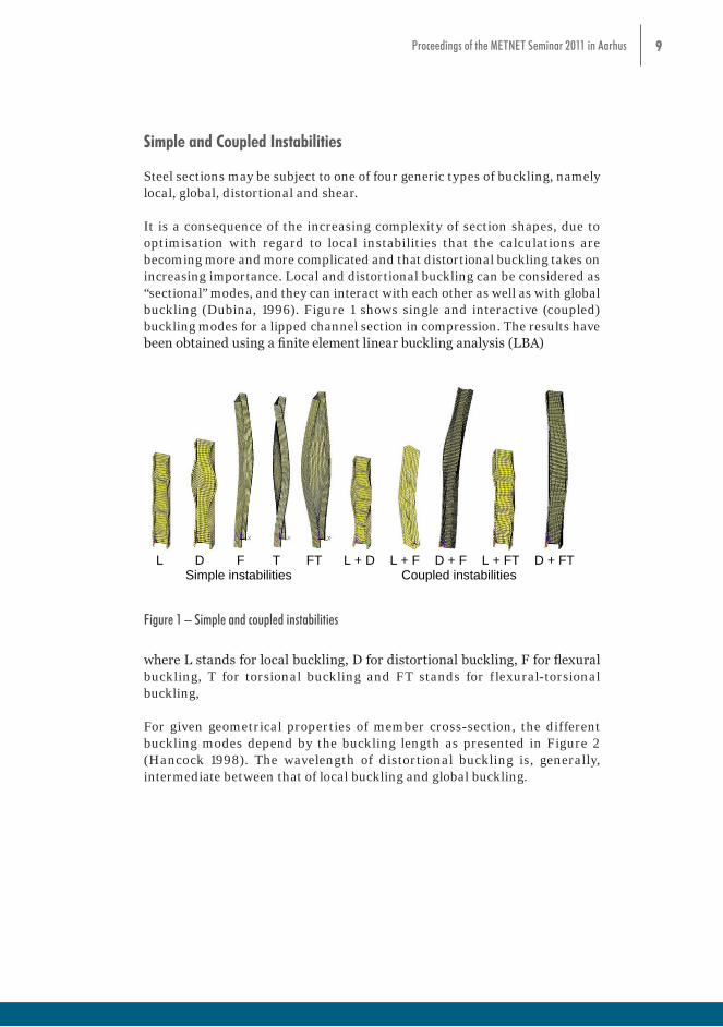
It is a consequence of the increasing complexity of section shapes, due to optimisation with regard to local instabilities that the calculations are becoming more and more complicated and that distortional buckling takes on increasing importance. Local and distortional buckling can be considered as “sectional” modes, and they can interact with each other as well as with global buckling (Dubina, 1996). Figure 1 shows single and interactive (coupled) buckling modes for a lipped channel section in compression. The results have been obtained using a finite element linear buckling analysis (LBA)
It is a consequence of the increasing complexity of section shapes, due to optimisation with regard to local instabilities that the calculations are becoming more and more complicated and that distortional buckling takes on increasing importance. Local and distortional buckling can be considered as “sectional” modes, and they can interact with each other as well as with global buckling (Dubina, 1996). Figure 1 shows single and interactive (coupled) buckling modes for a lipped channel section in compression. The results have been obtained using a finite element linear buckling analysis (LBA)
L D F T FT L + D L + F D + F L + FT D + FT Simple instabilities Coupled instabilities
Figure 1 – Simple and coupled instabilities
where L stands for local buckling, D for distortional buckling, F for flexural buckling, T for torsional buckling and FT stands for flexural-torsional buckling,
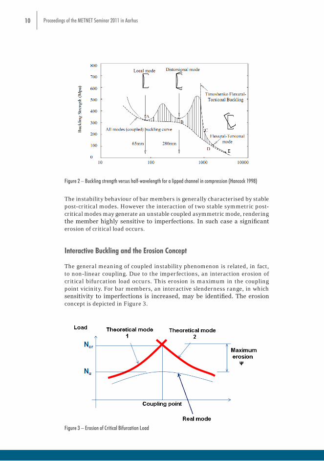
For given geometrical properties of member cross-section, the different buckling modes depend by the buckling length as presented in Figure 2 (Hancock 1998). The wavelength of distortional buckling is, generally, intermediate between that of local buckling and global buckling.
Figure 2 – Buckling strength versus half-wavelength for a lipped channel in compression (Hancock 1998)
Figure 1 – Simple and coupled instabilities
where L stands for local buckling, D for distortional buckling, F for flexural buckling, T for torsional buckling and FT stands for f lexural-torsional buckling,
For given geometrical properties of member cross-section, the different buckling modes depend by the buckling length as presented in Figure 2 (Hancock 1998). The wavelength of distortional buckling is, generally, intermediate between that of local buckling and global buckling.
10 Proceedings of the METNET Seminar 2011 in Aarhus
It is a consequence of the increasing complexity of section shapes, due to optimisation with regard to local instabilities that the calculations are becoming more and more complicated and that distortional buckling takes on increasing importance. Local and distortional buckling can be considered as “sectional” modes, and they can interact with each other as well as with global buckling (Dubina, 1996). Figure 1 shows single and interactive (coupled) buckling modes for a lipped channel section in compression. The results have been obtained using a finite element linear buckling analysis (LBA)
L D F T FT L + D L + F D + F L + FT D + FT Simple instabilities Coupled instabilities
Figure 1 – Simple and coupled instabilities
where L stands for local buckling, D for distortional buckling, F for flexural buckling, T for torsional buckling and FT stands for flexural-torsional buckling,
For given geometrical properties of member cross-section, the different buckling modes depend by the buckling length as presented in Figure 2 (Hancock 1998). The wavelength of distortional buckling is, generally, intermediate between that of local buckling and global buckling.
Figure 2 – Buckling strength versus half-wavelength for a lipped channel in compression (Hancock 1998)
Figure 2 – Buckling strength versus half-wavelength for a lipped channel in compression (Hancock 1998)
The instability behaviour of bar members is generally characterised by stable post-critical modes. However the interaction of two stable symmetric post-critical modes may generate an unstable coupled asymmetric mode, rendering the member highly sensitive to imperfections. In such case a significant erosion of critical load occurs.
Interactive Buckling and the Erosion Concept
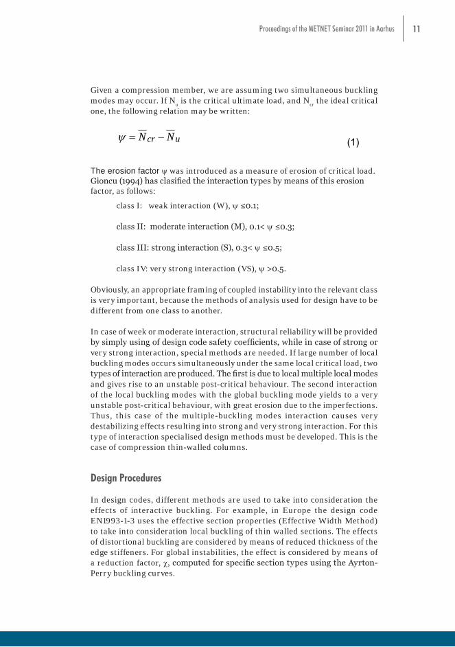
The general meaning of coupled instability phenomenon is related, in fact, to non-linear coupling. Due to the imperfections, an interaction erosion of critical bifurcation load occurs. This erosion is maximum in the coupling point vicinity. For bar members, an interactive slenderness range, in which sensitivity to imperfections is increased, may be identified. The erosion concept is depicted in Figure 3.
The instability behaviour of bar members is generally characterised by stable post-critical modes. However the interaction of two stable symmetric post-critical modes may generate an unstable coupled asymmetric mode, rendering the member highly sensitive to imperfections. In such case a significant erosion of critical load occurs. Interactive Buckling and the Erosion Concept The general meaning of coupled instability phenomenon is related, in fact, to non-linear coupling. Due to the imperfections, an interaction erosion of critical bifurcation load occurs. This erosion is maximum in the coupling point vicinity. For bar members, an interactive slenderness range, in which sensitivity to imperfections is increased, may be identified. The erosion concept is depicted in Figure 3.
Figure 3 – Erosion of Critical Bifurcation Load
Given a compression member, we are assuming two simultaneous buckling modes may occur. If Nu is the critical ultimate load, and Ncr the ideal critical one, the following relation may be written:
cr uN N (1)
The erosion factor was introduced as a measure of erosion of critical load. Gioncu (1994) has clasified the interaction types by means of this erosion factor, as follows:
class I: weak interaction (W), ≤0.1; class II: moderate interaction (M), 0.1< ≤0.3; class III: strong interaction (S), 0.3< ≤0.5; class IV: very strong interaction (VS), >0.5.
Obviously, an appropriate framing of coupled instability into the relevant class is very important, because the methods of analysis used for design have to be different from one class to another. In case of week or moderate interaction, structural reliability will be provided by simply using of design code safety coefficients, while in case of strong or very strong interaction, special methods are needed. If large number of local buckling modes occurs
Figure 3 – Erosion of Critical Bifurcation Load
11Proceedings of the METNET Seminar 2011 in Aarhus
Given a compression member, we are assuming two simultaneous buckling modes may occur. If N
u is the critical ultimate load, and N
cr the ideal critical
one, the following relation may be written:
The instability behaviour of bar members is generally characterised by stable post-critical modes. However the interaction of two stable symmetric post-critical modes may generate an unstable coupled asymmetric mode, rendering the member highly sensitive to imperfections. In such case a significant erosion of critical load occurs. Interactive Buckling and the Erosion Concept The general meaning of coupled instability phenomenon is related, in fact, to non-linear coupling. Due to the imperfections, an interaction erosion of critical bifurcation load occurs. This erosion is maximum in the coupling point vicinity. For bar members, an interactive slenderness range, in which sensitivity to imperfections is increased, may be identified. The erosion concept is depicted in Figure 3.
Figure 3 – Erosion of Critical Bifurcation Load
Given a compression member, we are assuming two simultaneous buckling modes may occur. If Nu is the critical ultimate load, and Ncr the ideal critical one, the following relation may be written:
cr uN N (1)
The erosion factor was introduced as a measure of erosion of critical load. Gioncu (1994) has clasified the interaction types by means of this erosion factor, as follows:
class I: weak interaction (W), ≤0.1; class II: moderate interaction (M), 0.1< ≤0.3; class III: strong interaction (S), 0.3< ≤0.5; class IV: very strong interaction (VS), >0.5.
Obviously, an appropriate framing of coupled instability into the relevant class is very important, because the methods of analysis used for design have to be different from one class to another. In case of week or moderate interaction, structural reliability will be provided by simply using of design code safety coefficients, while in case of strong or very strong interaction, special methods are needed. If large number of local buckling modes occurs
The erosion factor y was introduced as a measure of erosion of critical load. Gioncu (1994) has clasified the interaction types by means of this erosion factor, as follows:
class I: weak interaction (W), y ≤0.1;
class II: moderate interaction (M), 0.1< y ≤0.3;
class III: strong interaction (S), 0.3< y ≤0.5;
class IV: very strong interaction (VS), y >0.5.
Obviously, an appropriate framing of coupled instability into the relevant class is very important, because the methods of analysis used for design have to be different from one class to another.
In case of week or moderate interaction, structural reliability will be provided by simply using of design code safety coefficients, while in case of strong or very strong interaction, special methods are needed. If large number of local buckling modes occurs simultaneously under the same local critical load, two types of interaction are produced. The first is due to local multiple local modes and gives rise to an unstable post-critical behaviour. The second interaction of the local buckling modes with the global buckling mode yields to a very unstable post-critical behaviour, with great erosion due to the imperfections. Thus, this case of the multiple-buckling modes interaction causes very destabilizing effects resulting into strong and very strong interaction. For this type of interaction specialised design methods must be developed. This is the case of compression thin-walled columns.
Design Procedures
In design codes, different methods are used to take into consideration the effects of interactive buckling. For example, in Europe the design code EN1993-1-3 uses the effective section properties (Effective Width Method) to take into consideration local buckling of thin walled sections. The effects of distortional buckling are considered by means of reduced thickness of the edge stiffeners. For global instabilities, the effect is considered by means of a reduction factor, c, computed for specific section types using the Ayrton-Perry buckling curves.
12 Proceedings of the METNET Seminar 2011 in Aarhus
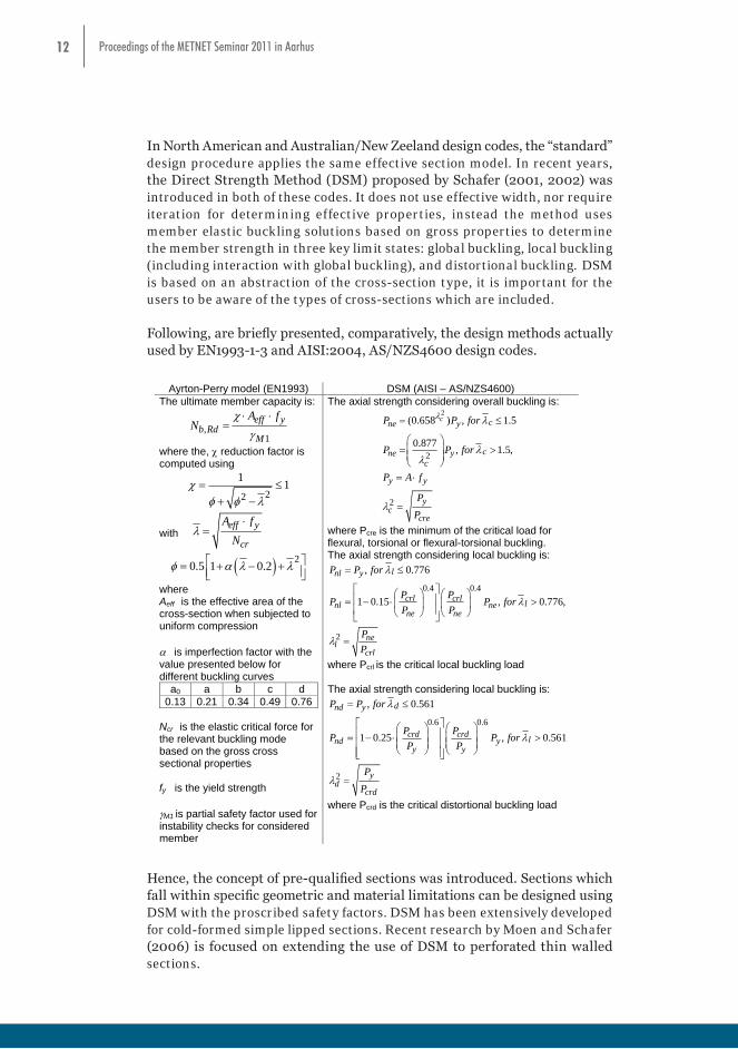
In North American and Australian/New Zeeland design codes, the “standard” design procedure applies the same effective section model. In recent years, the Direct Strength Method (DSM) proposed by Schafer (2001, 2002) was introduced in both of these codes. It does not use effective width, nor require iteration for determining effective properties, instead the method uses member elastic buckling solutions based on gross properties to determine the member strength in three key limit states: global buckling, local buckling (including interaction with global buckling), and distortional buckling. DSM is based on an abstraction of the cross-section type, it is important for the users to be aware of the types of cross-sections which are included.
Following, are briefly presented, comparatively, the design methods actually used by EN1993-1-3 and AISI:2004, AS/NZS4600 design codes.
Ayrton-Perry model (EN1993) DSM (AISI – AS/NZS4600) The ultimate member capacity is:
,1
eff yb Rd
M
A fN
where the, reduction factor is computed using
22
1 1
with eff y
cr
A fN
20.5 1 0.2 where Aeff is the effective area of the cross-section when subjected to uniform compression is imperfection factor with the value presented below for different buckling curves
a0 a b c d 0.13 0.21 0.34 0.49 0.76
Ncr is the elastic critical force for the relevant buckling mode based on the gross cross sectional properties
fy is the yield strength M1 is partial safety factor used for instability checks for considered member
The axial strength considering overall buckling is: 2
2
2
(0.658 )
0.877 ,
, 1.5
1.5,
cne c
c
y y
yc
y
ne yc
cre
for
for
P A f
P P
P
P
P
P
where Pcre is the minimum of the critical load for flexural, torsional or flexural-torsional buckling. The axial strength considering local buckling is:
0.4 4
2
0.
, 0.776
0.776. , ,1 0 15
nl y
crl crlnl ne
ne ne
l
l
nel
crl
P P
P PP PP P
for
for
PP
where Pcrl is the critical local buckling load
The axial strength considering local buckling is:
0.6 0 6
2
.
1 0.
, 0.561
0.565 12 ,
nd y
crd crdnd y
y y
d
l
yd
crd
P P
P PP PP
for
for
PP
P
where Pcrd is the critical distortional buckling load
Hence, the concept of pre-qualified sections was introduced. Sections which fall within specific geometric and material limitations can be designed using DSM with the proscribed safety factors. DSM has been extensively developed for cold-formed simple lipped sections. Recent research by Moen and Schafer (2006) is focused on extending the use of DSM to perforated thin walled sections.
Numerical Procedures
Hence, the concept of pre-qualified sections was introduced. Sections which fall within specific geometric and material limitations can be designed using DSM with the proscribed safety factors. DSM has been extensively developed for cold-formed simple lipped sections. Recent research by Moen and Schafer (2006) is focused on extending the use of DSM to perforated thin walled sections.
13Proceedings of the METNET Seminar 2011 in Aarhus
Numerical Procedures
Various numerical tools are currently used nowadays by engineers in the design to provide the ultimate or critical forces for specific instabilities. Finite Element Method (FEM), Finite Strip Method (FSM) and Generalised Beam Theory (GBT) are the most versatile approaches to consider simple and coupled instabilities of thin walled sections.
Each one of these methods has its advantages and disadvantages.
The FEM is a numerical approach that allows the analysis of a numerical model representing the real structure (or a component) within the computer software. The advantages of FEM are summarized below:
• loads can be placed in any point on the member and in any direction,
• the analysis solvers can incorporate non-linear stress-strain relationship and non-linear geometry
• point-contact elements, links, and/or compression only members can be used to model the contact between connected components
• perforations and complex boundary conditions can be included if required.
The main disadvantage of FEM is that it requires a large amount of computational time in comparison with FSM and GBT. When studying thin walled sections, it is difficult to apply directly modal decomposition for these sections, this fact constituting another major disadvantage of FEM.
On the other hand FSM is a semi-analytical semi-numerical approach based on half sine wave displacement functions that offers modal decomposition by imposing constraints in order to control nodal relative displacement. It requires less time to build a model and requires less memory and consequently less time to run. The specific version of the finite strip method which could account for both plate flexural buckling and membrane buckling in thin-walled members was developed by Plank and Wittrick (1974). Lau extended the finite strip buckling capabilities to the spline finite strip method to allow for fixed-ended boundary conditions, performed experiments in which distortional buckling was the failure mechanism (Lau and Hancock, 1990). The major limitation of this method concerns the loads applications (only axial load or bending moment that gives constant stress distribution can be applied).
When discussing about instabilities, GBT offers many advantages. It is an extension to conventional engineering beam theory that allows cross-section distortion to be considered in the stability analysis of thin-walled members. GBT may be viewed as either (i) a bar theory incorporating cross-section in and out-of-plane deformations or (ii) a folded plate theory that includes plate
14 Proceedings of the METNET Seminar 2011 in Aarhus
rigid-body motions (Camotim et al. 2004). By decomposing the member deformed configurations or buckling/vibration mode shapes into linear combinations of longitudinally varying cross-section deformation modes, GBT provides a general and elegant approach to obtain accurate solutions for several structural problems involving prismatic thin-walled members − moreover, one also obtains the contributions of each deformation mode, a feature enabling a much clearer interpretation of the structural response under consideration.
By decomposing the member buckling modes into linear combinations of “pure deformation modes”, GBT offers possibilities not available even through the use of powerful numerical techniques (FEM or FSM) and provides a general and elegant approach to obtain accurate solutions for several stability problems. Moreover, it is possible (i) to consider different types of loading, (ii) to take into account the presence of arbitrary initial geometrical imperfections and (iii) to determine, with great accuracy, “exact” and “approximate” (i.e. including just a few deformation modes) member post-buckling equilibrium paths.
Erosion of critical bifuraction load – ECBL approach
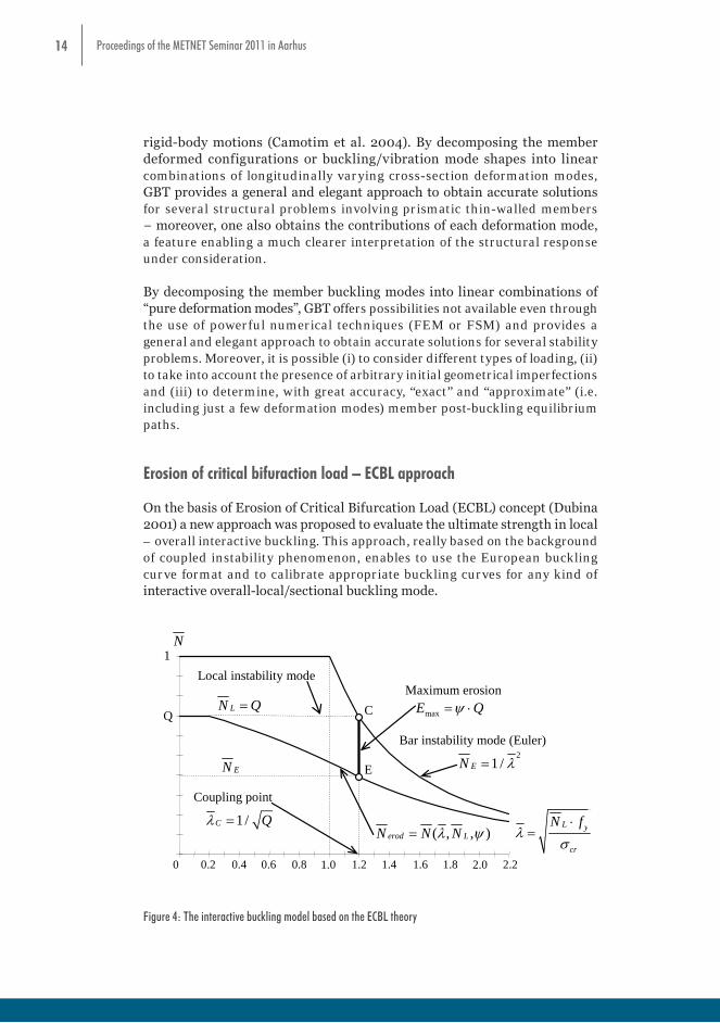
On the basis of Erosion of Critical Bifurcation Load (ECBL) concept (Dubina 2001) a new approach was proposed to evaluate the ultimate strength in local – overall interactive buckling. This approach, really based on the background of coupled instability phenomenon, enables to use the European buckling curve format and to calibrate appropriate buckling curves for any kind of interactive overall-local/sectional buckling mode.
0 0.2 0.4 0.6 0.8 1.0 1.2 1.4 1.6 1.8 2.0 2.2
Local instability mode Maximum erosion
Coupling point
Bar instability mode (Euler)
CQ
1
E2
1 /EN
N
LN Q
EN
maxE Q
1/C Q ( , , )erod LN N N
L y
cr
N f
Figure 4: The interactive buckling model based on the ECBL theory
Assuming the two theoretical simple instability modes that couple in a thin-walled compression member, are the Euler bar instability mode, 2
1 /EN (e.g. can be the flexural, F , or flexural-torsional, FT , slenderness) and the local instability mode,
/L effN A A Q (see Figure 4), then the maximum erosion of critical load, due both, to the
imperfections and coupling effect occurs in the coupling point 1/C LN .
The interactive buckling load, ( , , )LN N , pass through this point and the corresponding value of ultimate buckling load is , (1 )erod E LN N , where is the erosion factor.
It must be underlined that LN does not represent rigorously the theoretical local buckling curve, but it can be assumed, being the lower bound of the sectional strength as a reference or a practical strength of the cross-section corresponding to the local buckling mode. On the basis of this assumption, it is possibly to evaluate the ultimate strength of the stub column. One might call the coupling point C, obtained according to this mode, the practical interaction point. Similarly, the same approach can be applied for the case where the interaction occurs between the distortional mode, /D D plN N N , pl yN A f , and overall mode.
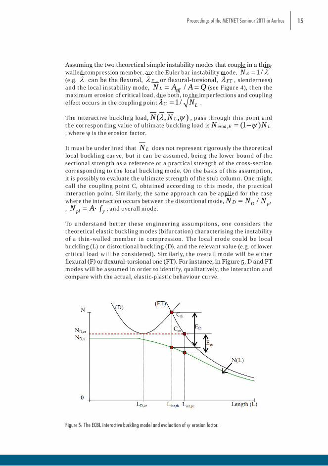
To understand better these engineering assumptions, one considers the theoretical elastic buckling modes (bifurcation) characterising the instability of a thin-walled member in compression. The local mode could be local buckling (L) or distortional buckling (D), and the relevant value (e.g. of lower critical load will be considered). Similarly, the overall mode will be either flexural (F) or flexural-torsional one (FT). For instance, in Figure 5, D and FT modes will be assumed in order to identify, qualitatively, the interaction and compare with the actual, elastic-plastic behaviour curve.
Figure 4: The interactive buckling model based on the ECBL theory
15Proceedings of the METNET Seminar 2011 in Aarhus
Assuming the two theoretical simple instability modes that couple in a thin-walled compression member, are the Euler bar instability mode,
21 /EN λ=
(e.g. λ can be the flexural, Fλ , or flexural-torsional, FTλ , slenderness) and the local instability mode, /L effN A A Q= = (see Figure 4), then the maximum erosion of critical load, due both, to the imperfections and coupling effect occurs in the coupling point 1/C LNλ = .
The interactive buckling load, ( , , )LN Nλ y , pass through this point and the corresponding value of ultimate buckling load is , (1 )erod E LN Ny= -, where y is the erosion factor.
It must be underlined that LN does not represent rigorously the theoretical local buckling curve, but it can be assumed, being the lower bound of the sectional strength as a reference or a practical strength of the cross-section corresponding to the local buckling mode. On the basis of this assumption, it is possibly to evaluate the ultimate strength of the stub column. One might call the coupling point C, obtained according to this mode, the practical interaction point. Similarly, the same approach can be applied for the case where the interaction occurs between the distortional mode, /D D plN N N=, pl yN A f= ⋅ , and overall mode.
To understand better these engineering assumptions, one considers the theoretical elastic buckling modes (bifurcation) characterising the instability of a thin-walled member in compression. The local mode could be local buckling (L) or distortional buckling (D), and the relevant value (e.g. of lower critical load will be considered). Similarly, the overall mode will be either flexural (F) or flexural-torsional one (FT). For instance, in Figure 5, D and FT modes will be assumed in order to identify, qualitatively, the interaction and compare with the actual, elastic-plastic behaviour curve.
Figure 5: The ECBL interactive buckling model and evaluation of erosion factor.
Modes (D) and (FT) are interacting into the theoretical coupling point Cth, while mode N=ND,cr with (FT) into practical coupling point Cpr. Correspondingly to the two coupling points and related to the actual elastic-plastic N(L) curve will be the theoretical, Eth, and practical, Epr, erosions.
The use of practical interaction has the advantage to give the possibility to use Ayrton-Perry model and the European buckling curve format in order to obtain interactive buckling curves as it will be shown in the following. The Ayrton-Perry equation can be written in the form:
2(1 ) 1 ( 0.2)N N N
(1)
It is easy to show the relation between the imperfection and erosion factor. The negative sign solution of equation (1), in the particular point 1 has to be taken equal with 1 ,because it corresponds to the maximum erosion of the Euler curve when no local buckling occurs. In this case the erosion can be associated to the plastic-elastic interaction between the rigid plastic mode (plastic strength) of stub column and the overall elastic buckling mode of the bar, given by Euler formula. When distortional buckling occurs prior to bar buckling, the corresponding solution of equation
2( )(1 ) ( 0.2)DN N N N , in the
coupling point, E is 2
2 222 2
1 ( 0.2) 1 [1 ( 0.2) ] 4 (1 )2 2
DD D D
NN N N N
(2)
which leads to 2
1 1 0 .2D
D
N
N
(3)
Equation (3) represents the new formula of imperfection coefficient which should be introduced in European buckling curves in order to adapt these curves to distortional-overall interactive buckling.
There are three distinct approaches that can be used to evaluate the erosion factor: (i) the analytical approach, having as main goal to compute the decrease of axial rigidity of the related column in the vicinity of critical bifurcation point, (ii) the numerical approach
Figure 5: The ECBL interactive buckling model and evaluation of y erosion factor.

16 Proceedings of the METNET Seminar 2011 in Aarhus
Modes (D) and (FT) are interacting into the theoretical coupling point Cth
, while mode N=N
D,cr
with (FT) into practical coupling point Cpr
. Correspondingly to the two coupling points and related to the actual elastic-plastic N(L) curve will be the theoretical, E
th, and practical, E
pr, erosions.
The use of practical interaction has the advantage to give the possibility to use Ayrton-Perry model and the European buckling curve format in order to obtain interactive buckling curves as it will be shown in the following. The Ayrton-Perry equation can be written in the form:
Figure 5: The ECBL interactive buckling model and evaluation of erosion factor.
Modes (D) and (FT) are interacting into the theoretical coupling point Cth, while mode N=ND,cr with (FT) into practical coupling point Cpr. Correspondingly to the two coupling points and related to the actual elastic-plastic N(L) curve will be the theoretical, Eth, and practical, Epr, erosions.
The use of practical interaction has the advantage to give the possibility to use Ayrton-Perry model and the European buckling curve format in order to obtain interactive buckling curves as it will be shown in the following. The Ayrton-Perry equation can be written in the form:
2(1 ) 1 ( 0.2)N N N
(1)
It is easy to show the relation between the imperfection and erosion factor. The negative sign solution of equation (1), in the particular point 1 has to be taken equal with 1 ,because it corresponds to the maximum erosion of the Euler curve when no local buckling occurs. In this case the erosion can be associated to the plastic-elastic interaction between the rigid plastic mode (plastic strength) of stub column and the overall elastic buckling mode of the bar, given by Euler formula. When distortional buckling occurs prior to bar buckling, the corresponding solution of equation
2( )(1 ) ( 0.2)DN N N N , in the
coupling point, E is 2
2 222 2
1 ( 0.2) 1 [1 ( 0.2) ] 4 (1 )2 2
DD D D
NN N N N
(2)
which leads to 2
1 1 0 .2D
D
N
N
(3)
Equation (3) represents the new formula of imperfection coefficient which should be introduced in European buckling curves in order to adapt these curves to distortional-overall interactive buckling.
There are three distinct approaches that can be used to evaluate the erosion factor: (i) the analytical approach, having as main goal to compute the decrease of axial rigidity of the related column in the vicinity of critical bifurcation point, (ii) the numerical approach
It is easy to show the relation between the imperfection and erosion factor. The negative sign solution of equation (1), in the particular point 1λ = has to be taken equal with ( )1 y- , because it corresponds to the maximum erosion of the Euler curve when no local buckling occurs. In this case the erosion can be associated to the plastic-elastic interaction between the rigid plastic mode (plastic strength) of stub column and the overall elastic buckling mode of the bar, given by Euler formula. When distortional buckling occurs prior to bar buckling, the corresponding solution of equation
2( )(1 ) ( 0.2)DN N N Nλ a λ- - = - , in the coupling point, E is
Figure 5: The ECBL interactive buckling model and evaluation of erosion factor.
Modes (D) and (FT) are interacting into the theoretical coupling point Cth, while mode N=ND,cr with (FT) into practical coupling point Cpr. Correspondingly to the two coupling points and related to the actual elastic-plastic N(L) curve will be the theoretical, Eth, and practical, Epr, erosions.
The use of practical interaction has the advantage to give the possibility to use Ayrton-Perry model and the European buckling curve format in order to obtain interactive buckling curves as it will be shown in the following. The Ayrton-Perry equation can be written in the form:
2(1 ) 1 ( 0.2)N N N
(1)
It is easy to show the relation between the imperfection and erosion factor. The negative sign solution of equation (1), in the particular point 1 has to be taken equal with 1 ,because it corresponds to the maximum erosion of the Euler curve when no local buckling occurs. In this case the erosion can be associated to the plastic-elastic interaction between the rigid plastic mode (plastic strength) of stub column and the overall elastic buckling mode of the bar, given by Euler formula. When distortional buckling occurs prior to bar buckling, the corresponding solution of equation
2( )(1 ) ( 0.2)DN N N N , in the
coupling point, E is 2
2 222 2
1 ( 0.2) 1 [1 ( 0.2) ] 4 (1 )2 2
DD D D
NN N N N
(2)
which leads to 2
1 1 0 .2D
D
N
N
(3)
Equation (3) represents the new formula of imperfection coefficient which should be introduced in European buckling curves in order to adapt these curves to distortional-overall interactive buckling.
There are three distinct approaches that can be used to evaluate the erosion factor: (i) the analytical approach, having as main goal to compute the decrease of axial rigidity of the related column in the vicinity of critical bifurcation point, (ii) the numerical approach
which leads to
Figure 5: The ECBL interactive buckling model and evaluation of erosion factor.
Modes (D) and (FT) are interacting into the theoretical coupling point Cth, while mode N=ND,cr with (FT) into practical coupling point Cpr. Correspondingly to the two coupling points and related to the actual elastic-plastic N(L) curve will be the theoretical, Eth, and practical, Epr, erosions.
The use of practical interaction has the advantage to give the possibility to use Ayrton-Perry model and the European buckling curve format in order to obtain interactive buckling curves as it will be shown in the following. The Ayrton-Perry equation can be written in the form:
2(1 ) 1 ( 0.2)N N N
(1)
It is easy to show the relation between the imperfection and erosion factor. The negative sign solution of equation (1), in the particular point 1 has to be taken equal with 1 ,because it corresponds to the maximum erosion of the Euler curve when no local buckling occurs. In this case the erosion can be associated to the plastic-elastic interaction between the rigid plastic mode (plastic strength) of stub column and the overall elastic buckling mode of the bar, given by Euler formula. When distortional buckling occurs prior to bar buckling, the corresponding solution of equation
2( )(1 ) ( 0.2)DN N N N , in the
coupling point, E is 2
2 222 2
1 ( 0.2) 1 [1 ( 0.2) ] 4 (1 )2 2
DD D D
NN N N N
(2)
which leads to 2
1 1 0 .2D
D
N
N
(3)
Equation (3) represents the new formula of imperfection coefficient which should be introduced in European buckling curves in order to adapt these curves to distortional-overall interactive buckling.
There are three distinct approaches that can be used to evaluate the erosion factor: (i) the analytical approach, having as main goal to compute the decrease of axial rigidity of the related column in the vicinity of critical bifurcation point, (ii) the numerical approach
Equation (3) represents the new formula of a imperfection coefficient which should be introduced in European buckling curves in order to adapt these curves to distortional-overall interactive buckling.
There are three distinct approaches that can be used to evaluate the y erosion factor: (i) the analytical approach, having as main goal to compute the decrease of axial rigidity of the related column in the vicinity of critical bifurcation point, (ii) the numerical approach based on Finite Element (FE) non-linear analysis of the behavior of thin-walled columns in the vicinity of critical bifurcation point and (iii) the experimental approach by means of statistical analysis of some representative series of column test results corresponding to specified cross-section shape, characterized by means of Q
D factor.
17Proceedings of the METNET Seminar 2011 in Aarhus
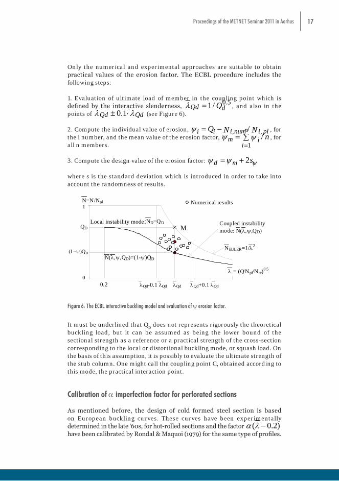
Only the numerical and experimental approaches are suitable to obtain practical values of the erosion factor. The ECBL procedure includes the following steps:
1. Evaluation of ultimate load of member in the coupling point which is defined by the interactive slenderness,
0.51/Qd dQλ = , and also in the points of 0.1Qd Qdλ λ± ⋅ (see Figure 6).
2. Compute the individual value of erosion, , ,/i num i pli iQ N Ny = - , for the i number, and the mean value of the erosion factor,
1/
nm i
iny y
== ∑ , for
all n members.
3. Compute the design value of the erosion factor: 2d m syy y= +
where s is the standard deviation which is introduced in order to take into account the randomness of results.
based on Finite Element (FE) non-linear analysis of the behavior of thin-walled columns in the vicinity of critical bifurcation point and (iii) the experimental approach by means of statistical analysis of some representative series of column test results corresponding to specified cross-section shape, characterized by means of QD factor.
Only the numerical and experimental approaches are suitable to obtain practical values of the erosion factor. The ECBL procedure includes the following steps: 1. Evaluation of ultimate load of member in the coupling point which is defined by the interactive slenderness, 0.51/Qd dQ , and also in the points of 0.1Qd Qd (see Figure 6). 2. Compute the individual value of erosion, , ,/i num i pli iQ N N , for the i number, and
the mean value of the erosion factor, 1
/n
m ii
n
, for all n members.
3. Compute the design value of the erosion factor: 2d m s
where s is the standard deviation which is introduced in order to take into account the randomness of results.
0
1N=N/Npl
= (Q.Npl/Ncr)0.5
QDNEULER=1/2
QDLocal instability mode:ND=QD
M
QdQd-0.1 Qd Qd+0.1 Qd
N(,QD)=(1-)QD
0.2
Coupled instability mode: N(,QD)
Numerical results
Figure 6: The ECBL interactive buckling model and evaluation of erosion factor.
It must be underlined that QD does not represents rigorously the theoretical buckling load, but it can be assumed as being the lower bound of the sectional strength as a reference or a practical strength of the cross-section corresponding to the local or distortional buckling mode, or squash load. On the basis of this assumption, it is possibly to evaluate the ultimate strength of the stub column. One might call the coupling point C, obtained according to this mode, the practical interaction point.
Calibration of imperfection factor for perforated sections
As mentioned before, the design of cold formed steel section is based on European buckling curves. These curves have been experimentally determined in the late ‘60s, for hot-rolled sections and the factor ( 0.2) have been calibrated by Rondal & Maquoi (1979) for the same type of profiles. It is not normal to use the values of imperfection factors calibrated for hot-rolled profiles in the design of thin walled sections.
Figure 6: The ECBL interactive buckling model and evaluation of y erosion factor.
It must be underlined that QD does not represents rigorously the theoretical
buckling load, but it can be assumed as being the lower bound of the sectional strength as a reference or a practical strength of the cross-section corresponding to the local or distortional buckling mode, or squash load. On the basis of this assumption, it is possibly to evaluate the ultimate strength of the stub column. One might call the coupling point C, obtained according to this mode, the practical interaction point.
Calibration of a imperfection factor for perforated sections
As mentioned before, the design of cold formed steel section is based on European buckling curves. These curves have been experimentally determined in the late ‘60s, for hot-rolled sections and the factor ( 0.2)a λ - have been calibrated by Rondal & Maquoi (1979) for the same type of profiles.
18 Proceedings of the METNET Seminar 2011 in Aarhus
It is not normal to use the values of a imperfection factors calibrated for hot-rolled profiles in the design of thin walled sections.
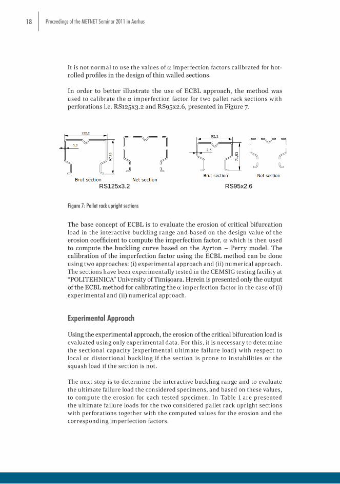
In order to better illustrate the use of ECBL approach, the method was used to calibrate the a imperfection factor for two pallet rack sections with perforations i.e. RS125x3.2 and RS95x2.6, presented in Figure 7.In order to better illustrate the use of ECBL approach, the method was used to calibrate
the imperfection factor for two pallet rack sections with perforations i.e. RS125x3.2 and RS95x2.6, presented in Figure 7.
RS125x3.2 RS95x2.6
Figure 7: Pallet rack upright sections The base concept of ECBL is to evaluate the erosion of critical bifurcation load in the interactive buckling range and based on the design value of the erosion coefficient to compute the imperfection factor, which is then used to compute the buckling curve based on the Ayrton – Perry model. The calibration of the imperfection factor using the ECBL method can be done using two approaches: (i) experimental approach and (ii) numerical approach. The sections have been experimentally tested in the CEMSIG testing facility at “POLITEHNICA” University of Timişoara. Herein is presented only the output of the ECBL method for calibrating the imperfection factor in the case of (i) experimental and (ii) numerical approach. Experimental Approach Using the experimental approach, the erosion of the critical bifurcation load is evaluated using only experimental data. For this, it is necessary to determine the sectional capacity (experimental ultimate failure load) with respect to local or distortional buckling if the section is prone to instabilities or the squash load if the section is not. The next step is to determine the interactive buckling range and to evaluate the ultimate failure load the considered specimens, and based on these values, to compute the erosion for each tested specimen. In Table 1 are presented the ultimate failure loads for the two considered pallet rack upright sections with perforations together with the computed values for the erosion and the corresponding imperfection factors.
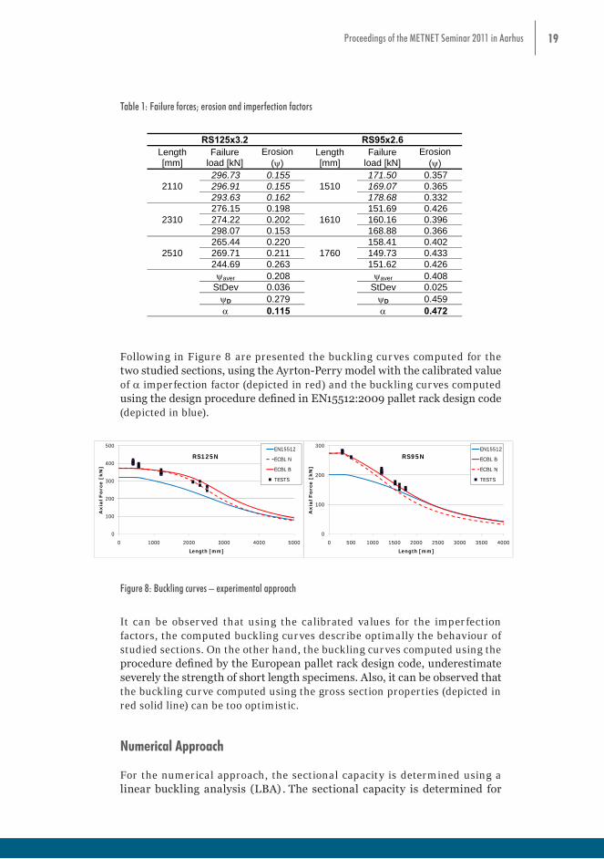
Table 1: Failure forces; erosion and imperfection factors RS125x3.2 RS95x2.6
Length [mm]
Failure load [kN]
Erosion ()
Length [mm]
Failure load [kN]
Erosion ()
2110 296.73 0.155
1510 171.50 0.357
296.91 0.155 169.07 0.365 293.63 0.162 178.68 0.332
2310 276.15 0.198
1610 151.69 0.426
274.22 0.202 160.16 0.396 298.07 0.153 168.88 0.366
2510 265.44 0.220 1760 158.41 0.402 269.71 0.211 149.73 0.433
Figure 7: Pallet rack upright sections
The base concept of ECBL is to evaluate the erosion of critical bifurcation load in the interactive buckling range and based on the design value of the erosion coefficient to compute the imperfection factor, a which is then used to compute the buckling curve based on the Ayrton – Perry model. The calibration of the imperfection factor using the ECBL method can be done using two approaches: (i) experimental approach and (ii) numerical approach. The sections have been experimentally tested in the CEMSIG testing facility at “POLITEHNICA” University of Timişoara. Herein is presented only the output of the ECBL method for calibrating the a imperfection factor in the case of (i) experimental and (ii) numerical approach.
Experimental Approach
Using the experimental approach, the erosion of the critical bifurcation load is evaluated using only experimental data. For this, it is necessary to determine the sectional capacity (experimental ultimate failure load) with respect to local or distortional buckling if the section is prone to instabilities or the squash load if the section is not.
The next step is to determine the interactive buckling range and to evaluate the ultimate failure load the considered specimens, and based on these values, to compute the erosion for each tested specimen. In Table 1 are presented the ultimate failure loads for the two considered pallet rack upright sections with perforations together with the computed values for the erosion and the corresponding imperfection factors.
19Proceedings of the METNET Seminar 2011 in Aarhus
Table 1: Failure forces; erosion and imperfection factors
RS125x3.2 RS95x2.6 Length [mm]
Failure load [kN]
Erosion ()
Length [mm]
Failure load [kN]
Erosion ()
2110 296.73 0.155
1510 171.50 0.357
296.91 0.155 169.07 0.365 293.63 0.162 178.68 0.332
2310 276.15 0.198
1610 151.69 0.426
274.22 0.202 160.16 0.396 298.07 0.153 168.88 0.366
2510 265.44 0.220
1760 158.41 0.402
269.71 0.211 149.73 0.433 244.69 0.263 151.62 0.426 aver 0.208 aver 0.408
StDev 0.036 StDev 0.025 D 0.279 D 0.459 0.115 0.472
Following in Figure 8 are presented the buckling curves computed for the two studied sections, using the Ayrton-Perry model with the calibrated value of imperfection factor (depicted in red) and the buckling curves computed using the design procedure defined in EN15512:2009 pallet rack design code (depicted in blue).
0
100
200
300
400
500
0 1000 2000 3000 4000 5000
Axia
l Fo
rce [
kN
]
Length [mm]
RS125NEN15512
ECBL N
ECBL B
TESTS
0
100
200
300
0 500 1000 1500 2000 2500 3000 3500 4000
Axia
l Fo
rce [
kN
]
Length [mm]
RS95NEN15512
ECBL B
ECBL N
TESTS
Figure 8: Buckling curves – experimental approach
It can be observed that using the calibrated values for the imperfection factors, the computed buckling curves describe optimally the behaviour of studied sections. On the other hand, the buckling curves computed using the procedure defined by the European pallet rack design code, underestimate severely the strength of short length specimens. Also, it can be observed that the buckling curve computed using the gross section properties (depicted in red solid line) can be too optimistic.
Numerical Approach
For the numerical approach, the sectional capacity is determined using a linear buckling analysis (LBA). The sectional capacity is determined for the considered buckling mode i.e. local or distortional and taken to be the minimum critical buckling load for the two considered sectional instabilities. If the section is not prone to sectional buckling, the sectional capacity is considered to be equal with the squash load.
Following in Figure 8 are presented the buckling curves computed for the two studied sections, using the Ayrton-Perry model with the calibrated value of a imperfection factor (depicted in red) and the buckling curves computed using the design procedure defined in EN15512:2009 pallet rack design code (depicted in blue).
RS125x3.2 RS95x2.6 Length [mm]
Failure load [kN]
Erosion ()
Length [mm]
Failure load [kN]
Erosion ()
2110 296.73 0.155
1510 171.50 0.357
296.91 0.155 169.07 0.365 293.63 0.162 178.68 0.332
2310 276.15 0.198
1610 151.69 0.426
274.22 0.202 160.16 0.396 298.07 0.153 168.88 0.366
2510 265.44 0.220
1760 158.41 0.402
269.71 0.211 149.73 0.433 244.69 0.263 151.62 0.426 aver 0.208 aver 0.408
StDev 0.036 StDev 0.025 D 0.279 D 0.459 0.115 0.472
Following in Figure 8 are presented the buckling curves computed for the two studied sections, using the Ayrton-Perry model with the calibrated value of imperfection factor (depicted in red) and the buckling curves computed using the design procedure defined in EN15512:2009 pallet rack design code (depicted in blue).
0
100
200
300
400
500
0 1000 2000 3000 4000 5000
Axia
l Fo
rce [
kN
]
Length [mm]
RS125NEN15512
ECBL N
ECBL B
TESTS
0
100
200
300
0 500 1000 1500 2000 2500 3000 3500 4000
Axia
l Fo
rce [
kN
]
Length [mm]
RS95NEN15512
ECBL B
ECBL N
TESTS
Figure 8: Buckling curves – experimental approach
It can be observed that using the calibrated values for the imperfection factors, the computed buckling curves describe optimally the behaviour of studied sections. On the other hand, the buckling curves computed using the procedure defined by the European pallet rack design code, underestimate severely the strength of short length specimens. Also, it can be observed that the buckling curve computed using the gross section properties (depicted in red solid line) can be too optimistic.
Numerical Approach
For the numerical approach, the sectional capacity is determined using a linear buckling analysis (LBA). The sectional capacity is determined for the considered buckling mode i.e. local or distortional and taken to be the minimum critical buckling load for the two considered sectional instabilities. If the section is not prone to sectional buckling, the sectional capacity is considered to be equal with the squash load.
Figure 8: Buckling curves – experimental approach
It can be observed that using the calibrated values for the imperfection factors, the computed buckling curves describe optimally the behaviour of studied sections. On the other hand, the buckling curves computed using the procedure defined by the European pallet rack design code, underestimate severely the strength of short length specimens. Also, it can be observed that the buckling curve computed using the gross section properties (depicted in red solid line) can be too optimistic.
Numerical Approach
For the numerical approach, the sectional capacity is determined using a linear buckling analysis (LBA) . The sectional capacity is determined for

20 Proceedings of the METNET Seminar 2011 in Aarhus
the considered buckling mode i.e. local or distortional and taken to be the minimum critical buckling load for the two considered sectional instabilities. If the section is not prone to sectional buckling, the sectional capacity is considered to be equal with the squash load.
The evaluation of erosion is based on an imperfection sensitivity study conducted using a numerical model calibrated against experimental tests. For the case of the two studied sections, the imperfection sensitivity study was conducted using the coded values for sectional imperfections (type 2 imperfection as defined by Schafer & Pekoz, 1998) (d
2=t) and an initial
bow imperfection in accordance with the specifications of EN 1090-2:2008 ( f=L/750) as the maximum allowed manufacturing tolerance.
In Figure 9 is presented the considered set of imperfections for the numerical analysis of the thin walled section.
Figure 9: Example of considered initial imperfection
The obtained values for the calibrated a imperfection factor are presented in Table 2, together with the sectional capacity for the two considered sections.
Table 2: Sectional capacity and imperfection factors
RS125x3.2 RS95x2.6 Sectional
capacity [kN] Imperfection
factorSectional
capacity [kN] Imperfection
factor370.48 0.273 286.69 0.639
For RS125x3.2 section the sectional capacity is dictated by the distortional buckling capacity (distortional critical buckling load), while for RS95x2.6 the sectional capacity is equal with the squash load, since the section is not prone to sectional instabilities.
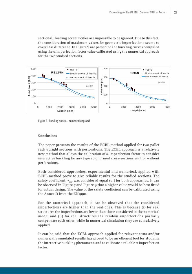
It must be specified that the measured imperfections for studied sections were found to be less than the before mentioned values. On the other hand, for experimental testing, together with geometric imperfections (global and/or sectional), loading eccentricities are impossible to be ignored. Due to this fact, the consideration of maximum values for geometric imperfections seems to cover this difference. In Figure 9 are presented the buckling curves computed using the imperfection factor value calibrated using the numerical approach for the two studied sections.
500
0
100
200
300
400
500
0 1000 2000 3000 4000 5000
Axia
l Lo
ad
[kN
]
Length [mm]
RS125NTESTS
Brut moment of inertia
Net moment of inertia
400
0
100
200
300
400
0 1000 2000 3000 4000
Axia
l lo
ad
[kN
]
Length [mm]
RS95NTESTS
Brut moment of inertia
Net moment of inertia
Figure 9: Buckling curves – numerical approach
Conclusions
Figure 9: Example of considered initial imperfection
The obtained values for the calibrated a imperfection factor are presented in Table 2, together with the sectional capacity for the two considered sections.
Table 2: Sectional capacity and imperfection factors
Figure 9: Example of considered initial imperfection
The obtained values for the calibrated a imperfection factor are presented in Table 2, together with the sectional capacity for the two considered sections.
Table 2: Sectional capacity and imperfection factors
RS125x3.2 RS95x2.6 Sectional
capacity [kN] Imperfection
factorSectional
capacity [kN] Imperfection
factor370.48 0.273 286.69 0.639
For RS125x3.2 section the sectional capacity is dictated by the distortional buckling capacity (distortional critical buckling load), while for RS95x2.6 the sectional capacity is equal with the squash load, since the section is not prone to sectional instabilities.
It must be specified that the measured imperfections for studied sections were found to be less than the before mentioned values. On the other hand, for experimental testing, together with geometric imperfections (global and/or sectional), loading eccentricities are impossible to be ignored. Due to this fact, the consideration of maximum values for geometric imperfections seems to cover this difference. In Figure 9 are presented the buckling curves computed using the imperfection factor value calibrated using the numerical approach for the two studied sections.
500
0
100
200
300
400
500
0 1000 2000 3000 4000 5000
Axia
l Lo
ad
[kN
]
Length [mm]
RS125NTESTS
Brut moment of inertia
Net moment of inertia
400
0
100
200
300
400
0 1000 2000 3000 4000
Axia
l lo
ad
[kN
]
Length [mm]
RS95NTESTS
Brut moment of inertia
Net moment of inertia
Figure 9: Buckling curves – numerical approach
Conclusions
For RS125x3.2 section the sectional capacity is dictated by the distortional buckling capacity (distortional critical buckling load), while for RS95x2.6 the sectional capacity is equal with the squash load, since the section is not prone to sectional instabilities.
It must be specified that the measured imperfections for studied sections were found to be less than the before mentioned values. On the other hand, for experimental testing, together with geometric imperfections (global and/or
21Proceedings of the METNET Seminar 2011 in Aarhus
sectional), loading eccentricities are impossible to be ignored. Due to this fact, the consideration of maximum values for geometric imperfections seems to cover this difference. In Figure 9 are presented the buckling curves computed using the a imperfection factor value calibrated using the numerical approach for the two studied sections.
Figure 9: Example of considered initial imperfection
The obtained values for the calibrated a imperfection factor are presented in Table 2, together with the sectional capacity for the two considered sections.
Table 2: Sectional capacity and imperfection factors
RS125x3.2 RS95x2.6 Sectional
capacity [kN] Imperfection
factorSectional
capacity [kN] Imperfection
factor370.48 0.273 286.69 0.639
For RS125x3.2 section the sectional capacity is dictated by the distortional buckling capacity (distortional critical buckling load), while for RS95x2.6 the sectional capacity is equal with the squash load, since the section is not prone to sectional instabilities.
It must be specified that the measured imperfections for studied sections were found to be less than the before mentioned values. On the other hand, for experimental testing, together with geometric imperfections (global and/or sectional), loading eccentricities are impossible to be ignored. Due to this fact, the consideration of maximum values for geometric imperfections seems to cover this difference. In Figure 9 are presented the buckling curves computed using the imperfection factor value calibrated using the numerical approach for the two studied sections.
500
0
100
200
300
400
500
0 1000 2000 3000 4000 5000
Axia
l Lo
ad
[kN
]
Length [mm]
RS125NTESTS
Brut moment of inertia
Net moment of inertia
400
0
100
200
300
400
0 1000 2000 3000 4000
Axia
l lo
ad
[kN
]
Length [mm]
RS95NTESTS
Brut moment of inertia
Net moment of inertia
Figure 9: Buckling curves – numerical approach
Conclusions
Figure 9: Buckling curves – numerical approach
Conclusions
The paper presents the results of the ECBL method applied for two pallet rack upright sections with perforations. The ECBL approach is a relatively new method that allows the calibration of a imperfection factor to consider interactive buckling for any type cold formed cross-sections with or without perforations.
Both considered approaches, experimental and numerical, applied with ECBL method prove to give reliable results for the studied sections. The safety coefficient, g
M1, was considered equal to 1 for both approaches. It can
be observed in Figure 7 and Figure 9 that a higher value would be best fitted for actual design. The value of the safety coefficient can be calibrated using the Annex D from the EN1990.
For the numerical approach, it can be observed that the considered imperfections are higher than the real ones. This is because (i) for real structures the imperfections are lower than those considered in the numerical model and (ii) for real structures the random imperfections partially compensate each other, while in numerical simulation they are cumulatively applied.
It can be said that the ECBL approach applied for relevant tests and/or numerically simulated results has proved to be an efficient tool for studying the interactive buckling phenomena and to calibrate a reliable a imperfection factor.

22 Proceedings of the METNET Seminar 2011 in Aarhus
References
Camotim D., Silvestre N., Gonçalves R. and Dinis P.B. (2004), “GBT analysis of thin-walled members: new formulations and applications”, Thin-Walled Structures: Recent Advances and Future Trends in Thin-Walled Structures Technology (Loughborough, 25/6), J. Loughlan (ed.), Canopus Publishing, Bath, 137-168,
Dubina D. (1996), “Coupled instabilities in bar members – General Report. Coupled Instabilities in Metal Structures” – CISM‟96 (Rondal J, Dubina D & Gioncu V, Eds.). Imperial College Press, London, p. 119-132
Dubina, D. (2001), ”The ECBL approach for interactive buckling of thin-walled steel members”, Steel & Composite Structures, 1,p. 75-96
Gioncu, V. (1994). General Theory of Coupled Instabilities - General Report. Thin-Walled Structures, 19(1-4), p. 81-127
Hancock G.J. (1998) “Design of Cold-formed Steel Structures, 3rd edition,” Australian Institute of Steel Construction, Sydney
Hancock, G.J. (1985). “Distortional Buckling of Steel Storage Rack Columns”. Journal of Structural Eng., ASCE, 111(12), pp. 2770-2783.
Lau, S.C.W. and Hancock, G.J (1990).,”Inelastic Buckling of Channel Columns in the Distortional Mode”, Thin-Walled Structures, 10(1), pp. 59-84.
Moen C.D., Schafer B.W (2009).”Direct strength design of cold‟formed steel members with perforations”, Research report, AISI,
Plank, R.J. and Wittrick (1974), W.H.,”Buckling under Combined Loading of Thin, Flat-Walled Structures by a Complex Finite Strip Method, Int Jour Num Meth in Engg, Vol 8, pp. 323 –339.
Rondal J, Maquoi R. (1979) “Formulations d’Ayrton-Perry pour le flambement des barres métalliques.”, Construction Métallique. 4,p.41-53.
Schafer, B. (2001). Direct Strength Prediction of Thin-Walled Beams an Columns, Research Report, John Hopkins University, USA.
Schafer, B. (2002). Progress on Direct Strength Method. În: Proc. of The 16th International Specialty Conference on Cold-Formed Steel Structures, Orlando, Florida, USA, 17-18 October, p. 647-662.
Schafer, B.W., Ádány, S.(2006) “Buckling analysis of cold-formed steel members using CUFSM: conventional and constrained finite strip methods.” Eighteenth International Specialty Conference on Cold-Formed Steel Structures, Orlando, FL. October 2006.

23Proceedings of the METNET Seminar 2011 in Aarhus
Schafer BW, Peköz T. (1998) “Computational modelling of cold-formed steel characterising geometric imperfections and residual stresses”, J. Constr. Steel Resc.,47,193-210,
Schardt, R. (1989). Verallgemeinerte Technische Biegetheorie. Springer-Verlag, Germany.
Silvestre N. and Camotim D. (2003) ”Non-linear generalized beam theory for cold-formed steel members”, International Journal of Structural Stability and Dynamics, Vol. 3, No. 4 461–490
24 Proceedings of the METNET Seminar 2011 in Aarhus
INVESTIGATION OF BEHAVIOUR OF HSS USING ADVANCED TECHNIQUES
Rauno Toppila*
Jakub Dolejs **
Timo Kauppi *
Tomas Brtnik **
Jukka Joutsenvaara*
Pauli Vaara *
Raimo Ruoppa *
*Kemi-Tornio University of Applied Sciences
Tornio, Finland
**Faculty of Civil Engineering
Department of Steel and Timber Structures
Czech Technical University in Prague, Czech Republic
Abstract
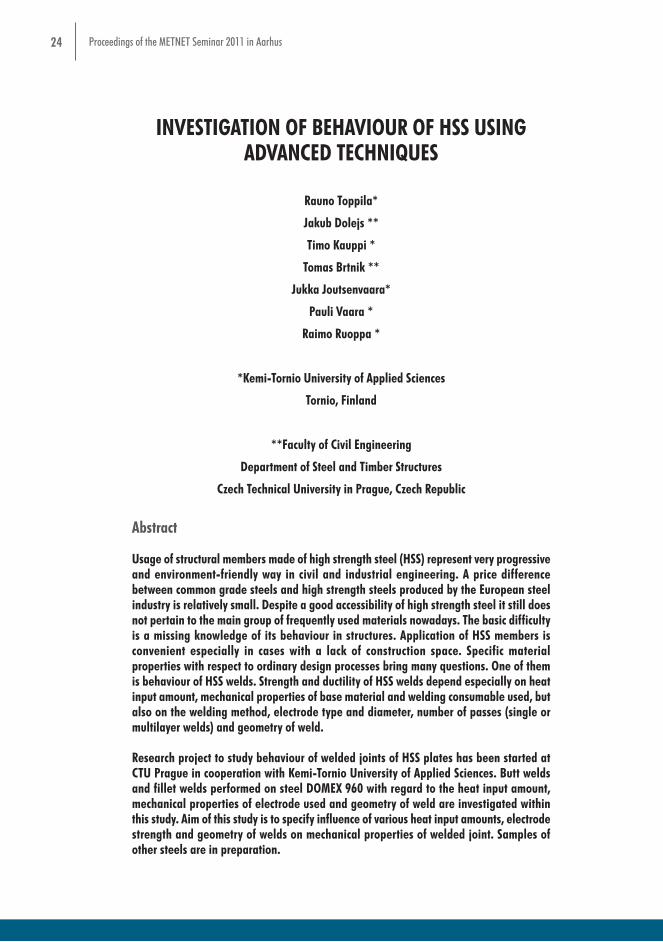
Usage of structural members made of high strength steel (HSS) represent very progressive and environment-friendly way in civil and industrial engineering. A price difference between common grade steels and high strength steels produced by the European steel industry is relatively small. Despite a good accessibility of high strength steel it still does not pertain to the main group of frequently used materials nowadays. The basic difficulty is a missing knowledge of its behaviour in structures. Application of HSS members is convenient especially in cases with a lack of construction space. Specific material properties with respect to ordinary design processes bring many questions. One of them is behaviour of HSS welds. Strength and ductility of HSS welds depend especially on heat input amount, mechanical properties of base material and welding consumable used, but also on the welding method, electrode type and diameter, number of passes (single or multilayer welds) and geometry of weld.
Research project to study behaviour of welded joints of HSS plates has been started at CTU Prague in cooperation with Kemi-Tornio University of Applied Sciences. Butt welds and fillet welds performed on steel DOMEX 960 with regard to the heat input amount, mechanical properties of electrode used and geometry of weld are investigated within this study. Aim of this study is to specify influence of various heat input amounts, electrode strength and geometry of welds on mechanical properties of welded joint. Samples of other steels are in preparation.

25Proceedings of the METNET Seminar 2011 in Aarhus
There are also presented available new techniques for High and Ultra High Strength Steels (HSS and UHSS) weldments testing in the paper including optical measurement in tensile tests, springback measurement, crack propagation and idea of using hydroforming machine as a bending press.. GOM Aramis / Argus system is adapted to measure true strain distribution in tensile testing. In studying flangeability springback is measured real time using machine vision system. Machine vision technique is also applied in detecting cracking occurring in outer edge of bended sample. At last an idea of adapting hydroforming machine to study flangeability of thick UHSS samples is presented.
High Strength Steel
New or improved techniqes of steel processing such as Thermo-Mechanically Controlled Processing (TMCP) and Quenching in conjunction with Tempering (QT) led to availability of High Strength Steels with low alloy content and good weldability in last few years. On the market there are steels matching much higher grades than is covered by design codes. New European design codes for Civil Engineering allow using steels up to grade S700. Nevertheless there are steel grades exceeding tensile strength 1300 MPa. According to lack of sufficient knowledge about behavior of HSS joints full utilization and material savings is hard to achieve. Current design rules covering HSS are also conservative in some cases [1,2].
Welds of High Strength Steel
With higher strength come hand in hand harder technological requirements on fabrication especially on welding. Design of HSS welded joint has to cover detailed scheduling of welding process concerning heat input. Strength of HSS welded joint is dependent besides heat input on electrode strength, dimensions of plate welded and end-shape of plate (amount of weld metal deposited) as well. The overall strength of the joint strongly depends on dimensions of Heat Affected Zone (HAZ) in case that higher heat input was used. Mechanical properties of the weld and heat affected zone is related to the microstructure, i.e. type, size distribution, morphology and volume fraction of various micro-structural constituents, whereas microstructure is strongly dependent on the chemical composition and processing conditions, especially on the cooling rate t
8/5. Heat input is basic factor influencing the cooling rate, which affects
mechanical properties and metallurgical structure of the weld and HAZ. Amount of heat input corresponds with the ratio of used power (current and voltage) to the welding speed. Heat input strongly influences the strength and toughness of the weld. The optimal heat input depends on the composition of the steel. Rules for suitable electrodes and levels of arc energy are provided by steel producers. Too low heat input results in cracks, on the other hand too high heat input decreases toughness and creates wider zone of undermatched strength in HAZ. A narrow zone of undermatching strength does not affect the strength of weld connection. According to requirements for heat input, range for cooling rates (t
8/5,MIN ; t
8/5,MAX ) can be calculated. After specifying a
minimal preheat temperature and maximal interpass temperature, working

26 Proceedings of the METNET Seminar 2011 in Aarhus
area of weld than can be plotted. These working areas are shown for steels S355 and HSS S960QL in Figures 1 and 2. For commonly used HSS, the t
8/5
can vary between 5 and 20 seconds, which corresponds with heat input in range from 0,6 up to 2,5 kJ/mm of weld [3,4,5].
Fig. 1 – Working area for S355 [3] Fig. 2 – Working area for S960 QL [3]
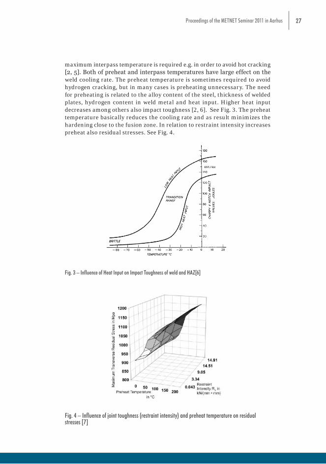
Tp corresponds to the minimum preheat temperature and expression interpass stands for Interpass temperature, which refers to the temperature of the steel just prior to the depositing of another weld pass. As a minimum interpass temperature is specified, welding should not be performed when the base plate is below this temperature. Steel must be heated back up before welding continues. A maximum interpass temperature may be specified to prevent deterioration of the weld metal and heat affected zone properties. In this case, steel must be below this temperature before welding continues. A specific maximum interpass temperature is required e.g. in order to avoid hot cracking [2, 5]. Both of preheat and interpass temperatures have large effect on the weld cooling rate. The preheat temperature is sometimes required to avoid hydrogen cracking, but in many cases is preheating unnecessary. The need for preheating is related to the alloy content of the steel, thickness of welded plates, hydrogen content in weld metal and heat input. Higher heat input decreases among others also impact toughness [2, 6]. See Fig. 3. The preheat temperature basically reduces the cooling rate and as result minimizes the hardening close to the fusion zone. In relation to restraint intensity increases preheat also residual stresses. See Fig. 4.
Fig. 3 – Influence of Heat Input on Impact Toughness of weld and HAZ[6]
Fig. 4 – Influence of joint toughness (restraint intensity) and preheat temperature on residual stresses [7]
Mechanical properties of weld parts can remarkable change within the work area of weld even if all requirements for welding were fulfilled. With increase of t8/5, strength, toughness and hardness decreases and ductility increases. The higher the steel grade the larger the difference between boundary values if the same cooling rates are used [3, 4, 5]. See Fig. 5 and 6.
Fig. 1 – Working area for S355 [3]
Fig. 1 – Working area for S355 [3] Fig. 2 – Working area for S960 QL [3]
Tp corresponds to the minimum preheat temperature and expression interpass stands for Interpass temperature, which refers to the temperature of the steel just prior to the depositing of another weld pass. As a minimum interpass temperature is specified, welding should not be performed when the base plate is below this temperature. Steel must be heated back up before welding continues. A maximum interpass temperature may be specified to prevent deterioration of the weld metal and heat affected zone properties. In this case, steel must be below this temperature before welding continues. A specific maximum interpass temperature is required e.g. in order to avoid hot cracking [2, 5]. Both of preheat and interpass temperatures have large effect on the weld cooling rate. The preheat temperature is sometimes required to avoid hydrogen cracking, but in many cases is preheating unnecessary. The need for preheating is related to the alloy content of the steel, thickness of welded plates, hydrogen content in weld metal and heat input. Higher heat input decreases among others also impact toughness [2, 6]. See Fig. 3. The preheat temperature basically reduces the cooling rate and as result minimizes the hardening close to the fusion zone. In relation to restraint intensity increases preheat also residual stresses. See Fig. 4.
Fig. 3 – Influence of Heat Input on Impact Toughness of weld and HAZ[6]
Fig. 4 – Influence of joint toughness (restraint intensity) and preheat temperature on residual stresses [7]
Mechanical properties of weld parts can remarkable change within the work area of weld even if all requirements for welding were fulfilled. With increase of t8/5, strength, toughness and hardness decreases and ductility increases. The higher the steel grade the larger the difference between boundary values if the same cooling rates are used [3, 4, 5]. See Fig. 5 and 6.
Fig. 2 – Working area for S960 QL [3]
Tp corresponds to the minimum preheat temperature and expression interpass
stands for Interpass temperature, which refers to the temperature of the steel just prior to the depositing of another weld pass. As a minimum interpass temperature is specified, welding should not be performed when the base plate is below this temperature. Steel must be heated back up before welding continues. A maximum interpass temperature may be specified to prevent deterioration of the weld metal and heat affected zone properties. In this case, steel must be below this temperature before welding continues. A specific
27Proceedings of the METNET Seminar 2011 in Aarhus
maximum interpass temperature is required e.g. in order to avoid hot cracking [2, 5]. Both of preheat and interpass temperatures have large effect on the weld cooling rate. The preheat temperature is sometimes required to avoid hydrogen cracking, but in many cases is preheating unnecessary. The need for preheating is related to the alloy content of the steel, thickness of welded plates, hydrogen content in weld metal and heat input. Higher heat input decreases among others also impact toughness [2, 6]. See Fig. 3. The preheat temperature basically reduces the cooling rate and as result minimizes the hardening close to the fusion zone. In relation to restraint intensity increases preheat also residual stresses. See Fig. 4.
Fig. 1 – Working area for S355 [3] Fig. 2 – Working area for S960 QL [3]
Tp corresponds to the minimum preheat temperature and expression interpass stands for Interpass temperature, which refers to the temperature of the steel just prior to the depositing of another weld pass. As a minimum interpass temperature is specified, welding should not be performed when the base plate is below this temperature. Steel must be heated back up before welding continues. A maximum interpass temperature may be specified to prevent deterioration of the weld metal and heat affected zone properties. In this case, steel must be below this temperature before welding continues. A specific maximum interpass temperature is required e.g. in order to avoid hot cracking [2, 5]. Both of preheat and interpass temperatures have large effect on the weld cooling rate. The preheat temperature is sometimes required to avoid hydrogen cracking, but in many cases is preheating unnecessary. The need for preheating is related to the alloy content of the steel, thickness of welded plates, hydrogen content in weld metal and heat input. Higher heat input decreases among others also impact toughness [2, 6]. See Fig. 3. The preheat temperature basically reduces the cooling rate and as result minimizes the hardening close to the fusion zone. In relation to restraint intensity increases preheat also residual stresses. See Fig. 4.
Fig. 3 – Influence of Heat Input on Impact Toughness of weld and HAZ[6]
Fig. 4 – Influence of joint toughness (restraint intensity) and preheat temperature on residual stresses [7]
Mechanical properties of weld parts can remarkable change within the work area of weld even if all requirements for welding were fulfilled. With increase of t8/5, strength, toughness and hardness decreases and ductility increases. The higher the steel grade the larger the difference between boundary values if the same cooling rates are used [3, 4, 5]. See Fig. 5 and 6.
Fig. 3 – Influence of Heat Input on Impact Toughness of weld and HAZ[6]
Fig. 1 – Working area for S355 [3] Fig. 2 – Working area for S960 QL [3]
Tp corresponds to the minimum preheat temperature and expression interpass stands for Interpass temperature, which refers to the temperature of the steel just prior to the depositing of another weld pass. As a minimum interpass temperature is specified, welding should not be performed when the base plate is below this temperature. Steel must be heated back up before welding continues. A maximum interpass temperature may be specified to prevent deterioration of the weld metal and heat affected zone properties. In this case, steel must be below this temperature before welding continues. A specific maximum interpass temperature is required e.g. in order to avoid hot cracking [2, 5]. Both of preheat and interpass temperatures have large effect on the weld cooling rate. The preheat temperature is sometimes required to avoid hydrogen cracking, but in many cases is preheating unnecessary. The need for preheating is related to the alloy content of the steel, thickness of welded plates, hydrogen content in weld metal and heat input. Higher heat input decreases among others also impact toughness [2, 6]. See Fig. 3. The preheat temperature basically reduces the cooling rate and as result minimizes the hardening close to the fusion zone. In relation to restraint intensity increases preheat also residual stresses. See Fig. 4.
Fig. 3 – Influence of Heat Input on Impact Toughness of weld and HAZ[6]
Fig. 4 – Influence of joint toughness (restraint intensity) and preheat temperature on residual stresses [7]
Mechanical properties of weld parts can remarkable change within the work area of weld even if all requirements for welding were fulfilled. With increase of t8/5, strength, toughness and hardness decreases and ductility increases. The higher the steel grade the larger the difference between boundary values if the same cooling rates are used [3, 4, 5]. See Fig. 5 and 6.
Fig. 4 – Influence of joint toughness (restraint intensity) and preheat temperature on residual stresses [7]
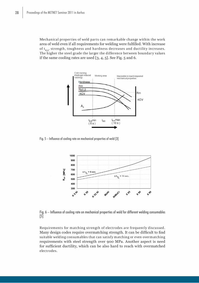
28 Proceedings of the METNET Seminar 2011 in Aarhus
Mechanical properties of weld parts can remarkable change within the work area of weld even if all requirements for welding were fulfilled. With increase of t
8/5, strength, toughness and hardness decreases and ductility increases.
The higher the steel grade the larger the difference between boundary values if the same cooling rates are used [3, 4, 5]. See Fig. 5 and 6.
Fig. 5 – Influence of cooling rate on mechanical properties of weld [3]
Fig. 6 – Influence of cooling rate on mechanical properties of weld for different welding consumables [5]
Requirements for matching strength of electrodes are frequently discussed. Many design codes require overmatching strength. It can be difficult to find suitable welding consumables that can satisfy matching or even overmatching requirements with steel strength over 900 MPa. Another aspect is need for sufficient ductility, which can be also hard to reach with overmatched electrodes.
The possibility, how to simplify welding of HSS is to use undermatched electrodes. Using electrodes with lower strength than parent material makes welds more ductile and less prone to cracking. One of the advantages of undermatched weld metal is also a lower heat input and therefore lowers residual stresses. Next to this, undermatched weld metal also allows to decrease preheat temperature and thereby fabrication costs. Matching weld metal may reduce overall weld quality, increasing distortion, residual stresses and cracking tendencies, including lamellar tearing. It was shown in various tensile tests of undermatched welds that the undermatched weld metal does not behave in the same way as the unrestricted metal. Its properties are elevated due to the restraint effect provided by the base metal and the tri-axial state of stress in welded joint. Undermatched electrodes are allowed in EN 1993-1-12. [10]
Current research of HSS Welds at CTU
Research of welded HSS Domex 960 has been started at Czech Technical University in cooperation with Kemi-Tornio University of Applied Sciences (Fig 7, 8). One steel grade, butt welds as well as fillet welds, three electrodes and three heat inputs are tested. One matching and two undermatched electrodes are used for welding of samples. New testing methods described in chapter 4 will be used for research that will follow first tests.
Fig. 5 – Influence of cooling rate on mechanical properties of weld [3]
Fig. 5 – Influence of cooling rate on mechanical properties of weld [3]
Fig. 6 – Influence of cooling rate on mechanical properties of weld for different welding consumables [5]
Requirements for matching strength of electrodes are frequently discussed. Many design codes require overmatching strength. It can be difficult to find suitable welding consumables that can satisfy matching or even overmatching requirements with steel strength over 900 MPa. Another aspect is need for sufficient ductility, which can be also hard to reach with overmatched electrodes.
The possibility, how to simplify welding of HSS is to use undermatched electrodes. Using electrodes with lower strength than parent material makes welds more ductile and less prone to cracking. One of the advantages of undermatched weld metal is also a lower heat input and therefore lowers residual stresses. Next to this, undermatched weld metal also allows to decrease preheat temperature and thereby fabrication costs. Matching weld metal may reduce overall weld quality, increasing distortion, residual stresses and cracking tendencies, including lamellar tearing. It was shown in various tensile tests of undermatched welds that the undermatched weld metal does not behave in the same way as the unrestricted metal. Its properties are elevated due to the restraint effect provided by the base metal and the tri-axial state of stress in welded joint. Undermatched electrodes are allowed in EN 1993-1-12. [10]
Current research of HSS Welds at CTU
Research of welded HSS Domex 960 has been started at Czech Technical University in cooperation with Kemi-Tornio University of Applied Sciences (Fig 7, 8). One steel grade, butt welds as well as fillet welds, three electrodes and three heat inputs are tested. One matching and two undermatched electrodes are used for welding of samples. New testing methods described in chapter 4 will be used for research that will follow first tests.
Fig. 6 – Influence of cooling rate on mechanical properties of weld for different welding consumables [5]
Requirements for matching strength of electrodes are frequently discussed. Many design codes require overmatching strength. It can be difficult to find suitable welding consumables that can satisfy matching or even overmatching requirements with steel strength over 900 MPa. Another aspect is need for sufficient ductility, which can be also hard to reach with overmatched electrodes.
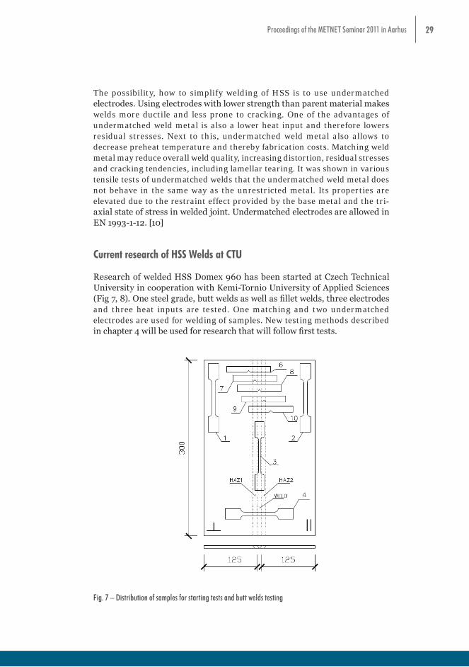
29Proceedings of the METNET Seminar 2011 in Aarhus
The possibility, how to simplify welding of HSS is to use undermatched electrodes. Using electrodes with lower strength than parent material makes welds more ductile and less prone to cracking. One of the advantages of undermatched weld metal is also a lower heat input and therefore lowers residual stresses. Next to this, undermatched weld metal also allows to decrease preheat temperature and thereby fabrication costs. Matching weld metal may reduce overall weld quality, increasing distortion, residual stresses and cracking tendencies, including lamellar tearing. It was shown in various tensile tests of undermatched welds that the undermatched weld metal does not behave in the same way as the unrestricted metal. Its properties are elevated due to the restraint effect provided by the base metal and the tri-axial state of stress in welded joint. Undermatched electrodes are allowed in EN 1993-1-12. [10]
Current research of HSS Welds at CTU
Research of welded HSS Domex 960 has been started at Czech Technical University in cooperation with Kemi-Tornio University of Applied Sciences (Fig 7, 8). One steel grade, butt welds as well as fillet welds, three electrodes and three heat inputs are tested. One matching and two undermatched electrodes are used for welding of samples. New testing methods described in chapter 4 will be used for research that will follow first tests.
Fig. 7 – Distribution of samples for starting tests and butt welds testing
Fig. 8 – Samples for fillet welds testing
New Techniques to study HSS
In this article is presented some studies of HSS welds and methods to test High Strength Steels. First GOM Aramis / Argus system to measure stress and strain in tensile test in base material and in weld and HAZ area. Next measuring method is springback measurement using machine vision system. Machine vision is also used in next application which is crack detection. Last one is an idea how hydroforming machine is used as bending press to study thick materials flangeability.
GOM Aramis / Argus
One quite prominent of those is full field strain analysis with optical measurement system. With non-contacting measurement it is possible to measure areas up from roughly 200 square millimeters. Area depends of used equipment combination and measuring distances. Each camera has 5mpix resolution that can be used to capture images from different stages of tests. With smaller capture areas it is possible to capture deformations in smaller area with very high resolution and accuracy. With testing of welded specimens it is possible to isolate certain areas in a weld, namely HAZ and weld itself, by measuring the strains during the test. Also with continuous image capturing it is possible to gain insight about the appearing and change of different stages of necking, i.e. from diffuse necking to localized necking before eventual breakage of specimen. The global strain over weld can be verified with this kind of measuring system and it also provides comparison method for extensometer data from tensile test machine. Weld seam orientation within specimen series can be used to get results of different load bearing capabilities in different directions, most commonly in 0, 30, 45, 60, 90 degrees in relation to specimen length. Figure 9 shows the development of strain concentration below the weld during normal tensile test.
Fig. 7 – Distribution of samples for starting tests and butt welds testing
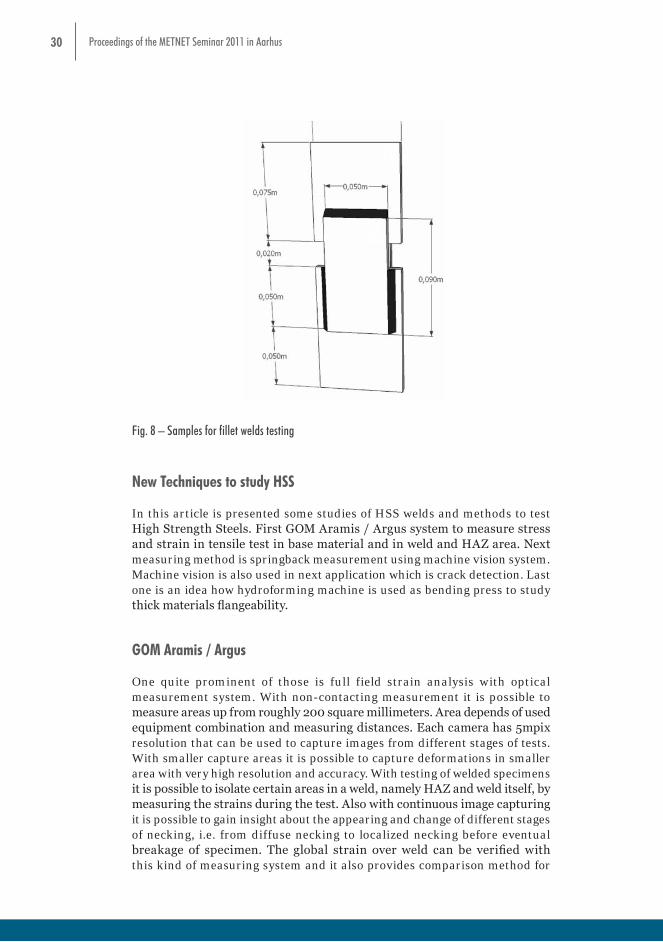
30 Proceedings of the METNET Seminar 2011 in Aarhus
Fig. 7 – Distribution of samples for starting tests and butt welds testing
Fig. 8 – Samples for fillet welds testing
New Techniques to study HSS
In this article is presented some studies of HSS welds and methods to test High Strength Steels. First GOM Aramis / Argus system to measure stress and strain in tensile test in base material and in weld and HAZ area. Next measuring method is springback measurement using machine vision system. Machine vision is also used in next application which is crack detection. Last one is an idea how hydroforming machine is used as bending press to study thick materials flangeability.
GOM Aramis / Argus
One quite prominent of those is full field strain analysis with optical measurement system. With non-contacting measurement it is possible to measure areas up from roughly 200 square millimeters. Area depends of used equipment combination and measuring distances. Each camera has 5mpix resolution that can be used to capture images from different stages of tests. With smaller capture areas it is possible to capture deformations in smaller area with very high resolution and accuracy. With testing of welded specimens it is possible to isolate certain areas in a weld, namely HAZ and weld itself, by measuring the strains during the test. Also with continuous image capturing it is possible to gain insight about the appearing and change of different stages of necking, i.e. from diffuse necking to localized necking before eventual breakage of specimen. The global strain over weld can be verified with this kind of measuring system and it also provides comparison method for extensometer data from tensile test machine. Weld seam orientation within specimen series can be used to get results of different load bearing capabilities in different directions, most commonly in 0, 30, 45, 60, 90 degrees in relation to specimen length. Figure 9 shows the development of strain concentration below the weld during normal tensile test.
Fig. 8 – Samples for fillet welds testing
New Techniques to study HSS
In this article is presented some studies of HSS welds and methods to test High Strength Steels. First GOM Aramis / Argus system to measure stress and strain in tensile test in base material and in weld and HAZ area. Next measuring method is springback measurement using machine vision system. Machine vision is also used in next application which is crack detection. Last one is an idea how hydroforming machine is used as bending press to study thick materials flangeability.
GOM Aramis / Argus
One quite prominent of those is full field strain analysis with optical measurement system. With non-contacting measurement it is possible to measure areas up from roughly 200 square millimeters. Area depends of used equipment combination and measuring distances. Each camera has 5mpix resolution that can be used to capture images from different stages of tests. With smaller capture areas it is possible to capture deformations in smaller area with very high resolution and accuracy. With testing of welded specimens it is possible to isolate certain areas in a weld, namely HAZ and weld itself, by measuring the strains during the test. Also with continuous image capturing it is possible to gain insight about the appearing and change of different stages of necking, i.e. from diffuse necking to localized necking before eventual breakage of specimen. The global strain over weld can be verified with this kind of measuring system and it also provides comparison method for

31Proceedings of the METNET Seminar 2011 in Aarhus
extensometer data from tensile test machine. Weld seam orientation within specimen series can be used to get results of different load bearing capabilities in different directions, most commonly in 0, 30, 45, 60, 90 degrees in relation to specimen length. Figure 9 shows the development of strain concentration below the weld during normal tensile test.
Fig. 9 - Strain stages during tensile test of welded specimen
Springback measurement using machine vision
In bending process, there is a need to measure exactly the produced angle. This is due to the fact that after the forming pressure is released, springback effect will occur. The magnitude of the springback effect depends mainly on material strength, thickness and strain hardening. To get the sheet to remain in the desired angle after the bending process, one must know how much deeper angle has to be produced temporarily during the process to compensate for the springback. To be able to adjust for the variation between different steel qualities, a machine vision method has been developed to measure the angle reached in bending while the forming pressure by the pressing tool is still on, and again after the pressure has been released. The measurement system comprises of camera and foreground light installed in one end of the pressing tool. The edge of the sheet visible to the camera has to be painted white before bending in order to make the edge more reflective. The more the edge reflects light the better contrast is gained between the sheet and the bending tool. Ideally the sheet edge would appear white in the resulting image, while the surroundings would appear black. From the image, angle between the two straight halves of the edge on both sides of the bent spot is measured.
Fig. 10 - Pressing tool and measurement equipment. On the left there is the steel sheet
being bent. On the right there are the light assembly and camera.
Fig. 11 - Angle measurement process. Software detects straight parts of the sheet and computes angle between them.
Fig. 9 - Strain stages during tensile test of welded specimen
Springback measurement using machine vision
In bending process, there is a need to measure exactly the produced angle. This is due to the fact that after the forming pressure is released, springback effect will occur. The magnitude of the springback effect depends mainly on material strength, thickness and strain hardening. To get the sheet to remain in the desired angle after the bending process, one must know how much deeper angle has to be produced temporarily during the process to compensate for the springback. To be able to adjust for the variation between different steel qualities, a machine vision method has been developed to measure the angle reached in bending while the forming pressure by the pressing tool is still on, and again after the pressure has been released. The measurement system comprises of camera and foreground light installed in one end of the pressing tool. The edge of the sheet visible to the camera has to be painted white before bending in order to make the edge more reflective. The more the edge reflects light the better contrast is gained between the sheet and the bending tool. Ideally the sheet edge would appear white in the resulting image, while the surroundings would appear black. From the image, angle between the two straight halves of the edge on both sides of the bent spot is measured.

32 Proceedings of the METNET Seminar 2011 in Aarhus
Fig. 9 - Strain stages during tensile test of welded specimen
Springback measurement using machine vision
In bending process, there is a need to measure exactly the produced angle. This is due to the fact that after the forming pressure is released, springback effect will occur. The magnitude of the springback effect depends mainly on material strength, thickness and strain hardening. To get the sheet to remain in the desired angle after the bending process, one must know how much deeper angle has to be produced temporarily during the process to compensate for the springback. To be able to adjust for the variation between different steel qualities, a machine vision method has been developed to measure the angle reached in bending while the forming pressure by the pressing tool is still on, and again after the pressure has been released. The measurement system comprises of camera and foreground light installed in one end of the pressing tool. The edge of the sheet visible to the camera has to be painted white before bending in order to make the edge more reflective. The more the edge reflects light the better contrast is gained between the sheet and the bending tool. Ideally the sheet edge would appear white in the resulting image, while the surroundings would appear black. From the image, angle between the two straight halves of the edge on both sides of the bent spot is measured.
Fig. 10 - Pressing tool and measurement equipment. On the left there is the steel sheet
being bent. On the right there are the light assembly and camera.
Fig. 11 - Angle measurement process. Software detects straight parts of the sheet and computes angle between them. Fig. 10 - Pressing tool and measurement equipment. On the left there is the steel sheet being bent. On the
right there are the light assembly and camera.
Fig. 9 - Strain stages during tensile test of welded specimen
Springback measurement using machine vision
In bending process, there is a need to measure exactly the produced angle. This is due to the fact that after the forming pressure is released, springback effect will occur. The magnitude of the springback effect depends mainly on material strength, thickness and strain hardening. To get the sheet to remain in the desired angle after the bending process, one must know how much deeper angle has to be produced temporarily during the process to compensate for the springback. To be able to adjust for the variation between different steel qualities, a machine vision method has been developed to measure the angle reached in bending while the forming pressure by the pressing tool is still on, and again after the pressure has been released. The measurement system comprises of camera and foreground light installed in one end of the pressing tool. The edge of the sheet visible to the camera has to be painted white before bending in order to make the edge more reflective. The more the edge reflects light the better contrast is gained between the sheet and the bending tool. Ideally the sheet edge would appear white in the resulting image, while the surroundings would appear black. From the image, angle between the two straight halves of the edge on both sides of the bent spot is measured.
Fig. 10 - Pressing tool and measurement equipment. On the left there is the steel sheet
being bent. On the right there are the light assembly and camera.
Fig. 11 - Angle measurement process. Software detects straight parts of the sheet and computes angle between them. Fig. 11 - Angle measurement process. Software detects straight parts of the sheet and computes
angle between them.
Crack detection using machine vision
Machine vision was tested also in detecting cracks from bending process, and a promising method was found. In the method, on the outside of the bend, light was cast diagonally from two opposite directions, and image was taken with a camera pointing directly at the bend. The image was taken in such direction that the bend and possible cracks appeared vertically. On the image, averages of grayscale values of each column of pixels were computed. The set of the averages was taken into a graph for which a 9th-degree polynomial was fitted. Average of the variance between values of the original graph and values of the polynomial was computed. A correlation was found between this value and manual findings on the bent slab samples: the averages were higher in cases of more seriously cracked samples than in cases of less cracked samples.
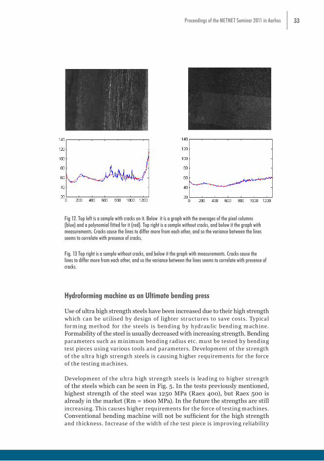
33Proceedings of the METNET Seminar 2011 in Aarhus
Crack detection using machine vision
Machine vision was tested also in detecting cracks from bending process, and a promising method was found. In the method, on the outside of the bend, light was cast diagonally from two opposite directions, and image was taken with a camera pointing directly at the bend. The image was taken in such direction that the bend and possible cracks appeared vertically. On the image, averages of grayscale values of each column of pixels were computed. The set of the averages was taken into a graph for which a 9th-degree polynomial was fitted. Average of the variance between values of the original graph and values of the polynomial was computed. A correlation was found between this value and manual findings on the bent slab samples: the averages were higher in cases of more seriously cracked samples than in cases of less cracked samples.
Fig 12. Top left is a sample with cracks on it. Below it is a graph with the averages of the pixel columns (blue) and a polynomial fitted for it (red). Top right is a sample without cracks, and below it the graph with measurements. Cracks cause the lines to differ more from each other, and so the variance between the lines seems to correlate with presence of cracks.
Fig. 13 Top right is a sample without cracks, and below it the graph with measurements. Cracks cause the lines to differ more from each other, and so the variance between the lines seems to correlate with presence of cracks.
Hydroforming machine as an Ultimate bending press
Use of ultra high strength steels have been increased due to their high strength which can be utilised by design of lighter structures to save costs. Typical forming method for the steels is bending by hydraulic bending machine. Formability of the steel is usually decreased with increasing strength. Bending parameters such as minimum bending radius etc. must be tested by bending test pieces using various tools and parameters. Development of the strength of the ultra high strength steels is causing higher requirements for the force of the testing machines.
Development of the ultra high strength steels is leading to higher strength of the steels which can be seen in Fig. 5. In the tests previously mentioned, highest strength of the steel was 1250 MPa (Raex 400), but Raex 500 is already in the market (Rm = 1600 MPa). In the future the strengths are still increasing. This causes higher requirements for the force of testing machines. Conventional bending machine will not be sufficient for the high strength and thickness. Increase of the width of the test piece is improving reliability
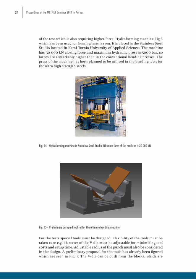
34 Proceedings of the METNET Seminar 2011 in Aarhus
of the test which is also requiring higher force. Hydroforming machine Fig 6 which has been used for forming tests is seen. It is placed in the Stainless Steel Studio located in Kemi-Tornio University of Applied Sciences The machine has 30 000 kN closing force and maximum hydraulic press is 5000 bar, so forces are remarkably higher than in the conventional bending presses. The press of the machine has been planned to be utilised in the bending tests for the ultra high strength steels.
Development of the ultra high strength steels is leading to higher strength of the steels which can be seen in Fig. 5. In the tests previously mentioned, highest strength of the steel was 1250 MPa (Raex 400), but Raex 500 is already in the market (Rm = 1600 MPa). In the future the strengths are still increasing. This causes higher requirements for the force of testing machines. Conventional bending machine will not be sufficient for the high strength and thickness. Increase of the width of the test piece is improving reliability of the test which is also requiring higher force. Hydroforming machine Fig 6 which has been used for forming tests is seen. It is placed in the Stainless Steel Studio located in Kemi-Tornio University of Applied Sciences The machine has 30 000 kN closing force and maximum hydraulic press is 5000 bar, so forces are remarkably higher than in the conventional bending presses. The press of the machine has been planned to be utilised in the bending tests for the ultra high strength steels.
Fig. 14 - Hydroforming machine in Stainless Steel Studio. Ultimate force of the machine is
30 000 kN.
Fig. 15 - Preliminary designed tool set for the ultimate bending machine.
For the tests special tools must be designed. Flexibility of the tools must be taken care e.g. diameter of the V-die must be adjustable for minimizing tool costs and setup time. Adjustable radius of the punch must also be considered in the design. A preliminary proposal for the tools has already been figured which are seen in Fig. 7. The V-die can be built from the blocks, which are moving transversely to the bending line allowing the diameter of the V-die being adjustable. In this tool set, the radius of the punch is able to be up to 100…300 mm and the diameter of the V-die 300…700 mm. This enables remarkably higher strength and thickness as well as width of the materials been tested compared to the current testing methods, which is necessary in the future bending tests.
Fig. 14 - Hydroforming machine in Stainless Steel Studio. Ultimate force of the machine is 30 000 kN.
Development of the ultra high strength steels is leading to higher strength of the steels which can be seen in Fig. 5. In the tests previously mentioned, highest strength of the steel was 1250 MPa (Raex 400), but Raex 500 is already in the market (Rm = 1600 MPa). In the future the strengths are still increasing. This causes higher requirements for the force of testing machines. Conventional bending machine will not be sufficient for the high strength and thickness. Increase of the width of the test piece is improving reliability of the test which is also requiring higher force. Hydroforming machine Fig 6 which has been used for forming tests is seen. It is placed in the Stainless Steel Studio located in Kemi-Tornio University of Applied Sciences The machine has 30 000 kN closing force and maximum hydraulic press is 5000 bar, so forces are remarkably higher than in the conventional bending presses. The press of the machine has been planned to be utilised in the bending tests for the ultra high strength steels.
Fig. 14 - Hydroforming machine in Stainless Steel Studio. Ultimate force of the machine is
30 000 kN.
Fig. 15 - Preliminary designed tool set for the ultimate bending machine.
For the tests special tools must be designed. Flexibility of the tools must be taken care e.g. diameter of the V-die must be adjustable for minimizing tool costs and setup time. Adjustable radius of the punch must also be considered in the design. A preliminary proposal for the tools has already been figured which are seen in Fig. 7. The V-die can be built from the blocks, which are moving transversely to the bending line allowing the diameter of the V-die being adjustable. In this tool set, the radius of the punch is able to be up to 100…300 mm and the diameter of the V-die 300…700 mm. This enables remarkably higher strength and thickness as well as width of the materials been tested compared to the current testing methods, which is necessary in the future bending tests.
Fig. 15 - Preliminary designed tool set for the ultimate bending machine.
For the tests special tools must be designed. Flexibility of the tools must be taken care e.g. diameter of the V-die must be adjustable for minimizing tool costs and setup time. Adjustable radius of the punch must also be considered in the design. A preliminary proposal for the tools has already been figured which are seen in Fig. 7. The V-die can be built from the blocks, which are
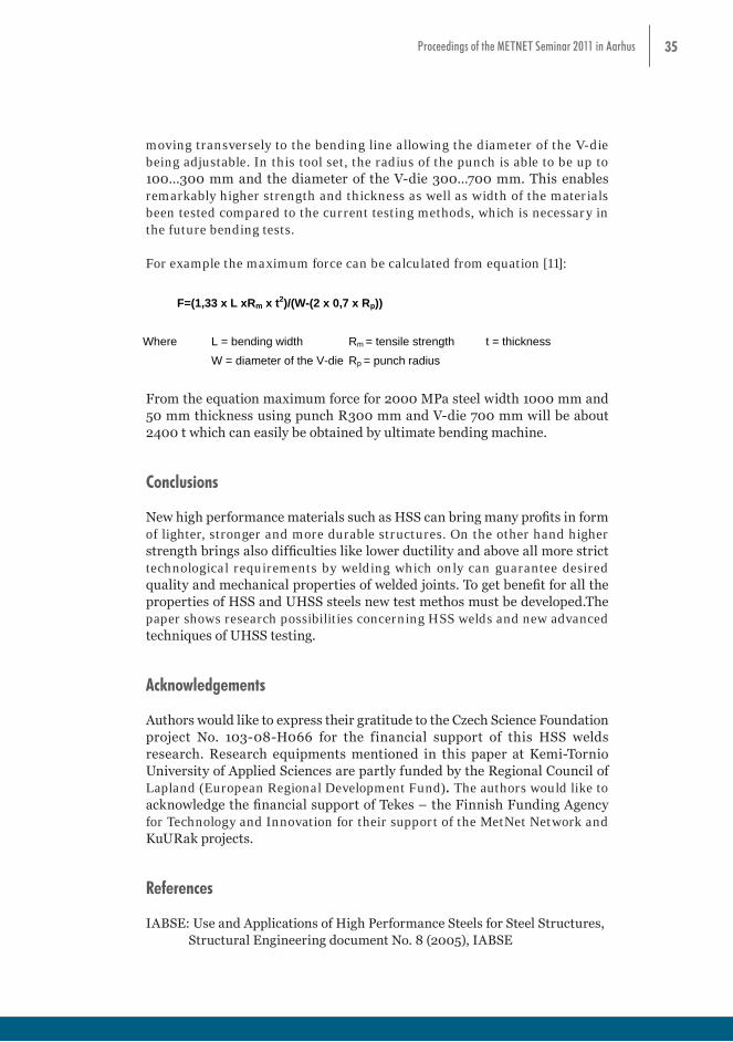
35Proceedings of the METNET Seminar 2011 in Aarhus
moving transversely to the bending line allowing the diameter of the V-die being adjustable. In this tool set, the radius of the punch is able to be up to 100…300 mm and the diameter of the V-die 300…700 mm. This enables remarkably higher strength and thickness as well as width of the materials been tested compared to the current testing methods, which is necessary in the future bending tests.
For example the maximum force can be calculated from equation [11]:For example the maximum force can be calculated from equation [11]: F=(1,33 x L xRm x t2)/(W-(2 x 0,7 x Rp)) Where L = bending width Rm = tensile strength t = thickness W = diameter of the V-die Rp = punch radius From the equation maximum force for 2000 MPa steel width 1000 mm and 50 mm thickness using punch R300 mm and V-die 700 mm will be about 2400 t which can easily be obtained by ultimate bending machine. Conclusions New high performance materials such as HSS can bring many profits in form of lighter, stronger and more durable structures. On the other hand higher strength brings also difficulties like lower ductility and above all more strict technological requirements by welding which only can guarantee desired quality and mechanical properties of welded joints. To get benefit for all the properties of HSS and UHSS steels new test methos must be developed.The paper shows research possibilities concerning HSS welds and new advanced techniques of UHSS testing. Acknowledgements Authors would like to express their gratitude to the Czech Science Foundation project No. 103-08-H066 for the financial support of this HSS welds research. Research equipments mentioned in this paper at Kemi-Tornio University of Applied Sciences are partly funded by the Regional Council of Lapland (European Regional Development Fund). The authors would like to acknowledge the financial support of Tekes – the Finnish Funding Agency for Technology and Innovation for their support of the MetNet Network and KuURak projects. References IABSE: Use and Applications of High Performance Steels for Steel Structures, Structural Engineering document No. 8 (2005), IABSE Rasche C., Kuhlmann U.: Investigations on longitudinal fillet welded lap joints of HSS – NSCC 2009 Herman, P.: Welding of Fine-grained High-strength Steels, http://www.konstrukce.cz/clanek/svarovani-jemnozrnnych-vysokopevnostnich-oceli/ (2010) Gresnigt A. M., Steenhuis C. M.: High Strength Steels – Construction Research Communications Limited 1997, p. 31-41 Heuser H., Jochum C., Stracke E.: Weld metal as strong as base metal? , Mat.-wiss. u. Werkstofftech. 2007, 38, No.7
From the equation maximum force for 2000 MPa steel width 1000 mm and 50 mm thickness using punch R300 mm and V-die 700 mm will be about 2400 t which can easily be obtained by ultimate bending machine.
Conclusions
New high performance materials such as HSS can bring many profits in form of lighter, stronger and more durable structures. On the other hand higher strength brings also difficulties like lower ductility and above all more strict technological requirements by welding which only can guarantee desired quality and mechanical properties of welded joints. To get benefit for all the properties of HSS and UHSS steels new test methos must be developed.The paper shows research possibilities concerning HSS welds and new advanced techniques of UHSS testing.
Acknowledgements
Authors would like to express their gratitude to the Czech Science Foundation project No. 103-08-H066 for the financial support of this HSS welds research. Research equipments mentioned in this paper at Kemi-Tornio University of Applied Sciences are partly funded by the Regional Council of Lapland (European Regional Development Fund). The authors would like to acknowledge the financial support of Tekes – the Finnish Funding Agency for Technology and Innovation for their support of the MetNet Network and KuURak projects.
References
IABSE: Use and Applications of High Performance Steels for Steel Structures, Structural Engineering document No. 8 (2005), IABSE

36 Proceedings of the METNET Seminar 2011 in Aarhus
Rasche C., Kuhlmann U.: Investigations on longitudinal fillet welded lap joints of HSS – NSCC 2009
Herman, P.: Welding of Fine-grained High-strength Steels, http://www.konstrukce.cz/clanek/svarovani-jemnozrnnych-vysokopevnostnich-oceli/ (2010)
Gresnigt A. M., Steenhuis C. M.: High Strength Steels – Construction Research Communications Limited 1997, p. 31-41
Heuser H., Jochum C., Stracke E.: Weld metal as strong as base metal? , Mat.-wiss. u. Werkstofftech. 2007, 38, No.7
A. C. Davies : The Science and practice of welding, Vol. 1, Welding Science and technology, Cambridge University Press 2003, 363 p.
Kannengiesser T., Lausch T., Kromm A.: Effects of Heat Control on the Stress Build Up during High-Strength Steel Welding under Defined Restraint Conditions, Conference on HSS for Hydropower Plants / Takasaki, 2008
Collin, P. & Johansson, B.: Eurocode for HSS and Applications in Construction, 2005 Super-High Strength Steels: 1st international conference, 2 - 4 November 2005, Rome, Italy
EN 1993-1-8 Eurocode 3: Design of steel structures - Part 1-8: Design of joints, CEN, 2005
EN 1993-1-12 Eurocode 3 - Design of steel structures - Part 1-12: Additional rules for the extension of EN 1993 up to steel grades S 700, CEN, 2007
Trumpf manual: Technical information, Bending technology, 10/2006. TRUMPF Werkzeugmaschinen GmbH + Co. KG

37Proceedings of the METNET Seminar 2011 in Aarhus
CATENARY ACTION AND STRAINS OF WQ-BEAM IN OFFICE BUILDING DURING FIRE
Mikko Salminen
Karol Bzdawka
Tampere University of Technology
Abstract
In this study, the behaviour of a typical office building frame at elevated temperatures is studied numerically by using commercial finite element package ABAQUS. The frame consists of WQ-beams and composite columns. Exposed beam and column are modelled using shell and brick elements, respectively and geometrical and material non-linearities are taken into account. Protected and unprotected beams with hinged and semi-rigid joints to the column are considered. The non-uniform temperature distributions across the beam height are taken from fire tests. The results of non-linear analysis are compared to those obtained by using typical design procedure. The strains at the lower flange of the beam are reported for all cases.
Introduction
The idea of catenary action is not new, but it has only recently being considered in structural fire engineering [Yin, Wang, 2005]. The current design procedure of steel beams in fire is based on the bending resistance of the beam [EN 1993-1-2, 2005] and adopted from that at ambient temperature meaning that large deformations are not taken into account. This design philosophy leads to relatively low survival temperature and expensive fire protection is required [Yin, Wang, 2004]. The behaviour of a beam changes from bending to catenary action at large deflections and it can give the beam very high load carrying capacity compared to the design based on bending moment resistance. According to Wang [Yin, Wang, 2004], if large deflection is acceptable, it might be possible to eliminate fire protection to all steel beams in a building. However, it is important, that the effects of the catenary action to the adjacent structure and connections are taken into account.
Analysed frame
Numerical analyses were conducted for a non-sway frame shown in Figure 1 at ambient and fire temperatures. This kind of frame, where columns are
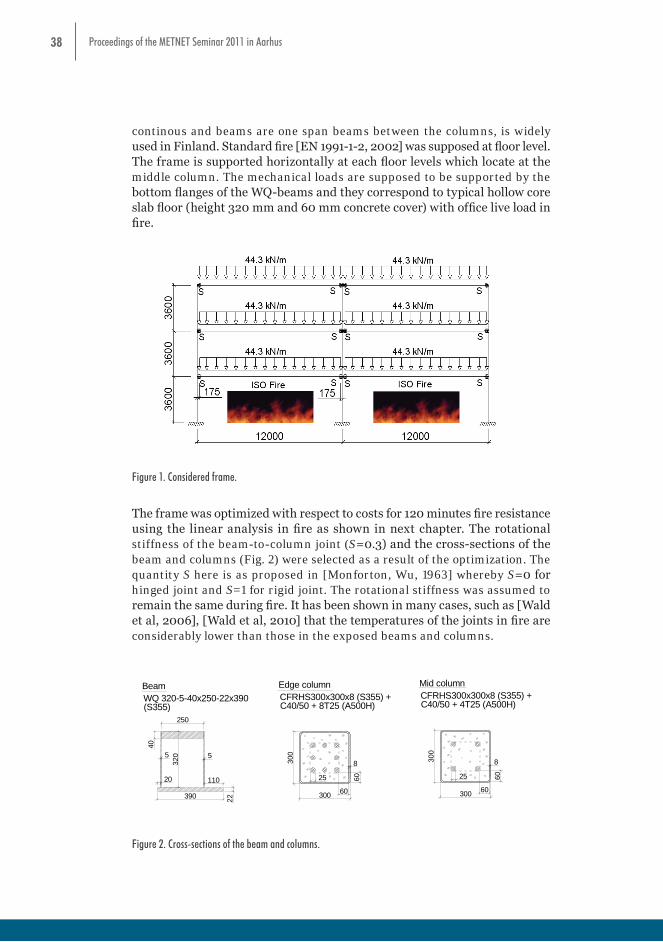
38 Proceedings of the METNET Seminar 2011 in Aarhus
continous and beams are one span beams between the columns, is widely used in Finland. Standard fire [EN 1991-1-2, 2002] was supposed at floor level. The frame is supported horizontally at each floor levels which locate at the middle column. The mechanical loads are supposed to be supported by the bottom flanges of the WQ-beams and they correspond to typical hollow core slab floor (height 320 mm and 60 mm concrete cover) with office live load in fire.
Figure 1. Considered frame.
The frame was optimized with respect to costs for 120 minutes fire resistance using the linear analysis in fire as shown in next chapter. The rotational stiffness of the beam-to-column joint (S=0.3) and the cross-sections of the beam and columns (Fig. 2) were selected as a result of the optimization. The quantity S here is as proposed in [Monforton, Wu, 1963] whereby S=0 for hinged joint and S=1 for rigid joint. The rotational stiffness was assumed to remain the same during fire. It has been shown in many cases, such as [Wald et al, 2006], [Wald et al, 2010] that the temperatures of the joints in fire are considerably lower than those in the exposed beams and columns.
60
6025
8300
300
Mid columnCFRHS300x300x8 (S355) +C40/50 + 4T25 (A500H)
BeamWQ 320-5-40x250-22x390(S355)
390 22
320 55
20 110
40
250
Edge columnCFRHS300x300x8 (S355) +C40/50 + 8T25 (A500H)
300
300
8
25 60
60
Figure 2. Cross-sections of the beam and columns.
Typical design procedure Standard design procedure follows the principles of EC 3, for beams, and EC 4, for columns. The hollow-core concrete slab was chosen from the manufacturer’s catalogue. Together with the required topping concrete it provided the load of 75.7 kN/m in normal and 44.3 kN/m in fire situation. The load is only on one side of the beam. The stiffening effect of the concrete floor was not taken in the account in this research. The semi rigid joint was not modelled but rather the ratio of joint’s rotational stiffness in comparison to beam bending stiffness was used in form proposed in [Monforton, Wu, 1963]. Static analysis of the frame was done using frame3D program [Jalkanen, 2007] written to Matlab [Matlab®, 2009].
Figure 1. Considered frame.
The frame was optimized with respect to costs for 120 minutes fire resistance using the linear analysis in fire as shown in next chapter. The rotational stiffness of the beam-to-column joint (S=0.3) and the cross-sections of the beam and columns (Fig. 2) were selected as a result of the optimization. The quantity S here is as proposed in [Monforton, Wu, 1963] whereby S=0 for hinged joint and S=1 for rigid joint. The rotational stiffness was assumed to remain the same during fire. It has been shown in many cases, such as [Wald et al, 2006], [Wald et al, 2010] that the temperatures of the joints in fire are considerably lower than those in the exposed beams and columns.
60
6025
8300
300
Mid columnCFRHS300x300x8 (S355) +C40/50 + 4T25 (A500H)
BeamWQ 320-5-40x250-22x390(S355)
390 22
320 55
20 110
40
250
Edge columnCFRHS300x300x8 (S355) +C40/50 + 8T25 (A500H)
300
300
8
25 60
60
Figure 2. Cross-sections of the beam and columns.
Typical design procedure Standard design procedure follows the principles of EC 3, for beams, and EC 4, for columns. The hollow-core concrete slab was chosen from the manufacturer’s catalogue. Together with the required topping concrete it provided the load of 75.7 kN/m in normal and 44.3 kN/m in fire situation. The load is only on one side of the beam. The stiffening effect of the concrete floor was not taken in the account in this research. The semi rigid joint was not modelled but rather the ratio of joint’s rotational stiffness in comparison to beam bending stiffness was used in form proposed in [Monforton, Wu, 1963]. Static analysis of the frame was done using frame3D program [Jalkanen, 2007] written to Matlab [Matlab®, 2009].
Figure 2. Cross-sections of the beam and columns.

39Proceedings of the METNET Seminar 2011 in Aarhus
Typical design procedure
Standard design procedure follows the principles of EC 3, for beams, and EC 4, for columns. The hollow-core concrete slab was chosen from the manufacturer’s catalogue. Together with the required topping concrete it provided the load of 75.7 kN/m in normal and 44.3 kN/m in fire situation. The load is only on one side of the beam. The stiffening effect of the concrete floor was not taken in the account in this research. The semi rigid joint was not modelled but rather the ratio of joint’s rotational stiffness in comparison to beam bending stiffness was used in form proposed in [Monforton, Wu, 1963]. Static analysis of the frame was done using frame3D program [Jalkanen, 2007] written to Matlab [Matlab®, 2009].
The design of WQ beam in ambient situation follows [TRY, 2009] which is based on EC 3 standards [EN 1993-1-1, 2005] and [EN 1993-1-2, 2005]. [TRY, 2009] highlights the necessity of checking the lower flange of the beam in lateral bending due to the fact that the load is applied to the outer part of the lower flange. Bending and shear resistance of the beam is validated in 21 points along the beam. There are 3 ways to calculate the beam’s bending resistance depending on the cross section class: class 1-2: plastic bending resistance; class 3: elastic bending resistance; and for a beam with flanges class 1 or 2 and webs class 3 plastic bending resistance is calculated with a part of the web omitted in the calculation (following clause 6.2.5 of [EN 1993-1-1, 2005]). Concrete filling the gap between the beam web and the hollow-core slab, together with the reinforcement anchoring the beam to the slab, prevents the beam’s rotation so the beam’s resistance to torsion did not need to be checked. As a simplification it has been assumed that the beam is sufficiently insulated in fire situation and thus the beam temperature does not exceed the critical temperature θ
a,cr that according to EN 1993-1-2 [EN 1993-
1-2, 2005] is a dependant of utilisation factor in fire situation µ0.
Column resistance is verified in both design situations at the bottom and top cross sections. Resistance check considers axial compression, bending and shear. Shear resistance is not usually verified in those kinds of columns but in this case it has to be since, due to the semi-rigid connections, high shear forces in columns develop. Column design in normal and fire situation follows [TRY, 2004]. The plastic axial resistance is calculated as the sum of resistances of all 3 elements (steel tube, concrete core and reinforcement). The maximal plastic bending resistance (M
max.Rd) is calculated with the respect to the symmetry
axis of the cross-section. It is the bending resistance of all 3 elements but only half of the cross-section of the concrete core is taken into account. Location of the neutral axis of the cross section is found from the force equilibrium in the cross-section. It is then used to calculate the plastic bending moment (M
pl.Rd). Proportion of M
max.Rd /M
pl.Rd is necessary for the calculation of µ using
graphical method. µ is used in the equation (1) for bending resistance of a cross section under compression [TRY, 2004]. α
M in eq. 1 is equal to 0.9.
40 Proceedings of the METNET Seminar 2011 in Aarhus
MRd = αM * µ * Mpl.Rd (1)
Fire resistance of the column is evaluated analogically. The only differences are the column buckling length equal to 0.5 of the storey height at the intermediate floors and 0.7 at the top floor (following EN 1994-1-2, section 4.3.5.1(10) [EN 1994-1-2, 2005]) and material properties that are reduced due to elevated temperatures. Reduction factors for stress strain relationships for all three materials are taken from tables 3.2 to 3.4 of EN 1994-1-2 [EN 1994-1-2, 2005]. The temperatures used in this analysis were taken from [TRY, 2004].
Non-linear analysis
Due to symmetry, only left half of the frame was modelled in ABAQUS [ABAQUS, 2010] provided by CSC – IT Center for Science Ltd. The exposed beam was simulated by using four-node reduced-integration quadrilateral shell elements, coded as S4R in ABAQUS. It should be noted that in ABAQUS analysis the lower flange was placed symmetrically (unlike in Fig. 2) to avoid torsion. The edge composite column was modelled using 8-node brick elements with reduced integration (C3D8R) for steel tube and concrete and truss elements (stringers) for reinforcement. Non-linear material models for steel members were taken directly from [EN 1993-1-1, 2005] and [EN 1993-1-2, 2005] for tube and beam and from [EN 1992-1-1, 2004] and [EN 1992-1-2, 2004] for reinforcement. True stresses and logarithmic strains were calculated and used for steel parts. For concrete, a parabola-rectangle (Clauses 3.17 and 3.18 of [EN 1992-1-1, 2004]) stress-strain relationship was applied for compression and a bi-linear one for tension. Both of them were considered as ideally plastic. Maximum compressive and tensile stresses for concrete at 20 oC were 40 and 4 N/mm2, respectively and at elevated temperatures they were reduced according to [EN 1992-1-2, 2004]. All material models were inputted to ABAQUS every 100 oC and linear interpolation was used between those values. For simplicity, the surface between concrete and steel tube was modelled using TIE keyword meaning that the geometry performs exactly as if it was made of one piece. Two other beams and the middle column were modelled using beam elements. Modelling of concrete structures is demanding task and therefore the column model was validated by comparing the bending moment resistance of the column to those given for corresponding column in [TRY, 2004]. The bending resistance at ambient temperature from FEM was 6 % lower than that from [TRY, 2004] when material factors were 1.0. The connection between beam and column was modeled using rigid beam elements with a joint with a desired rotational stiffness between them (see also Fig. 3).
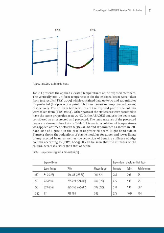
41Proceedings of the METNET Seminar 2011 in Aarhus
rectangle (Clauses 3.17 and 3.18 of [EN 1992-1-1, 2004]) stress-strain relationship was applied for compression and a bi-linear one for tension. Both of them were considered as ideally plastic. Maximum compressive and tensile stresses for concrete at 20 oC were 40 and 4 N/mm2, respectively and at elevated temperatures they were reduced according to [EN 1992-1-2, 2004]. All material models were inputted to ABAQUS every 100 oC and linear interpolation was used between those values. For simplicity, the surface between concrete and steel tube was modelled using TIE keyword meaning that the geometry performs exactly as if it was made of one piece. Two other beams and the middle column were modelled using beam elements. Modelling of concrete structures is demanding task and therefore the column model was validated by comparing the bending moment resistance of the column to those given for corresponding column in [TRY, 2004]. The bending resistance at ambient temperature from FEM was 6 % lower than that from [TRY, 2004] when material factors were 1.0. The connection between beam and column was modeled using rigid beam elements with a joint with a desired rotational stiffness between them (see also Fig. 3).
Figure 3. ABAQUS-model of the frame.
Table 1 presents the applied elevated temperatures of the exposed members. The vertically non-uniform temperatures for the exposed beam were taken from test results [TRY, 2009] which contained data up to 90 and 120 minutes for protected (fire protection paint in bottom flange) and unprotected beams, respectively. The uniform temperatures of the exposed part of the column were taken from [TRY, 2004]. Other parts of the structures were assumed to have the same properties as at 20 oC. In the ABAQUS analysis the beam was considered as unprotected and protected. The temperatures of the protected beam are shown in brackets in Table 1. Linear interpolation of temperatures was applied at times between 0, 30, 60, 90 and 120 minutes as shown in left-hand side of Figure 4 in the case of unprotected beam. Right-hand side of Figure 4 shows the reductions of elastic modulus for upper and lower flange of unprotected beam as well as the reduction of bending stiffness of edge column according to [TRY, 2004]. It can be seen that the stiffness of the column decreases faster than that of beam.
Table 1. Temperatures applied in the analysis [oC]. Exposed beam Exposed part of column (first floor) Lower flange Web Upper flange Concrete Tube Reinforcement
R30 546 (327) 546-88 (327-50) 101 (52) 260 705 95 R60 735 (524) 735-223 (524-115) 246 (122) 415 903 251 R90 829 (656) 829-358 (656-202) 392 (216) 510 987 387 R120 911 911-488 533 575 1037 494
Figure 3. ABAQUS-model of the frame.
Table 1 presents the applied elevated temperatures of the exposed members. The vertically non-uniform temperatures for the exposed beam were taken from test results [TRY, 2009] which contained data up to 90 and 120 minutes for protected (fire protection paint in bottom flange) and unprotected beams, respectively. The uniform temperatures of the exposed part of the column were taken from [TRY, 2004]. Other parts of the structures were assumed to have the same properties as at 20 oC. In the ABAQUS analysis the beam was considered as unprotected and protected. The temperatures of the protected beam are shown in brackets in Table 1. Linear interpolation of temperatures was applied at times between 0, 30, 60, 90 and 120 minutes as shown in left-hand side of Figure 4 in the case of unprotected beam. Right-hand side of Figure 4 shows the reductions of elastic modulus for upper and lower flange of unprotected beam as well as the reduction of bending stiffness of edge column according to [TRY, 2004]. It can be seen that the stiffness of the column decreases faster than that of beam.
Table 1. Temperatures applied in the analysis [oC].
Exposed beam Exposed part of column (first floor)
Lower flange Web Upper flange Concrete Tube Reinforcement
R30 546 (327) 546-88 (327-50) 101 (52) 260 705 95
R60 735 (524) 735-223 (524-115) 246 (122) 415 903 251
R90 829 (656) 829-358 (656-202) 392 (216) 510 987 387
R120 911 911-488 533 575 1037 494
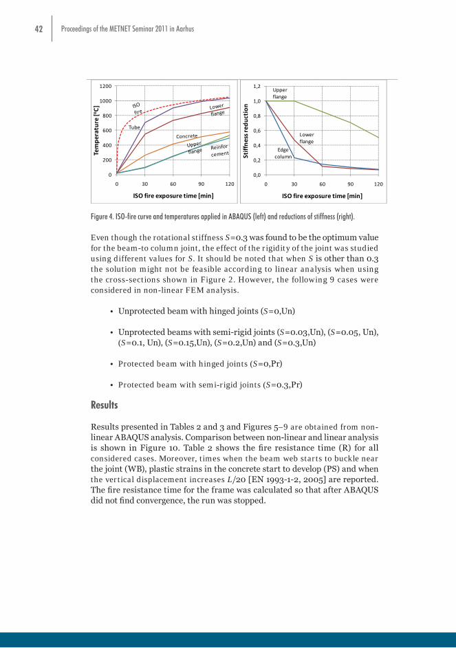
42 Proceedings of the METNET Seminar 2011 in Aarhus
R60 735 (524) 735-223 (524-115) 246 (122) 415 903 251 R90 829 (656) 829-358 (656-202) 392 (216) 510 987 387 R120 911 911-488 533 575 1037 494
Tube
0
200
400
600
800
1000
1200
0 30 60 90 120
Tempe
rature [oC]
ISO fire exposure time [min]
Lower flange
Upper flange
Edge column
0,0
0,2
0,4
0,6
0,8
1,0
1,2
0 30 60 90 120
Stiffne
ss re
duction
ISO fire exposure time [min]
Figure 4. ISO-fire curve and temperatures applied in ABAQUS (left) and reductions of stiffness (right).
Even though the rotational stiffness S=0.3 was found to be the optimum value for the beam-to column joint, the effect of the rigidity of the joint was studied using different values for S. It should be noted that when S is other than 0.3 the solution might not be feasible according to linear analysis when using the cross-sections shown in Figure 2. However, the following 9 cases were considered in non-linear FEM analysis.
- Unprotected beam with hinged joints (S=0,Un) - Unprotected beams with semi-rigid joints (S=0.03,Un), (S=0.05, Un), (S=0.1, Un), (S=0.15,Un), (S=0.2,Un) and (S=0.3,Un) - Protected beam with hinged joints (S=0,Pr) - Protected beam with semi-rigid joints (S=0.3,Pr)
Results Results presented in Tables 2 and 3 and Figures 59 are obtained from non-linear ABAQUS analysis. Comparison between non-linear and linear analysis is shown in Figure 10. Table 2 shows the fire resistance time (R) for all considered cases. Moreover, times when the beam web starts to buckle near the joint (WB), plastic strains in the concrete start to develop (PS) and when the vertical displacement increases L/20 [EN 1993-1-2, 2005] are reported. The fire resistance time for the frame was calculated so that after ABAQUS did not find convergence, the run was stopped.
Table 2. Fire resistance times and failures. Case S=0,
Un S=0.03,
Un S=0.05,
Un S=0.1,
Un S=0.15,
Un S=0.2,
Un S=0.3,
Un S=0, Pr
S=0.3, Pr
R [min] 54 59 75 72 67 64 60 83 ≥90 WB starts [min] - - 57 42 36 30 24 - 51 PS1 starts [min] 27 30 42 54 54 53 52 43 21* PS2 starts [min] 36 50 71 72 - - - 72 21*
Failure in Col. Col. Beam Beam Beam Beam Col. - L/20 at [min] 28 32 38 51 55 57 59 57 ≥90
Figure 4. ISO-fire curve and temperatures applied in ABAQUS (left) and reductions of stiffness (right).
Even though the rotational stiffness S=0.3 was found to be the optimum value for the beam-to column joint, the effect of the rigidity of the joint was studied using different values for S. It should be noted that when S is other than 0.3 the solution might not be feasible according to linear analysis when using the cross-sections shown in Figure 2. However, the following 9 cases were considered in non-linear FEM analysis.
• Unprotected beam with hinged joints (S=0,Un)
• Unprotected beams with semi-rigid joints (S=0.03,Un), (S=0.05, Un), (S=0.1, Un), (S=0.15,Un), (S=0.2,Un) and (S=0.3,Un)
• Protected beam with hinged joints (S=0,Pr)
• Protected beam with semi-rigid joints (S=0.3,Pr)
Results
Results presented in Tables 2 and 3 and Figures 5-9 are obtained from non-linear ABAQUS analysis. Comparison between non-linear and linear analysis is shown in Figure 10. Table 2 shows the fire resistance time (R) for all considered cases. Moreover, times when the beam web starts to buckle near the joint (WB), plastic strains in the concrete start to develop (PS) and when the vertical displacement increases L/20 [EN 1993-1-2, 2005] are reported. The fire resistance time for the frame was calculated so that after ABAQUS did not find convergence, the run was stopped.

43Proceedings of the METNET Seminar 2011 in Aarhus
Table 2. Fire resistance times and failures.
Case
S=0,
Un
S=0.03,
Un
S=0.05,Un S=0.1,
Un
S=0.15,
Un
S=0.2,
Un
S=0.3,
Un
S=0,
Pr
S=0.3,
Pr
R [min] 54 59 75 72 67 64 60 83 ≥90
WB starts [min] - - 57 42 36 30 24 - 51
PS1 starts [min] 27 30 42 54 54 53 52 43 21*
PS2 starts [min] 36 50 71 72 - - - 72 21*
Failure in Col. Col. Beam Beam Beam Beam Col. -
L/20 at [min] 28 32 38 51 55 57 59 57 ≥90
WB = web buckling
PS = Plastic strains in the concrete start to develop, 1=at floor level 2=at first beam level
* bending moments on the different direction than in all other cases
In the cases of hinged or very small rotational stiffness of the joint (S=0,Un; S=0.03,Un and S=0,Pr) the failure of the frame occurred due to the plastic hinges of the column. In the cases of relatively high rotational stiffness of the joint (S=0.1,Un; S=0.15,Un; S=0.2,Un and S=0.3,Un) the failure occurred due to web buckling of the beam. In the case S=0.05,Un both web buckling in beam and plastic hinges in column were noticed. Case S=0.3,Pr resisted to the whole calculation up to 90 minutes without failure. Slight plastification in the concrete was observed due to thermal expansion after 21 minutes. However, after that, the catenary action started to take place and no further damage occurred. Figure 5 shows the results of Table 2 for unprotected beams as a function of the rotational stiffness of the joint.
WB = web buckling PS = Plastic strains in the concrete start to develop, 1=at floor level 2=at first beam level * bending moments on the different direction than in all other cases In the cases of hinged or very small rotational stiffness of the joint (S=0,Un; S=0.03,Un and S=0,Pr) the failure of the frame occurred due to the plastic hinges of the column. In the cases of relatively high rotational stiffness of the joint (S=0.1,Un; S=0.15,Un; S=0.2,Un and S=0.3,Un) the failure occurred due to web buckling of the beam. In the case S=0.05,Un both web buckling in beam and plastic hinges in column were noticed. Case S=0.3,Pr resisted to the whole calculation up to 90 minutes without failure. Slight plastification in the concrete was observed due to thermal expansion after 21 minutes. However, after that, the catenary action started to take place and no further damage occurred. Figure 5 shows the results of Table 2 for unprotected beams as a function of the rotational stiffness of the joint.
Failure in columnFailure in beam
web
Fire resistance time
Web buckling starts
PS1 startsPS2 starts
0
30
60
90
0,00 0,10 0,20 0,30
ISO fire exp
osure time [m
in]
S Figure 5. Fire resistance times and failures as a function of S.
Table 2 and Figure 5 reveal that when the beam was unprotected and S varied from 0 to 0.3, the frame resisted, on average, 64 minutes of ISO fire. The value S=0.05 seemed to be approximately the optimum stiffness to get the highest fire resistance time (75 min) for the considered frame with the unprotected beam. Joints with smaller stiffness leaded to earlier failure in the column and more rigid joints yielded to earlier buckling of the beam web. Figure 6 shows the maximum vertical displacement of the exposed beam and horizontal displacements (positive values inwards the building) of the column at the first floor. The vertical deflection limits L/20 = 582 mm [EN 1993-1-2, 2005] and L2/400h = 989 mm (≈ L/12 in this case) [Twilt, 2002], where h is the height of the beam, are also drawn. It should be noted that in reality, the horizontal displacements of the column would be resisted by the concrete slab, also.
S=0,Un
S=0,Pr
S=0.3,Un
S=0.3,Pr
S=0.03,Un S=0.05,Un
S=0.1,UnS=0.15,Un
S=0.2,Un
L/20
L2/400h
‐1400
‐1200
‐1000
‐800
‐600
‐400
‐200
0
0 30 60 90
Vertical displacem
ent [mm]
ISO fire exposure time [min]
Unprotected beam
Protected beam
S=0,Un
S=0,Pr
S=0.3,UnS=0.3,Pr
S=0.1,UnS=0.05,Un
S=0.03,Un
S=0.15,UnS=0.2,Un
‐50
0
50
100
150
200
250
0 30 60 90Horizon
tal d
isplacem
ent [mm]
ISO fire exposure time [min]
Unprotected beam
Protected beam
Figure 5. Fire resistance times and failures as a function of S.

44 Proceedings of the METNET Seminar 2011 in Aarhus
Table 2 and Figure 5 reveal that when the beam was unprotected and S varied from 0 to 0.3, the frame resisted, on average, 64 minutes of ISO fire. The value S=0.05 seemed to be approximately the optimum stiffness to get the highest fire resistance time (75 min) for the considered frame with the unprotected beam. Joints with smaller stiffness leaded to earlier failure in the column and more rigid joints yielded to earlier buckling of the beam web. Figure 6 shows the maximum vertical displacement of the exposed beam and horizontal displacements (positive values inwards the building) of the column at the first floor. The vertical deflection limits L/20 = 582 mm [EN 1993-1-2, 2005] and L2/400h = 989 mm (≈ L/12 in this case) [Twilt, 2002], where h is the height of the beam, are also drawn. It should be noted that in reality, the horizontal displacements of the column would be resisted by the concrete slab, also.
WB = web buckling PS = Plastic strains in the concrete start to develop, 1=at floor level 2=at first beam level * bending moments on the different direction than in all other cases In the cases of hinged or very small rotational stiffness of the joint (S=0,Un; S=0.03,Un and S=0,Pr) the failure of the frame occurred due to the plastic hinges of the column. In the cases of relatively high rotational stiffness of the joint (S=0.1,Un; S=0.15,Un; S=0.2,Un and S=0.3,Un) the failure occurred due to web buckling of the beam. In the case S=0.05,Un both web buckling in beam and plastic hinges in column were noticed. Case S=0.3,Pr resisted to the whole calculation up to 90 minutes without failure. Slight plastification in the concrete was observed due to thermal expansion after 21 minutes. However, after that, the catenary action started to take place and no further damage occurred. Figure 5 shows the results of Table 2 for unprotected beams as a function of the rotational stiffness of the joint.
Failure in columnFailure in beam
web
Fire resistance time
Web buckling starts
PS1 startsPS2 starts
0
30
60
90
0,00 0,10 0,20 0,30
ISO fire exp
osure time [m
in]
S Figure 5. Fire resistance times and failures as a function of S.
Table 2 and Figure 5 reveal that when the beam was unprotected and S varied from 0 to 0.3, the frame resisted, on average, 64 minutes of ISO fire. The value S=0.05 seemed to be approximately the optimum stiffness to get the highest fire resistance time (75 min) for the considered frame with the unprotected beam. Joints with smaller stiffness leaded to earlier failure in the column and more rigid joints yielded to earlier buckling of the beam web. Figure 6 shows the maximum vertical displacement of the exposed beam and horizontal displacements (positive values inwards the building) of the column at the first floor. The vertical deflection limits L/20 = 582 mm [EN 1993-1-2, 2005] and L2/400h = 989 mm (≈ L/12 in this case) [Twilt, 2002], where h is the height of the beam, are also drawn. It should be noted that in reality, the horizontal displacements of the column would be resisted by the concrete slab, also.
S=0,Un
S=0,Pr
S=0.3,Un
S=0.3,Pr
S=0.03,Un S=0.05,Un
S=0.1,UnS=0.15,Un
S=0.2,Un
L/20
L2/400h
‐1400
‐1200
‐1000
‐800
‐600
‐400
‐200
0
0 30 60 90
Vertical displacem
ent [mm]
ISO fire exposure time [min]
Unprotected beam
Protected beam
S=0,Un
S=0,Pr
S=0.3,UnS=0.3,Pr
S=0.1,UnS=0.05,Un
S=0.03,Un
S=0.15,UnS=0.2,Un
‐50
0
50
100
150
200
250
0 30 60 90Horizon
tal d
isplacem
ent [mm]
ISO fire exposure time [min]
Unprotected beam
Protected beam
Figure 6. Vertical displacements of the beam (left) and horizontal displacements of the column at first floor (right).
Figure 7 presents the horizontal forces in the heated beam for cases S=0,Un; S=0.03,Un; S=0.05,Un; S=0.15,Un; S=0.3,Un; S=0,Pr and S=0.3,Pr. The horizontal forces in cases S=0.1,Un and S=0.2,Un were between those of S=0.15,Un and S=0.3,Un. Tie force 430 kN according to EN 1991-1-7 [EN 1991-1-7, 2006] is drawn also in Figure 7. Table 3 lists the minimum (compression) and maximum (tension) values of horizontal forces in beam in all considered cases. The times when the minimum values were observed, are also reported. All the maximum values occurred at the end of the analysis.
S=0,UnS=0.03,Un S=0.05,Un
S=0,Pr
S=0.3,Pr
EN 1991‐1‐7 Tie force
‐150
‐50
50
150
250
350
450
0 30 60 90
Horizon
tal force [k
N]
ISO fire exposure time [min]
S=0,UnS=0.03,UnS=0.05,UnS=0.15,UnS=0.3,UnS=0,PrS=0.3,Pr
Figure 7. Horizontal forces of exposed beam.
The horizontal force in unprotected exposed beam reaches its minimum value around 12 minutes. After that, the compression in beam changes to tension around 15 to 25 minutes and increases till the end of analysis due to catenary action. The rigidity of the joint increases the maximum compressive forces and decreases the maximum tensile forces in the beam. The tensile capacity of the beam is not exceeded at any time. At 90 minutes the capacity is still approximately 4300 kN. In all cases, the maximum tensile force is lower than the tie force according to EN 1991-1-7 [EN 1991-1-7, 2006]. Figure 8 shows the displacement profiles of the left column in cases S=0,Un and S=0.3,Un at different times. The scaling factor in both cases is 30.
Figure 8. Displacement profiles for edge column at different times in cases S=0,Un and S=0.3,Un (scaling
factor 30). Figures 68 reveal that the behaviour of the frame in fire depends significantly on the stiffness of the joint. The rigidity of the joint decreases the vertical displacements of the
Figure 7. Horizontal forces of exposed beam.

45Proceedings of the METNET Seminar 2011 in Aarhus
The horizontal force in unprotected exposed beam reaches its minimum value around 12 minutes. After that, the compression in beam changes to tension around 15 to 25 minutes and increases till the end of analysis due to catenary action. The rigidity of the joint increases the maximum compressive forces and decreases the maximum tensile forces in the beam. The tensile capacity of the beam is not exceeded at any time. At 90 minutes the capacity is still approximately 4300 kN. In all cases, the maximum tensile force is lower than the tie force according to EN 1991-1-7 [EN 1991-1-7, 2006]. Figure 8 shows the displacement profiles of the left column in cases S=0,Un and S=0.3,Un at different times. The scaling factor in both cases is 30.
Figure 6. Vertical displacements of the beam (left) and horizontal displacements of the column at first floor (right).
Figure 7 presents the horizontal forces in the heated beam for cases S=0,Un; S=0.03,Un; S=0.05,Un; S=0.15,Un; S=0.3,Un; S=0,Pr and S=0.3,Pr. The horizontal forces in cases S=0.1,Un and S=0.2,Un were between those of S=0.15,Un and S=0.3,Un. Tie force 430 kN according to EN 1991-1-7 [EN 1991-1-7, 2006] is drawn also in Figure 7. Table 3 lists the minimum (compression) and maximum (tension) values of horizontal forces in beam in all considered cases. The times when the minimum values were observed, are also reported. All the maximum values occurred at the end of the analysis.
S=0,UnS=0.03,Un S=0.05,Un
S=0,Pr
S=0.3,Pr
EN 1991‐1‐7 Tie force
‐150
‐50
50
150
250
350
450
0 30 60 90
Horizon
tal force [k
N]
ISO fire exposure time [min]
S=0,UnS=0.03,UnS=0.05,UnS=0.15,UnS=0.3,UnS=0,PrS=0.3,Pr
Figure 7. Horizontal forces of exposed beam.
The horizontal force in unprotected exposed beam reaches its minimum value around 12 minutes. After that, the compression in beam changes to tension around 15 to 25 minutes and increases till the end of analysis due to catenary action. The rigidity of the joint increases the maximum compressive forces and decreases the maximum tensile forces in the beam. The tensile capacity of the beam is not exceeded at any time. At 90 minutes the capacity is still approximately 4300 kN. In all cases, the maximum tensile force is lower than the tie force according to EN 1991-1-7 [EN 1991-1-7, 2006]. Figure 8 shows the displacement profiles of the left column in cases S=0,Un and S=0.3,Un at different times. The scaling factor in both cases is 30.
Figure 8. Displacement profiles for edge column at different times in cases S=0,Un and S=0.3,Un (scaling
factor 30). Figures 68 reveal that the behaviour of the frame in fire depends significantly on the stiffness of the joint. The rigidity of the joint decreases the vertical displacements of the
Figure 8. Displacement profiles for edge column at different times in cases S=0,Un and S=0.3,Un (scaling factor 30).
Figures 6-8 reveal that the behaviour of the frame in fire depends significantly on the stiffness of the joint. The rigidity of the joint decreases the vertical displacements of the beam and horizontal displacements of the column clearly. The disadvantage of the increased S is the web buckling which occurs near the joint due to negative moment which produces compression on the lower (hotter) part of the beam web. Figure 9 illustrates the web buckling at different times in the case S=0.3,Un. Table 2 shows that after the first buckles were observed, the beam could resist still a rather long time. In reality, the lower flange of the beam supports the concrete slabs which would prevent the web buckling outwards of the cross-section.
beam and horizontal displacements of the column clearly. The disadvantage of the increased S is the web buckling which occurs near the joint due to negative moment which produces compression on the lower (hotter) part of the beam web. Figure 9 illustrates the web buckling at different times in the case S=0.3,Un. Table 2 shows that after the first buckles were observed, the beam could resist still a rather long time. In reality, the lower flange of the beam supports the concrete slabs which would prevent the web buckling outwards of the cross-section.
Figure 9. Buckling of beam web in the case S=0.3,Un (scaling factor 3).
Table 3 shows the maximum strains in the lower flange of the beam as a function of ISO fire exposure time. The motivation for this comes from the maximum strain of the fire protection material, which is typically approximately 2 %.
Table 3. Maximum strains [%] in lower flange at different times and temperatures. Case S=0,
Un S=0.03,
Un S=0.05,
Un S=0.1,
Un S=0.15,
Un S=0.2,
Un S=0.3,
Un S=0, Pr
S=0.3, Pr
R0 0.14 0.14 0.13 0.13 0.12 0.12 0.11 0.14 0.11 R30 1.54 1.26 1.12 0.94 0.87 0.83 0.79 0.70 0.48 R60 - - 2.48 2.13 2.00 1.93 1.87 1.49 0.76 R90 - - - - - - - - 1.14 Rmax [min]
3.74 54
2.72 59
3.21 75
2.72 72
2.34 67
2.13 64
1.89 60
2.90 83
- -
Tlf,crit [oC] 596 645 672 721 735 740 - 571 - The maximum strain of protected and hinged beam (S=0,Pr) exceeded 2 % at approximately 71 minutes. In the case S=0.3,Pr, the maximum strain was 1.14 % at the end of the calculation (90 minutes). The effect of joint rigidity has a major effect on the strain of the beam. The same conclusion can be drawn also from the results of unprotected beams. In the case S=0,Un, the 2 % strain was exceeded at lower flange temperature 596 oC. When the joint stiffness S was at least 0.1, the corresponding lower flange temperatures were at least 721 oC. Figure 10 presents a comparison between ABAQUS-analysis and typical linear design procedure for case S=0.3,Un at times 0, 30 and 60 minutes. Bending moment distribution and shear force at the floor level for the edge column are considered.
Figure 9. Buckling of beam web in the case S=0.3,Un (scaling factor 3).
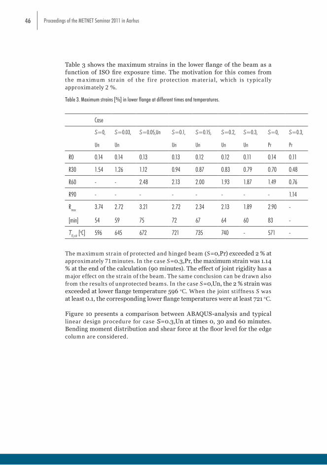
46 Proceedings of the METNET Seminar 2011 in Aarhus
Table 3 shows the maximum strains in the lower flange of the beam as a function of ISO fire exposure time. The motivation for this comes from the maximum strain of the fire protection material, which is typically approximately 2 %.
Table 3. Maximum strains [%] in lower flange at different times and temperatures.
Case
S=0,
Un
S=0.03,
Un
S=0.05,Un S=0.1,
Un
S=0.15,
Un
S=0.2,
Un
S=0.3,
Un
S=0,
Pr
S=0.3,
Pr
R0 0.14 0.14 0.13 0.13 0.12 0.12 0.11 0.14 0.11
R30 1.54 1.26 1.12 0.94 0.87 0.83 0.79 0.70 0.48
R60 - - 2.48 2.13 2.00 1.93 1.87 1.49 0.76
R90 - - - - - - - - 1.14
Rmax
[min]
3.74
54
2.72
59
3.21
75
2.72
72
2.34
67
2.13
64
1.89
60
2.90
83
-
-
Tlf,crit [oC] 596 645 672 721 735 740 - 571 -
The maximum strain of protected and hinged beam (S=0,Pr) exceeded 2 % at approximately 71 minutes. In the case S=0.3,Pr, the maximum strain was 1.14 % at the end of the calculation (90 minutes). The effect of joint rigidity has a major effect on the strain of the beam. The same conclusion can be drawn also from the results of unprotected beams. In the case S=0,Un, the 2 % strain was exceeded at lower flange temperature 596 oC. When the joint stiffness S was at least 0.1, the corresponding lower flange temperatures were at least 721 oC.
Figure 10 presents a comparison between ABAQUS-analysis and typical linear design procedure for case S=0.3,Un at times 0, 30 and 60 minutes. Bending moment distribution and shear force at the floor level for the edge column are considered.
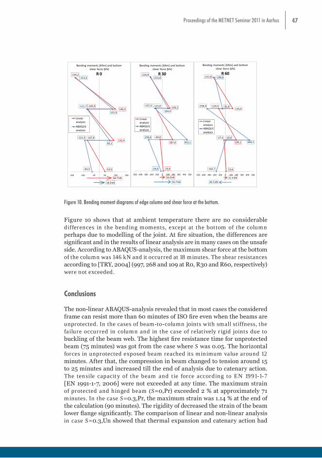
47Proceedings of the METNET Seminar 2011 in Aarhus
53,0
‐107,8132,4
‐105,9146,3
‐220,2
44.7 kN
‐64,3
‐131,3
95,1
‐111,7
121,9
‐213,2
18.9 kN
‐250 ‐150 ‐50 50 150 250
Bending moments [kNm] and bottom shear force [kN]
R 0
Linear analysis
ABAQUS analysis
19,9
‐40,0
187,6
‐121,0136,2
‐220,8
16.6 kN
‐24,6
‐250,6
452,1
‐137,3
104,4
‐213,0
59.7 kN
‐500 ‐400 ‐300 ‐200 ‐100 0 100 200 300 400 500
Bending moments [kNm] and bottom shear force [kN]
R 30
Linear analysisABAQUS analysis
13,6
‐27,4
199,1
‐124,5135,0
‐221,8
11.4 kN
‐165,7
10,0
440,1
‐336,9 ‐55,8
‐196,6
44.1 kN
‐500 ‐400 ‐300 ‐200 ‐100 0 100 200 300 400 500
Bending moments [kNm] and bottom shear force [kN]
R 60
Linear analysisABAQUS analysis
Figure 10. Bending moment diagrams of edge column and shear force at the bottom.
Figure 10 shows that at ambient temperature there are no considerable differences in the bending moments, except at the bottom of the column perhaps due to modelling of the joint. At fire situation, the differences are significant and in the results of linear analysis are in many cases on the unsafe side. According to ABAQUS-analysis, the maximum shear force at the bottom of the column was 146 kN and it occurred at 18 minutes. The shear resistances according to [TRY, 2004] (997, 268 and 109 at R0, R30 and R60, respectively) were not exceeded. Conclusions The non-linear ABAQUS-analysis revealed that in most cases the considered frame can resist more than 60 minutes of ISO fire even when the beams are unprotected. In the cases of beam-to-column joints with small stiffness, the failure occurred in column and in the case of relatively rigid joints due to buckling of the beam web. The highest fire resistance time for unprotected beam (75 minutes) was got from the case where S was 0.05. The horizontal forces in unprotected exposed beam reached its minimum value around 12 minutes. After that, the compression in beam changed to tension around 15 to 25 minutes and increased till the end of analysis due to catenary action. The tensile capacity of the beam and tie force according to EN 1991-1-7 [EN 1991-1-7, 2006] were not exceeded at any time. The maximum strain of protected and hinged beam (S=0,Pr) exceeded 2 % at approximately 71 minutes. In the case S=0.3,Pr, the maximum strain was 1.14 % at the end of the calculation (90 minutes). The rigidity of decreased the strain of the beam lower flange significantly. The comparison of linear and non-linear analysis in case S=0.3,Un showed that thermal expansion and catenary action had a significant effect on the column bending moments and shear force in fire situation. In further researches more cases will be covered in comparison.
Figure 10. Bending moment diagrams of edge column and shear force at the bottom.
Figure 10 shows that at ambient temperature there are no considerable differences in the bending moments, except at the bottom of the column perhaps due to modelling of the joint. At fire situation, the differences are significant and in the results of linear analysis are in many cases on the unsafe side. According to ABAQUS-analysis, the maximum shear force at the bottom of the column was 146 kN and it occurred at 18 minutes. The shear resistances according to [TRY, 2004] (997, 268 and 109 at R0, R30 and R60, respectively) were not exceeded.
Conclusions
The non-linear ABAQUS-analysis revealed that in most cases the considered frame can resist more than 60 minutes of ISO fire even when the beams are unprotected. In the cases of beam-to-column joints with small stiffness, the failure occurred in column and in the case of relatively rigid joints due to buckling of the beam web. The highest fire resistance time for unprotected beam (75 minutes) was got from the case where S was 0.05. The horizontal forces in unprotected exposed beam reached its minimum value around 12 minutes. After that, the compression in beam changed to tension around 15 to 25 minutes and increased till the end of analysis due to catenary action. The tensile capacity of the beam and tie force according to EN 1991-1-7 [EN 1991-1-7, 2006] were not exceeded at any time. The maximum strain of protected and hinged beam (S=0,Pr) exceeded 2 % at approximately 71 minutes. In the case S=0.3,Pr, the maximum strain was 1.14 % at the end of the calculation (90 minutes). The rigidity of decreased the strain of the beam lower flange significantly. The comparison of linear and non-linear analysis in case S=0.3,Un showed that thermal expansion and catenary action had
48 Proceedings of the METNET Seminar 2011 in Aarhus
a significant effect on the column bending moments and shear force in fire situation. In further researches more cases will be covered in comparison.
References
ABAQUS 6.10/CAE User’s Manual, Dassault Systemes, 2010
EN 1991-1-2, Eurocode 1: Actions on structures – Part 1-2: General actions – Actions on structures exposed to fire, CEN, Brussels, 2002
EN 1991-1-7, Eurocode 1: Actions on structures – Part 1-7: General actions – Accidenta actions, CEN, Brussels, 2006
EN 1992-1-1, Eurocode 2: Design of concrete structures – Part 1-1: General rules and rules for buildings, CEN, Brussels, 2004
EN 1992-1-2, Eurocode 2: Design of concrete structures – Part 1-2: General rules – Structural fire design, CEN, Brussels, 2004
EN 1993-1-1, Eurocode 3: Design of steel structures – Part 1-1: General rules and rules for buildings, CEN, Brussels, 2005
EN 1993-1-2, Eurocode 3: Design of steel structures – Part 1-2: General rules. Structural fire design, CEN, Brussels, 2005
EN 1993-1-5, Eurocode 3: Design of steel structures – Part 1-5: Plated structural elements, CEN, Brussels, 2005
EN 1994-1-2, Eurocode 4: Design of composite steel and concrete structures – Part 1-2: General rules – Structural fire design, CEN, Brussels, 2005
Jalkanen J., Tubular Truss Optimization Using Heuristic Algorithms, Doctoral Thesis, Tampere University of Technology, Publication 706, Tampere, 2007
Matlab® ver. 7.8.0.347 (R2009a), The MathWorks™, 2009
Monforton G.R., Wu T.S., Matrix analysis of semi-rigidly connected frames, Journal of Structural Division, V.89, N.6, 1963
TRY, Teräsnormikortti N:o 21/2009, WQ-palkin poikkileikkauksen mitoitus normaali- ja palotilanteessa (In Finnish), TRY, 2009
TRY, Betonitäytteisen teräsliittopilarin suunnitteluohje (In Finnish), Julkaisumonistamo Eteläranta Oy, Helsinki, 2004
Twilt L., Design tools for the behaviour of multi-storey steel framed buildings exposed to natural fires, 8th interim report, TNO report, TNO, 2002

49Proceedings of the METNET Seminar 2011 in Aarhus
Wald F., Simões da Silva L., Moore D.B., Lennon T., Chladna M., Santiago A., Benes M., Borges L., Experimental behaviour of a steel structure under natural fire, Fire Safety Journal 41, 2006, pp. 509-522
Wald F., Kallerova P., Chlouba J., Sokol Z., Strejcek M., Pospisil J., Stroner M., Kremen T., Smitka V., Fire Test on an Administrative Building in Mokrsko, Printing house Ceska technika, Czech Technical University in Prague, 2010
Yin Y.Z., Wang Y.C., A numerical study of large deflection behaviour of restrained steel beams at elevated temperatures, Journal of Constructional Steel Research 60, 2004, pp. 1029-1047
Yin Y.Z., Wang Y.C., Analysis of catenary action in steel beams using a simplified hand calculation method, Part 1: theory and validation for non-uniform temperature distribution, Journal of Constructional Steel Research 61, 2005, pp. 183-211
50 Proceedings of the METNET Seminar 2011 in Aarhus
EFFECT OF ZINC COATING ON STEEL TEMPERATURES AT ELEVATED TEMPERATURES
Keijo Fränti
Hilkka Ronni
Markku Heinisuo
Tampere University of Technology
Research Centre of Metal Structures
Abstract
Hot dip zinc i.e., galvanized, coatings are often used as corrosion protection for steel structures located outside or under severe climate classes. Because galvanized coating is mainly applied for corrosion protection purposes, most of the studies on galvanized steel structures have concentrated on their corrosion performance. Recent studies (Jutila, 2010), (Jirku, 2011) have indicated that galvanized coating may also contribute positively to the fire protection performance of steel.
In this paper the main test results of (Jutila, 2010) are given. The observed time lag for rising of steel temperature due to galvanizing is modeled by lowering the emissivity of the galvanized steel surface below 420 oC and corresponding steel temperatures are shown. The comparisons of steel temperatures with zinc and without zinc are given at elevated temperatures for standard ISO fire applying equations of Eurocodes (EN 1993-1-2, 2005).
Tests with galvanized steel at elevated temperatures
Preliminary studies (Jutila, 2010; Jirku, 2011) have shown that the temperatures of galvanized steel members are lower than those of corresponding uncoated steel members when exposed to elevated temperatures. Tests in (Jutila, 2010) were done using the cone calorimeter and test in (Jirku, 2011) were done using furnace. The results were well in line. In this paper test results of (Jutila, 2010) are shown briefly.
Tests by Jutila (Jutila, 2010) employed steel S235JRG2 specimens of the size of 100x100x2 mm3 as galvanized with three zinc thicknesses and uncoated and were done using a cone calorimeter and heat fluxes of 25, 50 and 75 kW/m2. The heat flux was applied as long as temperature of the specimen changed. The results showed that by using the lowest heat flux 25 kW/m2 temperature of the galvanized specimens remained 250oC, lower than that of uncoated counterparts all through the test. By using higher heat fluxes, temperature of the galvanized specimens increased with increase in heating time but reached

51Proceedings of the METNET Seminar 2011 in Aarhus
that of uncoated steel only after a time lag of several minutes. Table 1 presents the composition of steel plates used in tests.
Table 1. Composition of steel plates.
Element C Mn Si S P Cr Ni Cu As N
% 0.15 0.33 0.02 0.031 0.013 0.05 0.04 0.06 0.08 0.008
Table 2 presents the measured zinc thicknesses of the samples. There were 3 samples of each zinc thicknesses.
Table 2. Measured zinc thicknesses with variations.
Coating Coating thickness Variation, µm
1 66 µm 1.3 (2 %)
2 86.3 µm 3.7 (4,3 %)
3 107.9 µm 14.7 (13,7 %)
When considering the results the following observations can be done:
• • Temperatures at top and bottom surfaces of the plates were about the same.
• • Variations in time-temperature relationships for heat fluxes 25 and 75 kW/m2 were small.
• • Variations in time-temperature relationships for the heat flux 50 kW/m2 were large with respect to time but small with respect to temperature.
Figures 1 and 2 and illustrate the results for heat fluxes 25 and 75 kW/m2. In figures are shown the results for uncoated plates, too.
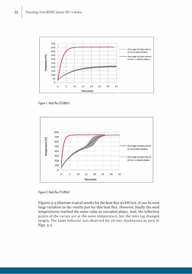
52 Proceedings of the METNET Seminar 2011 in Aarhus
0
50
100
150
200
250
300
350
400
450
500
0 5 10 15 20 25 30 35
Tempe
rature [°C]
Time [min]
Average temperature of uncoated plates
Average temperature of zinc coated plates
Figure 1. Heat flux 25 kW/m2.
0
100
200
300
400
500
600
700
800
0 5 10 15 20 25 30 35
Tempe
rature [°C]
Time [min]
Average temperature of uncoated plates
Average temperature of zinc coated plates
Figure 2. Heat flux 75 kW/m2.
Figures 3-5 illustrate typical results for the heat flux 50 kW/m2. It can be seen large variation in the results just for this heat flux. However, finally the steel temperatures reached the same value as uncoated plates. And, the inflection points of the curves are at the same temperature, but the time lag changed largely. The same behavior was observed for all zinc thicknesses as seen in Figs. 3-5.
Figure 1. Heat flux 25 kW/m2.
0
50
100
150
200
250
300
350
400
450
500
0 5 10 15 20 25 30 35
Tempe
rature [°C]
Time [min]
Average temperature of uncoated plates
Average temperature of zinc coated plates
Figure 1. Heat flux 25 kW/m2.
0
100
200
300
400
500
600
700
800
0 5 10 15 20 25 30 35
Tempe
rature [°C]
Time [min]
Average temperature of uncoated plates
Average temperature of zinc coated plates
Figure 2. Heat flux 75 kW/m2.
Figures 3-5 illustrate typical results for the heat flux 50 kW/m2. It can be seen large variation in the results just for this heat flux. However, finally the steel temperatures reached the same value as uncoated plates. And, the inflection points of the curves are at the same temperature, but the time lag changed largely. The same behavior was observed for all zinc thicknesses as seen in Figs. 3-5.
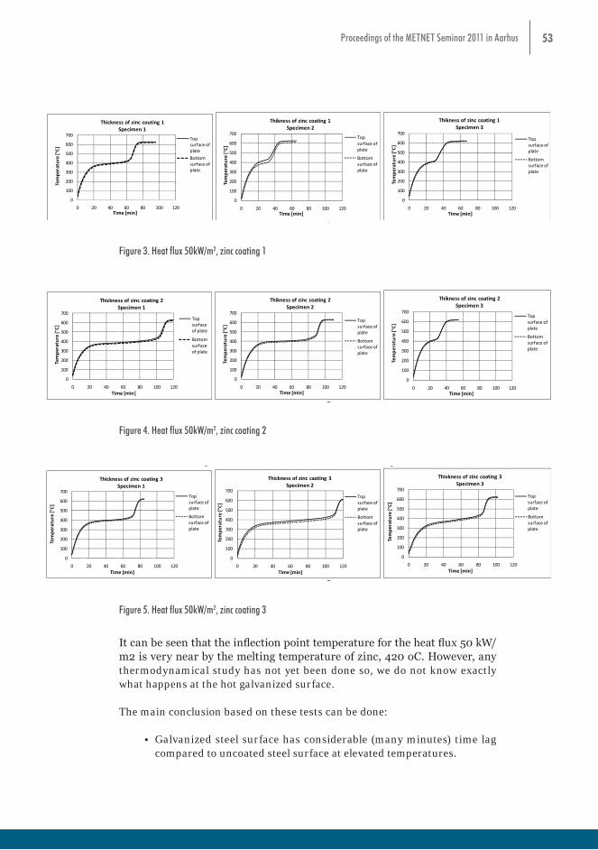
53Proceedings of the METNET Seminar 2011 in Aarhus
0
100
200
300
400
500
600
700
0 20 40 60 80 100 120
Tempe
rature [°C]
Time [min]
Thickness of zinc couting 1Specimen 1
Top surface of plate
Bottom surface of plate
0
100
200
300
400
500
600
700
0 20 40 60 80 100 120
Tempe
rature [°C]
Time [min]
Thikness of zinc coating 1Specimen 2
Top surface of plate
Bottom surface of plate
0
100
200
300
400
500
600
700
0 20 40 60 80 100 120
Tempe
rature [°C]
Time [min]
Thikness of zinc coating 1Specimen 3
Top surface of plate
Bottom surface of plate
Figure 3. Heat flux 50kW/m2, zinc coating 1
0
100
200
300
400
500
600
700
0 20 40 60 80 100 120
Tempe
rature [°C]
Time [min]
Thickness of zinc coating 2Specimen 1
Top surface of plate
Bottom surface of plate
0
100
200
300
400
500
600
700
0 20 40 60 80 100 120
Tempe
rature [°C]
Time [min]
Thikness of zinc coating 2Specimen 2
Top surface of plate
Bottom surface of plate
0
100
200
300
400
500
600
700
0 20 40 60 80 100 120
Tempe
rature [°C]
Time [min]
Thikness of zinc coating 2Specimen 3
Top surface of plate
Bottom surface of plate
Figure 4. Heat flux 50kW/m2, zinc coating 2
0
100
200
300
400
500
600
700
0 20 40 60 80 100 120
Tempe
rature [°C]
Time [min]
Thickness of zinc coating 3Specimen 1
Top surface of plate
Bottom surface of plate
0
100
200
300
400
500
600
700
0 20 40 60 80 100 120
Tempe
rature [°C]
Time [min]
Thickness of zinc caoting 3Specimen 2
Top surface of plate
Bottom surface of plate
0
100
200
300
400
500
600
700
0 20 40 60 80 100 120
Tempe
rature [°C]
Time [min]
Thivkness of zinc coating 3Specimen 3
Top surface of plate
Bottom surface of plate
Figure 5. Heat flux 50kW/m2, zinc coating 3
It can be seen that the inflection point temperature for the heat flux 50 kW/m2 is very near by the melting temperature of zinc, 420 oC. However, any thermodynamical study has not yet been done so, we do not know exactly what happens at the hot galvanized surface. The main conclusion based on these tests can be done:
Galvanized steel surface has considerable (many minutes) time lag compared to uncoated steel surface at elevated temperatures.
All thermomechanical features at elevated temperatures on galvanized steel surfaces MAY be compensated simply redusing the emissivity of the galvanized steel surface, as proposed in (Jutila, 2010), up to value 0.2 below 420 oC, then the analysis of galvanized steel structures is possible to perform, as shown in the following chapter. In (EN 1993-1-2, 2005) the value 0.7 is given for uncoated carbon steel. It should be noted that no theoretical basis for this assumption is not available. Estimation of resistance of galvanized steel structures in fire
Figure 3. Heat flux 50kW/m2, zinc coating 1
0
100
200
300
400
500
600
700
0 20 40 60 80 100 120
Tempe
rature [°C]
Time [min]
Thickness of zinc couting 1Specimen 1
Top surface of plate
Bottom surface of plate
0
100
200
300
400
500
600
700
0 20 40 60 80 100 120
Tempe
rature [°C]
Time [min]
Thikness of zinc coating 1Specimen 2
Top surface of plate
Bottom surface of plate
0
100
200
300
400
500
600
700
0 20 40 60 80 100 120
Tempe
rature [°C]
Time [min]
Thikness of zinc coating 1Specimen 3
Top surface of plate
Bottom surface of plate
Figure 3. Heat flux 50kW/m2, zinc coating 1
0
100
200
300
400
500
600
700
0 20 40 60 80 100 120
Tempe
rature [°C]
Time [min]
Thickness of zinc coating 2Specimen 1
Top surface of plate
Bottom surface of plate
0
100
200
300
400
500
600
700
0 20 40 60 80 100 120
Tempe
rature [°C]
Time [min]
Thikness of zinc coating 2Specimen 2
Top surface of plate
Bottom surface of plate
0
100
200
300
400
500
600
700
0 20 40 60 80 100 120Tempe
rature [°C]
Time [min]
Thikness of zinc coating 2Specimen 3
Top surface of plate
Bottom surface of plate
Figure 4. Heat flux 50kW/m2, zinc coating 2
0
100
200
300
400
500
600
700
0 20 40 60 80 100 120
Tempe
rature [°C]
Time [min]
Thickness of zinc coating 3Specimen 1
Top surface of plate
Bottom surface of plate
0
100
200
300
400
500
600
700
0 20 40 60 80 100 120
Tempe
rature [°C]
Time [min]
Thickness of zinc caoting 3Specimen 2
Top surface of plate
Bottom surface of plate
0
100
200
300
400
500
600
700
0 20 40 60 80 100 120
Tempe
rature [°C]
Time [min]
Thivkness of zinc coating 3Specimen 3
Top surface of plate
Bottom surface of plate
Figure 5. Heat flux 50kW/m2, zinc coating 3
It can be seen that the inflection point temperature for the heat flux 50 kW/m2 is very near by the melting temperature of zinc, 420 oC. However, any thermodynamical study has not yet been done so, we do not know exactly what happens at the hot galvanized surface. The main conclusion based on these tests can be done:
Galvanized steel surface has considerable (many minutes) time lag compared to uncoated steel surface at elevated temperatures.
All thermomechanical features at elevated temperatures on galvanized steel surfaces MAY be compensated simply redusing the emissivity of the galvanized steel surface, as proposed in (Jutila, 2010), up to value 0.2 below 420 oC, then the analysis of galvanized steel structures is possible to perform, as shown in the following chapter. In (EN 1993-1-2, 2005) the value 0.7 is given for uncoated carbon steel. It should be noted that no theoretical basis for this assumption is not available. Estimation of resistance of galvanized steel structures in fire
Figure 4. Heat flux 50kW/m2, zinc coating 2
0
100
200
300
400
500
600
700
0 20 40 60 80 100 120
Tempe
rature [°C]
Time [min]
Thickness of zinc couting 1Specimen 1
Top surface of plate
Bottom surface of plate
0
100
200
300
400
500
600
700
0 20 40 60 80 100 120
Tempe
rature [°C]
Time [min]
Thikness of zinc coating 1Specimen 2
Top surface of plate
Bottom surface of plate
0
100
200
300
400
500
600
700
0 20 40 60 80 100 120
Tempe
rature [°C]
Time [min]
Thikness of zinc coating 1Specimen 3
Top surface of plate
Bottom surface of plate
Figure 3. Heat flux 50kW/m2, zinc coating 1
0
100
200
300
400
500
600
700
0 20 40 60 80 100 120
Tempe
rature [°C]
Time [min]
Thickness of zinc coating 2Specimen 1
Top surface of plate
Bottom surface of plate
0
100
200
300
400
500
600
700
0 20 40 60 80 100 120
Tempe
rature [°C]
Time [min]
Thikness of zinc coating 2Specimen 2
Top surface of plate
Bottom surface of plate
0
100
200
300
400
500
600
700
0 20 40 60 80 100 120
Tempe
rature [°C]
Time [min]
Thikness of zinc coating 2Specimen 3
Top surface of plate
Bottom surface of plate
Figure 4. Heat flux 50kW/m2, zinc coating 2
0
100
200
300
400
500
600
700
0 20 40 60 80 100 120
Tempe
rature [°C]
Time [min]
Thickness of zinc coating 3Specimen 1
Top surface of plate
Bottom surface of plate
0
100
200
300
400
500
600
700
0 20 40 60 80 100 120
Tempe
rature [°C]
Time [min]
Thickness of zinc caoting 3Specimen 2
Top surface of plate
Bottom surface of plate
0
100
200
300
400
500
600
700
0 20 40 60 80 100 120
Tempe
rature [°C]
Time [min]
Thivkness of zinc coating 3Specimen 3
Top surface of plate
Bottom surface of plate
Figure 5. Heat flux 50kW/m2, zinc coating 3
It can be seen that the inflection point temperature for the heat flux 50 kW/m2 is very near by the melting temperature of zinc, 420 oC. However, any thermodynamical study has not yet been done so, we do not know exactly what happens at the hot galvanized surface. The main conclusion based on these tests can be done:
Galvanized steel surface has considerable (many minutes) time lag compared to uncoated steel surface at elevated temperatures.
All thermomechanical features at elevated temperatures on galvanized steel surfaces MAY be compensated simply redusing the emissivity of the galvanized steel surface, as proposed in (Jutila, 2010), up to value 0.2 below 420 oC, then the analysis of galvanized steel structures is possible to perform, as shown in the following chapter. In (EN 1993-1-2, 2005) the value 0.7 is given for uncoated carbon steel. It should be noted that no theoretical basis for this assumption is not available. Estimation of resistance of galvanized steel structures in fire
Figure 5. Heat flux 50kW/m2, zinc coating 3
It can be seen that the inflection point temperature for the heat flux 50 kW/m2 is very near by the melting temperature of zinc, 420 oC. However, any thermodynamical study has not yet been done so, we do not know exactly what happens at the hot galvanized surface.
The main conclusion based on these tests can be done:
• Galvanized steel surface has considerable (many minutes) time lag compared to uncoated steel surface at elevated temperatures.
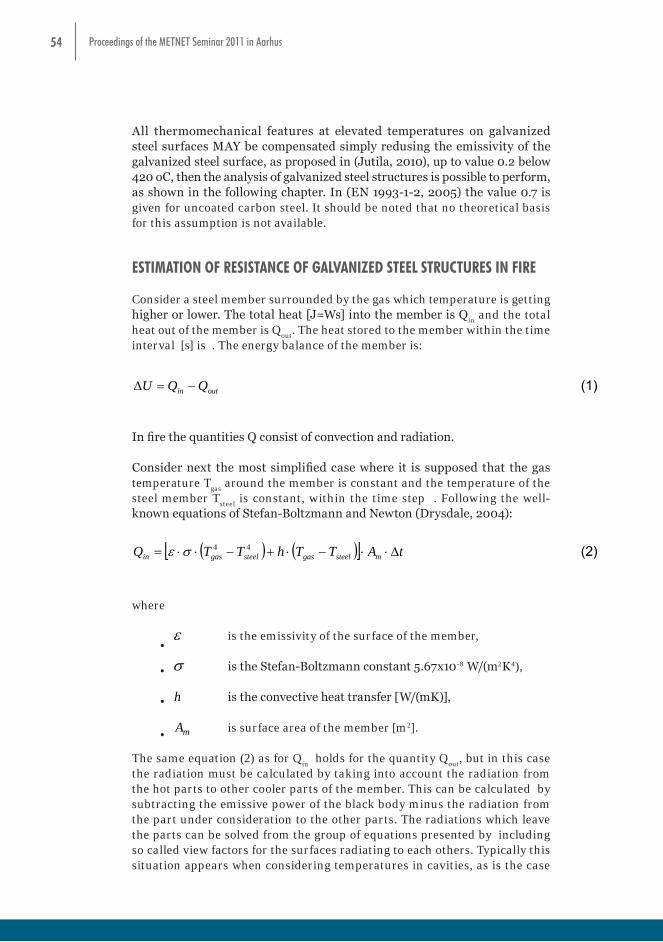
54 Proceedings of the METNET Seminar 2011 in Aarhus
All thermomechanical features at elevated temperatures on galvanized steel surfaces MAY be compensated simply redusing the emissivity of the galvanized steel surface, as proposed in (Jutila, 2010), up to value 0.2 below 420 oC, then the analysis of galvanized steel structures is possible to perform, as shown in the following chapter. In (EN 1993-1-2, 2005) the value 0.7 is given for uncoated carbon steel. It should be noted that no theoretical basis for this assumption is not available.
ESTIMATION OF RESISTANCE OF GALVANIZED STEEL STRUCTURES IN FIRE
Consider a steel member surrounded by the gas which temperature is getting higher or lower. The total heat [J=Ws] into the member is Q
in and the total
heat out of the member is Qout
. The heat stored to the member within the time interval [s] is . The energy balance of the member is:
Consider a steel member surrounded by the gas which temperature is getting higher or lower. The total heat [J=Ws] into the member is Qin and the total heat out of the member is Qout. The heat stored to the member within the time interval t [s] is U . The energy balance of the member is: outin QQU (1) In fire the quantities Q consist of convection and radiation. Consider next the most simplified case where it is supposed that the gas temperature Tgas around the member is constant and the temperature of the steel member Tsteel is constant, within the time step t . Following the well-known equations of Stefan-Boltzmann and Newton (Drysdale, 2004): tATThTTQ msteelgassteelgasin 44 (2)
where is the emissivity of the surface of the member, is the Stefan-Boltzmann constant 5.67x10⁻⁸ W/(m2K4), h is the convective heat transfer [W/(mK)], mA is surface area of the member [m2].
The same equation (2) as for inQ holds for the quantity Qout, but in this case the radiation must be calculated by taking into account the radiation from the hot parts to other cooler parts of the member. This can be calculated by subtracting the emissive power of the black body minus the radiation from the part under consideration to the other parts. The radiations which leave the parts can be solved from the group of equations presented by including so called view factors for the surfaces radiating to each others. Typically this situation appears when considering temperatures in cavities, as is the case when calculating steel temperatures for all metal sandwich panels in fire, as shown in (Ylihärsilä, Heinisuo, 2006). We suppose, that all the parts of the member are at the same temperature, so 0outQ in our case. In the Eurocodes the whole quantity inQ in the equation (2) is multiplied by the “shadow factor” shk . Using this factor the radiation and the convection between different parts of the member is taken into account. There is not radiation or convection between different parts of the member, if they are at the same temperature, as assumed in this study and 1shk . Moreover in Eurocodes, the radiation part of the equation (2) includes a view factor including radiation from the other members. This quantity is supposed to be 1 in this study meaning that steel members do not affect each others. The heat stored to the member during the time interval t is (Drysdale, 2004) supposing, that the whole member gets the same temperature at the same time:
In fire the quantities Q consist of convection and radiation.
Consider next the most simplified case where it is supposed that the gas temperature T
gas around the member is constant and the temperature of the
steel member Tsteel
is constant, within the time step . Following the well-known equations of Stefan-Boltzmann and Newton (Drysdale, 2004):
Consider a steel member surrounded by the gas which temperature is getting higher or lower. The total heat [J=Ws] into the member is Qin and the total heat out of the member is Qout. The heat stored to the member within the time interval t [s] is U . The energy balance of the member is: outin QQU (1) In fire the quantities Q consist of convection and radiation. Consider next the most simplified case where it is supposed that the gas temperature Tgas around the member is constant and the temperature of the steel member Tsteel is constant, within the time step t . Following the well-known equations of Stefan-Boltzmann and Newton (Drysdale, 2004): tATThTTQ msteelgassteelgasin 44 (2)
where is the emissivity of the surface of the member, is the Stefan-Boltzmann constant 5.67x10⁻⁸ W/(m2K4), h is the convective heat transfer [W/(mK)], mA is surface area of the member [m2].
The same equation (2) as for inQ holds for the quantity Qout, but in this case the radiation must be calculated by taking into account the radiation from the hot parts to other cooler parts of the member. This can be calculated by subtracting the emissive power of the black body minus the radiation from the part under consideration to the other parts. The radiations which leave the parts can be solved from the group of equations presented by including so called view factors for the surfaces radiating to each others. Typically this situation appears when considering temperatures in cavities, as is the case when calculating steel temperatures for all metal sandwich panels in fire, as shown in (Ylihärsilä, Heinisuo, 2006). We suppose, that all the parts of the member are at the same temperature, so 0outQ in our case. In the Eurocodes the whole quantity inQ in the equation (2) is multiplied by the “shadow factor” shk . Using this factor the radiation and the convection between different parts of the member is taken into account. There is not radiation or convection between different parts of the member, if they are at the same temperature, as assumed in this study and 1shk . Moreover in Eurocodes, the radiation part of the equation (2) includes a view factor including radiation from the other members. This quantity is supposed to be 1 in this study meaning that steel members do not affect each others. The heat stored to the member during the time interval t is (Drysdale, 2004) supposing, that the whole member gets the same temperature at the same time:
where
• ε is the emissivity of the surface of the member,
• s is the Stefan-Boltzmann constant 5.67x10⁻⁸ W/(m2K4),
• h is the convective heat transfer [W/(mK)],
• mA is surface area of the member [m2].
The same equation (2) as for Qin
holds for the quantity Qout
, but in this case the radiation must be calculated by taking into account the radiation from the hot parts to other cooler parts of the member. This can be calculated by subtracting the emissive power of the black body minus the radiation from the part under consideration to the other parts. The radiations which leave the parts can be solved from the group of equations presented by including so called view factors for the surfaces radiating to each others. Typically this situation appears when considering temperatures in cavities, as is the case
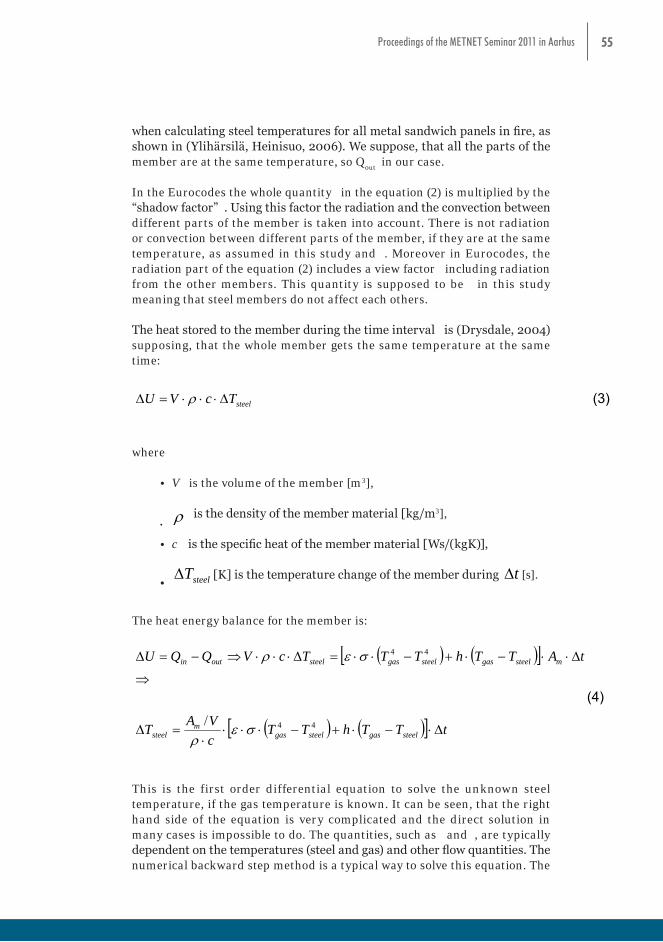
55Proceedings of the METNET Seminar 2011 in Aarhus
All thermomechanical features at elevated temperatures on galvanized steel surfaces MAY be compensated simply redusing the emissivity of the galvanized steel surface, as proposed in (Jutila, 2010), up to value 0.2 below 420 oC, then the analysis of galvanized steel structures is possible to perform, as shown in the following chapter. In (EN 1993-1-2, 2005) the value 0.7 is given for uncoated carbon steel. It should be noted that no theoretical basis for this assumption is not available.
ESTIMATION OF RESISTANCE OF GALVANIZED STEEL STRUCTURES IN FIRE
Consider a steel member surrounded by the gas which temperature is getting higher or lower. The total heat [J=Ws] into the member is Q
in and the total
heat out of the member is Qout
. The heat stored to the member within the time interval [s] is . The energy balance of the member is:
Consider a steel member surrounded by the gas which temperature is getting higher or lower. The total heat [J=Ws] into the member is Qin and the total heat out of the member is Qout. The heat stored to the member within the time interval t [s] is U . The energy balance of the member is: outin QQU (1) In fire the quantities Q consist of convection and radiation. Consider next the most simplified case where it is supposed that the gas temperature Tgas around the member is constant and the temperature of the steel member Tsteel is constant, within the time step t . Following the well-known equations of Stefan-Boltzmann and Newton (Drysdale, 2004): tATThTTQ msteelgassteelgasin 44 (2)
where is the emissivity of the surface of the member, is the Stefan-Boltzmann constant 5.67x10⁻⁸ W/(m2K4), h is the convective heat transfer [W/(mK)], mA is surface area of the member [m2].
The same equation (2) as for inQ holds for the quantity Qout, but in this case the radiation must be calculated by taking into account the radiation from the hot parts to other cooler parts of the member. This can be calculated by subtracting the emissive power of the black body minus the radiation from the part under consideration to the other parts. The radiations which leave the parts can be solved from the group of equations presented by including so called view factors for the surfaces radiating to each others. Typically this situation appears when considering temperatures in cavities, as is the case when calculating steel temperatures for all metal sandwich panels in fire, as shown in (Ylihärsilä, Heinisuo, 2006). We suppose, that all the parts of the member are at the same temperature, so 0outQ in our case. In the Eurocodes the whole quantity inQ in the equation (2) is multiplied by the “shadow factor” shk . Using this factor the radiation and the convection between different parts of the member is taken into account. There is not radiation or convection between different parts of the member, if they are at the same temperature, as assumed in this study and 1shk . Moreover in Eurocodes, the radiation part of the equation (2) includes a view factor including radiation from the other members. This quantity is supposed to be 1 in this study meaning that steel members do not affect each others. The heat stored to the member during the time interval t is (Drysdale, 2004) supposing, that the whole member gets the same temperature at the same time:
In fire the quantities Q consist of convection and radiation.
Consider next the most simplified case where it is supposed that the gas temperature T
gas around the member is constant and the temperature of the
steel member Tsteel
is constant, within the time step . Following the well-known equations of Stefan-Boltzmann and Newton (Drysdale, 2004):
Consider a steel member surrounded by the gas which temperature is getting higher or lower. The total heat [J=Ws] into the member is Qin and the total heat out of the member is Qout. The heat stored to the member within the time interval t [s] is U . The energy balance of the member is: outin QQU (1) In fire the quantities Q consist of convection and radiation. Consider next the most simplified case where it is supposed that the gas temperature Tgas around the member is constant and the temperature of the steel member Tsteel is constant, within the time step t . Following the well-known equations of Stefan-Boltzmann and Newton (Drysdale, 2004): tATThTTQ msteelgassteelgasin 44 (2)
where is the emissivity of the surface of the member, is the Stefan-Boltzmann constant 5.67x10⁻⁸ W/(m2K4), h is the convective heat transfer [W/(mK)], mA is surface area of the member [m2].
The same equation (2) as for inQ holds for the quantity Qout, but in this case the radiation must be calculated by taking into account the radiation from the hot parts to other cooler parts of the member. This can be calculated by subtracting the emissive power of the black body minus the radiation from the part under consideration to the other parts. The radiations which leave the parts can be solved from the group of equations presented by including so called view factors for the surfaces radiating to each others. Typically this situation appears when considering temperatures in cavities, as is the case when calculating steel temperatures for all metal sandwich panels in fire, as shown in (Ylihärsilä, Heinisuo, 2006). We suppose, that all the parts of the member are at the same temperature, so 0outQ in our case. In the Eurocodes the whole quantity inQ in the equation (2) is multiplied by the “shadow factor” shk . Using this factor the radiation and the convection between different parts of the member is taken into account. There is not radiation or convection between different parts of the member, if they are at the same temperature, as assumed in this study and 1shk . Moreover in Eurocodes, the radiation part of the equation (2) includes a view factor including radiation from the other members. This quantity is supposed to be 1 in this study meaning that steel members do not affect each others. The heat stored to the member during the time interval t is (Drysdale, 2004) supposing, that the whole member gets the same temperature at the same time:
where
• is the emissivity of the surface of the member,
• is the Stefan-Boltzmann constant 5.67x10⁻⁸ W/(m2K4),
• is the convective heat transfer [W/(mK)],
• is surface area of the member [m2].
The same equation (2) as for Qin
holds for the quantity Qout
, but in this case the radiation must be calculated by taking into account the radiation from the hot parts to other cooler parts of the member. This can be calculated by subtracting the emissive power of the black body minus the radiation from the part under consideration to the other parts. The radiations which leave the parts can be solved from the group of equations presented by including so called view factors for the surfaces radiating to each others. Typically this situation appears when considering temperatures in cavities, as is the case
when calculating steel temperatures for all metal sandwich panels in fire, as shown in (Ylihärsilä, Heinisuo, 2006). We suppose, that all the parts of the member are at the same temperature, so Q
out in our case.
In the Eurocodes the whole quantity in the equation (2) is multiplied by the “shadow factor” . Using this factor the radiation and the convection between different parts of the member is taken into account. There is not radiation or convection between different parts of the member, if they are at the same temperature, as assumed in this study and . Moreover in Eurocodes, the radiation part of the equation (2) includes a view factor including radiation from the other members. This quantity is supposed to be in this study meaning that steel members do not affect each others.
The heat stored to the member during the time interval is (Drysdale, 2004) supposing, that the whole member gets the same temperature at the same time:
steelTcVU (3) where
V is the volume of the member [m3], is the density of the member material [kg/m3], c is the specific heat of the member material [Ws/(kgK)], steelT [K] is the temperature change of the member during t [s].
The heat energy balance for the member is:
tTThTTcVAT
tATThTTTcVQQU
steelgassteelgasm
steel
msteelgassteelgassteeloutin
44
44
/
(4)
This is the first order differential equation to solve the unknown steel temperature, if the gas temperature is known. It can be seen, that the right hand side of the equation is very complicated and the direct solution in many cases is impossible to do. The quantities, such as c and h , are typically dependent on the temperatures (steel and gas) and other flow quantities. The numerical backward step method is a typical way to solve this equation. The backward method is proper, because the steel temperature is known at the beginning of the time period, at the start of the fire. In the Eurocodes are given the following rule: The time step should not be larger than 5 seconds when solving the equation (4). In many cases this is shown to be very conservative value and larger time steps can be used safely in many cases. Figure 6-7 show steel temperatures for two Am/V values in standard ISO 834 fire. The steel temperatures are calculated using Eq. (4). These are calculated using the constant convection h = 25 W/(m2K). The points proposing Tcr = 500 oC, for design by critical temperatures, are shown in the figures. The results are calculated using (EN 1993-1-2, 2005) and the emissivity value of 0.7 for carbon steel. The emissivity for galvanized steel is assumed to be 0.2 if the steel temperature is below 420oC and 0.7 in the case of steel temperatures higher than 420oC.
where
• V is the volume of the member [m3],
• ρ
is the density of the member material [kg/m3],
• c is the specific heat of the member material [Ws/(kgK)],
• steelT∆ [K] is the temperature change of the member during t∆ [s].
The heat energy balance for the member is:
steelTcVU (3) where
V is the volume of the member [m3], is the density of the member material [kg/m3], c is the specific heat of the member material [Ws/(kgK)], steelT [K] is the temperature change of the member during t [s].
The heat energy balance for the member is:
tTThTTcVAT
tATThTTTcVQQU
steelgassteelgasm
steel
msteelgassteelgassteeloutin
44
44
/
(4)
This is the first order differential equation to solve the unknown steel temperature, if the gas temperature is known. It can be seen, that the right hand side of the equation is very complicated and the direct solution in many cases is impossible to do. The quantities, such as c and h , are typically dependent on the temperatures (steel and gas) and other flow quantities. The numerical backward step method is a typical way to solve this equation. The backward method is proper, because the steel temperature is known at the beginning of the time period, at the start of the fire. In the Eurocodes are given the following rule: The time step should not be larger than 5 seconds when solving the equation (4). In many cases this is shown to be very conservative value and larger time steps can be used safely in many cases. Figure 6-7 show steel temperatures for two Am/V values in standard ISO 834 fire. The steel temperatures are calculated using Eq. (4). These are calculated using the constant convection h = 25 W/(m2K). The points proposing Tcr = 500 oC, for design by critical temperatures, are shown in the figures. The results are calculated using (EN 1993-1-2, 2005) and the emissivity value of 0.7 for carbon steel. The emissivity for galvanized steel is assumed to be 0.2 if the steel temperature is below 420oC and 0.7 in the case of steel temperatures higher than 420oC.
This is the first order differential equation to solve the unknown steel temperature, if the gas temperature is known. It can be seen, that the right hand side of the equation is very complicated and the direct solution in many cases is impossible to do. The quantities, such as and , are typically dependent on the temperatures (steel and gas) and other flow quantities. The numerical backward step method is a typical way to solve this equation. The

56 Proceedings of the METNET Seminar 2011 in Aarhus
backward method is proper, because the steel temperature is known at the beginning of the time period, at the start of the fire. In the Eurocodes are given the following rule: The time step should not be larger than 5 seconds when solving the equation (4). In many cases this is shown to be very conservative value and larger time steps can be used safely in many cases.
Figure 6-7 show steel temperatures for two Am/V values in standard ISO 834 fire. The steel temperatures are calculated using Eq. (4). These are calculated using the constant convection h = 25 W/(m2K). The points proposing Tcr = 500 oC, for design by critical temperatures, are shown in the figures. The results are calculated using (EN 1993-1-2, 2005) and the emissivity value of 0.7 for carbon steel. The emissivity for galvanized steel is assumed to be 0.2 if the steel temperature is below 420oC and 0.7 in the case of steel temperatures higher than 420oC.
Figure 6. Calculated values Am/V=100, standard fire ISO 834
Figure 7. Calculated values Am/V=200, standard fire ISO 834
In the figures can be seen clear time lag in critical temperatures. Critical temperature means in this context temperature when the resistance of the structure is lost, approximatively. Conclusions Clear time lag has been observed in two independent researches between galvanized and uncoated steel members at elevated temperatures. The first minutes in fire are the most critical when considering the actions of fire fighters work, and especially human lives. This
Figure 6. Calculated values Am/V=100, standard fire ISO 834
Figure 6. Calculated values Am/V=100, standard fire ISO 834
Figure 7. Calculated values Am/V=200, standard fire ISO 834
In the figures can be seen clear time lag in critical temperatures. Critical temperature means in this context temperature when the resistance of the structure is lost, approximatively. Conclusions Clear time lag has been observed in two independent researches between galvanized and uncoated steel members at elevated temperatures. The first minutes in fire are the most critical when considering the actions of fire fighters work, and especially human lives. This
Figure 7. Calculated values Am/V=200, standard fire ISO 834

57Proceedings of the METNET Seminar 2011 in Aarhus
In the figures can be seen clear time lag in critical temperatures. Critical temperature means in this context temperature when the resistance of the structure is lost, approximatively.
Conclusions
Clear time lag has been observed in two independent researches between galvanized and uncoated steel members at elevated temperatures. The first minutes in fire are the most critical when considering the actions of fire fighters work, and especially human lives. This means that galvanized steel structures can resist fire better than uncoated steel structures. Thermo-mechanical basis for this observation is still open, but the plan is to work with that in the future. Also aging of galvanizing, effect of different alloys etc are open. However, the effect of galvanizing may mean that in some natural fires no fire protection or slight over-design is enough to reach the required resistance in fire. This means potential to large economical and environmental savings for steel structures.
References
Drysdale, D. An Introduction to Fire Dynamics, Second Editon, Chichester 1998, John Wiley & Sons Ltd. 451 p.
EN 1993-1.2:2005 Eurocode 3: Design of steel structures. Part 1-2: Structural fire design.
Heinisuo, M., Ylihärsilä, H., All metal structures at elevated temperatures. TUT 2006. 54 p. 37 + app.
Jirku J., Transfer of heat to hot dip galvanized elements. Application of Structural Fire Design Conference, Prague, Czech Republic, April 2011.
Jutila H. 2010, Sinkkikerroksen vaikutus teräslevyn emissiviteettiin tulipalossa. Diplomityö s. 86 s. + liitteessä. 18.
58 Proceedings of the METNET Seminar 2011 in Aarhus
EXPERIMENTS OF END PLATE JOINTS IN AMBIENT AND FIRE CONDITIONS UNDER BIAXIAL BENDING
Hilkka Ronni
Henri Perttola
Markku Heinisuo
Tampere University of Technology
Research Centre of Metal Structures
Abstract
Four biaxial bending tests on bolted end plate joints for tubular members with cold formed rectangular hollow steel sections are described. Two pairs of similar joints were tested both in room temperature (ambient conditions) and in fire conditions. The observed failure modes are reported. The described tests belong to the larger series of tests through which the applicability of the component method presented in standard EN1993-1-8 (2005) for the three-dimensional (3D) analysis is investigated. The estimates for the moment resistances in ambient and in elevated temperatures achieved by simplified calculations with the enlarged component method are compared with the test results (four discrete points). Besides this ongoing research of steel joints, the corresponding project for aluminium joints is in progress by our research team in Resarch Center of Metal Structures in Seinäjoki, Finland.
Experimental research
No joint tests on the bolted end plate joints of steel (rectangular or square) tube structures in biaxial bending were found in literature. According to its definition, biaxial bending occurs in the inclined direction. Strictly specifying, in-plane bending and out-of plane bending with resultant moment around the strong axis and, respectively, around the weak axis are then excluded. Murude Celikag and Patrick Kirby have reported on the results of out-of-plane tests (Celikag et al, 1989) for common joint types including flush end plate joints. In their tests, the members connected in joints were British Universal Beams (UB) and Columns (UC), i.e. I- or H-profiles and these tests were arranged as weak axis bending tests. Then (in the late 1980s) Celikag and Kirby suggested that “two similar specimens should be loaded up to the failure in different directions to find out the load carrying capacity of a joint in each direction”. To date, however, most of the joint tests have been arranged in order to study the strong axis bending (in-plane behaviour) of joints and little experimental knowledge is available on the three-dimensional behaviour of the joints. Some information about the out-of-plane bending of bolted steel joints can be found in articles concerned with the joints under earthquake loads (typically
59Proceedings of the METNET Seminar 2011 in Aarhus
horizontal loads in any direction). For example, Lee et al have experimentally investigated the weak axis bending of column bases (Lee et al, 2008).
Even less experimental information exists on the behaviour of the bolted end plate joints of steel (rectangular or square) tubes in biaxial bending under fire conditions than in room temperature. In general, the behaviour of steel and composite joints under fire loading is a subject that has only recently got attention by researchers. A summary of available tests results on steel joints under fire loading can be found in article (Simoes da Silva et al, 2005).
Four biaxial bending tests described in this paper enter into ongoing research about the design method for bolted steel joints and they are reported in detail in yet unpublished tests reports (Ronni and Heinisuo, 2011) and (Perttola and Heinisuo, 2011). A test series “bending tests of bolted end plate joints in cold formed rectangular hollow sections” (Wheeler et al, 1997) including strong axis bending tests only can be regarded as forerunners to the tests series on the tube splices arranged earlier by the authors (Ronni and Heinisuo, 2010). In both of the last named test series one of the main scopes was in the influence of the bolts located outside the edge lines of the cross section in the end plane (called next corner bolts) on the behaviour of the end plate joint. In the four tests described here only the corner bolts were used.
The moment rotation behaviour (stiffness and resistance) of the end plate joints were obtained by the tests in room temperature. Transient type fire tests conducted provided insufficient data for the construction of the moment rotation curve because only one load level was maintained for the considered joint. Instead, the value of critical temperature could be determined by a single test. The main structural parameter varying in the described tests (in ambient or in fire conditions) was the thickness of the end plate (plates with 10 mm and 20 mm nominal thickness were used). Because of the very limited number of the tests considered, only indicative conclusions on the influence of the plate thickness on the joint behaviour could be done.
Component method
The component method, as it is introduced in European Standard EN1993-1-8, is only the starting point to the analysis of the joints described in this paper. Firstly, the inclined direction of the bending associated with the out-of-plane moment rotation response of a joint and, secondly, the lack of the proper equivalent T-stub needed with the corner bolts are outside the application area of the standard. The enlargement because of the out-of-plane bending is done by replacing a joint with the three dimensional (3D) mechanical model called the rake model (Heinisuo et al, 2009). In a rake model, the individual components of a joint are connected through the rigid links (or the rigid plane) to the structural members. The model like this can, in principle, be integrated directly to the (nonlinear) 3D frame analysis or it can be used to study the local response of a joint. The rake model is built up in such a way that the solution in the case of in-plane moment rotation response coincides
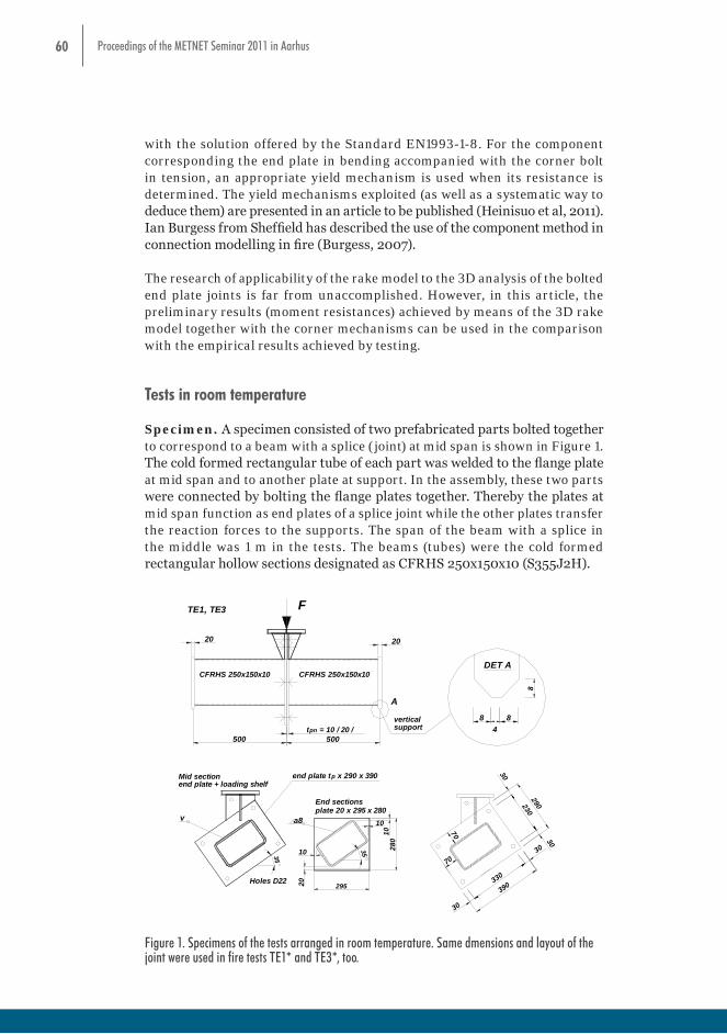
60 Proceedings of the METNET Seminar 2011 in Aarhus
with the solution offered by the Standard EN1993-1-8. For the component corresponding the end plate in bending accompanied with the corner bolt in tension, an appropriate yield mechanism is used when its resistance is determined. The yield mechanisms exploited (as well as a systematic way to deduce them) are presented in an article to be published (Heinisuo et al, 2011). Ian Burgess from Sheffield has described the use of the component method in connection modelling in fire (Burgess, 2007).
The research of applicability of the rake model to the 3D analysis of the bolted end plate joints is far from unaccomplished. However, in this article, the preliminary results (moment resistances) achieved by means of the 3D rake model together with the corner mechanisms can be used in the comparison with the empirical results achieved by testing.
Tests in room temperature
Specimen. A specimen consisted of two prefabricated parts bolted together to correspond to a beam with a splice (joint) at mid span is shown in Figure 1. The cold formed rectangular tube of each part was welded to the flange plate at mid span and to another plate at support. In the assembly, these two parts were connected by bolting the flange plates together. Thereby the plates at mid span function as end plates of a splice joint while the other plates transfer the reaction forces to the supports. The span of the beam with a splice in the middle was 1 m in the tests. The beams (tubes) were the cold formed rectangular hollow sections designated as CFRHS 250x150x10 (S355J2H).
resistances) achieved by means of the 3D rake model together with the corner mechanisms can be used in the comparison with the empirical results achieved by testing. Tests in room temperature Specimen. A specimen consisted of two prefabricated parts bolted together to correspond to a beam with a splice (joint) at mid span is shown in Figure 1. The cold formed rectangular tube of each part was welded to the flange plate at mid span and to another plate at support. In the assembly, these two parts were connected by bolting the flange plates together. Thereby the plates at mid span function as end plates of a splice joint while the other plates transfer the reaction forces to the supports. The span of the beam with a splice in the middle was 1 m in the tests. The beams (tubes) were the cold formed rectangular hollow sections designated as CFRHS 250x150x10 (S355J2H).
500
20
500
CFRHS 250x150x10
20
tpn = 10 / 20 /verticalsupport
35
plate 20 x 295 x 280
Holes D22
v
Mid section
35
CFRHS 250x150x10
TE1, TE3
End sections
end plate tp x 290 x 390
295
a8
F
end plate + loading shelf
280
10
20
10
10
30
230
30
30
30
330
70
70
390
290
8 8
8
4
DET A
A
Figure 1. Specimens of the tests arranged in room temperature. Same dmensions and layout of the joint
were used in fire tests TE1* and TE3*, too. The width and height of the end plates of the splice joints were b = 290 mm and h = 390 mm, respectively. The nominal thicknesses of the end plates were 10 mm, 15 mm and 20 mm. The measured thicknesses of the end plates as well as the material properties of the plates given in the material certificate (based on the tests arranged by the manufacturer) for the corresponding delivery lot are shown in Table 1. It is noteworthy, that the actual thickness of the nominally 10 mm plate was 11.0 mm on average. The placing of the bolt holes in the end plates appears from Figure 1.
Table 1. Thicknesses and material properties of end plates 290x390xtp.
Figure 1. Specimens of the tests arranged in room temperature. Same dmensions and layout of the joint were used in fire tests TE1* and TE3*, too.
61Proceedings of the METNET Seminar 2011 in Aarhus
The width and height of the end plates of the splice joints were b = 290 mm and h = 390 mm, respectively. The nominal thicknesses of the end plates were 10 mm, 15 mm and 20 mm. The measured thicknesses of the end plates as well as the material properties of the plates given in the material certificate (based on the tests arranged by the manufacturer) for the corresponding delivery lot are shown in Table 1. It is noteworthy, that the actual thickness of the nominally 10 mm plate was 11.0 mm on average. The placing of the bolt holes in the end plates appears from Figure 1.
Table 1. Thicknesses and material properties of end plates 290x390xtp.
Tests tpn (nominal)
[mm]
tp (measured)
[mm]
ReH
[MN/m2 ]
Rm
[MN/m2]
A5
%
TE1 and TE1* 10 11.0 429 582 24
TE3 and TE3* 20 20.3 380 564 26
The edges of the tube walls were chamfered for the butt welds connecting the tubes to the end plates. Butt welds were used in an effort to make the influence of weld geometry on joint layout minimal as in the case of ideal joint geometry where there is no outreach of the weld at all. Anyway, the leg lengths of a corresponding “imaginable fillet weld” were estimated to be 2 – 4 mm in the direction of the end plate and 8 -12 mm in the direction of the tube wall. At the supports of the specimen, the tubes were welded to 20 mm plates. The width and height of the plate at supports were 295 mm and 280 mm, respectively
Full thread bolts M20x70 grade 10.9 were used in the joints. The grade of the nuts and the washers (M20) was also 10.9. Three randomly selected bolts were pulled to failure. These tensile tests gave 277.7 kN as the average ultimate load of the bolts. A corresponding tensile strength of 1133 MN/m2 was obtained when a stress area of 245 mm2 was used with the M20 bolt. The bolts situated on the tension side of the joint in bending tests TE3 were tightened to 400 Nm while the tightening moment of the bolts on the compression side was only 70 Nm. Indeviation from the test TE3, the tightening moment of all bolts in test TE1 was 70 Nm.
Test arrangements. The specimen was loaded as a simple beam with the load applied directly to the joint (three-point test). The test set-up used in tests TE1 and TE3 in room temperature is shown in Figure 2. The specimen was placed under the hydraulic jack so that the hinge and the ball joint together allow the movement of the specimen in the transverse but not in the longitudinal direction of the specimen. The transverse degree of freedom must be allowed because transverse displacement inevitably occurs in addition to downward deflection in biaxial bending. The three-point tests were preferred instead of four-point tests with which the constant bending moment in the joint area could have been arranged because of the simplicity of the three point tests.
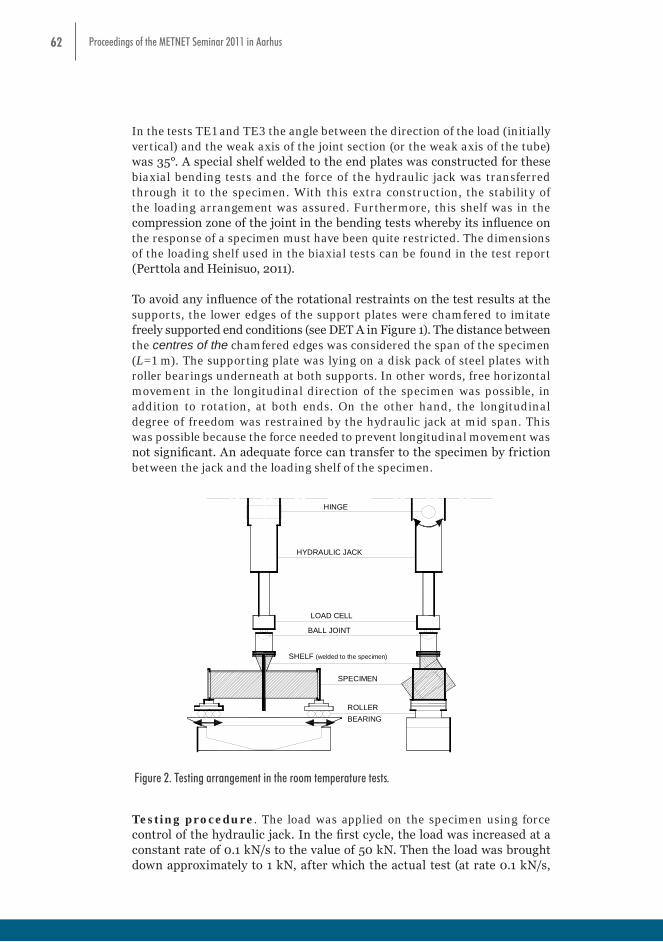
62 Proceedings of the METNET Seminar 2011 in Aarhus
In the tests TE1 and TE3 the angle between the direction of the load (initially vertical) and the weak axis of the joint section (or the weak axis of the tube) was 35°. A special shelf welded to the end plates was constructed for these biaxial bending tests and the force of the hydraulic jack was transferred through it to the specimen. With this extra construction, the stability of the loading arrangement was assured. Furthermore, this shelf was in the compression zone of the joint in the bending tests whereby its influence on the response of a specimen must have been quite restricted. The dimensions of the loading shelf used in the biaxial tests can be found in the test report (Perttola and Heinisuo, 2011).
To avoid any influence of the rotational restraints on the test results at the supports, the lower edges of the support plates were chamfered to imitate freely supported end conditions (see DET A in Figure 1). The distance between the centres of the chamfered edges was considered the span of the specimen (L=1 m). The supporting plate was lying on a disk pack of steel plates with roller bearings underneath at both supports. In other words, free horizontal movement in the longitudinal direction of the specimen was possible, in addition to rotation, at both ends. On the other hand, the longitudinal degree of freedom was restrained by the hydraulic jack at mid span. This was possible because the force needed to prevent longitudinal movement was not significant. An adequate force can transfer to the specimen by friction between the jack and the loading shelf of the specimen.
transfer to the specimen by friction between the jack and the loading shelf of the specimen. Testing procedure. The load was applied on the specimen using force control of the hydraulic jack. In the first cycle, the load was increased at a constant rate of 0.1 kN/s to the value of 50 kN. Then the load was brought down approximately to 1 kN, after which the actual test (at rate 0.1 kN/s, too) up to failure was started. The first cycle was arranged in order to avoid unwanted early stage movements (caused mainly by gaps) in the second cycle. This procedure was followed in the tests TE3 but in the test TE1 the load was removed accidentally almost completely after the first cycle (it was only exception in the test series of twelve tests in all at room temperature).
SPECIMEN
HINGE
BALL JOINT
HYDRAULIC JACK
BEARINGROLLER
SHELF (welded to the specimen)
LOAD CELL
Figure 2. Testing arrangement in the room temperature tests.
Figure 3. Biaxial bending test TE3. Tests in fire Specimen. Similar joints which were tested in room temperature were tested in fire conditions, too. Nominally, the only difference between the specimens in the room
Figure 2. Testing arrangement in the room temperature tests.
Testing procedure. The load was applied on the specimen using force control of the hydraulic jack. In the first cycle, the load was increased at a constant rate of 0.1 kN/s to the value of 50 kN. Then the load was brought down approximately to 1 kN, after which the actual test (at rate 0.1 kN/s,

63Proceedings of the METNET Seminar 2011 in Aarhus
too) up to failure was started. The first cycle was arranged in order to avoid unwanted early stage movements (caused mainly by gaps) in the second cycle. This procedure was followed in the tests TE3 but in the test TE1 the load was removed accidentally almost completely after the first cycle (it was only exception in the test series of twelve tests in all at room temperature).
transfer to the specimen by friction between the jack and the loading shelf of the specimen. Testing procedure. The load was applied on the specimen using force control of the hydraulic jack. In the first cycle, the load was increased at a constant rate of 0.1 kN/s to the value of 50 kN. Then the load was brought down approximately to 1 kN, after which the actual test (at rate 0.1 kN/s, too) up to failure was started. The first cycle was arranged in order to avoid unwanted early stage movements (caused mainly by gaps) in the second cycle. This procedure was followed in the tests TE3 but in the test TE1 the load was removed accidentally almost completely after the first cycle (it was only exception in the test series of twelve tests in all at room temperature).
SPECIMEN
HINGE
BALL JOINT
HYDRAULIC JACK
BEARINGROLLER
SHELF (welded to the specimen)
LOAD CELL
Figure 2. Testing arrangement in the room temperature tests.
Figure 3. Biaxial bending test TE3. Tests in fire Specimen. Similar joints which were tested in room temperature were tested in fire conditions, too. Nominally, the only difference between the specimens in the room
Figure 3. Biaxial bending test TE3.
Tests in fire
Specimen. Similar joints which were tested in room temperature were tested in fire conditions, too. Nominally, the only difference between the specimens in the room temperature tests (TE1, TE3) and in the fire tests (TE1*, TE3*) was the wall thickness of the tube. In tests TE1* and TE3* were used the cold formed rectangular hollow sections CFRHS 250x150x12,5 (S355J2H) instead of profile CFRHS 250x150x10 used in tests TE1 and TE3. However, the difference in tube wall thickness had obviously quite restricted influence or no influence at all on the stiffness and resistance of the joint. This was so because the dimensions of the specimens were selected in such a way that behaviour of the tubes was only in the minor role in all the tests compared with the behaviour of end plates and bolts when stiffness and failure were concerned. The dimensions and layout of the joints in fire tests TE1* and TE3* are shown in Figure 2. The thickness and properties of the end plate are given in Table 1 (plates were taken from the same delivery lot for specimens in room temperature and in fire tests). Similarly, the data concerning bolts, nuts and washers is the same as explained with room temperature tests. The bolts in fire tests were tightened to moment 400 Nm.
Test arrangements/procedure. In the fire tests, the whole specimen was inside the furnace (see schematic representation in Figure 4). The specimens were subjected to ISO834 standard fire which was created by means of 12 gas burners (with the maximum output of 250 kW) in the furnace. The tests were carried out as transient type tests where the loading is constant while the test specimen is heated.

64 Proceedings of the METNET Seminar 2011 in Aarhus
temperature tests (TE1, TE3) and in the fire tests (TE1*, TE3*) was the wall thickness of the tube. In tests TE1* and TE3* were used the cold formed rectangular hollow sections CFRHS 250x150x12,5 (S355J2H) instead of profile CFRHS 250x150x10 used in tests TE1 and TE3. However, the difference in tube wall thickness had obviously quite restricted influence or no influence at all on the stiffness and resistance of the joint. This was so because the dimensions of the specimens were selected in such a way that behaviour of the tubes was only in the minor role in all the tests compared with the behaviour of end plates and bolts when stiffness and failure were concerned. The dimensions and layout of the joints in fire tests TE1* and TE3* are shown in Figure 2. The thickness and properties of the end plate are given in Table 1 (plates were taken from the same delivery lot for specimens in room temperature and in fire tests). Similarly, the data concerning bolts, nuts and washers is the same as explained with room temperature tests. The bolts in fire tests were tightened to moment 400 Nm. Test arrangements/procedure. In the fire tests, the whole specimen was inside the furnace (see schematic representation in Figure 4). The specimens were subjected to ISO834 standard fire which was created by means of 12 gas burners (with the maximum output of 250 kW) in the furnace. The tests were carried out as transient type tests where the loading is constant while the test specimen is heated.
Square hollow sections (SHS):K1, K2, K3 and K4
Chain
Threaded round barThreaded round barTransducer S1 Transducer S2
K2K2
K3
K3
K2
K1
Furnace
Tested specimen
Hydraulic JackHydraulic Jack
K2K2
K2
K1
K3
K4K4
Chain
Tachymeters
Figure 4. Sketch of the testing arrangement in furnace. Measurings by tachymeters were used to verify the
displacements measured by transducers S1 and S2.
The three point (biaxial) bending tests were arranged in such a way that the specimen was supported at mid span and the specimen was pulled at its both ends (Figure 5) through isolated chains by two hydraulic jacks being outside the furnace. Extra plates (t = 20 mm) equipped with the holes were welded to the support plates of the specimen for the hooks of the chains. The span L of the specimen between the suspension points of the specimen was 1040 mm. In the mid span, the similar loading shelf as used with biaxial
Figure 4. Sketch of the testing arrangement in furnace. Measurings by tachymeters were used to verify the displacements measured by transducers S1 and S2.
The three point (biaxial) bending tests were arranged in such a way that the specimen was supported at mid span and the specimen was pulled at its both ends (Figure 5) through isolated chains by two hydraulic jacks being outside the furnace. Extra plates (t = 20 mm) equipped with the holes were welded to the support plates of the specimen for the hooks of the chains. The span L of the specimen between the suspension points of the specimen was 1040 mm. In the mid span, the similar loading shelf as used with biaxial bending tests in room temperature tests took the reaction force. The loading shelf was rigidly connected (welded) to the frame of the furnace.
The chains do not prevent, in principle, any horizontal displacement in the ends of the specimen. Thus, the relative transverse displacement between the mid point and the ends of the specimen was free to occur in the same way as in the room temperature tests. The only axial restraint for the axial movement was at the mid span. Then no compressive force caused by the thermal (axial) expansion of a specimen do not exist. Thus, in fire tests, the joint is under pure bending in the same way as in room temperature tests.
By the control systems of the hydraulic jack, the forces of the jacks were held constant during the fire test. In tests TE1*, the tension force F was 20 kN in both chains and in test TE3* the force F was 30 kN. Thus the sustained bending moments acting on the joint were 10.4 kNm in tests TE1* and 15.6 kNm in tests TE3*, respectively. In the fire test, the heating of the furnace was continued until the specimen (in practice the joint) lost its capacity, i.e. the growth of displacements accelerated rapidly (while the controlling system of the suspension forces was no more able to keep up the load levels).
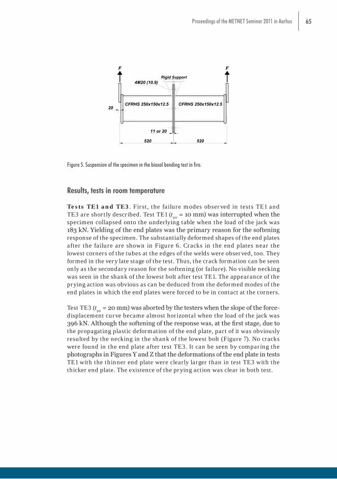
65Proceedings of the METNET Seminar 2011 in Aarhus
bending tests in room temperature tests took the reaction force. The loading shelf was rigidly connected (welded) to the frame of the furnace. The chains do not prevent, in principle, any horizontal displacement in the ends of the specimen. Thus, the relative transverse displacement between the mid point and the ends of the specimen was free to occur in the same way as in the room temperature tests. The only axial restraint for the axial movement was at the mid span. Then no compressive force caused by the thermal (axial) expansion of a specimen do not exist. Thus, in fire tests, the joint is under pure bending in the same way as in room temperature tests. By the control systems of the hydraulic jack, the forces of the jacks were held constant during the fire test. In tests TE1*, the tension force F was 20 kN in both chains and in test TE3* the force F was 30 kN. Thus the sustained bending moments acting on the joint were 10.4 kNm in tests TE1* and 15.6 kNm in tests TE3*, respectively. In the fire test, the heating of the furnace was continued until the specimen (in practice the joint) lost its capacity, i.e. the growth of displacements accelerated rapidly (while the controlling system of the suspension forces was no more able to keep up the load levels).
520
CFRHS 250x150x12.5
4M20 (10.9)
CFRHS 250x150x12.5
11 or 20
20
FF
Rigid Support
520
Figure 5. Suspension of the specimen in the biaxal bending test in fire.
Results, tests in room temperature Tests TE1 and TE3. First, the failure modes observed in tests TE1 and TE3 are shortly described. Test TE1 (tpn = 10 mm) was interrupted when the specimen collapsed onto the underlying table when the load of the jack was 183 kN. Yielding of the end plates was the primary reason for the softening response of the specimen. The substantially deformed shapes of the end plates after the failure are shown in Figure 6. Cracks in the end plates near the lowest corners of the tubes at the edges of the welds were observed, too. They formed in the very late stage of the test. Thus, the crack formation can be seen only as the secondary reason for the softening (or failure). No visible necking was seen in the shank of the lowest bolt after test TE1. The appearance of the prying action was obvious as can be deduced from the deformed modes of the end plates in which the end plates were forced to be in contact at the corners. Test TE3 (tpn = 20 mm) was aborted by the testers when the slope of the force- displacement curve became almost horizontal when the load of the jack was 396 kN. Although the softening of the response was, at the first stage, due to the propagating
Figure 5. Suspension of the specimen in the biaxal bending test in fire.
Results, tests in room temperature
Tests TE1 and TE3. First, the failure modes observed in tests TE1 and TE3 are shortly described. Test TE1 (t
pn = 10 mm) was interrupted when the
specimen collapsed onto the underlying table when the load of the jack was 183 kN. Yielding of the end plates was the primary reason for the softening response of the specimen. The substantially deformed shapes of the end plates after the failure are shown in Figure 6. Cracks in the end plates near the lowest corners of the tubes at the edges of the welds were observed, too. They formed in the very late stage of the test. Thus, the crack formation can be seen only as the secondary reason for the softening (or failure). No visible necking was seen in the shank of the lowest bolt after test TE1. The appearance of the prying action was obvious as can be deduced from the deformed modes of the end plates in which the end plates were forced to be in contact at the corners.
Test TE3 (tpn
= 20 mm) was aborted by the testers when the slope of the force- displacement curve became almost horizontal when the load of the jack was 396 kN. Although the softening of the response was, at the first stage, due to the propagating plastic deformation of the end plate, part of it was obviously resulted by the necking in the shank of the lowest bolt (Figure 7). No cracks were found in the end plate after test TE3. It can be seen by comparing the photographs in Figures Y and Z that the deformations of the end plate in tests TE1 with the thinner end plate were clearly larger than in test TE3 with the thicker end plate. The existence of the prying action was clear in both test.
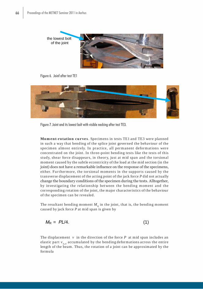
66 Proceedings of the METNET Seminar 2011 in Aarhusplastic deformation of the end plate, part of it was obviously resulted by the necking in the shank of the lowest bolt (Figure 7). No cracks were found in the end plate after test TE3. It can be seen by comparing the photographs in Figures Y and Z that the deformations of the
end plate in tests TE1 with the thinner end plate were clearly larger than in test TE3 with the thicker end plate. The existence of the prying action was clear in both test.
the lowest bolt of the joint
Figure 6. Joinf after test TE1
Figure 7. Joint and its lowest bolt with visible necking after test TE3.
Moment-rotation curves. Specimens in tests TE1 and TE3 were planned in such a way that bending of the splice joint governed the behaviour of the specimen almost entirely. In
practice, all permanent deformations were concentrated on the joint. In three-point bending tests like the tests of this study, shear force disappears, in theory, just at mid span and the
torsional moment caused by the subtle eccentricity of the load at the mid section (in the joint) does not have a remarkable influence on the response of the specimens, either.
Furthermore, the torsional moments in the supports caused by the transverse displacement of the acting point of the jack force P did not actually change the boundary conditions of the specimen during the tests. Alltogether, by investigating the relationship
between the bending moment and the corresponding rotation of the joint, the major characteristics of the behaviour of the specimen can be revealed.
The resultant bending moment MR in the joint, that is, the bending moment caused by jack force P at mid span is given by
MR = PL/4. (1)
The displacement v in the direction of the force P at mid span includes an elastic part vb,el accumulated by the bending deformations across the entire length of the beam. Thus,
the rotation of a joint can be approximated by the formula
Figure 6. Joinf after test TE1
plastic deformation of the end plate, part of it was obviously resulted by the necking in the shank of the lowest bolt (Figure 7). No cracks were found in the end plate after test TE3. It can be seen by comparing the photographs in Figures Y and Z that the deformations of the
end plate in tests TE1 with the thinner end plate were clearly larger than in test TE3 with the thicker end plate. The existence of the prying action was clear in both test.
the lowest bolt of the joint
Figure 6. Joinf after test TE1
Figure 7. Joint and its lowest bolt with visible necking after test TE3.
Moment-rotation curves. Specimens in tests TE1 and TE3 were planned in such a way that bending of the splice joint governed the behaviour of the specimen almost entirely. In
practice, all permanent deformations were concentrated on the joint. In three-point bending tests like the tests of this study, shear force disappears, in theory, just at mid span and the
torsional moment caused by the subtle eccentricity of the load at the mid section (in the joint) does not have a remarkable influence on the response of the specimens, either.
Furthermore, the torsional moments in the supports caused by the transverse displacement of the acting point of the jack force P did not actually change the boundary conditions of the specimen during the tests. Alltogether, by investigating the relationship
between the bending moment and the corresponding rotation of the joint, the major characteristics of the behaviour of the specimen can be revealed.
The resultant bending moment MR in the joint, that is, the bending moment caused by jack force P at mid span is given by
MR = PL/4. (1)
The displacement v in the direction of the force P at mid span includes an elastic part vb,el accumulated by the bending deformations across the entire length of the beam. Thus,
the rotation of a joint can be approximated by the formula
Figure 7. Joint and its lowest bolt with visible necking after test TE3.
Moment-rotation curves. Specimens in tests TE1 and TE3 were planned in such a way that bending of the splice joint governed the behaviour of the specimen almost entirely. In practice, all permanent deformations were concentrated on the joint. In three-point bending tests like the tests of this study, shear force disappears, in theory, just at mid span and the torsional moment caused by the subtle eccentricity of the load at the mid section (in the joint) does not have a remarkable influence on the response of the specimens, either. Furthermore, the torsional moments in the supports caused by the transverse displacement of the acting point of the jack force P did not actually change the boundary conditions of the specimen during the tests. Alltogether, by investigating the relationship between the bending moment and the corresponding rotation of the joint, the major characteristics of the behaviour of the specimen can be revealed.
The resultant bending moment MR in the joint, that is, the bending moment
caused by jack force P at mid span is given by
plastic deformation of the end plate, part of it was obviously resulted by the necking in the shank of the lowest bolt (Figure 7). No cracks were found in the end plate after test TE3. It can be seen by comparing the photographs in Figures Y and Z that the deformations of the end plate in tests TE1 with the thinner end plate were clearly larger than in test TE3 with the thicker end plate. The existence of the prying action was clear in both test. the lowest bolt of the joint
Figure 6. Joinf after test TE1
Figure 7. Joint and its lowest bolt with visible necking after test TE3.
Moment-rotation curves. Specimens in tests TE1 and TE3 were planned in such a way that bending of the splice joint governed the behaviour of the specimen almost entirely. In practice, all permanent deformations were concentrated on the joint. In three-point bending tests like the tests of this study, shear force disappears, in theory, just at mid span and the torsional moment caused by the subtle eccentricity of the load at the mid section (in the joint) does not have a remarkable influence on the response of the specimens, either. Furthermore, the torsional moments in the supports caused by the transverse displacement of the acting point of the jack force P did not actually change the boundary conditions of the specimen during the tests. Alltogether, by investigating the relationship between the bending moment and the corresponding rotation of the joint, the major characteristics of the behaviour of the specimen can be revealed. The resultant bending moment MR in the joint, that is, the bending moment caused by jack force P at mid span is given by MR = PL/4. (1) The displacement v in the direction of the force P at mid span includes an elastic part vb,el accumulated by the bending deformations across the entire length of the beam. Thus, the rotation of a joint can be approximated by the formula θ = 2(v - vb,el ) /L. (2) In the case of the dimensions of the specimens used in tests TE1 and TE3, the reduction term θeb = 2vb,el /L is quite small in comparison with the value of ”the gross rotation” 2v/L. Formulas (1) and (2) define the conversion needed when moment rotation curves based
The displacement v in the direction of the force P at mid span includes an elastic part v
b,el accumulated by the bending
deformations
across the entire
length of the beam. Thus, the rotation of a joint can be approximated by the formula

67Proceedings of the METNET Seminar 2011 in Aarhus
plastic deformation of the end plate, part of it was obviously resulted by the necking in the shank of the lowest bolt (Figure 7). No cracks were found in the end plate after test TE3. It can be seen by comparing the photographs in Figures Y and Z that the deformations of the end plate in tests TE1 with the thinner end plate were clearly larger than in test TE3 with the thicker end plate. The existence of the prying action was clear in both test. the lowest bolt of the joint
Figure 6. Joinf after test TE1
Figure 7. Joint and its lowest bolt with visible necking after test TE3.
Moment-rotation curves. Specimens in tests TE1 and TE3 were planned in such a way that bending of the splice joint governed the behaviour of the specimen almost entirely. In practice, all permanent deformations were concentrated on the joint. In three-point bending tests like the tests of this study, shear force disappears, in theory, just at mid span and the torsional moment caused by the subtle eccentricity of the load at the mid section (in the joint) does not have a remarkable influence on the response of the specimens, either. Furthermore, the torsional moments in the supports caused by the transverse displacement of the acting point of the jack force P did not actually change the boundary conditions of the specimen during the tests. Alltogether, by investigating the relationship between the bending moment and the corresponding rotation of the joint, the major characteristics of the behaviour of the specimen can be revealed. The resultant bending moment MR in the joint, that is, the bending moment caused by jack force P at mid span is given by MR = PL/4. (1) The displacement v in the direction of the force P at mid span includes an elastic part vb,el accumulated by the bending deformations across the entire length of the beam. Thus, the rotation of a joint can be approximated by the formula θ = 2(v - vb,el ) /L. (2) In the case of the dimensions of the specimens used in tests TE1 and TE3, the reduction term θeb = 2vb,el /L is quite small in comparison with the value of ”the gross rotation” 2v/L. Formulas (1) and (2) define the conversion needed when moment rotation curves based In the case of the dimensions of the specimens used in tests TE1 and TE3, the
reduction term θeb
= 2vb,el
/L is quite small in comparison with the value of ”the gross rotation” 2v/L. Formulas (1) and (2) define the conversion needed when moment rotation curves based on the measured quantities are determined. The rotation θ
is defined here as a half of the total rotation of the splice joint
in a way clarified by Figure 8 b. Thus, the rotation θ represents in an average way the deformation of one end plate and half length of the connector (bolt + washer +nut).
The moment-rotation curves (M-θ curves) of the joints achieved by tests TE1 and TE3 are shown in Figure Y. The moment resistance of the joint with the thicker end plate (TE3, t
pn = 20 mm) was approximately 2.2 times larger than
in the case of thinner end plate (TE1, tpn
= 10 mm). Correspondingly, the (intitial) rotational stiffness of the joint was clearly larger when the joint was equipped with the thicker end plate.
Moment‐rotation
0
20
40
60
80
100
0 20 40 60 80 100 120 140 160
Q [mrad]
M [kN
m]
TE3, t=20mm
TE1, t=10mm
on the measured quantities are determined. The rotation θ is defined here as a half of the total rotation of the splice joint in a way clarified by Figure 8 b. Thus, the rotation θ represents in an average way the deformation of one end plate and half length of the connector (bolt + washer +nut). The moment-rotation curves (M-θ curves) of the joints achieved by tests TE1 and TE3 are shown in Figure Y. The moment resistance of the joint with the thicker end plate (TE3, tpn = 20 mm) was approximately 2.2 times larger than in the case of thinner end plate (TE1, tpn = 10 mm). Correspondingly, the (intitial) rotational stiffness of the joint was clearly larger when the joint was equipped with the thicker end plate.
a) b)
Figure 8. a) Moment rotation curves and b) definition of rotation θ.
The numerical values of resistances (Mmax) of a joint achieved by the tests as well as the resistances (MRd) determined by means of the rake model based on the component method are given in Table 2. The resistance of the tension components (end plate in bending and bolt in tension) is defined in accordance with method 2 (see Table 6.2 of EN1993-1-8). Method 2 is relevant only with failure mode 1 (yielding of the flange). In case of joint TE3, the mode 2 (bolt failure with yielding of the flange) governs and the method 2 is irrelevant. It is noteworthy that the failure modes predicted by EN1993-1-8 are in consistent with the observations made in tests TE1 and TE2 (Figures 6 and 7).
Table 2. Moment resistances of joints. Mmax
[kNm] MRd (or MRd,2)
[kNm] MRd/Mmax
TE1 45.7 33.5 0.73 TE3 99.0 69.3 0.70
The values of the moment resistances calculated by the component method for the biaxial tests are on the safe side when compared with the maximum moments defined by tests TE1 and TE3. It will be later returned to this matter in the article. Results, tests in fire
Figure 8. a) Moment rotation curves and b) definition of rotation θ.
The numerical values of resistances (Mmax
) of a joint achieved by the tests as well as the resistances (M
Rd) determined by means of the rake model based
on the component method are given in Table 2. The resistance of the tension components (end plate in bending and bolt in tension) is defined in accordance with method 2 (see Table 6.2 of EN1993-1-8). Method 2 is relevant only with failure mode 1 (yielding of the flange). In case of joint TE3, the mode 2 (bolt failure with yielding of the flange) governs and the method 2 is irrelevant. It is noteworthy that the failure modes predicted by EN1993-1-8 are in consistent with the observations made in tests TE1 and TE2 (Figures 6 and 7).

68 Proceedings of the METNET Seminar 2011 in Aarhus
Table 2. Moment resistances of joints.
Mmax
[kNm]
MRd (or MRd,2)
[kNm]
MRd/Mmax
TE1 45.7 33.5 0.73
TE3 99.0 69.3 0.70
The values of the moment resistances calculated by the component method for the biaxial tests are on the safe side when compared with the maximum moments defined by tests TE1 and TE3. It will be later returned to this matter in the article.
Results, tests in fire
In fire tests TE1* and TE3* the average temperature of the furnace followed to the curve of ISO834 standard fire as shown in Figure 9 in the case of test TE3*. The temperature of the joint was measured on the surface of the end plate in 10 points (see Figure 11 on the right). The temperatures of the bolts were measured during the fire tests, too. The temperature of the joint rose clearly slower than the temperature of the furnace.
0
100
200
300
400
500
600
700
800
900
0 5 10 15 20 25 30 35 40
Tem
pera
ture
[C
]
Time [min]
Furnace
ISO834
Thermocouple average 1-4, in the middle of the side
Thermocouple average 5-10, in the corners
Thermocouple average 11-14, in the bolts
A/V=50
A/V=100
In fire tests TE1* and TE3* the average temperature of the furnace followed to the curve of ISO834 standard fire as shown in Figure 9 in the case of test TE3*. The temperature of the joint was measured on the surface of the end plate in 10 points (see Figure 11 on the right). The temperatures of the bolts were measured during the fire tests, too. The temperature of the joint rose clearly slower than the temperature of the furnace.
Figure
9.
Temperatures in test TE3*.
The values of the resultant bending moments sustained during tests TE1* and TE3* were, respectively, 23% and 16% of those measured as maximum moments in the corresponding room temperature tests (Mmax values are given in Table 2 for room temperature tests TE1 and TE3). It took about 26 min and 28 min in tests TE1* and TE3*, respectively, before the rapid growth of the deformation (in the joints) associated with failure occurred. In Figure 10, the relative vertical displacement of the mid span compared with the average level of the tube ends is presented as a function of temperature T of a joint during the fire tests TE3*. Based on this curve the critical temperature Tcritical was 655 °C. In test TE1*, the critical temperature, in turn, was approximately 800 °C. Failure modes. In test TE1* (tn = 10 mm), failure was due to the large deformations of the end plates (Figure 11, photograph on the left). However, the lowest bolt was stretched clearly more at the high temperature test than in the room temperature test. In spite of this, the appearance of the prying action was obvious as can be seen in the deformed mode of the end plates after the test. Thus, the failure mode observed in test TE1* was quite similar to one at room temperature (see Figure 6). In test TE3* with the thicker end plate tn = 20 mm, the permanent deformations of the end plates were quite moderate as shown in the photograph of Figure 10 taken after the test. The failure mode was the “bolt thread failure” where the lowest bolt slid out from its nut. The observations done during the tests showed that the end plates gradually separated from each other and acceleratingly when the break down approached. Thus, the prying action was not at present (at least in failure) in fire test TE3* opposite to the room temperature test TE3. The influence of the elevated temperature on the threads of the
TE3*
Figure 9. Temperatures in test TE3*.
The values of the resultant bending moments sustained during tests TE1* and TE3* were, respectively, 23% and 16% of those measured as maximum moments in the corresponding room temperature tests (M
max values are given
in Table 2 for room temperature tests TE1 and TE3). It took about 26 min and 28 min in tests TE1* and TE3*, respectively, before the rapid growth of the deformation (in the joints) associated with failure occurred.
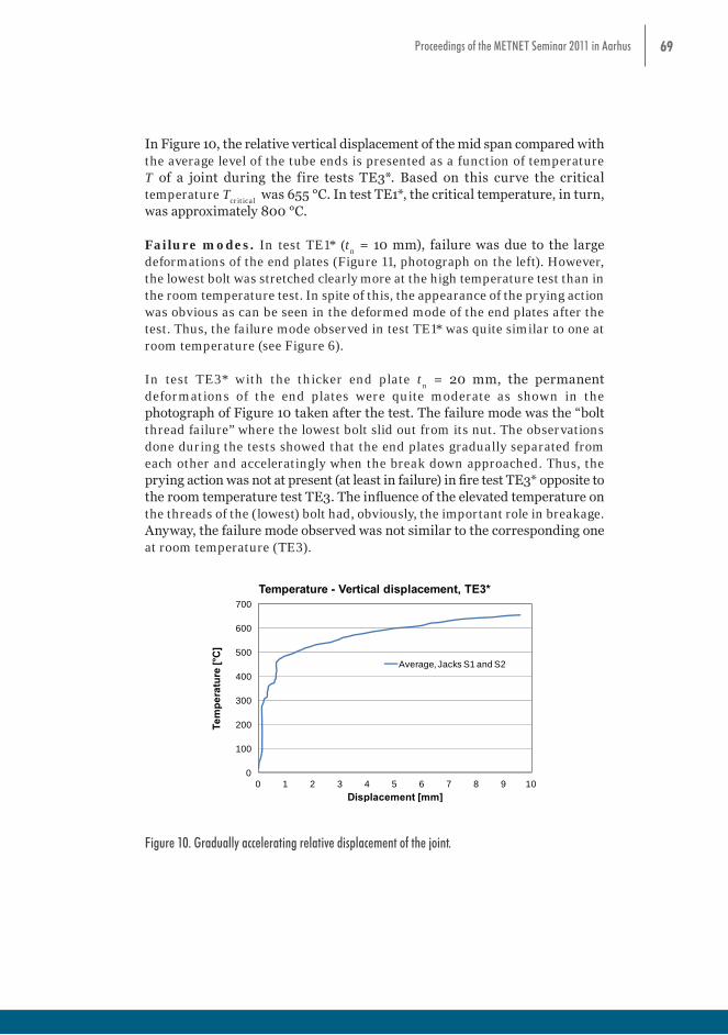
69Proceedings of the METNET Seminar 2011 in Aarhus
In Figure 10, the relative vertical displacement of the mid span compared with the average level of the tube ends is presented as a function of temperature T of a joint during the fire tests TE3*. Based on this curve the critical temperature T
critical was 655 °C. In test TE1*, the critical temperature, in turn,
was approximately 800 °C.
Failure modes. In test TE1* (tn = 10 mm), failure was due to the large
deformations of the end plates (Figure 11, photograph on the left). However, the lowest bolt was stretched clearly more at the high temperature test than in the room temperature test. In spite of this, the appearance of the prying action was obvious as can be seen in the deformed mode of the end plates after the test. Thus, the failure mode observed in test TE1* was quite similar to one at room temperature (see Figure 6).
In test TE3* with the thicker end plate tn = 20 mm, the permanent
deformations of the end plates were quite moderate as shown in the photograph of Figure 10 taken after the test. The failure mode was the “bolt thread failure” where the lowest bolt slid out from its nut. The observations done during the tests showed that the end plates gradually separated from each other and acceleratingly when the break down approached. Thus, the prying action was not at present (at least in failure) in fire test TE3* opposite to the room temperature test TE3. The influence of the elevated temperature on the threads of the (lowest) bolt had, obviously, the important role in breakage. Anyway, the failure mode observed was not similar to the corresponding one at room temperature (TE3).
0
100
200
300
400
500
600
700
0 1 2 3 4 5 6 7 8 9 10
Tem
pera
ture
[°C
]
Displacement [mm]
Temperature - Vertical displacement, TE3*
Average, Jacks S1 and S2
(lowest) bolt had, obviously, the important role in breakage. Anyway, the failure mode observed was not similar to the corresponding one at room temperature (TE3).
Figure 10. Gradually accelerating relative displacement of the joint .
Figure 11. Joints after fire tests. Measuring points of temperature (on right).
Suggestive rake model and test results The moment resistances of the tested joints (TE1, TE3, TE1*, TE3*) were estimated by the three dimensional mechanical model called the rake model. It works like an enlargement of the component method presented in standard EN1993-1-8 and restricted in the strong axis bending of the joint only. The motive to arrange the tests described in this article (and larger series of tests they belong) is in the development of the rake model. The research for this is still going on (2011) and only preliminary results are yet obtained. When the component method is used the properties of individual components had to be determined first. In the most decisive role is the tension component (plate in bending and corner bolt in tension) whose resistance cannot be estimated directly by Standard
1 2
34
11
12
13
14
5 76
8
910
TE3*TE1*
Figure 10. Gradually accelerating relative displacement of the joint.
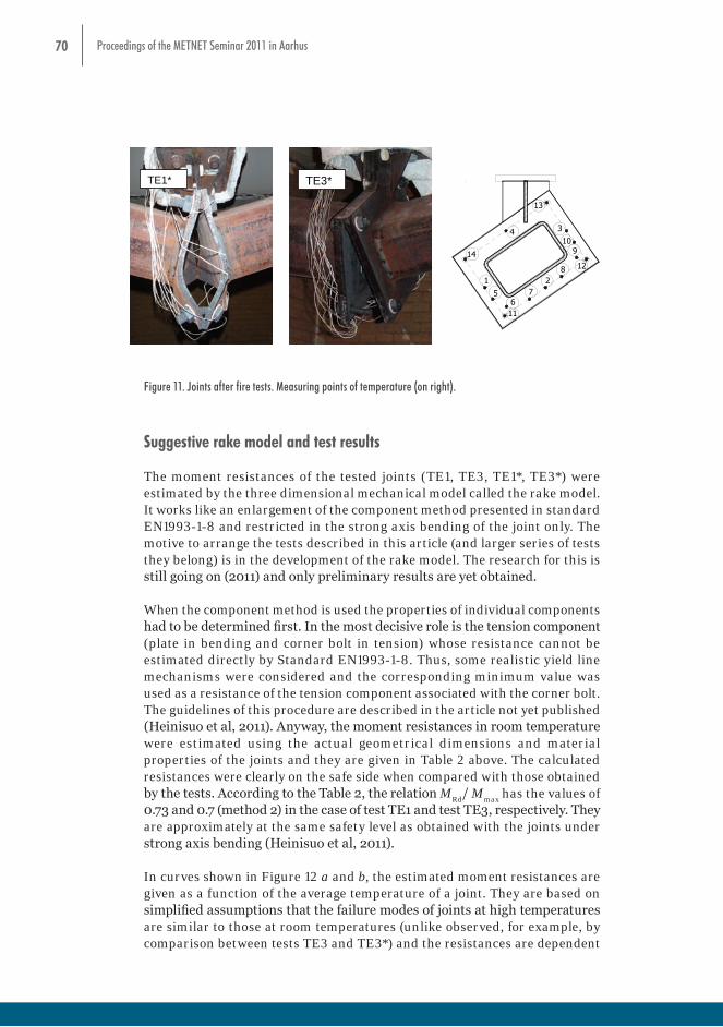
70 Proceedings of the METNET Seminar 2011 in Aarhus
0
100
200
300
400
500
600
700
0 1 2 3 4 5 6 7 8 9 10
Tem
pera
ture
[°C
]
Displacement [mm]
Temperature - Vertical displacement, TE3*
Average, Jacks S1 and S2
(lowest) bolt had, obviously, the important role in breakage. Anyway, the failure mode observed was not similar to the corresponding one at room temperature (TE3).
Figure 10. Gradually accelerating relative displacement of the joint .
Figure 11. Joints after fire tests. Measuring points of temperature (on right).
Suggestive rake model and test results The moment resistances of the tested joints (TE1, TE3, TE1*, TE3*) were estimated by the three dimensional mechanical model called the rake model. It works like an enlargement of the component method presented in standard EN1993-1-8 and restricted in the strong axis bending of the joint only. The motive to arrange the tests described in this article (and larger series of tests they belong) is in the development of the rake model. The research for this is still going on (2011) and only preliminary results are yet obtained. When the component method is used the properties of individual components had to be determined first. In the most decisive role is the tension component (plate in bending and corner bolt in tension) whose resistance cannot be estimated directly by Standard
1 2
34
11
12
13
14
5 76
8
910
TE3*TE1*
Figure 11. Joints after fire tests. Measuring points of temperature (on right).
Suggestive rake model and test results
The moment resistances of the tested joints (TE1, TE3, TE1*, TE3*) were estimated by the three dimensional mechanical model called the rake model. It works like an enlargement of the component method presented in standard EN1993-1-8 and restricted in the strong axis bending of the joint only. The motive to arrange the tests described in this article (and larger series of tests they belong) is in the development of the rake model. The research for this is still going on (2011) and only preliminary results are yet obtained.
When the component method is used the properties of individual components had to be determined first. In the most decisive role is the tension component (plate in bending and corner bolt in tension) whose resistance cannot be estimated directly by Standard EN1993-1-8. Thus, some realistic yield line mechanisms were considered and the corresponding minimum value was used as a resistance of the tension component associated with the corner bolt. The guidelines of this procedure are described in the article not yet published (Heinisuo et al, 2011). Anyway, the moment resistances in room temperature were estimated using the actual geometrical dimensions and material properties of the joints and they are given in Table 2 above. The calculated resistances were clearly on the safe side when compared with those obtained by the tests. According to the Table 2, the relation M
Rd/ M
max has the values of
0.73 and 0.7 (method 2) in the case of test TE1 and test TE3, respectively. They are approximately at the same safety level as obtained with the joints under strong axis bending (Heinisuo et al, 2011).
In curves shown in Figure 12 a and b, the estimated moment resistances are given as a function of the average temperature of a joint. They are based on simplified assumptions that the failure modes of joints at high temperatures are similar to those at room temperatures (unlike observed, for example, by comparison between tests TE3 and TE3*) and the resistances are dependent
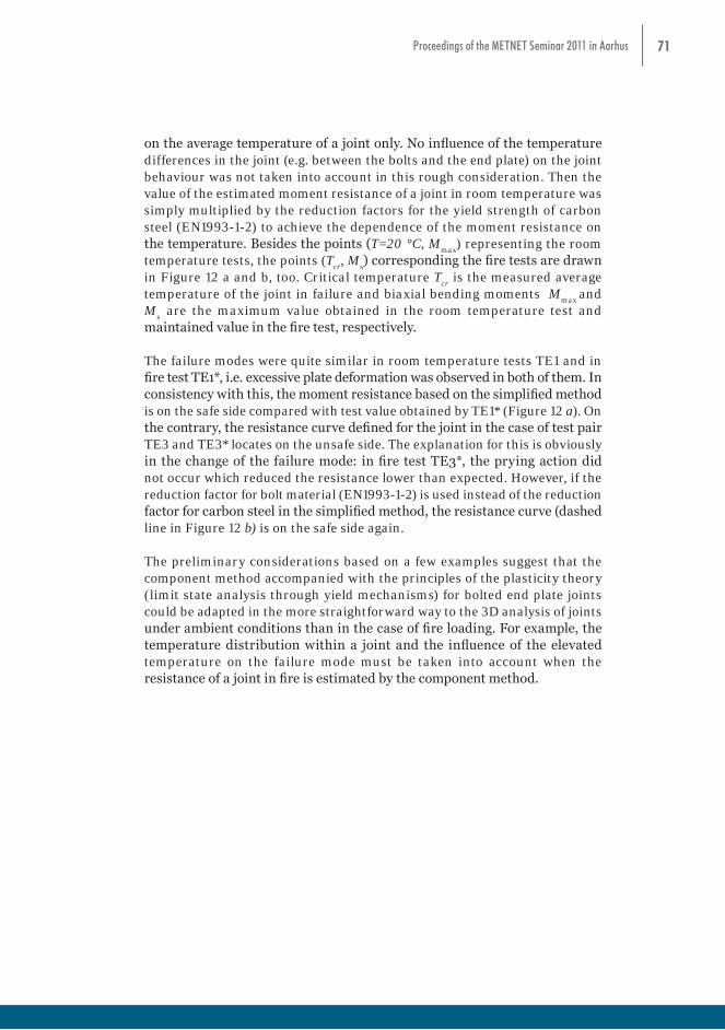
71Proceedings of the METNET Seminar 2011 in Aarhus
on the average temperature of a joint only. No influence of the temperature differences in the joint (e.g. between the bolts and the end plate) on the joint behaviour was not taken into account in this rough consideration. Then the value of the estimated moment resistance of a joint in room temperature was simply multiplied by the reduction factors for the yield strength of carbon steel (EN1993-1-2) to achieve the dependence of the moment resistance on the temperature. Besides the points (T=20 °C, M
max) representing the room
temperature tests, the points (Tcr
, Ms) corresponding the fire tests are drawn
in Figure 12 a and b, too. Critical temperature Tcr
is the measured average temperature of the joint in failure and biaxial bending moments M
max and
Ms
are the maximum value obtained in the room temperature test and maintained value in the fire test, respectively.
The failure modes were quite similar in room temperature tests TE1 and in fire test TE1*, i.e. excessive plate deformation was observed in both of them. In consistency with this, the moment resistance based on the simplified method is on the safe side compared with test value obtained by TE1* (Figure 12 a). On the contrary, the resistance curve defined for the joint in the case of test pair TE3 and TE3* locates on the unsafe side. The explanation for this is obviously in the change of the failure mode: in fire test TE3*, the prying action did not occur which reduced the resistance lower than expected. However, if the reduction factor for bolt material (EN1993-1-2) is used instead of the reduction factor for carbon steel in the simplified method, the resistance curve (dashed line in Figure 12 b) is on the safe side again.
The preliminary considerations based on a few examples suggest that the component method accompanied with the principles of the plasticity theory (limit state analysis through yield mechanisms) for bolted end plate joints could be adapted in the more straightforward way to the 3D analysis of joints under ambient conditions than in the case of fire loading. For example, the temperature distribution within a joint and the influence of the elevated temperature on the failure mode must be taken into account when the resistance of a joint in fire is estimated by the component method.
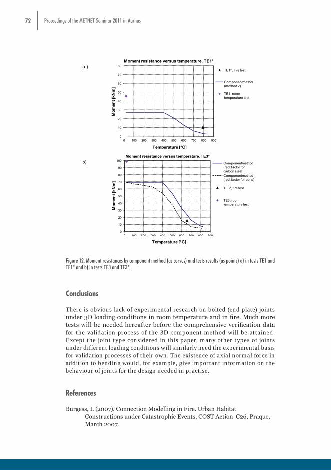
72 Proceedings of the METNET Seminar 2011 in Aarhus
0
10
20
30
40
50
60
70
80
0 100 200 300 400 500 600 700 800 900
Mom
ent [
kNm
]
Temperature [°C]
Moment resistance versus temperature, TE1*
TE1*, fire test
Componentmethod(method 2)
TE1, room temperature test
0
10
20
30
40
50
60
70
80
90
100
0 100 200 300 400 500 600 700 800 900
Mom
ent [
kNm
]
Temperature [°C]
Moment resistance versus temperature, TE3*Componentmethod (red. factor for carbon steel)Componentmethod (red. factor for bolts)
TE3*, fire test
TE3, room temperature test
a )
b)
Figure 12. Moment resistances by component method (as curves) and tests results (as points) a) in tests
TE1 and TE1* and b) in tests TE3 and TE3*. Conclusions There is obvious lack of experimental research on bolted (end plate) joints under 3D loading conditions in room temperature and in fire. Much more tests will be needed hereafter before the comprehensive verification data for the validation process of the 3D component method will be attained. Except the joint type considered in this paper, many other types of joints under different loading conditions will similarly need the experimental basis for validation processes of their own. The existence of axial normal force in addition to bending would, for example, give important information on the behaviour of joints for the design needed in practise.
Figure 12. Moment resistances by component method (as curves) and tests results (as points) a) in tests TE1 and TE1* and b) in tests TE3 and TE3*.
Conclusions
There is obvious lack of experimental research on bolted (end plate) joints under 3D loading conditions in room temperature and in fire. Much more tests will be needed hereafter before the comprehensive verification data for the validation process of the 3D component method will be attained. Except the joint type considered in this paper, many other types of joints under different loading conditions will similarly need the experimental basis for validation processes of their own. The existence of axial normal force in addition to bending would, for example, give important information on the behaviour of joints for the design needed in practise.
References
Burgess, I. (2007). Connection Modelling in Fire. Urban Habitat Constructions under Catastrophic Events, COST Action C26, Praque, March 2007.

73Proceedings of the METNET Seminar 2011 in Aarhus
Celikag, M., Kirby, P. A. (1998). Out-of-plane moment rotation response for common joints. International Colloquium, Bolted and special structural connectors, USSR, Moscow, May 15-20, 1998, pp. 136-142.
EN 1993-1-8 (2005). Eurocode 3: Design of steel structures, Part 1-8: Design of joints, CEN, Brussels.
EN 1993-1-2 (2005). Eurocode 3: Design of steel structures, Part 1-2: General rules – Structural fire design, CEN, Brussels.
Heinisuo, M., Laine, V., Lehtimäki, E. (2009), Enlargement of the component method into 3D, Proceedings: Nordic Steel Constructional Conference 2009, Malmö, Sweden, September 2-4, 2009, pp. 430-437.
Lee, D-Y., Goel, S., Stojadinovich, B. (2008), Exposed Column-Base Plate Connections Bending About Weak Axis: II. Experimental Study, Steel Structures, Vol. 8, 2008, pp. 29-42.
Ronni, H., Heinisuo, M. (2011). Test Report, End Plate Joints of Steel Tubes, Strong Axis Bending, Research Report 149, Tampere University of Technology, Department of Civil Engineering, Structural Engineering, 2010.
Simoes da Silva, L., Vila Real, P., Moore, D., (2005). Behaviour of steel joints under fire loading, Steel and Composite Structures, Vol. 5, No. 6, 2005, pp. 485-513.
Wheeler, A, Clarke, M, Hancock, G, (1997), Bending Tests of Bolted End Plate Connections in Cold Formed Rectangular Hollow Sections”, Research Report No. R736, The University of Sydney, Department of Civil Engineering, Centre of Advanced Structural Engineering, Sydney, 1997.
▪To be published by the research group of RCMT (Research Centre of Metal Structures):
Heinisuo M., Ronni H., Perttola H., Aalto A., Tiainen T. (2011), Bolted end plate joints of rectangular tubular members, in review.
Perttola H., Heinisuo, M. (2011), Test Report, End Plate Joints of Steel Tubes, Biaxial and Weak Axis Bending Tests, Research Report 155, Tampere University of Technology, Department of Civil Engineering, Structural Engineering, 2010.
Ronni, H., Heinisuo, M. (2011), Test Report, End Plate Joints of Steel Tubes, Biaxial Bending Tests in Fire, Research Report 156, Tampere University of Technology, Department of Civil Engineering, Structural Engineering, 2010.
74 Proceedings of the METNET Seminar 2011 in Aarhus
FIRE DESIGN OF A STEEL HALL WITHOUT FIRE PROTECTION
Patrik Takács*
László Horváth*
István Szontagh**
*Department of Structural Engineering
Budapest University of Technology and Economics, Hungary
**Ruukki Hungary Ltd.
Abstract
In Hungary only since 2008 is allowed to use the structural fire engineering methods for fire design. The Eurocode provides methods and standards for these calculations. The practising engineers have no experience to apply these methods; therefore studies are made about them, like this, which is based on a bachelor thesis work. Our intention is also dual. First we study the fire design process of the frequently used steel structures and present it to the practising engineers. On the other hand we analyse the maximum fire resistance of these unprotected steel structures, and looking for different methods to fulfil the requirements of R30 fire resistance class.
The structure
The designed building is a standard Ruukki industrial steel hall shown in Figure 1 with a storage function. It has an area of 30×50m. The primary load-bearing structural elements are portal frames from hollow-sectioned trusses and steel columns with non-uniform welded I-sections. The global stability of the structure is provided by the bracing system. The applied steel grade is S355.The building is covered by sandwich panels, which are fixed to the purlins.
Requirements
The requirements of the fire design are written in the National Fire Regulations of Hungary (NFR-OTSZ, 2008). It is depend on the function of the building, the number of storeys, the specific fire load and the area of the analysed fire compartment. The designed steel hall has only one storey. The specific fire load is lower than 250MJ/m2, because only non-combustible materials are stored there, so the building belongs to the „E” fire risk class. The building has only one fire compartment area, which is the whole area, and it is below 1500m2, therefore it belongs to the IV. fire resistance category.
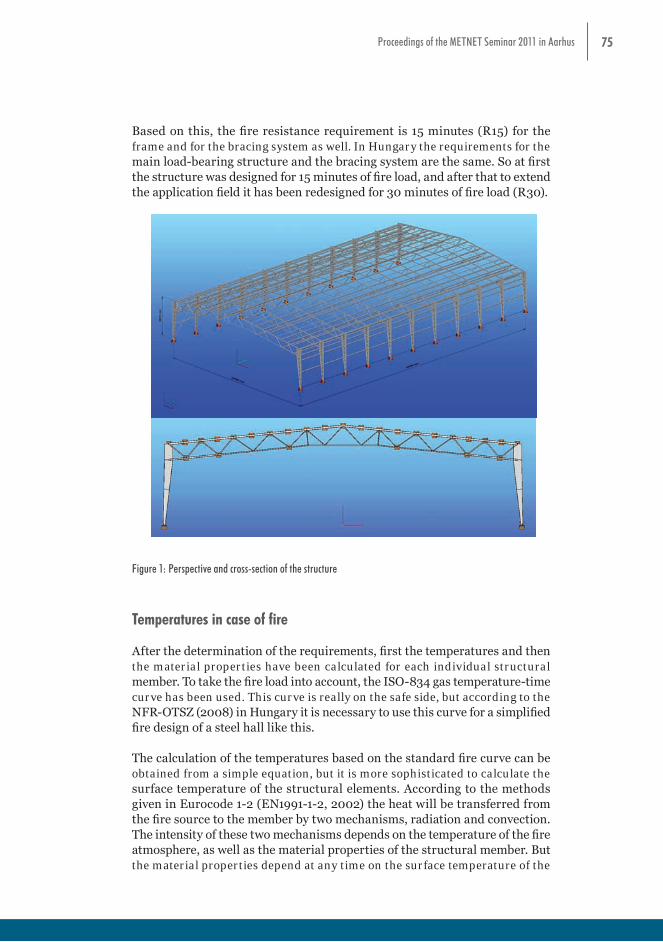
75Proceedings of the METNET Seminar 2011 in Aarhus
Based on this, the fire resistance requirement is 15 minutes (R15) for the frame and for the bracing system as well. In Hungary the requirements for the main load-bearing structure and the bracing system are the same. So at first the structure was designed for 15 minutes of fire load, and after that to extend the application field it has been redesigned for 30 minutes of fire load (R30).
Figure 1: Perspective and cross-section of the structure
Temperatures in case of fire
After the determination of the requirements, first the temperatures and then the material properties have been calculated for each individual structural member. To take the fire load into account, the ISO-834 gas temperature-time curve has been used. This curve is really on the safe side, but according to the NFR-OTSZ (2008) in Hungary it is necessary to use this curve for a simplified fire design of a steel hall like this.
The calculation of the temperatures based on the standard fire curve can be obtained from a simple equation, but it is more sophisticated to calculate the surface temperature of the structural elements. According to the methods given in Eurocode 1-2 (EN1991-1-2, 2002) the heat will be transferred from the fire source to the member by two mechanisms, radiation and convection. The intensity of these two mechanisms depends on the temperature of the fire atmosphere, as well as the material properties of the structural member. But the material properties depend at any time on the surface temperature of the member, therefore member temperature is related to time via a fairly complex differential equation. Eurocode 1-2 (EN1991-1-2, 2002) allows calculating the temperature increments progressively in equal time intervals, which can not be more than 5 seconds. So the temperatures and the material properties have been calculated for each individual structural component in every 5 seconds with Microsoft Excel. These temperature-dependent properties, shown in Figure 2, are the modulus of elasticity, the coefficient of thermal expansion, and the yield strength, which will be also required by the creating of the
Figure 1: Perspective and cross-section of the structure
Temperatures in case of fire
After the determination of the requirements, first the temperatures and then the material properties have been calculated for each individual structural member. To take the fire load into account, the ISO-834 gas temperature-time curve has been used. This curve is really on the safe side, but according to the NFR-OTSZ (2008) in Hungary it is necessary to use this curve for a simplified fire design of a steel hall like this.
The calculation of the temperatures based on the standard fire curve can be obtained from a simple equation, but it is more sophisticated to calculate the surface temperature of the structural elements. According to the methods given in Eurocode 1-2 (EN1991-1-2, 2002) the heat will be transferred from the fire source to the member by two mechanisms, radiation and convection. The intensity of these two mechanisms depends on the temperature of the fire atmosphere, as well as the material properties of the structural member. But the material properties depend at any time on the surface temperature of the
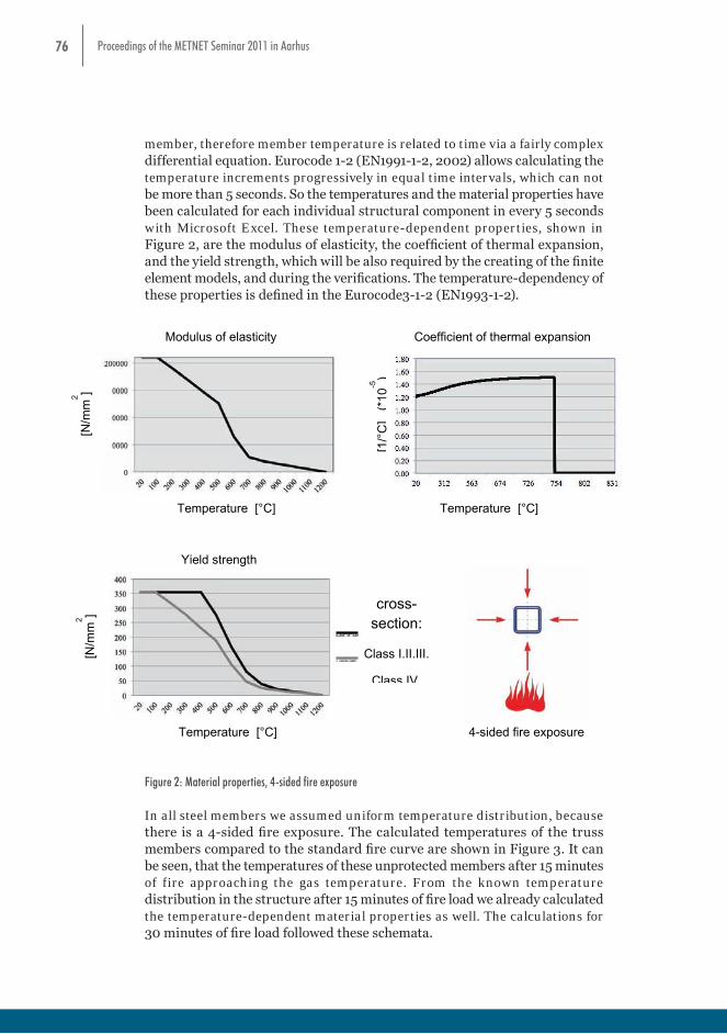
76 Proceedings of the METNET Seminar 2011 in Aarhus
member, therefore member temperature is related to time via a fairly complex differential equation. Eurocode 1-2 (EN1991-1-2, 2002) allows calculating the temperature increments progressively in equal time intervals, which can not be more than 5 seconds. So the temperatures and the material properties have been calculated for each individual structural component in every 5 seconds with Microsoft Excel. These temperature-dependent properties, shown in Figure 2, are the modulus of elasticity, the coefficient of thermal expansion, and the yield strength, which will be also required by the creating of the finite element models, and during the verifications. The temperature-dependency of these properties is defined in the Eurocode3-1-2 (EN1993-1-2).finite element models, and during the verifications. The temperature-dependency of these
properties is defined in the Eurocode3-1-2 (EN1993-1-2).
Figure 2: Material properties, 4-sided fire exposure
In all steel members we assumed uniform temperature distribution, because there is a 4-sided fire exposure. The calculated temperatures of the truss members compared to the standard fire curve are shown in Figure 3. It can be seen, that the temperatures of these unprotected members after 15 minutes of fire approaching the gas temperature. From the known temperature distribution in the structure after 15 minutes of fire load we already calculated the temperature-dependent material properties as well. The calculations for 30 minutes of fire load followed these schemata.
Temperature [°C] Temperature [°C]
[1/°
C]
(*10
-5)
Modulus of elasticity Coefficient of thermal expansion
[N/m
m2 ]
Yield strength
[N/m
m2 ]
Temperature [°C] 4-sided fire exposure
cross-section:
Class I.II.III.
Class IV
Figure 2: Material properties, 4-sided fire exposure
In all steel members we assumed uniform temperature distribution, because there is a 4-sided fire exposure. The calculated temperatures of the truss members compared to the standard fire curve are shown in Figure 3. It can be seen, that the temperatures of these unprotected members after 15 minutes of fire approaching the gas temperature. From the known temperature distribution in the structure after 15 minutes of fire load we already calculated the temperature-dependent material properties as well. The calculations for 30 minutes of fire load followed these schemata.
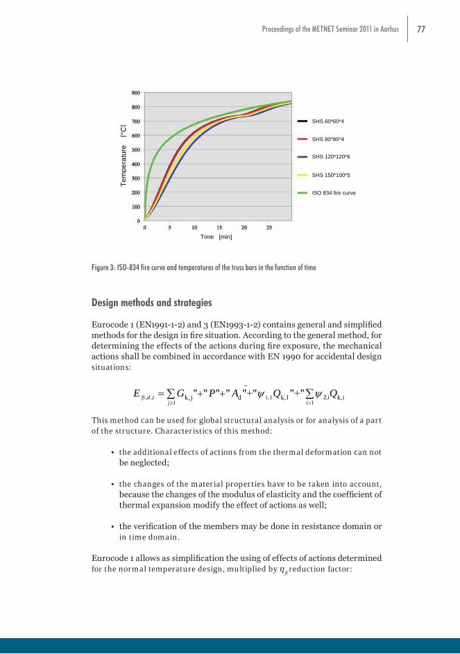
77Proceedings of the METNET Seminar 2011 in Aarhus
Figure 3:
ISO-
834 fire curv
e and temperatures of the trus
s bars in the function of
time Design methods and strategies Eurocode 1 (EN1991-1-2) and 3 (EN1993-1-2) contains general and simplified methods for the design in fire situation. According to the general method, for determining the effects of the actions during fire exposure, the mechanical actions shall be combined in accordance with EN 1990 for accidental design situations:
1i
1,11
,, ik,k,1djk, "+""+""""" QQAPGEj
tdfi i2,
This method can be used for global structural analysis or for analysis of a part of the structure. Characteristics of this method:
the additional effects of actions from the thermal deformation can not be neglected; the changes of the material properties have to be taken into account, because the
changes of the modulus of elasticity and the coefficient of thermal expansion modify the effect of actions as well;
the verification of the members may be done in resistance domain or in time domain.
Eurocode 1 allows as simplification the using of effects of actions determined for the normal temperature design, multiplied by ηfi reduction factor:
dfitdfi EE ..
where ηfi is defined by the following equation:
1.1.
1.1.1
kQkG
kkGAfi QG
QG
Time [min]
Tem
pera
ture
[°
C]
SHS 150*100*5
SHS 120*120*6
SHS 80*80*4
SHS 60*60*4
ISO 834 fire curve
Figure 3: ISO-834 fire curve and temperatures of the truss bars in the function of time
Design methods and strategies
Eurocode 1 (EN1991-1-2) and 3 (EN1993-1-2) contains general and simplified methods for the design in fire situation. According to the general method, for determining the effects of the actions during fire exposure, the mechanical actions shall be combined in accordance with EN 1990 for accidental design situations:
Figure 3:
ISO-
834 fire curv
e and temperatures of the trus
s bars in the function of
time Design methods and strategies Eurocode 1 (EN1991-1-2) and 3 (EN1993-1-2) contains general and simplified methods for the design in fire situation. According to the general method, for determining the effects of the actions during fire exposure, the mechanical actions shall be combined in accordance with EN 1990 for accidental design situations:
1i
1,11
,, ik,k,1djk, "+""+""""" QQAPGEj
tdfi i2,
This method can be used for global structural analysis or for analysis of a part of the structure. Characteristics of this method:
the additional effects of actions from the thermal deformation can not be neglected; the changes of the material properties have to be taken into account, because the
changes of the modulus of elasticity and the coefficient of thermal expansion modify the effect of actions as well;
the verification of the members may be done in resistance domain or in time domain.
Eurocode 1 allows as simplification the using of effects of actions determined for the normal temperature design, multiplied by ηfi reduction factor:
dfitdfi EE ..
where ηfi is defined by the following equation:
1.1.
1.1.1
kQkG
kkGAfi QG
QG
Time [min]
Tem
pera
ture
[°
C]
SHS 150*100*5
SHS 120*120*6
SHS 80*80*4
SHS 60*60*4
ISO 834 fire curve
This method can be used for global structural analysis or for analysis of a part of the structure. Characteristics of this method:
• the additional effects of actions from the thermal deformation can not be neglected;
• the changes of the material properties have to be taken into account, because the changes of the modulus of elasticity and the coefficient of thermal expansion modify the effect of actions as well;
• the verification of the members may be done in resistance domain or in time domain.
Eurocode 1 allows as simplification the using of effects of actions determined for the normal temperature design, multiplied by η
fi reduction factor:
78 Proceedings of the METNET Seminar 2011 in Aarhus
Figure 3:
ISO-
834 fire curv
e and temperatures of the trus
s bars in the function of
time Design methods and strategies Eurocode 1 (EN1991-1-2) and 3 (EN1993-1-2) contains general and simplified methods for the design in fire situation. According to the general method, for determining the effects of the actions during fire exposure, the mechanical actions shall be combined in accordance with EN 1990 for accidental design situations:
1i
1,11
,, ik,k,1djk, "+""+""""" QQAPGEj
tdfi i2,
This method can be used for global structural analysis or for analysis of a part of the structure. Characteristics of this method:
the additional effects of actions from the thermal deformation can not be neglected; the changes of the material properties have to be taken into account, because the
changes of the modulus of elasticity and the coefficient of thermal expansion modify the effect of actions as well;
the verification of the members may be done in resistance domain or in time domain.
Eurocode 1 allows as simplification the using of effects of actions determined for the normal temperature design, multiplied by ηfi reduction factor:
dfitdfi EE ..
where ηfi is defined by the following equation:
1.1.
1.1.1
kQkG
kkGAfi QG
QG
Time [min]
Tem
pera
ture
[°
C]
SHS 150*100*5
SHS 120*120*6
SHS 80*80*4
SHS 60*60*4
ISO 834 fire curve
where ηfi is defined by the following equation:
Figure 3:
ISO-
834 fire curv
e and temperatures of the trus
s bars in the function of
time Design methods and strategies Eurocode 1 (EN1991-1-2) and 3 (EN1993-1-2) contains general and simplified methods for the design in fire situation. According to the general method, for determining the effects of the actions during fire exposure, the mechanical actions shall be combined in accordance with EN 1990 for accidental design situations:
1i
1,11
,, ik,k,1djk, "+""+""""" QQAPGEj
tdfi i2,
This method can be used for global structural analysis or for analysis of a part of the structure. Characteristics of this method:
the additional effects of actions from the thermal deformation can not be neglected; the changes of the material properties have to be taken into account, because the
changes of the modulus of elasticity and the coefficient of thermal expansion modify the effect of actions as well;
the verification of the members may be done in resistance domain or in time domain.
Eurocode 1 allows as simplification the using of effects of actions determined for the normal temperature design, multiplied by ηfi reduction factor:
dfitdfi EE ..
where ηfi is defined by the following equation:
1.1.
1.1.1
kQkG
kkGAfi QG
QG
Time [min]
Tem
pera
ture
[°
C]
SHS 150*100*5
SHS 120*120*6
SHS 80*80*4
SHS 60*60*4
ISO 834 fire curve
Characteristics of this method:
• in Hungary (NFR-OTSZ, 2008) it can only be used with the standard fire curve;
• it can be used only together with the resistance check of all the structural members;
• when both the requirements listed above are fulfilled, then additional effects of actions from the thermal deformation should not be taken into account.
The simplest way is the critical temperature method. It can only be used, when no stability loss may occur. With this method it is not necessary to calculate the member resistance, only the temperature of the member after the fire duration should be determined. The critical temperature of Class I, II, and III cross-sections is based on the degree of utilization, where the critical temperature of the very slender Class IV sections is uniformly 350°C.
In this study we used all above-mentioned methods and compared the results.
Finite element models
According to the general method, in accidental design situation the global structural analysis was performed by the Consteel 6.0 finite element & steel design software. Two types of finite element models have been used, one individual finite element model, and a second model created by the Consteel’s new fire-module. Moreover, these two types of finite element models have been created in 2D and in 3D as well, because the frame was analyzed with a two-dimensional model and the bracing system was analyzed with a three-dimensional model. The models are shown in Figure 4.
Altogether 12 finite element models have been created because of the normal temperature models and the two types of models in case of fire, the 2D and the 3D models, and because of the 15 and the 30 minutes of fire load.
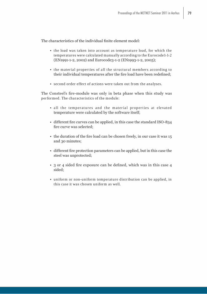
79Proceedings of the METNET Seminar 2011 in Aarhus
The characteristics of the individual finite element model:
• the load was taken into account as temperature load, for which the temperatures were calculated manually according to the Eurocode1-1-2 (EN1991-1-2, 2002) and Eurocode3-1-2 (EN1993-1-2, 2005);
• the material properties of all the structural members according to their individual temperatures after the fire load have been redefined;
• second order effect of actions were taken out from the analyses.
The Consteel’s fire-module was only in beta phase when this study was performed. The characteristics of the module:
• all the temperatures and the material properties at elevated temperature were calculated by the software itself;
• different fire curves can be applied, in this case the standard ISO-834 fire curve was selected;
• the duration of the fire load can be chosen freely, in our case it was 15 and 30 minutes;
• different fire protection parameters can be applied, but in this case the steel was unprotected;
• 3 or 4 sided fire exposure can be defined, which was in this case 4 sided;
• uniform or non-uniform temperature distribution can be applied, in this case it was chosen uniform as well.
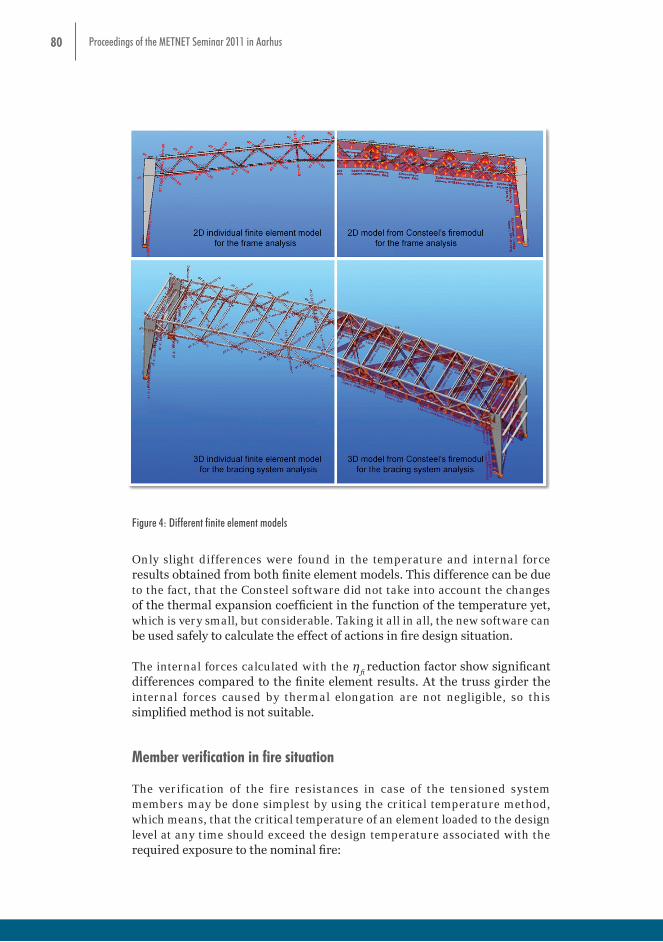
80 Proceedings of the METNET Seminar 2011 in Aarhus
3 or 4 sided fire exposure can be defined, which was in this case 4 sided; uniform or non-uniform temperature distribution can be applied, in this case it was
chosen uniform as well.
Figure 4: Different finite element models
Only slight differences were found in the temperature and internal force results obtained from both finite element models. This difference can be due to the fact, that the Consteel software did not take into account the changes of the thermal expansion coefficient in the function of the temperature yet, which is very small, but considerable. Taking it all in all, the new software can be used safely to calculate the effect of actions in fire design situation. The internal forces calculated with the ηfi reduction factor show significant differences compared to the finite element results. At the truss girder the internal forces caused by thermal elongation are not negligible, so this simplified method is not suitable. Member verification in fire situation The verification of the fire resistances in case of the tensioned system members may be done simplest by using the critical temperature method, which means, that the critical temperature of an element loaded to the design level at any time should exceed the design temperature associated with the required exposure to the nominal fire:
Figure 4: Different finite element models
Only slight differences were found in the temperature and internal force results obtained from both finite element models. This difference can be due to the fact, that the Consteel software did not take into account the changes of the thermal expansion coefficient in the function of the temperature yet, which is very small, but considerable. Taking it all in all, the new software can be used safely to calculate the effect of actions in fire design situation.
The internal forces calculated with the ηfi
reduction factor show significant differences compared to the finite element results. At the truss girder the internal forces caused by thermal elongation are not negligible, so this simplified method is not suitable.
Member verification in fire situation
The verification of the fire resistances in case of the tensioned system members may be done simplest by using the critical temperature method, which means, that the critical temperature of an element loaded to the design level at any time should exceed the design temperature associated with the required exposure to the nominal fire:

81Proceedings of the METNET Seminar 2011 in Aarhus
ddcr , According to the general method, the load-bearing resistance of the members should be checked:
tdfitdfi ER ,,,,
For these calculations the Eurocode3-1-2 (EN1993-1-2, 2005) gives the resistances of the members in fire design situation by similar equations as in normal temperature design, but with reduced strength and deformation properties and with modified partial factor for the relevant material property. Usually the ky,θ is the reduction factor for the yield strength of steel at the maximum temperature of the member, and the stability reduction factors should be determined differently in fire situation. We performed the check of the tensioned truss and tensioned bracing system members with both of these methods and found no mentionable differences. The verification of the other members has been done by calculating their resistances. At normal temperature, the verification and the stability analysis of all members can be easily done with the Consteel software, which is able to perform it with the global stability analysis of the whole structure or sub-structure. In case of fire, because of the lack of the software development, the verification and the stability analysis can only be done on each structural component individually and manually. Special problem was the check of the tapered column. This is not so obvious, because there are not any standardized methods to perform the stability analysis of a tapered column. Therefore first a replacing column member was created (see Figure 5). The cross-sections of the replacing column were taken from the half of the sideway supported parts of the original column. With this method we got 4 different, but uniform column parts. Then the verification could be done on this replacing column manually, stepwise on each column parts. The cross-sections of the column are Class 4 cross-sections; therefore first the effective cross-sections have been calculated. Then the cross-section resistance verifications have been done in case of the tensioned/compressed, sheared and bended column parts as well. For the verification of the stability, first a buckling analysis in both direction and a lateral-torsional buckling analysis were performed, than the combined effects were checked.
According to the general method, the load-bearing resistance of the members should be checked:
ddcr , According to the general method, the load-bearing resistance of the members should be checked:
tdfitdfi ER ,,,,
For these calculations the Eurocode3-1-2 (EN1993-1-2, 2005) gives the resistances of the members in fire design situation by similar equations as in normal temperature design, but with reduced strength and deformation properties and with modified partial factor for the relevant material property. Usually the ky,θ is the reduction factor for the yield strength of steel at the maximum temperature of the member, and the stability reduction factors should be determined differently in fire situation. We performed the check of the tensioned truss and tensioned bracing system members with both of these methods and found no mentionable differences. The verification of the other members has been done by calculating their resistances. At normal temperature, the verification and the stability analysis of all members can be easily done with the Consteel software, which is able to perform it with the global stability analysis of the whole structure or sub-structure. In case of fire, because of the lack of the software development, the verification and the stability analysis can only be done on each structural component individually and manually. Special problem was the check of the tapered column. This is not so obvious, because there are not any standardized methods to perform the stability analysis of a tapered column. Therefore first a replacing column member was created (see Figure 5). The cross-sections of the replacing column were taken from the half of the sideway supported parts of the original column. With this method we got 4 different, but uniform column parts. Then the verification could be done on this replacing column manually, stepwise on each column parts. The cross-sections of the column are Class 4 cross-sections; therefore first the effective cross-sections have been calculated. Then the cross-section resistance verifications have been done in case of the tensioned/compressed, sheared and bended column parts as well. For the verification of the stability, first a buckling analysis in both direction and a lateral-torsional buckling analysis were performed, than the combined effects were checked.
For these calculations the Eurocode3-1-2 (EN1993-1-2, 2005) gives the resistances of the members in fire design situation by similar equations as in normal temperature design, but with reduced strength and deformation properties and with modified partial factor for the relevant material property. Usually the ky,θ is the reduction factor for the yield strength of steel at the maximum temperature of the member, and the c stability reduction factors should be determined differently in fire situation.
We performed the check of the tensioned truss and tensioned bracing system members with both of these methods and found no mentionable differences.
The verification of the other members has been done by calculating their resistances. At normal temperature, the verification and the stability analysis of all members can be easily done with the Consteel software, which is able to perform it with the global stability analysis of the whole structure or sub-structure.
In case of fire, because of the lack of the software development, the verification and the stability analysis can only be done on each structural component individually and manually. Special problem was the check of the tapered column. This is not so obvious, because there are not any standardized methods to perform the stability analysis of a tapered column. Therefore first a replacing column member was created (see Figure 5).
The cross-sections of the replacing column were taken from the half of the sideway supported parts of the original column. With this method we got 4 different, but uniform column parts. Then the verification could be done on this replacing column manually, stepwise on each column parts. The cross-sections of the column are Class 4 cross-sections; therefore first the effective cross-sections have been calculated. Then the cross-section resistance verifications have been done in case of the tensioned/compressed, sheared and bended column parts as well. For the verification of the stability, first a buckling analysis in both direction and a lateral-torsional buckling analysis were performed, than the combined effects were checked.

82 Proceedings of the METNET Seminar 2011 in Aarhus
Figure 5: Real and replacing column members for R15 fire resistance Results In this structure the cross-sections of the truss and the bracing system, which were appropriate for the normal temperature design, were appropriate for the 15 minutes of fire load as well. To verify the R15 fire resistance of the column only one side-support in the middle of each column had to be applied, which shortens the lateral-torsional buckling length as well. Therefore it can be stated, that the R15 fire resistance can be achieved easily without any protection, if the utilization of the structure is not high. For the R30 fire resistance, the steel grade from S355 to S460 and the cross-sections had to be increased significantly as can be seen on Figure 6 and Figure 7. In this study the steel grade was increased uniformly, but in a further study it would be worth to increase only the supremely utilized members for a better optimization. Therefore the weight of the structure was increased by 1.72% in case of the columns, 1.45% in case of the lattice beams, and 1.46% in case of the bracing system, which is altogether means an increment of 1.57% of the complete structural weight.
Figure 5: Real and replacing column members for R15 fire resistance
Results
In this structure the cross-sections of the truss and the bracing system, which were appropriate for the normal temperature design, were appropriate for the 15 minutes of fire load as well. To verify the R15 fire resistance of the column only one side-support in the middle of each column had to be applied, which shortens the lateral-torsional buckling length as well. Therefore it can be stated, that the R15 fire resistance can be achieved easily without any protection, if the utilization of the structure is not high.
For the R30 fire resistance, the steel grade from S355 to S460 and the cross-sections had to be increased significantly as can be seen on Figure 6 and Figure 7. In this study the steel grade was increased uniformly, but in a further study it would be worth to increase only the supremely utilized members for a better optimization.
Therefore the weight of the structure was increased by 58% in case of the columns, 39% in case of the lattice beams, and 46% in case of the bracing system, which is altogether means an increment of 49% of the complete structural weight.

83Proceedings of the METNET Seminar 2011 in Aarhus
Figure 6: Cross-sections of the truss and the bracing system for the R15 fire resistance in the upper row, and
for the R30 fire resistance in the lower row
Figure 7: Cross-sections of the column for the R15 fire resistance on the left, and for the R30 fire
resistance on the right Conclusions
Figure 6: Cross-sections of the truss and the bracing system for the R15 fire resistance in the upper row, and for the R30 fire resistance in the lower row
Figure 6: Cross-sections of the truss and the bracing system for the R15 fire resistance in the upper row, and for the R30 fire resistance in the lower row
Figure 7: Cross-sections of the column for the R15 fire resistance on the left, and for the R30 fire
resistance on the right Conclusions
Figure 7: Cross-sections of the column for the R15 fire resistance on the left, and for the R30 fire resistance on the right
84 Proceedings of the METNET Seminar 2011 in Aarhus
Conclusions
a) The sections factor plays a major role in the temperature development, so it’s practical to use stockier and thicker cross-sections.
b) Steel frames with truss girder may be applicable for R15 fire resistance only with small modifications. For R30 fire resistance the change of the steel grade and the size of the most utilized members can be an economic solution instead of using fire protection.
c) The calculations of the effect of actions in case of fire in accidental design situation sometimes resulted higher values than the calculation with the η
fi reduction factor method. It’s surely because in accidental
design situation the additional effect of actions from the thermal deformations (Figure 8) has to be taken into account, which can be significant in case of statically indeterminate structures. Especially in trussed structures, where the truss supports the bending moment as a couple of tensile and compressive forces. Therefore to calculate the effect of actions with the η
fi reduction factor method, it is suggested
only in case of statically determinate structures, or on frames made by welded or rolled beams.
a) The sections factor plays a major role in the temperature development, so it’s practical to use stockier and thicker cross-sections.
b) Steel frames with truss girder may be applicable for R15 fire resistance only with small modifications. For R30 fire resistance the change of the steel grade and the size of the most utilized members can be an economic solution instead of using fire protection.
c) The calculations of the effect of actions in case of fire in accidental design situation sometimes resulted higher values than the calculation with the ηfi reduction factor method. It’s surely because in accidental design situation the additional effect of actions from the thermal deformations (Figure 8) has to be taken into account, which can be significant in case of statically indeterminate structures. Especially in trussed structures, where the truss supports the bending moment as a couple of tensile and compressive forces. Therefore to calculate the effect of actions with the ηfi reduction factor method, it is suggested only in case of statically determinate structures, or on frames made by welded or rolled beams.
Figure 8. Thermal expansion
d) The optimization of a structure according to its fire safety requirements is much quicker
and easier with finite element software like the Consteel 6, which can calculate the temperatures, the effect of actions in fire design situation, and – because the development has been finished after this diploma thesis – can perform the verification of the structural members in fire situation.
e) In the future it is necessary to extend this study with application of more realistic fire loads and fire models.
References EN 1991-1-2:2002 Eurocode 1 - Actions on structures - Part 1-2: General actions - Actions on structures exposed to fire, CEN 2002 EN 1993-1-2:2005: Eurocode 3 - Design of steel structures - Part 1-2: General rules - Structural fire design, CEN 2005 NFR-OTSZ National Fire Regulations 9/2008. (II. 22.) ÖTM-OTSZ, (in Hungarian)
Figure 8. Thermal expansion
d) The optimization of a structure according to its fire safety requirements is much quicker and easier with finite element software like the Consteel 6, which can calculate the temperatures, the effect of actions in fire design situation, and – because the development has been finished after this diploma thesis – can perform the verification of the structural members in fire situation.
e) In the future it is necessary to extend this study with application of more realistic fire loads and fire models.
References
EN 1991-1-2:2002 Eurocode 1 - Actions on structures - Part 1-2: General actions - Actions on structures exposed to fire, CEN 2002
EN 1993-1-2:2005: Eurocode 3 - Design of steel structures - Part 1-2: General rules - Structural fire design, CEN 2005
NFR-OTSZ National Fire Regulations 9/2008. (II. 22.) ÖTM-OTSZ, (in Hungarian)

85Proceedings of the METNET Seminar 2011 in Aarhus
LONGITUDINAL SHEAR IN STEEL AND CONCRETE COMPOSITE BRIDGE TRUSSES
Josef Machacek
Martin Charvat
Czech Technical University in Prague
Abstract
Behaviour of shear connection between steel and concrete parts of two types of steel and concrete composite truss bridges from elastic phase up to plastic collapse is presented. Numerical analysis verified by previous experimental research and Eurocode approach concerning distribution of the longitudinal shear flow are shown in detail. The primary interest concerns the elastic and elastic-plastic distribution of the flow corresponding to design level of bridge loading. The results of 3D materially non-linear analysis using ANSYS software package analysis is demonstrated together with approximate 2D elastic frame modelling of the shear connection used by designers. Results of both models are mutually compared and confronted with provisions of Eurocode 4 for composite bridges. The non-linear distribution of the longitudinal shear required for design of shear connection of composite steel and concrete bridges (in both ultimate limit state including fatigue and serviceability limit state) significantly depends on rigidity of the shear connection and concentration of the shear connectors above truss nodes. The most important results from parametric studies are presented and recommendations for practical design suggested.
Introduction
Composite steel and concrete trusses have been investigated intensively all experimentally, theoretically and in situ since sixtieth of the last century (Brattland and Kennedy 1992, Galambos and Tide 1970, Iyengar and Zils 1973, Viest et al. 1997, Fink 1997, Marcinkowski and Berkowski 1997). Currently they are used both in buildings as primary or secondary beams and in bridge structures. In ninetieth the comprehensive research (Skidmore staff, 1992) resulted in design recommendations showing wide range of relevant design aspects. In accordance with these recommendations the plastic design can be performed correspondingly to the one of a common plate girder, including the design of a steel-concrete shear connection, provided the shear connectors are ductile.
The elastic design however, is necessary for class 3 and 4 cross sections and rigid shear connectors due to their limited deformation capacity. Besides the highly non-uniform distribution of longitudinal shear in a composite truss girder caused by transmitting the shear o concrete slab in truss nodes
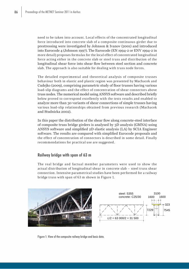
86 Proceedings of the METNET Seminar 2011 in Aarhus
need to be taken into account. Local effects of the concentrated longitudinal force introduced into concrete slab of a composite continuous girder due to prestressing were investigated by Johnson & Ivanov (2001) and introduced into Eurocode 4 (Johnson 1997). The Eurocode (EN 1994-2 or ENV 1994-2 in more detail) proposes formulas for the local effect of concentrated longitudinal force acting either in the concrete slab or steel truss and distribution of the longitudinal shear force into shear flow between steel section and concrete slab. The approach is also suitable for dealing with truss node forces.
The detailed experimental and theoretical analysis of composite trusses behaviour both in elastic and plastic region was presented by Machacek and Cudejko (2009), comprising parametric study of floor trusses having various load-slip diagrams and the effect of concentration of shear connectors above truss nodes. The numerical model using ANSYS software and described briefly below proved to correspond excellently with the tests results and enabled to analyze more than 30 variants of shear connections of simple trusses having various load-slip relationships obtained from previous research (Machacek and Studnicka 2002).
In this paper the distribution of the shear flow along concrete-steel interface of composite truss bridge girders is analysed by 3D analysis (GMNA) using ANSYS software and simplified 2D elastic analysis (LA) by SCIA Engineer software. The results are compared with simplified Eurocode proposals and the effect of concentration of connectors is described in some detail. Finally recommendations for practical use are suggested.
Railway bridge with span of 63 m
The real bridge and factual member parameters were used to show the actual distribution of longitudinal shear in concrete slab – steel truss shear connection. Intensive parametrical studies have been performed for a railway bridge truss with span of 63 m shown in Figure 1.
concrete slab or steel truss and distribution of the longitudinal shear force into shear flow between steel section and concrete slab. The approach is also suitable for dealing with truss node forces. The detailed experimental and theoretical analysis of composite trusses behaviour both in elastic and plastic region was presented by Machacek and Cudejko (2009), comprising parametric study of floor trusses having various load-slip diagrams and the effect of concentration of shear connectors above truss nodes. The numerical model using ANSYS software and described briefly below proved to correspond excellently with the tests results and enabled to analyze more than 30 variants of shear connections of simple trusses having various load-slip relationships obtained from previous research (Machacek and Studnicka 2002). In this paper the distribution of the shear flow along concrete-steel interface of composite truss bridge girders is analysed by 3D analysis (GMNA) using ANSYS software and simplified 2D elastic analysis (LA) by SCIA Engineer software. The results are compared with simplified Eurocode proposals and the effect of concentration of connectors is described in some detail. Finally recommendations for practical use are suggested. Railway bridge with span of 63 m The real bridge and factual member parameters were used to show the actual distribution of longitudinal shear in concrete slab – steel truss shear connection. Intensive parametrical studies have been performed for a railway bridge truss with span of 63 m shown in Figure 1.
L/2 = 63 000/2 = 31 500
7545
323
16003100
1600
7229
steel: S355concrete: C25/30
Figure 1: View of the composite railway bridge and basic data. The area and second moment of area of upper steel flange (with shape) are Au = 0.0390 m2 and Iu = 0.000755 m4 while variable for bottom one from Ab = 0.0328 to 0.0518 m2 and Ib = 0.000944 to 0.001524 m4, for web members from Aw = 0.0448 to 0.0214 m2 and Iw = 0.000708 to 0.000137 m4. Usual modular ratio for short-term loading n0 = Ea/Ecm = 6.89 was accepted if required. Headed studs with 19 mm diameter and ultimate strength fu = 450 MPa located in 4 parallel rows and longitudinally in distance of 400 mm were considered in the study as a basic arrangement, giving characteristic shear strength 4x91400/400 = 914 N/mm, while full shear connection ranges from 809 N/mm to 1023 N/mm (considering non-uniform chord cross section and taking fy into account). The load-slip diagram of shear connectors from study by Oehlers and Coughlan (1986) were employed, see Figure 2.
Figure 1: View of the composite railway bridge and basic data.
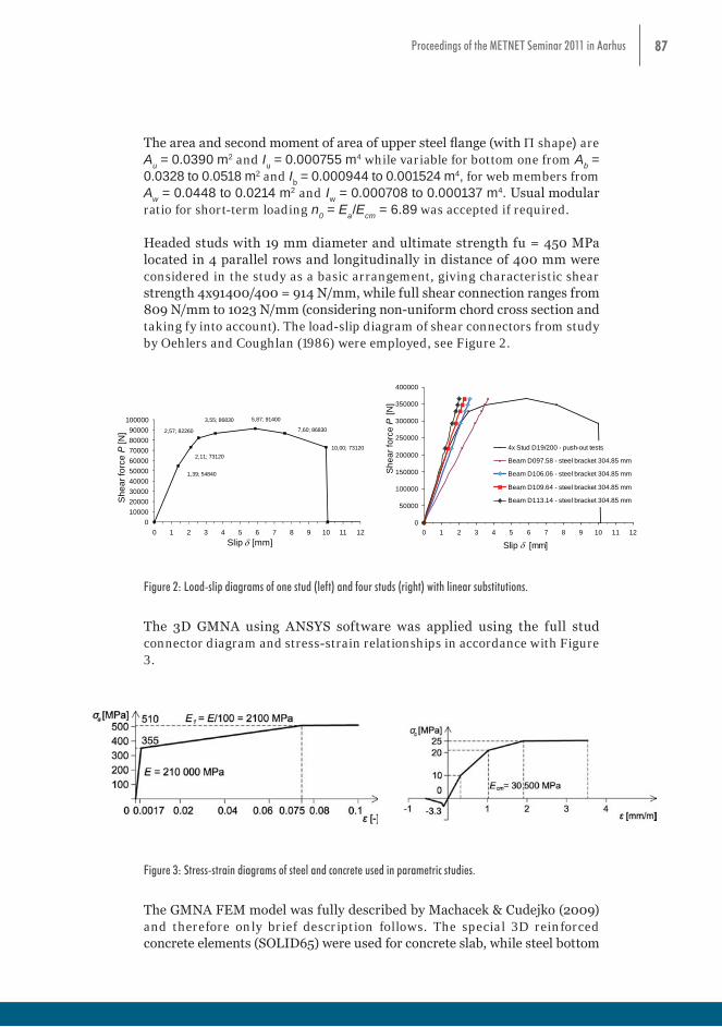
87Proceedings of the METNET Seminar 2011 in Aarhus
The area and second moment of area of upper steel flange (with P shape) are Au = 0.0390 m2 and Iu = 0.000755 m4 while variable for bottom one from Ab = 0.0328 to 0.0518 m2 and Ib = 0.000944 to 0.001524 m4, for web members from Aw = 0.0448 to 0.0214 m2 and Iw = 0.000708 to 0.000137 m4. Usual modular ratio for short-term loading n0 = Ea/Ecm = 6.89 was accepted if required.
Headed studs with 19 mm diameter and ultimate strength fu = 450 MPa located in 4 parallel rows and longitudinally in distance of 400 mm were considered in the study as a basic arrangement, giving characteristic shear strength 4x91400/400 = 914 N/mm, while full shear connection ranges from 809 N/mm to 1023 N/mm (considering non-uniform chord cross section and taking fy into account). The load-slip diagram of shear connectors from study by Oehlers and Coughlan (1986) were employed, see Figure 2.
1,39; 54840
2,11; 73120
2,57; 82260
3,55; 86830 5,87; 91400
7,60; 86830
10,00; 73120
0100002000030000400005000060000700008000090000
100000
0 1 2 3 4 5 6 7 8 9 10 11 12
She
ar fo
rce P
[N]
Slip [mm]
0
50000
100000
150000
200000
250000
300000
350000
400000
0 1 2 3 4 5 6 7 8 9 10 11 12
Slip [mm]
Shea
r for
ce P
[N]
4x Stud D19/200 - push-out tests
Beam D097.58 - steel bracket 304.85 mm
Beam D106.06 - steel bracket 304.85 mm
Beam D109.64 - steel bracket 304.85 mm
Beam D113.14 - steel bracket 304.85 mm
Figure 2: Load-slip diagrams of one stud (left) and four studs (right) with linear substitutions. The 3D GMNA using ANSYS software was applied using the full stud connector diagram and stress-strain relationships in accordance with Figure 3.
Figure 3: Stress-strain diagrams of steel and concrete used in parametric studies.
The GMNA FEM model was fully described by Machacek & Cudejko (2009) and therefore only brief description follows. The special 3D reinforced concrete elements (SOLID65) were used for concrete slab, while steel bottom chord and web bars were modelled by beam elements with appropriate cross section (BEAM24) and upper chord of the steel trusses was composed of shell elements (SHELL43). All steel finite elements enable elastic-plastic analysis (furthermore with large deflections), concrete elements involve smeared reinforcement, crushing and cracking (for shear transfer in opened and closed cracks ANSYS coefficients C1 = 0.3, C2 = 0.6 were used). Shear connection was modelled by non-linear springs located uniformly in required distance along span and placed at a suitable spot between the anticipated shear connector and concrete slab (e.g. at the centre of gravity of holes in perforated shear connector or at base position of headed studs). Nonlinear two node spring element COMBIN39 was employed which makes possible any nonlinear relation between force and extension to model correctly shear forces in direction of girder axis. Vertical and transverse displacements of concrete slab (perpendicular to the girder axis) at springs positions were defined being the same as for the shear connector/steel flange (i.e. no uplift effects were considered). The model was applied to experimental trusses employing real steel and concrete properties and load-slip diagram of used perforated shear connector. Both numerical and experimental central deflections and slips between steel truss and concrete parts were nearly identical and therefore the model may be considered as a benchmark for other models. In the following studies only uniformly distributed loading over span was considered, despite various traffic actions and their combinations in real bridges (e. g. moving local one over bridge deck) with primary interest in transmission of loading in truss nodes. In
Figure 2: Load-slip diagrams of one stud (left) and four studs (right) with linear substitutions.
The 3D GMNA using ANSYS software was applied using the full stud connector diagram and stress-strain relationships in accordance with Figure 3.
1,39; 54840
2,11; 73120
2,57; 82260
3,55; 86830 5,87; 91400
7,60; 86830
10,00; 73120
0100002000030000400005000060000700008000090000
100000
0 1 2 3 4 5 6 7 8 9 10 11 12
She
ar fo
rce P
[N]
Slip [mm]
0
50000
100000
150000
200000
250000
300000
350000
400000
0 1 2 3 4 5 6 7 8 9 10 11 12
Slip [mm]
Shea
r for
ce P
[N]
4x Stud D19/200 - push-out tests
Beam D097.58 - steel bracket 304.85 mm
Beam D106.06 - steel bracket 304.85 mm
Beam D109.64 - steel bracket 304.85 mm
Beam D113.14 - steel bracket 304.85 mm
Figure 2: Load-slip diagrams of one stud (left) and four studs (right) with linear substitutions. The 3D GMNA using ANSYS software was applied using the full stud connector diagram and stress-strain relationships in accordance with Figure 3.
Figure 3: Stress-strain diagrams of steel and concrete used in parametric studies.
The GMNA FEM model was fully described by Machacek & Cudejko (2009) and therefore only brief description follows. The special 3D reinforced concrete elements (SOLID65) were used for concrete slab, while steel bottom chord and web bars were modelled by beam elements with appropriate cross section (BEAM24) and upper chord of the steel trusses was composed of shell elements (SHELL43). All steel finite elements enable elastic-plastic analysis (furthermore with large deflections), concrete elements involve smeared reinforcement, crushing and cracking (for shear transfer in opened and closed cracks ANSYS coefficients C1 = 0.3, C2 = 0.6 were used). Shear connection was modelled by non-linear springs located uniformly in required distance along span and placed at a suitable spot between the anticipated shear connector and concrete slab (e.g. at the centre of gravity of holes in perforated shear connector or at base position of headed studs). Nonlinear two node spring element COMBIN39 was employed which makes possible any nonlinear relation between force and extension to model correctly shear forces in direction of girder axis. Vertical and transverse displacements of concrete slab (perpendicular to the girder axis) at springs positions were defined being the same as for the shear connector/steel flange (i.e. no uplift effects were considered). The model was applied to experimental trusses employing real steel and concrete properties and load-slip diagram of used perforated shear connector. Both numerical and experimental central deflections and slips between steel truss and concrete parts were nearly identical and therefore the model may be considered as a benchmark for other models. In the following studies only uniformly distributed loading over span was considered, despite various traffic actions and their combinations in real bridges (e. g. moving local one over bridge deck) with primary interest in transmission of loading in truss nodes. In
Figure 3: Stress-strain diagrams of steel and concrete used in parametric studies.
The GMNA FEM model was fully described by Machacek & Cudejko (2009) and therefore only brief description follows. The special 3D reinforced concrete elements (SOLID65) were used for concrete slab, while steel bottom
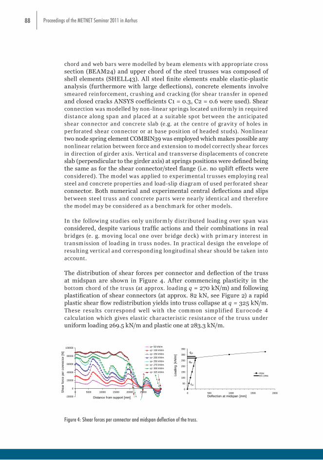
88 Proceedings of the METNET Seminar 2011 in Aarhus
chord and web bars were modelled by beam elements with appropriate cross section (BEAM24) and upper chord of the steel trusses was composed of shell elements (SHELL43). All steel finite elements enable elastic-plastic analysis (furthermore with large deflections), concrete elements involve smeared reinforcement, crushing and cracking (for shear transfer in opened and closed cracks ANSYS coefficients C1 = 0.3, C2 = 0.6 were used). Shear connection was modelled by non-linear springs located uniformly in required distance along span and placed at a suitable spot between the anticipated shear connector and concrete slab (e.g. at the centre of gravity of holes in perforated shear connector or at base position of headed studs). Nonlinear two node spring element COMBIN39 was employed which makes possible any nonlinear relation between force and extension to model correctly shear forces in direction of girder axis. Vertical and transverse displacements of concrete slab (perpendicular to the girder axis) at springs positions were defined being the same as for the shear connector/steel flange (i.e. no uplift effects were considered). The model was applied to experimental trusses employing real steel and concrete properties and load-slip diagram of used perforated shear connector. Both numerical and experimental central deflections and slips between steel truss and concrete parts were nearly identical and therefore the model may be considered as a benchmark for other models.
In the following studies only uniformly distributed loading over span was considered, despite various traffic actions and their combinations in real bridges (e. g. moving local one over bridge deck) with primary interest in transmission of loading in truss nodes. In practical design the envelope of resulting vertical and corresponding longitudinal shear should be taken into account.
The distribution of shear forces per connector and deflection of the truss at midspan are shown in Figure 4. After commencing plasticity in the bottom chord of the truss (at approx. loading q = 270 kN/m) and following plastification of shear connectors (at approx. 82 kN, see Figure 2) a rapid plastic shear flow redistribution yields into truss collapse at q = 325 kN/m. These results correspond well with the common simplified Eurocode 4 calculation which gives elastic characteristic resistance of the truss under uniform loading 269.5 kN/m and plastic one at 283.3 kN/m.
practical design the envelope of resulting vertical and corresponding longitudinal shear should be taken into account. The distribution of shear forces per connector and deflection of the truss at midspan are shown in Figure 4. After commencing plasticity in the bottom chord of the truss (at approx. loading q = 270 kN/m) and following plastification of shear connectors (at approx. 82 kN, see Figure 2) a rapid plastic shear flow redistribution yields into truss collapse at q = 325 kN/m. These results correspond well with the common simplified Eurocode 4 calculation which gives elastic characteristic resistance of the truss under uniform loading 269.5 kN/m and plastic one at 283.3 kN/m.
-20000
0
20000
40000
60000
80000
100000
0 5000 10000 15000 20000 25000 30000
Distance from support [mm]
Shea
r for
ce p
er c
onne
ctor
[N]
q= 50 kN/mq= 100 kN/mq= 150 kN/mq= 200 kN/mq= 250 kN/mq= 270 kN/mq= 300 kN/mq= 325 kN/m
0
50
100
150
200
250
300
350
0 500 1000 1500 2000
Load
ing
[kN
/m]
Deflection at midspan [mm]
FEMEN 1994
qpl
qel
δel
Figure 4: Shear forces per connector and midspan deflection of the truss.
Due to very demanding GMNA by ANSYS another study using simplified 2D LA with help of SCIA Engineer common frame software modelling shear connection as short cantilevers between steel truss and concrete slab was performed. Only first linear parts of the relationships for both steel and concrete (Young’s modulus E, Ecm) and compressed linear diagrams representing 4 studs per row in accordance with Figure 2 in the right were employed. The shear connectors were modelled as cantilevers of length 304.85 mm sticking out from steel flange axis and pin connected at midplane of concrete slab represented by a concrete strut (neglecting slab tension zone) see Figure 5. Such approach, of course, relates to study of longitudinal shear only.
305concrete slab
member representing concrete slab
steel flange
member representing steel chordin compression chord axis
DD
Figure 5: 2D model of shear connection. The beam D109.64 has top cantilever rigidity identical with the first linear part of the load-slip diagram (Figure 2) and the number corresponds to fictitious stud-cantilever diameter D = 109.64 mm. The simplified elastic linear analysis (SCIA) under loading 200 kN/m (which is near to design bridge loading) gives shear forces as shown in Figure 6 and compared with the above 3D GMNA analysis. The simplified analysis reasonably imitates the ANSYS analysis, while conservativeness (higher values in shear peaks) of simplified elastic solution is obvious.
Figure 4: Shear forces per connector and midspan deflection of the truss.
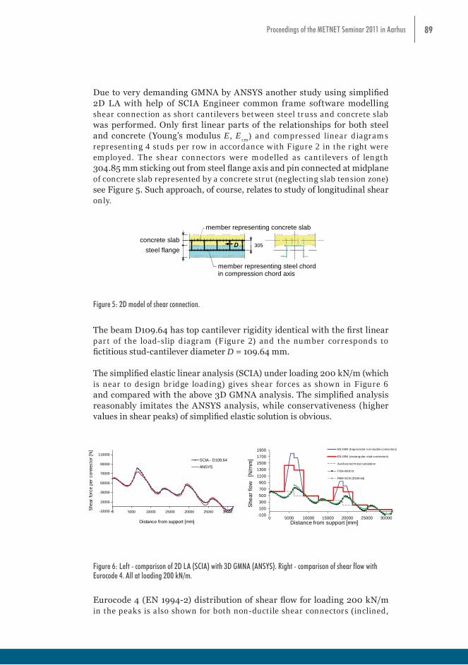
89Proceedings of the METNET Seminar 2011 in Aarhus
Due to very demanding GMNA by ANSYS another study using simplified 2D LA with help of SCIA Engineer common frame software modelling shear connection as short cantilevers between steel truss and concrete slab was performed. Only first linear parts of the relationships for both steel and concrete (Young’s modulus E, E
cm) and compressed linear diagrams
representing 4 studs per row in accordance with Figure 2 in the right were employed. The shear connectors were modelled as cantilevers of length 304.85 mm sticking out from steel flange axis and pin connected at midplane of concrete slab represented by a concrete strut (neglecting slab tension zone) see Figure 5. Such approach, of course, relates to study of longitudinal shear only.
practical design the envelope of resulting vertical and corresponding longitudinal shear should be taken into account. The distribution of shear forces per connector and deflection of the truss at midspan are shown in Figure 4. After commencing plasticity in the bottom chord of the truss (at approx. loading q = 270 kN/m) and following plastification of shear connectors (at approx. 82 kN, see Figure 2) a rapid plastic shear flow redistribution yields into truss collapse at q = 325 kN/m. These results correspond well with the common simplified Eurocode 4 calculation which gives elastic characteristic resistance of the truss under uniform loading 269.5 kN/m and plastic one at 283.3 kN/m.
-20000
0
20000
40000
60000
80000
100000
0 5000 10000 15000 20000 25000 30000
Distance from support [mm]
Shea
r for
ce p
er c
onne
ctor
[N]
q= 50 kN/mq= 100 kN/mq= 150 kN/mq= 200 kN/mq= 250 kN/mq= 270 kN/mq= 300 kN/mq= 325 kN/m
0
50
100
150
200
250
300
350
0 500 1000 1500 2000
Load
ing
[kN
/m]
Deflection at midspan [mm]
FEMEN 1994
qpl
qel
δel
Figure 4: Shear forces per connector and midspan deflection of the truss.
Due to very demanding GMNA by ANSYS another study using simplified 2D LA with help of SCIA Engineer common frame software modelling shear connection as short cantilevers between steel truss and concrete slab was performed. Only first linear parts of the relationships for both steel and concrete (Young’s modulus E, Ecm) and compressed linear diagrams representing 4 studs per row in accordance with Figure 2 in the right were employed. The shear connectors were modelled as cantilevers of length 304.85 mm sticking out from steel flange axis and pin connected at midplane of concrete slab represented by a concrete strut (neglecting slab tension zone) see Figure 5. Such approach, of course, relates to study of longitudinal shear only.
305concrete slab
member representing concrete slab
steel flange
member representing steel chordin compression chord axis
DD
Figure 5: 2D model of shear connection. The beam D109.64 has top cantilever rigidity identical with the first linear part of the load-slip diagram (Figure 2) and the number corresponds to fictitious stud-cantilever diameter D = 109.64 mm. The simplified elastic linear analysis (SCIA) under loading 200 kN/m (which is near to design bridge loading) gives shear forces as shown in Figure 6 and compared with the above 3D GMNA analysis. The simplified analysis reasonably imitates the ANSYS analysis, while conservativeness (higher values in shear peaks) of simplified elastic solution is obvious.
Figure 5: 2D model of shear connection.
The beam D109.64 has top cantilever rigidity identical with the first linear part of the load-slip diagram (Figure 2) and the number corresponds to fictitious stud-cantilever diameter D = 109.64 mm.
The simplified elastic linear analysis (SCIA) under loading 200 kN/m (which is near to design bridge loading) gives shear forces as shown in Figure 6 and compared with the above 3D GMNA analysis. The simplified analysis reasonably imitates the ANSYS analysis, while conservativeness (higher values in shear peaks) of simplified elastic solution is obvious.
-10000
10000
30000
50000
70000
90000
110000
0 5000 10000 15000 20000 25000 30000
Distance from support [mm]
Shea
r for
ce p
er c
onne
ctor
[N]
SCIA - D109.64
ANSYS
Figure 6: Left - comparison of 2D LA (SCIA) with 3D GMNA (ANSYS).
Right - comparison of shear flow with Eurocode 4. All at loading 200 kN/m. Eurocode 4 (EN 1994-2) distribution of shear flow for loading 200 kN/m in the peaks is also shown for both non-ductile shear connectors (inclined, trapezoidal distribution) and ductile ones (rectangular distribution) in Figure 6. The local shear in accordance with the Eurocode is distributed on the length Lv = ed + beff = (1500 + 2 x 148.5) + 3150 = 4947 mm and gives very conservative values. The decisive role plays the effective width beff, which is limited by the concrete slab width available. It should be mentioned that the length for local shear distribution in the Eurocode resulted from brilliant 3D elastic studies (Johnson and Ivanov 2001) but apparently after abnormal simplification. Results of study concerning shear connection rigidity are presented in Figure 7. With rigidities in accordance to Figure 2, where D106.06 and D097.58 are less stiff, the lowering of shear peaks is obvious.
-10000
10000
30000
50000
70000
90000
110000
0 5000 10000 15000 20000 25000 30000
Distance from support [mm]
Shea
r for
ce p
er c
onne
ctor
[N]
D097.58
D106.06
D109.64
D113.14
Figure 7: Influence of shear connection rigidity (2D LA - SCIA), q = 200 kN/m.
Road bridge without gusset plates with span of 21 m Composite truss bridge without gusset plates common in Central Europe as a motorway or river overbridge was investigated. Only modification of a real application (which is usually fixed at the stiff support blocks and has more diagonals) is shown in Figure 8. The span of the truss is 21 m and steel members are from flats only [mm]: upper flange 250x20, diagonals 250x40, bottom flange 300x40. Headed studs with 19 mm diameter and fu = 340 MPa located in 3 parallel rows and longitudinally in distance of 200 mm were considered for shear connection, giving characteristic shear strength 3x77100/200 = 1156 N/mm, which represents full shear connection (the bridge parameters give the required shear flow Nc,f = Aafy/0.5L = 575 N/mm, taking yield stress fy into account) as required for bridges.
-100100300500700900
11001300150017001900
0 5000 10000 15000 20000 25000 30000
She
ar fl
ow
[N/m
m]
Distance from support [mm]
EN 1994 (trapezoidal: non-ductile connectors)
EN 1994 (rectangular: stud connectors)
Auxiliary technical calculation
FEM-ANSYS
FEM-SCIA (D109.64)
Figure 6: Left - comparison of 2D LA (SCIA) with 3D GMNA (ANSYS). Right - comparison of shear flow with Eurocode 4. All at loading 200 kN/m.
Eurocode 4 (EN 1994-2) distribution of shear flow for loading 200 kN/m in the peaks is also shown for both non-ductile shear connectors (inclined,
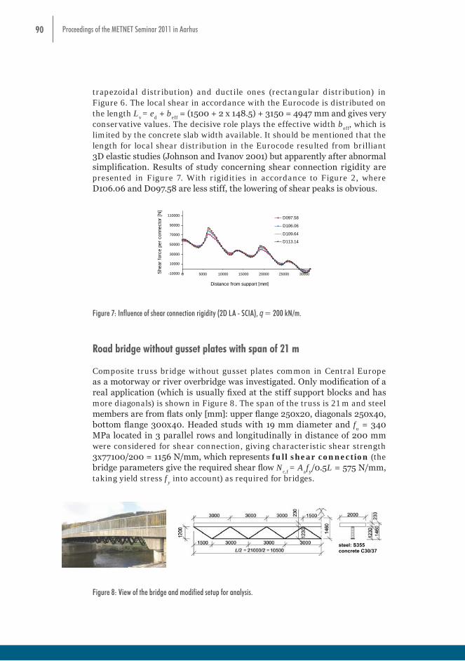
90 Proceedings of the METNET Seminar 2011 in Aarhus
trapezoidal distribution) and ductile ones (rectangular distribution) in Figure 6. The local shear in accordance with the Eurocode is distributed on the length L
v = e
d + b
eff = (1500 + 2 x 148.5) + 3150 = 4947 mm and gives very
conservative values. The decisive role plays the effective width beff
, which is limited by the concrete slab width available. It should be mentioned that the length for local shear distribution in the Eurocode resulted from brilliant 3D elastic studies (Johnson and Ivanov 2001) but apparently after abnormal simplification. Results of study concerning shear connection rigidity are presented in Figure 7. With rigidities in accordance to Figure 2, where D106.06 and D097.58 are less stiff, the lowering of shear peaks is obvious.
-10000
10000
30000
50000
70000
90000
110000
0 5000 10000 15000 20000 25000 30000
Distance from support [mm]
Shea
r for
ce p
er c
onne
ctor
[N]
SCIA - D109.64
ANSYS
Figure 6: Left - comparison of 2D LA (SCIA) with 3D GMNA (ANSYS).
Right - comparison of shear flow with Eurocode 4. All at loading 200 kN/m. Eurocode 4 (EN 1994-2) distribution of shear flow for loading 200 kN/m in the peaks is also shown for both non-ductile shear connectors (inclined, trapezoidal distribution) and ductile ones (rectangular distribution) in Figure 6. The local shear in accordance with the Eurocode is distributed on the length Lv = ed + beff = (1500 + 2 x 148.5) + 3150 = 4947 mm and gives very conservative values. The decisive role plays the effective width beff, which is limited by the concrete slab width available. It should be mentioned that the length for local shear distribution in the Eurocode resulted from brilliant 3D elastic studies (Johnson and Ivanov 2001) but apparently after abnormal simplification. Results of study concerning shear connection rigidity are presented in Figure 7. With rigidities in accordance to Figure 2, where D106.06 and D097.58 are less stiff, the lowering of shear peaks is obvious.
-10000
10000
30000
50000
70000
90000
110000
0 5000 10000 15000 20000 25000 30000
Distance from support [mm]
Shea
r for
ce p
er c
onne
ctor
[N]
D097.58
D106.06
D109.64
D113.14
Figure 7: Influence of shear connection rigidity (2D LA - SCIA), q = 200 kN/m.
Road bridge without gusset plates with span of 21 m Composite truss bridge without gusset plates common in Central Europe as a motorway or river overbridge was investigated. Only modification of a real application (which is usually fixed at the stiff support blocks and has more diagonals) is shown in Figure 8. The span of the truss is 21 m and steel members are from flats only [mm]: upper flange 250x20, diagonals 250x40, bottom flange 300x40. Headed studs with 19 mm diameter and fu = 340 MPa located in 3 parallel rows and longitudinally in distance of 200 mm were considered for shear connection, giving characteristic shear strength 3x77100/200 = 1156 N/mm, which represents full shear connection (the bridge parameters give the required shear flow Nc,f = Aafy/0.5L = 575 N/mm, taking yield stress fy into account) as required for bridges.
-100100300500700900
11001300150017001900
0 5000 10000 15000 20000 25000 30000
She
ar fl
ow
[N/m
m]
Distance from support [mm]
EN 1994 (trapezoidal: non-ductile connectors)
EN 1994 (rectangular: stud connectors)
Auxiliary technical calculation
FEM-ANSYS
FEM-SCIA (D109.64)
Figure 7: Influence of shear connection rigidity (2D LA - SCIA), q = 200 kN/m.
Road bridge without gusset plates with span of 21 m
Composite truss bridge without gusset plates common in Central Europe as a motorway or river overbridge was investigated. Only modification of a real application (which is usually fixed at the stiff support blocks and has more diagonals) is shown in Figure 8. The span of the truss is 21 m and steel members are from flats only [mm]: upper flange 250x20, diagonals 250x40, bottom flange 300x40. Headed studs with 19 mm diameter and f
u = 340
MPa located in 3 parallel rows and longitudinally in distance of 200 mm were considered for shear connection, giving characteristic shear strength 3x77100/200 = 1156 N/mm, which represents full shear connection (the bridge parameters give the required shear flow N
c,f = A
af
y/0.5L = 575 N/mm,
taking yield stress fy into account) as required for bridges.
Figure 8: View of the bridge and modified setup for analysis.
Again, the shear forces in shear connectors resulting from the 3D GMNA using ANSYS software are shown for one half of the truss girder and the curves show values for load steps increasing up to the numerical collapse value given by maximal value in captions, Figure 9 (half span shown).
Figure 9: Load-slip diagrams of one stud (left) and shear forces in connectors (right).
Analysis with decreased shear connection strength to 70 % with value of 809 N/mm (note that the value still ensures the full shear connection) to find out influence of connection rigidity is presented in Figure 10.
0,10; 27615
4,00; 53970
0100002000030000400005000060000700008000090000
0 1 2 3 4 5 6 7 8 9 10 11
She
ar fo
rce P
[N]
Slip [mm]
Figure 10: As in Figure 9 but connection rigidity reduced to 70 %.
Less distinctive shear peaks were found accompanied by some decrease of collapse load in comparison to former connection (note that Eurocode 4 plastic resistance corresponds to 112,5 kN/m, elastic one to 102,0 kN/m, for fabrication with propping), which is due to final plastic redistribution of shear forces in extremely loaded shear connectors near support. Shear flow according to numerical FEM and simplified Standard procedure (EN 1994-2) for loading 75 kN/m (near the design loading) is shown in Figure 11. Within the Eurocode approach the effective width available (beff = 2 m) and twice the half flange depth ed = 2ev = 20 mm (because of no gusset plates) in accordance with the Standard were applied.
steel: S355 concrete C30/37
0,10; 39450
4,00; 77100
0100002000030000400005000060000700008000090000
0 1 2 3 4 5 6 7 8 9 10 11
Shea
r for
ce P
[N]
Slip [mm]
-50005000
1500025000350004500055000650007500085000
0 1500 3000 4500 6000 7500 9000 10500Shea
r fo
rce
per
conn
ecto
r [N
]
Distance from support [mm]
q= 15 kN/m
q= 30 kN/m
q= 45 kN/m
q= 60 kN/m
q= 75 kN/m
q= 90 kN/m
q= 105 kN/m
q= 122 kN/m
-50005000
1500025000350004500055000650007500085000
0 1500 3000 4500 6000 7500 9000 10500Shea
r fo
rce
per
conn
ecto
r [N
]
Distance from support [mm]
q= 15 kN/m
q= 30 kN/m
q= 45 kN/m
q= 60 kN/m
q= 75 kN/m
q= 90 kN/m
q= 105 kN/m
q= 115 kN/m
Figure 8: View of the bridge and modified setup for analysis.
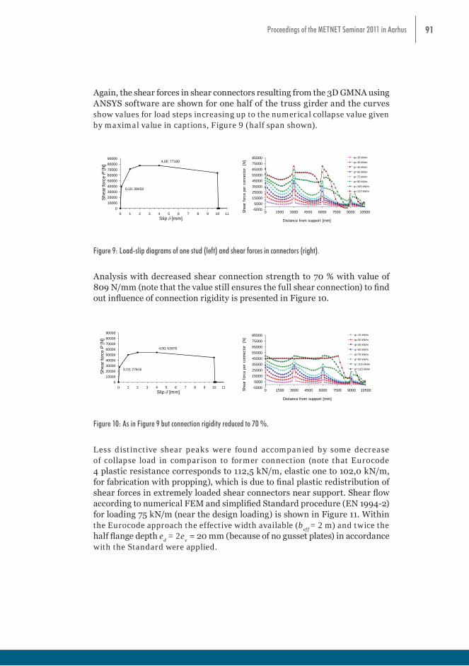
91Proceedings of the METNET Seminar 2011 in Aarhus
Again, the shear forces in shear connectors resulting from the 3D GMNA using ANSYS software are shown for one half of the truss girder and the curves show values for load steps increasing up to the numerical collapse value given by maximal value in captions, Figure 9 (half span shown).
Figure 8: View of the bridge and modified setup for analysis.
Again, the shear forces in shear connectors resulting from the 3D GMNA using ANSYS software are shown for one half of the truss girder and the curves show values for load steps increasing up to the numerical collapse value given by maximal value in captions, Figure 9 (half span shown).
Figure 9: Load-slip diagrams of one stud (left) and shear forces in connectors (right).
Analysis with decreased shear connection strength to 70 % with value of 809 N/mm (note that the value still ensures the full shear connection) to find out influence of connection rigidity is presented in Figure 10.
0,10; 27615
4,00; 53970
0100002000030000400005000060000700008000090000
0 1 2 3 4 5 6 7 8 9 10 11
She
ar fo
rce P
[N]
Slip [mm]
Figure 10: As in Figure 9 but connection rigidity reduced to 70 %.
Less distinctive shear peaks were found accompanied by some decrease of collapse load in comparison to former connection (note that Eurocode 4 plastic resistance corresponds to 112,5 kN/m, elastic one to 102,0 kN/m, for fabrication with propping), which is due to final plastic redistribution of shear forces in extremely loaded shear connectors near support. Shear flow according to numerical FEM and simplified Standard procedure (EN 1994-2) for loading 75 kN/m (near the design loading) is shown in Figure 11. Within the Eurocode approach the effective width available (beff = 2 m) and twice the half flange depth ed = 2ev = 20 mm (because of no gusset plates) in accordance with the Standard were applied.
steel: S355 concrete C30/37
0,10; 39450
4,00; 77100
0100002000030000400005000060000700008000090000
0 1 2 3 4 5 6 7 8 9 10 11
Shea
r for
ce P
[N]
Slip [mm]
-50005000
1500025000350004500055000650007500085000
0 1500 3000 4500 6000 7500 9000 10500Shea
r fo
rce
per
conn
ecto
r [N
]
Distance from support [mm]
q= 15 kN/m
q= 30 kN/m
q= 45 kN/m
q= 60 kN/m
q= 75 kN/m
q= 90 kN/m
q= 105 kN/m
q= 122 kN/m
-50005000
1500025000350004500055000650007500085000
0 1500 3000 4500 6000 7500 9000 10500Shea
r fo
rce
per
conn
ecto
r [N
]
Distance from support [mm]
q= 15 kN/m
q= 30 kN/m
q= 45 kN/m
q= 60 kN/m
q= 75 kN/m
q= 90 kN/m
q= 105 kN/m
q= 115 kN/m
Figure 9: Load-slip diagrams of one stud (left) and shear forces in connectors (right).
Analysis with decreased shear connection strength to 70 % with value of 809 N/mm (note that the value still ensures the full shear connection) to find out influence of connection rigidity is presented in Figure 10.
Figure 8: View of the bridge and modified setup for analysis.
Again, the shear forces in shear connectors resulting from the 3D GMNA using ANSYS software are shown for one half of the truss girder and the curves show values for load steps increasing up to the numerical collapse value given by maximal value in captions, Figure 9 (half span shown).
Figure 9: Load-slip diagrams of one stud (left) and shear forces in connectors (right).
Analysis with decreased shear connection strength to 70 % with value of 809 N/mm (note that the value still ensures the full shear connection) to find out influence of connection rigidity is presented in Figure 10.
0,10; 27615
4,00; 53970
0100002000030000400005000060000700008000090000
0 1 2 3 4 5 6 7 8 9 10 11
She
ar fo
rce P
[N]
Slip [mm]
Figure 10: As in Figure 9 but connection rigidity reduced to 70 %.
Less distinctive shear peaks were found accompanied by some decrease of collapse load in comparison to former connection (note that Eurocode 4 plastic resistance corresponds to 112,5 kN/m, elastic one to 102,0 kN/m, for fabrication with propping), which is due to final plastic redistribution of shear forces in extremely loaded shear connectors near support. Shear flow according to numerical FEM and simplified Standard procedure (EN 1994-2) for loading 75 kN/m (near the design loading) is shown in Figure 11. Within the Eurocode approach the effective width available (beff = 2 m) and twice the half flange depth ed = 2ev = 20 mm (because of no gusset plates) in accordance with the Standard were applied.
steel: S355 concrete C30/37
0,10; 39450
4,00; 77100
0100002000030000400005000060000700008000090000
0 1 2 3 4 5 6 7 8 9 10 11
Shea
r for
ce P
[N]
Slip [mm]
-50005000
1500025000350004500055000650007500085000
0 1500 3000 4500 6000 7500 9000 10500Shea
r fo
rce
per
conn
ecto
r [N
]
Distance from support [mm]
q= 15 kN/m
q= 30 kN/m
q= 45 kN/m
q= 60 kN/m
q= 75 kN/m
q= 90 kN/m
q= 105 kN/m
q= 122 kN/m
-50005000
1500025000350004500055000650007500085000
0 1500 3000 4500 6000 7500 9000 10500Shea
r fo
rce
per
conn
ecto
r [N
]
Distance from support [mm]
q= 15 kN/m
q= 30 kN/m
q= 45 kN/m
q= 60 kN/m
q= 75 kN/m
q= 90 kN/m
q= 105 kN/m
q= 115 kN/m
Figure 10: As in Figure 9 but connection rigidity reduced to 70 %.
Less distinctive shear peaks were found accompanied by some decrease of collapse load in comparison to former connection (note that Eurocode 4 plastic resistance corresponds to 112,5 kN/m, elastic one to 102,0 kN/m, for fabrication with propping), which is due to final plastic redistribution of shear forces in extremely loaded shear connectors near support. Shear flow according to numerical FEM and simplified Standard procedure (EN 1994-2) for loading 75 kN/m (near the design loading) is shown in Figure 11. Within the Eurocode approach the effective width available (b
eff = 2 m) and twice the
half flange depth ed = 2e
v = 20 mm (because of no gusset plates) in accordance
with the Standard were applied.
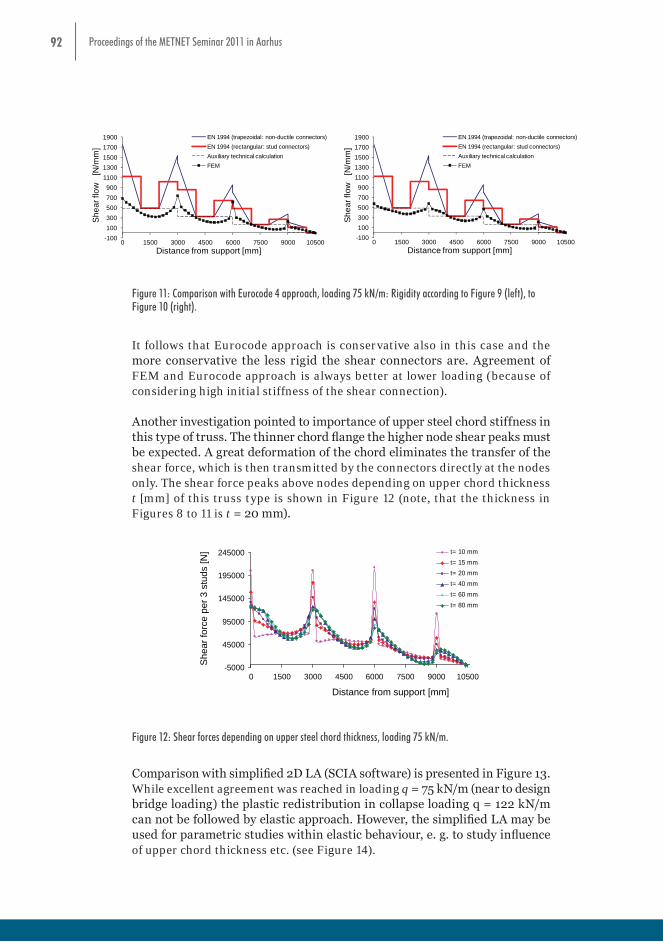
92 Proceedings of the METNET Seminar 2011 in Aarhus
-100100300500700900
11001300150017001900
0 1500 3000 4500 6000 7500 9000 10500
Shea
r flo
w
[N/m
m]
Distance from support [mm]
EN 1994 (trapezoidal: non-ductile connectors)EN 1994 (rectangular: stud connectors)Auxiliary technical calculationFEM
-100100300500700900
11001300150017001900
0 1500 3000 4500 6000 7500 9000 10500
Shea
r flo
w
[N/m
m]
Distance from support [mm]
EN 1994 (trapezoidal: non-ductile connectors)EN 1994 (rectangular: stud connectors)Auxiliary technical calculationFEM
Figure 11: Comparison with Eurocode 4 approach, loading 75 kN/m:
Rigidity according to Figure 9 (left), to Figure 10 (right). It follows that Eurocode approach is conservative also in this case and the more conservative the less rigid the shear connectors are. Agreement of FEM and Eurocode approach is always better at lower loading (because of considering high initial stiffness of the shear connection). Another investigation pointed to importance of upper steel chord stiffness in this type of truss. The thinner chord flange the higher node shear peaks must be expected. A great deformation of the chord eliminates the transfer of the shear force, which is then transmitted by the connectors directly at the nodes only. The shear force peaks above nodes depending on upper chord thickness t [mm] of this truss type is shown in Figure 12 (note, that the thickness in Figures 8 to 11 is t = 20 mm).
Figure 12: Shear forces depending on upper steel chord thickness, loading 75 kN/m. Comparison with simplified 2D LA (SCIA software) is presented in Figure 13. While excellent agreement was reached in loading q = 75 kN/m (near to design bridge loading) the plastic redistribution in collapse loading q = 122 kN/m can not be followed by elastic approach. However, the simplified LA may be used for parametric studies within elastic behaviour, e. g. to study influence of upper chord thickness etc. (see Figure 14).
-5000
45000
95000
145000
195000
245000
0 1500 3000 4500 6000 7500 9000 10500Vzdálenost od podpory [mm]
Sm
ykov
á sí
la [N
]
t= 10 mmt= 15 mmt= 20 mmt= 40 mmt= 60 mmt= 80 mm
She
ar fo
rce
per 3
stu
ds [N
]
Distance from support [mm]
Figure 11: Comparison with Eurocode 4 approach, loading 75 kN/m: Rigidity according to Figure 9 (left), to Figure 10 (right).
It follows that Eurocode approach is conservative also in this case and the more conservative the less rigid the shear connectors are. Agreement of FEM and Eurocode approach is always better at lower loading (because of considering high initial stiffness of the shear connection).
Another investigation pointed to importance of upper steel chord stiffness in this type of truss. The thinner chord flange the higher node shear peaks must be expected. A great deformation of the chord eliminates the transfer of the shear force, which is then transmitted by the connectors directly at the nodes only. The shear force peaks above nodes depending on upper chord thickness t [mm] of this truss type is shown in Figure 12 (note, that the thickness in Figures 8 to 11 is t = 20 mm).
-100100300500700900
11001300150017001900
0 1500 3000 4500 6000 7500 9000 10500
Shea
r flo
w
[N/m
m]
Distance from support [mm]
EN 1994 (trapezoidal: non-ductile connectors)EN 1994 (rectangular: stud connectors)Auxiliary technical calculationFEM
-100100300500700900
11001300150017001900
0 1500 3000 4500 6000 7500 9000 10500
Shea
r flo
w
[N/m
m]
Distance from support [mm]
EN 1994 (trapezoidal: non-ductile connectors)EN 1994 (rectangular: stud connectors)Auxiliary technical calculationFEM
Figure 11: Comparison with Eurocode 4 approach, loading 75 kN/m:
Rigidity according to Figure 9 (left), to Figure 10 (right). It follows that Eurocode approach is conservative also in this case and the more conservative the less rigid the shear connectors are. Agreement of FEM and Eurocode approach is always better at lower loading (because of considering high initial stiffness of the shear connection). Another investigation pointed to importance of upper steel chord stiffness in this type of truss. The thinner chord flange the higher node shear peaks must be expected. A great deformation of the chord eliminates the transfer of the shear force, which is then transmitted by the connectors directly at the nodes only. The shear force peaks above nodes depending on upper chord thickness t [mm] of this truss type is shown in Figure 12 (note, that the thickness in Figures 8 to 11 is t = 20 mm).
Figure 12: Shear forces depending on upper steel chord thickness, loading 75 kN/m. Comparison with simplified 2D LA (SCIA software) is presented in Figure 13. While excellent agreement was reached in loading q = 75 kN/m (near to design bridge loading) the plastic redistribution in collapse loading q = 122 kN/m can not be followed by elastic approach. However, the simplified LA may be used for parametric studies within elastic behaviour, e. g. to study influence of upper chord thickness etc. (see Figure 14).
-5000
45000
95000
145000
195000
245000
0 1500 3000 4500 6000 7500 9000 10500Vzdálenost od podpory [mm]
Sm
ykov
á sí
la [N
]
t= 10 mmt= 15 mmt= 20 mmt= 40 mmt= 60 mmt= 80 mm
She
ar fo
rce
per 3
stu
ds [N
]
Distance from support [mm]
Figure 12: Shear forces depending on upper steel chord thickness, loading 75 kN/m.
Comparison with simplified 2D LA (SCIA software) is presented in Figure 13. While excellent agreement was reached in loading q = 75 kN/m (near to design bridge loading) the plastic redistribution in collapse loading q = 122 kN/m can not be followed by elastic approach. However, the simplified LA may be used for parametric studies within elastic behaviour, e. g. to study influence of upper chord thickness etc. (see Figure 14).

93Proceedings of the METNET Seminar 2011 in Aarhus
-5000
5000
15000
25000
35000
45000
55000
65000
75000
85000
0 1500 3000 4500 6000 7500 9000 10500
Distance from support [mm]
Shea
r for
ce p
er c
onne
ctor
[N]
ANSYS
SCIA
-5000
5000
15000
25000
35000
45000
55000
65000
75000
85000
0 1500 3000 4500 6000 7500 9000 10500
Distance from support [mm]
Shea
r for
ce p
er c
onne
ctor
[N]
ANSYS
SCIA
Figure 13: Comparison of 2D LA and 3D GMNA. Loading 75 kN/m (left), collapse loading 122 kN/m (right)
-5000
5000
15000
25000
35000
45000
55000
65000
75000
85000
0 1500 3000 4500 6000 7500 9000 10500
Distance from support [mm]
Shea
r for
ce p
er c
onne
ctor
[N]
ANSYS
SCIA
-5000
5000
15000
25000
35000
45000
55000
65000
75000
85000
0 1500 3000 4500 6000 7500 9000 10500
Distance from support [mm]
Shea
r for
ce p
er c
onne
ctor
[N]
ANSYS
SCIA
Figure 14: Comparison of 2D LA and 3D GMNA, loading q = 75 kN/m. Flange thickness t = 15 mm (left), t = 80 mm (right)
Concentration of shear connectors above truss nodes The peaks of the longitudinal shear in composite trusses makes designers to concentrate shear connectors above truss nodes. While intensive study is under progress the quadruple concentration in three various lengths d and denoted as D1, D2, D3 for the railway bridge shown above is presented here only (Figure 15).
Dd d e ed
L/2 = 63 000/2 = 31 500
Basic arrangement: 4 parallel studs, e = 400 mmConcentration: D1: 4 parallel studs, e = 100 mm, d = D/4 D2: 4 parallel studs, e = 100 mm, d = D/5 D3: 4 parallel studs, e = 100 mm, d = D/6
d
d
d
Figure 15: Geometry of concentrated connectors above truss nodes.
With narrower concentrated area the shear forces per connector are higher (Figure 16) while the increased total shear (sum of the shear forces recalculated to basic arrangement) due to higher shear stiffness above nodes is obvious. Extent d/D ≈ 0.25 (i.e. a quarter of node distance) seems to be optimal. The increase of the total shear flow in the concentrated areas (dotted lines) reached in D1 case 97 % (in D3 even 129 %), accompanied by a corresponding decrease of shear flow (approximately to one half) in non-concentrated regions.
Figure 13: Comparison of 2D LA and 3D GMNA. Loading 75 kN/m (left), collapse loading 122 kN/m (right)
-5000
5000
15000
25000
35000
45000
55000
65000
75000
85000
0 1500 3000 4500 6000 7500 9000 10500
Distance from support [mm]
Shea
r for
ce p
er c
onne
ctor
[N]
ANSYS
SCIA
-5000
5000
15000
25000
35000
45000
55000
65000
75000
85000
0 1500 3000 4500 6000 7500 9000 10500
Distance from support [mm]
Shea
r for
ce p
er c
onne
ctor
[N]
ANSYS
SCIA
Figure 14: Comparison of 2D LA and 3D GMNA, loading q = 75 kN/m. Flange thickness t = 15 mm (left), t = 80 mm (right)
Concentration of shear connectors above truss nodes The peaks of the longitudinal shear in composite trusses makes designers to concentrate shear connectors above truss nodes. While intensive study is under progress the quadruple concentration in three various lengths d and denoted as D1, D2, D3 for the railway bridge shown above is presented here only (Figure 15).
Dd d e ed
L/2 = 63 000/2 = 31 500
Basic arrangement: 4 parallel studs, e = 400 mmConcentration: D1: 4 parallel studs, e = 100 mm, d = D/4 D2: 4 parallel studs, e = 100 mm, d = D/5 D3: 4 parallel studs, e = 100 mm, d = D/6
d
d
d
Figure 15: Geometry of concentrated connectors above truss nodes.
With narrower concentrated area the shear forces per connector are higher (Figure 16) while the increased total shear (sum of the shear forces recalculated to basic arrangement) due to higher shear stiffness above nodes is obvious. Extent d/D ≈ 0.25 (i.e. a quarter of node distance) seems to be optimal. The increase of the total shear flow in the concentrated areas (dotted lines) reached in D1 case 97 % (in D3 even 129 %), accompanied by a corresponding decrease of shear flow (approximately to one half) in non-concentrated regions.
Figure 14: Comparison of 2D LA and 3D GMNA, loading q = 75 kN/m. Flange thickness t = 15 mm (left), t = 80 mm (right)
Concentration of shear connectors above truss nodes
The peaks of the longitudinal shear in composite trusses makes designers to concentrate shear connectors above truss nodes. While intensive study is under progress the quadruple concentration in three various lengths d and denoted as D1, D2, D3 for the railway bridge shown above is presented here only (Figure 15).
-5000
5000
15000
25000
35000
45000
55000
65000
75000
85000
0 1500 3000 4500 6000 7500 9000 10500
Distance from support [mm]
Shea
r for
ce p
er c
onne
ctor
[N]
ANSYS
SCIA
-5000
5000
15000
25000
35000
45000
55000
65000
75000
85000
0 1500 3000 4500 6000 7500 9000 10500
Distance from support [mm]
Shea
r for
ce p
er c
onne
ctor
[N]
ANSYS
SCIA
Figure 13: Comparison of 2D LA and 3D GMNA. Loading 75 kN/m (left), collapse loading 122 kN/m (right)
-5000
5000
15000
25000
35000
45000
55000
65000
75000
85000
0 1500 3000 4500 6000 7500 9000 10500
Distance from support [mm]
Shea
r for
ce p
er c
onne
ctor
[N]
ANSYS
SCIA
-5000
5000
15000
25000
35000
45000
55000
65000
75000
85000
0 1500 3000 4500 6000 7500 9000 10500
Distance from support [mm]
Shea
r for
ce p
er c
onne
ctor
[N]
ANSYS
SCIA
Figure 14: Comparison of 2D LA and 3D GMNA, loading q = 75 kN/m. Flange thickness t = 15 mm (left), t = 80 mm (right)
Concentration of shear connectors above truss nodes The peaks of the longitudinal shear in composite trusses makes designers to concentrate shear connectors above truss nodes. While intensive study is under progress the quadruple concentration in three various lengths d and denoted as D1, D2, D3 for the railway bridge shown above is presented here only (Figure 15).
Dd d e ed
L/2 = 63 000/2 = 31 500
Basic arrangement: 4 parallel studs, e = 400 mmConcentration: D1: 4 parallel studs, e = 100 mm, d = D/4 D2: 4 parallel studs, e = 100 mm, d = D/5 D3: 4 parallel studs, e = 100 mm, d = D/6
d
d
d
Figure 15: Geometry of concentrated connectors above truss nodes.
With narrower concentrated area the shear forces per connector are higher (Figure 16) while the increased total shear (sum of the shear forces recalculated to basic arrangement) due to higher shear stiffness above nodes is obvious. Extent d/D ≈ 0.25 (i.e. a quarter of node distance) seems to be optimal. The increase of the total shear flow in the concentrated areas (dotted lines) reached in D1 case 97 % (in D3 even 129 %), accompanied by a corresponding decrease of shear flow (approximately to one half) in non-concentrated regions.
Figure 15: Geometry of concentrated connectors above truss nodes.
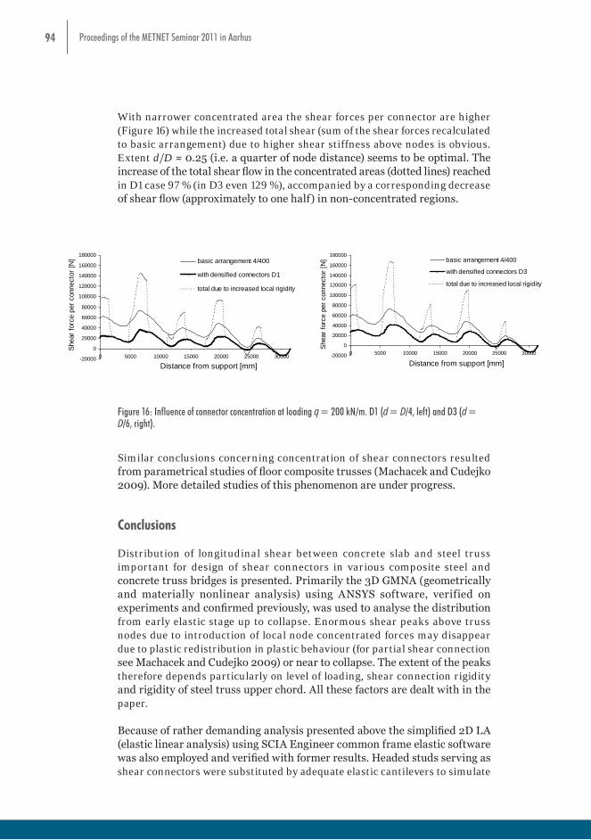
94 Proceedings of the METNET Seminar 2011 in Aarhus
With narrower concentrated area the shear forces per connector are higher (Figure 16) while the increased total shear (sum of the shear forces recalculated to basic arrangement) due to higher shear stiffness above nodes is obvious. Extent d/D ≈ 0.25 (i.e. a quarter of node distance) seems to be optimal. The increase of the total shear flow in the concentrated areas (dotted lines) reached in D1 case 97 % (in D3 even 129 %), accompanied by a corresponding decrease of shear flow (approximately to one half) in non-concentrated regions.
-20000
0
20000
40000
60000
80000
100000
120000
140000
160000
180000
0 5000 10000 15000 20000 25000 30000
Distance from support [mm]
Shea
r for
ce p
er c
onne
ctor
[N] basic arrangement 4/400
with densified connectors D1
total due to increased local rigidity
-20000
0
20000
40000
60000
80000
100000
120000
140000
160000
180000
0 5000 10000 15000 20000 25000 30000
Distance from support [mm]
Shea
r for
ce p
er c
onne
ctor
[N] basic arrangement 4/400
with densified connectors D3
total due to increased local rigidity
Figure 16: Influence of connector concentration at loading q = 200 kN/m.
D1 (d = D/4, left) and D3 (d = D/6, right). Similar conclusions concerning concentration of shear connectors resulted from parametrical studies of floor composite trusses (Machacek and Cudejko 2009). More detailed studies of this phenomenon are under progress. Conclusions Distribution of longitudinal shear between concrete slab and steel truss important for design of shear connectors in various composite steel and concrete truss bridges is presented. Primarily the 3D GMNA (geometrically and materially nonlinear analysis) using ANSYS software, verified on experiments and confirmed previously, was used to analyse the distribution from early elastic stage up to collapse. Enormous shear peaks above truss nodes due to introduction of local node concentrated forces may disappear due to plastic redistribution in plastic behaviour (for partial shear connection see Machacek and Cudejko 2009) or near to collapse. The extent of the peaks therefore depends particularly on level of loading, shear connection rigidity and rigidity of steel truss upper chord. All these factors are dealt with in the paper. Because of rather demanding analysis presented above the simplified 2D LA (elastic linear analysis) using SCIA Engineer common frame elastic software was also employed and verified with former results. Headed studs serving as shear connectors were substituted by adequate elastic cantilevers to simulate their load-slip diagram. Even in spite of other simplification (omission of tension zone in concrete slab) the analysis of longitudinal shear gave reasonable results in fully elastic behaviour provided the appropriate shear stiffness from load-slip diagram was used. Considering initial connector stiffness may lead to slightly exaggerated values of peaks of shear flow above truss nodes. Nevertheless, results of the 2D analysis justify its use in both design practice and future parametrical studies concerning longitudinal shear distribution in composite bridges. Another important question dealt with in the paper concerned the use of Eurocode 4 (EN 1994-2) approach about local effect of concentrated longitudinal shear. It was proved that introduction of truss node forces (see ENV 1994-2 for more detail) and use of Eurocode distribution of longitudinal shear gives reasonable solution even in case of composite trusses. However, the approach depends substantially on effective slab width and the real available ones results into overly conservative results. Likewise shear connector and steel flange rigidities influence considerably the magnitude of shear flow peaks above truss nodes in elastic region, which are not covered by the Standard approach.
Figure 16: Influence of connector concentration at loading q = 200 kN/m. D1 (d = D/4, left) and D3 (d = D/6, right).
Similar conclusions concerning concentration of shear connectors resulted from parametrical studies of floor composite trusses (Machacek and Cudejko 2009). More detailed studies of this phenomenon are under progress.
Conclusions
Distribution of longitudinal shear between concrete slab and steel truss important for design of shear connectors in various composite steel and concrete truss bridges is presented. Primarily the 3D GMNA (geometrically and materially nonlinear analysis) using ANSYS software, verified on experiments and confirmed previously, was used to analyse the distribution from early elastic stage up to collapse. Enormous shear peaks above truss nodes due to introduction of local node concentrated forces may disappear due to plastic redistribution in plastic behaviour (for partial shear connection see Machacek and Cudejko 2009) or near to collapse. The extent of the peaks therefore depends particularly on level of loading, shear connection rigidity and rigidity of steel truss upper chord. All these factors are dealt with in the paper.
Because of rather demanding analysis presented above the simplified 2D LA (elastic linear analysis) using SCIA Engineer common frame elastic software was also employed and verified with former results. Headed studs serving as shear connectors were substituted by adequate elastic cantilevers to simulate

95Proceedings of the METNET Seminar 2011 in Aarhus
their load-slip diagram. Even in spite of other simplification (omission of tension zone in concrete slab) the analysis of longitudinal shear gave reasonable results in fully elastic behaviour provided the appropriate shear stiffness from load-slip diagram was used. Considering initial connector stiffness may lead to slightly exaggerated values of peaks of shear flow above truss nodes. Nevertheless, results of the 2D analysis justify its use in both design practice and future parametrical studies concerning longitudinal shear distribution in composite bridges.
Another important question dealt with in the paper concerned the use of Eurocode 4 (EN 1994-2) approach about local effect of concentrated longitudinal shear. It was proved that introduction of truss node forces (see ENV 1994-2 for more detail) and use of Eurocode distribution of longitudinal shear gives reasonable solution even in case of composite trusses. However, the approach depends substantially on effective slab width and the real available ones results into overly conservative results. Likewise shear connector and steel flange rigidities influence considerably the magnitude of shear flow peaks above truss nodes in elastic region, which are not covered by the Standard approach.
Finally the paper touched upon concentration of shear connectors above truss nodes to cover the shear peaks which is usual in design practice. The concentration necessary for successful design of shear connection however produces considerable redistribution of the shear flow and attracts the flow to concentrated (more rigid) areas. Responsible design in this case therefore requires iterative approach to find optimum value of concentration of shear connectors (both density of connectors and length of concentration) and also rigidity of upper steel flange of the trusses.
Acknowledgement
The support of the Czech Ministry of Education grant MSM 6840770001 is gratefully acknowledged.
References
Brattland, A. - Kennedy, D.J.L. (1992): Flexural test of two full-scale composite trusses. Canadian Journal of Civil Engineering, Vol. 19, pp. 279-295.
Fink, J. (1997): Truss composite bridges. Proc. Conf. Composite Construction-Conventional and Innovative, Innsbruck, pp. 507-512.
Galambos, T.V. - Tide, R.H. (1970): Composite open-web steel joists. Eng. Journal, AISC, pp. 27-36.
96 Proceedings of the METNET Seminar 2011 in Aarhus
Iyengar, S.H. - Zils, J.J. (1973): Composite floor system for Sears Tower. Eng. Journal, Vol. 10, No. 3, pp. 74-81.
Johnson, R.P. (1997): Shear connection for composite bridges and Eurocode 4: Part 2. Proc. Conf. Composite Construction - Conventional and Innovative, Innsbruck, pp. 573-578.
Johnson, R.P. - Ivanov, R.I. (2001): Local effects of concentrated longitudinal shear in composite bridge beams. The Structural Engineer, Vol. 79, No. 5, pp. 19-23.
Machacek, J. - Cudejko, M. (2009): Longitudinal shear in composite steel and concrete trusses. Eng. Structures, Vol. 31, No. 6, pp. 1313-1320.
Machacek, J. - Studnicka, J. (2002): Perforated shear connectors. Steel and Composite Structures, Vol. 2, No. 1, pp. 51-66.
Marcinkowski, Z. – Berkowski, P. (1997): Experimental verification of bearing capacity of composite truss girders. Proc. Conf. Composite Construction - Conventional and Innovative, Innsbruck, pp. 289-294.
Oehlers, D.J. - Coughlan, C.G. (1986): The shear stiffness of stud shear connections in composite beams. J. Construct. Steel Research, No. 6, pp. 273-284.
Skidmore - Owings – Merrill (1992): Design of composite trusses. Publication 83, SCI, Ascot.
Viest, I.M. et al. (1997): Composite construction design for buildings. McGraw-Hill, New York.

97Proceedings of the METNET Seminar 2011 in Aarhus
BEHAVIOUR OF METAL FOAM SANDWICH PANELS
Hayder H. Alkhudery*
Kuldeep S. Virdi**
*College of Engineering, Basrah University, Iraq
**Aarhus School of Engineering, Aarhus University
Abstract
Sandwich panels as used in structures comprise of a foam core enclosed by thin high strength steel faces. This paper discusses currently design formulae of local buckling behaviour of such panels using the finite element method. Multiple wave finite element models were adopted to investigate and examine the adequacy of currently used approach for the design of sandwich panels. The paper presents brief details of the finite element model used including geometry, load pattern and boundary conditions. The selected model gives good agreement with experimental results from Pokharel and Mahendran (2003). The study shows that currently available design formulae are conservative for stocky sandwich plate elements while being over-conservative for high slenderness. A unified design formula of local buckling behaviour applicable to the full range of slenderness is developed.
Introduction
Sandwich panels typically use two different materials to achieve high ultimate strength. As the name implies, a foam core of a very light material is placed between a pair of metal sheets of small thickness. The resulting high bending stiffness coupled with light weight and very good thermal and damping properties make sandwich panels attractive structures for designers. Cost savings are reflected in ease of transport and assembly in all conditions.
Because sandwich panels have flexible less stiff cores, their behaviour is more complex than that for plain plates. Sandwich panels display numerous failure modes which are related to external loads, overall buckling, local buckling, and wrinkling of the external faces. Few guidelines are available for the design and testing of such panels. One important source of information is the European Recommendations for Sandwich Panels (2000) which summarised the state of the art at the time of its publication.
Currently used design formulae of sandwich panels have been suggested by many researchers and are based on assumptions which sometimes do not represent actual structural behaviour of sandwich panels. Most of these formulae are complicated and follow complicated procedure to determine the ultimate strength of panels.

98 Proceedings of the METNET Seminar 2011 in Aarhus
Literature review
Davies and Hakmi (1990, 1991) studied the local buckling behaviour of compressed plate elements supported by relatively weak isotropic core medium, treated as half space linear elastic foundation. This led to a formula for the buckling coefficient of sandwich pane which was used to estimate the ultimate strength of plate using the effective width concept. The authors, however, found that their results did not consistently agree with the experimental results. Improved correlation was obtained by arbitrarily reducing the value of an intermediate parameter. Davies (1993) also introduced design formulae for different types of sandwich panel (profiled/flat) with strength reduction factors based on tests results.
Mahendran and Jeevaharan (1999) carried out laboratory experiments and finite element analysis on steel plate elements of varying yield stresses and thickness with and without supported polystyrene foam core. After validating their finite element analysis using experimental results, they introduced a modified design stress buckling formula. Subsequently, Mahendran and McAndrew (1999 and 2001) studied wrinkling failure of sandwich panels of flat steel faces. They showed, from numerical analysis, that a foam thickness of 75mm or more did not affect the wrinkling stress of the metal face of sandwich panels. Mahendran and McAndrew (2003) extended the above work to study the effects of lightly profiled faces and transverse joints on the flexural wrinkling stress.
Pokharel and Mahendran (2002, 2003, 2004, and 2005) carried out extensive tests on simply supported steel plate element supported by foam core subjected to uniaxial load with two different steel grades and different plate dimension to cover a large range of slenderness ratio. They indicated good agreement between finite element analysis using full-length and half-length models with test results. It should be noted that the papers give different numerical results for the same plate element. The experimental programme of Pokharel and Mahendran (2003) has been adopted as a source of experimental data in this paper.
It is worth pointing out that the authors were unable to find published test results for sandwich panels with full cross-section, that is, both faces and the core included.
Linear elastic buckling
Davies and Hakmi (1990) adopted the critical stress formula of plates with
n as the number buckling half-waves, and included the contribution from the core material.

99Proceedings of the METNET Seminar 2011 in Aarhus
Davies and Hakmi (1990, 1991)studied the local buckling behaviour of compressed plate elements supported by relatively weak isotropic core medium, treated as half space linear elastic foundation. This led to a formula for the buckling coefficient of sandwich pane which was used to estimate the ultimate strength of plate using the effective width concept. The authors, however, found that their results didnot consistently agree with the experimental results. Improved correlation was obtained by arbitrarily reducing the value of an intermediate parameter.Davies (1993) also introduced design formulae for different types of sandwich panel (profiled/flat) with strength reduction factorsbased on tests results. Mahendran and Jeevaharan (1999) carried out laboratory experiments and finite element analysis on steel plate elements of varying yield stresses and thickness with and without supported polystyrene foam core. After validating their finite element analysis using experimental results, they introduced a modified design stress buckling formula. Subsequently, Mahendran and McAndrew (1999 and 2001)studied wrinkling failure of sandwich panels of flat steel faces. They showed, from numerical analysis, that a foam thickness of 75mm or more did not affect the wrinkling stress of the metal face of sandwich panels.Mahendran and McAndrew (2003) extended the above work to study the effects of lightly profiled faces and transverse joints on the flexural wrinkling stress. Pokharel and Mahendran (2003, 2004, 2005) carried out extensive tests on simply supported steel plate element supported by foam core subjected to uniaxial load with two different steel grades and different plate dimension to cover a large range of slenderness ratio. They indicated good agreement between finite element analysis using full-length and half-length models with test results. It should be noted that the papers give different numerical results for the same plate element. The experimental programme of Pokharel and Mahendran (2003) has been adopted as a source of experimental data in this paper. It is worth pointing out that the authors were unable to find published test results for sandwich panels with full cross-section, that is, both faces and the core included.
Linear elastic buckling Davies and Hakmi(1990) adopted the critical stress formula of plates with nas the number buckling half-waves, and included the contribution from the core material.
22
2
)/)(1(12 ff
fcrt tb
EK
(1)
222
2 11
nRnK
(2)
2
2
2
)43)(1()1)(1(24
ffcc
ccf
tb
EE
R
(3)
where:
fE and cE are the Modulus of elasticity of the plate and that of the core, respectively,
cG is the Shear Modulus the core,
f and c are the Poisson ratio of the plate and that of the core, respectively,
where:
fE and cE are the Modulus of elasticity of the plate and that of the core, respectively,
cG is the Shear Modulus the core,
fν and cν are the Poisson ratio of the plate and that of the core, respectively,
b and ft are the width and the thickness, respectively, of the plate,
K is the buckling coefficient,
R is a dimensionless stiffness parameter and,
φ is the ratio of half-wave buckle length a to the width of the plate b
band ft are the width and the thickness, respectively, of the plate, K is the buckling coefficient, R is a dimensionless stiffness parameter and, is the ratio of half-wave buckle length a to the width of the plate b The lowest critical stress relates to the minimum value of buckling coefficient K with respect to .This results in:
012)12(22
22
22
24
nnRn (4)
This equation can be solved for using a suitable numerical method and, hence, K can be evaluated. However, this theoretical method of determining the buckling coefficient K has not been adopted in the design procedures because it is seen as complicated. For practical applications, an explicit mathematical formula is preferred. Various formulae have been proposed in literature, for example, Hassinen proposed in Davies, Hakmi and Hassinen (1991):
2703.0415.04 RK with 3/1
f
c
f EE
tbR (5)
Finite element model The finite element program used to investigate local buckling and ultimate strength behaviour of sandwich panels in this study is MARC 2010 with PATRAN 2010 as pre-and post-processor. The steel face plate was modelled using four-node quadrilateral shell elements (CQUAD4) and the foam core was meshed with eight-node solid brick elements (CHEXA). In order to reduce processing time, in this work, a half-length model together with half width across and with appropriate boundary conditions using symmetry, has been used. For elastic buckling of plates, it is customary to consider the elastic buckling behaviour of square plates, since the theoretical critical load of plates of aspect ratio 1, 2, 3, etc remains unchanged. In order to check the validity of using an approximately square when considering elastic and inelastic buckling of sandwich plates, comparisons have also been made with another reduced model used based on multiple half waves (2.5a×0.5b ) representing 5 half waves as shown in Figure 1 as well as (1.5a×0.5b ) representing 3 half waves and a single half wave (0.5a×0.5b ) along the length of the specimen.
The lowest critical stress relates to the minimum value of buckling coefficient K with respect toφ .This results in:
band ft are the width and the thickness, respectively, of the plate, K is the buckling coefficient, R is a dimensionless stiffness parameter and, is the ratio of half-wave buckle length a to the width of the plate b The lowest critical stress relates to the minimum value of buckling coefficient K with respect to .This results in:
012)12(22
22
22
24
nnRn (4)
This equation can be solved for using a suitable numerical method and, hence, K can be evaluated. However, this theoretical method of determining the buckling coefficient K has not been adopted in the design procedures because it is seen as complicated. For practical applications, an explicit mathematical formula is preferred. Various formulae have been proposed in literature, for example, Hassinen proposed in Davies, Hakmi and Hassinen (1991):
2703.0415.04 RK with 3/1
f
c
f EE
tbR (5)
Finite element model The finite element program used to investigate local buckling and ultimate strength behaviour of sandwich panels in this study is MARC 2010 with PATRAN 2010 as pre-and post-processor. The steel face plate was modelled using four-node quadrilateral shell elements (CQUAD4) and the foam core was meshed with eight-node solid brick elements (CHEXA). In order to reduce processing time, in this work, a half-length model together with half width across and with appropriate boundary conditions using symmetry, has been used. For elastic buckling of plates, it is customary to consider the elastic buckling behaviour of square plates, since the theoretical critical load of plates of aspect ratio 1, 2, 3, etc remains unchanged. In order to check the validity of using an approximately square when considering elastic and inelastic buckling of sandwich plates, comparisons have also been made with another reduced model used based on multiple half waves (2.5a×0.5b ) representing 5 half waves as shown in Figure 1 as well as (1.5a×0.5b ) representing 3 half waves and a single half wave (0.5a×0.5b ) along the length of the specimen.
This equation can be solved for φ using a suitable numerical method and, hence, K can be evaluated. However, this theoretical method of determining the buckling coefficient K has not been adopted in the design procedures because it is seen as complicated.

100 Proceedings of the METNET Seminar 2011 in Aarhus
For practical applications, an explicit mathematical formula is preferred. Various formulae have been proposed in literature, for example, Hassinen proposed in Davies, Hakmi and Hassinen (1991):
Finite element model
The finite element program used to investigate local buckling and ultimate strength behaviour of sandwich panels in this study is MARC 2010 with PATRAN 2010 as pre-and post-processor. The steel face plate was modelled using four-node quadrilateral shell elements (CQUAD4) and the foam core was meshed with eight-node solid brick elements (CHEXA). In order to reduce processing time, in this work, a half-length model together with half width across and with appropriate boundary conditions using symmetry, has been used.
For elastic buckling of plates, it is customary to consider the elastic buckling behaviour of square plates, since the theoretical critical load of plates of aspect ratio 1, 2, 3, etc remains unchanged. In order to check the validity of using an approximately square when considering elastic and inelastic buckling of sandwich plates, comparisons have also been made with another reduced model used based on multiple half waves (2.5 a ×0.5 b ) representing 5 half waves as shown in Figure 1 as well as (1.5 a ×0.5 b ) representing 3 half waves and a single half wave (0.5 a ×0.5 b ) along the length of the specimen.
2.5a
bb/2
pp
x
yz
a a a a a
Core
Metal face
Figure 1 -Five half waves buckling model
Geometric imperfections The presence of geometric imperfections seriously affects the strength of compressed plate elements and ignoring them in the numerical analysis could result in unrealistic strength predictions. It is generally accepted that the most detrimental type of imperfection is one which has the same shape as the critical local buckling mode. In practice, the maximum imperfection magnitudes are specified in terms of either the thickness or the width of the plates. Experimental observations show that the actual magnitudes of geometric imperfections in sandwich panels are quite small. The maximum imperfection adopted in this paper is 0.1tfas adopted by Pokharel and Mahendran (2004), where tf. Is the thickness of the metal sheet. Numerical convergence study As the mesh density increases, the accuracy of a finite element model also generally increases and converges to a numerically ‘correct’ solution. A convergence study was conducted with gradually decreasing mesh sizes for the half-length model. It was found that a mesh with 10mm×10mm square surface shell elements (for steel plate) and 10mm×10mm×5mm solid elements (foam depth) provided satisfactory results in terms of accuracy, both for elastic and inelastic analyses. Comparison of finite element analysis and experimental results To calibrate the finite element calculations all 50 specimens tested by Pokharel and Mahendran (2004) were analysed using the half-length model. For geometric and material data, reference should be made to the original source. As first step, linear elastic buckling analysis was carried out to evaluate the buckling shape which was then used to impose an imperfection shape with(0.1tf) as the maximum imperfection for the inelastic analysis. Table 1 presents the comparison of finite element ultimate stress and experimental ultimate strength. For reasons of space, only selected cases are shown, but the study covered the full range of slenderness. The mean values of the ratio of finite element and experimental failure loads were 0.84 and 0.91 for G550 and G250, respectively. The corresponding coefficients of variation (COV) were 0.07 and 0.08.
Table 1 - Comparison of FEA Results with Experimental Results Test Grade 550 Steel Grade 250 Steel
Figure 1 -Five half waves buckling model
Geometric imperfections
The presence of geometric imperfections seriously affects the strength of compressed plate elements and ignoring them in the numerical analysis could result in unrealistic strength predictions. It is generally accepted that the most detrimental type of imperfection is one which has the same shape as the critical local buckling mode. In practice, the maximum imperfection magnitudes are specified in terms of either the thickness or the width of
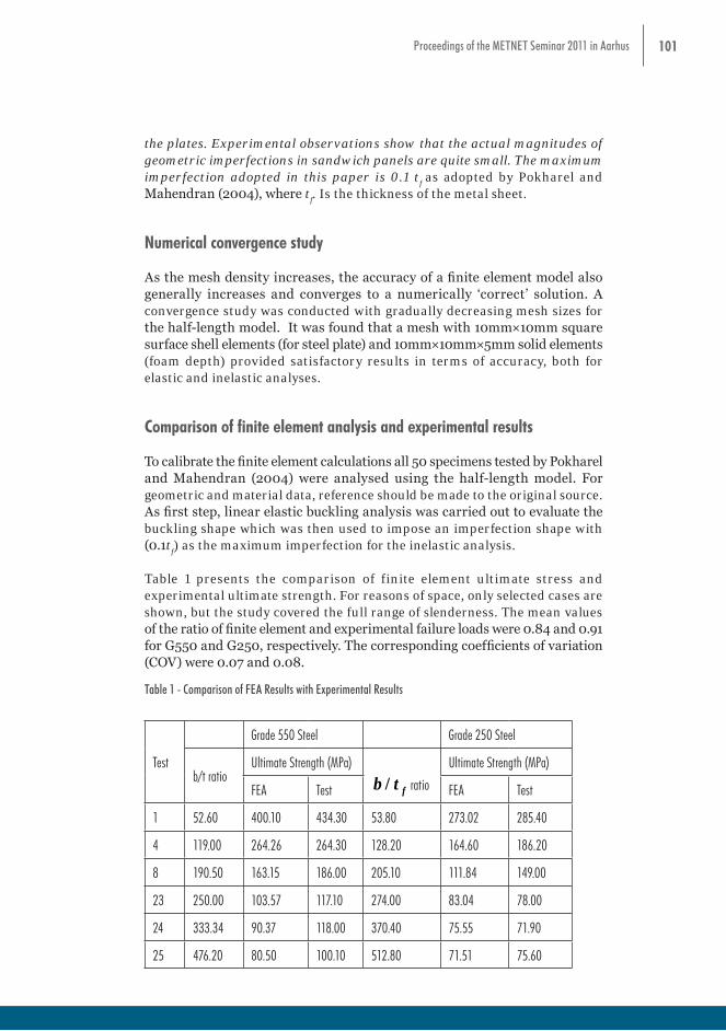
101Proceedings of the METNET Seminar 2011 in Aarhus
the plates. Experimental observations show that the actual magnitudes of geometric imperfections in sandwich panels are quite small. The maximum imperfection adopted in this paper is 0.1 t
f as adopted by Pokharel and
Mahendran (2004), where tf. Is the thickness of the metal sheet.
Numerical convergence study
As the mesh density increases, the accuracy of a finite element model also generally increases and converges to a numerically ‘correct’ solution. A convergence study was conducted with gradually decreasing mesh sizes for the half-length model. It was found that a mesh with 10mm×10mm square surface shell elements (for steel plate) and 10mm×10mm×5mm solid elements (foam depth) provided satisfactory results in terms of accuracy, both for elastic and inelastic analyses.
Comparison of finite element analysis and experimental results
To calibrate the finite element calculations all 50 specimens tested by Pokharel and Mahendran (2004) were analysed using the half-length model. For geometric and material data, reference should be made to the original source. As first step, linear elastic buckling analysis was carried out to evaluate the buckling shape which was then used to impose an imperfection shape with (0.1t
f) as the maximum imperfection for the inelastic analysis.
Table 1 presents the comparison of finite element ultimate stress and experimental ultimate strength. For reasons of space, only selected cases are shown, but the study covered the full range of slenderness. The mean values of the ratio of finite element and experimental failure loads were 0.84 and 0.91 for G550 and G250, respectively. The corresponding coefficients of variation (COV) were 0.07 and 0.08.
Table 1 - Comparison of FEA Results with Experimental Results
Test
Grade 550 Steel Grade 250 Steel
b/t ratioUltimate Strength (MPa)
ftb / ratio
Ultimate Strength (MPa)
FEA Test FEA Test
1 52.60 400.10 434.30 53.80 273.02 285.40
4 119.00 264.26 264.30 128.20 164.60 186.20
8 190.50 163.15 186.00 205.10 111.84 149.00
23 250.00 103.57 117.10 274.00 83.04 78.00
24 333.34 90.37 118.00 370.40 75.55 71.90
25 476.20 80.50 100.10 512.80 71.51 75.60
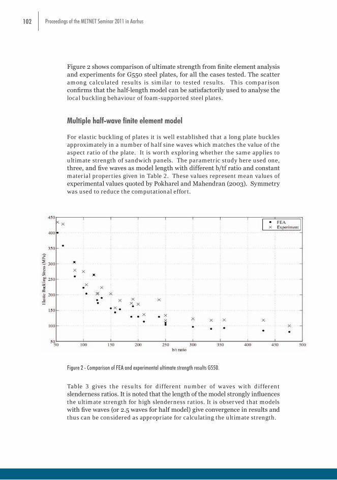
102 Proceedings of the METNET Seminar 2011 in Aarhus
Figure 2 shows comparison of ultimate strength from finite element analysis and experiments for G550 steel plates, for all the cases tested. The scatter among calculated results is similar to tested results. This comparison confirms that the half-length model can be satisfactorily used to analyse the local buckling behaviour of foam-supported steel plates.
Multiple half-wave finite element model
For elastic buckling of plates it is well established that a long plate buckles approximately in a number of half sine waves which matches the value of the aspect ratio of the plate. It is worth exploring whether the same applies to ultimate strength of sandwich panels. The parametric study here used one, three, and five waves as model length with different b/tf ratio and constant material properties given in Table 2. These values represent mean values of experimental values quoted by Pokharel and Mahendran (2003). Symmetry was used to reduce the computational effort.
b/t ratio Ultimate Strength
(MPa) ftb / ratioUltimate Strength
(MPa) FEA Test FEA Test
1 52.60 400.10 434.30 53.80 273.02 285.40 4 119.00 264.26 264.30 128.20 164.60 186.20 8 190.50 163.15 186.00 205.10 111.84 149.00
23 250.00 103.57 117.10 274.00 83.04 78.00 24 333.34 90.37 118.00 370.40 75.55 71.90 25 476.20 80.50 100.10 512.80 71.51 75.60
Figure 2 shows comparison of ultimate strength from finite element analysis and experiments for G550 steel plates, for all the cases tested. The scatter among calculated results is similar to tested results. This comparison confirms that the half-length model can be satisfactorily used to analyse the local buckling behaviour of foam-supported steel plates. Multiple half-wave finite element model For elastic buckling of plates it is well established that a long plate buckles approximately in a number of half sine waves which matches the value of the aspect ratio of the plate. It is worth exploring whether the same applies to ultimate strength of sandwich panels. The parametric study here used one, three, and five waves as model length with different b/t ratio and constant material properties given in Table 2. These values represent mean values of experimental values quoted by Pokharel and Mahendran (2003). Symmetry was used to reduce the computational effort.
Figure 2 - Comparison of FEA and experimental ultimate strength results G550.
Table 3 gives the results for different number of waves with different slenderness ratios. It is noted that the length of the model strongly influences the ultimate strength for high slenderness ratios. It is observed that models with five waves (or 2.5 waves for half model) give convergence in results and thus can be considered as appropriate for calculating the ultimate strength.

103Proceedings of the METNET Seminar 2011 in Aarhus
Table 2 - Material properties of faces and core for multiple half-waves mode
MaterialYoung Modulus E
(MPa)Poisson’s ratio ν
Shear Modulus
(MPa)Ultimate strength(MPa)
Steel face 233000.00 0.30 89615.38 675.00
Foam core 3.80 0.08 1.76 -
Table 3 - Variation of ultimate strength with number of half waves
b/t ratioBuckling stress (MPa) Ultimate strength (MPa)
1 wave 3waves 5waves 7waves 1 wave 3waves 5waves 7waves
63 271.71 272.48 272.57 272.65 345.91 345.40 346.55 345.93
125 134.09 134.63 134.80 134.41 201.712 203.55 203.46 203.35
200 109.06 109.64 109.81 109.91 136.34 144.31 144.23 144.19
250 103.54 104.23 104.26 104.36 120.99 129.80 129.35 129.74
500 96.63 96.89 96.97 97.03 96.80 103.54 104.47 104.67
Assumption of core acting as elastic foundation
Davies and Hakmi (1990) postulated that to simulate the behaviour of the sandwich panel, it was sufficient to consider a single plate and treat the foam core as an elastic foundation. To investigate validity of this principle, a parametric study was carried out for different plate slenderness ratios with the full cross-section of two faces together with foam core. Figure 3 shows the typical buckled shape of the 5 half-wave model (symmetrical one-quarter). The near absence of deformations towards the bottom of the core confirms the conclusion drawn earlier that the very soft core eliminates buckling of one plate influencing the behaviour of the plate at the other face.
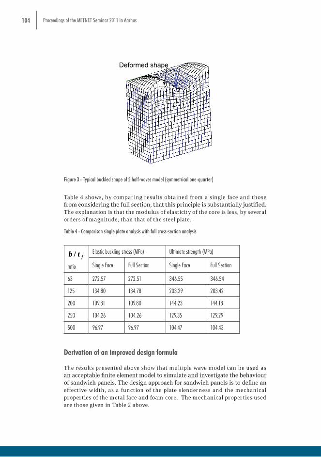
104 Proceedings of the METNET Seminar 2011 in Aarhus
Table 2 - Material properties of faces and core for multiple half-waves model
Material Young
Modulus E (MPa)
Poisson’s ratio
Shear Modulus (MPa)
Ultimate strength(MPa)
Steel face 233000.00 0.30 89615.38 675.00Foam core 3.80 0.08 1.76 -
Table 3 - Variation of ultimate strength with number of half waves b/t
ratio Buckling stress (MPa) Ultimate strength (MPa)
1 wave 3waves 5waves 7waves 1 wave 3waves 5waves 7waves63 271.71 272.48 272.57 272.65 345.91 345.40 346.55 345.93
125 134.09 134.63 134.80 134.41 201.712 203.55 203.46 203.35200 109.06 109.64 109.81 109.91 136.34 144.31 144.23 144.19250 103.54 104.23 104.26 104.36 120.99 129.80 129.35 129.74500 96.63 96.89 96.97 97.03 96.80 103.54 104.47 104.67
Assumption of core acting as elastic foundation Davies and Hakmi (1990) postulated that to simulate the behaviour of the sandwich panel, it was sufficient to consider a single plate and treat the foam core as an elastic foundation. To investigate validity of this principle, a parametric study was carried out for different plate slenderness ratios with the full cross-section of two faces together with foam core. Figure 3 shows the typical buckled shape of the 5 half-wave model (symmetrical one-quarter). The near absence of deformations towards the bottom of the core confirms the conclusion drawn earlier that the very soft core eliminates buckling of one plate influencing the behaviour of the plate at the other face.
Figure 3 - Typical buckled shape of 5 half-waves model (symmetrical one-quarter)
Table 4 shows, by comparing results obtained from a single face and those from considering the full section, that this principle is substantially justified. The explanation is that the modulus of elasticity of the core is less, by several orders of magnitude, than that of the steel plate.
Table 4 - Comparison single plate analysis with full cross-section analysis
Deformed shape
Figure 3 - Typical buckled shape of 5 half-waves model (symmetrical one-quarter)
Table 4 shows, by comparing results obtained from a single face and those from considering the full section, that this principle is substantially justified. The explanation is that the modulus of elasticity of the core is less, by several orders of magnitude, than that of the steel plate.
Table 4 - Comparison single plate analysis with full cross-section analysis
ftb /
ratio
Elastic buckling stress (MPa) Ultimate strength (MPa)
Single Face Full Section Single Face Full Section
63 272.57 272.51 346.55 346.54
125 134.80 134.78 203.29 203.42
200 109.81 109.80 144.23 144.18
250 104.26 104.26 129.35 129.29
500 96.97 96.97 104.47 104.43
Derivation of an improved design formula
The results presented above show that multiple wave model can be used as an acceptable finite element model to simulate and investigate the behaviour of sandwich panels. The design approach for sandwich panels is to define an effective width, as a function of the plate slenderness and the mechanical properties of the metal face and foam core. The mechanical properties used are those given in Table 2 above.

105Proceedings of the METNET Seminar 2011 in Aarhus
As in the case of the assessing the performance of half wave-length model, this study also first carries out an elastic buckling (eigen value) analysis. The buckled shape with the lowest critical load is then used to define the shape of imperfections with amplitude of ft1.0 , followed by non-linear ultimate strength analysis. Table 5 gives the wave length and the critical buckling stress obtained from the finite element method
The simple approach adopted in design recommendations is to use an effective width which can be assumed to develop the yield stress. Thus:
ftb / ratio
Elastic buckling stress (MPa)
Ultimate strength (MPa)
Single Face
Full Section
Single Face
Full Section
63 272.57 272.51 346.55 346.54 125 134.80 134.78 203.29 203.42 200 109.81 109.80 144.23 144.18 250 104.26 104.26 129.35 129.29 500 96.97 96.97 104.47 104.43
Derivation of an improved design formula The results presented above show that multiple wave model can be used as an acceptable finite element model to simulate and investigate the behaviour of sandwich panels. The design approach for sandwich panels is to define an effective width, as a function of the plate slenderness and the mechanical properties of the metal face and foam core. The mechanical properties used are those given in Table 2 above. As in the case of the assessing the performance of half wave-length model, this study also first carries out an elastic buckling (eigen value) analysis. The buckled shape with the lowest critical load is then used to define the shape of imperfections with an amplitude of ft1.0 , followed by non-linear ultimate strength analysis. Table 5 gives the wave lengthand the critical buckling stress obtained from the finite element method The simple approach adopted in design recommendations is to use an effective width which can be assumed to develop the yield stress. Thus:
stressYieldstrengthUltimate
bbeff (6)
The effective width ratios so obtained from the nonlinear finite element analysis are compared with several other approaches available in literature:
(1) using the K values suggested by Davies and Hakmi (1990), (2) ECCS(2000) (3) Two formulae suggested by Pokharel and Mahendran (2002 and 2005)
These are plotted in Figure 4.
Table 5 ‚ Results of ultimate strength of sandwich panels with steel Grade 550.
No. b (mm)
ft (mm)
ftb /ratio
Wave length (mm)
2/L (mm)
Critical stress (MPa)
Ultimate strength (MPa)
1 50 0.8 63 42.4 106 272.57 346.55 2 50 0.7 71 40.0 100 227.65 309.75 3 50 0.6 83 36.8 92 189.82 273.76 4 50 0.5 100 32.8 82 159.00 238.42 5 50 0.4 125 28.4 71 134.80 203.29
The effective width ratios so obtained from the nonlinear finite element analysis are compared with several other approaches available in literature:
(a) using the K values suggested by Davies and Hakmi (1990),
(b) ECCS(2000)
(c) Two formulae suggested by Pokharel and Mahendran (2002 and 2005)
These are plotted in Figure 4.
Table 5 ‚ Results of ultimate strength of sandwich panels with steel Grade 550.
No. b (mm)ft
(mm)
ftb /ratio
Wave length
(mm)2/L
(mm)
Critical stress
(MPa)Ultimate strength (MPa)
1 50 0.8 63 42.4 106 272.57 346.55
2 50 0.7 71 40.0 100 227.65 309.75
3 50 0.6 83 36.8 92 189.82 273.76
4 50 0.5 100 32.8 82 159.00 238.42
5 50 0.4 125 28.4 71 134.80 203.29
6 100 0.7 143 50.8 127 125.09 177.26
7 100 0.6 167 44.8 112 116.74 160.21
8 100 0.5 200 38.4 96 109.81 144.23
9 150 0.7 214 54.4 136 107.79 137.61
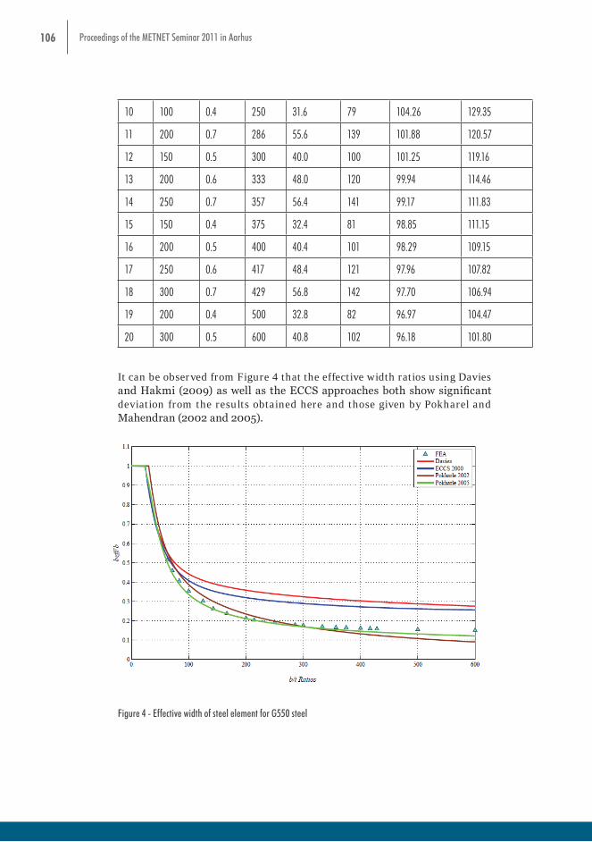
106 Proceedings of the METNET Seminar 2011 in Aarhus
10 100 0.4 250 31.6 79 104.26 129.35
11 200 0.7 286 55.6 139 101.88 120.57
12 150 0.5 300 40.0 100 101.25 119.16
13 200 0.6 333 48.0 120 99.94 114.46
14 250 0.7 357 56.4 141 99.17 111.83
15 150 0.4 375 32.4 81 98.85 111.15
16 200 0.5 400 40.4 101 98.29 109.15
17 250 0.6 417 48.4 121 97.96 107.82
18 300 0.7 429 56.8 142 97.70 106.94
19 200 0.4 500 32.8 82 96.97 104.47
20 300 0.5 600 40.8 102 96.18 101.80
It can be observed from Figure 4 that the effective width ratios using Davies and Hakmi (2009) as well as the ECCS approaches both show significant deviation from the results obtained here and those given by Pokharel and Mahendran (2002 and 2005).
6 100 0.7 143 50.8 127 125.09 177.26 7 100 0.6 167 44.8 112 116.74 160.21 8 100 0.5 200 38.4 96 109.81 144.23 9 150 0.7 214 54.4 136 107.79 137.61
10 100 0.4 250 31.6 79 104.26 129.35 11 200 0.7 286 55.6 139 101.88 120.57 12 150 0.5 300 40.0 100 101.25 119.16 13 200 0.6 333 48.0 120 99.94 114.46 14 250 0.7 357 56.4 141 99.17 111.83 15 150 0.4 375 32.4 81 98.85 111.15 16 200 0.5 400 40.4 101 98.29 109.15 17 250 0.6 417 48.4 121 97.96 107.82 18 300 0.7 429 56.8 142 97.70 106.94 19 200 0.4 500 32.8 82 96.97 104.47 20 300 0.5 600 40.8 102 96.18 101.80
It can be observed from Figure 4 that the effective width ratios using Davies and Hakmi (2009) as well as the ECCS approaches both show significant deviation from the results obtained here and those given by Pokharel and Mahendran (2002 and 2005).
Figure 4 - Effective width of steel element for G550 steel
Effect of yield stress Previous studies focused on two values of yield stress. To study the wider effect of yield strength of the metal surface, further calculations were carried out and the results are plotted in Figure 5. It will be seen that at lower slenderness ratios, the ultimate strength of sandwich panel ratio is significantly affected by the yield stress of steel face, while the effects become marginal for plates with higher slenderness.
Figure 4 - Effective width of steel element for G550 steel
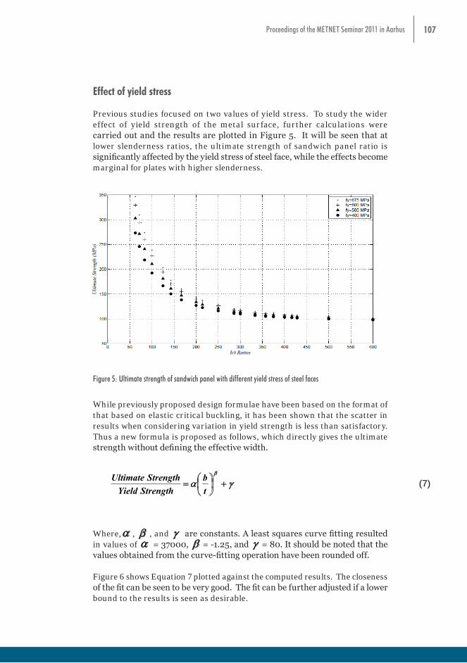
107Proceedings of the METNET Seminar 2011 in Aarhus
Effect of yield stress
Previous studies focused on two values of yield stress. To study the wider effect of yield strength of the metal surface, further calculations were carried out and the results are plotted in Figure 5. It will be seen that at lower slenderness ratios, the ultimate strength of sandwich panel ratio is significantly affected by the yield stress of steel face, while the effects become marginal for plates with higher slenderness.
Figure 5: Ultimate strength of sandwich panel with different yield stress of steel faces
While previously proposed design formulae have been based on the format of that based on elastic critical buckling, it has been shown that the scatter in results when considering variation in yield strength, is less than satisfactory. Thus a new formula is proposed as follows, which directly gives the ultimate strength without defining the effective width.
tb
StrengthYieldStrengthUltimate (7)
Where, , , and are constants. A least squares curve fitting resulted in values of = 70, = 1.25, and = 0.15. It should be noted that the values obtained from the curve-fitting operation have been rounded off. Figure 6 shows Equation 7 plotted against the computed results. The closeness of the fit can be seen to be very good.
Figure 5: Ultimate strength of sandwich panel with different yield stress of steel faces
While previously proposed design formulae have been based on the format of that based on elastic critical buckling, it has been shown that the scatter in results when considering variation in yield strength is less than satisfactory. Thus a new formula is proposed as follows, which directly gives the ultimate strength without defining the effective width.
Figure 5: Ultimate strength of sandwich panel with different yield stress of steel faces
While previously proposed design formulae have been based on the format of that based on elastic critical buckling, it has been shown that the scatter in results when considering variation in yield strength, is less than satisfactory. Thus a new formula is proposed as follows, which directly gives the ultimate strength without defining the effective width.
tb
StrengthYieldStrengthUltimate (7)
Where, , , and are constants. A least squares curve fitting resulted in values of = 70, = 1.25, and = 0.15. It should be noted that the values obtained from the curve-fitting operation have been rounded off. Figure 6 shows Equation 7 plotted against the computed results. The closeness of the fit can be seen to be very good.
Where,a , β , and g are constants. A least squares curve fitting resulted in values of a = 37000, β = -1.25, and g = 80. It should be noted that the values obtained from the curve-fitting operation have been rounded off.
Figure 6 shows Equation 7 plotted against the computed results. The closeness of the fit can be seen to be very good. The fit can be further adjusted if a lower bound to the results is seen as desirable.
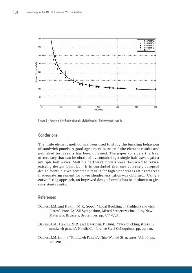
108 Proceedings of the METNET Seminar 2011 in Aarhus
Figure 6 - Formula of ultimate strength plotted against finite element results
Conclusions The finite element method has been used to study the buckling behaviour of sandwich panels. A good agreement between finite element results and published test results has been obtained. The paper considers the level of accuracy that can be obtained by considering a single half wave against multiple half waves. Multiple half wave model was then used to review existing design formulae. It is concluded that one currently accepted design formula gives acceptable results for high slenderness ratios whereas inadequate agreement for lower slenderness ratios was obtained. Using a curve-fitting approach, an improved design formula has been shown to give consistent results. References Davies, J.M. and Hakmi, M.R. (1990), “Local Buckling of Profiled Sandwich Plates”, Proc. IABSE Symposium, Mixed Structures including New Materials, Brussels, September, pp. 533-538. Davies, J.M., Hakmi, M.R. and Hassinen, P. (1991), “Face buckling stress in sandwich panels”, Nordic Conference Steel Colloquium, pp. 99-110. Davies, J.M. (1993), “Sandwich Panels”, Thin-Walled Structures, Vol. 16, pp. 179-198. Davies, J.M. and Heselius, L. (1993), “Design recommendations for sandwich panels”, Journal of Building Research and Information, Vol. 21,No.3, pp.157-161. Hassinen, P. (1997), “Evaluation of the compression strength of profiled metal sheet faces of sandwich panels”, Thin-Walled Structures Vol. 27, No. 1, pp, 31-41.
Figure 6 - Formula of ultimate strength plotted against finite element results
Conclusions
The finite element method has been used to study the buckling behaviour of sandwich panels. A good agreement between finite element results and published test results has been obtained. The paper considers the level of accuracy that can be obtained by considering a single half wave against multiple half waves. Multiple half wave models were then used to review existing design formulae. It is concluded that one currently accepted design formula gives acceptable results for high slenderness ratios whereas inadequate agreement for lower slenderness ratios was obtained. Using a curve-fitting approach, an improved design formula has been shown to give consistent results.
References
Davies, J.M. and Hakmi, M.R. (1990), “Local Buckling of Profiled Sandwich Plates”, Proc. IABSE Symposium, Mixed Structures including New Materials, Brussels, September, pp. 533-538.
Davies, J.M., Hakmi, M.R. and Hassinen, P. (1991), “Face buckling stress in sandwich panels”, Nordic Conference Steel Colloquium, pp. 99-110.
Davies, J.M. (1993), “Sandwich Panels”, Thin-Walled Structures, Vol. 16, pp. 179-198.

109Proceedings of the METNET Seminar 2011 in Aarhus
Davies, J.M. and Heselius, L. (1993), “Design recommendations for sandwich panels”, Journal of Building Research and Information, Vol. 21,No.3, pp.157-161.
Hassinen, P. (1997), “Evaluation of the compression strength of profiled metal sheet faces of sandwich panels”, Thin-Walled Structures Vol. 27, No. 1, pp, 31-41.
Hassinen, P. (1995), “Compression failure modes of thin profiled metal sheet faces of sandwich panels”, Sandwich Construction 3-Proceedings of the Third International Conference, Southampton, pp. 205-214.
International Council for Building Research, Studies and Documentation (CIB) (2000), “European Recommendations for Sandwich Panels Part 1: Design”, CIB Publication.
Mahendran, M. and Jeevaharan, M. (1999), “Local buckling behaviour of steel plate elements supported by a plastic foam material”, Structural Engineering and Mechanics, Vol. 7, No. 5, pp. 433-445.
Mahendran, M. and McAndrew, D. (2001), “Effects of Foam Joints on the Flexural Wrinkling Strength of Sandwich Panels”, Steel Structures, Vol. 1, pp. 105-112.
Mahendran, M. and McAndrew, D, (2003) ’’Flexural Wrinkling Strength of Lightly Profiled Sandwich Panels with Transverse Joints in the Foam Core’’, Advance in structural Engineering 6(4): pp.325-337.
McAndrew, D. and Mahendran, M. (1999) “Flexural Wrinkling Failure of Sandwich Panels with Foam Joints”, Proc. 4th International Conference on Steel and Aluminium Structures, Helsinki, Finland, pp.301-308.
Pokharel, N., and Mahendran, M., (2002), ‘’Numerical Modelling of sandwich panels Subject to local buckling’’, Proc. of the 17th Australasian Conference on the Mechanical of Structures and Materials, Gold Coast, Queensland, Australia.
Pokharel, N, and Mahendran, M. (2003), ‘Experimental investigation and design of sandwich panels subject to local buckling effects’’, Journal of Constructional Steel Research 59 (2003) 1533-1552.
Pokharel, N, and Mahendran, M. (2004),‘’Finite element analysis and design of sandwich panels subject to local buckling effects’’, Thin-Walled Structures, Volume 42, Issue 4, April 2004, Pages 589-611.
Pokharel, N, and Mahendran, M. (2005), “An investigation of lightly profiled sandwich panels subject to local buckling and flexural wrinkling effects’’, Journal of Constructional Steel Research 61 (2005) 984 –1006.

110 Proceedings of the METNET Seminar 2011 in Aarhus
PRODUCT INNOVATION IN SMES: A WEB-BASED SUPPORTING TOOL AND CASE STUDIES
Stelian Brad*Adrian Chioreanu*
Zsolt Nagy**
*Technical University of Cluj-NapocaEngineering Design and Robotics Department
Research Centre in Engineering and Management of Innovation
**Technical University of Cluj-NapocaSteel Department
Abstract
Customized approaches for tackling particular cases of product innovation address technology-oriented SMEs. A web-based supporting tool of product innovation process is introduced in this paper. Case-based roadmaps are generated to lead the innovation project. Domain-specific ontologies are used in this respect. Tools for product planning, innovative problem solving, market and technology search are part of these roadmaps. Priorities of intervention are revealed. Searching time for appropriate solutions is significantly diminished. Orientation towards continuous monitoring of the technological progress in the areas of interest is envisaged and the monitoring mechanism is simplified. Extended remote cooperation between team members in the innovation project is ensured. An exploratory case study from electromechanical field illustrates the value of the software tool. Expanding possibilities of the software platform to other engineering fields (e.g. steel construction) is also highlighted.
Introduction
Rosenbusch et al. (2011) have shown that technical innovation creates value for SMEs, meaning differentiation from competitors, higher cost margins, customer loyalty and technological distance from imitators. Compared to big companies, SMEs have several strengths for setting up technical innovation projects like: rapid response to market changes, cost effective structures, ability to reconfigure in short time existing resources and customer focus attitude (Branzei and Vertinsky 2006). However, access to venture capital and highly skilled human resources to drive mature technical innovation projects is still the challenge of this category of companies (Branzei and Vertinsky 2006).

111Proceedings of the METNET Seminar 2011 in Aarhus
Under such circumstances, intelligent and fast management of knowledge represents a crucial factor that may change new projects outcomes likely as a result of the critical role of new knowledge building, sharing and communication among team members (Solomom 2001). Moreover, Yang et al. (2011) revealed that knowledge management practice adoption supports the transfer of new knowledge to SMEs, while it also helps improve project performance by gaining a greater understanding of the technical innovation process. Bhatt et al. (2010) have demonstrated that SMEs can leverage knowledge to respond to market opportunities, thereby creating competitive advantage. An empirical study done by Fink and Neumann (2007) disclosed the strong relationship between software/IT capabilities of an SME and the overall organizational agility, by pointing out that IT-based intelligent knowledge management systems allow SMEs to respond faster and more effective to the dynamic nature of the market. Despite this, most of SMEs fail in maturely adopting such technologies. One of the barriers here is the lack of skills to handle effectively and to use in an integrated way, in due time, the internal and external available knowledge, data and information.
Depending of their field of activity, SMEs may have lack of information (e.g. the systematic information, which is available, being often fragmentary), or may be bombarded with information often redundant or useless, thus toxic for the technical innovation process. SMEs usually lack the skilled personnel able to deal with the hassle of going through patents, technical documentation, scientific articles, as well as the skilled personnel for tackling specific technical aspects needed to realize the innovative product (Malerba 2007). This is all due to the fact SMEs miss effective activity-oriented support instruments (Yang et al. 2011) that help them access relevant information and offer them the possibility to search, filter and be informed on the latest available data.
To this, reality shows that each technical innovation project is a unique case, which has to be approached by teams composed of different experts (Clemons and Kroth 2010). Furthermore, each technical innovation project follows a different path, thus, no universal innovation roadmap exists that the company may use. Thus, small businesses can only tackle a few technical innovation projects at a time, which makes them difficult to balance the economic risks (Schwarz et al. 2006).
Consequently, for effective technical innovations, traditional SMEs need to use experts from outside the company, which are quite expensive and not necessarily in deep familiar with the business case. Hence, it is the first purpose of this paper to promote the concept of product-service systems (PSS) (Brad 2009; Brad et al. 2010; Kang and Wimmer 2008; Tukker and Tischner 2006), which exploits the power of the mix of marketable software solutions and expert services as a reliable solution for improving the effectiveness of technical innovation within SMEs. The second purpose of the paper is to introduce a novel web-based software platform (called Tech-It-Easy) that supports product innovation projects in a systematic and context-aware way (using ontologies), considering the PSS concept, too. The third purpose of this work is to show how Tech-It-Easy handles real projects. Tech-It-Easy

112 Proceedings of the METNET Seminar 2011 in Aarhus
has been specifically designed to support SMEs from the electromechanical industry. However, the potential for expanding the use of Tech-It-Easy in other industries is very high. Thus, the last purpose of the paper is to highlight this potential in a case study from the metal sector. Time-to-innovation, costs and technical value of the products treated in the case studies are significantly improved.
Positioning of the Tech-It-Easy Software Platform
Novel technologies and new infrastructure capabilities are shaping the behaviour of the production sector (Gunasekaran et al. 2008). Participants (stakeholders) from different business processes, suppliers or producers, experts or researchers, should be able of being involved in the innovation process iteratively, as well as simultaneously, in any number and from any geographical location by means of a collaborative innovation platform (Malerba 2007). In this way the cost of using external experts is diminished. If we are talking about SMEs with low innovation profile (or beginners in innovation), it is desirable having a guideline to the innovation process flow. But, as it was mentioned in the section before, the development of an innovative product is a dynamic and context- dependent process. Therefore, dynamic roadmaps should accompany team members during technical innovation phases. Such innovation roadmaps, beyond being dedicated to the specific field of interest, should be able to evolve and thus to react in real-time to technology, method and market changes. While companies are able to choose among several collaborative meeting, document shearing, videoconference, collaborative work, or innovation software (Clemons and Kroth 2010; Lojeski 2009), no framework that supports SMEs in dealing effectively with the technical innovation process in all of its aspects does exist at this moment.
For example, studies done by Hüsig and Kohn (2009) have shown that nearly half of all product development tools offer some sort of support for idea management, while nearly a third of them offer support also for the product development strategy. Only about a sixth of them are aimed at patent management. Less than half of the companies that undergo a product development activity use a web collaborative software to support their creative work (Hyeongon et al. 2011) and less than a fifth of them use web-based market research tools and web-based product portfolio management platforms (Barczak et al. 2007). At the moment there are some experimental prototypes (Becattini et. al. 2011) that implemented a modified TRIZ algorithm over a web-based platform, but these approaches are not concern about patent research, knowledge management and market research. Even if Hüsig and Kohn (2009) concluded that about 5% of the tools can be categorized as offering a holistic approach for product innovation, not even the most complete of them, SAP xPD, offers some basic innovation tools like HoQ, Nine Windows, etc. The software platform introduced in the next section makes a step forward in this respect.
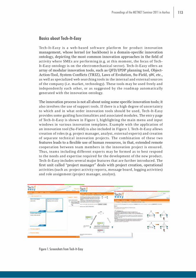
113Proceedings of the METNET Seminar 2011 in Aarhus
Basics about Tech-It-Easy
Tech-It-Easy is a web-based software platform for product innovation management, whose kernel (or backbone) is a domain-specific innovation ontology, depicting the most common innovation approaches in the field of activity where SMEs are performing (e.g. at this moment, the focus of Tech-It-Easy ontology is on the electromechanical sector). Tech-It-Easy offers an array of modular innovation tools, such as QFD/IPDP planning tool, Object-Action-Tool, System Conflicts (TRIZ), Laws of Evolution, Su-Field, 9W, etc., as well as specialized web searching tools in the internal and external sources of the company (i.e. market, technology). These tools may be used freely and independently each other, or as suggested by the roadmap automatically generated with the innovation ontology.
The innovation process is not all about using some specific innovation tools; it also involves the use of support tools. If there is a high degree of uncertainty to which and in what order innovation tools should be used, Tech-It-Easy provides some guiding functionalities and associated modules. The entry page of Tech-It-Easy is shown in Figure 1, highlighting the main menu and input windows in various innovation templates. Example with the application of an innovation tool (Su-Field) is also included in Figure 1. Tech-It-Easy allows creation of roles (e.g. project manager, analyst, external experts) and creation of separate technical innovation projects. The combination of these two features leads to a flexible use of human resources, in that, extended remote cooperation between team members in the innovation project is ensured. Thus, teams including different experts may be formed as to best respond to the needs and expertise required for the development of the new product. Tech-It-Easy includes several major features that are further introduced. The first unit called “project manager” deals with project creation, operational activities (such as: project activity reports, message board, logging activities) and role assignment (project manager, analyst).
members in the innovation project is ensured. Thus, teams including different experts may be formed as to best respond to the needs and expertise required for the development of the new product. Tech-It-Easy includes several major features that are further introduced. The first unit called “project manager” deals with project creation, operational activities (such as: project activity reports, message board, logging activities) and role assignment (project manager, analyst).
Figure 1. Screenshots from Tech-It-Easy The next unit, “activity agent” helps the team members in deciding which innovation tool is appropriate to be used at a certain moment by pointing out the future activities within the innovation process based on a flexible roadmap. The “innovation toolbox” contains the innovation tools to fulfil each innovation activity present in the innovation roadmap. “Document repository” gathers all the technical and marketing electronic documents within the company; documents that are relevant to the innovation process. “Marketing centre” is a supporting tool for managing all market-related information (competitor, competitor products, customers, etc.). “Technical centre” is used to manage all technical related information, such as technical concepts, products, material, technologies, methods, methodologies. The “search module” gets effective access to the internal information repository, as well as to the external knowledge sources (patent databases, web-libraries and web). The “search feature” is enhanced by a “search result processing assistant” that presents to the user a unified result of searches performed on various knowledge bases (internal, web, different patent databases, etc.). The search module comprises also a continuous monitoring system for the technological progress in the areas of interest, by means of a website change tracking feature, thus offering a simplified monitoring system. With the help of these features, the searching and ideation time for appropriate solutions is significantly diminished. Being a web-based software platform, remote collaborative work between the internal team members, external consultants and partners is also possible. Case Study Since the completion of the version 1.0 of the Tech-It-Easy platform (May, 2011), it has been applied in about ten pilot projects from the electromechanical industry for testing and validation. One of these case studies is further exemplified in this paper. It is about the redesign of a measuring head for pressure and flow (Brad and Vaida 2005). The initial version of the sensor (the mechanical part) is shown in Figure 2. The electronic part of the initial sensor is composed of a sinus oscillator, a differential transformer, mono-alternation
Figure 1. Screenshots from Tech-It-Easy
114 Proceedings of the METNET Seminar 2011 in Aarhus
The next unit, “activity agent” helps the team members in deciding which innovation tool is appropriate to be used at a certain moment by pointing out the future activities within the innovation process based on a flexible roadmap. The “innovation toolbox” contains the innovation tools to fulfil each innovation activity present in the innovation roadmap. “Document repository” gathers all the technical and marketing electronic documents within the company; documents that are relevant to the innovation process. “Marketing centre” is a supporting tool for managing all market-related information (competitor, competitor products, customers, etc.). “Technical centre” is used to manage all technical related information, such as technical concepts, products, material, technologies, methods, methodologies. The “search module” gets effective access to the internal information repository, as well as to the external knowledge sources (patent databases, web-libraries and web). The “search feature” is enhanced by a “search result processing assistant” that presents to the user a unified result of searches performed on various knowledge bases (internal, web, different patent databases, etc.). The search module comprises also a continuous monitoring system for the technological progress in the areas of interest, by means of a website change tracking feature, thus offering a simplified monitoring system. With the help of these features, the searching and ideation time for appropriate solutions is significantly diminished. Being a web-based software platform, remote collaborative work between the internal team members, external consultants and partners is also possible.
Case Study
Since the completion of the version 1.0 of the Tech-It-Easy platform (May, 2011), it has been applied in about ten pilot projects from the electromechanical industry for testing and validation. One of these case studies is further exemplified in this paper. It is about the redesign of a measuring head for pressure and flow (Brad and Vaida 2005). The initial version of the sensor (the mechanical part) is shown in Figure 2. The electronic part of the initial sensor is composed of a sinus oscillator, a differential transformer, mono-alternation rectifiers, a differential amplifier, an integrator and a power supply module. All these units are cased in a box of 150 mm x 200 mm x 50 mm. Thus, the electronic unit of the sensor is separated from the mechanical unit. The current production cost of the sensor is 465 €. The need to minimize the electronic unit (target: integration with the mechanical unit), as well as to improve the accuracy of the sensor (from 0.5% (current) to better than 0.3% (target)) is required in order to increase product’s competitiveness. Application of the QFD/IPDP tools from Tech-It-Easy identified the differential amplifier and the coil box as the modules with the highest priority for innovation (see Table 1).
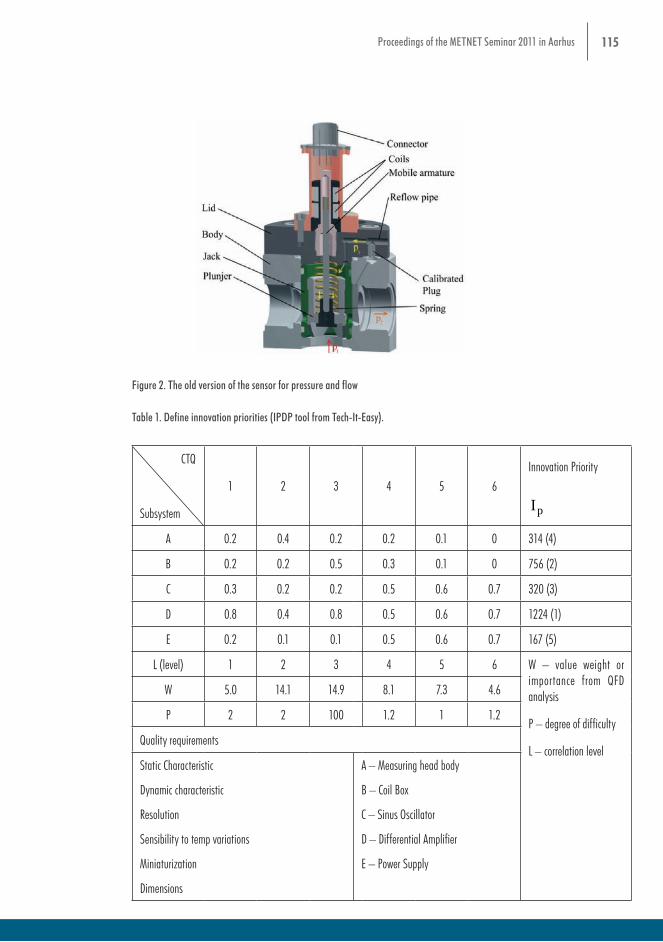
115Proceedings of the METNET Seminar 2011 in Aarhus
rectifiers, a differential amplifier, an integrator and a power supply module. All these units are cased in a box of 150 mm x 200 mm x 50 mm. Thus, the electronic unit of the sensor is separated from the mechanical unit. The current production cost of the sensor is 465 €. The need to minimize the electronic unit (target: integration with the mechanical unit), as well as to improve the accuracy of the sensor (from 0.5% (current) to better than 0.3% (target)) is required in order to increase product’s competitiveness. Application of the QFD/IPDP tools from Tech-It-Easy identified the differential amplifier and the coil box as the modules with the highest priority for innovation (see Table 1).
Figure 2. The old version of the sensor for pressure and flow
CTQ Subsystem
1 2 3 4 5 6 Innovation Priority
pIA 0.2 0.4 0.2 0.2 0.1 0 314 (4)B 0.2 0.2 0.5 0.3 0.1 0 756 (2)C 0.3 0.2 0.2 0.5 0.6 0.7 320 (3)D 0.8 0.4 0.8 0.5 0.6 0.7 1224 (1)E 0.2 0.1 0.1 0.5 0.6 0.7 167 (5)
L (level) 1 2 3 4 5 6 W – value weight or importance from
QFD analysis P – degree of difficulty L – correlation level
W 5.0 14.1 14.9 8.1 7.3 4.6 P 2 2 100 1.2 1 1.2
Quality requirements 1. Static Characteristic 2. Dynamic characteristic 3. Resolution 4. Sensibility to temp variations 5. Miniaturization 6. Dimensions
A – Measuring head body B – Coil Box C – Sinus Oscillator D – Differential Amplifier E – Power Supply
Table 1. Define innovation priorities (IPDP tool from Tech-It-Easy).
The TRIZ tool from Tech-It-Easy identified three conflicting issues that must be over-passed for improving the electronic unit. They are shown in Figure 3.
Figure 2. The old version of the sensor for pressure and flow
Table 1. Define innovation priorities (IPDP tool from Tech-It-Easy).
CTQ
Subsystem
1 2 3 4 5 6Innovation Priority
pI
A 0.2 0.4 0.2 0.2 0.1 0 314 (4)
B 0.2 0.2 0.5 0.3 0.1 0 756 (2)
C 0.3 0.2 0.2 0.5 0.6 0.7 320 (3)
D 0.8 0.4 0.8 0.5 0.6 0.7 1224 (1)
E 0.2 0.1 0.1 0.5 0.6 0.7 167 (5)
L (level) 1 2 3 4 5 6 W – value weight or importance from QFD analysis
P – degree of difficulty
L – correlation level
W 5.0 14.1 14.9 8.1 7.3 4.6
P 2 2 100 1.2 1 1.2
Quality requirements
Static Characteristic
Dynamic characteristic
Resolution
Sensibility to temp variations
Miniaturization
Dimensions
A – Measuring head body
B – Coil Box
C – Sinus Oscillator
D – Differential Amplifier
E – Power Supply
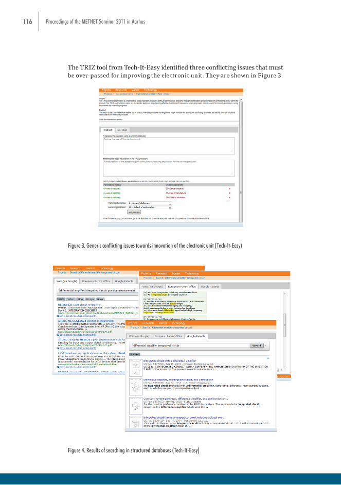
116 Proceedings of the METNET Seminar 2011 in Aarhus
The TRIZ tool from Tech-It-Easy identified three conflicting issues that must be over-passed for improving the electronic unit. They are shown in Figure 3.
Figure 3. Generic conflicting issues towards innovation of the electronic unit (Tech-It-Easy)
Figure 4. Results of searching in structured databases (Tech-It-Easy)
Tech-It-Easy asked searching for solutions which use some materials that lead to the contraction of the system, or to replace the current materials with others, more compact. It was clear; the search direction is towards integrated circuits. Using the searching tool of Tech-It-Easy (see Figure 4), it was possible to replace the classical differential amplifier with an integrated circuit from Philips (NE/SA/5521). For the coil box, Tech-It-Easy recommended searching for solutions able to separate the components that cause
Figure 3. Generic conflicting issues towards innovation of the electronic unit (Tech-It-Easy)
Figure 3. Generic conflicting issues towards innovation of the electronic unit (Tech-It-Easy)
Figure 4. Results of searching in structured databases (Tech-It-Easy)
Tech-It-Easy asked searching for solutions which use some materials that lead to the contraction of the system, or to replace the current materials with others, more compact. It was clear; the search direction is towards integrated circuits. Using the searching tool of Tech-It-Easy (see Figure 4), it was possible to replace the classical differential amplifier with an integrated circuit from Philips (NE/SA/5521). For the coil box, Tech-It-Easy recommended searching for solutions able to separate the components that cause
Figure 4. Results of searching in structured databases (Tech-It-Easy)
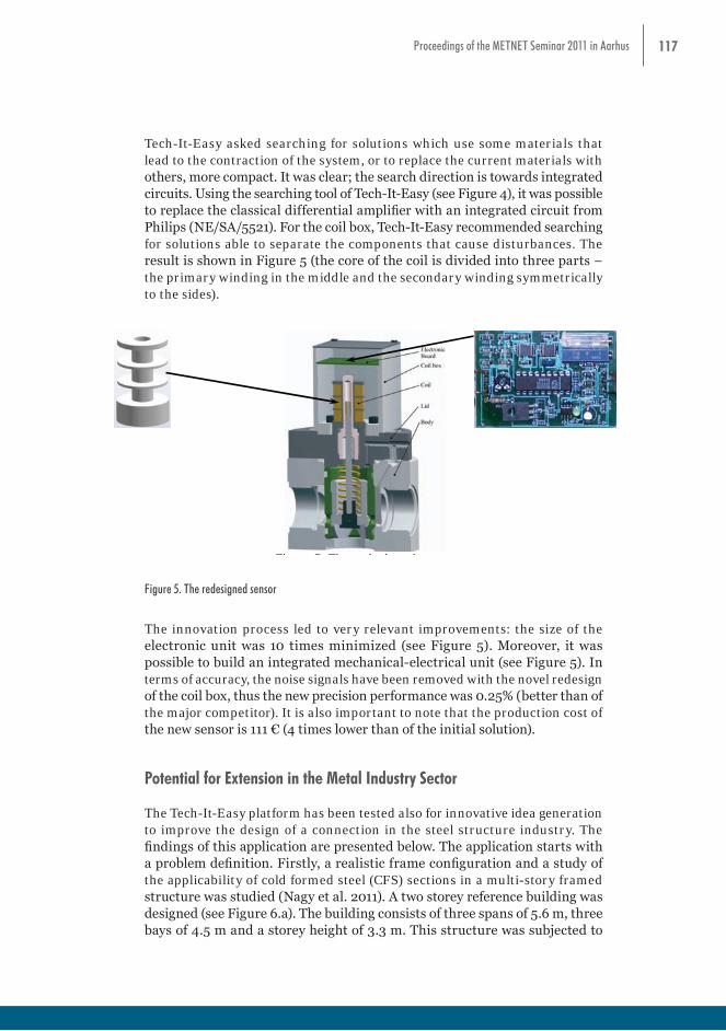
117Proceedings of the METNET Seminar 2011 in Aarhus
Tech-It-Easy asked searching for solutions which use some materials that lead to the contraction of the system, or to replace the current materials with others, more compact. It was clear; the search direction is towards integrated circuits. Using the searching tool of Tech-It-Easy (see Figure 4), it was possible to replace the classical differential amplifier with an integrated circuit from Philips (NE/SA/5521). For the coil box, Tech-It-Easy recommended searching for solutions able to separate the components that cause disturbances. The result is shown in Figure 5 (the core of the coil is divided into three parts – the primary winding in the middle and the secondary winding symmetrically to the sides). disturbances. The result is shown in Figure 5 (the core of the coil is divided into three parts
– the primary winding in the middle and the secondary winding symmetrically to the sides).
Figure 5. The redesigned sensor
The innovation process led to very relevant improvements: the size of the electronic unit was 10 times minimized (see Figure 5). Moreover, it was possible to build an integrated mechanical-electrical unit (see Figure 5). In terms of accuracy, the noise signals have been removed with the novel redesign of the coil box, thus the new precision performance was 0.25% (better than of the major competitor). It is also important to note that the production cost of the new sensor is 111 € (4 times lower than of the initial solution). Potential for Extension in the Metal Industry Sector The Tech-It-Easy platform has been tested also for innovative idea generation to improve the design of a connection in the steel structure industry. The findings of this application are presented below. The application starts with a problem definition. Firstly, a realistic frame configuration and a study of the applicability of cold formed steel (CFS) sections in a multi-story framed structure was studied (Nagy et al. 2011). A two storey reference building was designed (see Figure 6.a). The building consists of three spans of 5.6 m, three bays of 4.5 m and a storey height of 3.3 m. This structure was subjected to loads common in the Romanian structural design practice. The frame was analysed and designed according to EN 1993-1-1 and EN 1993-1-3.
a.
b.
Figure 6. Reference structure (a) and structural model frames with bracings (b)
Figure 5. The redesigned sensor
The innovation process led to very relevant improvements: the size of the electronic unit was 10 times minimized (see Figure 5). Moreover, it was possible to build an integrated mechanical-electrical unit (see Figure 5). In terms of accuracy, the noise signals have been removed with the novel redesign of the coil box, thus the new precision performance was 0.25% (better than of the major competitor). It is also important to note that the production cost of the new sensor is 111 € (4 times lower than of the initial solution).
Potential for Extension in the Metal Industry Sector
The Tech-It-Easy platform has been tested also for innovative idea generation to improve the design of a connection in the steel structure industry. The findings of this application are presented below. The application starts with a problem definition. Firstly, a realistic frame configuration and a study of the applicability of cold formed steel (CFS) sections in a multi-story framed structure was studied (Nagy et al. 2011). A two storey reference building was designed (see Figure 6.a). The building consists of three spans of 5.6 m, three bays of 4.5 m and a storey height of 3.3 m. This structure was subjected to

118 Proceedings of the METNET Seminar 2011 in Aarhus
loads common in the Romanian structural design practice. The frame was analysed and designed according to EN 1993-1-1 and EN 1993-1-3.
disturbances. The result is shown in Figure 5 (the core of the coil is divided into three parts – the primary winding in the middle and the secondary winding symmetrically to the sides).
Figure 5. The redesigned sensor
The innovation process led to very relevant improvements: the size of the electronic unit was 10 times minimized (see Figure 5). Moreover, it was possible to build an integrated mechanical-electrical unit (see Figure 5). In terms of accuracy, the noise signals have been removed with the novel redesign of the coil box, thus the new precision performance was 0.25% (better than of the major competitor). It is also important to note that the production cost of the new sensor is 111 € (4 times lower than of the initial solution). Potential for Extension in the Metal Industry Sector The Tech-It-Easy platform has been tested also for innovative idea generation to improve the design of a connection in the steel structure industry. The findings of this application are presented below. The application starts with a problem definition. Firstly, a realistic frame configuration and a study of the applicability of cold formed steel (CFS) sections in a multi-story framed structure was studied (Nagy et al. 2011). A two storey reference building was designed (see Figure 6.a). The building consists of three spans of 5.6 m, three bays of 4.5 m and a storey height of 3.3 m. This structure was subjected to loads common in the Romanian structural design practice. The frame was analysed and designed according to EN 1993-1-1 and EN 1993-1-3.
a.
b.
Figure 6. Reference structure (a) and structural model frames with bracings (b)
Figure 6. Reference structure (a) and structural model frames with bracings (b)
Once the design of the structure is finished, the problem is to define the structural joints for the selected column and beam sections in that way to obtain both speed in erection (assembly/de-assembly) and cost efficiency for the joints, as well as structural performance, which is defined by the mechanical properties of the joints (Figure 6.b). To solve the structural performance, an initial joining solution was generated (Figure 7). However, some conflicts occur: speed in erection increases the cost efficiency but reduces the structural performance; structural performance improvement has a cost increasing and a reduced speed in erection. To improve the cost efficiency and speed of construction, the inventive principles module of the Tech-It-Easy platform has been used.
Once the design of the structure is finished, the problem is to define the structural joints for the selected column and beam sections in that way to obtain both speed in erection (assembly/de-assembly) and cost efficiency for the joints, as well as structural performance, which is defined by the mechanical properties of the joints (Figure 6.b). To solve the structural performance, an initial joining solution was generated (Figure 7). However, some conflicts occur: speed in erection increases the cost efficiency but reduces the structural performance; structural performance improvement has a cost increasing and a reduced speed in erection. To improve the cost efficiency and speed of construction, the inventive principles module of the Tech-It-Easy platform has been used.
a. SHS section for columns and back-to-back lipped channel sections for beams
b. Strengthened column trough the height of the beam joint – for higher seismic areas
Figure 7. Startup joint typologies
Tech-It-Easy proposed some innovative tips for design improvement like: actions in advance, composite units, segmentation, transition to symmetry, etc. The practical approaches found here are: use pre-fabricated independent parts, use independent parts, and use similar composite parts (see Figure 8). Using these solutions, the cost efficiency and speed of construction for the developed joints can be incrementally improved.
Initial non-symmetric parts Transition to symmetry Transition to segmentation
Figure 8. Joint improvement using innovative principles (Tech-It-Easy)
Final idea Joint configuration
Figure 9. Developed joints to be tested in laboratory
Figure 7. Startup joint typologies
Tech-It-Easy proposed some innovative tips for design improvement like: actions in advance, composite units, segmentation, transition to symmetry, etc. The practical approaches found here are: use pre-fabricated independent parts, use independent parts, and use similar composite parts (see Figure 8). Using these solutions, the cost efficiency and speed of construction for the developed joints can be incrementally improved.
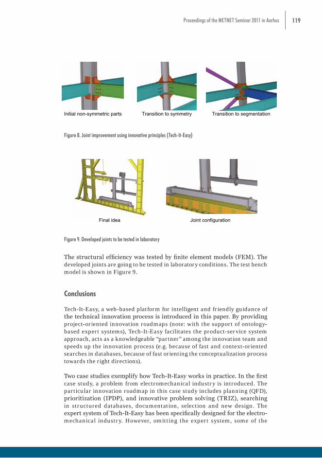
119Proceedings of the METNET Seminar 2011 in Aarhus
Once the design of the structure is finished, the problem is to define the structural joints for the selected column and beam sections in that way to obtain both speed in erection (assembly/de-assembly) and cost efficiency for the joints, as well as structural performance, which is defined by the mechanical properties of the joints (Figure 6.b). To solve the structural performance, an initial joining solution was generated (Figure 7). However, some conflicts occur: speed in erection increases the cost efficiency but reduces the structural performance; structural performance improvement has a cost increasing and a reduced speed in erection. To improve the cost efficiency and speed of construction, the inventive principles module of the Tech-It-Easy platform has been used.
a. SHS section for columns and back-to-back lipped channel sections for beams
b. Strengthened column trough the height of the beam joint – for higher seismic areas
Figure 7. Startup joint typologies
Tech-It-Easy proposed some innovative tips for design improvement like: actions in advance, composite units, segmentation, transition to symmetry, etc. The practical approaches found here are: use pre-fabricated independent parts, use independent parts, and use similar composite parts (see Figure 8). Using these solutions, the cost efficiency and speed of construction for the developed joints can be incrementally improved.
Initial non-symmetric parts Transition to symmetry Transition to segmentation
Figure 8. Joint improvement using innovative principles (Tech-It-Easy)
Final idea Joint configuration
Figure 9. Developed joints to be tested in laboratory
Figure 8. Joint improvement using innovative principles (Tech-It-Easy)
Once the design of the structure is finished, the problem is to define the structural joints for the selected column and beam sections in that way to obtain both speed in erection (assembly/de-assembly) and cost efficiency for the joints, as well as structural performance, which is defined by the mechanical properties of the joints (Figure 6.b). To solve the structural performance, an initial joining solution was generated (Figure 7). However, some conflicts occur: speed in erection increases the cost efficiency but reduces the structural performance; structural performance improvement has a cost increasing and a reduced speed in erection. To improve the cost efficiency and speed of construction, the inventive principles module of the Tech-It-Easy platform has been used.
a. SHS section for columns and back-to-back lipped channel sections for beams
b. Strengthened column trough the height of the beam joint – for higher seismic areas
Figure 7. Startup joint typologies
Tech-It-Easy proposed some innovative tips for design improvement like: actions in advance, composite units, segmentation, transition to symmetry, etc. The practical approaches found here are: use pre-fabricated independent parts, use independent parts, and use similar composite parts (see Figure 8). Using these solutions, the cost efficiency and speed of construction for the developed joints can be incrementally improved.
Initial non-symmetric parts Transition to symmetry Transition to segmentation
Figure 8. Joint improvement using innovative principles (Tech-It-Easy)
Final idea Joint configuration
Figure 9. Developed joints to be tested in laboratory
Figure 9. Developed joints to be tested in laboratory
The structural efficiency was tested by finite element models (FEM). The developed joints are going to be tested in laboratory conditions. The test bench model is shown in Figure 9.
Conclusions
Tech-It-Easy, a web-based platform for intelligent and friendly guidance of the technical innovation process is introduced in this paper. By providing project-oriented innovation roadmaps (note: with the support of ontology-based expert systems), Tech-It-Easy facilitates the product-service system approach, acts as a knowledgeable “partner” among the innovation team and speeds up the innovation process (e.g. because of fast and context-oriented searches in databases, because of fast orienting the conceptualization process towards the right directions).
Two case studies exemplify how Tech-It-Easy works in practice. In the first case study, a problem from electromechanical industry is introduced. The particular innovation roadmap in this case study includes planning (QFD), prioritization (IPDP), and innovative problem solving (TRIZ), searching in structured databases, documentation, selection and new design. The expert system of Tech-It-Easy has been specifically designed for the electro-mechanical industry. However, omitting the expert system, some of the
120 Proceedings of the METNET Seminar 2011 in Aarhus
Tech-It-Easy tools can be also used in other sectors to support innovation. Therefore, Tech-It-Easy has been tested in the steel industry, too; specifically, the structural joint innovation process. In the problem under consideration, multiple TRIZ defines the innovation roadmap. The generated results show a potential for expanding Tech-It-Easy to steel industry. But to make Tech-It-Easy more effective in this sector, further researches and developments are necessary to build customized ontologies for the market and technology search tools, as well as for the product innovation tools (e.g. databases with illustrative case studies) that are specific to steel industry.
Acknowledgements
Financial support from the European Commission, within the FP7 research project TECH-IT-EASY/232410, is acknowledged with gratitude. Tech-It-Easy software platform has been developed by a consortium of RDTs performers, including the work-package leader Technical University of Cluj-Napoca, Research Centre in Engineering and Management of Innovation, Romania; Open University, Knowledge Media Institute, England; Kufstein University of Applied Sciences, Austria; and CIAOTECH srl (member of PNO Group Europe), Italy.
References
Barczak G., Sultan F., Hultink E.J., 2007. Determinants of IT Usage and New Product Performance, Journal of Product Innovation Management, Volume 24, pp. 600–613.
Becattini N., Borgianni Y., Cascini G., 2011. Model and Algorithm for Computer-Aided Inventive Problem Analysis, Computer-Aided Design, 2011, Elsevier.
Bhatt G., Emdad A., Roberts N., Grover V., 2010. Building and Lleveraging Information in Dynamic Environments: The role of IT infrastructure Flexibility as Enabler of Organizational Responsiveness and Competitive Advantage, Information & Management, Volume 47, Issues 7-8, December 2010, pp. 341-349.
Brad S., Vaida C., 2005. Competitive Redesign of a Measuring Head for Pressure and Flow, microCAD International Conference, March 2005, Miskolc, Hungary, pp. 19-24.
Brad S., 2009. Perspectives on High-Tech Product Design for Better Supporting Product-Service Systems, In Proceedings of the 2009 Winter Simulation Conference, Austin, USA, ISBN: 978-1-4244-5771-7/09/IEEE Catalog no.: CFP09WSC-CDR, Library of Congress: 87-654182, pp. 3036-3046, DOI: 10.1109/WSC.2009.5429270.
121Proceedings of the METNET Seminar 2011 in Aarhus
Brad S., Fulea M., Brad E., 2010. A PSS Approach in Software Development, In Proceedings of the 2nd CIRP IPS2 Conference on Industrial Product-Service Systems, Linköping, Sweden, pp. 291-298.
Branzei O., Vertinsky I., 2006. Strategic Pathways to Product Innovation Capabilities in SMEs, Journal of Business Venturing, Volume 21, Issue 1, pp. 75–105.
Clemons D., Kroth M., 2010. Managing the Mobile Workforce: Leading, Building, and Sustaining Virtual Teams, McGraw-Hill Professional; 1 edition.
Fink L., Neumann S., 2007. Gaining Agility through IT Personnel Capabilities: The Mediating Role of IT Infrastructure Capabilities, Journal of the Association for Information Systems, Volume 8, Issue 8, pp. 440–462.
Gunasekaran A., Ngai E.W.T., McGaughey R.E., 2008. Information Technology and Systems Justification, Evaluating Information Systems, Butterworth-Heinemann, Oxford, 2008, pp. 1-34.
Hyeongon W., Seungjin O., Mooyoung J., 2011. Virtual Organization for Open Innovation: Semantic Web Based Inter-organizational Team Formation, Expert Systems with Applications, Volume 38, Issue 7, July 2011, pp. 8466-8476.
Hüsig S., Kohn S., 2009. Computer Aided Innovation-State of the Art from a New Product Development Perspective, Computers in Industry, Volume 60, Issue 8, pp. 551-562.
Kang M.J., Wimmer R., 2008. Product Service Systems as Advanced System Solutions for Sustainability, In Proceedings of the EU-Korea Conference on Science and Technology, ed. S. D. Yoo, pp. 191-199. Heidelberg: Springer-Verlag, Berlin.
Lojeski K.S., 2009. Leading the Virtual Workforce: How Great Leaders Transform Organizations in the 21st Century; John Wiley & Sons (20 Nov 2009).
Malerba F., 2007. Innovation and the Dynamics and Evolution of Industries: Progress and Challenges, International Journal of Industrial Organization, Volume 25, Issue 4, August 2007, pp. 675-699.
Nagy Zs., Dubina D., Ungureanu V., 2011. Application of component method: bolted joints for low rise multi storey cold-formed steel framed structures, In Proceedings of the 6th European Conference on Steel and Composite Structures - Eurosteel 2011, September 2011, pp. 273-278.

122 Proceedings of the METNET Seminar 2011 in Aarhus
Rosenbusch N., Brinckmann J., Bausch A., 2011. Is Innovation Always Beneficial? A Meta-analysis of the Relationship Between Innovation and Performance in SMEs, Journal of Business Venturing, Volume 26, Issue 4, July 2011, pp. 441-457, DOI: 10.1016 /j.jbusvent.2009.12.002.
Solomom C., 2001, Managing Virtual Teams, Workforce, Volume 80, Issue 6, pp. 60–65.
Schwarz E., Krajger I., Dummer R., 2006. Innovationskompass für klein-und mittelständische Unternehmen. Neue Ideen finden und entwickeln; Linde, Wien; Auflage: 1., Aufl. (2006).
Tukker A., Tischner U., 2006. Product-services as a Research Field: Past, Present and Future. Reflections from a Decade of Research, Journal of Cleaner Production, Volume 14, Issue 17, pp. 1552-1556.
Yang L.-R., Chen J.-H., Wang H.-W., 2011. Assessing Impacts of Information Technology on Project Success through Knowledge Management Practice, Automation in Construction, In Press, Corrected Proof, Available online 20 July 2011.

123Proceedings of the METNET Seminar 2011 in Aarhus
On the Cost Structures in Steel Construction
Lauri Tenhunen
HAMK University of Applied Sciences
Abstract
This paper examines the cost structures in steel construction. Quite commonly it is argued that steel construction manufacturing benefits from its speed and exactness, which then has direct effects on the costs and profitability of the whole construction project in question. However, little scientific work has been done on the research of the costs structures on any of the production stages so far.
As examples, we have analyzed two typical physical structures in steel construction. The theory of industrial economics, including production theory and the theory of cost functions, is adopted to analyze the costs minimums. This paper represents a kind of “study in method”. The findings may later be examined with statistical data.
The most interesting finding in this paper seems to be the apparent possibility to substitute the amount for needed steel with structural planning work. This is a part of the optimization problems of the construction project manager.
The examples of the paper are used for roughly formulating the mathematical forms for the production structure in those stages. Some theoretical hypothesis can be settled on the basis of the examination to be verified in further research.
Introduction
The neoclassical theory of production, with its assumptions of costless possibilities of substitution and choice of optimal scale, is a suitable tool for the analysis of the long–run development of industrial structure at an aggregate level.1 On the micro level, not much effort has been done to describe company or project level production choices with neoclassical tools. That is why our attempt seems to be unique and it may open gates for fruitful analyzing of cost structures within construction processes.
In this paper, we try to formulate some useful short-term industrial production structures and cost structures for given stages of the steel construction process (assuming other factors to stay unchanged ceteris paribus) by using the analyzing tools of neoclassical industrial economics. The main unchanged factor in the short-term examination is the input level of the company capital equipment, such as machines and facilities. Our analyses will concentrate
1 See, for example, Tenhunen (1990)
124 Proceedings of the METNET Seminar 2011 in Aarhus
on analyses and substitution between different kinds of labor work, such as planning and direct manufacturing work (e.g. erecting, welding or carrying).
The formulation in this paper is based on the technologies described by the Constant Elasticity of Substitution (CES) and the Par (PAR), which both include the so-called Cobb-Douglas technology (CD) as a special case. As the mathematically formulated production structure implies a given mathematical cost structure, this interchange will be utilized in the analysis.2 In the Examples, we will first fit a Cobb-Douglas (CD) type production isoquant to the example data.
On the theory of the firm
In the theory of the firm, the production function expresses the quantity of production, when given amounts of inputs are used within the production. 3
The production function describes the technology, not the economic behaviour. Production function is a given element, however, usually unknown in practice to the company.
Theoretically, a firm may minimize its costs given its production function. In the theory of micro-economics, it can be shown, that a profit maximizing firm always minimizes costs but a cost minimiser does not necessarily maximize profits (simply because the given output might not be the profit maximizing one).
As the a company s cost structure is intimately related to its production process, the costs and the whole cost structure of the company is determined by the production technology and input prices. The costs function, mathematically derived from the production functions, describe the cost minimizing choices at each level of production and input prices.
In the Example, we consider a larger steel construction project with over passing bridges at Lakalaiva area in Tampere, Finland. As inputs, we use on the one hand, the amounts (hours) of structural planning work and on the other hand, other direct manufacturing costs (including ready assembled steel, its industrial manufacturing plus erection). Hourly cost of planning and the experience based cost per erected steel kilogram (in the year 1990) serve as input prices.
The CD isoquants
On a given isoquant Y = B within the manufacturing stage of industrial construction (given the capital input on the short run) and assuming constant returns to scale we have
2 Raval (2011), Rutherford (2002)3 On the theory of the firm as well as the production theory see, for example, Varian (2006)
125Proceedings of the METNET Seminar 2011 in Aarhus
concentrate on analyses and substitution between different kinds of labor work, such as planning and direct manufacturing work (e.g. erecting, welding or carrying). The formulation in this paper is based on the technologies described by the Constant Elasticity of Substitution (CES) and the Par (PAR), which both include the so-called Cobb-Douglas technology (CD) as a special case. As the mathematically formulated production structure implies a given mathematical cost structure, this interchange will be utilized in the analysis (Raval 2011; Rutherford 2002). In the Examples, we will first fit a Cobb-Douglas (CD) type production isoquant to the example data. On the theory of the firm In the theory of the firm, the production function expresses the quantity of production, when given amounts of inputs are used within the production (Varian 2006: on the theory of the firm as well as the production theory). The production function describes the technology, not the economic behaviour. Production function is a given element, however, usually unknown in practice to the company. Theoretically, a firm may minimize its costs given its production function. In the theory of micro-economics, it can be shown, that a profit maximizing firm always minimizes costs but a cost minimiser does not necessarily maximize profits (simply because the given output might not be the profit maximizing one). As the a company`s cost structure is intimately related to its production process, the costs and the whole cost structure of the company is determined by the production technology and input prices. The costs function, mathematically derived from the production functions, describe the cost minimizing choices at each level of production and input prices. In the Example, we consider a larger steel construction project with over passing bridges at Lakalaiva area in Tampere, Finland. As inputs, we use on the one hand, the amounts (hours) of structural planning work and on the other hand, other direct manufacturing costs (including ready assembled steel, its industrial manufacturing plus erection). Hourly cost of planning and the experience based cost per erected steel kilogram (in the year 1990) serve as input prices. The CD isoquants On a given isoquant Y = B within the manufacturing stage of industrial construction (given the capital input on the short run) and assuming constant returns to scale we have (1) * = B
where Y = production
L = welding work D = production planning work A = constant (A > 0) B = constant (B > 0) 0 < < 1 Solving for L we get the formula for the production isoquants
where Y = production L = welding work D = production planning work A = constant (A > 0) B = constant (B > 0) 0 < 𝛂 < 1
Solving for L we get the formula for the production isoquants
(2) L = [(B/A)*D( -1)]1/ (3) L = g*D( -1)/ where (4) g = constant = (B/A)1/ > 0
(Defined by the fixed level of production on the isoquant Y=B). An example – Description of the case When driving to Tampere from the South, the driver comes to the Lakalaiva area, where the over passing bridges have become landmarks. These bridges are made on concrete pillars and the huge beams are made of steel. The construction work took place about 1992-93. The bridges are beautifully formulated and they represent a kind of infrastructural architecture of their time. The degree of precision of the structural planning correlates strongly with the hours used in it. A small amount of planning leads the way to imprecise steel constructions which typically are heavy and strong. A bigger amount of planning may save steel and related handling work (especially in large construction works) but some more costs come from the increased planning work. In the Lakalaiva steel bridge project, the most competitive offer for steel beams was done after a remarkable amount of structural planning work. The total weight of the steel container beams of the cross road bridge S6 is (quite exactly) 335 tons. The total value for the ready erected steel construction modules of the construction project (of bridge S6) was about 4,02 million Finnish Marks (670.000 Euros) in the year 1992 (A-Insinöörit/A-Engineers 12.8.1992). This corresponds to some 1 million Euros in the year 2011. At the cost level of 1992, the cost for one kg of ready erected steel (in the form of containers steel beams) in the project was 2 Euros/kg. We have calculated that the planning hours used in the structural steel planning of bridge S6 have been around 800 hours. Thus the planning costs in the realized version have been some 216.000 Finnish Marks, corresponding to 36.000 Euros in the nominal money level of 1992. The realized total cost for the steel structures (container beams in this case) in the Lakalaiva Cross Road Bridge S6 has been 706.000 Euros in the nominal money level of 1992. From the original documentation it is not evident, how much planning work was invested in the structural planning. Most of the experts of this project are retired already. To be able to calculate the example, we need to make an assumption for this. But in the year 1992, it was widely known among the contractors (such like PPTH Steel Ltd) that the winning solution for the bridge steel structures was based on a structure which was roughly 15-20 % lighter than the competitors had planned and suggested to the builder. The builder in this project was the road council of Häme, which was a local government office situated in Tampere.
AN EXAMPLE
Description of the case
When driving to Tampere from the South, the driver comes to the Lakalaiva area, where the over passing bridges have become landmarks. These bridges are made on concrete pillars and the huge beams are made of steel. The construction work took place about 1992-93. The bridges are beautifully formulated and they represent a kind of infrastructural architecture of their time.
The degree of precision of the structural planning correlates strongly with the hours used in it. A small amount of planning leads the way to imprecise steel constructions which typically are heavy and strong. A bigger amount of planning may save steel and related handling work (especially in large construction works) but some more costs come from the increased planning work.
In the Lakalaiva steel bridge project, the most competitive offer for steel beams was done after a remarkable amount of structural planning work. The total weight of the steel container beams of the cross road bridge S6 is (quite exactly) 335 tons. The total value for the ready erected steel construction modules of the construction project (of bridge S6) was about 4,02 million Finnish Marks (670.000 Euros) in the year 19924. This corresponds to some 4 The numbers come from the original document 12.8.1992 of the planning company
A-Insinöörit Oy (A-Engineers, 1992)
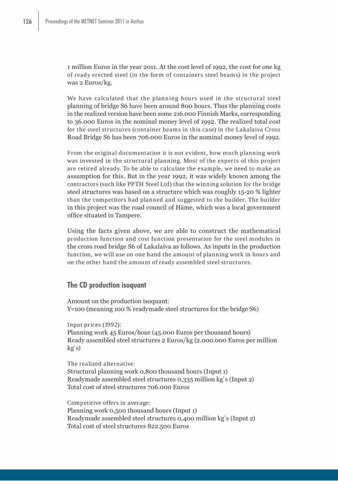
126 Proceedings of the METNET Seminar 2011 in Aarhus
1 million Euros in the year 2011. At the cost level of 1992, the cost for one kg of ready erected steel (in the form of containers steel beams) in the project was 2 Euros/kg.
We have calculated that the planning hours used in the structural steel planning of bridge S6 have been around 800 hours. Thus the planning costs in the realized version have been some 216.000 Finnish Marks, corresponding to 36.000 Euros in the nominal money level of 1992. The realized total cost for the steel structures (container beams in this case) in the Lakalaiva Cross Road Bridge S6 has been 706.000 Euros in the nominal money level of 1992.
From the original documentation it is not evident, how much planning work was invested in the structural planning. Most of the experts of this project are retired already. To be able to calculate the example, we need to make an assumption for this. But in the year 1992, it was widely known among the contractors (such like PPTH Steel Ltd) that the winning solution for the bridge steel structures was based on a structure which was roughly 15-20 % lighter than the competitors had planned and suggested to the builder. The builder in this project was the road council of Häme, which was a local government office situated in Tampere.
Using the facts given above, we are able to construct the mathematical production function and cost function presentation for the steel modules in the cross road bridge S6 of Lakalaiva as follows. As inputs in the production function, we will use on one hand the amount of planning work in hours and on the other hand the amount of ready assembled steel structures.
The CD production isoquant
Amount on the production isoquant: Y=100 (meaning 100 % readymade steel structures for the bridge S6)
Input prices (1992): Planning work 45 Euros/hour (45.000 Euros per thousand hours) Ready assembled steel structures 2 Euros/kg (2.000.000 Euros per million kg s)
The realized alternative: Structural planning work 0,800 thousand hours (Input 1) Readymade assembled steel structures 0,335 million kg s (Input 2) Total cost of steel structures 706.000 Euros
Competitive offers in average: Planning work 0,500 thousand hours (Input 1) Readymade assembled steel structures 0,400 million kg s (Input 2) Total cost of steel structures 822.500 Euros

127Proceedings of the METNET Seminar 2011 in Aarhus
The volume points of the inputs (reference points) are the following: L
0 = 0,800 thousand hours
D0 = 0,335 million kg s
L1 = 0,500 thousand hours
D1 = 0,400 million kg s.
The CD production function form in this case will explicitly be5 (5) Y = 234,2*L0,274*D0,726 And the corresponding cost function will be6 (6) C(Y,w) = 0,007681*Y*wL
0,274*wD0,726
When wL = 45.000, wD = 2.000.000 and Y = 100, we get the cost minimum (7) C(Y,w) ≈ 0,7681*450000,274*20000000,726 ≈ 543.200 Euros. This would take place when we choose the optimal amounts of structural planning work and the readymade steel structures as follows (following Sheppard`s lemma): (8) L = ∂C/∂wL = 0,7681*0,274*wL
0,274-1*wD0,726 = 3,315 thousand hours
(9) D = ∂C/∂wK = 0,7681*0,726* wL
0,274*wD0,7,26-1 = 0,197 million kg`s
The total working costs in the optimum can be divided as follows (10) wL*L = 45000*3,315 = 149.200 Euros
(Income share of structural planning work, 27,4 %)
wD*D = 2000000*0,197 = 394.000 Euros (Income share of readymade steel structures, 72,6 %)
The cost level given by (33) can be verified from the basic cost equation (11) C = wL*L + wD*D = 45000*3,315 + 2000000*0,197 ≈ 543.200 Euros The realized combination in the Example seems to be 706.000 - 543.200 = 162.800 Euros more expensive than the cost minimum (assuming CD technology) would have been.
5 This is solved from a pair of isoquant equations which go through the input reference points. 6 Compare with Border (2009) 5 This is solved from a pair of isoquant equations which go through the input reference points.6 Compare with Border (2009)
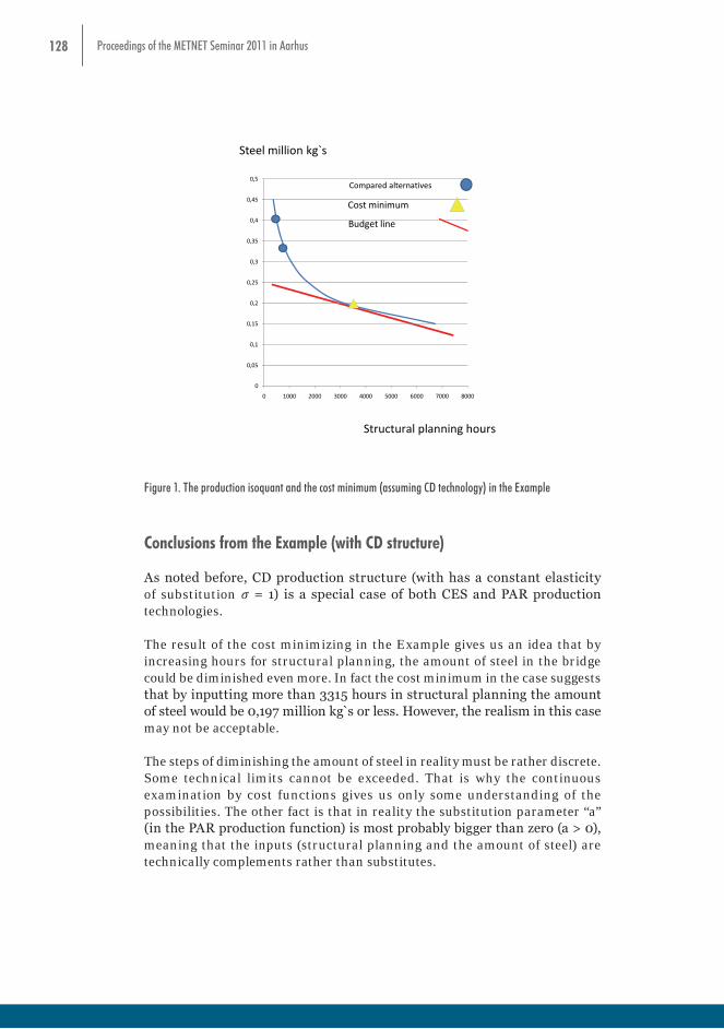
128 Proceedings of the METNET Seminar 2011 in Aarhus
The total working costs in the optimum can be divided as follows (10) wL*L = 45000*3,315 = 149.200 Euros
(Income share of structural planning work, 27,4 %)
wD*D = 2000000*0,197 = 394.000 Euros (Income share of readymade steel structures, 72,6 %)
The cost level given by (33) can be verified from the basic cost equation (11) C = wL*L + wD*D = 45000*3,315 + 2000000*0,197 ≈ 543.200 Euros The realized combination in the Example seems to be 706.000 - 543.200 = 162.800 Euros more expensive than the cost minimum (assuming CD technology) would have been.
0
0,05
0,1
0,15
0,2
0,25
0,3
0,35
0,4
0,45
0,5
0 1000 2000 3000 4000 5000 6000 7000 8000
Steel million kg`s
Structural planning hours
Cost minimum
Compared alternatives
Budget line
Figure 1. The production isoquant and the cost minimum (assuming CD technology) in the Example
Conclusions from the Example (with CD structure) As noted before, CD production structure (with has a constant elasticity of substitution = 1) is a special case of both CES and PAR production technologies. The result of the cost minimizing in the Example gives us an idea that by increasing hours for structural planning, the amount of steel in the bridge could be diminished even more. In fact the cost minimum in the case suggests that by inputting more than 3315 hours in structural planning the amount of steel would be 0,197 million kg`s or less. However, the realism in this case may not be acceptable. The steps of diminishing the amount of steel in reality must be rather discrete. Some technical limits cannot be exceeded. That is why the continuous examination by cost
Figure 1. The production isoquant and the cost minimum (assuming CD technology) in the Example
Conclusions from the Example (with CD structure)
As noted before, CD production structure (with has a constant elasticity of substitution 𝜎 = 1) is a special case of both CES and PAR production technologies.
The result of the cost minimizing in the Example gives us an idea that by increasing hours for structural planning, the amount of steel in the bridge could be diminished even more. In fact the cost minimum in the case suggests that by inputting more than 3315 hours in structural planning the amount of steel would be 0,197 million kg s or less. However, the realism in this case may not be acceptable.
The steps of diminishing the amount of steel in reality must be rather discrete. Some technical limits cannot be exceeded. That is why the continuous examination by cost functions gives us only some understanding of the possibilities. The other fact is that in reality the substitution parameter “a” (in the PAR production function) is most probably bigger than zero (a > 0), meaning that the inputs (structural planning and the amount of steel) are technically complements rather than substitutes.
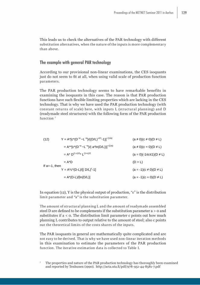
129Proceedings of the METNET Seminar 2011 in Aarhus
This leads us to check the alternatives of the PAR technology with different substitution alternatives, when the nature of the inputs is more complementary than above.
The example with general PAR technology
According to our provisional non-linear examinations, the CES isoquants just do not seem to fit at all, when using valid scale of production function parameters.
The PAR production technology seems to have remarkable benefits in examining the isoquants in this case. The reason is that PAR production functions have such flexible limiting properties which are lacking in the CES technology. That is why we have used the PAR production technology (with constant returns of scale) here, with inputs L (structural planning) and D (readymade steel structures) with the following form of the PAR production function 7
functions gives us only some understanding of the possibilities. The other fact is that in reality the substitution parameter “a” (in the PAR production function) is most probably bigger than zero (a > 0), meaning that the inputs (structural planning and the amount of steel) are technically complements rather than substitutes. This leads us to check the alternatives of the PAR technology with different substitution alternatives, when the nature of the inputs is more complementary than above. The example with general PAR technology According to our provisional non-linear examinations, the CES isoquants just do not seem to fit at all, when using valid scale of production function parameters. The PAR production technology seems to have remarkable benefits in examining the isoquants in this case. The reason is that PAR production functions have such flexible limiting properties which are lacking in the CES technology. That is why we have used the PAR production technology (with constant returns of scale) here, with inputs L (structural planning) and D (readymade steel structures) with the following form of the PAR production function (Tenhunen 1990). (12) Y = A*[c*(D−a −L−a)/((D/L)-a*c-1)]−(1/a) (a ≠ 0)(c ≠ 0)(D ≠ L) = A**[c*(D−a −L−a)/(-a*ln(D/L))]−(1/a) (a ≠ 0)(c = 0)(D ≠ L) = A* D(1-c)/2* L(1+c)/2 (a = 0)(-1≤c≤1)(D ≠ L) = A*D (D = L) If a=-1, then Y = A*c*(D-L)/[( D/L)c-1] (a = -1)(c ≠ 0)(D ≠ L) = A*(D-L)/[ln(D/L)] (a = -1)(c = 0)(D ≠ L) In equation (12), Y is the physical output of production, “c” is the distribution limit parameter and “a” is the substitution parameter. The amount of structural planning L and the amount of readymade assembled steel D are defined to be complements if the substitution parameter a > 0 and substitutes if a < 0. The distribution limit parameter c points out how much planning L contributes to output relative to the amount of steel; also c points out the theoretical limits of the costs shares of the inputs. The PAR isoquants in general are mathematically quite complicated and are not easy to be derived. That is why we have used non-linear iteration methods in this examination to estimate the parameters of the PAR production function. The iterative estimation data is collected to Table 1. Based on the information in Table 1, the optimal level of steel can be drawn as function of the substitution parameter “a” (Figure 5) as well as a function of the distribution limit parameter “c” (Figure 6).
In equation (12), Y is the physical output of production, “c” is the distribution limit parameter and “a” is the substitution parameter.
The amount of structural planning L and the amount of readymade assembled steel D are defined to be complements if the substitution parameter a > 0 and substitutes if a < 0. The distribution limit parameter c points out how much planning L contributes to output relative to the amount of steel; also c points out the theoretical limits of the costs shares of the inputs.
The PAR isoquants in general are mathematically quite complicated and are not easy to be derived. That is why we have used non-linear iteration methods in this examination to estimate the parameters of the PAR production function. The iterative estimation data is collected to Table 1.
7 The properties and nature of the PAR production technology has thoroughly been examined and reported by Tenhunen (1990). http://acta.uta.fi/pdf/978-951-44-8581-7.pdf

130 Proceedings of the METNET Seminar 2011 in Aarhus
Based on the information in Table 1, the optimal level of steel can be drawn as function of the substitution parameter “a” (Figure 5) as well as a function of the distribution limit parameter “c” (Figure 6).
In Figure 7 we have described the situation where the substitution parameter is set to be a=5. The estimate for the the distribution limit parameter is ĉ=-0,0574 and for the scale parameter to be Â=227,4.
Table 1. Cost minimums with different parameters in the PAR production technol
Nature of inputs Substitution parameter a
Distribution limit parameter c
Scale parameter A
Cost share limits for structural steel
min – max (depending on the input ratio)
The cost share of structural steel in the optimum
Optimal level of structural planning hours
Optimal level of structural steel million kgs
Cost minimum Euros
Supplements -0,5 -0,4868 235,9 0,4868 - 1 0,644 3900 0,159 494.000
Supplements -0,1 -0,4593 235,5 0,4593 - 1 0,704 3500 0,187 531.500
Neutral 0 -0,452 235,2 0,726 0,726 3300 0,197 543.200
Complements +0,2 -0,4374 234,9 0,4374 - 1 0,758 3100 0,2095 558.500
Complements +1 -0,375 233,7 0,375 - 1 0,844 2300 0,2538 611.100
Complements +2 -0,2898 231,8 0,2898 - 1 0,875 1800 0,2827 646.420
Complements +3 -0,205 230,2 0,205 - 1 0,891 1600 0,2958 663.580
Complements +5 -0,0574 227,4 0,0574 - 1 0,9 1500 0,3033 674.100
Complements +8 0,0872 225,0 0 – 0,9118 0,878 1800 0,2912 663.450
Complements +11 0,1643 224,2 0 – 0,8357 0,795 2400 0,2637 635.450
Complements +15 0,2154 224,3 0 – 0,7846 0,705 2900 0,2340 598.500
Complements +20 0,2443 225,1 0 – 0.7557 0,756 3100 0,2160 571.500
The realized input combination (not optimum) 0,949 800 0,335 706.000
From Figures 5-9 it can be seen that the optimum amount of structural planning in all analysed cases is bigger than used in the realised situation.
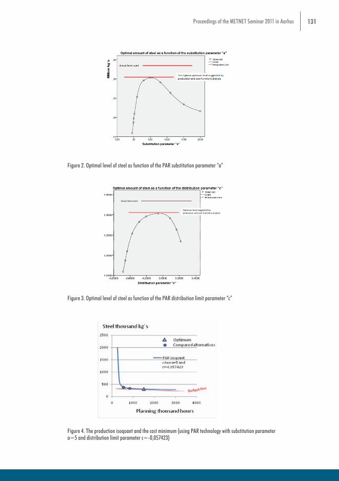
131Proceedings of the METNET Seminar 2011 in Aarhus
In Figure 7 we have described the situation where the substitution parameter is set to be a=5. The estimate for the the distribution limit parameter is ĉ=-0,0574 and for the scale parameter to be Â=227,4.
Table 1. Cost minimums with different parameters in the PAR production technology Nature of inputs Substitution
parameter a Distribution
limit parameter c
Scale parameter
A
Cost share limits for structural
steel min – max
(depending on the input ratio)
The cost share of structural
steel in the optimum
Optimal level of
structural planning
hours
Optimal level of
structural steel
million kgs
Cost minimum
Euros
Supplements -0,5 -0,4868 235,9 0,4868 - 1 0,644 3900 0,159 494.000 Supplements -0,1 -0,4593 235,5 0,4593 - 1 0,704 3500 0,187 531.500 Neutral 0 -0,452 235,2 0,726 0,726 3300 0,197 543.200 Complements +0,2 -0,4374 234,9 0,4374 - 1 0,758 3100 0,2095 558.500 Complements +1 -0,375 233,7 0,375 - 1 0,844 2300 0,2538 611.100 Complements +2 -0,2898 231,8 0,2898 - 1 0,875 1800 0,2827 646.420 Complements +3 -0,205 230,2 0,205 - 1 0,891 1600 0,2958 663.580 Complements +5 -0,0574 227,4 0,0574 - 1 0,9 1500 0,3033 674.100 Complements +8 0,0872 225,0 0 – 0,9118 0,878 1800 0,2912 663.450 Complements +11 0,1643 224,2 0 – 0,8357 0,795 2400 0,2637 635.450 Complements +15 0,2154 224,3 0 – 0,7846 0,705 2900 0,2340 598.500 Complements +20 0,2443 225,1 0 – 0.7557 0,756 3100 0,2160 571.500
The realized input combination (not optimum) 0,949 800 0,335 706.000 From Figures 5-9 it can be seen that the optimum amount of structural planning in all analysed cases is bigger than used in the realised situation.
Figure 2. Optimal level of steel as function of the PAR substitution parameter “a”
Optimum level suggested byproduction and cost functions analysis
Actual level used
Figure 3. Optimal level of steel as function of the PAR distribution limit parameter “c”
Figure 2. Optimal level of steel as function of the PAR substitution parameter “a”
In Figure 7 we have described the situation where the substitution parameter is set to be a=5. The estimate for the the distribution limit parameter is ĉ=-0,0574 and for the scale parameter to be Â=227,4.
Table 1. Cost minimums with different parameters in the PAR production technology Nature of inputs Substitution
parameter a Distribution
limit parameter c
Scale parameter
A
Cost share limits for structural
steel min – max
(depending on the input ratio)
The cost share of structural
steel in the optimum
Optimal level of
structural planning
hours
Optimal level of
structural steel
million kgs
Cost minimum
Euros
Supplements -0,5 -0,4868 235,9 0,4868 - 1 0,644 3900 0,159 494.000 Supplements -0,1 -0,4593 235,5 0,4593 - 1 0,704 3500 0,187 531.500 Neutral 0 -0,452 235,2 0,726 0,726 3300 0,197 543.200 Complements +0,2 -0,4374 234,9 0,4374 - 1 0,758 3100 0,2095 558.500 Complements +1 -0,375 233,7 0,375 - 1 0,844 2300 0,2538 611.100 Complements +2 -0,2898 231,8 0,2898 - 1 0,875 1800 0,2827 646.420 Complements +3 -0,205 230,2 0,205 - 1 0,891 1600 0,2958 663.580 Complements +5 -0,0574 227,4 0,0574 - 1 0,9 1500 0,3033 674.100 Complements +8 0,0872 225,0 0 – 0,9118 0,878 1800 0,2912 663.450 Complements +11 0,1643 224,2 0 – 0,8357 0,795 2400 0,2637 635.450 Complements +15 0,2154 224,3 0 – 0,7846 0,705 2900 0,2340 598.500 Complements +20 0,2443 225,1 0 – 0.7557 0,756 3100 0,2160 571.500
The realized input combination (not optimum) 0,949 800 0,335 706.000 From Figures 5-9 it can be seen that the optimum amount of structural planning in all analysed cases is bigger than used in the realised situation.
Figure 2. Optimal level of steel as function of the PAR substitution parameter “a”
Optimum level suggested byproduction and cost functions analysis
Actual level used
Figure 3. Optimal level of steel as function of the PAR distribution limit parameter “c”
Figure 3. Optimal level of steel as function of the PAR distribution limit parameter “c”
Figure 4. The production isoquant and the cost minimum (using PAR technology with substitution parameter
a=5 and distribution limit parameter c=-0,057423)
Thelowest optimum level suggested byproduction and cost functions analysis
Actual level used
Figure 5. Optimal level of structural planning as function of the PAR substitution parameter “a”
Thelowest optimum level suggested byproduction and cost functions analysis
Actual level used
Figure 6. Optimal level of structural planning as function of the PAR distribution limit parameter “c”
Conclusions from the example with general PAR technology From Table 1 and Figures 2-9 it can be seen e.g. that
Figure 4. The production isoquant and the cost minimum (using PAR technology with substitution parameter a=5 and distribution limit parameter c=-0,057423)

132 Proceedings of the METNET Seminar 2011 in Aarhus
Figure 4. The production isoquant and the cost minimum (using PAR technology with substitution parameter
a=5 and distribution limit parameter c=-0,057423)
Thelowest optimum level suggested byproduction and cost functions analysis
Actual level used
Figure 5. Optimal level of structural planning as function of the PAR substitution parameter “a”
Thelowest optimum level suggested byproduction and cost functions analysis
Actual level used
Figure 6. Optimal level of structural planning as function of the PAR distribution limit parameter “c”
Conclusions from the example with general PAR technology From Table 1 and Figures 2-9 it can be seen e.g. that
Figure 5. Optimal level of structural planning as function of the PAR substitution parameter “a”
Figure 4. The production isoquant and the cost minimum (using PAR technology with substitution parameter
a=5 and distribution limit parameter c=-0,057423)
Thelowest optimum level suggested byproduction and cost functions analysis
Actual level used
Figure 5. Optimal level of structural planning as function of the PAR substitution parameter “a”
Thelowest optimum level suggested byproduction and cost functions analysis
Actual level used
Figure 6. Optimal level of structural planning as function of the PAR distribution limit parameter “c”
Conclusions from the example with general PAR technology From Table 1 and Figures 2-9 it can be seen e.g. that
Figure 6. Optimal level of structural planning as function of the PAR distribution limit parameter “c”
Conclusions from the example with general PAR technology
From Table 1 and Figures 2-9 it can be seen e.g. that
• The highest optimal level of steel in the example case is around 303 tons of steel, which is the case where the substitution parameter a≈5. This is the case also when the distribution limit parameter c≈-0,05. The optimal level is clearly less than used in the actual situation (actual level was some 335 tons of steel).
• In all of the examined cases, a higher amount of structural planning would have been cost effective, and it would have caused a lower cost level for the project. The lowest level of structural planning (1500
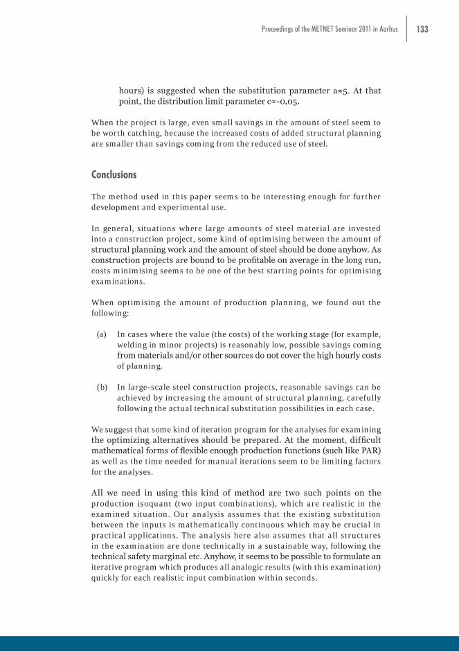
133Proceedings of the METNET Seminar 2011 in Aarhus
Figure 4. The production isoquant and the cost minimum (using PAR technology with substitution parameter
a=5 and distribution limit parameter c=-0,057423)
Thelowest optimum level suggested byproduction and cost functions analysis
Actual level used
Figure 5. Optimal level of structural planning as function of the PAR substitution parameter “a”
Thelowest optimum level suggested byproduction and cost functions analysis
Actual level used
Figure 6. Optimal level of structural planning as function of the PAR distribution limit parameter “c”
Conclusions from the example with general PAR technology From Table 1 and Figures 2-9 it can be seen e.g. that
Figure 5. Optimal level of structural planning as function of the PAR substitution parameter “a”
Figure 4. The production isoquant and the cost minimum (using PAR technology with substitution parameter
a=5 and distribution limit parameter c=-0,057423)
Thelowest optimum level suggested byproduction and cost functions analysis
Actual level used
Figure 5. Optimal level of structural planning as function of the PAR substitution parameter “a”
Thelowest optimum level suggested byproduction and cost functions analysis
Actual level used
Figure 6. Optimal level of structural planning as function of the PAR distribution limit parameter “c”
Conclusions from the example with general PAR technology From Table 1 and Figures 2-9 it can be seen e.g. that
Figure 6. Optimal level of structural planning as function of the PAR distribution limit parameter “c”
Conclusions from the example with general PAR technology
From Table 1 and Figures 2-9 it can be seen e.g. that
• The highest optimal level of steel in the example case is around 303 tons of steel, which is the case where the substitution parameter a≈5. This is the case also when the distribution limit parameter c≈-0,05. The optimal level is clearly less than used in the actual situation (actual level was some 335 tons of steel).
• In all of the examined cases, a higher amount of structural planning would have been cost effective, and it would have caused a lower cost level for the project. The lowest level of structural planning (1500
hours) is suggested when the substitution parameter a≈5. At that point, the distribution limit parameter c≈-0,05.
When the project is large, even small savings in the amount of steel seem to be worth catching, because the increased costs of added structural planning are smaller than savings coming from the reduced use of steel.
Conclusions
The method used in this paper seems to be interesting enough for further development and experimental use.
In general, situations where large amounts of steel material are invested into a construction project, some kind of optimising between the amount of structural planning work and the amount of steel should be done anyhow. As construction projects are bound to be profitable on average in the long run, costs minimising seems to be one of the best starting points for optimising examinations.
When optimising the amount of production planning, we found out the following:
(a) In cases where the value (the costs) of the working stage (for example, welding in minor projects) is reasonably low, possible savings coming from materials and/or other sources do not cover the high hourly costs of planning.
(b) In large-scale steel construction projects, reasonable savings can be achieved by increasing the amount of structural planning, carefully following the actual technical substitution possibilities in each case.
We suggest that some kind of iteration program for the analyses for examining the optimizing alternatives should be prepared. At the moment, difficult mathematical forms of flexible enough production functions (such like PAR) as well as the time needed for manual iterations seem to be limiting factors for the analyses.
All we need in using this kind of method are two such points on the production isoquant (two input combinations), which are realistic in the examined situation. Our analysis assumes that the existing substitution between the inputs is mathematically continuous which may be crucial in practical applications. The analysis here also assumes that all structures in the examination are done technically in a sustainable way, following the technical safety marginal etc. Anyhow, it seems to be possible to formulate an iterative program which produces all analogic results (with this examination) quickly for each realistic input combination within seconds.
134 Proceedings of the METNET Seminar 2011 in Aarhus
References
A-Engineers (1992) Costs calculations of the Lakalaiva cross road bridge S6. A-Insinöörit 12.8.1992 / Juha Ilveskoski, Tampere, Finland.
Border, K.C. (2009) Examples of Cost and Production Functions. California Institute of Technology. www.hss.caltech.edu/~kcb/Notes/CostFunctionExamples.pdf (20.8.2011)
Raval, Devesh (2011) Beyond Cobb-Douglas: Estimation of a CES Production Function with Factor Augmenting Technology. University of Chicago, 2011.
Rutherford, Thomas, F. (2002) Lecture Notes on Constant Elasticity Functions. University of Colorado, 2002.
Tenhunen, Lauri (1990) The CES and Par production Techniques, Income Distribution and the Neoclassical Theory of Production. Tampere 1990. http://acta.uta.fi/pdf/978-951-44-8581-7.pdf
Varian, Hal R. (2006) Intermediate microeconomics, 7th Ed. ISE. New York, 2006.

135Proceedings of the METNET Seminar 2011 in Aarhus
TECHNICAL NOTES

136 Proceedings of the METNET Seminar 2011 in Aarhus
POTENTIALLY PLASTIC ZONES CONFIGURATIONS IN BOTTOM COLUMNS OF ECCENTRICALLY BRACED
FRAMES
Helmuth Köber
Bogdan Ştefănescu
Şerban Dima
Steel Structures Department,
Technical University of Civil Engineering Bucharest, Bucharest, Romania
Abstract
The achievement of a favourable global failure mechanism for eccentrically braced frames presumes the occurrence of plastic deformations at the bottom end of all first-story braces and columns, after plastifying of all dissipative members.
The present paper is intended to illustrate the advantages and disadvantages of different structural details for the potentially plastic zones located near the bottom end of the columns. Several structural details were analyzed considering: reduced flanges cross-sections and/or transversal and longitudinal stiffeners for the bottom zone of the columns.
Two eccentrically braced frames were considered for the analyses. The geometry of the analyzed frames is given in the figure below:
POTENTIALLY PLASTIC ZONES CONFIGURATIONS IN BOTTOM COLUMNS OF ECCENTRICALLY BRACED FRAMES
Helmuth Köber Bogdan Ştefănescu
Şerban Dima
Steel Structures Department, Technical University of Civil Engineering Bucharest, Bucharest, Romania
Abstract The achievement of a favourable global failure mechanism for eccentrically braced frames presumes the occurrence of plastic deformations at the bottom end of all first-story braces and columns, after plastifying of all dissipative members. The present paper is intended to illustrate the advantages and disadvantages of different structural details for the potentially plastic zones located near the bottom end of the columns. Several structural details were analyzed considering: reduced flanges cross-sections and/or transversal and longitudinal stiffeners for the bottom zone of the columns. Two eccentrically braced frames were considered for the analyses. The geometry of the analyzed frames is given in the figure below:
Figure 1. Analyzed eccentrically braced frames
Dynamic nonlinear analyses were performed for each structural configuration. The N-S component of the Vrancea 1977 earthquake acceleration record was used [1]. The acceleration record was calibrated to a peak ground acceleration value of approximately
Figure 1. Analyzed eccentrically braced frames
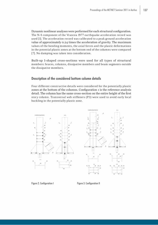
137Proceedings of the METNET Seminar 2011 in Aarhus
POTENTIALLY PLASTIC ZONES CONFIGURATIONS IN BOTTOM COLUMNS OF ECCENTRICALLY BRACED
FRAMES
Helmuth Köber
Bogdan Ştefănescu
Şerban Dima
Steel Structures Department,
Technical University of Civil Engineering Bucharest, Bucharest, Romania
Abstract
The achievement of a favourable global failure mechanism for eccentrically braced frames presumes the occurrence of plastic deformations at the bottom end of all first-story braces and columns, after plastifying of all dissipative members.
The present paper is intended to illustrate the advantages and disadvantages of different structural details for the potentially plastic zones located near the bottom end of the columns. Several structural details were analyzed considering: reduced flanges cross-sections and/or transversal and longitudinal stiffeners for the bottom zone of the columns.
Two eccentrically braced frames were considered for the analyses. The geometry of the analyzed frames is given in the figure below:
Figure 1. Analyzed eccentrically braced frames
Dynamic nonlinear analyses were performed for each structural configuration. The N-S component of the Vrancea 1977 earthquake acceleration record was used [1]. The acceleration record was calibrated to a peak ground acceleration value of approximately 0.24 times the acceleration of gravity. The maximum values of the bending moments, the axial forces and the plastic deformations in the potential plastic zones at the bottom end of the columns were compared [7]. No damping was taken into consideration.
Built-up I-shaped cross-sections were used for all types of structural members: braces, columns, dissipative members and beam segments outside the dissipative members.
Description of the considered bottom column details
Four different constructive details were considered for the potentially plastic zones at the bottom of the columns. Configuration 1 is the reference analysis detail. The column has the same cross-section on the entire height of the first story column. Transversal web stiffeners (P3) were used to avoid early local buckling in the potentially plastic zone.
0.24 times the acceleration of gravity. The maximum values of the bending moments, the axial forces and the plastic deformations in the potential plastic zones at the bottom end of the columns were compared [7]. No damping was taken into consideration. Built-up I-shaped cross-sections were used for all types of structural members: braces, columns, dissipative members and beam segments outside the dissipative members. Description of the considered bottom column details Four different constructive details were considered for the potentially plastic zones at the bottom of the columns. Configuration 1 is the reference analysis detail. The column has the same cross-section on the entire height of the first story column. Transversal web stiffeners (P3) were used to avoid early local buckling in the potentially plastic zone.
1 1
1-1
2 2
1 1
2 2
P1P1
P2
P3
P3
P3
P3
P1P1
P2
2-2
P1P1 P3
P3
P2
A-A
P2
P1
P3
P3
P3
P3
CONFIGURATION I
A
A
P3
P3
P3
P3
1 1
1-1
4 4
1 1
3 3
P1P1
P2
P3
P3
P1P1
P2
2-2
A-A
P2
P1
P5
P3
P3
P3
CONFIGURATION II
A
A
P4P5
P1P1
P2
P43-3
P3
2 2 2 2
P1P1
P2
P4 P5
P5
P5P5
P5
P4
P4
P1P1
P2
P44-4
P4
P3
P3
P3
P3
P3P3
P5
3 3
4 4
P3
P3
P3
P3
Figure 2. Configuration I Figure 3. Configuration II
Figure 2. Configuration I Figure 3. Configuration II
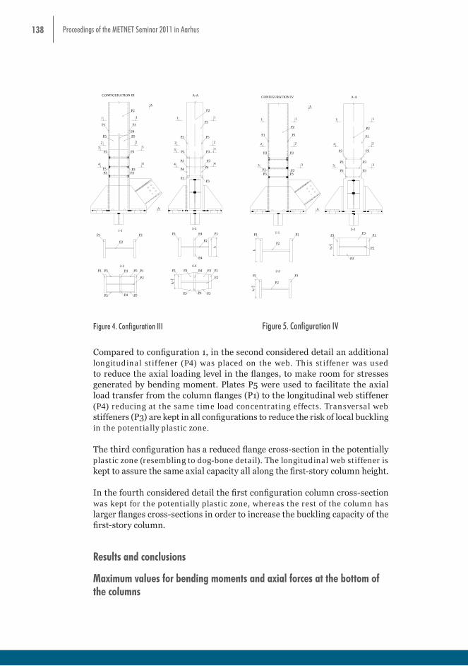
138 Proceedings of the METNET Seminar 2011 in Aarhus
1 1
1-1
4 4
1 1
3 3
P1P1
P2
P3
P3
P1P1
P2
2-2
A-A
P2
P1
P5
P3
P3
P3
CONFIGURATION III
A
A
P4P5
P1P1
P2
P43-3
P3
2 2 2 2
P1P1
P2
P4 P5
P5
P5P5
P5
P4
P4
4-4
P3
P3
P3
P3
P3P3
P5
3 3
4 4P4P4
P1P1
P2
P4
P4 P3
P3
P3
P3
b 1>b 2
b
1 1 1 1
3 3
P1P1
P2
P3
P3
P1P1
P2
2-2
A-A
P2
P1
P3
P3
CONFIGURATION IV
A
A
3-3
P3
2 2 2 2
P3
P3
P3
P3P3
3 3
P3P3
P1P1
P2
1-1P1P1 P3
P3
P2bb 1
>b 2
b 1>b 2
Figure 4. Configuration III Figure 5. Configuration IV Compared to configuration 1, in the second considered detail an additional longitudinal stiffener (P4) was placed on the web. This stiffener was used to reduce the axial loading level in the flanges, to make room for stresses generated by bending moment. Plates P5 were used to facilitate the axial load transfer from the column flanges (P1) to the longitudinal web stiffener (P4) reducing at the same time load concentrating effects. Transversal web stiffeners (P3) are kept in all configurations to reduce the risk of local buckling in the potentially plastic zone. The third configuration has a reduced flange cross-section in the potentially plastic zone (resembling to dog-bone detail). The longitudinal web stiffener is kept to assure the same axial capacity all along the first-story column height. In the fourth considered detail the first configuration column cross-section was kept for the potentially plastic zone, whereas the rest of the column has larger flanges cross-sections in order to increase the buckling capacity of the first-story column. Results and conclusions Maximum values for bending moments and axial forces at the bottom of the columns Configuration 3 (with reduced column flanges in the potentially plastic zones) leads to the smallest bending moment values at the bottom end of the first-story columns.
Figure 4. Configuration III Figure 5. Configuration IV
Compared to configuration 1, in the second considered detail an additional longitudinal stiffener (P4) was placed on the web. This stiffener was used to reduce the axial loading level in the flanges, to make room for stresses generated by bending moment. Plates P5 were used to facilitate the axial load transfer from the column flanges (P1) to the longitudinal web stiffener (P4) reducing at the same time load concentrating effects. Transversal web stiffeners (P3) are kept in all configurations to reduce the risk of local buckling in the potentially plastic zone.
The third configuration has a reduced flange cross-section in the potentially plastic zone (resembling to dog-bone detail). The longitudinal web stiffener is kept to assure the same axial capacity all along the first-story column height.
In the fourth considered detail the first configuration column cross-section was kept for the potentially plastic zone, whereas the rest of the column has larger flanges cross-sections in order to increase the buckling capacity of the first-story column.
Results and conclusions
Maximum values for bending moments and axial forces at the bottom of the columns

139Proceedings of the METNET Seminar 2011 in Aarhus
Configuration 3 (with reduced column flanges in the potentially plastic zones) leads to the smallest bending moment values at the bottom end of the first-story columns.
The maximum bending moments recorded during the dynamic nonlinear analyses at the bottom of the columns in the other considered configurations are nearly the same. Compared to these values, the bending moments registered for configuration 3 are about 20 ÷ 26% smaller.
The maximum bending moments recorded during the dynamic nonlinear analyses at the bottom of the columns in the other considered configurations are nearly the same. Compared to these values, the bending moments registered for configuration 3 are about 20 ÷ 26% smaller.
Frame K Bending moments marginal columns
0
2000
4000
6000
8000
(kNm)
(kNm) 7437.82 7658.72 6212.11 7483.31
Config. 1 Config. 2 Config. 3 Config. 4
Frame K Bending moments central columns
0
250
500
750
1000
(kNm)
(kNm) 902.31 901.49 715.06 898.17
Config. 1 Config. 2 Config. 3 Config. 4
Frame V Bending moments marginal columns
0
2000
4000
6000
8000
(kNm)
(kNm) 6742.01 7067.41 5700.23 6783.2
Config. 1 Config. 2 Config. 3 Config. 4
Frame V Bending moments marginal columns
0
450
900
1350
1800
(kNm)
(kNm) 1669.28 1671.91 1395.34 1685.3
Config. 1 Config. 2 Config. 3 Config. 4
Figure 6. Maximum bending moments at the bottom of the first-story columns The maximum axial forces recorded in the first-story columns during dynamic nonlinear analyses are quite the same for all considered configurations.
Table 1. Maximum axial force values recorded in the first-story columns Frame Column Configuration 1 Configuration 2 Configuration 3 Configuration 4
Frame K Marginal 8132.55 kN 8111.26 kN 8228.78 kN 8085.44 kNCentral 2490.06 kN 2491.98 kN 2435.00 kN 2526.76 kN
Frame V Marginal 6703.43 kN 6705.24 kN 6741.61 kN 6689.46 kN Central 1871.83 kN 1852.67 kN 1856.15 kN 1858.73 kN
Buckling resistance of first story columns The buckling resistance of first-story columns was evaluated using relations (6.61), (6.62) and annex B from EN 1993-1-1:2005. It can be observed from the graphics in the figure below, that configuration 4 provides the greatest buckling resistance for the situations when inelastic deformations appear in the potentially plastic zones at the bottom of the columns.
Figure 6. Maximum bending moments at the bottom of the first-story columns
The maximum axial forces recorded in the first-story columns during dynamic nonlinear analyses are quite the same for all considered configurations.
Table 1. Maximum axial force values recorded in the first-story columns
Frame Column Configuration 1 Configuration 2 Configuration 3 Configuration 4
Frame KMarginal 8132.55 kN 8111.26 kN 8228.78 kN 8085.44 kN
Central 2490.06 kN 2491.98 kN 2435.00 kN 2526.76 kN
Frame VMarginal 6703.43 kN 6705.24 kN 6741.61 kN 6689.46 kN
Central 1871.83 kN 1852.67 kN 1856.15 kN 1858.73 kN

140 Proceedings of the METNET Seminar 2011 in Aarhus
Buckling resistance of first story columns
The buckling resistance of first-story columns was evaluated using relations (6.61), (6.62) and annex B from EN 1993-1-1:2005. It can be observed from the graphics in the figure below, that configuration 4 provides the greatest buckling resistance for the situations when inelastic deformations appear in the potentially plastic zones at the bottom of the columns.
0
0.2
0.4
0.6
0.8
1
(Loading State/
Capacity)
Frame K Marginal Columns General Stability Criterion
Requirement/Capacity
1.035 1.061 0.893 0.846Config. 1 Config. 2 Config. 3 Config. 4
0.000
0.200
0.400
0.600
0.800
1.000
(Loading State/
Capacity)
Frame K Central Columns General Stability Criterion
Loading State/Capacity
1.018 0.995 0.897 0.821Config. 1 Config. 2 Config. 3 Config. 4
0
0.2
0.4
0.6
0.8
1
(Loading State/
Capacity)
Frame V Marginal Columns General Stability Criterion
Loading State/Capacity
0.984 1.06 0.877 0.828Config. 1 Config. 2 Config. 3 Config. 4
0.000
0.200
0.400
0.600
0.800
1.000
(Loading State/
Capacity)
Frame V Central Columns General Stability Criterion
Loading State/Capacity
0.975 0.992 0.840 0.782Config. 1 Config. 2 Config. 3 Config. 4
Figure 7. Buckling resistance of first-story columns Inelastic deformations in the potentially plastic zones The greatest plastic hinge rotations in the potentially plastic zones of the first-story columns were recorded during dynamic nonlinear analyses for configuration 3. The values of the maximum plastic hinge rotations at the bottom of the columns for the other considered configurations were in the same range. Compared to these values, the plastic rotations for configuration 3 were about 37 ÷ 45% greater.
0
0.003
0.006
0.009
0.012
(rad)
Frame KPlastic hinge rotations at the bottom of the marginal columns
(radians) 0.009208 0.008734 0.013296 0.009415
Config. 1 Config. 2 Config. 3 Config. 4
Figure 7. Buckling resistance of first-story columns
Inelastic deformations in the potentially plastic zones
The greatest plastic hinge rotations in the potentially plastic zones of the first-story columns were recorded during dynamic nonlinear analyses for configuration 3.
The values of the maximum plastic hinge rotations at the bottom of the columns for the other considered configurations were in the same range. Compared to these values, the plastic rotations for configuration 3 were about 37 ÷ 45% greater.

141Proceedings of the METNET Seminar 2011 in Aarhus
0
0.003
0.006
0.009
0.012
(rad)
Frame KPlastic hinge rotations at the bottom of the marginal columns
(radians) 0.009208 0.008734 0.013296 0.009415
Config. 1 Config. 2 Config. 3 Config. 4
0
0.003
0.006
0.009
0.012
(rad)
Frame K Plastic hinge rotations at the bottom of the central columns
(radians) 0.00982 0.009289 0.01393 0.010456
Config. 1 Config. 2 Config. 3 Config. 4
0
0.003
0.006
0.009
0.012
(rad)
Frame VPlastic hinge rotations at the bottom of the marginal columns
(radians) 0.008336 0.007993 0.011648 0.008597
Config. 1 Config. 2 Config. 3 Config. 4
0
0.003
0.006
0.009
0.012
(rad)
Frame V Plastic hinge rotations at the bottom of the central columns
(radians) 0.008782 0.008402 0.012022 0.00904
Config. 1 Config. 2 Config. 3 Config. 4
Figure 8. Maximum plastic hinge rotations registered at the bottom of the columns

142 Proceedings of the METNET Seminar 2011 in Aarhus
Conclusions
In configuration 3 and 4 the distribution of plastic deformations along the first-story columns is better controlled. The inelastic deformations are concentrated mainly in the column segments with reduced flanges width.
Compared to the other considered constructive details, configuration 3 leads to smaller bending moments and greater plastic hinges rotations at the bottom of the columns. The smaller bending moment values conduct to smaller anchor bolts for the columns.
Configuration 4 appears to be the safest from the point of view of assuring the general stability of the first-story column in the situation when plastic deformations occur in the potentially plastic zone at the bottom of the column.
These arguments lead to the conclusion that configuration 3 or 4 bottom end details for first-story columns should be used in eccentrically braced frames subjected to severe seismic actions.
References
K.C.Tsai; J.W. Li, Drain2D+ A General Purpose Computer program for Static and Dynamic Analyses of Inelastic 2D Structures, 1994
Eurocode 8, Design of structure for earthquake resistance, Part1: General rules, seismic actions and rules for buildings, 2004
Eurocode 3, EN 1993-1-1:2005, Bemessung und Konstruktion von Stahlbauten – Teil 1-1: Allgemeine Bemessungsregeln und Regeln für den Hochbau, 2005
H.Köber, B.Ştefănescu, Bracing Systems in Eccentrically Braced Frames, 4th European Conference on Steel and Composite Structures - Eurosteel 2005, Maastricht Netherlands, 2005
Ministry of Transportations, Public Works and Territory Planning, Code for aseismic design - Part I - Design prescriptions for buildings, P100-1/2006, Bucureşti Romania 2006
H.Köber, Design Procedures for Eccentrically Braced Frames, First European Conference on Earthquake Engineering and Seismology, Geneva Switzerland, 2006
H.Köber, B.Ştefănescu, Seismic Behaviour of Different Diagonal Braced Frames, 6th European Conference on Steel and Composite Structures - Eurosteel 2011, Budapest Hungary 2011

143Proceedings of the METNET Seminar 2011 in Aarhus
THE INFLUENCE OF CROSS-SECTION SHAPE CHANGING ON WORK OF THIN WALLED COLD-
FORMED STEEL BEAM.
Selyantsev I.
Tusnin A.
MSUCE, Moscow, Russia
Abstract
The Necessity of taking into account the ability of cold-formed steel thin-walled profiles to gradually change its cross section shape proportionally to the load acting on it is considered. Free torsion constants Jt value for cold-formed profiles is justified. Underestimation of beam torsion due to ignoring of the cross-section contour deformation is assessed.
Introduction
The thin-walled Z and C-shaped cold formed steel sections recently are becoming more and more popular in the constructions of low-rise buildings.
A characteristic feature of cold-formed thin-walled profiles in these structures is the need to consider not only the longitudinal and bending deformations, but also the deformations of torsion.
Presently there are two approaches to analysis of structures of thin-walled cold-formed steel sections. One of them is based on the thin-walled beam theory designed by V.Z. Vlasov, another one is based on the super-critical load-carrying capacity theory. In the first approach the contour of the cross-section is non-deformable, in the second case analysis is carried out on the basis of a reduced cross-section, caused by local buckling of the compressed cross-section elements. Both approaches do not take into account the ability of cold-formed steel thin-walled profiles to change its cross section shape proportionally to the load acting on it.
In this connection it is necessary to conduct theoretical and experimental studies of the cross-section deformation effect on behavior of cold-formed steel profiles.
First of all, it is important to find out the range of section-length characteristics for cold-formed profiles in which the fact of not taking into account of contour deformation of the cross-section leads to the significant, from an engineering point of view, error in the calculations. Also it is needed to estimate how load
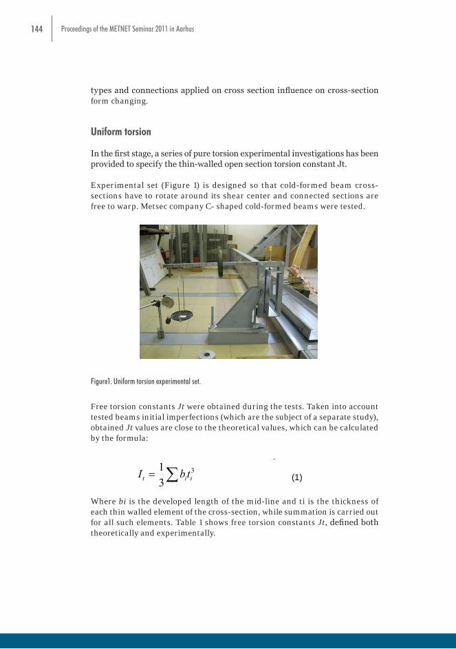
144 Proceedings of the METNET Seminar 2011 in Aarhus
types and connections applied on cross section influence on cross-section form changing.
Uniform torsion
In the first stage, a series of pure torsion experimental investigations has been provided to specify the thin-walled open section torsion constant Jt.
Experimental set (Figure 1) is designed so that cold-formed beam cross-sections have to rotate around its shear center and connected sections are free to warp. Metsec company C- shaped cold-formed beams were tested.
is carried out on the basis of a reduced cross-section, caused by local buckling of the compressed cross-section elements. Both approaches do not take into account the ability of cold-formed steel thin-walled profiles to change its cross section shape proportionally to the load acting on it. In this connection it is necessary to conduct theoretical and experimental studies of the cross-section deformation effect on behavior of cold-formed steel profiles. First of all, it is important to find out the range of section-length characteristics for cold-formed profiles in which the fact of not taking into account of contour deformation of the cross-section leads to the significant, from an engineering point of view, error in the calculations. Also it is needed to estimate how load types and connections applied on cross section influence on cross-section form changing. Uniform torsion In the first stage, a series of pure torsion experimental investigations has been provided to specify the thin-walled open section torsion constant Jt. Experimental set (Figure 2) is designed so that cold-formed beam cross-sections have to rotate around its shear center and connected sections are free to warp. Metsec company C- shaped cold-formed beams were tested.
Figure2. Uniform torsion experimental set.
Free torsion constants Jt were obtained during the tests. Taken into account tested beams initial imperfections (which are the subject of a separate study), obtained Jt values are close to the theoretical values, which can be calculated by the formula:
3
31
iit tbI (1)
Where bi is the developed length of the mid-line and ti is the thickness of each thin walled element of the cross-section, while summation is carried out for all such elements. Table 1 shows free torsion constants Jt, defined both theoretically and experimentally.
Table1. Uniform torsion experiment results.
Figure1. Uniform torsion experimental set.
Free torsion constants Jt were obtained during the tests. Taken into account tested beams initial imperfections (which are the subject of a separate study), obtained Jt values are close to the theoretical values, which can be calculated by the formula:
is carried out on the basis of a reduced cross-section, caused by local buckling of the compressed cross-section elements. Both approaches do not take into account the ability of cold-formed steel thin-walled profiles to change its cross section shape proportionally to the load acting on it. In this connection it is necessary to conduct theoretical and experimental studies of the cross-section deformation effect on behavior of cold-formed steel profiles. First of all, it is important to find out the range of section-length characteristics for cold-formed profiles in which the fact of not taking into account of contour deformation of the cross-section leads to the significant, from an engineering point of view, error in the calculations. Also it is needed to estimate how load types and connections applied on cross section influence on cross-section form changing. Uniform torsion In the first stage, a series of pure torsion experimental investigations has been provided to specify the thin-walled open section torsion constant Jt. Experimental set (Figure 2) is designed so that cold-formed beam cross-sections have to rotate around its shear center and connected sections are free to warp. Metsec company C- shaped cold-formed beams were tested.
Figure2. Uniform torsion experimental set.
Free torsion constants Jt were obtained during the tests. Taken into account tested beams initial imperfections (which are the subject of a separate study), obtained Jt values are close to the theoretical values, which can be calculated by the formula:
3
31
iit tbI (1)
Where bi is the developed length of the mid-line and ti is the thickness of each thin walled element of the cross-section, while summation is carried out for all such elements. Table 1 shows free torsion constants Jt, defined both theoretically and experimentally.
Table1. Uniform torsion experiment results.
Where bi is the developed length of the mid-line and ti is the thickness of each thin walled element of the cross-section, while summation is carried out for all such elements. Table 1 shows free torsion constants Jt, defined both theoretically and experimentally.
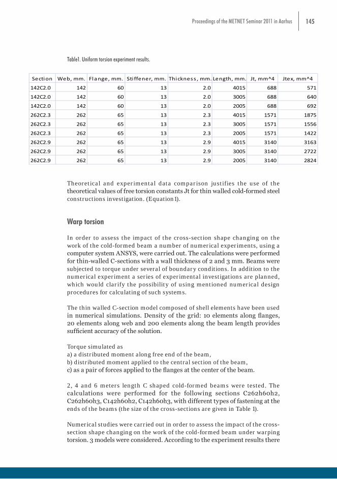
145Proceedings of the METNET Seminar 2011 in Aarhus
Table1. Uniform torsion experiment results.
Section Web, mm. Flange, mm. Sti ffener, mm. Thickness , mm. Length, mm. Jt, mm^4 Jtex, mm^4
142С2.0 142 60 13 2.0 4015 688 571
142С2.0 142 60 13 2.0 3005 688 640
142С2.0 142 60 13 2.0 2005 688 692
262С2.3 262 65 13 2.3 4015 1571 1875
262С2.3 262 65 13 2.3 3005 1571 1556
262С2.3 262 65 13 2.3 2005 1571 1422
262С2.9 262 65 13 2.9 4015 3140 3163
262С2.9 262 65 13 2.9 3005 3140 2722
262С2.9 262 65 13 2.9 2005 3140 2824
Theoretical and experimental data comparison justifies the use of the theoretical values of free torsion constants Jt for thin walled cold-formed steel constructions investigation. (Equation1).
Warp torsion
In order to assess the impact of the cross-section shape changing on the work of the cold-formed beam a number of numerical experiments, using a computer system ANSYS, were carried out. The calculations were performed for thin-walled C-sections with a wall thickness of 2 and 3 mm. Beams were subjected to torque under several of boundary conditions. In addition to the numerical experiment a series of experimental investigations are planned, which would clarify the possibility of using mentioned numerical design procedures for calculating of such systems.
The thin walled C-section model composed of shell elements have been used in numerical simulations. Density of the grid: 10 elements along flanges, 20 elements along web and 200 elements along the beam length provides sufficient accuracy of the solution.
Torque simulated as a) a distributed moment along free end of the beam, b) distributed moment applied to the central section of the beam, c) as a pair of forces applied to the flanges at the center of the beam.
2, 4 and 6 meters length C shaped cold-formed beams were tested. The calculations were performed for the following sections C262h60h2, C262h60h3, C142h60h2, C142h60h3, with different types of fastening at the ends of the beams (the size of the cross-sections are given in Table 1).
Numerical studies were carried out in order to assess the impact of the cross-section shape changing on the work of the cold-formed beam under warping torsion. 3 models were considered. According to the experiment results there
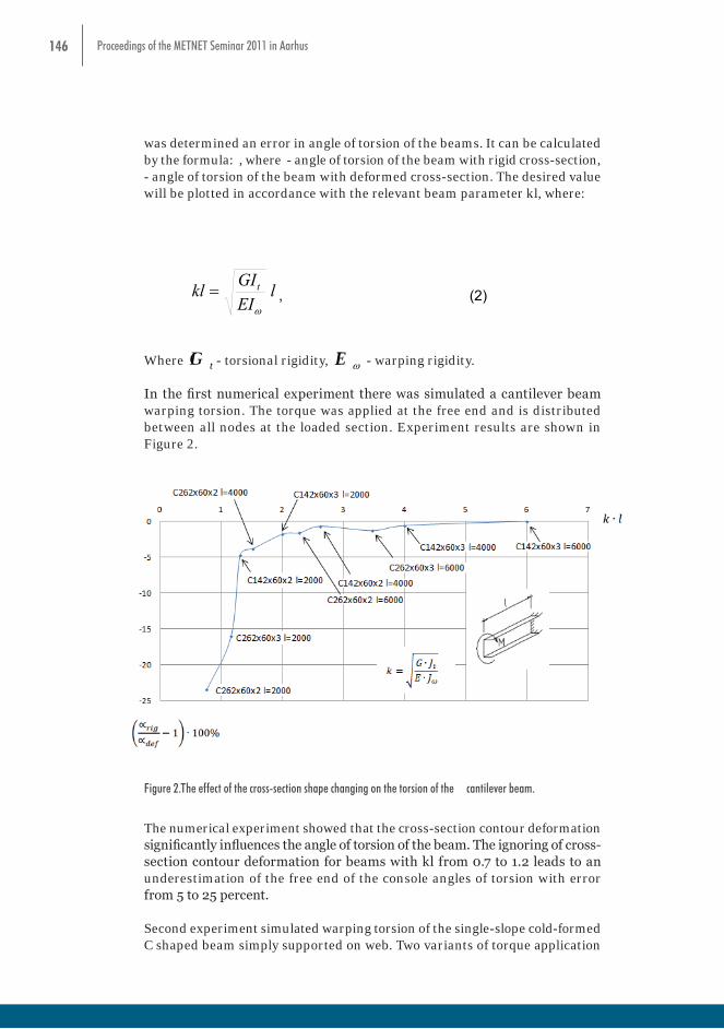
146 Proceedings of the METNET Seminar 2011 in Aarhus
was determined an error in angle of torsion of the beams. It can be calculated by the formula: , where - angle of torsion of the beam with rigid cross-section, - angle of torsion of the beam with deformed cross-section. The desired value will be plotted in accordance with the relevant beam parameter kl, where:
lEIGIkl t
, (2)
Where tGI - torsional rigidity, EI - warping rigidity. In the first numerical experiment there was simulated a cantilever beam warping torsion. The torque was applied at the free end and is distributed between all nodes at the loaded section. Experiment results are shown in Figure 3.
Figure 3.The effect of the cross-section shape changing on the torsion of the cantilever beam.
The numerical experiment showed that the cross-section contour deformation significantly influences the angle of torsion of the beam. The ignoring of cross-section contour deformation for beams with kl from 0.7 to 1.2 leads to an underestimation of the free end of the console angles of torsion with error from 5 to 25 percent. Second experiment simulated warping torsion of the single-slope cold-formed C shaped beam simply supported on web. Two variants of torque application were considered. The distributed moment applied to the middle section of the beam, and the pair of forces applied to flanges at the middle section of the beam. The experimental results are shown in Figure 4.
Where tGI - torsional rigidity, ωEI - warping rigidity.
In the first numerical experiment there was simulated a cantilever beam warping torsion. The torque was applied at the free end and is distributed between all nodes at the loaded section. Experiment results are shown in Figure 2.
lEIGIkl t
, (2)
Where tGI - torsional rigidity, EI - warping rigidity. In the first numerical experiment there was simulated a cantilever beam warping torsion. The torque was applied at the free end and is distributed between all nodes at the loaded section. Experiment results are shown in Figure 3.
Figure 3.The effect of the cross-section shape changing on the torsion of the cantilever beam.
The numerical experiment showed that the cross-section contour deformation significantly influences the angle of torsion of the beam. The ignoring of cross-section contour deformation for beams with kl from 0.7 to 1.2 leads to an underestimation of the free end of the console angles of torsion with error from 5 to 25 percent. Second experiment simulated warping torsion of the single-slope cold-formed C shaped beam simply supported on web. Two variants of torque application were considered. The distributed moment applied to the middle section of the beam, and the pair of forces applied to flanges at the middle section of the beam. The experimental results are shown in Figure 4.
Figure 2.The effect of the cross-section shape changing on the torsion of the cantilever beam.
The numerical experiment showed that the cross-section contour deformation significantly influences the angle of torsion of the beam. The ignoring of cross-section contour deformation for beams with kl from 0.7 to 1.2 leads to an underestimation of the free end of the console angles of torsion with error from 5 to 25 percent.
Second experiment simulated warping torsion of the single-slope cold-formed C shaped beam simply supported on web. Two variants of torque application
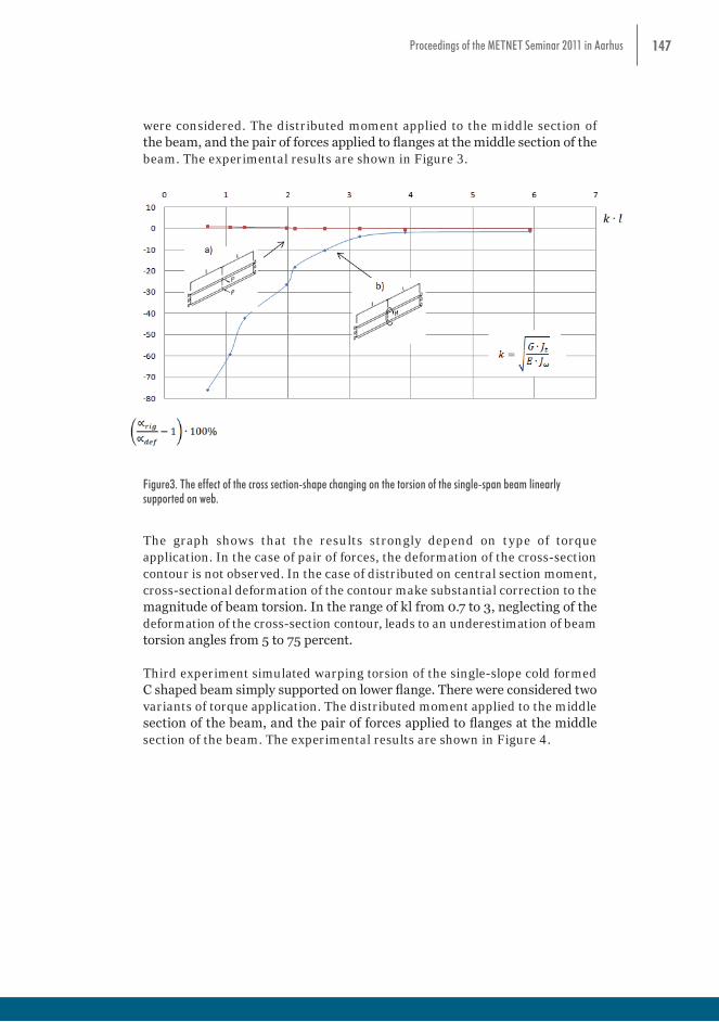
147Proceedings of the METNET Seminar 2011 in Aarhus
were considered. The distributed moment applied to the middle section of the beam, and the pair of forces applied to flanges at the middle section of the beam. The experimental results are shown in Figure 3.
Figure4. The effect of the cross section-shape changing on the torsion of the single-sloap beam linearly
supported on web. The graph shows that the results strongly depend on type of torque application. In the case of pair of forces, the deformation of the cross-section contour is not observed. In the case of distributed on central section moment, cross-sectional deformation of the contour make substantial correction to the magnitude of beam torsion. In the range of kl from 0.7 to 3, neglecting of the deformation of the cross-section contour, leads to an underestimation of beam torsion angles from 5 to 75 percent. Third experiment simulated warping torsion of the single-slope cold formed C shaped beam simply supported on lower flange. There were considered two variants of torque application. The distributed moment applied to the middle section of the beam, and the pair of forces applied to flanges at the middle section of the beam. The experimental results are shown in Figure 5.
Figure 5. The effect of the cross-section shape changing on the torsion of the of the single-sloap beam
linearly supported on lower flange.
Figure3. The effect of the cross section-shape changing on the torsion of the single-span beam linearly supported on web.
The graph shows that the results strongly depend on type of torque application. In the case of pair of forces, the deformation of the cross-section contour is not observed. In the case of distributed on central section moment, cross-sectional deformation of the contour make substantial correction to the magnitude of beam torsion. In the range of kl from 0.7 to 3, neglecting of the deformation of the cross-section contour, leads to an underestimation of beam torsion angles from 5 to 75 percent.
Third experiment simulated warping torsion of the single-slope cold formed C shaped beam simply supported on lower flange. There were considered two variants of torque application. The distributed moment applied to the middle section of the beam, and the pair of forces applied to flanges at the middle section of the beam. The experimental results are shown in Figure 4.
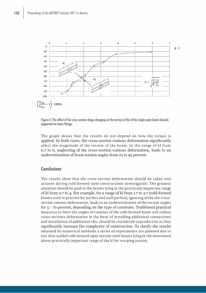
148 Proceedings of the METNET Seminar 2011 in Aarhus
Figure4. The effect of the cross section-shape changing on the torsion of the single-sloap beam linearly
supported on web. The graph shows that the results strongly depend on type of torque application. In the case of pair of forces, the deformation of the cross-section contour is not observed. In the case of distributed on central section moment, cross-sectional deformation of the contour make substantial correction to the magnitude of beam torsion. In the range of kl from 0.7 to 3, neglecting of the deformation of the cross-section contour, leads to an underestimation of beam torsion angles from 5 to 75 percent. Third experiment simulated warping torsion of the single-slope cold formed C shaped beam simply supported on lower flange. There were considered two variants of torque application. The distributed moment applied to the middle section of the beam, and the pair of forces applied to flanges at the middle section of the beam. The experimental results are shown in Figure 5.
Figure 5. The effect of the cross-section shape changing on the torsion of the of the single-sloap beam
linearly supported on lower flange. Figure 4. The effect of the cross-section shape changing on the torsion of the of the single-span beam linearly
supported on lower flange.
The graph shows that the results do not depend on how the torque is applied. In both cases, the cross-section contour deformation significantly affect the magnitude of the torsion of the beam. In the range of kl from 0.7 to 6, neglecting of the cross-section contour deformation, leads to an underestimation of beam torsion angles from 10 to 95 percent.
Conclusions
The results show that the cross-section deformation should be taken into account during cold-formed steel constructions investigation. The greatest attention should be paid to the beams lying in the practically important range of kl from 0.7 to 4. For example, for a range of kl from 1.7 to 3.7 (cold-formed beams used in practice for purlins and wall purlins), ignoring of the the cross-section contour deformation, leads to an underestimation of the torsion angles for 5 - 70 percent, depending on the type of constrain. Traditional practical measures to limit the angles of rotation of the cold-formed beam and reduce cross-sections deformation in the form of installing additional connections and installation of additional ribs, should be considered unproductive as they significantly increase the complexity of construction. To clarify the results obtained by numerical methods a series of experiments are planned due to test thin-walled cold-formed open section steel beams lying in the mentioned above practically important range of the kl for warping torsion.

149Proceedings of the METNET Seminar 2011 in Aarhus
COMMENTS ABOUT THE DESIGN OF RUNWAY GIRDERS ACCORDING TO NEW EN STANDARDS
Helmuth Köber,
Bogdan Ştefănescu
Şerban Dima
Steel Structures Department,
Technical University of Civil Engineering Bucharest, Romania
Abstract
The present paper is intended to illustrate some particular aspects in using the new European standard EN 1993-6: 2007 (Eurocode 3: Design of steel structures – Part 6: Crane supporting structures) and the other involved Eurocodes regarding the design of runway beams for travelling cranes. References are also made to the Romanian and German design regulations in this matter.
Two kind of simply supported runway girders were analyzed to show these particular aspects:
• 9 meters span girders for two overhead travelling cranes, having each a hoist load of 20 tons;
• 6 meters span girders for an underslung travelling crane, having a 5 tons hoist load.
The design results differences among the European standards and appropriate Romanian regulations regarding the design of runway beams were highlighted.
Actions induced by cranes on the runway girders
Analyzed travelling cranes
The loads produced by travelling cranes were evaluated according to EN 1991-3: 2006 (Eurocode 1: Actions on structures – Part 3: Actions induced by cranes and machinery) and according to the appropriate Romanian code [1].
Two overhead travelling storage cranes with intermittent operation were considered (hoisting class HC2; S-class S4 according to [5]). The two cranes are working together one the same runway. The hoist load is 20t, the unloaded crane weight is 9220kg, the span of the crane is 16.5m, the maximum crane travelling speed is 40m/min, the weight of the crab is 1850kg and the maximum crab travelling speed is 25m/min.
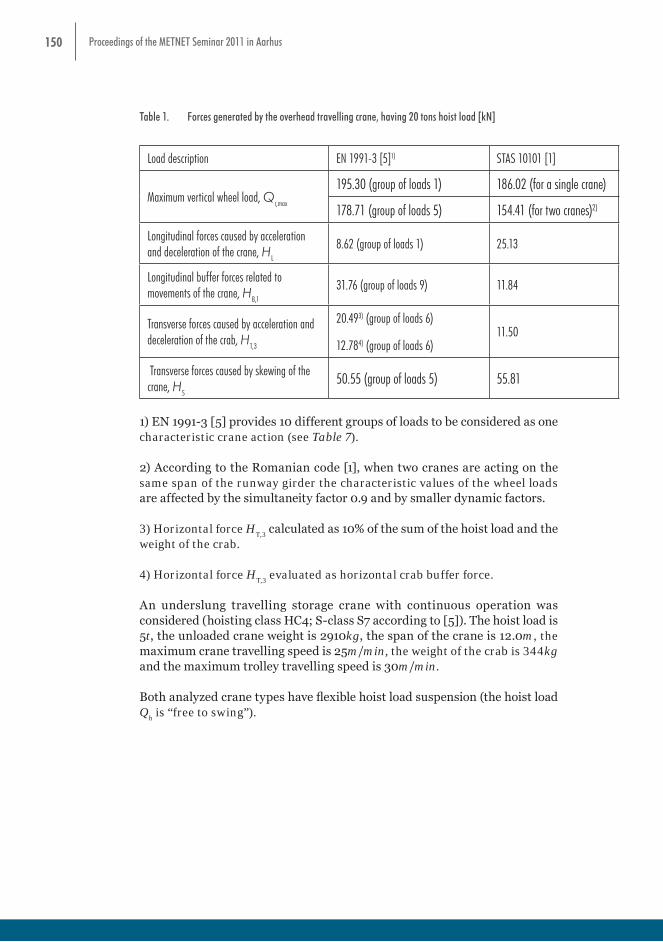
150 Proceedings of the METNET Seminar 2011 in Aarhus
Table 1. Forces generated by the overhead travelling crane, having 20 tons hoist load [kN]
Load description EN 1991-3 [5]1) STAS 10101 [1]
Maximum vertical wheel load, Qr,max
195.30 (group of loads 1) 186.02 (for a single crane)
178.71 (group of loads 5) 154.41 (for two cranes)2)
Longitudinal forces caused by acceleration and deceleration of the crane, HL
8.62 (group of loads 1) 25.13
Longitudinal buffer forces related to movements of the crane, HB,1
31.76 (group of loads 9) 11.84
Transverse forces caused by acceleration and deceleration of the crab, HT,3
20.493) (group of loads 6)
12.784) (group of loads 6)11.50
Transverse forces caused by skewing of the crane, HS
50.55 (group of loads 5) 55.81
1) EN 1991-3 [5] provides 10 different groups of loads to be considered as one characteristic crane action (see Table 7).
2) According to the Romanian code [1], when two cranes are acting on the same span of the runway girder the characteristic values of the wheel loads are affected by the simultaneity factor 0.9 and by smaller dynamic factors.
3) Horizontal force HT,3
calculated as 10% of the sum of the hoist load and the weight of the crab.
4) Horizontal force HT,3
evaluated as horizontal crab buffer force.
An underslung travelling storage crane with continuous operation was considered (hoisting class HC4; S-class S7 according to [5]). The hoist load is 5t, the unloaded crane weight is 2910kg, the span of the crane is 12.0m, the maximum crane travelling speed is 25m/min, the weight of the crab is 344kg and the maximum trolley travelling speed is 30m/min.
Both analyzed crane types have flexible hoist load suspension (the hoist load Q
h is “free to swing”).
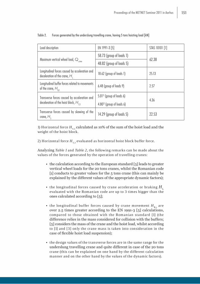
151Proceedings of the METNET Seminar 2011 in Aarhus
Table 2. Forces generated by the underslung travelling crane, having 5 tons hoisting load [kN]
Load description EN 1991-3 [5] STAS 10101 [1]
Maximum vertical wheel load, Qr,max
58.73 (group of loads 1)62.38
48.82 (group of loads 5)
Longitudinal forces caused by acceleration and deceleration of the crane, HL
18.62 (group of loads 1) 25.13
Longitudinal buffer forces related to movements of the crane, HB,1
6.48 (group of loads 9) 2.57
Transverse forces caused by acceleration and deceleration of the hoist block, HT,3
5.011) (group of loads 6)
4.802) (group of loads 6)4.36
Transverse forces caused by skewing of the crane, HS
14.29 (group of loads 5) 22.53
1) Horizontal force HT,3
calculated as 10% of the sum of the hoist load and the weight of the hoist block.
2) Horizontal force HT,3
evaluated as horizontal hoist block buffer force.
Analyzing Table 1 and Table 2, the following remarks can be made about the values of the forces generated by the operation of travelling cranes:
• the calculation according to the European standard [5] leads to greater vertical wheel loads for the 20 tons cranes, whilst the Romanian code [1] conducts to greater values for the 5 tons crane (this can mainly be explained by the different values of the appropriate dynamic factors);
• the longitudinal forces caused by crane acceleration or braking HL
evaluated with the Romanian code are up to 3 times bigger than the ones calculated according to [5];
• the longitudinal buffer forces caused by crane movement HB,1
are over 2.5 times greater according to the EN 1991-3 [5] calculations, compared to those obtained with the Romanian standard [1] (the difference relies in the mass considered for collision with the buffers; [5] considers the mass of the crane and the hoist load, whilst according to [1] and [3] only the crane mass is taken into consideration in the case of flexible hoist load suspension);
• the design values of the transverse forces are in the same range for the underslung travelling crane and quite different in case of the 20 tons crane (this can be explained on one hand by the different calculation manner and on the other hand by the values of the dynamic factors).
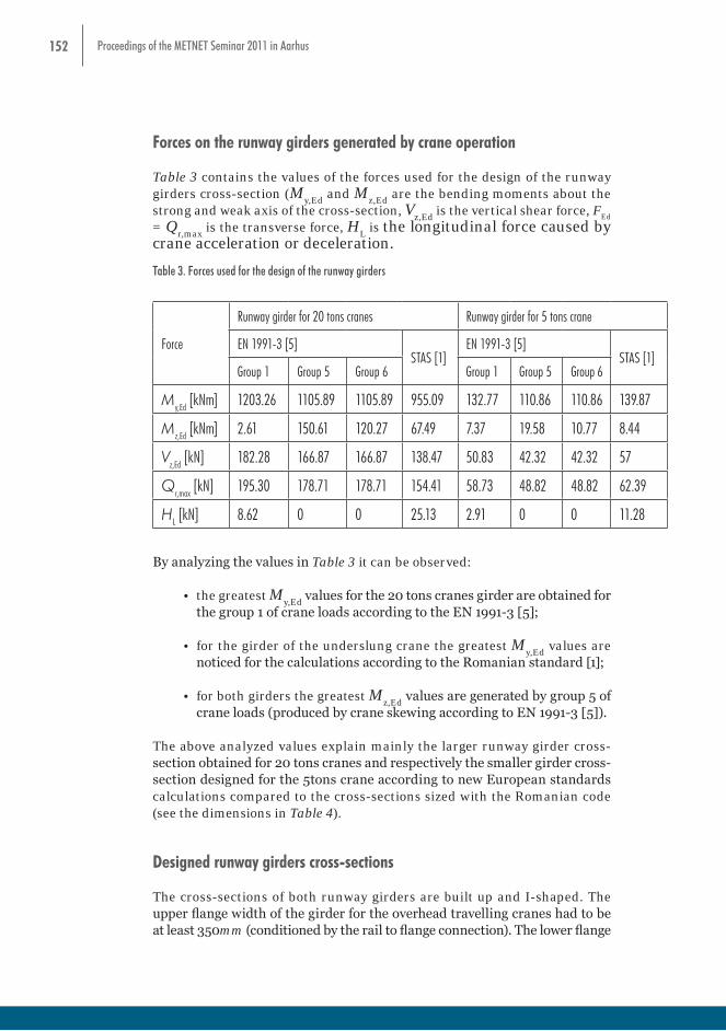
152 Proceedings of the METNET Seminar 2011 in Aarhus
Forces on the runway girders generated by crane operation
Table 3 contains the values of the forces used for the design of the runway girders cross-section (M
y,Ed and M
z,Ed are the bending moments about the
strong and weak axis of the cross-section, Vz,Ed
is the vertical shear force, FEd
= Q
r,max is the transverse force, H
L is the longitudinal force caused by
crane acceleration or deceleration.
Table 3. Forces used for the design of the runway girders
Force
Runway girder for 20 tons cranes Runway girder for 5 tons crane
EN 1991-3 [5]STAS [1]
EN 1991-3 [5]STAS [1]
Group 1 Group 5 Group 6 Group 1 Group 5 Group 6
My,Ed [kNm] 1203.26 1105.89 1105.89 955.09 132.77 110.86 110.86 139.87
Mz,Ed [kNm] 2.61 150.61 120.27 67.49 7.37 19.58 10.77 8.44
Vz,Ed [kN] 182.28 166.87 166.87 138.47 50.83 42.32 42.32 57
Qr,max [kN] 195.30 178.71 178.71 154.41 58.73 48.82 48.82 62.39
HL [kN] 8.62 0 0 25.13 2.91 0 0 11.28
By analyzing the values in Table 3 it can be observed:
• the greatest My,Ed
values for the 20 tons cranes girder are obtained for the group 1 of crane loads according to the EN 1991-3 [5];
• for the girder of the underslung crane the greatest My,Ed
values are noticed for the calculations according to the Romanian standard [1];
• for both girders the greatest Mz,Ed
values are generated by group 5 of crane loads (produced by crane skewing according to EN 1991-3 [5]).
The above analyzed values explain mainly the larger runway girder cross-section obtained for 20 tons cranes and respectively the smaller girder cross-section designed for the 5tons crane according to new European standards calculations compared to the cross-sections sized with the Romanian code (see the dimensions in Table 4).
Designed runway girders cross-sections
The cross-sections of both runway girders are built up and I-shaped. The upper flange width of the girder for the overhead travelling cranes had to be at least 350mm (conditioned by the rail to flange connection). The lower flange

153Proceedings of the METNET Seminar 2011 in Aarhus
width of the runway girder for the underslung crane had to be 150mm and was imposed by the producer of the crane.
Table 4. Runway girders cross-sections [mm]
PlateRunway girder for 20 tons cranes Runway girder for 5 tons crane
EN 1991-3 [5] STAS 10108 [2] EN 1991-3 [5] STAS 10108 [2]
Upper flange 370 x 14 350 x 14 280 x 10 300 x 10
Web 950 x 8 850 x 8 360 x 6 380 x 6
Lower flange 300 x 14 300 x 14 150 x 10 150 x 10
Both runway girders are simple supported. A surge girder was provided at the upper, compressed flange of each runway girder. The following limit states were taken into consideration for the design of the runway girders: resistance of cross-section, resistance of the web to wheel loads, resistance of bottom flanges to wheel loads, buckling of the web plate, serviceability and fatigue limit states.
The cross-sections designed according to the new European standards were checked according to the in charge Romanian codes in order to ensure an objective comparison (to avoid the influence of the different load estimation procedures) between the two sets of European and Romanian norms used for the design of runway girders. The results are presented in the tables below.
Table 5. Checking of the runway girder cross-section for the two 20 tons cranes
Group of codes used for the checks of the runway girder
Demand/Capacity ratio for
resistance for global bending
resistance of the web to wheel loads
resistance for combined bending and shear
buckling of the web plate
serviceability
limit state
fatigue
limit state
European 0.980 0.4651) 0.961 0.953 0.887 0.796
Romanian 1.047 0.580 0.934 0.868 0.931 0.395 1) The crane rail was considered not rigidly fixed to the flange of the runway girder.

154 Proceedings of the METNET Seminar 2011 in Aarhus
Table 6. Checking of the runway girder cross-section for the 5 tons crane
Group of codes used for the checks of the runway girder
Demand/Capacity ratio for
resistance for global bending
resistance of bottom flanges to wheel loads
resistance for combined bending and shear
buckling of the web plate
serviceability
limit state
fatigue
limit state
European 0.942 0.684 0.944 0.425 0.873 0.837
Romanian 1.006 0.835 0.917 0.394 0.822 0.468
Analyzing the values in Table 5 and Table 6 it can be noticed that the checks for bending resistance of the cross-section, resistance of bottom flanges to wheel loads are more severe in case of the Romanian standards, whilst the checks against buckling of the web plate and resistance of the cross-section for combined bending and shear are more severe in case of the European codes.
Comments – Remarks about actions
The European standard [5] gives several groups of loads caused by the use of travelling cranes in table 2.2 (see Table 7). The load groups 1, 5 and 6 in table 4 are the most severe when sizing the cross-section of the runway girder. The greatest value of the bending moment on the runway girder is generally obtained with group 1 of loads. For this group the self-weight of the crane Q
c
and the hoist load Qh are amplified by different dynamic factors ( 1ϕ for Q
c,
respectively 2ϕ for Qh). Most of travelling cranes producers offer only the
characteristic values for the relevant vertical wheel loads, where the influences of Q
c and Q
h are not separated. Following this, these producer’s values cannot
be used for the procedure recommended by [5].

155Proceedings of the METNET Seminar 2011 in Aarhus
Table 7. Groups of loads considered as one characteristic crane action (extracted from [5] table 2.2)
Groups of loads
Force Symbol Ultimate Limit State T e s t load
Acci-
dental
1 2 3 4 5 6 7 8 9 10
1 Self-weight of crane Qc 1ϕ 1ϕ 14ϕ 4ϕ 4ϕ 1
1ϕ 1 1
2 Hoist load Qh 2ϕ 3ϕ -4ϕ 4ϕ 4ϕ ç - 1 1
3Acceleration of crane bridge
H L , HT 5ϕ 5ϕ 5ϕ 5ϕ - - -
5ϕ - -
4Skewing of crane bridge
HS - - - - 1 - - - - -
5Acceleration or braking of crab or hoist block
HT3 - - - - - 1 - - - -
6 In-service wind FW* 1 1 1 1 1 - - 1 - -
7 Test load QT - - - - - - -6ϕ - -
8 Buffer force HB - - - - - - - -7ϕ -
9 Tilting force HTA - - - - - - - - - 1
The proper choice of the values for the dynamic factor 5ϕ according to table 2.6 from [5] could be argued. There is a lack of information for choosing a value between the limits given in that table (the limit between smoothly and sudden changes of the forces is not defined). In the previously presented examples 5ϕ was considered 1.5.
Table 8. Values of the dynamic factor φ5 (extracted from [5] table 2.6)
Dynamic factor φ5 Specific useφ5 =1.0 for centrifugal forces ≤ φ5 ≤ for systems where forces change smoothly ≤ φ5 ≤ for cases where sudden changes can occurφ5 =3.0 for drives with considerable backlash
The code [5] does not indicate an explicit procedure for calculating the horizontal force H
T,3 caused by acceleration or deceleration of the crab or
trolley. Title 2.7.5 in [5] says that the horizontal force HT,3
may be assumed to be covered by the horizontal buffer force H
B,2 (produced by the movement of
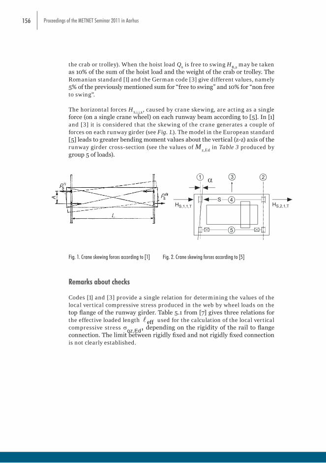
156 Proceedings of the METNET Seminar 2011 in Aarhus
the crab or trolley). When the hoist load Qh is free to swing H
B,2 may be taken
as 10% of the sum of the hoist load and the weight of the crab or trolley. The Romanian standard [1] and the German code [3] give different values, namely 5% of the previously mentioned sum for “free to swing” and 10% for “non free to swing”.
The horizontal forces HS,i,j,k
, caused by crane skewing, are acting as a single force (on a single crane wheel) on each runway beam according to [5]. In [1] and [3] it is considered that the skewing of the crane generates a couple of forces on each runway girder (see Fig. 1.). The model in the European standard [5] leads to greater bending moment values about the vertical (z-z) axis of the runway girder cross-section (see the values of M
z,Ed in Table 3 produced by
group 5 of loads).
The code [5] does not indicate an explicit procedure for calculating the horizontal force HT,3 caused by acceleration or deceleration of the crab or trolley. Title 2.7.5 in [5] says that the horizontal force HT,3 may be assumed to be covered by the horizontal buffer force HB,2 (produced by the movement of the crab or trolley). When the hoist load Qh is free to swing HB,2 may be taken as 10% of the sum of the hoist load and the weight of the crab or trolley. The Romanian standard [1] and the German code [3] give different values, namely 5% of the previously mentioned sum for “free to swing” and 10% for “non free to swing”. The horizontal forces HS,i,j,k, caused by crane skewing, are acting as a single force (on a single crane wheel) on each runway beam according to [5]. In [1] and [3] it is considered that the skewing of the crane generates a couple of forces on each runway girder (see Fig. 1.). The model in the European standard [5] leads to greater bending moment values about the vertical (z-z) axis of the runway girder cross-section (see the values of Mz,Ed in Table 3 produced by group 5 of loads).
Fig. 1. Crane skewing forces according to [1] Fig. 2. Crane skewing forces according to [5]
Remarks about checks Codes [1] and [3] provide a single relation for determining the values of the local vertical compressive stress produced in the web by wheel loads on the top flange of the runway girder. Table 5.1 from [7] gives three relations for the effective loaded length eff used for the calculation of the local vertical compressive stress oz,Ed, depending on the rigidity of the rail to flange connection. The limit between rigidly fixed and not rigidly fixed connection is not clearly established.
Table 7. Values of the local vertical compressive stress oz,Ed
Situation Effective loaded length formula eff eff [mm] oz,Ed [N/mm2]Crane rail rigidly fixed to the flange 3
1wrfeff ]/[3,25 tI 289.25 84.40
Crane rail not rigidly fixed to flange
31
wefff,reff ]/)[(3,25 tII 223.31 109.32
Crane rail mounted on a suitable resilient elastomeric bearing pad at least 6mm thick.
31
wefff,reff ]/)[(4,25 tII 292.03 83.60
Calculation according to the German [3] and Romanian codes 198.00 101.26
HS,1,1,T
1 23
4
5
HS,2,1,TS
Fig. 1. Crane skewing forces according to [1] Fig. 2. Crane skewing forces according to [5]
Remarks about checks
Codes [1] and [3] provide a single relation for determining the values of the local vertical compressive stress produced in the web by wheel loads on the top flange of the runway girder. Table 5.1 from [7] gives three relations for the effective loaded length eff used for the calculation of the local vertical compressive stress soz,Ed, depending on the rigidity of the rail to flange connection. The limit between rigidly fixed and not rigidly fixed connection is not clearly established.

157Proceedings of the METNET Seminar 2011 in Aarhus
Table 7. Values of the local vertical compressive stress soz,Ed
Situation Effective loaded length formula eff eff [mm] soz,Ed [N/mm2]
Crane rail rigidly fixed to the flange 3
1wrfeff ]/[3,25 tI=
289.25 84.40
Crane rail not rigidly fixed to flange 3
1wefff,reff ]/)[(3,25 tII +=
223.31 109.32
Crane rail mounted on a suitable resilient elastomeric bearing pad at least 6mm thick.
31
wefff,reff ]/)[(4,25 tII +=292.03 83.60
Calculation according to the German [3] and Romanian codes [1] 198.00 101.26
The fatigue check requires the use of the partial safety factor γMf
given in table 3.1 of [8], depending on concepts like “low and high failure consequence”, “damage tolerant” and “safe life”, which are not clearly defined and delimited.
A frequent loading state of the webs of runway beams is when they are simultaneously subjected to bending moment (M
y,Ed), shear force (V
z,Ed)
and transversal force (FEd
). Codes [6] and [7] do not specify an interaction checking relation for this loading state and they do not make any reference to such a relation. The Romanian code [1] provides such an interaction relation (see the last row of Table 8).
Table 8. Local buckling checks of the web for the 20 tons travelling cranes runway girders
Standard Forces Local buckling checking relation
EN 1993-1-5 My,Ed 019801 ..ã/fW
Mç
MOyy
yEd <=⋅
=; (relation 4.14 from [6])
EN 1993-1-5 Vz,Ed 0130703 ..VV
VVVç
Rd,bfRd,bw
zEd
Rd,b
zEd <=+
==
; (relation 5.10 from [6])
EN 1993-1-5 FEd 0146502 ..FFç
Rd
Ed <==; (relation 6.14 from [6])
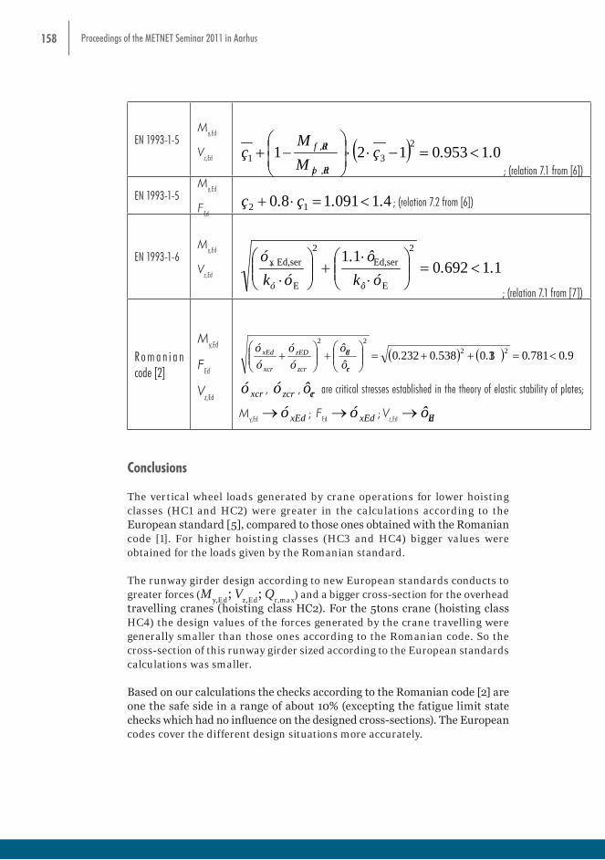
158 Proceedings of the METNET Seminar 2011 in Aarhus
EN 1993-1-5My,Ed
Vz,Ed ( ) 0195301212
31 ..çMM
çRd,pl
Rd,f <=-⋅⋅
-+
; (relation 7.1 from [6])
EN 1993-1-5My,Ed
FEd 41091180 12 ..ç.ç <=⋅+ ; (relation 7.2 from [6])
EN 1993-1-6My,Ed
Vz,Ed116920
11 2
E
Ed,ser2
E
Ed,serx, ..ók
ô.ók
ó
ôó
<=
⋅
⋅+
⋅
; (relation 7.1 from [7])
R o m a n i a n code [2]
My,Ed
FEd
Vz,Ed
( ) ( ) 90781013053802320 2222
.....ôô
óó
óó
cr
Ed
zcr
zED
xcr
xEd <=++=
+
+
xcró , zcró , crô are critical stresses established in the theory of elastic stability of plates;
My,Ed xEdó→ ; FEd xEdó→ ; Vz,Ed Edô→
Conclusions
The vertical wheel loads generated by crane operations for lower hoisting classes (HC1 and HC2) were greater in the calculations according to the European standard [5], compared to those ones obtained with the Romanian code [1]. For higher hoisting classes (HC3 and HC4) bigger values were obtained for the loads given by the Romanian standard.
The runway girder design according to new European standards conducts to greater forces (M
y,Ed; V
z,Ed; Q
r,max) and a bigger cross-section for the overhead
travelling cranes (hoisting class HC2). For the 5tons crane (hoisting class HC4) the design values of the forces generated by the crane travelling were generally smaller than those ones according to the Romanian code. So the cross-section of this runway girder sized according to the European standards calculations was smaller.
Based on our calculations the checks according to the Romanian code [2] are one the safe side in a range of about 10% (excepting the fatigue limit state checks which had no influence on the designed cross-sections). The European codes cover the different design situations more accurately.

159Proceedings of the METNET Seminar 2011 in Aarhus
References
STAS 10101/2A2-78, Actions due to the exploitation process, Loads due to travelling cranes, 1978.
STAS 10108/0-78, Non Industrial, Industrial and Agriculture Buildings, Design of steel members, 1978.
DIN 4132 Crane runways; steel structures; design and construction principles, 1981.
Eurocode 3, EN 1993-1-1: Design of steel structures - Part 1-1: General rules and rules for buildings, 2005.
Eurocode 1, EN 1991-3: Actions on structures, Part 3: Actions induced by cranes and machinery, 2006.
Eurocode 3, EN 1993-1-5: Design of steel structures - Part 1-5: Plated structural elements, 2006.
Eurocode 3, EN 1993-1-6: Design of steel structures - Part 1-6: Crane supporting structures, 2006.
Eurocode 3, EN 1993-1-9: Design of steel structures - Part 1-9: Fatigue, 2006.
160 Proceedings of the METNET Seminar 2011 in Aarhus
ANALYSIS SUPERCRITICAL BEHAVIOR OF ROD SYSTEMS
Tusnin Alexander
Tusnina Olga
Moscow State University of Civil Engineering (MSUCE), Moscow, Russia
Abstract
Behavior of designs after buckling is need to be analyzed. In this paper supercritical behavior of rod systems was studied. Numerical methods used in popular computing programs to analyze designs after buckling were considered and new methodology was proposed, which successfully used in program STK.
Introduction
In constructions there are used systems, in which abrupt changing of the shape occurs under certain load level. Acting of critical load at such systems leads to buckling, which is accompanied by huge displacements of nodes and their hops to the new equilibrium position. The value of displacements, when buckling take place, is very high and even can be comparable with length of rod. Rod designs with compressed elements can be a simple example of such systems. The Mises truss is a famous example of systems with “hops”. Modern computing programs allow performing numerical buckling analysis of these designs. Analysis perform or linear by undeformable scheme, or with account of nonlinearity, in this case during analysis with increasing of load changing of form and appearing of internal forces at construction is taken into account. At first case of analysis forces, occurring in the rods by loading the construction, are not considered, and at the second case analysis is carried out until system is not geometrically changing, which occurs at some step of load applying. The second method of analysis is more exact reflect behavior of construction before buckling, but not allow to identify supercritical behavior of construction (behavior after buckling). In some cases analysis of supercritical behavior is necessary for systems, in which load bearing capacity of whole structure remains when buckling of particular rods or parts of construction occurs. In some computing programs special rod elements are used, which allow to analyze systems with “hops”. Numerical methodology, which allows to analyze supercritical behavior of thin-walled structures, was proposed at the department of metal structures of Moscow State University of Civil Engineering. This methodology are used in computing program STK.
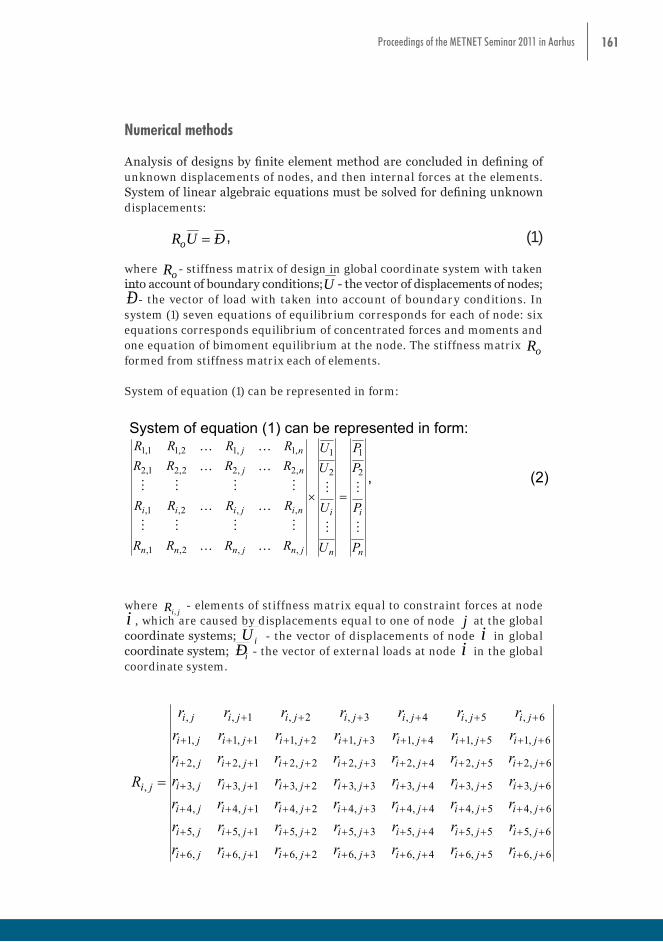
161Proceedings of the METNET Seminar 2011 in Aarhus
Numerical methods
Analysis of designs by finite element method are concluded in defining of unknown displacements of nodes, and then internal forces at the elements. System of linear algebraic equations must be solved for defining unknown displacements:
ÐURo = , (1) where oR - stiffness matrix of design in global coordinate system with taken into account of boundary conditions;U - the vector of displacements of nodes; Ð- the vector of load with taken into account of boundary conditions. In system (1) seven equations of equilibrium corresponds for each of node: six equations corresponds equilibrium of concentrated forces and moments and one equation of bimoment equilibrium at the node. The stiffness matrix oR formed from stiffness matrix each of elements.
System of equation (1) can be represented in form:
РURo , (1)
where oR - stiffness matrix of design in global coordinate system with taken into
account of boundary conditions;U - the vector of displacements of nodes; Р- the vector of load with taken into account of boundary conditions. In system (1) seven equations of equilibrium corresponds for each of node: six equations corresponds equilibrium of concentrated forces and moments and one equation of bimoment equilibrium at the node. The stiffness matrix oR formed from stiffness matrix each of elements. System of equation (1) can be represented in form:
n
i
n
i
jnjnnn
nijiii
nj
nj
P
P
PP
U
U
UU
RRRR
RRRR
RRRRRRRR
2
1
2
1
,,2,1,
,,2,1,
,2,22,21,2
,1,12,11,1
, (2)
where
jiR , - elements of stiffness matrix equal to constraint forces at node i , which
are caused by displacements equal to one of node j at the global coordinate systems; iU - the vector of displacements of node i in global coordinate system; iР - the vector of external loads at node i in the global coordinate system.
6,65,64,63,62,61,6,6
6,55,54,53,52,51,5,5
6,45,44,43,42,41,4,4
6,35,34,33,32,31,3,3
6,25,24,23,22,21,2,2
6,15,14,13,12,11,1,1
6,5,4,3,2,1,,
,
jijijijijijiji
jijijijijijiji
jijijijijijiji
jijijijijijiji
jijijijijijiji
jijijijijijiji
jijijijijijiji
ji
rrrrrrrrrrrrrrrrrrrrrrrrrrrrrrrrrrrrrrrrrrrrrrrrr
R, (3)
Herewith:
i
i
i
i
i
i
i
i
wvu
U
, (4)
i
zi
yi
xi
zi
yi
xi
i
BMMMFFF
Р , (5)
where jiR , - elements of stiffness matrix equal to constraint forces at node
i , which are caused by displacements equal to one of node j at the global coordinate systems; iU - the vector of displacements of node i in global coordinate system; iÐ - the vector of external loads at node i in the global coordinate system.
РURo , (1)
where oR - stiffness matrix of design in global coordinate system with taken into
account of boundary conditions;U - the vector of displacements of nodes; Р- the vector of load with taken into account of boundary conditions. In system (1) seven equations of equilibrium corresponds for each of node: six equations corresponds equilibrium of concentrated forces and moments and one equation of bimoment equilibrium at the node. The stiffness matrix oR formed from stiffness matrix each of elements. System of equation (1) can be represented in form:
n
i
n
i
jnjnnn
nijiii
nj
nj
P
P
PP
U
U
UU
RRRR
RRRR
RRRRRRRR
2
1
2
1
,,2,1,
,,2,1,
,2,22,21,2
,1,12,11,1
, (2)
where
jiR , - elements of stiffness matrix equal to constraint forces at node i , which
are caused by displacements equal to one of node j at the global coordinate systems; iU - the vector of displacements of node i in global coordinate system; iР - the vector of external loads at node i in the global coordinate system.
6,65,64,63,62,61,6,6
6,55,54,53,52,51,5,5
6,45,44,43,42,41,4,4
6,35,34,33,32,31,3,3
6,25,24,23,22,21,2,2
6,15,14,13,12,11,1,1
6,5,4,3,2,1,,
,
jijijijijijiji
jijijijijijiji
jijijijijijiji
jijijijijijiji
jijijijijijiji
jijijijijijiji
jijijijijijiji
ji
rrrrrrrrrrrrrrrrrrrrrrrrrrrrrrrrrrrrrrrrrrrrrrrrr
R, (3)
Herewith:
i
i
i
i
i
i
i
i
wvu
U
, (4)
i
zi
yi
xi
zi
yi
xi
i
BMMMFFF
Р , (5)
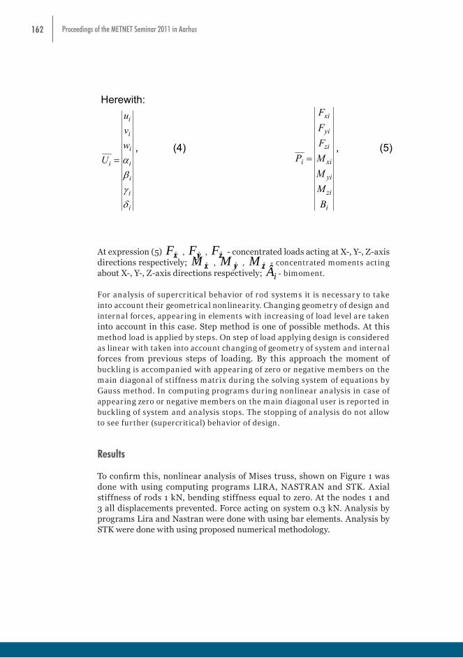
162 Proceedings of the METNET Seminar 2011 in Aarhus
РURo , (1)
where oR - stiffness matrix of design in global coordinate system with taken into
account of boundary conditions;U - the vector of displacements of nodes; Р- the vector of load with taken into account of boundary conditions. In system (1) seven equations of equilibrium corresponds for each of node: six equations corresponds equilibrium of concentrated forces and moments and one equation of bimoment equilibrium at the node. The stiffness matrix oR formed from stiffness matrix each of elements. System of equation (1) can be represented in form:
n
i
n
i
jnjnnn
nijiii
nj
nj
P
P
PP
U
U
UU
RRRR
RRRR
RRRRRRRR
2
1
2
1
,,2,1,
,,2,1,
,2,22,21,2
,1,12,11,1
, (2)
where
jiR , - elements of stiffness matrix equal to constraint forces at node i , which
are caused by displacements equal to one of node j at the global coordinate systems; iU - the vector of displacements of node i in global coordinate system; iР - the vector of external loads at node i in the global coordinate system.
6,65,64,63,62,61,6,6
6,55,54,53,52,51,5,5
6,45,44,43,42,41,4,4
6,35,34,33,32,31,3,3
6,25,24,23,22,21,2,2
6,15,14,13,12,11,1,1
6,5,4,3,2,1,,
,
jijijijijijiji
jijijijijijiji
jijijijijijiji
jijijijijijiji
jijijijijijiji
jijijijijijiji
jijijijijijiji
ji
rrrrrrrrrrrrrrrrrrrrrrrrrrrrrrrrrrrrrrrrrrrrrrrrr
R, (3)
Herewith:
i
i
i
i
i
i
i
i
wvu
U
, (4)
i
zi
yi
xi
zi
yi
xi
i
BMMMFFF
Р , (5)
At expression (5) xiF , yiF , ziF - concentrated loads acting at X-, Y-, Z-axis directions respectively; xiM , yiM , ziM - concentrated moments acting about X-, Y-, Z-axis directions respectively; i - bimoment.
For analysis of supercritical behavior of rod systems it is necessary to take into account their geometrical nonlinearity. Changing geometry of design and internal forces, appearing in elements with increasing of load level are taken into account in this case. Step method is one of possible methods. At this method load is applied by steps. On step of load applying design is considered as linear with taken into account changing of geometry of system and internal forces from previous steps of loading. By this approach the moment of buckling is accompanied with appearing of zero or negative members on the main diagonal of stiffness matrix during the solving system of equations by Gauss method. In computing programs during nonlinear analysis in case of appearing zero or negative members on the main diagonal user is reported in buckling of system and analysis stops. The stopping of analysis do not allow to see further (supercritical) behavior of design.
Results
To confirm this, nonlinear analysis of Mises truss, shown on Figure 1 was done with using computing programs LIRA, NASTRAN and STK. Axial stiffness of rods 1 kN, bending stiffness equal to zero. At the nodes 1 and 3 all displacements prevented. Force acting on system 0.3 kN. Analysis by programs Lira and Nastran were done with using bar elements. Analysis by STK were done with using proposed numerical methodology.
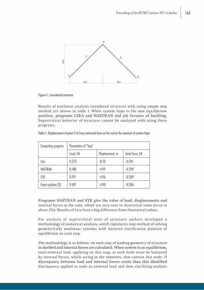
163Proceedings of the METNET Seminar 2011 in Aarhus
At expression (5) xiF , yiF , ziF - concentrated loads acting at X-, Y-, Z-axis directions
respectively; xiM , yiM , ziM - concentrated moments acting about X-, Y-, Z-axis
directions respectively; iВ - bimoment. For analysis of supercritical behavior of rod systems it is necessary to take into account their geometrical nonlinearity. Changing geometry of design and internal forces, appearing in elements with increasing of load level are taken into account in this case. Step method is one of possible methods. At this method load is applied by steps. On step of load applying design is considered as linear with taken into account changing of geometry of system and internal forces from previous steps of loading. By this approach the moment of buckling is accompanied with appearing of zero or negative members on the main diagonal of stiffness matrix during the solving system of equations by Gauss method. In computing programs during nonlinear analysis in case of appearing zero or negative members on the main diagonal user is reported in buckling of system and analysis stops. The stopping of analysis do not allow to see further (supercritical) behavior of design.
Results
To confirm this, nonlinear analysis of Mises truss, shown on Figure 1 was done with using computing programs LIRA, NASTRAN and STK. Axial stiffness of rods 1 kN, bending stiffness equal to zero. At the nodes 1 and 3 all displacements prevented. Force acting on system 0.3 kN. Analysis by programs Lira and Nastran were done with using bar elements. Analysis by STK were done with using proposed numerical methodology.
10 ì
10 ì 10 ì
1
2
3
1 2
Figure 1. Considered structure
Results of nonlinear analysis considered structure with using simple step method are shown in table 1. When system hops to the new equilibrium position, programs LIRA and NASTRAN end job because of buckling. Supercritical behavior of structure cannot be analyzed with using these programs. Table 1. Displacement of point 2 of truss and axial force at the rod at the moment of system hops
Computing
program Parameters of “hop”
Load, kN Displacement, m Axial force, kN Lira 0.273 -8.70 -0.341
Figure 1. Considered structure
Results of nonlinear analysis considered structure with using simple step method are shown in table 1. When system hops to the new equilibrium position, programs LIRA and NASTRAN end job because of buckling. Supercritical behavior of structure cannot be analyzed with using these programs.
Table 1. Displacement of point 2 of truss and axial force at the rod at the moment of system hops
Computing program Parameters of “hop”
Load, kN Displacement, m Axial force, kN
Lira 0.273 -8.70 -0.341
NASTRAN 0.188 -4.99 -0.209
STK 0.191 -4.96 -0.209
Exact solution [2] 0.187 -4.90 -0.206
Programs NASTRAN and STK give the value of load, displacements and internal forces at the rods, which are very near to theoretical value (error is about 2%). Results of Lira have a big difference from theoretical values.
For analysis of supercritical state of structure authors developed a methodology of numerical analysis, which represents step method of solving geometrically nonlinear systems with iterative clarification position of equilibrium on each step.
The methodology is as follows: on each step of loading geometry of structure is clarified and internal forces are calculated. When system is an equilibrium, total external load, applying on this step, at each node must be balanced by internal forces, which acting in the elements, that contain this node. If discrepancy between load and internal forces exists then this identified discrepancy applied to node as external load and then clarifying analysis

164 Proceedings of the METNET Seminar 2011 in Aarhus
of structure (iteration) would done. System of linear algebraic equations (1) during iteration analysis looks as:
NASTRAN 0.188 -4.99 -0.209 STK 0.191 -4.96 -0.209
Exact solution [2] 0.187 -4.90 -0.206
Programs NASTRAN and STK give the value of load, displacements and internal forces at the rods, which are very near to theoretical value (error is about 2%). Results of Lira have a big difference from theoretical values. For analysis of supercritical state of structure authors developed a methodology of numerical analysis, which represents step method of solving geometrically nonlinear systems with iterative clarification position of equilibrium on each step. The methodology is as follows: on each step of loading geometry of structure is clarified and internal forces are calculated. When system is an equilibrium, total external load, applying on this step, at each node must be balanced by internal forces, which acting in the elements, that contain this node. If discrepancy between load and internal forces exists then this identified discrepancy applied to node as external load and then clarifying analysis of structure (iteration) would done. System of linear algebraic equations (1) during iteration analysis looks as:
jijiji РUR ,,1, , (6)
where 1, jiR - the stiffness matrix on i – step of loading after j-1 – iterations, jiU , - the increment of displacements of nodes on i - step loading after j – iterations, 1, jiР - the discrepancy between total node load and internal forces on i – step of loading after j-1 – iterations. The number of iterations on each step is given before beginning the analysis. Instead of number of iterations the value of discrepancy, as a criteria of ending iterative analysis, can be given. Analysis on each step will be done until discrepancy is not bigger than specified one.
Using of this methodology (which is realized in computing program STK) allow to analyze supercritical behavior of design after buckling. For estimation proposed numerical methodology it was done analysis of Mises truss (Figure 1) with using computing programs NASTRAN and STK. At Figure 2 and 3 it are shown dependences between displacements of point 2 (Figure 1) and external load and between axial force at rod and external load, which obtained by program NASTRAN. At Figure 4 and 5 the same, obtained by STK.
where 1, -jiR - the stiffness matrix on i – step of loading after j-1 – iterations,
jiU ,∆ - the increment of displacements of nodes on i - step loading after j – iterations, 1, -∆ jiÐ - the discrepancy between total node load and internal forces on i – step of loading after j-1 – iterations. The number of iterations on each step is given before beginning the analysis. Instead of number of iterations the value of discrepancy, as a criteria of ending iterative analysis, can be given. Analysis on each step will be done until discrepancy is not bigger than specified one.
Using of this methodology (which is realized in computing program STK) allow to analyze supercritical behavior of design after buckling. For estimation proposed numerical methodology it was done analysis of Mises truss (Figure 1) with using computing programs NASTRAN and STK. At Figure 2 and 3 it are shown dependences between displacements of point 2 (Figure 1) and external load and between axial force at rod and external load, which obtained by program NASTRAN. At Figure 4 and 5 the same, obtained by STK.
Figure 2. Displacements of point 2. NASTRAN.
Figure 3. Axial forces at rod. NASTRAN.
Figure 2. Displacements of point 2. NASTRAN.
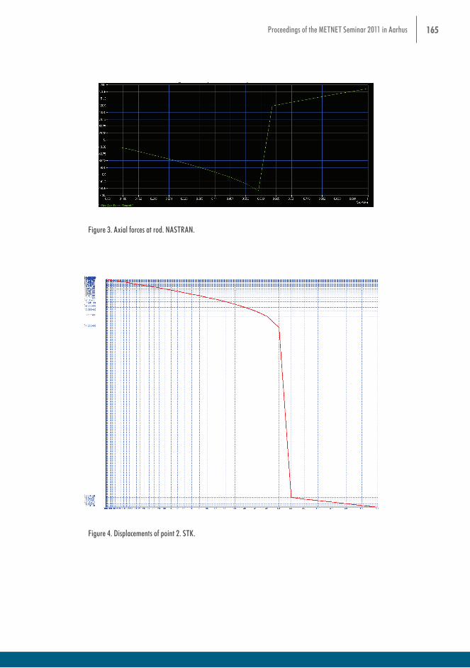
165Proceedings of the METNET Seminar 2011 in Aarhus
of structure (iteration) would done. System of linear algebraic equations (1) during iteration analysis looks as:
NASTRAN 0.188 -4.99 -0.209 STK 0.191 -4.96 -0.209
Exact solution [2] 0.187 -4.90 -0.206
Programs NASTRAN and STK give the value of load, displacements and internal forces at the rods, which are very near to theoretical value (error is about 2%). Results of Lira have a big difference from theoretical values. For analysis of supercritical state of structure authors developed a methodology of numerical analysis, which represents step method of solving geometrically nonlinear systems with iterative clarification position of equilibrium on each step. The methodology is as follows: on each step of loading geometry of structure is clarified and internal forces are calculated. When system is an equilibrium, total external load, applying on this step, at each node must be balanced by internal forces, which acting in the elements, that contain this node. If discrepancy between load and internal forces exists then this identified discrepancy applied to node as external load and then clarifying analysis of structure (iteration) would done. System of linear algebraic equations (1) during iteration analysis looks as:
jijiji РUR ,,1, , (6)
where 1, jiR - the stiffness matrix on i – step of loading after j-1 – iterations, jiU , - the increment of displacements of nodes on i - step loading after j – iterations, 1, jiР - the discrepancy between total node load and internal forces on i – step of loading after j-1 – iterations. The number of iterations on each step is given before beginning the analysis. Instead of number of iterations the value of discrepancy, as a criteria of ending iterative analysis, can be given. Analysis on each step will be done until discrepancy is not bigger than specified one.
Using of this methodology (which is realized in computing program STK) allow to analyze supercritical behavior of design after buckling. For estimation proposed numerical methodology it was done analysis of Mises truss (Figure 1) with using computing programs NASTRAN and STK. At Figure 2 and 3 it are shown dependences between displacements of point 2 (Figure 1) and external load and between axial force at rod and external load, which obtained by program NASTRAN. At Figure 4 and 5 the same, obtained by STK.
where - the stiffness matrix on i – step of loading after j-1 – iterations, - the increment of displacements of nodes on i - step loading after j
– iterations, - the discrepancy between total node load and internal forces on i – step of loading after j-1 – iterations. The number of iterations on each step is given before beginning the analysis. Instead of number of iterations the value of discrepancy, as a criteria of ending iterative analysis, can be given. Analysis on each step will be done until discrepancy is not bigger than specified one.
Using of this methodology (which is realized in computing program STK) allow to analyze supercritical behavior of design after buckling. For estimation proposed numerical methodology it was done analysis of Mises truss (Figure 1) with using computing programs NASTRAN and STK. At Figure 2 and 3 it are shown dependences between displacements of point 2 (Figure 1) and external load and between axial force at rod and external load, which obtained by program NASTRAN. At Figure 4 and 5 the same, obtained by STK.
Figure 2. Displacements of point 2. NASTRAN.
Figure 2. Displacements of point 2. NASTRAN.
Figure 3. Axial forces at rod. NASTRAN.
Figure 3. Axial forces at rod. NASTRAN.
Figure 4. Displacements of point 2. STK.
Figure 4. Displacements of point 2. STK.

166 Proceedings of the METNET Seminar 2011 in Aarhus
Figure 5. Axial forces at rods. STK.
Rod finite element SPRING was used at program NASTRAN to investigate supercritical behavior of structure. Algorithm incorporated in program was used for solving nonlinear problem. At program STK bar finite element common type was used. Load was divided at 50 uneven steps (share of load on step was calculated with using recommendations [1]), 10 iterations were done on each step. Table 2. Displacement of point 2 of truss and axial force at rods with respect supercritical behavior of
structure Computing program
Load, kN Displacement of point 2
Axial force
m % kN % NASTRAN 0.3 -23.48 99.6 0.187 97.4
STK 0.3 -23.48 99.6 0.187 97.4 Exact solution [2] 0.3 -23.57 100 0.192 100
Possibility of using developed methodology for analysis of supercritical behavior compressed elements was considered. Analysis was done for straight stand with hinged-fixed bottom end and hinged movable top end. Axial stiffness of rod
EA 100000 kN, bending stiffness EI 500 kN·m2. Compressed load N was applied to the top end. Compressive force was applied to the upper end. All calculations were
Figure 5. Axial forces at rods. STK.
Rod finite element SPRING was used at program NASTRAN to investigate supercritical behavior of structure. Algorithm incorporated in program was used for solving nonlinear problem. At program STK bar finite element common type was used. Load was divided at 50 uneven steps (share of load on step was calculated with using recommendations [1]), 10 iterations were done on each step.
Table 2. Displacement of point 2 of truss and axial force at rods with respect supercritical behavior of structure
Computing program Load, kN Displacement of point 2 Axial force
m % kN %
NASTRAN 0.3 -23.48 99.6 0.187 97.4
STK 0.3 -23.48 99.6 0.187 97.4
Exact solution [2] 0.3 -23.57 100 0.192 100

167Proceedings of the METNET Seminar 2011 in Aarhus
Possibility of using developed methodology for analysis of supercritical behavior compressed elements was considered. Analysis was done for straight stand with hinged-fixed bottom end and hinged movable top end. Axial stiffness of rod =EA 100000 kN, bending stiffness =EI 500 kN∙m2. Compressed load N was applied to the top end. Compressive force was applied to the upper end. All calculations were performed in the elastic stage of the counter material. For this simple structure critical load can be exact calculated with using Euler equation: 2
2
lEINcr
π= =49.35 kN.
Maximum value of load 100 kN was selected with respect of theoretical value of critical load. At numerical analysis for output rod of the equilibrium small shear force (maximum value is 0.1 kN) was applied to the middle of rod. Shear force changed proportionally to applied axial load on each step of loading. Nonlinearity of system was solved by step method. External load was applied at 100 equal steps, at each step of loading 20 iterations were done. Along the length rod was divided on 10 equal elements. Calculation model is shown on Figure 6. Deformed view of rod (at the same scale as calculation model) when full load is acting is shown by red color
performed in the elastic stage of the counter material. For this simple structure critical
load can be exact calculated with using Euler equation: 2
2
lEINcr
=49.35 kN.
Maximum value of load 100 kN was selected with respect of theoretical value of critical load. At numerical analysis for output rod of the equilibrium small shear force (maximum value is 0.1 kN) was applied to the middle of rod. Shear force changed proportionally to applied axial load on each step of loading. Nonlinearity of system was solved by step method. External load was applied at 100 equal steps, at each step of loading 20 iterations were done. Along the length rod was divided on 10 equal elements. Calculation model is shown on Figure 6. Deformed view of rod (at the same scale as calculation model) when full load is acting is shown by red color
Figure 6. Calculation model and its deformed view.
Results of numerical analysis were compared with analytical values of displacements at the middle of rod after buckling. Analytically displacements were obtained with using known methodology [3]. Displacement of the middle of rod after buckling is determined by solution of equation:
Figure 6. Calculation model and its deformed view.
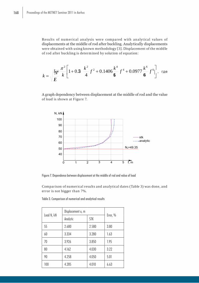
168 Proceedings of the METNET Seminar 2011 in Aarhus
Results of numerical analysis were compared with analytical values of displacements at the middle of rod after buckling. Analytically displacements were obtained with using known methodology [3]. Displacement of the middle of rod after buckling is determined by solution of equation:
+++= 6
64
42
22
640977.0
161406.0
425.01 fkfkfk
kl π
, где
EINk =
A graph dependency between displacement at the middle of rod and the value of load is shown at Figure 7.
6
64
42
22
640977.0
161406.0
425.01 fkfkfk
kl , где
EINk
A graph dependency between displacement at the middle of rod and the value of load is shown at Figure 7.
Figure 7. Dependence between displacement at the middle of rod and value of load
Comparison of numerical results and analytical dates (Table 3) was done, and error is not bigger than 7%.
Table 3. Comparison of numerical and analytical results
Load N, kN Displacement u, m Error, % Analytic STK 55 2.680 2.580 3.80 60 3.334 3.280 1.63 70 3.926 3.850 1.95 80 4.162 4.030 3.22 90 4.258 4.050 5.01 100 4.285 4.010 6.63
Conclusions
Proposed methodology of analysis designs after buckling is operational and can be used for numerical analysis of rod structures.
References Kusherenko. M., 1986. Recomendatii po proektirovaniu membrannih pokritii na pryamougol’nom plane dlua rekonstruiruemih zdanii I sooruzhenii/CNIISK im, p. 91 Shimkovich D. G., 2001. Raschet construccii v MSC/NASTRAN for Windows. – M., p. 447 Streleckii N.S., 1959. Materiali k kursu stal’nih konstrukcii. Vipusk II. Rabota szhatih stoek. – M., p. 285
Figure 7. Dependence between displacement at the middle of rod and value of load
Comparison of numerical results and analytical dates (Table 3) was done, and error is not bigger than 7%.
Table 3. Comparison of numerical and analytical results
Load N, kNDisplacement u, m
Error, %Analytic STK
55 2.680 2.580 3.80
60 3.334 3.280 1.63
70 3.926 3.850 1.95
80 4.162 4.030 3.22
90 4.258 4.050 5.01
100 4.285 4.010 6.63

169Proceedings of the METNET Seminar 2011 in Aarhus
Conclusions
Proposed methodology of analysis designs after buckling is operational and can be used for numerical analysis of rod structures.
References
Kusherenko. M., 1986. Recomendatii po proektirovaniu membrannih pokritii na pryamougol’nom plane dlua rekonstruiruemih zdanii I sooruzhenii/CNIISK im, p. 91
Shimkovich D. G., 2001. Raschet construccii v MSC/NASTRAN for Windows. – M., p. 447
Streleckii N.S., 1959. Materiali k kursu stal’nih konstrukcii. Vipusk II. Rabota szhatih stoek. – M., p. 285

170 Proceedings of the METNET Seminar 2011 in Aarhus
SUSTAINABILITY ISSUES

171Proceedings of the METNET Seminar 2011 in Aarhus
SUSTAINABILITY - NEED FOR A NEW APPROACH IN THE ARCHITECTURE
Olli Ilveskoski
HAMK University of Applied Sciences
Abstract
The growing demands for sustainability means that architects and engineers have to approach their projects differently than before and find new solutions. This give great opportunities to the technically advanced metal products.
Sustainability is a general term that describes environmentally conscious design techniques in the field of construction. Sustainable architecture seeks to minimize the negative environmental impact of buildings by enhancing efficiency and moderation in the use of materials, energy, and development space. Most simply, the idea of sustainability is to ensure that our actions and decisions today do not inhibit the opportunities of future generations. This term can be used to describe an energy and ecologically conscious approach to the design of the built environment.
To create good sustainable society and architecture means new solutions, building processes and training at every level. On the other hand, pursuing ambitious goals there exists the danger of losing common sense. This paper presents architectural projects, building processes and solutions studied especially from the sustainable point of view.
Introduction – Sustainable Construction
The Finnish Government has been working since the mid 1990s to make construction more ecologically sustainable. Notable policy instruments have included the new Land Use and Building Act, the Ecologically Sustainable Construction Programme, contractual procedures relating to energy-efficiency of buildings, and various development projects designed to create useful tools for evaluating and incorporating environmental factors in construction schemes.
The new Land use and Building Act (2000) constitutes a basis for promoting ecological sustainability in construction and property maintenance. This Act forms the legal framework for the detailed building regulations compiled in the National Building Code of Finland.
The Ecologically Sustainable Construction Programme was set up by the Finnish Government in 1998 to ensure that environmental considerations are integrated into decision-making in the construction sector. The programme
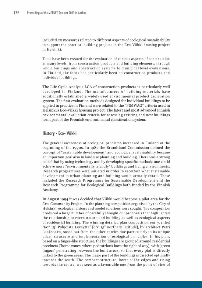
172 Proceedings of the METNET Seminar 2011 in Aarhus
included 20 measures related to different aspects of ecological sustainability to support the practical building projects in the Eco-Viikki housing project in Helsinki.
Tools have been created for the evaluation of various aspects of construction at many levels, from construction products and building elements, through whole buildings and construction systems to municipal level evaluations. In Finland, the focus has particularly been on construction products and individual buildings.
The Life Cycle Analysis LCA of construction products is particularly well developed in Finland. The manufacturers of building materials have additionally established a widely used environmental product declaration system. The first evaluation methods designed for individual buildings to be applied in practice in Finland were related to the “PIMWAG” criteria used in Helsinki’s Eco-Viikki housing project. The latest and most advanced Finnish environmental evaluation criteria for assessing existing and new buildings form part of the PromisE environmental classification system.
History - Eco- Viikki
The general awareness of ecological problems increased in Finland at the beginning of the 1990s. In 1987 the Brundtland Commission defined the concept of “sustainable development” and ecological sustainability became an important goal also in land use planning and building. There was a strong belief that by using technology and by developing specific methods one could achieve more “environmentally friendly” buildings and living environments. Research programmes were initiated in order to ascertain what sustainable development in urban planning and building would actually entail. These included the Research Programme for Sustainable Development and the Research Programme for Ecological Buildings both funded by the Finnish Academy.
In August 1994 it was decided that Viikki would become a pilot area for the Eco-Community Project. In the planning competition organised by the City of Helsinki, ecological visions and model solutions were sought. The competition produced a large number of carefully thought out proposals that highlighted the relationship between nature and building as well as ecological aspects of residential building. The winning detailed plan competition entry, titled “60° 15” Pohjoista Leveyttä” [60° 15” northern latitude], by architect Petri Laaksonen, stood out from the other entries due particularly to its unique urban structure and implementation of ecological principles. In his plan, based on a finger-like structure, the buildings are grouped around residential precincts (‘home zones’ where pedestrians have the right of way), with ‘green fingers’ penetrating between the built areas, so that every plot is directly linked to the green areas. The major part of the buildings is directed optimally towards the south. The compact structure, lower at the edges and rising towards the centre, was seen as a favourable one from the point of view of
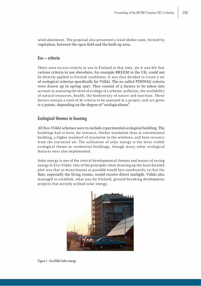
173Proceedings of the METNET Seminar 2011 in Aarhus
wind abatement. The proposal also presented a wind shelter zone, formed by vegetation, between the open field and the built-up area.
Eco – criteria
There were no eco-criteria in use in Finland at that time, yet it was felt that various criteria in use elsewhere, for example BREEM in the UK, could not be directly applied to Finnish conditions. It was thus decided to create a set of ecological criterias specifically for Viikki. The so-called PIMWAG criteria were drawn up in spring 1997. They consist of 5 factors to be taken into account in assessing the level of ecology of a scheme: pollution, the availability of natural resources, health, the biodiversity of nature and nutrition. These factors contain a total of 16 criteria to be assessed in a project, and are given 0-2 points, depending on the degree of “ecologicalness”.
Ecological themes in housing
All Eco-Viikki schemes were to include experimental ecological building. The buildings had to have, for instance, thicker insulation than in conventional building, a higher standard of insulation in the windows, and heat recovery from the extracted air. The utilisation of solar energy is the most visible ecological theme in residential buildings, though many other ecological features were also implemented.
Solar energy is one of the central developmental themes and means of saving energy in Eco-Viikki. One of the principles when drawing up the local detailed plan was that as many houses as possible would face southwards, so that the flats, especially the living rooms, would receive direct sunlight. Viikki also managed to establish, what was for Finland, ground-breaking development projects that actively utilised solar energy.
abatement. The proposal also presented a wind shelter zone, formed by vegetation, between the open field and the built-up area. Eco – criteria There were no eco-criteria in use in Finland at that time, yet it was felt that various criteria in use elsewhere, for example BREEM in the UK, could not be directly applied to Finnish conditions. It was thus decided to create a set of ecological criterias specifically for Viikki. The so-called PIMWAG criteria were drawn up in spring 1997. They consist of 5 factors to be taken into account in assessing the level of ecology of a scheme: pollution, the availability of natural resources, health, the biodiversity of nature and nutrition. These factors contain a total of 16 criteria to be assessed in a project, and are given 0-2 points, depending on the degree of “ecologicalness”. Ecological themes in housing All Eco-Viikki schemes were to include experimental ecological building. The buildings had to have, for instance, thicker insulation than in conventional building, a higher standard of insulation in the windows, and heat recovery from the extracted air. The utilisation of solar energy is the most visible ecological theme in residential buildings, though many other ecological features were also implemented. Solar energy is one of the central developmental themes and means of saving energy in Eco-Viikki. One of the principles when drawing up the local detailed plan was that as many houses as possible would face southwards, so that the flats, especially the living rooms, would receive direct sunlight. Viikki also managed to establish, what was for Finland, ground-breaking development projects that actively utilised solar energy.
Figure 1 - Eco.Viikki Solar energy
Other features adopted in Eco-Viikki projects were; district solar heating in eight separate neighbourhood blocks, adaptable wooden multi-storey houses, glazed balconies and conservatories, Viikki Development Projects Common themes in the housing production in Eco-Viikki include: separate metering of water consumption for each dwelling, conservatories/glazed balconies, water-saving
Figure 1 - Eco.Viikki Solar energy

174 Proceedings of the METNET Seminar 2011 in Aarhus
Other features adopted in Eco-Viikki projects were; district solar heating in eight separate neighbourhood blocks, adaptable wooden multi-storey houses, glazed balconies and conservatories,
Viikki Development Projects
Common themes in the housing production in Eco-Viikki include: separate metering of water consumption for each dwelling, conservatories/glazed balconies, water-saving plumbing fittings (e.g. toilets), and making use of rainwater in the communal yards. In another project, each individual dwelling had its own supply-extraction ventilation system together with heat recovery. The dwellings utilised passive solar energy through two-storey-high conservatories. One of the dwellings has its own solar-energy system.
An experimental 120-metre-long street section was built. Lime and cement and other reinforcement materials were mixed in with clay that had been dug up from the fields of Viikki. The stabilised clay was thus packed down on the lower part of the bearing layer of the street, replacing gravel and crushed aggregate
Eco–Viikki project’s results
The central ideas of the winning competition proposal, namely “the paved residential precincts into which the buildings feed” are the best features of the area. The eco-area has been built in a rather traditional way. The building types are mainly conventional ones: normal blocks of flats and terraced houses. The large number of glazed balconies and conservatories facing southwards is the most evident feature differing from convention. The different kinds of ecological “supplementary features”, such as the solar collectors, ventilation cowls on the roofs of the residential blocks, earth cellars, etc., also help to create an ecological image for the area.
The projects aimed to consume less heat, to save water, to keep noise under control and to avoid problems related to moisture problems. The most difficult environmental criteria to estimate in Viikki are the energy inherent to each building material
The Finnish sustainable methods /VTT Materiaalit ja Rakentaminen/
Viikki is a reflection of its time: in the mid-1990s ecology was almost a synonym for sustainable development. Only in recent years have also other elements of sustainable development emerged in the research and development.
National methods for environmental management of buildings and building products have been developed during recent years. These include the method
175Proceedings of the METNET Seminar 2011 in Aarhus
for the environmental assessment and environmental declarations of building products, EKA method and the classification method for buildings, PromisE.
EKA method
EKA is a Finnish national, voluntary method for environmental assessment of building products. The method describes the principles that should be followed in the environmental assessment of building products and introduces the format of environmental declarations. The procedure for environmental assessment and declaration of building products includes the following issues:
• principles for data collection and data handling (Life Cycle Inventory, LCI);
• generic environmental profiles for energy and transportation;
• the declaration format
• procedure of environmental assessment; auditing, approval and publication of declarations
• principles that one should follow when using the environmental profiles of building products within building design.
Tools for environmental assessment of building products
Different kinds of tools for the environmental assessment of buildings and products have been developed. These tools aid manufacturers to consider environmental aspects in product development and in environmental reporting. Tools has been developed for various materials and products, for example for cements, concrete products, natural stone products, underground structures, masonry products, wood products, flooring materials, building services systems and HVAC products and steel products. For example, with from the BERTTA tool, which has been developed for concrete manufactures, the effect of different kinds of parameters on the environmental profiles of concrete products and structures can be assessed.
Life cycle assessment LCA of buildings and building products
A database of environmental profiles of materials and products has been formulated on the basis of the results of inventory analyses.

176 Proceedings of the METNET Seminar 2011 in Aarhus
The program includes:
• Environmental profiles, costs and maintenance costs of building materials rinciples for data collection and data handling (Life Cycle Inventory, LCI);
• The structures for designing outdoor walls, indoor walls, roofs, floors, etc.
• Material quantity calculations
• Environmental profile calculation for designed structure
Result appears as a plot of environmental profile (emissions), energy- and raw-material use, and cost impact for the structure and whole building.
Service life assessment - ENNUS-TOOLS
ENNUS-programs have been developed for the service life assessment of building structures for designers. The programs help designers to determine parameters that affect the service life of the structure under scrutiny. These parameters include materials, details, workmanship, outdoor and indoor conditions, use conditions, and care and maintenance. ENNUS tools have been developed for concrete walls and balconies, steel facades and roofing and for wood outdoor walls /VTT Materiaalit ja Rakentaminen/.
Tools for environmental assessment of building products Different kinds of tools for the environmental assessment of buildings and products have been developed. These tools aid manufacturers to consider environmental aspects in product development and in environmental reporting. Tools has been developed for various materials and products, for example for cements, concrete products, natural stone products, underground structures, masonry products, wood products, flooring materials, building services systems and HVAC products and steel products. For example, with from the BERTTA tool, which has been developed for concrete manufactures, the effect of different kinds of parameters on the environmental profiles of concrete products and structures can be assessed. Life cycle assessment LCA of buildings and building products A database of environmental profiles of materials and products has been formulated on the basis of the results of inventory analyses. The program includes:
Environmental profiles, costs and maintenance costs of building materials rinciples for data collection and data handling (Life Cycle Inventory, LCI);
The structures for designing outdoor walls, indoor walls, roofs, floors, etc. Material quantity calculations Environmental profile calculation for designed structure
Result appears as a plot of environmental profile (emissions), energy- and raw-material use, and cost impact for the structure and whole building.
Service life assessment - ENNUS-TOOLS
ENNUS-programs have been developed for the service life assessment of building structures for designers. The programs help designers to determine parameters that affect the service life of the structure under scrutiny. These parameters include materials, details, workmanship, outdoor and indoor conditions, use conditions, and care and maintenance. ENNUS tools have been developed for concrete walls and balconies, steel facades and roofing and for wood outdoor walls /VTT Materiaalit ja Rakentaminen/.
Figure 2 - ENNUS Steel Programme Figure 2 - ENNUS Steel Programme
International sustainable criteria
When it comes to energy consumption, buildings account for a significant share of the total. Construction solutions that are based on recyclable and re-

177Proceedings of the METNET Seminar 2011 in Aarhus
usable materials, such as steel, help to reduce energy consumption and carbon emissions during the life cycle of buildings.
Environmental certification systems, LEED (Leadership in Energy & Environmental Design) and BREEAM (BRE Environmental Assessment Method), have been created to support building of environmentally responsible and resource-efficient buildings.
The Green Building rating system considers the whole life-cycle of buildings from their conception to operation and finally to their demolition. The purpose of Green Building rating system is to reduce the impacts of buildings to the environment through efficient resource use (energy, water, materials), protecting our health and reducing pollution, waste and other harmful effects.
Steel in construction has many benefits which link to Green Building – the structures are light, construction time short and material extremely recyclable. Looking at the certification systems steel gives opportunities to achieve points when materials are being considered, when looking at constructions and their lifecycle and when the disturbances of construction operation are assessed. Steel is directly connected to material issues and indirectly affects successful solutions in several issues.
LEED credits /www.ruukki.com/
LEED (Leadership in Energy & Environmental Design) is an internationally recognized green building certification system developed by the U.S. Green Building Council (USGBC), providing third-party verification that a building or community was designed and built using strategies aimed at improving performance across all the metrics that matter most: energy savings, water efficiency, CO2 emissions reduction, improved indoor environmental quality, and stewardship of resources and sensitivity to their impacts.
International sustainable criteria When it comes to energy consumption, buildings account for a significant share of the total. Construction solutions that are based on recyclable and re-usable materials, such as steel, help to reduce energy consumption and carbon emissions during the life cycle of buildings.
Environmental certification systems, LEED (Leadership in Energy & Environmental Design) and BREEAM (BRE Environmental Assessment Method), have been created to support building of environmentally responsible and resource-efficient buildings.
The Green Building rating system considers the whole life-cycle of buildings from their conception to operation and finally to their demolition. The purpose of Green Building rating system is to reduce the impacts of buildings to the environment through efficient resource use (energy, water, materials), protecting our health and reducing pollution, waste and other harmful effects.
Steel in construction has many benefits which link to Green Building – the structures are light, construction time short and material extremely recyclable. Looking at the certification systems steel gives opportunities to achieve points when materials are being considered, when looking at constructions and their lifecycle and when the disturbances of construction operation are assessed. Steel is directly connected to material issues and indirectly affects successful solutions in several issues. LEED credits /www.ruukki.com/ LEED (Leadership in Energy & Environmental Design) is an internationally recognized green building certification system developed by the U.S. Green Building Council (USGBC), providing third-party verification that a building or community was designed and built using strategies aimed at improving performance across all the metrics that matter most: energy savings, water efficiency, CO2 emissions reduction, improved indoor environmental quality, and stewardship of resources and sensitivity to their impacts.
Figure 3 - U.S.Green Building Council
Figure 3 - U.S.Green Building Council

178 Proceedings of the METNET Seminar 2011 in Aarhus
LEED scoring criteria includes following factors: site planning, sustainable site credit, innovation in design, energy and atmosphere credit, material and resources credit, and indoor environmental quality credit.
BREEAM credits /http://www.breeam.org/
BREEAM (BRE Environmental Assessment Method) is the world’s most widely used environmental assessment method for buildings. BREEAM assesses buildings against the seven separate criteria and provides an overall score: Pass, Good, Very good, Excellent or Outstanding. BREEM scoring criteria include, energy management, health and wellbeing, materials, waste and pollution.
LEED scoring criteria includes following factors: site planning, sustainable site credit, innovation in design, energy and atmosphere credit, material and resources credit, and indoor environmental quality credit. BREEAM credits /http://www.breeam.org/ BREEAM (BRE Environmental Assessment Method) is the world's most widely used environmental assessment method for buildings. BREEAM assesses buildings against the seven separate criteria and provides an overall score: Pass, Good, Very good, Excellent or Outstanding. BREEM scoring criteria include, energy management, health and wellbeing, materials, waste and pollution.
Figure 4 - BREEAM
BREEAM case: Vrangelsro, Sweden Vrangelso was the first Vrangelsro Industrial Building was the first BREEAM Europe 2008 Industrial assessment certified project. The development, ‘Vrangelsro 5.3,' is located in the southern city of Halmstad, on the west coast, and achieved a ‘Pass' rating at the post-construction assessment stage. It is the second project in Sweden to achieve BREEAM certification. The assessment scored well in Energy, Health & Wellbeing and Pollution.
Figure 5 - Vrangelsro Industrial Building
Figure 4 - BREEAM
BREEAM case: Vrangelsro, Sweden
Vrangelso was the first Vrangelsro Industrial Building was the first BREEAM Europe 2008 Industrial assessment certified project. The development, ‘Vrangelsro 5.3,’ is located in the southern city of Halmstad, on the west coast, and achieved a ‘Pass’ rating at the post-construction assessment stage. It is the second project in Sweden to achieve BREEAM certification. The assessment scored well in Energy, Health & Wellbeing and Pollution.
LEED scoring criteria includes following factors: site planning, sustainable site credit, innovation in design, energy and atmosphere credit, material and resources credit, and indoor environmental quality credit. BREEAM credits /http://www.breeam.org/ BREEAM (BRE Environmental Assessment Method) is the world's most widely used environmental assessment method for buildings. BREEAM assesses buildings against the seven separate criteria and provides an overall score: Pass, Good, Very good, Excellent or Outstanding. BREEM scoring criteria include, energy management, health and wellbeing, materials, waste and pollution.
Figure 4 - BREEAM
BREEAM case: Vrangelsro, Sweden Vrangelso was the first Vrangelsro Industrial Building was the first BREEAM Europe 2008 Industrial assessment certified project. The development, ‘Vrangelsro 5.3,' is located in the southern city of Halmstad, on the west coast, and achieved a ‘Pass' rating at the post-construction assessment stage. It is the second project in Sweden to achieve BREEAM certification. The assessment scored well in Energy, Health & Wellbeing and Pollution.
Figure 5 - Vrangelsro Industrial Building
Figure 5 - Vrangelsro Industrial Building

179Proceedings of the METNET Seminar 2011 in Aarhus
Green Strategy
Environmental- and energy-related issues were emphasized throughout the whole construction phases. All measures and proposals were checked during the design and construction stages to ensure they were at the forefront regarding environmental and energy issues. For example, as the building has too much waste heat, the aim is for future developments in the area to use this excess.
Materials such as the steel-frame, windows, floor and walls were checked by an environmental engineer before being installed in the building.
The building also has energy-efficient lightning: there are different levels of lightning in every room depending on what the room is being used for at any particular time.
The provision of lockers, showers, changing rooms and drying spaces has also been made, to encourage employees to cycle, walk or run to work.
Sustainable products and projects
Sandwhich panels /www.ruukki.com/
Green Strategy Environmental- and energy-related issues were emphasized throughout the whole construction phases. All measures and proposals were checked during the design and construction stages to ensure they were at the forefront regarding environmental and energy issues. For example, as the building has too much waste heat, the aim is for future developments in the area to use this excess. Materials such as the steel-frame, windows, floor and walls were checked by an environmental engineer before being installed in the building. The building also has energy-efficient lightning: there are different levels of lightning in every room depending on what the room is being used for at any particular time. The provision of lockers, showers, changing rooms and drying spaces has also been made, to encourage employees to cycle, walk or run to work. Sustainable products and projects Sandwhich panels /www.ruukki.com/
Figure 6 - Sandwhich panel
Sandwich panels are used in facades, roofs, compartmenting structures, partition walls and ceilings. The new energy panel solution creates savings in heating costs, leading in turn to significantly reduced carbon dioxide emissions generated by the use of the building. Ruukki’s sandwich panel walls have a high degree of thermal insulation and air-tightness by default. By using sandwich panel solutions, the LEED and BREEAM credit count can be increased for the building as well as lower heating energy costs and CO2 emissions.
Figure 6 - Sandwhich panel
Sandwich panels are used in facades, roofs, compartmenting structures, partition walls and ceilings. The new energy panel solution creates savings in heating costs, leading in turn to significantly reduced carbon dioxide emissions generated by the use of the building.
Ruukki’s sandwich panel walls have a high degree of thermal insulation and air-tightness by default. By using sandwich panel solutions, the LEED and BREEAM credit count can be increased for the building as well as lower heating energy costs and CO2 emissions.

180 Proceedings of the METNET Seminar 2011 in Aarhus
Fully integrated solar panel /www.ruukki.com/
Ruukki has developed a photovoltaic system that has been fully integrated into a façade to convert sun rays into energy. The solar power system does not depend on the sun’s warmth, only its radiation. The electricity generated is used either to meet the building’s own needs or is fed into the electricity grid.
Fully integrated solar panel /www.ruukki.com/ Ruukki has developed a photovoltaic system that has been fully integrated into a façade to convert sun rays into energy. The solar power system does not depend on the sun's warmth, only its radiation. The electricity generated is used either to meet the building's own needs or is fed into the electricity grid.
Figure 7 - Solar Power System
Additional storey construction Construction Companies have been devoping the technique to build extra stories above the old multi-story houses. By selling the new flats the rest of the house’s renovation can in many cases be financed. The extension is usually made with bearing steel structures outside the old frame. At the same time the building’s sustainability rating can usually be raised.
Figure 8 - Extra Storeys with Steel Structures
Figure 7 - Solar Power System
Additional storey construction
Construction Companies have been devoping the technique to build extra stories above the old multi-story houses. By selling the new flats the rest of the house’s renovation can in many cases be financed. The extension is usually made with bearing steel structures outside the old frame. At the same time the building’s sustainability rating can usually be raised.
Fully integrated solar panel /www.ruukki.com/ Ruukki has developed a photovoltaic system that has been fully integrated into a façade to convert sun rays into energy. The solar power system does not depend on the sun's warmth, only its radiation. The electricity generated is used either to meet the building's own needs or is fed into the electricity grid.
Figure 7 - Solar Power System
Additional storey construction Construction Companies have been devoping the technique to build extra stories above the old multi-story houses. By selling the new flats the rest of the house’s renovation can in many cases be financed. The extension is usually made with bearing steel structures outside the old frame. At the same time the building’s sustainability rating can usually be raised.
Figure 8 - Extra Storeys with Steel Structures
Figure 8 - Extra Storeys with Steel Structures

181Proceedings of the METNET Seminar 2011 in Aarhus
Conclusion
The growing demands for sustainability means that architects and engineers have to approach their projects differently than before and find new solutions. This gives great opportunities to the technically advanced metal products.
Tools have been created for the evaluation of various aspects of construction at many levels, from construction products and building elements, through whole buildings and construction systems to municipal level evaluations. In Finland there has been development for the sustainable assesment national tools and criteria lsuch as EKA, BERTTA, EcoProP and ENNUS. In addition, international methods like LEED and BREEAM are used to check the sustainability values. The environmental evaluation is to a great part still voluntary, but it will probably become a compulsory part of design and construction in the near future. By mastering the sustainable evaluation, the steel industry can even better than before issue the great properties of their products.

METNETA European network of institutions engaged in research and development in metal structures.
AimsThe general aim of the METnET network is to exchange information on current know-how in the field of metal structures among European research and development organizations. The network encourage the development of new products, facilitates better utilisation of services and business of companies involved with metal structures, supports innovation processes in companies involved in the manufacture and design of metal structures and promotes best practice and knowledge transfer between companies and research organizations in Europe.
MembersThe member organisations include universities and research establishments in Finland, Sweden, Denmark, Germany, czech republic, Hungary, Poland, russia, Ukraine, UK, Belarus, Portugal, Turkey, Greece. The current chairman of METnET is Dr Sc Lauri Tenhunen.
PublicationsFor the first time, at its Annual Seminar, which was held at Aarhus University in Denmark 2011, a scientific section has been included. The Scientific Papers and Technical reports presented over the two days are included in this publication which is available both in book form (iSBn 978-951-784-556-4) and as an e-book (iSBn 978-951-784-555-5). This publication is the first in the series to come. The papers have been refereed by a peer group.
Contact Publication ordersDir. Lauri Tenhunen, HAMK University of Applied Sciences HAMK publicationsVisamäentie 35 B, Fi-13100 Hämeenlinna, FinLAnD [email protected]. + 358 3 646 6410, Mobile + 358 40 560 2249lauri. tenhunen(at)hamk.fi
ELEcTrOnic
iSBn 978-951-784-555-5 (PDF)
iSSn 1795-424X
HAMKin e-julkaisuja 12/2011
PrinTED
iSBn 978-951-784-556-4
iSSn 1795-4231
HAMKin julkaisuja 8/2011
ROCKET