Aalto University

School of Engineering

Degree Programme in Mechanical Engineering

Matti Palin

Analysis of aerodynamic stability of theMetNet Entry and Descent vehicle withFINFLO simulations

Master’s ThesisEspoo, October 31, 2015

Supervisor: Professor Jukka Tuhkuri, Aalto UniversityAdvisors: Professor Timo Siikonen

Ari-Matti Harri, D.Sc. (Tech.) (Finnish MeteorologicalInstitute)

Aalto UniversitySchool of EngineeringDegree Programme in Mechanical Engineering

ABSTRACT OFMASTER’S THESIS

Author: Matti Palin

Title:Analysis of aerodynamic stability of the MetNet Entry and Descent vehicle withFINFLO simulations

Date: October 31, 2015 Pages: xiv + 86

Major: Aeronautical Engineering Code: K3004

Supervisor: Professor Jukka Tuhkuri

Advisors: Professor Timo SiikonenAri-Matti Harri, D.Sc. (Tech.) (Finnish MeteorologicalInstitute)

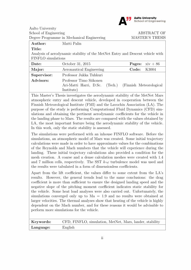
This Master’s Thesis investigates the aerodynamic stability of the MetNet Marsatmospheric entry and descent vehicle, developed in cooperation between theFinnish Meteorological Institute (FMI) and the Lavochin Association (LA). Thepurpose of the study is performing Computational Fluid Dynamics (CFD) sim-ulations and obtaining the pertinent aerodynamic coefficients for the vehicle inthe landing phase to Mars. The results are compared with the values obtained byLA, the most important feature being the aerodynamic stability of the vehicle.In this work, only the static stability is assessed.

The simulations were performed with an inhouse FINFLO software. Before thesimulations, an atmospheric model of Mars was created. Some initial trajectorycalculations were made in order to have approximate values for the combinationsof the Reynolds and Mach numbers that the vehicle will experience during thelanding. These initial trajectory calculations also provided a condition for themesh creation. A coarse and a dense calculation meshes were created with 1.4and 7 million cells, respectively. The SST k-ω turbulence model was used andthe results were tabulated in a form of dimensionless coefficients.

Apart from the lift coefficient, the values differ to some extent from the LA’sresults. However, the general trends lead to the same conclusions: the dragcoefficient is more than sufficient to ensure the designed landing speed and thenegative slope of the pitching moment coefficient indicates static stability forthe vehicle. Some heat load analyses were also carried out. Unfortunately, thesimulations converged only up to Ma = 1.9 and no results were obtained atlarger velocities. The thermal analyses show that heating of the vehicle is highlydependent on the Mach number, and for these reasons it would be advisable toperform more simulations for the vehicle.

Keywords: CFD, FINFLO, simulation, MetNet, Mars, lander, stability

Language: English

ii

Aalto-yliopistoInsinooritieteiden korkeakouluKonetekniikan koulutusohjelma

DIPLOMITYONTIIVISTELMA

Tekija: Matti Palin

Tyon nimi:MetNet-laskeutujan aerodynaamisen vakavuuden analysointi FINFLO-simulaatioilla

Paivays: 31. lokakuuta 2015 Sivumaara: xiv + 86

Paaaine: Lentotekniikka Koodi: K3004

Valvoja: Professori Jukka Tuhkuri

Ohjaajat: Professori Timo SiikonenTekniikan tohtori Ari-Matti Harri (Ilmatieteen Laitos)

Tassa diplomityossa tutkitaan Ilmatieteen Laitoksen ja Lavochin Associationin(LA) kehittaman Mars MetNet-laskeutujan aerodynaamista vakavuutta kayttaenlaskennallista virtausmekaniikkaa. Tavoitteena on ratkaista relevantit aerodynaa-miset kertoimet laskeutumisvaiheen aikana Marsiin. Tuloksia verrataan LA:n saa-miin arvoihin ja tarkeimpana tutkittavana ominaisuutena on aerodynaaminen va-kavuus. Tyossa tutkitaan vain staattista aerodynaamista stabiiliutta.

Laskentaan kaytettiin FINFLO-ohjelmaa. Marsin kaasukehasta luotiin malli en-nen simulaatioita. Lisaksi tehtiin ratalaskelmia laskeutujan laskeutumisvaiheenaikana kokemien Reynoldsin luvun ja Machin luvun arvojen saamiseksi. Ratalas-kelmat tuottivat myos ehdon, joka auttoi laskentaverkon luomisessa. Laskentaavarten luotiin harva ja tihea laskentaverkko, joissa oli 1,4 ja 7 miljoonaa lasken-takoppia. Turbulenssin kuvaukseen kaytettiin SST k-ω-mallia ja tulokset taulu-koitiin dimensiottomassa kerroinmuodossa.

Nostovoimakerrointa lukuun ottamatta tulokset erosivat jonkin verran LA:n saa-mista arvoista. Tuloksista voidaan kuitenkin tehda sama paatelma: laskeutu-jan vastuskerroin on enemman kuin riittava suunniteltuun laskeutumisnopeuteennahden ja pituusmomenttikertoimen negatiivinen kulmakerroin osoittaa laskeu-tujan olevan staattisesti stabiili. Laskenta ei kuitenkaan konvergoitunut suurem-milla Machin luvuilla kuin Ma = 1, 9 eika tuloksia saatu tata suuremmilla no-peuksilla. Lampotarkastelut osoittivat lisaksi laskeutujan pintalampotilan olevanvoimakkaasti riippuvainen Machin luvusta ja naista syista laskeutujalle suositel-laan suoritettavan lisaa simulaatioita.

Asiasanat: CFD, FINFLO, simulaatio, MetNet, Mars, laskeutuja, vaka-vuus

Kieli: Englanti

iii

iv

Acknowledgements

This thesis was created between January and September 2015 at the Me-chanical Engineering Department of the Aalto University in Otaniemi. Thisresearch was initiated and funded by the Finnish Meteorological Institute inorder to answer their need for aerodynamic research for the MetNet lander.

I wish to thank first and foremost professor Timo Siikonen for giving methe great occasion to work on this project. I am thankful for all the supportand guidance he has given me throughout the project. I am also gratefulto my supervisor Jukka Tuhkuri for the possibility to carry out my researchin the Department of Mechanical Engineering. Furthermore, I would like tothank Dr. Ari-Matti Harri and Harri Haukka for providing all the necessarymaterial for the work and for help along the way. Moreover, I wish to thankLucien Vienne (Universite de Toulon) for his conducive observations andcooperation during his internship in the department.

My gratitude goes also to the Department and staff of Mechanical Engi-neering of the Aalto University for providing me with the necessary facilities,know-how, and hardware for the demanding project.

Espoo, October 31, 2015

Matti Palin

v

vi

Abbreviations and Acronyms

CAD Computer-aided DesignDV Descent vehicleFMI Finnish Meteorological InstituteEDLS Entry, Descent and Landing SystemHEART High Energy Atmospheric Reentry TestLA Lavochkin AssociationCFD Computational Fluid DynamicsRITD Re-entry: inflatable technology development in Rus-

sian collaborationNASA National Aeronautics and Space AdministrationMIBD Main Inflatable Braking DeviceAIBD Additional Inflatable Braking DeviceMCD Mars Climate Database

vii

viii

List of symbols

Symbol description

a1 constant in the turbulence modelA (reference) areac speed of soundc reference lengthcf friction coefficientcp heat capacity at constant pressureCA axial force coefficientCD drag coefficientCm pitching moment coefficientCmα pitching moment coefficient slope with respect to the angle

of attackCmq pitching moment coefficient slope with respect to the pitch

rateCN normal force coefficientCNα normal force coefficient slope with respect to the angle of

attackCn Courant numberCL lift coefficientCLα lift coefficient slope with respect to the angle of attackD diameterE total internal energyFi flux in the ith cell

F flux through a cell faceF1, F2 blending functionsFA axial forceFN normal forceg acceleration of gravitygm ≈ 3.71 m

s, acceleration of gravity on the surface of Mars

ix

h enthalpyh altitude~i, ~j, ~k direction (unit) vectorsIz mass moment of inertiak kinetic energy of turbulenceKn Knudsen numberLD

lift-to-drag ratioLs solar longitude, the angle between Mars and the SunM momentMa Mach numberN number of valuesnj surface unit normal on a computational cellp pressureP production of kinetic energyq pitch rateq∞ = 1

2ρU2, the dynamic pressure

Q arbitrary quantityQs, Qi source termR specific gas constantRe Reynolds number referred to the main diameterRex Reynolds number referred to the x-coordinateRm ≈ 3386 km, the average radius of Marssi,j mean strain-rate tensorS reference areaS norm of strain-rate tensorScell face areat timeT temperatureT∞ free stream temperatureui velocity component

U , ~U free stream velocity; vehicle velocity magnitudeUτ friction velocityVi volume of a computation cellW vehicle weightxi, x, y, z, coordinatesy+ dimensionless distance from the wallα angle of attackα time derivative of the angle of attackα second time derivative of the angle of attackβw ballistic coefficient, calculated using the vehicle weight

x

βm traditional ballistic coefficient, calculated using the vehiclemass

β,β1, β2, β∗ constants in the turbulence model∆ differenceδi,j Kronecker delta. δi,j = 1 if i = j, and 0 otherwise.∆s height of the first mesh cell∆t time stepε turbulent dissipationγ specific heat ratioγ trajectory angle in radiansγ1, γ2 coefficients in the turbulence modelλ1,2 roots of the characteristic equationµ dynamic viscosityµT turbulent eddy viscosityω specific rate of dissipation of the turbulence kinetic energyρ medium densityσk1, σk2, σω1, σω2 constants in the turbulence modelτw wall shear stressτ , τi,j viscous stress tensor

xi

xii

Contents

1 Introduction and background 1

2 The MetNet Entry and Descent System 5

2.1 Background and history . . . . . . . . . . . . . . . . . . . . . 5

2.2 Mars atmospheric entry and descent conditions . . . . . . . . 6

2.2.1 Dependence of time and space . . . . . . . . . . . . . . 7

2.2.2 Gas state equation . . . . . . . . . . . . . . . . . . . . 7

2.2.3 The speed of sound on Mars . . . . . . . . . . . . . . . 9

2.2.4 Atmospheric density . . . . . . . . . . . . . . . . . . . 14

2.2.5 Atmospheric viscosity and Sutherland coefficients . . . 15

2.3 The vehicle & landing phases . . . . . . . . . . . . . . . . . . 15

2.3.1 MetNet DV in the transport configuration . . . . . . . 16

2.3.2 MetNet DV with inflated Main Inflatable Braking De-vice (MIBD) . . . . . . . . . . . . . . . . . . . . . . . . 17

2.3.3 MetNet DV after the inflation of Additional InflatableBraking Device (AIBD) . . . . . . . . . . . . . . . . . 18

2.4 Potential problems . . . . . . . . . . . . . . . . . . . . . . . . 18

2.5 Previous work . . . . . . . . . . . . . . . . . . . . . . . . . . . 20

2.5.1 Wind tunnel tests and their results . . . . . . . . . . . 21

2.5.2 Heat transfer tests . . . . . . . . . . . . . . . . . . . . 25

2.5.3 Drop tests . . . . . . . . . . . . . . . . . . . . . . . . . 26

3 Theoretical background 27

3.1 Aerodynamics of the vehicle . . . . . . . . . . . . . . . . . . . 27

3.2 Aerodynamic stability of the vehicle . . . . . . . . . . . . . . . 31

3.3 Stability criterion for the vehicle . . . . . . . . . . . . . . . . . 32

4 Calculation of landing trajectory 35

4.1 Parameter value ranges . . . . . . . . . . . . . . . . . . . . . . 37

4.2 Minimum entry angle for the atmospheric entry . . . . . . . . 42

xiii

5 FINFLO Solver 435.1 Solution algorithm . . . . . . . . . . . . . . . . . . . . . . . . 435.2 Turbulence model . . . . . . . . . . . . . . . . . . . . . . . . . 46

6 Simulations 496.1 Simulation setup . . . . . . . . . . . . . . . . . . . . . . . . . 49

6.1.1 Mesh Resolution . . . . . . . . . . . . . . . . . . . . . 496.1.2 Mesh generation and boundary conditions . . . . . . . 506.1.3 The input file . . . . . . . . . . . . . . . . . . . . . . . 53

6.2 Simulations and results . . . . . . . . . . . . . . . . . . . . . . 556.2.1 MetNet DV with inflated MIBD . . . . . . . . . . . . . 556.2.2 Penetrating part after the separation of the front shield

(AIBD case) . . . . . . . . . . . . . . . . . . . . . . . . 566.3 Observations on grid quality . . . . . . . . . . . . . . . . . . . 586.4 Surface temperatures . . . . . . . . . . . . . . . . . . . . . . . 59

6.4.1 The effect of Angle of Attack . . . . . . . . . . . . . . 606.4.2 The effect of free stream temperature . . . . . . . . . . 616.4.3 The effect of the Reynolds number . . . . . . . . . . . 616.4.4 The effect the Mach number . . . . . . . . . . . . . . . 626.4.5 Heat loads on AIBD . . . . . . . . . . . . . . . . . . . 63

7 Conclusions and discussion 65

A Input File Example 73

B Aerydynamic coefficients of the MIBD case 75

C Aerodynamic coefficients of the AIBD case 83

xiv

1

Chapter 1

Introduction and background

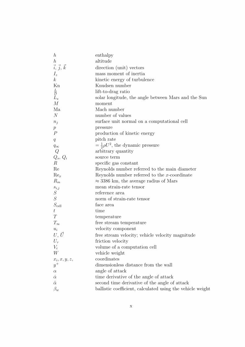
Within the framework of Mars exploration, the MetNet landing vehicle is arelatively new concept aimed to simplify and decrease the overall mass ofthe Entry, Descent and Landing Systems (EDLS). The current Mars roverconcepts, for example, are using an aeroshell, a parachute, airbags and adedicated lander structure or retro rockets [1, 2]. The MetNet concept,developed in collaboration by the Finnish Meteorological Institute (FMI),Instituto Nacional de Tecnica Aeroespacial (INTA), and the Russian SpaceResearch Institute, consists of deploying a pair of inflatable entry and descentsystems, eliminating the need for a parachute or thrusters and a rigid heatshield [3]. This way, the ratio of payload mass to overall mass could be in-creased and hence the mission payload efficiency is improved. See Figure 1.1for the landing scheme of the vehicle.

Shorthand for “Meteorological Network”, the MetNet project (a largeridea than only the lander) aspires to set up a network of science stationsaround the surface of Mars. These stations, equipped with a multitude ofinstruments, would survey the Martian atmosphere, meteorology, planetaryinterior, crust, and also magnetic environment performing simultaneous ob-servations at various locations on the Martian surface. This network wouldgreatly enhance our view of the atmospheric conditions on Mars on a largescale, compared with the local results acquired by the previous landers androvers. As the first step the mission plans to include deploying one precursorlander to Mars in 2022–2024 in order to demonstrate the technical robustnessand scientific potential of the MetNet Mission concept.

The MetNet vehicle design started in the year 2001 and an EDLS bodyprototype was built between 2001 and 2004. Wind tunnel and heat fluxtests have been conducted for the key components of the structure, but theproblem with these tests is that it is difficult to replicate the actual descentand landing conditions on Mars. This is because the composition of the

2

Figure 1.1: The descent phase of the MetNet lander [4].

atmosphere in Mars differs greatly from that on Earth. Even though thespeed of sound in these conditions is of the same order of magnitude as onEarth, the Mach number will still be large (exceeding Ma = 20). Thus it isout of the question to make one-to-one tests of the mission. [3, 5]

Since no similar landers have been sent to Mars before, a lot of researchhas to be done in order to verify its feasibility and to predict whether thechosen concept will succeed in the mission. There have been simulationsand tests of the structure, but a dedicated analysis and discussion aboutthe aerodynamic stability of the descent vehicle is still missing. This thesiscovers that topic. In 2014, FMI expressed the need for such work to the FluidMechanics Group of the Mechanical Engineering Department at the AaltoUniversity and the project started in January 2015. In September 2015, theproject was on display in European Planetary Science Congress 2015 [6].

Since analytical analyses of the complex geometry of the descent vehi-cle are close to impossible, numerical CFD-simulations are carried out. Theanalysis software of choice in this case is FINFLO. FINFLO is a general flowsolver based on the numerical solution of the differential equations describingviscous flow (the so-called Navier-Stokes equations). Originally developed for

3

the solution of compressible flows, FINFLO should be fit for the task thanksto its efficiency, turbulence modeling capabilities and its ability to solve com-plicated three-dimensional flow cases. It has already been used successfullyin many tasks in the fields of aerodynamics and applied thermodynamics [7].

The goal of the simulations is to acquire the aerodynamic features of thevehicle in the applicable configurations (the varying parameters will be theangle of attack, the Reynolds number and the Mach number) and heat fluxdata during the descent and landing phases. From the former it is possibleto draw conclusions of the aerodynamic stability of the vehicle. Should it beaerodynamically unstable, the EDLS design would have to be considerablymodified before sending the landing craft to Mars. Thus careful analysis ofthese features is in a decisive role in the development of the MetNet landingvehicle.

In this thesis, the aforementioned simulations are performed and conclu-sions are drawn from the analysis results. Trajectory calculations are alsoperformed in order to support the CFD simulations and to predict the perti-nent quantities related to the descent phase of the vehicle. Combined, theseresults form the aerodynamic analysis of the vehicle to the extent that isnecessary in its design.

This thesis was made in the facilities of the Fluid Mechanics Group inOtaniemi during the year 2015. It serves as the final thesis for the degree ofMaster of Science.

4

5

Chapter 2

The MetNet Entry and DescentSystem

2.1 Background and history

The idea for the lander was first conceived in the 1980’s by the FMI, theRussian Space Research Institute, Lavochkin Association (LA) and InstitutoNacional de Tecnica Aeroespacial. However, it was only in 2000 that thedevelopment work started. During the evolution of the project, five differentdescent system scenarios were analysed and a prototype was manufacturedin 2002. Martian environmental qualification testing was performed for theentry, descent and landing components of the selected variant. [3, 8, 9].

MetNet has generated several spin-off projects, including the NASA pro-jects called the High Energy Atmospheric Reentry Test and the HypersonicInflatable Aerodynamic Decelerator, and MetNet Entry, Descent and Land-ing System (EDLS) for Earth Reentry (RITD), as well as a MetNet precursormission (MMPM). The RITD concept, for example, consists of the same lan-der structure as in the MetNet Mars lander project (the main focus of thiswork) but with the intention of using it on Earth re-entry. This would bene-fit the existing projects already on Earth’s orbit by facilitating the logisticsbetween an orbiter and our planet. The MMPM project aims to send oneor two MetNet descent vehicles to Mars, serving as a technology and sciencedemonstration mission.

The most recent advancements of the MetNet project have been the im-provement of Mars’ atmospheric model [10], a mathematical modelling of thelander [11], the aforementioned wind tunnel tests [12, 13], feasibility analy-ses [14] and analysis of dynamic stability of the lander in the transonic flowregime [15]. The latter is clearly useful also in this thesis, even though the

6

analyses were done with an atmospheric model of the Earth and with a rel-atively low Mach number (the maximum Mach number in that documentwas Ma ≈ 2). The observations in the documents suggest that, in order toincrease its dynamic stability, the vehicle be given angular speed around itsaxis of symmetry during the entry phase:

(...) to provide MetNet DV stability in upper atmospheric layersthe angular rate of spinning after Main Inflatable Braking Device(MIBD) inflation should make 60 deg/s [15].

Additionally, it was concluded that the simulations resulted in static stabilityon certain conditions:

MetNet DV with inflated MIBD is statically stable at Knudsen num-bers < 0.3 and at continuous flow within the whole range of Machnumbers [15].

It was also noted that in the subsonic regime the vehicle would portray dy-namic instabilities in some cases, resulting in more constraints and require-ments for the entry and landing phases.

2.2 Mars atmospheric entry and descent con-

ditions

Analysing and understanding the atmospheric conditions on Mars is essentialin this project, since they directly influence the aerodynamic characteristicsof the lander. The speed of sound, for example, dictates the behaviour ofshock waves in the flow. In this section, the pertinent quantities are obtainedby deducing values from existing data and documentation.

In order to acquire the parameters related to the atmospheric conditionswhere the vehicle is designed to operate, alongside with other documentation,an on-line service called The Mars Climate Database is used [16]. Theirdocumentation gives a good representation of the service:

The Mars Climate Database (MCD) is a database of atmo-spheric statistics compiled from state-of-the art Global ClimateModel (GCM) simulations of the Martian atmosphere.

The GCM computes in 3D the atmospheric circulation takinginto account radiative transfer through the gaseous atmospheresas well as through dust and ice aerosols, includes a representationof the CO2 ice condensation and sublimation on the ground andin the atmosphere.

7

The model used to compile the statistics has been extensivelyvalidated using available observational data and aims at repre-senting the current best knowledge of the state of the Martianatmosphere given the observations and the physical laws whichgovern the atmospheric circulation and surface conditions on theplanet [17].

The service thus gives plausible initial values for our simulations. Therelevant parameters are the medium density and viscosity, atmospheric tem-perature and the speed of sound in the medium. MCD can provide thefirst three of these; the speed of sound has to be derived from the availableinformation and a relation between the mentioned quantities.

2.2.1 Dependence of time and space

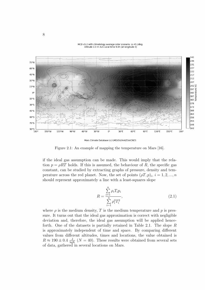
Before any calculations are made, it is important to take into considerationhow these quantities vary with space and time. Let us examine temperature,since it affects the value of many quantities. This can be carried out bycomparing temperature maps (see Figure 2.1) of the Martian surface.

As can be seen from Figure 2.1, the temperature is the lowest, as onecan expect, in the polar areas. Closer to the equator (latitude ≈ 0) the tem-perature is always higher by tens of Kelvins. Along the longitude, there isalso a warmer region (the positive longitudes in the figure). This area corre-sponds to the areas that are facing the Sun at a given time. In other words,it is daytime in those areas. Thus the longitudinal differences correspond today-vs-night differences.

Seasonal changes also have an effect on the temperature distribution. Thewarm region (the dark area in the figure) moves in latitude when the solarlongitude Ls changes. At summer solstice (Ls = 90◦) the warm region is inthe north and at winter solstice (Ls = 270◦) in the south. The movement ofthe warm region can be seen by setting the altitude to zero.

It can be seen (and shown by statistics) that the night-vs-day changes aresignificant. As a rule of thumb it can be said that the temperature on thesurface during the night is 50 K lower than during the day. The differencebetween “summer” and “winter” is approximately the same. It must be keptin mind that these results apply to the surface only.

2.2.2 Gas state equation

A crucial model that will be directly fed into FINFLO is an equation of statefor the gas. Therefore, it is essential to examine results from MCD and see

8

Figure 2.1: An example of mapping the temperature on Mars [16].

if the ideal gas assumption can be made. This would imply that the rela-tion p = ρRT holds. If this is assumed, the behaviour of R, the specific gasconstant, can be studied by extracting graphs of pressure, density and tem-perature across the red planet. Now, the set of points (ρT, p)i, i = 1, 2, ..., nshould represent approximately a line with a least-squares slope

R =

n∑i=1

ρiTipi

n∑i=1

ρ2iT

2i

, (2.1)

where ρ is the medium density, T is the medium temperature and p is pres-sure. It turns out that the ideal gas approximation is correct with negligibledeviation and, therefore, the ideal gas assumption will be applied hence-forth. One of the datasets is partially retained in Table 2.1. The slope Ris approximately independent of time and space. By comparing differentvalues from different altitudes, times and locations, the value obtained isR ≈ 190 ± 0.4 J

kgK(N = 40). These results were obtained from several sets

of data, gathered in several locations on Mars.

9

Table 2.1: Example data for calculating R. The solar longitude was set toLs = 225.0◦. Longitude 30.0E, Altitude 1000.0 m, ALS Local time 12.0 h (atall longitudes).

ρ[

kgm3

]T [K] p [Pa] ρT ρRT

0.0106 186.4330 370.7860 1.9786 376.09930.0108 183.0520 370.0510 1.9761 375.61830.0136 173.6950 444.2280 2.3637 449.2938

......

......

...0.0221 148.8300 627.9430 3.2927 625.88690.0213 147.9230 600.5140 3.1479 598.36930.0193 147.2660 543.4940 2.8488 541.5202

2.2.3 The speed of sound on Mars

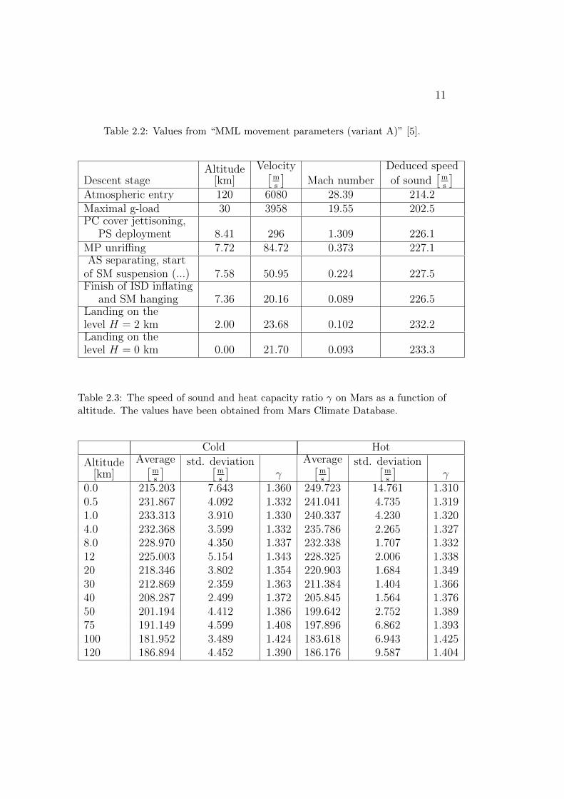
In Project Documentation for Selected concept by LA [5], some values canbe found for the velocity and Mach number of the case. The speed of soundcan thus be calculated from that data. Table 2.2 shows the data from thedocument and the results for the speed of sound. The deduced speed of soundwas obtained by dividing the velocity by the reported Mach number. TheMARS-GRAM 2001 atmospheric model was used to obtain these values.Validation of the model has indicated a “generally good” agreement withMCD for density [18] but no comments were made on the speed of sound.Some calculations by hand should therefore be made to verify these results.

According to Miettinen [19], the speed of sound can be calculated from

1

c2=

1

ρ

∂ρ

∂h

∣∣∣∣p

+∂ρ

∂p

∣∣∣∣h

, (2.2)

where c is the speed of sound and h is enthalpy. His work also gives therelations

∂ρ

∂h

∣∣∣∣p

=1

cp

∂ρ

∂T

∣∣∣∣p

(2.3)

∂ρ

∂p

∣∣∣∣h

=∂ρ

∂p

∣∣∣∣T

− 1

ρcp

∂ρ

∂T

∣∣∣∣p

(1 +

T

ρ

∂ρ

∂T

∣∣∣∣p

)(2.4)

10

Combining these gives

1

c2=

1

ρcp

∂ρ

∂T

∣∣∣∣p

+∂ρ

∂p

∣∣∣∣T

− 1

ρcp

∂ρ

∂T

∣∣∣∣p

(1 +

T

ρ

∂ρ

∂T

∣∣∣∣p

)=∂ρ

∂p

∣∣∣∣T

− T

ρ2cp

(∂ρ

∂T

∣∣∣∣p

)2

(2.5)As was noted before, the ideal gas assumption can be used. This implies

ρ =p

RT⇒

∂ρ∂p

∣∣∣∣T

= 1RT

∂ρ∂T

∣∣∣∣p

= − pRT 2

(2.6)

Now the equation for the speed of sound becomes simply

c =

√cp

cp −RRT (2.7)

This is merely a different formulation of c =√γRT , where γ is the specific

heat ratio, but more useful since the value of γ is not directly available.

The values of cp can be directly obtained from MCD and the scalar mapsreveal that it is strongly dependent of temperature. Since R is a constant,we can conclude that c is significantly dependent of T only.

For the purposes of this work, it would be very useful to tabulate valuesfor c. For this, we can use the conclusions made about the temperaturedistribution, ie. that it can be separated into “hot” and “cold” regions thatcorrespond to night-vs-day changes and seasonal changes.

The values for T and cp were obtained so that Ls = 0, local time 8 hours(at longitude 0). This way the hot values correspond approximately to pos-itive longitudes and the cold ones to negative longitudes. Two graphs wereobtained for each altitude: latitude ±10 degrees. The positive and negativelongitudes were separated and the two different latitudes were treated to-gether in order to increase the number of obtained values. Now the valuesfor c were calculated from Equation (2.7). The value of γ was also computedand averaged. The standard deviations for c were also computed.

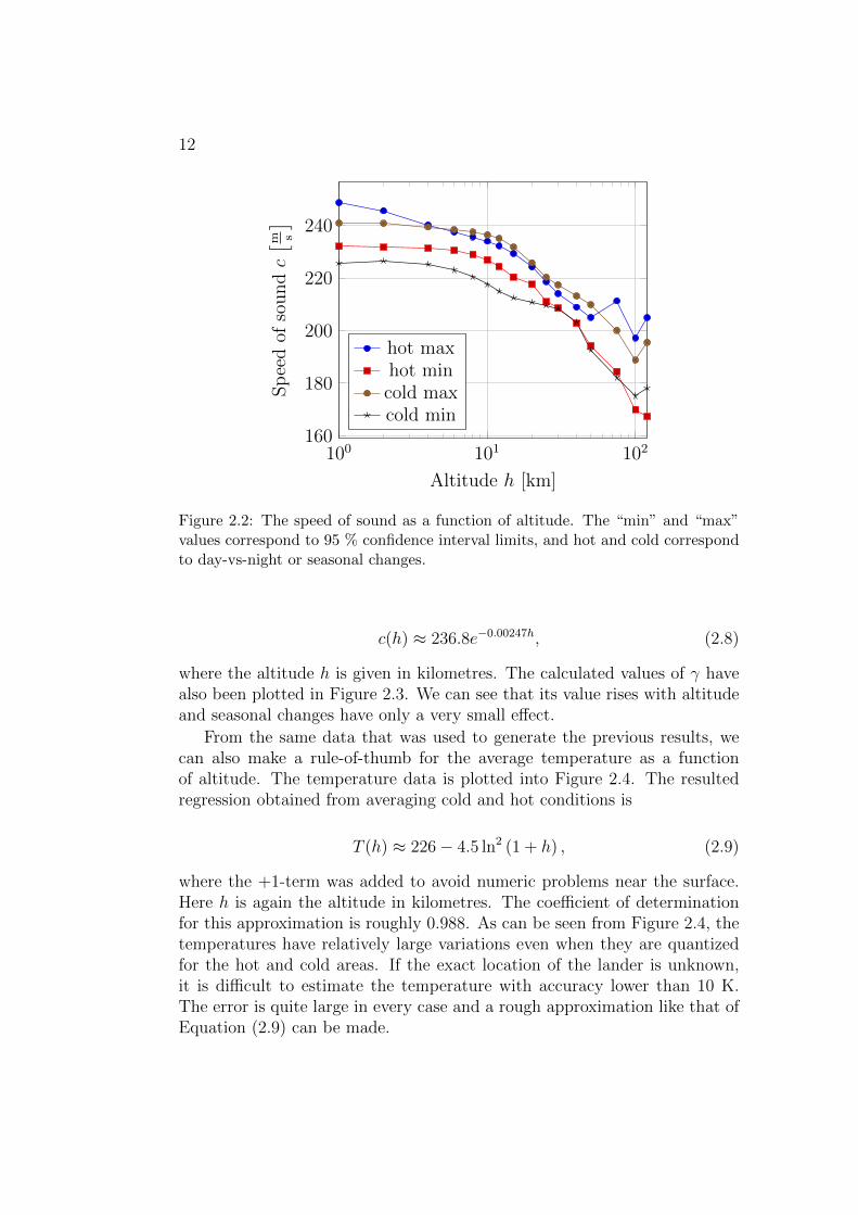
The results are presented in Table 2.3. Since there was some deviation inthe values for c, the 95 % confidence intervals have been calculated (N = 64).These have been drawn to Figure 2.2. As can be seen, the values from LAagree quite well with cold conditions and thus these values can be used fromnow on. Although the deviations in the value are significant, a rule-of-thumbwill be useful for later purposes. With regression, the following equation canbe made:

11

Table 2.2: Values from “MML movement parameters (variant A)” [5].

Descent stageAltitude

[km]

Velocity[ms

]Mach number

Deduced speed

of sound[

ms

]Atmospheric entry 120 6080 28.39 214.2Maximal g-load 30 3958 19.55 202.5PC cover jettisoning,

PS deployment 8.41 296 1.309 226.1MP unriffing 7.72 84.72 0.373 227.1AS separating, start

of SM suspension (...) 7.58 50.95 0.224 227.5Finish of ISD inflating

and SM hanging 7.36 20.16 0.089 226.5Landing on thelevel H = 2 km 2.00 23.68 0.102 232.2Landing on thelevel H = 0 km 0.00 21.70 0.093 233.3

Table 2.3: The speed of sound and heat capacity ratio γ on Mars as a function ofaltitude. The values have been obtained from Mars Climate Database.

Cold Hot

Altitude[km]

Average[ms

] std. deviation[ms

]γ

Average[ms

] std. deviation[ms

]γ

0.0 215.203 7.643 1.360 249.723 14.761 1.3100.5 231.867 4.092 1.332 241.041 4.735 1.3191.0 233.313 3.910 1.330 240.337 4.230 1.3204.0 232.368 3.599 1.332 235.786 2.265 1.3278.0 228.970 4.350 1.337 232.338 1.707 1.33212 225.003 5.154 1.343 228.325 2.006 1.33820 218.346 3.802 1.354 220.903 1.684 1.34930 212.869 2.359 1.363 211.384 1.404 1.36640 208.287 2.499 1.372 205.845 1.564 1.37650 201.194 4.412 1.386 199.642 2.752 1.38975 191.149 4.599 1.408 197.896 6.862 1.393100 181.952 3.489 1.424 183.618 6.943 1.425120 186.894 4.452 1.390 186.176 9.587 1.404

12

100 101 102160

180

200

220

240

Altitude h [km]

Sp

eed

ofso

un

dc[ m s

]hot maxhot mincold maxcold min

Figure 2.2: The speed of sound as a function of altitude. The “min” and “max”values correspond to 95 % confidence interval limits, and hot and cold correspondto day-vs-night or seasonal changes.

c(h) ≈ 236.8e−0.00247h, (2.8)

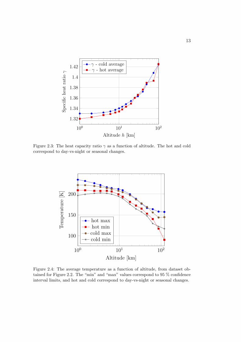
where the altitude h is given in kilometres. The calculated values of γ havealso been plotted in Figure 2.3. We can see that its value rises with altitudeand seasonal changes have only a very small effect.

From the same data that was used to generate the previous results, wecan also make a rule-of-thumb for the average temperature as a functionof altitude. The temperature data is plotted into Figure 2.4. The resultedregression obtained from averaging cold and hot conditions is

T (h) ≈ 226− 4.5 ln2 (1 + h) , (2.9)

where the +1-term was added to avoid numeric problems near the surface.Here h is again the altitude in kilometres. The coefficient of determinationfor this approximation is roughly 0.988. As can be seen from Figure 2.4, thetemperatures have relatively large variations even when they are quantizedfor the hot and cold areas. If the exact location of the lander is unknown,it is difficult to estimate the temperature with accuracy lower than 10 K.The error is quite large in every case and a rough approximation like that ofEquation (2.9) can be made.

13

100 101 102

1.32

1.34

1.36

1.38

1.4

1.42

Altitude h [km]

Sp

ecifi

chea

tra

tioγ

γ - cold averageγ - hot average

Figure 2.3: The heat capacity ratio γ as a function of altitude. The hot and coldcorrespond to day-vs-night or seasonal changes.

100 101 102

100

150

200

Altitude [km]

Tem

per

ature

[K]

hot maxhot mincold maxcold min

Figure 2.4: The average temperature as a function of altitude, from dataset ob-tained for Figure 2.2. The “min” and “max” values correspond to 95 % confidenceinterval limits, and hot and cold correspond to day-vs-night or seasonal changes.

14

Table 2.4: Gas density as a function of altitude, gathered from MCD [16].

Altitude [km] Density ρ× 103[

kgm3

]0.1 16.31230.5 15.51411.0 14.64762.0 13.20725.0 10.012211 5.847625 1.7512437 0.4265855 0.0551580 0.002187

100 0.000167120 0.0000109140 0.0000006

2.2.4 Atmospheric density

Even though the seasonal fluctuation of density is significant at certain timeperiods, quantifying these differences would not contribute to this work. Thisis because the seasonal changes are of the order of 10 %. The aerodynamicsof the vehicle are not very sensitive to the Reynolds number, so this kindof error does not impair the results of this work. Thus we only make anapproximation of the density as a function of altitude and around the latitudezero at a given season.

The results were collected by obtaining two sets of values from each alti-tude: latitudes ±30◦ and the global average was calculated for these. Timesetting was chosen to be Ls = 0◦, local time 9 hours. The results are inTable 2.4. A regression for the logarithm of density gives:

ρ(h) ≈{e−4.113−0.095h if h ≤ 46 kme−2.320−0.134h if h > 46 km

, (2.10)

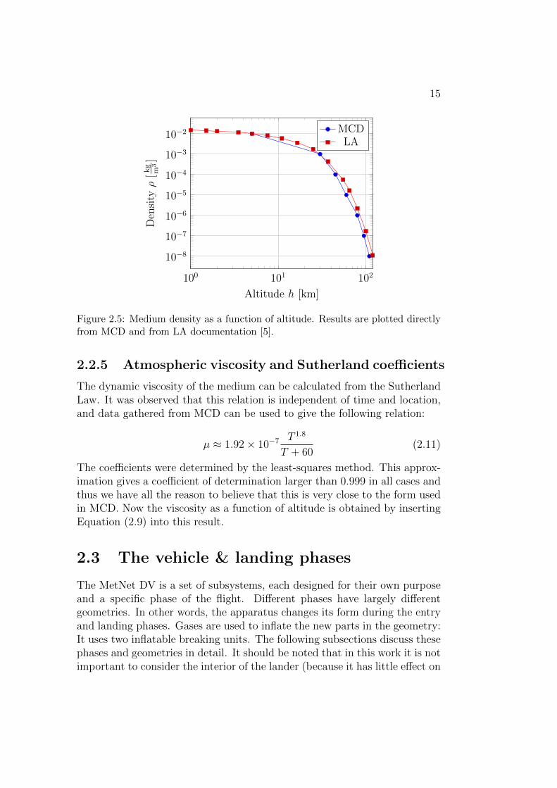
where h is in kilometres. This gives a coefficient of determination of 0.998and thus it can be used as a rule-of-thumb for the density in this work.The equation was cut into two pieces in order to increase accuracy at highaltitudes. Additionally, in Figure 2.5 is a graph of the results for the mediumdensity. The results from LA documentation were also drawn into the graphand they are in good agreement as expected.

15

100 101 102

10−8

10−7

10−6

10−5

10−4

10−3

10−2

Altitude h [km]

Den

sityρ

[kg

m3]

MCDLA

Figure 2.5: Medium density as a function of altitude. Results are plotted directlyfrom MCD and from LA documentation [5].

2.2.5 Atmospheric viscosity and Sutherland coefficients

The dynamic viscosity of the medium can be calculated from the SutherlandLaw. It was observed that this relation is independent of time and location,and data gathered from MCD can be used to give the following relation:

µ ≈ 1.92× 10−7 T 1.8

T + 60(2.11)

The coefficients were determined by the least-squares method. This approx-imation gives a coefficient of determination larger than 0.999 in all cases andthus we have all the reason to believe that this is very close to the form usedin MCD. Now the viscosity as a function of altitude is obtained by insertingEquation (2.9) into this result.

2.3 The vehicle & landing phases

The MetNet DV is a set of subsystems, each designed for their own purposeand a specific phase of the flight. Different phases have largely differentgeometries. In other words, the apparatus changes its form during the entryand landing phases. Gases are used to inflate the new parts in the geometry:It uses two inflatable breaking units. The following subsections discuss thesephases and geometries in detail. It should be noted that in this work it is notimportant to consider the interior of the lander (because it has little effect on

16

the aerodynamic characteristics of the vehicle; and because the interior partsare not modeled in the simulations) and thus only the outside geometry isconsidered.

2.3.1 MetNet DV in the transport configuration

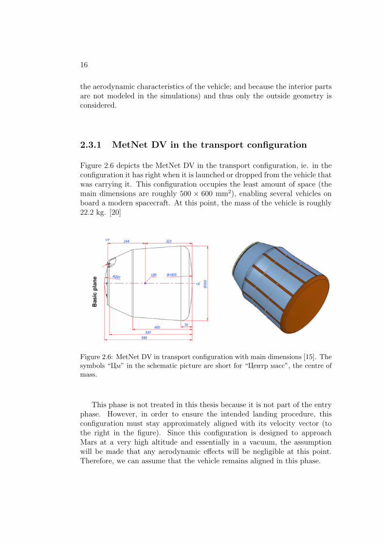
Figure 2.6 depicts the MetNet DV in the transport configuration, ie. in theconfiguration it has right when it is launched or dropped from the vehicle thatwas carrying it. This configuration occupies the least amount of space (themain dimensions are roughly 500 × 600 mm2), enabling several vehicles onboard a modern spacecraft. At this point, the mass of the vehicle is roughly22.2 kg. [20]

Figure 2.6: MetNet DV in transport configuration with main dimensions [15]. Thesymbols “Цм” in the schematic picture are short for “Центр масс”, the centre ofmass.

This phase is not treated in this thesis because it is not part of the entryphase. However, in order to ensure the intended landing procedure, thisconfiguration must stay approximately aligned with its velocity vector (tothe right in the figure). Since this configuration is designed to approachMars at a very high altitude and essentially in a vacuum, the assumptionwill be made that any aerodynamic effects will be negligible at this point.Therefore, we can assume that the vehicle remains aligned in this phase.

17

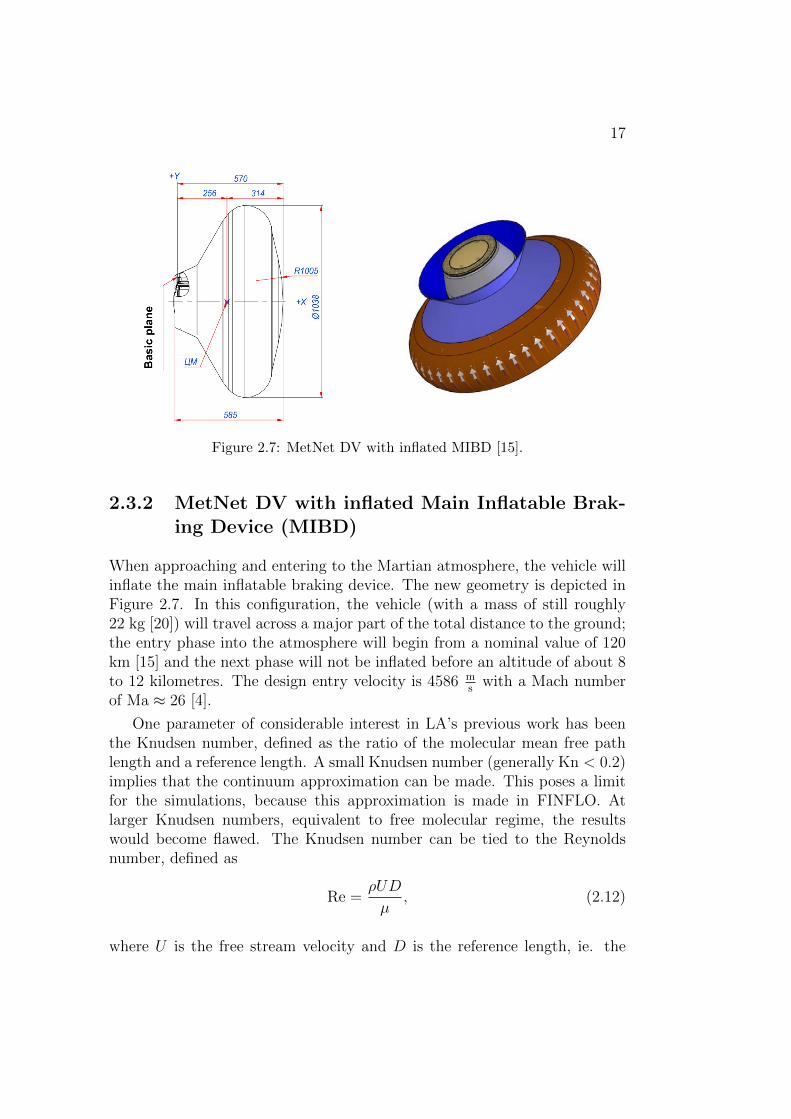
Figure 2.7: MetNet DV with inflated MIBD [15].

2.3.2 MetNet DV with inflated Main Inflatable Brak-ing Device (MIBD)

When approaching and entering to the Martian atmosphere, the vehicle willinflate the main inflatable braking device. The new geometry is depicted inFigure 2.7. In this configuration, the vehicle (with a mass of still roughly22 kg [20]) will travel across a major part of the total distance to the ground;the entry phase into the atmosphere will begin from a nominal value of 120km [15] and the next phase will not be inflated before an altitude of about 8to 12 kilometres. The design entry velocity is 4586 m

swith a Mach number

of Ma ≈ 26 [4].

One parameter of considerable interest in LA’s previous work has beenthe Knudsen number, defined as the ratio of the molecular mean free pathlength and a reference length. A small Knudsen number (generally Kn < 0.2)implies that the continuum approximation can be made. This poses a limitfor the simulations, because this approximation is made in FINFLO. Atlarger Knudsen numbers, equivalent to free molecular regime, the resultswould become flawed. The Knudsen number can be tied to the Reynoldsnumber, defined as

Re =ρUD

µ, (2.12)

where U is the free stream velocity and D is the reference length, ie. the

18

diameter of the vehicle. It can be shown that [21]

Kn =Ma

Re

√γπ

2(2.13)

Equation (2.13) can be used to make an approximation for the altitude lim-iting the region of the continuum approximation. Inserting the definitions ofthe Mach number and the Reynolds number, the equation becomes

Kn(h) =µ(h)

ρ(h)c(h)D

√γπ

2< 0.2 (2.14)

Now equations (2.8)-(2.11) can be used to solve the maximum altitude forthe continuum approximation numerically. As the diameter of the vehicle inthe higher altitudes is D = 1 m, the result is approximately h < 97.5 km.

2.3.3 MetNet DV after the inflation of Additional In-flatable Braking Device (AIBD)

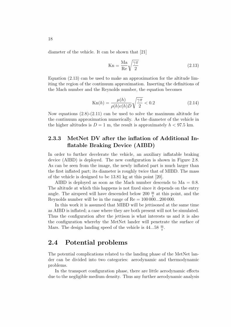
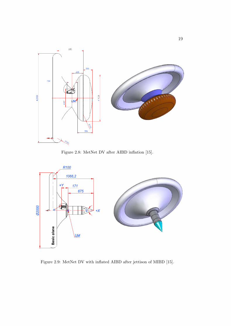
In order to further decelerate the vehicle, an auxiliary inflatable brakingdevice (AIBD) is deployed. The new configuration is shown in Figure 2.8.As can be seen from the image, the newly inflated part is much larger thanthe first inflated part; its diameter is roughly twice that of MIBD. The massof the vehicle is designed to be 13.81 kg at this point [20].

AIBD is deployed as soon as the Mach number descends to Ma = 0.8.The altitude at which this happens is not fixed since it depends on the entryangle. The airspeed will have descended below 200 m

sat this point, and the

Reynolds number will be in the range of Re = 100 000...200 000.In this work it is assumed that MIBD will be jettisoned at the same time

as AIBD is inflated; a case where they are both present will not be simulated.Thus the configuration after the jettison is what interests us and it is alsothe configuration whereby the MetNet lander will penetrate the surface ofMars. The design landing speed of the vehicle is 44...58 m

s.

2.4 Potential problems

The potential complications related to the landing phase of the MetNet lan-der can be divided into two categories: aerodynamic and thermodynamicproblems.

In the transport configuration phase, there are little aerodynamic effectsdue to the negligible medium density. Thus any further aerodynamic analysis

19

Figure 2.8: MetNet DV after AIBD inflation [15].

Figure 2.9: MetNet DV with inflated AIBD after jettison of MIBD [15].

20

of this phase can be ignored. However, the aerodynamics of the subsequentphases could impose requirements for the actual launch from the carryingvehicle. For example, as it has been noted, the vehicle should be giventhe angular speed, mentioned in Section 2.1, around its axis of symmetry.Also, the entry speed and angle are to be carefully chosen. Thermodynamicproblems related to the transport configuration phase can also be dismisseddue to the negligible medium density.

After the vehicle has entered the atmosphere, the aerodynamic effectscan cause issues for the descent stage. It is imperative that the vehicle landupright. In other words, it must not turn over during the flight. This iscalled aerodynamic stability and it is the most important point in this work;the simulations and analyses aim to verify this condition. This requirementis equally important for the two phases discussed earlier. It is possible toestimate whether or not such a reversal will happen by creating a model of themovement of the vehicle around itself. Once such a model has been created,a condition for its stability can be formulated. This is carried out startingfrom Section 3.1. Also, the final speed, pertaining to the drag coefficient ofthe vehicle, needs to be under a certain limit value in order for the vehicleto be able to function properly after landing.

Another problem with AIBD is its size. It will take more time to inflate,compared to MIBD, and this could potentially be a problem for the aerody-namic effects and stability. If, for example, the part remains in a partiallyinflated state for a non-negligible time and, for this reason, the vehicle be-comes asymmetric for some time, it is clear that the aerodynamic effects willalso be asymmetric. This could cause the vehicle to become dynamicallyunstable. This problem is not covered in this work.

The imaginable thermodynamic problem of the landing phase is the ex-cessive warming of the vehicle. LA has already produced some results forthe heat fluxes during the descent phase, but the simulations in this workprovide also some pertinent results.

2.5 Previous work

Documents from LA, FMI and Babakin Space Center provide documentationof analyses and tests done for the lander. In this section, the results aregathered and analysed in order to support and to provide reference values forthis work. This way, the results of the simulations done in the context of thiswork can be easily compared with the values obtained by LA. The pertinentresults are the wind tunnel tests (from which the important aerodynamiccoefficients can be obtained), heat tests and drop tests.

21

A large part of the documentation is from the first years of the currentcentury and the design has been altered a number of times. The numericalvalues of many parameters change between documents, the most noticeableones being the diameters and the masses of the different configurations. Inthe latest documentation, RITD Final Report from 2015, the diameter isfixed to exactly D = 1 m for the MIBD phase and D = 2 m for the AIBDphase. The mass (in the transport phase) is fixed to 22.2 kg. In this doc-ument, the entry velocity is fixed to 4586 m

sinstead of the older value of

6080 ms. [4]

2.5.1 Wind tunnel tests and their results

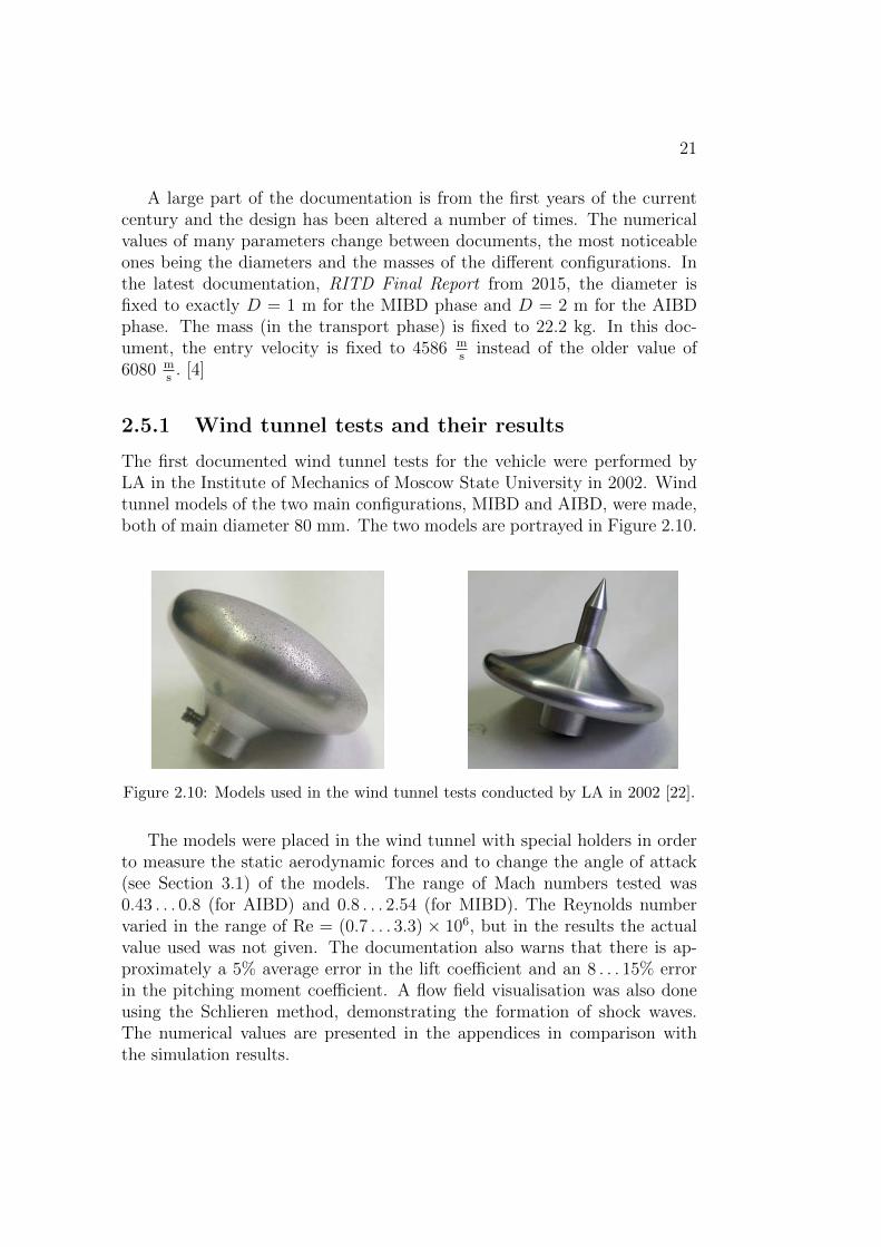
The first documented wind tunnel tests for the vehicle were performed byLA in the Institute of Mechanics of Moscow State University in 2002. Windtunnel models of the two main configurations, MIBD and AIBD, were made,both of main diameter 80 mm. The two models are portrayed in Figure 2.10.

Figure 2.10: Models used in the wind tunnel tests conducted by LA in 2002 [22].

The models were placed in the wind tunnel with special holders in orderto measure the static aerodynamic forces and to change the angle of attack(see Section 3.1) of the models. The range of Mach numbers tested was0.43 . . . 0.8 (for AIBD) and 0.8 . . . 2.54 (for MIBD). The Reynolds numbervaried in the range of Re = (0.7 . . . 3.3) × 106, but in the results the actualvalue used was not given. The documentation also warns that there is ap-proximately a 5% average error in the lift coefficient and an 8 . . . 15% errorin the pitching moment coefficient. A flow field visualisation was also doneusing the Schlieren method, demonstrating the formation of shock waves.The numerical values are presented in the appendices in comparison withthe simulation results.

22

More recent work conducted by LA in 2014 includes the wind tunnel testsof the MIBD configuration in order to determine its dynamic (transient) aero-dynamic features. The studied coefficient is the pitch-damping coefficient,denoted in the work by mωz

z and more commonly by Cmq . A model with adiameter of 74.2 mm was built using 3D printing technology. The model wasplaced in another wind tunnel but this time it was set up so that it can movefreely after being given an initial angle of attack. This way it is possible tostudy the dynamic behaviour of the vehicle as a function of Mach numberand the initial angle of attack. A high-speed camera was used to pick up themovements of the model.

In these tests, the free stream Mach number was 0.85 . . . 1.53 and theReynolds number was (1.25 . . . 3.0) × 105, respectively [13]. When the flowin the tunnel was turned on, the model started to oscillate at a frequencybetween 10 and 20 Hz. The high speed camera tracked these movements. Aninteresting feature is the static angle of attack or the maximum (absolute)value of the angle of attack that the model reaches during each vibrationcycle. For example, at Ma = 0.85 and at an initial angle of attack of 10◦, themodel started to oscillate, after approximately 0.2 seconds, between roughly−10◦ and 10◦. Here the static angle of attack would be 10◦.

Following the evolution of the static angle of attack, the results can besummarised as follows:

• At Ma < 1 pitch damping will occur at static angles of attack ofα < 10◦. The static angle of attack will tend to zero.

• At Ma > 1 the static angle of attack will gravitate to approximately10◦ and oscillate around that value.

Cases with an initial angle of attack larger than 10◦ were not examined inthese tests. The conclusion is that the dynamic wind tunnel tests do supportthe dynamic stability of the vehicle. In other words, the angle of attack staysrestrained and the vehicle is dynamically stable (Lyapunov stable).

Other documentation can also be found where values for the aerodynamiccoefficients are presented (for example in Feasibility of MetNet EDLS to Earthre-entry [20] and Analysis of and inflatable EDLS’ dynamic stability in thetransonic regime [15]), but the procedure by which these were obtained isnot well explained: the only comment made is that they are “calculationresults”. Therefore, these values will be treated as estimations. However,the interesting feature of these results is that they also treat the case offlight in rarified gas. For this reason it is reasonable to also comment onthese results.

23

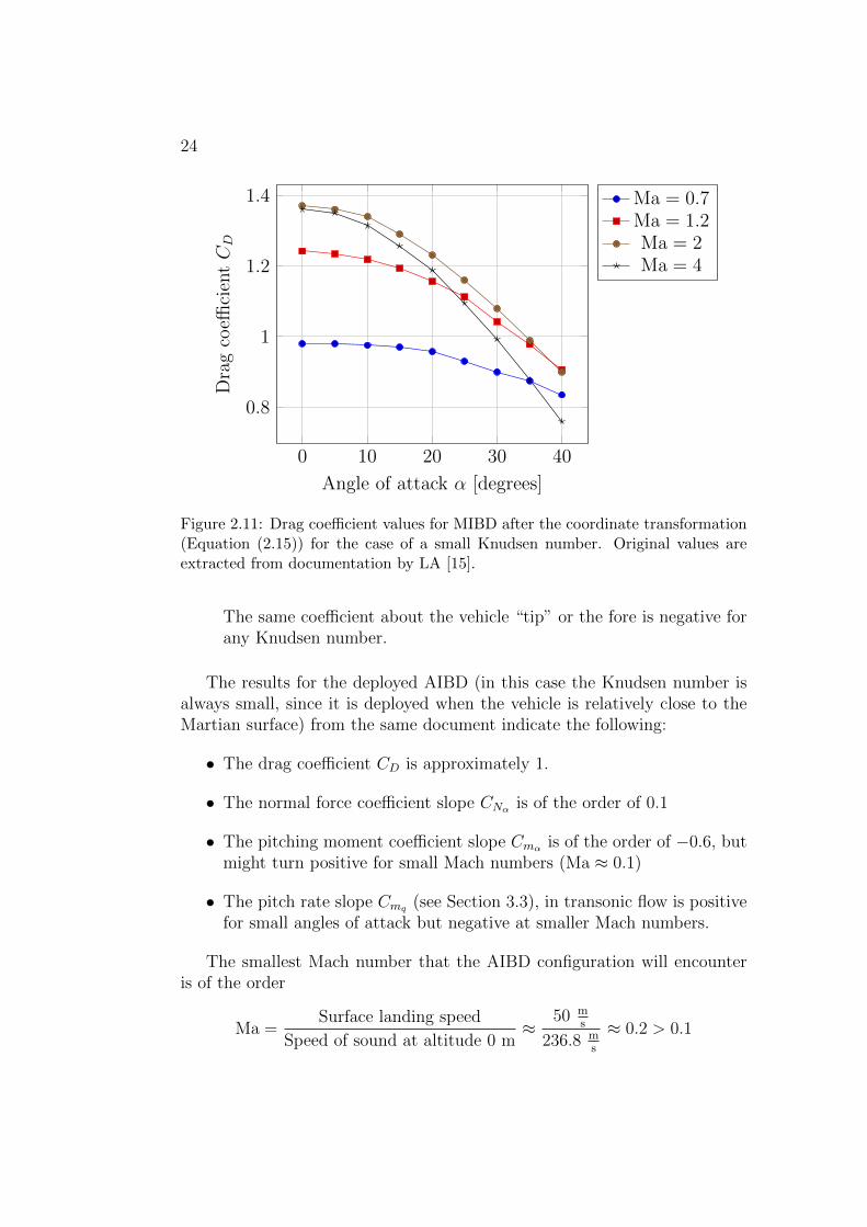
In order to use these static results in the context of this work, furthertreatment must be given to the numerical values. This is because the co-efficients given are the axial coefficient CA and the normal coefficient CNwhereas the coefficients we are interested in are the lift coefficient CL anddrag coefficient CD (see Section 3.1). The conversion between these is

CL = CN cosα− CA sinαCD = CN sinα + CA cosα

(2.15)

It is crucial to note that in LA’s convention, the angle of attack is definedas exactly the opposite to our definition. Therefore, when converting theseresults, a negative value must be used for α. An example result from thetransformation is in Figure 2.11.

Additionally, the pitching moment coefficient is calculated with respectto different points. LA’s calculation results were tabulated with respect tothe nose of the vehicle [15], whereas the FINFLO results are calculated withrespect to the centre of mass. The conversion between these can be calculatedfrom

Cmcom = Cmnose + CNxcom − xnose

D, (2.16)

where Cmcom and Cmnose are the pitching moment coefficients relative to thecentre of mass and nose, respectively, and xcom and xnose are the locations ofthe centre of mass and the nose, respectively, in the chosen coordinate system.For the case of MIBD (see Figure 2.7), we see that xcom − xnose ≈ 314 mm. Asfor AIBD (see Figure 2.9), the corresponding value is xcom − xnose ≈ 675 mm.

After the treatment for the values for MIBD [15], the following generaltrends can be seen:

• In the large Knudsen number regime (rarified gas) the drag coefficientCD is approximately between 1.5 and 2 for realistic angles of attack(α < 30◦) and diminishes with growing α. For lower Knudsen num-bers (continuous flow) the value is approximately 1.0 for small Machnumbers and raises to 1.4 for the larger Mach numbers.

• The absolute value of the lift coefficient CL grows in a linear fashionfor realistic angles of attack, as expected. The slope CLα = ∂CL

∂αis

approximately −0.8 1rad

for small Knudsen numbers and −0.1 1rad

forlarge Knudsen numbers.

• The pitching moment coefficient about the centre of mass is positivefor large Knudsen numbers and negative for small Knudsen numbers.

24

0 10 20 30 40

0.8

1

1.2

1.4

Angle of attack α [degrees]

Dra

gco

effici

entCD

Ma = 0.7Ma = 1.2Ma = 2Ma = 4

Figure 2.11: Drag coefficient values for MIBD after the coordinate transformation(Equation (2.15)) for the case of a small Knudsen number. Original values areextracted from documentation by LA [15].

The same coefficient about the vehicle “tip” or the fore is negative forany Knudsen number.

The results for the deployed AIBD (in this case the Knudsen number isalways small, since it is deployed when the vehicle is relatively close to theMartian surface) from the same document indicate the following:

• The drag coefficient CD is approximately 1.

• The normal force coefficient slope CNα is of the order of 0.1

• The pitching moment coefficient slope Cmα is of the order of −0.6, butmight turn positive for small Mach numbers (Ma ≈ 0.1)

• The pitch rate slope Cmq (see Section 3.3), in transonic flow is positivefor small angles of attack but negative at smaller Mach numbers.

The smallest Mach number that the AIBD configuration will encounteris of the order

Ma =Surface landing speed

Speed of sound at altitude 0 m≈

50 ms

236.8 ms

≈ 0.2 > 0.1

25

Therefore, it is likely that, according to the previous results, the pitchingmoment coefficient slope stays negative. This indicates static stability forthe AIBD configuration. In the dynamic regime, the fourth conclusion in theprevious results suggests that right after the AIBD deployment the staticangle of attack would not be 0 degrees but about five to ten degrees. Thusthe only phase of the flight where the lander would not be (Lyapunov) stable,according to these results, is in the high Knudsen number regimes or at veryhigh altitudes.

2.5.2 Heat transfer tests

Another concern of the MetNet project is the potential problems related tothe thermodynamic effects or, in practise, the heating of the vehicle. Thiscauses sublimation of the thermal protection coating applied to the vehicleand it could also damage the instruments in the payload. These effects havealso been analysed by LA.

A calculation of the warming and ablation was documented in ProjectDocumentation for Selected Concept in 2002. Fourier’s law and heat equationwas used in accordance with the Stefan–Boltzmann law for the boundaryconditions. With these, the heat fluxes and temperatures were calculated asa function of time at several points around the vehicle. When the propertiesof the thermal protection coating were known, the amount of linear ablation(material loss in millimeters) was also calculated. The atmospheric entryangle was selected to be 12◦ [5].

The results from this document indicate that the maximum temperaturereached during the descent stage is just under 700 ◦C right on the surfaceof the vehicle. The temperature of the internal structure would not surpass200 ◦C. Ablation of the protective coating was calculated to be approximately1.1 mm. This warm-up would occur at approximately 50 seconds into theatmospheric entry and last for about one minute. In the end, at landing, thetemperature throughout the structure would be around 200 ◦C.

In Small (mini) landing station systems tests from 2002 is a description ofthermal protection systems (the frontal area of the lander in MIBD configu-ration) tests and their results. Small sample plates of the used material weretested in a Hall accelerator. The heat fluxes used were based on calculationresults. For example, the maximum heat flux would occur at the stagnationpoint in the frontal area and the heat flow would reach, according to thedocumentation, approximately 450 kW

m2 . Eight different samples were thensubjected to various heat fluxes for a time period of 38 ± 0.5 seconds. Theresults show that the external layer reached 510 ◦C and the temperature ofthe internal layer did not exceed 220 ◦C [22].

26

2.5.3 Drop tests

In order to determine the forces and accelerations during the impact intothe Martian surface, drop tests were performed by LA. The design impactspeed is 60 m

sand the mass of the penetrating part is 5.02 kg. With this

initial data, calculations have again been performed for the vehicle as well asfull-scale model drop tests. In these tests, the inclination angle was variedbetween 0 and 30 degrees. The soil models used in the calculations weregranular (sandy), average density (clay) and rock.

The calculation results were documented as graphs of g-load and se-quences of images portraying the penetrating phase. They indicate that themaximum g-load is approximately 500, which appears when the horizontalspeed is 15 m

sand inclination is 30 degrees (granular soil). Travel depth into

the soil reached a maximum of 230 mm. [5]Full-scale drop tests were also described in the documentation. Two lan-

der modules were used for the tests: a dynamic model with properties closeto the actual vehicle; and an overall-mass model for the verification of testconditions and methodology. Two soil models were used here: sandy andfirm soil. [23]

The documentation does not provide any results from the drop tests.Therefore, the only conclusion that can be drawn from these documents isthat landing speed should not exceed 60 m

s.

27

Chapter 3

Theoretical background

In this chapter we take a theoretical look of the MetNet landing vehicle,define the pertinent terms and quantities and finally introduce requirementsfor it. Even though the geometry is far different from traditional airplanes,general aeronautical definitions can be applied to the vehicle. The applicablequantities are calculated in order to assess the qualities of the vehicle.

3.1 Aerodynamics of the vehicle

Like any object, the MetNet lander disturbs the medium around it whenflying through the Martian atmosphere. The molecules colliding into theobject change their direction, causing a momentum change in the flow. Forexample, if the vehicle is advancing slightly turned in relation to the incomingflow, some particles will pass it from over the vehicle and some under thevehicle. Due to the asymmetry of the geometries experienced by the particles,they will attain different speeds and pressures. In short, the process is similarto the effects that cause lift and drag force in airplane wings.

In order to describe and calculate the pertinent aerodynamic quantitiesfor the vehicle, a coordinate system will have to be defined. The origin islocated wherever it is defined when the calculation mesh is created. In thecases created in this work, the origin is set to the nose or tip of the vehicle.The x-axis needs to be consistent with FINFLO: the positive x-axis is the flowdirection (if the angle of attack is zero). Note that this is the inverse of whatwas implied in Figure 2.7. See Figure 3.1 for the coordinate definitions inFINFLO. The y- and z-axes form the right-handed coordinate system withthe x-axis. Note also that due to the rotational symmetry of the vehicle,the actual directions of the y- and z-axes remain vague. However, in themesh creation, the xy-plane is defined as the symmetry plane. The direction

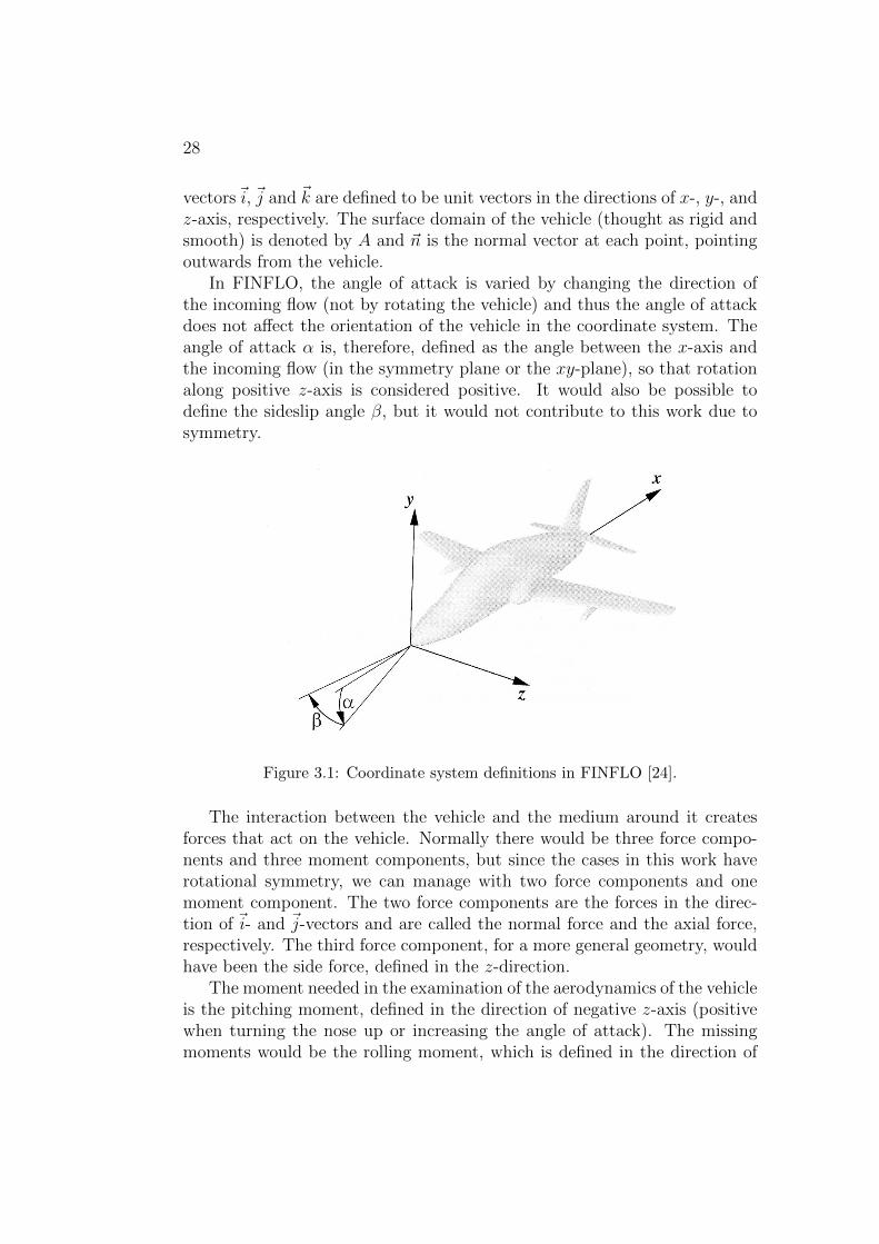
28

vectors~i, ~j and ~k are defined to be unit vectors in the directions of x-, y-, andz-axis, respectively. The surface domain of the vehicle (thought as rigid andsmooth) is denoted by A and ~n is the normal vector at each point, pointingoutwards from the vehicle.

In FINFLO, the angle of attack is varied by changing the direction ofthe incoming flow (not by rotating the vehicle) and thus the angle of attackdoes not affect the orientation of the vehicle in the coordinate system. Theangle of attack α is, therefore, defined as the angle between the x-axis andthe incoming flow (in the symmetry plane or the xy-plane), so that rotationalong positive z-axis is considered positive. It would also be possible todefine the sideslip angle β, but it would not contribute to this work due tosymmetry.

Figure 3.1: Coordinate system definitions in FINFLO [24].

The interaction between the vehicle and the medium around it createsforces that act on the vehicle. Normally there would be three force compo-nents and three moment components, but since the cases in this work haverotational symmetry, we can manage with two force components and onemoment component. The two force components are the forces in the direc-tion of ~i- and ~j-vectors and are called the normal force and the axial force,respectively. The third force component, for a more general geometry, wouldhave been the side force, defined in the z-direction.

The moment needed in the examination of the aerodynamics of the vehicleis the pitching moment, defined in the direction of negative z-axis (positivewhen turning the nose up or increasing the angle of attack). The missingmoments would be the rolling moment, which is defined in the direction of

29

negative x-axis, and the yawing moment, defined in the direction of negativey-axis. Again, the two latter moments disappear due to symmetry.

D.F. Kurtulus has formulated, using momentum balance, a general equa-tion for the calculation of the aerodynamic forces on an arbitrary shapeimmersed in a fluid [25]. For the stationary case, the axial and normal forcesbecome

~FA =

∫∫A

[−ρ(~U · ~n

)~U + p~n− τ · ~n

]·~i dS

~FN =

∫∫A

[−ρ(~U · ~n

)~U + p~n− τ · ~n

]·~j dS

(3.1)

where ~U is the local velocity vector and τ is the viscous stress tensor. Inpractise, the terms in Equation 3.1 are obtained from momentum fluxes.The components of the viscous tensor are

τi,j = τj,i = µ

[∂uj∂xi

+∂ui∂xj− ∂uk∂xk

δi,j

]−(ρu

′′i u

′′j − δi,j

2

3ρk

)(3.2)

In this notation, ui represent the three velocity components and xi representthe coordinates, k is turbulence kinetic energy, δi,j is the Kronecker delta,

and ρu′′i u

′′j is the Reynolds stress. These terms will be discussed in Chapter 5.

The pitching moment about an arbitrary point P of the vehicle is then

~MP =

∫∫A

([ρ(~U · ~n

)~U + p~n− τ · ~n

]× ~r)· ~k dS (3.3)

where ~r is the distance from the reference point to the integration point.Another way of presenting these quantities is the coefficient form

FN = CN12ρU2S

FA = CA12ρU2S

M =∣∣∣ ~M ∣∣∣ = Cm

12ρU2Sc

(3.4)

here CN , CA and Cm are the normal, the axial and the moment coefficientabout the centre of mass, respectively; ρ is the medium density, U is the freestream velocity, S is the reference area, and c is the reference length. In thecase of the MetNet lander, we can set the reference length to be the largestdiameter of a given geometry (c = 1 m for the MIBD case and c = 2 m forthe AIBD case) and the area to be the cross-sectional area at the point ofthe largest diameter, resulting in S = π

4c2.

30

The aerodynamic coefficients CA, CN and Cm are in the centre of attentionin this work. They can be thought of as the aerodynamic characteristics of thevehicle. With them, it is possible to make calculations about the behaviourof the vehicle when it is advancing in the medium. They depend stronglyon the angle of attack of the vehicle and the Mach and Reynolds numbers.However, a more common form for the force coefficients is the use of liftand drag coefficients CL and CD, coefficients for forces relative to the outsideenvironment and not the vehicle. They can be easily calculated from the axialand normal coefficients from Equation (2.15). These are the coefficients thatFINFLO is able to calculate, alongside the moment coefficient.

The pitching moment coefficient about the centre of mass Cm is also ofgreat importance in this work. Two derivative terms can be defined from it:

• Cmα = ∂Cm∂α

is the variation of the pitching moment coefficient withthe angle of attack or slope of pitching moment coefficient the withrespect to the angle of attack. Here it is assumed that pitching momentcoefficient varies approximately linearly with the angle of attack. Inreality, approximate values are calculated for this term so that Cmα ≈∆Cm∆α

. The derivative is approximated by difference terms. Thus thevalue for this coefficient can be approximately computed if the pitchingmoment coefficient is calculated for several angles of attack.

• The slope of pitching moment coefficient with respect to the pitch rateCmq = dCm

d( αc2U ), where q is the pitch rate or the angular rate of the vehicle

around the z-axis. Due to rotational symmetry, in this work it can beequated to the time derivative of the angle of attack, q = dα

dt= α. Note

that the so called normalization is carried out in the differentiation inorder to give sensible units for the derivative and to make it independentof free flow speed. Computing a value for this coefficient would requireforcing the angle of attack to oscillate at different frequencies and thencompute how much the pitching moment coefficient is affected by thatfrequency. This would require very extensive computations and is notcalculated in this work.

It should be noted that in this work the cross-section of the vehicle isapproximated as a perfect circle. In reality, the realised geometry will be,for the solid parts, as close to a circle as it is possible to fabricate, but theinflatable parts will actually form a 12-gon. Now a question arises: can the12-gon be approximated as a circle in the context of this work? The areaof a regular 12-gon is, omitting the proof, exactly 3 times the outer radiussquared. Thus the ratio of the areas, when we think of a circle and a 12-gonsuperimposed, is 3/π ≈ 0.9549. Since the aerodynamic forces are directly

31

proportional to the cross-sectional area, we can conclude that the error inthe aerodynamic coefficients between a 12-gon and a circle is less than 5 percent. This is an acceptable error and thus we can from now on approximatethe cross sections as circles.

3.2 Aerodynamic stability of the vehicle

As already discussed in Section 2.4, the vehicle must be designed so that itstays upright during the descent stage. In other words, the angle of attackmust remain constrained. This is equivalent to the aerodynamic stability ofthe vehicle and it can be divided into two parts: static and dynamic stability.A general definition for static stability is provided by Roskam [26]:

Static stability is defined as the tendency of an airplane to developforces or moments which directly oppose an instantaneous pertur-bation of a motion variable from a steady-state flight condition.

A definition for dynamic stability is also provided by Roskam:

Dynamic stability is defined as the tendency of the amplitudes ofthe perturbed motion of an airplane to decrease to zero or to valuescorresponding to a new steady state at some time after the cause ofthe disturbance has stopped.

In order to use the definition of static stability in the context of this work,we will interpret “steady-state flight condition” as a flight condition wherethe angle of attack is constant. A “perturbation” would then mean anychange in angle of attack from this constant value. If the vehicle is staticallystable, it would then, according to the first definition, develop forces andmoments that oppose this change. For example, if the steady-state value forthe angle of attack is zero and some perturbation occurs so that the angleof attack becomes positive, the aerodynamic effects would tend to decreasethis value back to zero and the pitching moment would be negative.

The definition of dynamic stability concerns the amplitude of the per-turbed motion variable and is fulfilled if the amplitude diminishes to zero.Simulations of these phenomena require time accurate simulations that wouldtake several orders of magnitude more calculation time (see the previous sub-section). In this work, such simulations are not run, but as computers becomefaster and faster it is imaginable that some day these simulations could bedone.

The orientation of the vehicle in relation to the incoming flow can com-pletely be defined with the angle of attack (α) alone and it is the only motion

32

variable in the model related to the orientation. This is due to the previ-ously discussed rotational symmetry. Other motion variables that could bediscussed would be the velocities of the vehicle along different coordinates (xand y), and one could discuss the stability for these variables as well. Otherkinds of stability would not be important in the design of the vehicle since, forexample, it is specifically desirable that the vehicle slows itself down as muchas possible. The evolution of velocity variables are treated in the trajectorycalculations in Chapter 4.

3.3 Stability criterion for the vehicle

In order to approach the stability of the vehicle from a mathematical pointof view, an equation of motion must be developed. As mentioned, the onlymotion variable of interest in the stability analysis is the angle of attack αand the aerodynamic stability of the vehicle is thus related to its evolutionswith time. Newton’s second law applied for rotational systems states thatthe net moment applied to a body is proportional to the angular accelerationit obtains: ∑

Mz = Izd2α

dt2(3.5)

Rotation is interpreted here as the change of angle of attack α. Thus themoments are calculated around the z-axis. The only moment applied to thebody is the aerodynamic moment around the z-axis. Next, we will make aTaylor-type approximation for the moment:

Mz ≈Mz(α = 0) +dMz

dαα +

dMz

d(αc2U

) αc2U

(3.6)

Here α = dαdt

= q is the pitch rate or the time derivative of the angle of attack.This quantity can be thought as analogous to angular velocity. Additionallywe can assume Mz(α = 0) = 0 considering the vehicle as symmetric. Thepitch rate term has already been discussed in Section 3.1. Now the coefficientforms from Equation (3.4) can be used:

Mz ≈dCmdα

α1

2ρU2Sc+

dCm

d(αc2U

) αc2U

1

2ρU2Sc = Cmαq∞Scα+Cmq

q∞Sc2

2Uα (3.7)

Here the dynamic pressure is 12ρU2 = q∞. With this result and Newton’s

second law, we obtain the differential equation of the angular movement forthe MetNet lander:

33

Izα−q∞Sc

2

2UCmq α− q∞ScCmαα = 0 (3.8)

Equation (3.8) is a homogenic second-order linear ordinary differentialequation corresponding to an equation of harmonic motion with damping.The solution of this equation involves the use of a characteristic equationand its roots. Omitting the calculation steps, the roots of the characteristicequation are

λ1,2 =1

2

q∞Sc2

2UIzCmq ±

√(−q∞Sc

2

2UIzCmq

)2

+ 4q∞Sc

IzCmα

(3.9)

It can be shown that the solutions for Equation (3.8) are stable (theamplitudes of the oscillations will tend to zero as time increases) if and onlyif the real parts of both of the roots are negative. For this next part only, letus make a shorthand notation − q∞Sc2

UIzCmq = a and − q∞Sc

IzCmα = b. Since all

the quantities are real numbers, this condition becomes

• If a2 − 4b ≥ 0 (⇔ λ1,2 ∈ R), the plus-signed condition yields a >√a2 − 4b ≥ 0 ⇒ a > 0 and a2 > a2 − 4b⇒ b > 0 or a, b > 0. The

condition for the minus-signed root is automatically fulfilled.

• or, if a2 − 4b < 0 ⇒ λ1,2 = 12

(−a± i

√4b− a2

)where i2 = −1 and

Re(λ1,2) = −a2< 0⇒ a > 0 and a ∈ R⇒ b > a2

4> 0.

Recognising that all the other quantities are positive, the stability condi-tion becomes a, b > 0 or Cmα < 0 and Cmq < 0. This is an intuitive result:a negative slope for the pitching moment coefficient means that the pitchingmoment obtains negative values when α is positive, thus creating a momentthat opposes the perturbation from zero angle of attack. A negative valuefor the slope of the pitching moment with the pitch rate means that an in-crease in the speed at which a (positive) angle of attack grows increases theopposing (negative) pitching moment, thus damping the oscillations. TheCmq term is, therefore, sometimes called the damping derivative.

34

35

Chapter 4

Calculation of landing trajectory

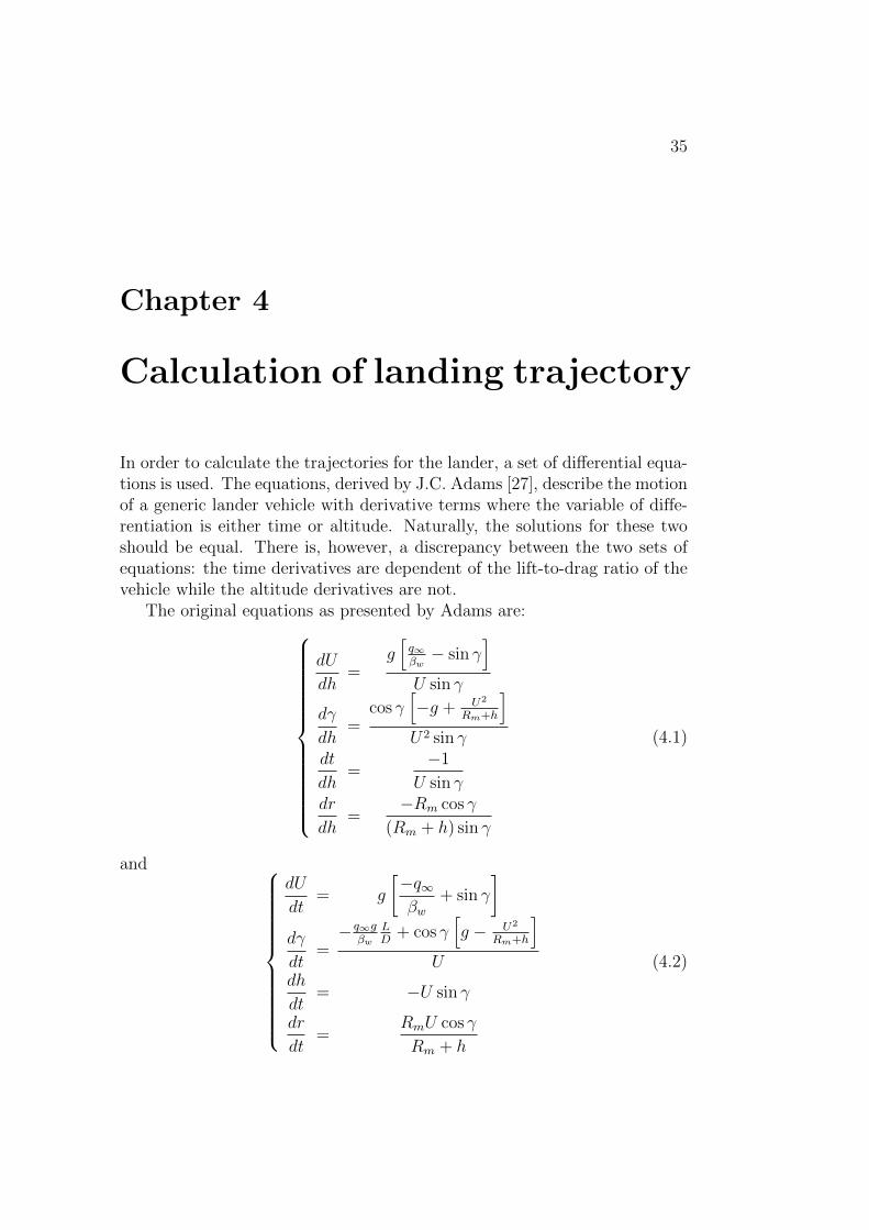
In order to calculate the trajectories for the lander, a set of differential equa-tions is used. The equations, derived by J.C. Adams [27], describe the motionof a generic lander vehicle with derivative terms where the variable of diffe-rentiation is either time or altitude. Naturally, the solutions for these twoshould be equal. There is, however, a discrepancy between the two sets ofequations: the time derivatives are dependent of the lift-to-drag ratio of thevehicle while the altitude derivatives are not.

The original equations as presented by Adams are:

dU

dh=

g[q∞βw− sin γ

]U sin γ

dγ

dh=

cos γ[−g + U2

Rm+h

]U2 sin γ

dt

dh=

−1

U sin γdr

dh=

−Rm cos γ

(Rm + h) sin γ

(4.1)

and

dU

dt= g

[−q∞βw

+ sin γ

]dγ

dt=− q∞g

βwLD

+ cos γ[g − U2

Rm+h

]U

dh

dt= −U sin γ

dr

dt=

RmU cos γ

Rm + h

(4.2)

36

where

• U is the vehicle velocity magnitude

• γ is the flight path angle in radians (positive below the horizontal ;π

2would be “straight down”)

• h is the altitude

• r is the flight range above the surface

• t is the flight time

• Rm is the radius of Mars ; Rm ≈ 3386 km

• g is the acceleration of gravity; it can be calculated from g(h) = gm

(Rm

Rm+h

)2

;

gm ≈ 3.71 ms2 is the acceleration of gravity on the surface of Mars.

• q∞ = 12ρU2 is dynamic pressure at a given altitude. The density ρ can

be calculated from Equation (2.10).

• βw is the ballistic coefficient βw = WCDA

; W = mg is the vehicle weight(in Newtons – notice this uncommon notation); CD is the drag coef-ficient and A is the reference area used in the determination of dragcoefficient. In our case A = π

4D2 where D is the diameter of the vehicle.

Although the ballistic coefficient is usually expressed as mass dividedby the drag coefficient times reference area, here the choice of using theweight of the vehicle instead ensures that the units of the equations areconsistent.

• LD

= CLCD

is the lift-to-drag ratio of the vehicle.

The aforementioned discrepancy can be easily corrected using differentialalgebra. Since the term affected by the lift-to-drag ratio is γ, we can write

dγ

dh=dγ

dt

dt

dh=− q∞g

βwLD

+ cos γ[g − U2

Rm+h]

U

−1

U sin γ=

q∞gβw

LD

+ cos γ[−g + U2

Rm+h]

U2 sin γ

This is the equation that will replace the term for dγdh

in Equation (4.1). Theother equations are consistent.

Another noteworthy feature that can be seen from the equation set isthat it is easy to solve the landing speed. It can be solved by setting dU

dt= 0

and solving U from that equation, resulting in

37

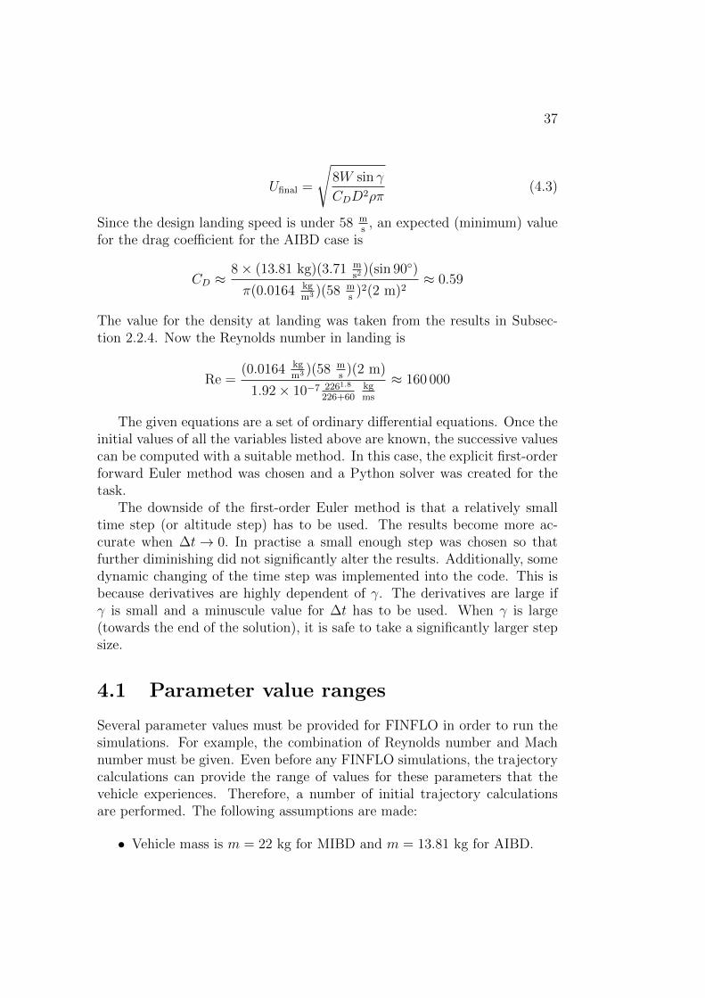
Ufinal =

√8W sin γ

CDD2ρπ(4.3)

Since the design landing speed is under 58 ms, an expected (minimum) value

for the drag coefficient for the AIBD case is

CD ≈8× (13.81 kg)(3.71 m

s2 )(sin 90◦)

π(0.0164 kgm3 )(58 m

s)2(2 m)2

≈ 0.59

The value for the density at landing was taken from the results in Subsec-tion 2.2.4. Now the Reynolds number in landing is

Re =(0.0164 kg

m3 )(58 ms)(2 m)

1.92× 10−7 2261.8

226+60kgms

≈ 160 000

The given equations are a set of ordinary differential equations. Once theinitial values of all the variables listed above are known, the successive valuescan be computed with a suitable method. In this case, the explicit first-orderforward Euler method was chosen and a Python solver was created for thetask.

The downside of the first-order Euler method is that a relatively smalltime step (or altitude step) has to be used. The results become more ac-curate when ∆t→ 0. In practise a small enough step was chosen so thatfurther diminishing did not significantly alter the results. Additionally, somedynamic changing of the time step was implemented into the code. This isbecause derivatives are highly dependent of γ. The derivatives are large ifγ is small and a minuscule value for ∆t has to be used. When γ is large(towards the end of the solution), it is safe to take a significantly larger stepsize.

4.1 Parameter value ranges

Several parameter values must be provided for FINFLO in order to run thesimulations. For example, the combination of Reynolds number and Machnumber must be given. Even before any FINFLO simulations, the trajectorycalculations can provide the range of values for these parameters that thevehicle experiences. Therefore, a number of initial trajectory calculationsare performed. The following assumptions are made:

• Vehicle mass is m = 22 kg for MIBD and m = 13.81 kg for AIBD.

38

• The reference area isπ

4m2 ≈ 0.785 m2 for MIBD and π m2 ≈ 3.14 m2

for AIBD.

• Entry velocity for MIBD is within 10 % of the nominal value; Uentry =4100 . . . 5000 m

s.

• Initial altitude for MIBD is 120 000 m.

• The entry angle for MIBD is γ = 8 . . . 20◦.

• The drag coefficient for MIBD is CD = 0.6 . . . 1.4 (see Figure 2.11). ForAIBD, CD = 0.8 . . . 1.2, a range slightly larger than what was obtainedbefore [15].

• The lift coefficient is zero for both cases. This is due to the assumptionthat the vehicle’s angle of attack oscillates around zero throughout theflight and thus the average lift coefficient is close to zero. Moreover,since we want γ = 90◦ at the end of the descent phase, the conditiondγdt

= 0 yields −Qgβw

LD

+ cos 90◦[g − V 2

Rm+h] = 0 ⇒ L

D= 0⇒ CL = 0.

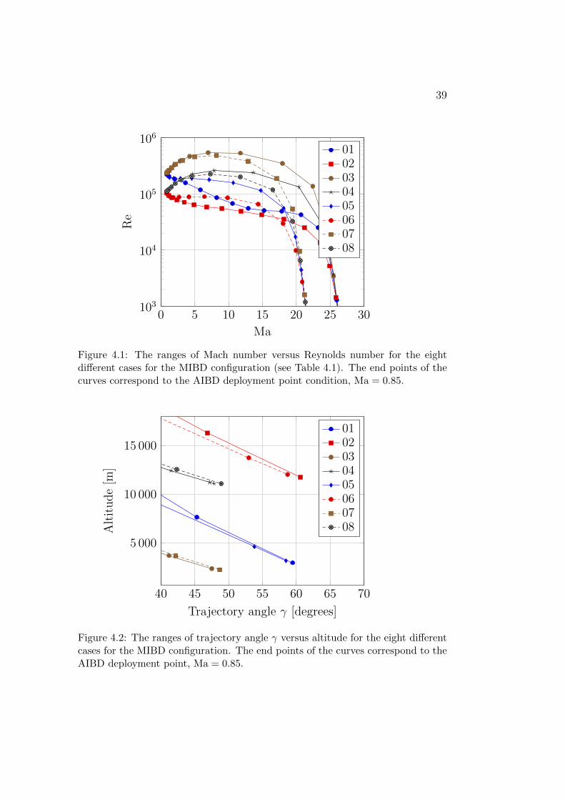
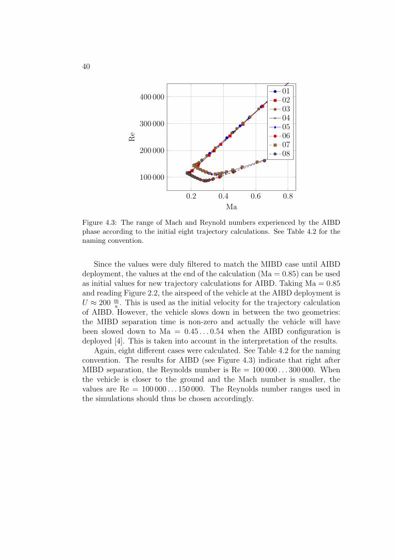
With these initial values and the atmospheric model provided in Section2.2, eight different trajectories are calculated for the MIBD phase. See Ta-ble 4.1 for the naming convention. The results were filtered so that Kn < 0.2and Ma ≥ 0.85. The following conclusions are drawn from the results for theMIBD phase:

• The possible Reynolds number values are Re = 40 000 . . . 500 000, ap-plicable to almost the whole range of Mach numbers. However, at verylarge Mach numbers, Reynolds number becomes very small, that isRe ≈ 200 when Ma & 25.

• The Reynolds number achieved at the end of the MIBD phase (Ma =0.85) are Re = 100 000 . . . 300 000.

• The altitude at which Ma = 0.85 is achieved is in the range 2 . . . 12 km.The lower value is alarming, but it is achieved when CD = 0.6, whichis a very small value for the drag coefficient. Once the simulated valuefor the drag coefficient is known, a better trajectory calculation can bemade.

• The trajectory angle at Ma = 0.85 is γ ≈ 50◦ . . . 60◦.

39

0 5 10 15 20 25 30103

104

105

106

Ma

Re

0102030405060708

Figure 4.1: The ranges of Mach number versus Reynolds number for the eightdifferent cases for the MIBD configuration (see Table 4.1). The end points of thecurves correspond to the AIBD deployment point condition, Ma = 0.85.

40 45 50 55 60 65 70

5 000

10 000

15 000

Trajectory angle γ [degrees]

Alt

itude

[m]

0102030405060708

Figure 4.2: The ranges of trajectory angle γ versus altitude for the eight differentcases for the MIBD configuration. The end points of the curves correspond to theAIBD deployment point, Ma = 0.85.

40

0.2 0.4 0.6 0.8

100 000

200 000

300 000

400 000

Ma

Re

0102030405060708

Figure 4.3: The range of Mach and Reynold numbers experienced by the AIBDphase according to the initial eight trajectory calculations. See Table 4.2 for thenaming convention.

Since the values were duly filtered to match the MIBD case until AIBDdeployment, the values at the end of the calculation (Ma = 0.85) can be usedas initial values for new trajectory calculations for AIBD. Taking Ma = 0.85and reading Figure 2.2, the airspeed of the vehicle at the AIBD deployment isU ≈ 200 m

s. This is used as the initial velocity for the trajectory calculation

of AIBD. However, the vehicle slows down in between the two geometries:the MIBD separation time is non-zero and actually the vehicle will havebeen slowed down to Ma = 0.45 . . . 0.54 when the AIBD configuration isdeployed [4]. This is taken into account in the interpretation of the results.

Again, eight different cases were calculated. See Table 4.2 for the namingconvention. The results for AIBD (see Figure 4.3) indicate that right afterMIBD separation, the Reynolds number is Re = 100 000 . . . 300 000. Whenthe vehicle is closer to the ground and the Mach number is smaller, thevalues are Re = 100 000 . . . 150 000. The Reynolds number ranges used inthe simulations should thus be chosen accordingly.

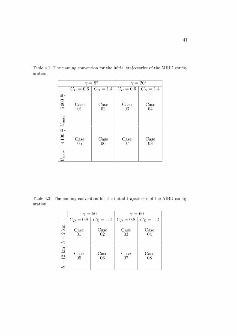
41

Table 4.1: The naming convention for the initial trajectories of the MIBD config-uration.

γ = 8◦ γ = 20◦

CD = 0.6 CD = 1.4 CD = 0.6 CD = 1.4

Uen

try

=5

000

m s

Case01

Case02

Case03

Case04

Uen

try

=4

100

m s

Case05

Case06

Case07

Case08

Table 4.2: The naming convention for the initial trajectories of the AIBD config-uration.

γ = 50◦ γ = 60◦

CD = 0.8 CD = 1.2 CD = 0.8 CD = 1.2

h=

2km

Case01

Case02

Case03

Case04

h=

12km

Case05

Case06

Case07

Case08

42

4.2 Minimum entry angle for the atmospheric

entry

If the entry angle is very small, it is possible that the vehicle bounces backto space and does not land on the planet at all. Therefore we define theminimum entry angle or the smallest entry angle γinit whereby the vehiclereaches the ground. Heat loads could also impose limits for the entry angle,but in this portion we are only treating the trajectory calculations.

The code already developed for the trajectory calculations can be directlyused to look for the minimum entry angle. It is not possible to formulate ananalytical expression for the angle, since none of the Equations (4.1) directlycorresponds to this case. Interpreting the trajectory equations, the causefor this is the combination of flight velocity and altitude. Since they cannotbe directly connected with an equation, we must manage with numericalcalculations. Due to the nature of the phenomenon, it is easy to implement acondition for this event: we simply stipulate that should the vehicle’s altitudeever surpass the initial altitude, then it is considered as bounced back.

The starting point of these calculations is the ensemble of initial valuesalready set in Section 4.1. It was observed that the minimum entry angleis virtually independent of the initial altitude and velocity, as long as theyremain in the same order of magnitude as normally in the project (initialaltitude hinit = 120 km, initial velocity Uinit = 4586 m

s). The only remain-

ing value to be defined is the ballistic coefficient (in the traditional sense,where mass is used instead of weight). Let us denote this traditional ballisticcoefficient by

βm =m

CDS(4.4)

The results from LA indicate that this value could be approximatelyβm ≈ 19 . . . 22 for the MetNet lander. It is now possible to calculate theminimum entry angles when the value of βm is set. The results are in Ta-ble 4.3. For the MetNet case, it would be, therefore, sensible to limit theentry angle to angles greater than 6 degrees.

Table 4.3: The minimum entry angles to prevent bounce-back, for the MetNetcase as a function of the traditional ballistic coefficient.

βm 8 15 20 30 45 70 100 150 200Minimum

entry angleγmin, degrees 5.25 5.65 5.83 6.07 6.31 6.55 6.75 6.96 7.11

43

Chapter 5

FINFLO Solver

5.1 Solution algorithm

In order to solve the quantities in the flow field, the so called Reynoldsaveraging process is used [28], where each quantity is decomposed into thetime averaged part and the fluctuating part. Any flow quantity Q is thenwritten as

Q(x, y, z, t) = Q(x, y, z) +Q′(x, y, z, t) (5.1)

where Q(x, y, z) is the time averaged part and Q′(x, y, z, t) is the fluctuating

part. When this technique is applied to the Navier-Stokes equations, the socalled Reynolds-averaged Navier Stokes (RANS) equations are formed. Theseare the equations that FINFLO solves, and the FINFLO manual formulatesthis equation as [24]

∂U

∂t+∂ (Fi − Fvi)

∂ui= Qs (5.2)

where U = (ρ, ρu1, ρu2, ρu3, E, ρk, ρε, ρφ)T and Qs is the source term. Ein-stein summation over i is implied in this equation. The terms ui representthe flow velocities so that ~U = u1

~i+u2~j+u3

~k. The inviscid and viscid fluxesare solved separately, and the inviscid fluxes are solved with Roe’s flux dif-ference splitting method. This can be also modified by the user. The inviscidterms Fi are

44

Fi =

ρuiρu1ui + δi,1

(p+ 2

3ρk)

ρu2ui + δi,2(p+ 2

3ρk)

ρu3ui + δi,3(p+ 2

3ρk)

(E + p+ 23ρk)ui

ρuikρuiερuiφ

(5.3)

where E is the total internal energy, ε is turbulent dissipation, and φ is “ascalar variable describing, eg. the concentration of a species or the massfraction of species”. The viscous fluxes in Equation (5.2) are

Fvi =

0τ1i

τ2i

τ3i

ujτij − qiµk (∂k/∂xi)µε (∂ε/∂xi)µφ (∂φ/∂xi)

(5.4)

where the Reynolds stress tensor components τi,j are defined in Equation (3.2),qi are the heat fluxes, and µk, µε and µφ are the diffusion coefficients of tur-bulence. The Einstein summation over j is implied in Equation (5.4).

Equation (5.2) can be solved numerically when the solution domain isdiscretised with the generated calculation mesh. There are several optionsfor the numerical derivative discretisation scheme, including the first-orderupwind, central, and second-order upwind schemes. The derivative termsare thus approximated as constants in each cell. Once the finite-volumetechnique is applied, Equation (5.2) can be integrated over the volumes andsurfaces, and the Gaussian divergence theorem yields the following equationfor a computational cell i:

VidUidt

=∑faces

(−ScellF + ViQi

)(5.5)

where Vi is the volume of the computation cell, F = njFj is the flux througha face, nj are the surface unit normals, Scell is the surface area, and Qi isthe flux term in the cell. After this phase, the equations are rearranged in amatrix form so that

[System matrix] {∆(Quantities)} = {Residuals} (5.6)

45

If a density-based solution method is used in FINFLO, the DADI factori-sation is applied to the system matrix. The residuals in the equation repre-sent the implicit part of the system of equations, and therefore iteration ofthese equations has to be carried out. In the previous equation, ∆ representsthe change of quantities between iteration cycles. All the quantities can beconsidered solved if they change very little between iteration cycles. In otherwords, it is desirable that the residuals diminish as the number of iterationcycles grows. It is also possible to follow the evolution of residuals in realtime during the calculation by calculating the L2 (Eucledian) norm of theresidual quantity in the Convergence program. See Figure 5.1 for an examplegraph of this evolution.

10000 20000 30000 40000

CYCLES

10-9

10-8

10-7

10-6

||||

2

Convergence history

MetNet Lander, uusi hila -Free stream Mach number 0.800Reynolds number 2.00 5Angle of attack 0.00 degreesfi le: /wrk17/mpalin/MIBU-General/MIBU-August-ReferenssitUusiks/IBDIAG

Date and time: Sept 09, 2015 09:58:58

Figure 5.1: An example of residual diminuation for the MIBD case in a FINFLOsimulation. The angle of attack was changed every 5 000 iterations, resulting inconvergence between the different angles of attack. The graph was created withthe FINFLO tool Convergence.

46

5.2 Turbulence model

When the Reynolds averaging process, discussed in the previous section, iscarried out, terms called the Reynolds stresses (written as u

′′i u

′′j ) occur in the

equations. These terms can be thought as the turbulence terms and theyneed to be modelled.

The turbulence model of choice in this work is the Shear-Stress Trans-port (SST) k-ω-model, which belongs to the class of two-equation turbulenceenergy equation models. The idea behind the chosen model is to predict tur-bulence by introducing two parameters, k (turbulence kinetic energy) and ω(specific rate of dissipation of the turbulence kinetic energy), and then solvingtwo partial differential equations for them [29]. This model has well provenits capabilities in the past decades and it can be thought as a combination ofthe k-ε and k-ω-models. This is because the latter is used in the boundarylayers and the former in the free stream zones [30]. In order to ensure propermodel selection, a blending function is used which operates as a functionof the distance from the nearest wall. In FINFLO, two boundary conditionvalues need to be specified by the user, which are the minimum value for ωand the free stream value of k. Also, the dimensionless turbulent viscositycan be limited with a maximum value. With these closure coefficients, theiteration cycle can be initiated.

The two equations are traditionally written as follows:∂(ρk)

∂t+∂(ρujk)

∂xj= P − β∗ρωk + ∂

∂xj

[(µ+ σkµT ) ∂k

∂xj

]∂(ρω)

∂t+∂(ρujω)

∂xj= γ ρ

µTP − βρω2 + ∂

∂xj

[(µ+ σωµT ) ∂ω

∂xj

]+2(1− F1)ρσω2

ω∂k∂xj

∂ω∂xj

, (5.7)

where P is the production of kinetic energy, defined by

P = ρu′′i u

′′j

∂ui∂xj

(5.8)

µT is the turbulent eddy viscosity, calculated from

µT =ρa1k

max (a1ω, SF2)(5.9)

and the constant values can be seen in Table 5.1. The auxiliary coefficientsγ1 and γ2 are

γ1 =β1

β∗− σω1k

2

√β∗

γ2 =β2

β∗− σω2k

2

√β∗

(5.10)

47

Table 5.1: Coefficient values in the SST k-ω turbulence model [31].

Coefficient β∗ σk1 σk2 σω1 σω2 β1 β2 a1

Value 0.09 0.44 1 0.85 0.856 0.5 0.0828 0.31

The blending functions areF1 = tanh

[

min

(max

( √k

β∗ωy,500µ

ρy2ω

),

4ρσω2k

CDkωy2

)]4

F2 = tanh

[

max

(2

√k

β∗ωy,500µ

ρy2ω

)]2

(5.11)

where

CDkω = max

(2ρσω2

ω

∂k

∂xi

∂ω

∂xi, 10−10

)(5.12)

The term S is related to the mean strain-rate tensor:

S =√si,jsj,i where si,j =

1

2

(∂ui∂uj

+∂uj∂xi

)(5.13)

Finally, the Reynolds stresses are calculated with the Boussinesq approx-imation [24] (compare with Equation 3.2)

− ρu′′i u

′′j = µT

[∂uj∂xi

+∂ui∂xj− 2

3

∂uk∂xk

δi,j

]− 2

3ρkδi,j (5.14)

48

49

Chapter 6

Simulations

6.1 Simulation setup

6.1.1 Mesh Resolution

In order to correctly build the grid for the cases to be simulated, we need tofirst calculate the requirement for the height of the first mesh cell, here to bedenoted by ∆s, required to achieve a desired y+, the dimensionless distancefrom the wall, using flat-plate boundary layer theory. The condition for thisis

∆s =y+µ

Uτρ(6.1)

The friction velocity, here denoted by Uτ , for a wall can be calculated from [32]

Uτ =

√τwall

ρ, (6.2)

where τwall is the wall shear stress. It can be calculated as

τwall = cf1

2ρU2 (6.3)

Here U is the free stream velocity and cf is the friction coefficient. White [32]provides an approximation for the friction coefficient for the case of a turbu-lent boundary layer:

cf ≈0.027

Re1/7x

(6.4)

Here Rex is the Reynolds number referred to the distance from the leadingedge in the case of an airfoil. We can adopt this to our case by setting x

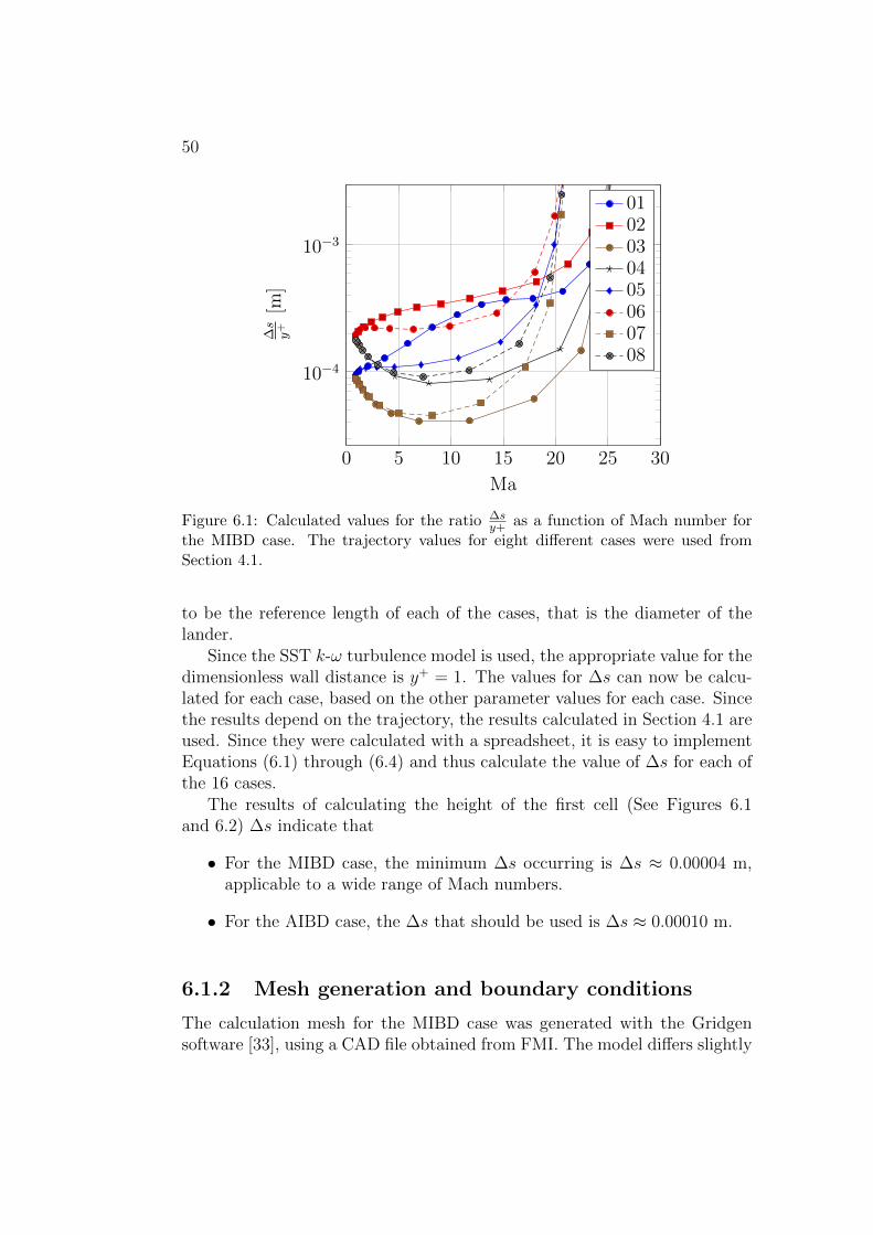
50

0 5 10 15 20 25 30

10−4

10−3

Ma

∆s

y+

[m]

0102030405060708

Figure 6.1: Calculated values for the ratio ∆sy+ as a function of Mach number for

the MIBD case. The trajectory values for eight different cases were used fromSection 4.1.

to be the reference length of each of the cases, that is the diameter of thelander.

Since the SST k-ω turbulence model is used, the appropriate value for thedimensionless wall distance is y+ = 1. The values for ∆s can now be calcu-lated for each case, based on the other parameter values for each case. Sincethe results depend on the trajectory, the results calculated in Section 4.1 areused. Since they were calculated with a spreadsheet, it is easy to implementEquations (6.1) through (6.4) and thus calculate the value of ∆s for each ofthe 16 cases.

The results of calculating the height of the first cell (See Figures 6.1and 6.2) ∆s indicate that

• For the MIBD case, the minimum ∆s occurring is ∆s ≈ 0.00004 m,applicable to a wide range of Mach numbers.

• For the AIBD case, the ∆s that should be used is ∆s ≈ 0.00010 m.

6.1.2 Mesh generation and boundary conditions

The calculation mesh for the MIBD case was generated with the Gridgensoftware [33], using a CAD file obtained from FMI. The model differs slightly

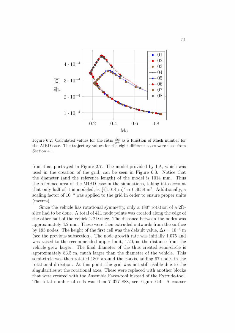
51

0.2 0.4 0.6 0.8

1 · 10−4

2 · 10−4

3 · 10−4

4 · 10−4

Ma

∆s

y+

[m]

0102030405060708

Figure 6.2: Calculated values for the ratio ∆sy+ as a function of Mach number for

the AIBD case. The trajectory values for the eight different cases were used fromSection 4.1.

from that portrayed in Figure 2.7. The model provided by LA, which wasused in the creation of the grid, can be seen in Figure 6.3. Notice thatthe diameter (and the reference length) of the model is 1014 mm. Thusthe reference area of the MIBD case in the simulations, taking into accountthat only half of it is modeled, is π

8(1.014 m)2 ≈ 0.4038 m2. Additionally, a

scaling factor of 10−3 was applied to the grid in order to ensure proper units(metres).

Since the vehicle has rotational symmetry, only a 180◦ rotation of a 2D-slice had to be done. A total of 411 node points was created along the edge ofthe other half of the vehicle’s 2D slice. The distance between the nodes wasapproximately 4.2 mm. These were then extruded outwards from the surfaceby 193 nodes. The height of the first cell was the default value, ∆s = 10−5 m(see the previous subsection). The node growth rate was initially 1.075 andwas raised to the recommended upper limit, 1.20, as the distance from thevehicle grew larger. The final diameter of the thus created semi-circle isapproximately 83.5 m, much larger than the diameter of the vehicle. Thissemi-circle was then rotated 180◦ around the x-axis, adding 97 nodes in therotational direction. At this point, the grid was not still usable due to thesingularities at the rotational axes. These were replaced with another blocksthat were created with the Assemble Faces-tool instead of the Extrude-tool.The total number of cells was then 7 077 888, see Figure 6.4. A coarser

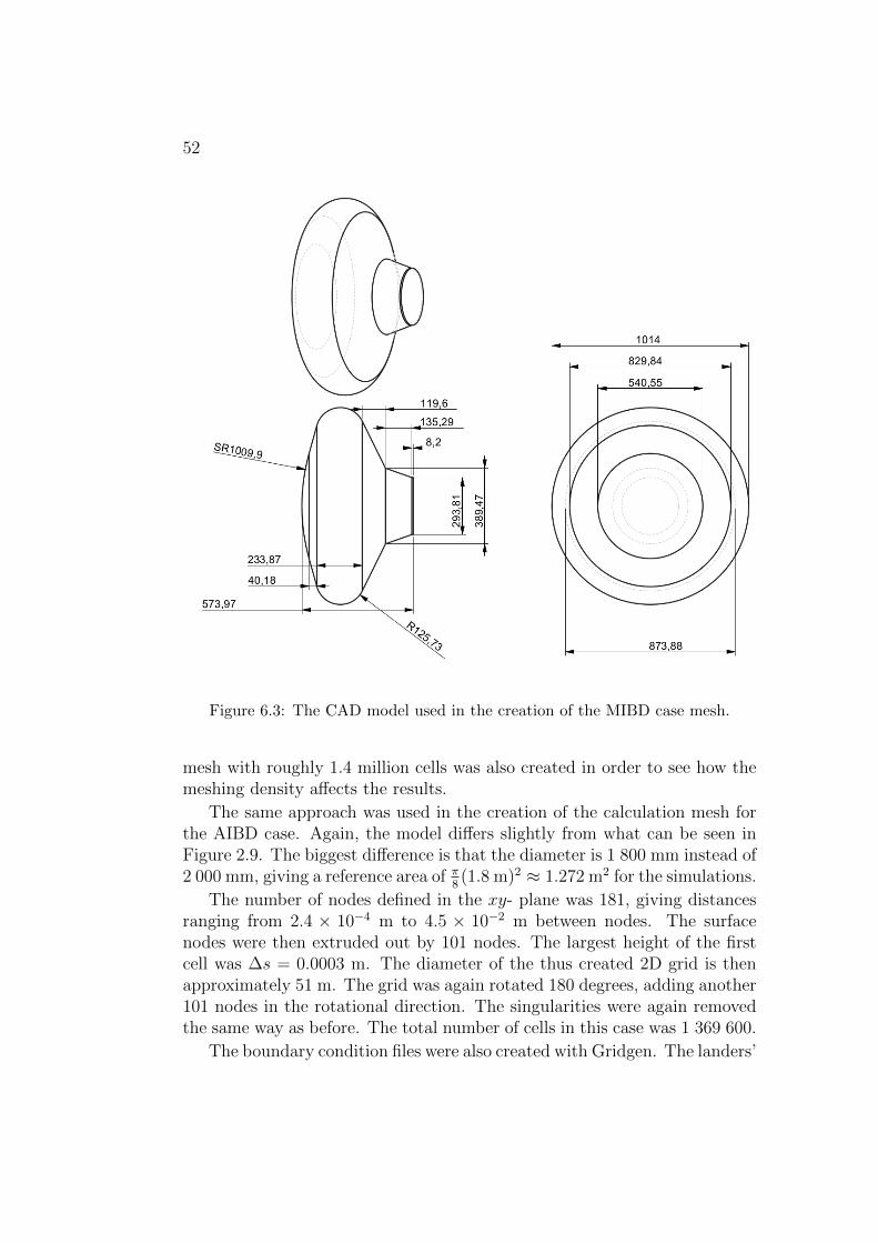
52

Figure 6.3: The CAD model used in the creation of the MIBD case mesh.

mesh with roughly 1.4 million cells was also created in order to see how themeshing density affects the results.

The same approach was used in the creation of the calculation mesh forthe AIBD case. Again, the model differs slightly from what can be seen inFigure 2.9. The biggest difference is that the diameter is 1 800 mm instead of2 000 mm, giving a reference area of π

8(1.8 m)2 ≈ 1.272 m2 for the simulations.

The number of nodes defined in the xy- plane was 181, giving distancesranging from 2.4 × 10−4 m to 4.5 × 10−2 m between nodes. The surfacenodes were then extruded out by 101 nodes. The largest height of the firstcell was ∆s = 0.0003 m. The diameter of the thus created 2D grid is thenapproximately 51 m. The grid was again rotated 180 degrees, adding another101 nodes in the rotational direction. The singularities were again removedthe same way as before. The total number of cells in this case was 1 369 600.

The boundary condition files were also created with Gridgen. The landers’

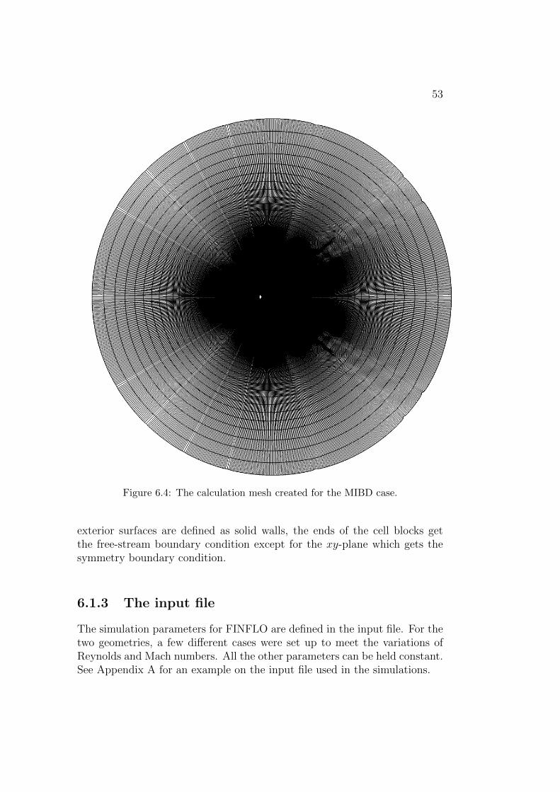
53

Figure 6.4: The calculation mesh created for the MIBD case.

exterior surfaces are defined as solid walls, the ends of the cell blocks getthe free-stream boundary condition except for the xy-plane which gets thesymmetry boundary condition.

6.1.3 The input file

The simulation parameters for FINFLO are defined in the input file. For thetwo geometries, a few different cases were set up to meet the variations ofReynolds and Mach numbers. All the other parameters can be held constant.See Appendix A for an example on the input file used in the simulations.

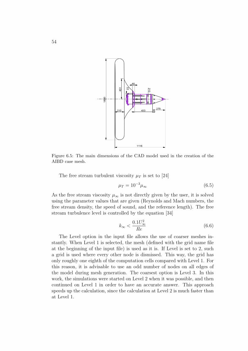
54

Figure 6.5: The main dimensions of the CAD model used in the creation of theAIBD case mesh.

The free stream turbulent viscosity µT is set to [24]

µT = 10−3µ∞ (6.5)

As the free stream viscosity µ∞ is not directly given by the user, it is solvedusing the parameter values that are given (Reynolds and Mach numbers, thefree stream density, the speed of sound, and the reference length). The freestream turbulence level is controlled by the equation [34]

k∞ <0.1U2

∞Re

(6.6)

The Level option in the input file allows the use of coarser meshes in-stantly. When Level 1 is selected, the mesh (defined with the grid name fileat the beginning of the input file) is used as it is. If Level is set to 2, sucha grid is used where every other node is dismissed. This way, the grid hasonly roughly one eighth of the computation cells compared with Level 1. Forthis reason, it is advisable to use an odd number of nodes on all edges ofthe model during mesh generation. The coarsest option is Level 3. In thiswork, the simulations were started on Level 2 when it was possible, and thencontinued on Level 1 in order to have an accurate answer. This approachspeeds up the calculation, since the calculation at Level 2 is much faster thanat Level 1.

55

As noted in Section 5.1, Roe’s flux splitting method was employed andfull friction terms were turned off in the equations with FULLNC = ’NO’.This again speeds up the calculation but, in practise, does not impair theresults. Additionally, this choice was recommended in the manual. Tur-bulence correction at walls was also turned on [35]. As for the derivativediscretisation, the simulations were initiated with first-order upwind method(at Level 2) and when that was converged, the more accurate second-orderupwind method was continued (at Level 1).

The Courant number is defined as

Cn =u∆t

∆x(6.7)

where u is the local velocity in a computation cell, ∆t is the time step and ∆xis a measure of the size of the computation cell. Even though time-averagedcomputation is used, it is still necessary to define a value for this number.Since implicit methods are used, it does not impose any stability limits for thesimulation, and, therefore, its value can be chosen relatively freely. In practiseit was noted that increasing the value increased the oscillation amplitudesat first, but the simulation converged faster. This way, choosing the rightCourant number is always a compromise.

6.2 Simulations and results

6.2.1 MetNet DV with inflated MIBD

Each case with different angles of attack was simulated 5 000 iterations. Theaerodynamic coefficients for the cases were then obtained by interpreting theresults with the Convergence program. The program can draw graphs of thecoefficients as a function of the iteration number. The values oscillate as afunction of the iteration cycle, but the amplitudes diminish as the calculationprogresses. This, along with the decrease of the residuals, was interpreted asthe convergence of the calculation. After the mentioned 5 000 iterations, theabsolute error (or: the amplitude of oscillation) of the aerodynamic coeffi-cients had decreased to, for the majority of the cases, below ±0.005 counts.See Figure 6.6 for an example graph and how the result was interpreted. Thecalculation time with the coarser grid for each case (with a fixed angle of at-tack) was of the order of two hours when 10 cores were used in the computer(Intel R© Xeon R© CPU E5-1650 v2, 3.50GHz).

Unfortunately, the maximum Mach number that was achieved in thesimulations was Ma = 1.9. Even with this value, the iteration errors in the

56

values would grow considerably and at larger values the simulation wouldno longer converge. This was observed by following the growth of residualsduring the simulation with the Convergence program. Thus the set of Machnumbers used for the MIBD case were Ma = 0.8, Ma = 1.3, Ma = 1.7 andMa = 1.9.

A graph of the result for the drag coefficient can be found in Figure B.1.The conclusions that can be drawn from these results are the following:

• The effect of the Reynolds number on the drag coefficient is minimaland often within error limits. This can be seen by comparing the casesRe = 40 000 and Re = 500 000.

• The drag coefficient grows with increasing Mach number. This can beseen also in the values provided by LA, but since only four cases weresimulated, it is not reasonable to calculate any approximations for thedrag coefficient’s evolution with the Mach number.

• While the results for large Mach numbers and small angles of attackagree well with the results from LA, there are apparent differencesbetween the other results. The drag coefficients for subsonic speeds,calculated by FINFLO are some 10 % smaller than those obtained fromthe calculations by LA. It is difficult to estimate any sources for thisreason due to the lack of documentation concerning the results by LA.

A graph of the result for the lift coefficient is in Figure B.2. The valuesare generally in fairly good agreement with the results from LA although thedifferences increase at the larger angles of attack. Another observation thatcan be made is that the lift slope CLα grows (in the sense of absolute value) asa function of the Mach number, but there is no noticeable difference betweenthe cases Ma = 1.3 and Ma = 1.9, in which case the slope is approximatelyCLα ≈ −0.9 1

rad.

The most interesting result and the primary goal of this work is the setof values obtained for the pitching moment coefficient. These are drawnin Figure B.3. Even though there are, again, clear differences between theresults, the tendency is clear: The slope of the pitching moment is nega-tive. This indicates static stability for the vehicle in the simulated cases (seeSection 3.2).

6.2.2 Penetrating part after the separation of the frontshield (AIBD case)

Following the results from Section 4.1, three different cases were set up:

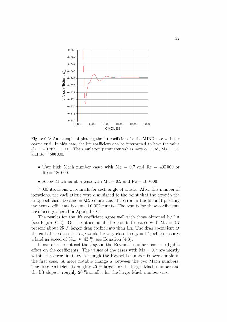
57

15000. 16000. 17000. 18000. 19000. 20000.

CYCLES

-0.280

-0.278

-0.276

-0.274

-0.272

-0.270

-0.268

-0.266

-0.264

-0.262

-0.260

Lif

t co

eff

icie

nt

Convergence history

MetNet Lander, uusi hila -Free stream Mach number 1.300Reynolds number 5.00 5Angle of attack 0.00 degreesfi le: /wrk17/mpalin/MIBU-General/MIBU-August-ReferenssitUusiks/IBDIAG

Date and time: Sept 07, 2015 10:09:05

Figure 6.6: An example of plotting the lift coefficient for the MIBD case with thecoarse grid. In this case, the lift coefficient can be interpreted to have the valueCL = −0.267 ± 0.001. The simulation parameter values were α = 15◦, Ma = 1.3,and Re = 500 000.

• Two high Mach number cases with Ma = 0.7 and Re = 400 000 orRe = 180 000.

• A low Mach number case with Ma = 0.2 and Re = 100 000.

7 000 iterations were made for each angle of attack. After this number ofiterations, the oscillations were diminished to the point that the error in thedrag coefficient became ±0.02 counts and the error in the lift and pitchingmoment coefficients became ±0.002 counts. The results for these coefficientshave been gathered in Appendix C.

The results for the lift coefficient agree well with those obtained by LA(see Figure C.2). On the other hand, the results for cases with Ma = 0.7present about 25 % larger drag coefficients than LA. The drag coefficient atthe end of the descent stage would be very close to CD = 1.1, which ensuresa landing speed of Ufinal ≈ 43 m

s, see Equation (4.3).

It can also be noticed that, again, the Reynolds number has a negligibleeffect on the coefficients. The values of the cases with Ma = 0.7 are mostlywithin the error limits even though the Reynolds number is over double inthe first case. A more notable change is between the two Mach numbers.The drag coefficient is roughly 20 % larger for the larger Mach number andthe lift slope is roughly 20 % smaller for the larger Mach number case.

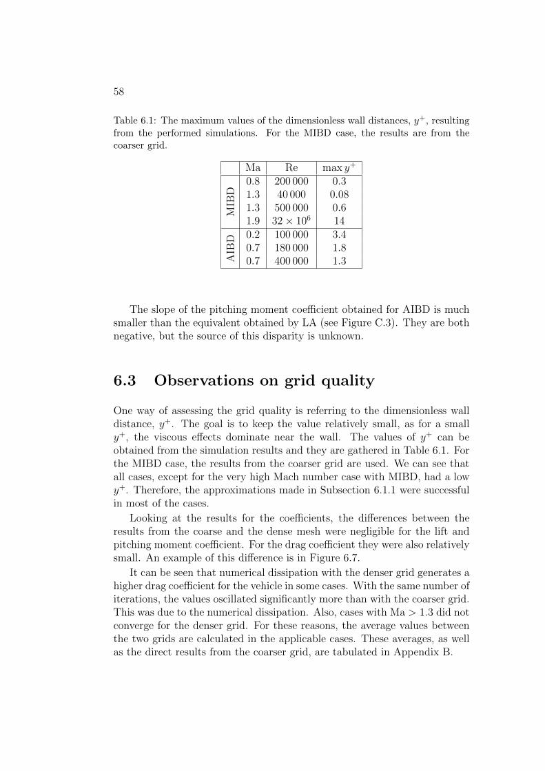
58

Table 6.1: The maximum values of the dimensionless wall distances, y+, resultingfrom the performed simulations. For the MIBD case, the results are from thecoarser grid.

Ma Re max y+

MIB

D

0.8 200 000 0.31.3 40 000 0.081.3 500 000 0.61.9 32× 106 14

AIB

D 0.2 100 000 3.40.7 180 000 1.80.7 400 000 1.3

The slope of the pitching moment coefficient obtained for AIBD is muchsmaller than the equivalent obtained by LA (see Figure C.3). They are bothnegative, but the source of this disparity is unknown.

6.3 Observations on grid quality

One way of assessing the grid quality is referring to the dimensionless walldistance, y+. The goal is to keep the value relatively small, as for a smally+, the viscous effects dominate near the wall. The values of y+ can beobtained from the simulation results and they are gathered in Table 6.1. Forthe MIBD case, the results from the coarser grid are used. We can see thatall cases, except for the very high Mach number case with MIBD, had a lowy+. Therefore, the approximations made in Subsection 6.1.1 were successfulin most of the cases.

Looking at the results for the coefficients, the differences between theresults from the coarse and the dense mesh were negligible for the lift andpitching moment coefficient. For the drag coefficient they were also relativelysmall. An example of this difference is in Figure 6.7.

It can be seen that numerical dissipation with the denser grid generates ahigher drag coefficient for the vehicle in some cases. With the same number ofiterations, the values oscillated significantly more than with the coarser grid.This was due to the numerical dissipation. Also, cases with Ma > 1.3 did notconverge for the denser grid. For these reasons, the average values betweenthe two grids are calculated in the applicable cases. These averages, as wellas the direct results from the coarser grid, are tabulated in Appendix B.

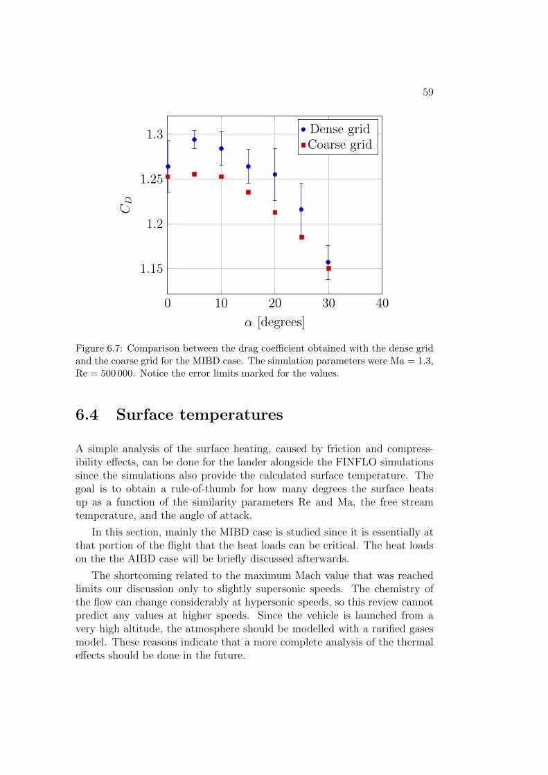
59

0 10 20 30 40

1.15

1.2

1.25

1.3

α [degrees]

CD

Dense gridCoarse grid

Figure 6.7: Comparison between the drag coefficient obtained with the dense gridand the coarse grid for the MIBD case. The simulation parameters were Ma = 1.3,Re = 500 000. Notice the error limits marked for the values.

6.4 Surface temperatures

A simple analysis of the surface heating, caused by friction and compress-ibility effects, can be done for the lander alongside the FINFLO simulationssince the simulations also provide the calculated surface temperature. Thegoal is to obtain a rule-of-thumb for how many degrees the surface heatsup as a function of the similarity parameters Re and Ma, the free streamtemperature, and the angle of attack.

In this section, mainly the MIBD case is studied since it is essentially atthat portion of the flight that the heat loads can be critical. The heat loadson the the AIBD case will be briefly discussed afterwards.

The shortcoming related to the maximum Mach value that was reachedlimits our discussion only to slightly supersonic speeds. The chemistry ofthe flow can change considerably at hypersonic speeds, so this review cannotpredict any values at higher speeds. Since the vehicle is launched from avery high altitude, the atmosphere should be modelled with a rarified gasesmodel. These reasons indicate that a more complete analysis of the thermaleffects should be done in the future.

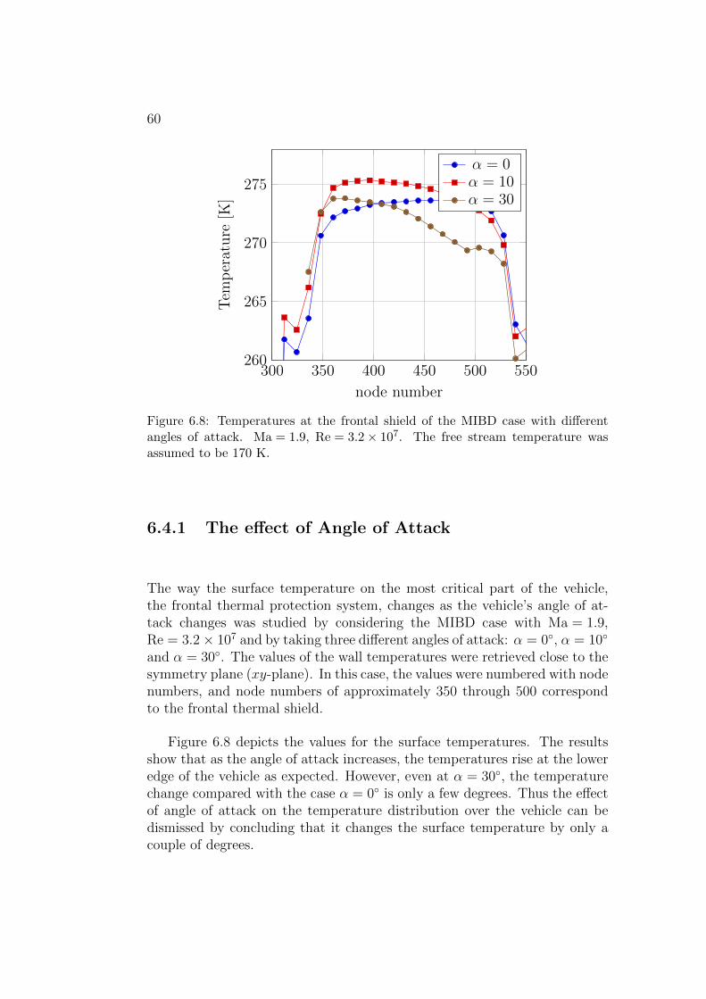
60

300 350 400 450 500 550260

265

270

275

node number

Tem

per

ature

[K]

α = 0α = 10α = 30

Figure 6.8: Temperatures at the frontal shield of the MIBD case with differentangles of attack. Ma = 1.9, Re = 3.2× 107. The free stream temperature wasassumed to be 170 K.

6.4.1 The effect of Angle of Attack

The way the surface temperature on the most critical part of the vehicle,the frontal thermal protection system, changes as the vehicle’s angle of at-tack changes was studied by considering the MIBD case with Ma = 1.9,Re = 3.2× 107 and by taking three different angles of attack: α = 0◦, α = 10◦

and α = 30◦. The values of the wall temperatures were retrieved close to thesymmetry plane (xy-plane). In this case, the values were numbered with nodenumbers, and node numbers of approximately 350 through 500 correspondto the frontal thermal shield.

Figure 6.8 depicts the values for the surface temperatures. The resultsshow that as the angle of attack increases, the temperatures rise at the loweredge of the vehicle as expected. However, even at α = 30◦, the temperaturechange compared with the case α = 0◦ is only a few degrees. Thus the effectof angle of attack on the temperature distribution over the vehicle can bedismissed by concluding that it changes the surface temperature by only acouple of degrees.

61

Table 6.2: Average surface temperature on the heat shield of the MIBD case asa function of the free stream temperature. The parameter values used for thesimulation were Ma = 1.3, Re = 500 000 and α = 35◦.

Free streamtemperature T∞ [K]

Average frontalsurface temperature T [K] T/T∞

140 183.62 1.31160 205.95 1.29180 231.48 1.29200 255.27 1.28220 281.27 1.28

6.4.2 The effect of free stream temperature

Similarly as in the previous subsection, the temperature of the thermal pro-tection system was studied as a function of the free stream temperature. Thistime, the MIBD case with Ma = 1.3, Re = 500 000 and α = 35◦ was studied.The range of the free stream temperatures was chosen to match the valuesthat the vehicle might experience during the descent phase (see Figure 2.4).The average values of wall temperatures corresponding to the frontal heatshield were calculated for each case and the results are in Table 6.2.

The regression for the values shows that an increase of 10 K in the freestream temperature raises the surface temperature by approximately 12.2 K.This cannot, however, fully predict the surface temperatures since it is alsodependent of other parameters. Nevertheless, this is a useful value that canbe used to estimate changes in the temperature.

6.4.3 The effect of the Reynolds number

For the case of the MIBD configuration at Ma = 1.3, two different cases withlargely different Reynolds numbers were calculated earlier. The surface tem-peratures can now be compared in order to assess the effect of the Reynoldsnumber in this case. Statistics of the wall temperatures have been gatheredin Table 6.3. The points were again gathered to correspond to the most crit-ical part of the vehicle, nodes 350 through 500. As can be easily seen, thedifference in the mean temperature is very small. Also, a simple two-meanZ-test gives a p-value of p ≈ 0.215, confirming that the two means are notsignificantly different. Thus it can be concluded that the Reynolds numberhas virtually no effect on the surface temperature.

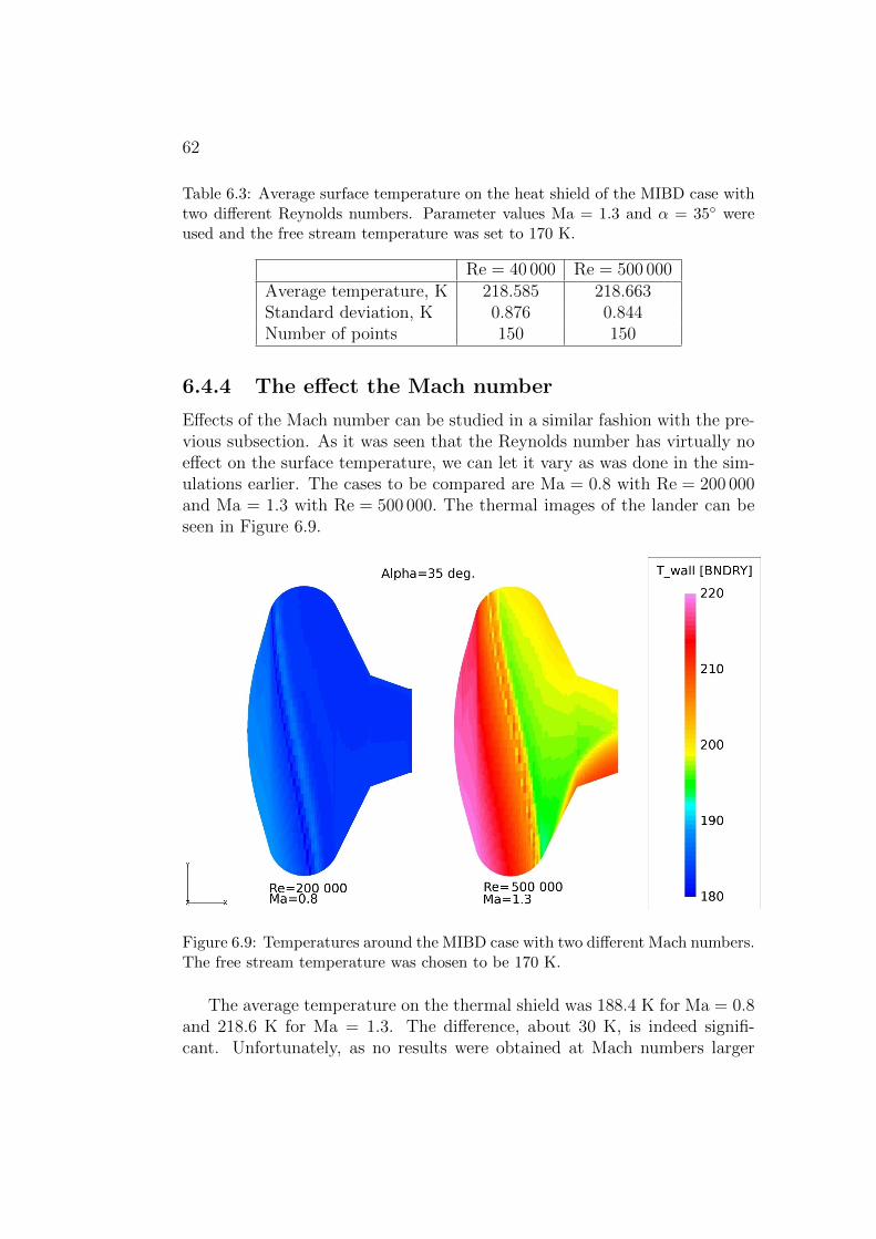
62

Table 6.3: Average surface temperature on the heat shield of the MIBD case withtwo different Reynolds numbers. Parameter values Ma = 1.3 and α = 35◦ wereused and the free stream temperature was set to 170 K.

Re = 40 000 Re = 500 000Average temperature, K 218.585 218.663Standard deviation, K 0.876 0.844Number of points 150 150

6.4.4 The effect the Mach number

Effects of the Mach number can be studied in a similar fashion with the pre-vious subsection. As it was seen that the Reynolds number has virtually noeffect on the surface temperature, we can let it vary as was done in the sim-ulations earlier. The cases to be compared are Ma = 0.8 with Re = 200 000and Ma = 1.3 with Re = 500 000. The thermal images of the lander can beseen in Figure 6.9.

Figure 6.9: Temperatures around the MIBD case with two different Mach numbers.The free stream temperature was chosen to be 170 K.

The average temperature on the thermal shield was 188.4 K for Ma = 0.8and 218.6 K for Ma = 1.3. The difference, about 30 K, is indeed signifi-cant. Unfortunately, as no results were obtained at Mach numbers larger

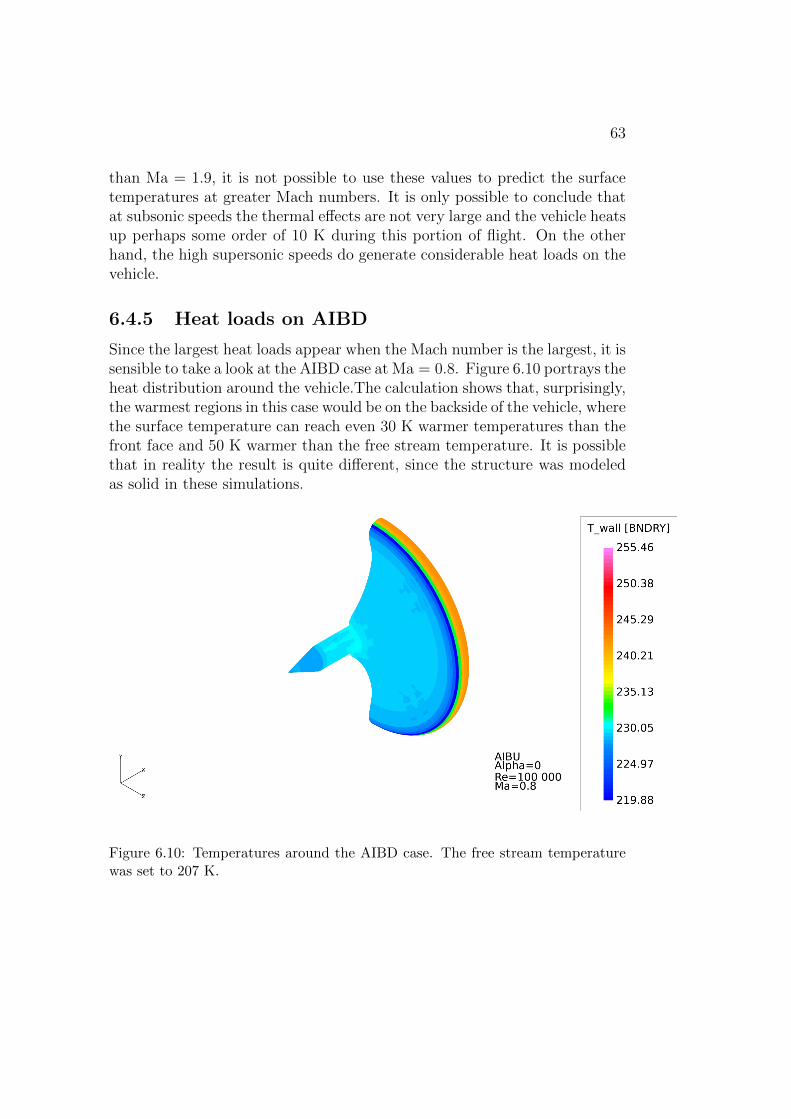
63

than Ma = 1.9, it is not possible to use these values to predict the surfacetemperatures at greater Mach numbers. It is only possible to conclude thatat subsonic speeds the thermal effects are not very large and the vehicle heatsup perhaps some order of 10 K during this portion of flight. On the otherhand, the high supersonic speeds do generate considerable heat loads on thevehicle.

6.4.5 Heat loads on AIBD

Since the largest heat loads appear when the Mach number is the largest, it issensible to take a look at the AIBD case at Ma = 0.8. Figure 6.10 portrays theheat distribution around the vehicle.The calculation shows that, surprisingly,the warmest regions in this case would be on the backside of the vehicle, wherethe surface temperature can reach even 30 K warmer temperatures than thefront face and 50 K warmer than the free stream temperature. It is possiblethat in reality the result is quite different, since the structure was modeledas solid in these simulations.

Figure 6.10: Temperatures around the AIBD case. The free stream temperaturewas set to 207 K.

64

65

Chapter 7

Conclusions and discussion

In this thesis, the aerodynamics of the Mars MetNet descent vehicle was ana-lysed by using the CFD software FINFLO by Aalto University. The MetNetEDLS has been developed in cooperation by the team comprising FMI, LA,and Instituto Nacional de Tecnica Aeroespacial with the responsibility ofaerodynamic design resting with LA. The simulations were set up to matchthe re-entry and descent conditions on Mars as closely as possible. In order tofacilitate the parameter selection, an atmospheric model was created in orderto approximately calculate the averages of temperature, density, the speedof sound, the specific heat ratio, and the dynamic viscosity as a function ofaltitude. The main source for these values was the Mars Climate Database.

A trajectory calculation code in Python was also developed with the ex-plicit first-order forward Euler method in order to calculate the combinationof Reynolds and Mach numbers that the vehicle experiences during the de-scent phase. The trajectory calculations provided a condition for the dimen-sionless wall distance y+ of the calculation mesh and therefore also helped inthe mesh generation. Two major MetNet geometries during the atmosphericentry trajectory, MIBD for the entry phase and AIBD for the descent phase,were modelled and simulated. Additionally, two different meshes were gen-erated for the former in order to assess the quality of the mesh.

The main goal of this work was to obtain the pertinent aerodynamic co-efficients and, therefore, to reinforce the results obtained by LA. The mostinteresting aerodynamic feature of the vehicle is the pitching moment coef-ficient Cm, a dimensionless measure of the tendency of the vehicle to rotatearound its centre of mass as a response to aerodynamic effects. Studyingthe values of this coefficient is essential in the analysis of the stability of thevehicle, since the slope of the pitching moment coefficient with respect to theangle of attack (see Section 3.1) determines the static stability of the vehicle.Dynamic stability, on the other hand, can be studied by calculating the slope

66

of this coefficient with respect to the pitch rate. Only the former of thesetwo is studied in this work due to extensive computations required by thelatter.

The drag coefficient CD, a measure of the air resistance generated by theflow around the vehicle, is another important quantity in the aerodynamicanalysis of the lander. It enables the computation of the deceleration duringthe re-entry and descent phase. The final impact speed is a function of thedrag coefficient and a large enough value is desired in order to ensure a safelanding for the vehicle. The drag coefficient, along with the other pertinentaerodynamic coefficients, is calculated with the FINFLO simulations in thiswork and then compared with the results by LA. The simulations also providesome insight to the temperature distributions around the vehicle and how itevolves as a function of different parameters.

The main contributions of this work are the atmospheric model, where theregressions are presented as equations that can be used later, the trajectorycode and the aerodynamic coefficients of the vehicle as a function of theangle of attack. These are the necessary tools in the aerodynamic analysisof the vehicle in its re-entry and descent phase. The results can be usedin future calculations that could include heat transfer analyses or dynamic(time-dependent) CFD simulations.

A major conclusion can be drawn from aerodynamic analysis using FIN-FLO simulations is that the MetNet Lander is statically stable at least upto Mach number 1.9. This result includes two points of caution. Firstly, theresult only encompasses the feature of static stability and not yet dynamicstability. On the other hand, the aerodynamic simulations and wind tunneltests performed by Lavochkin Association indicate that the MetNet landingvehicle would be also dynamically stable during the entry and descent phase.Secondly, the limitations of the code permitted converging simulations onlyup to the mentioned Mach number. The slope of the pitching moment coeffi-cient was negative for all these simulations, which is a promising result, but itis difficult to estimate how this value would evolve at hypersonic speeds. Theearlier simulations by LA show strong nonlinear behaviour of Cm for higherspeeds, and hence proper simulations with higher Mach numbers should becarried out. A specialised rarified gases code or a hypersonic model with arefined gas chemistry model should be used for such simulations.

The numerical values of the lift coefficient are in fairly good agreementwith the earlier results by the LA, especially during the AIBD phase. Thisaspect serves as evidence for the validity of the results. On the other hand,other aerodynamic coefficients exhibit more deviations with the earlier ana-lyses. For example, our results for the drag coefficient present noticeable dif-ferences between LA’s results almost across the board. However, the change

67

is in a positive direction, as a large drag coefficient is specifically desired.Finally, the thermal results point out that the most drastic heating of the

vehicle develops at supersonic speeds as expected. For this reason, mainlythe MIBD state is subject to heating. The parameters determining the sur-face temperature are shown to be the Mach number and the free streamtemperature, while the Reynolds number and the angle of attack (assumingthat they stay within certain limits) have a practically negligible effect.

The analyses of this thesis suggest that the Mars MetNet vehicle is stat-ically stable during the entry and descent trajectory phases during its land-ing on Mars through the Martian atmosphere. The conclusions are similarto those gained by the earlier work by the MetNet development team. Themodelling and simulations included various simplifications and idealisationsthat should be taken into account when making MetNet system and mis-sions decisions. Additional modelling and simulation work are recommendedto confirm the thesis results. Furthermore, additional aerodynamic simula-tions and wind tunnel tests will facilitate the extension of the thesis resultssuch that they will contribute to the dynamic stability analysis of the MetNetvehicle.

68

69

Bibliography

[1] NASA & California Institute of Technology, “Mars explorationrovers,” http://mars.nasa.gov/mer/mission/spacecraft_edl.html. Re-trieved February 2nd, 2015.

[2] NASA & California Institute of Technology, “Mars explorationrover,” http://www.jpl.nasa.gov/news/fact_sheets/mars03rovers.

pdf. Retrieved February 3rd, 2015.

[3] Finnish Meteorological Institute, “Mars MetNet Mission,” http://

metnet.fmi.fi/index.php. Retrieved February 3rd, 2015.

[4] A.-M. Harri, “RITD final report,” technical report, February 24th 2015.

[5] Russian Aviation and Space Agency, “Project documentation for se-lected concept,” technical report, April 17th 2002.

[6] A-M. Harri, S. Alexashin et al., “Mars MetNet Mission Sta-tus,” http://www.researchgate.net/publication/282274917_Mars_

MetNet_Mission_Status. Retrieved October 5th 2015.

[7] A. Hellsten, K. Kaarlonen, J. Saloranta et al., “Finflo-flow solver.” http:

//www.aero.hut.fi/Englanniksi/CFD_text/finflo__flow_solver.html.Retrieved February 3rd, 2015.

[8] Finnish Meteorological Institute, “Mars MetNet Mission,” http://

metnet.fmi.fi/index.php?id=93. Retrieved February 17th, 2015.

[9] A-M. Harri, P. Makkonen et al., “Martian Atmospheric Science Network- MetNet,” https://iafastro.directory/iac/archive/browse/IAC-04/

IAA.3.7/2/815/. Retrieved October 9th 2015.

[10] Lavochkin Association, “Scaling laws for Mars - Earth Re-entry Sys-tem,” technical report, December 24th 2012.

70

[11] Lavochkin Association, “Mathematical Model for projecting the windtunnel test results for Earth’s atmosphere,” technical report, December20th 2012.

[12] Lavochkin Association, “Test plan for the wind tunnel tests,” technicalreport, December 27th 2013.

[13] Lavochkin Association, “Test report of the wind tunnel tests,” technicalreport, July 28th 2014.

[14] Lavochkin Association, “Feasibility and design of EDLS system forEarth’s atmosphere,” technical report, December 27th 2014.

[15] Lavochkin Association, “Analysis of an inflatable EDLS’ dynamic sta-bility in the transsonic regime,” technical report, September 12th 2012.

[16] LMD, OU, IAA, ESA, CNES, “Mars Climate Database: The Web Inter-face,” http://www-mars.lmd.jussieu.fr/mcd_python/. Retrieved March6th 2015.

[17] F. Forget, E. Millour, and S. Lewis, “Mars Climate Database v5.1Detailed Design Document,” http://www-mars.lmd.jussieu.fr/mars/

info_web/MCD5.1_ddd.pdf. Retrieved March 3rd 2015.

[18] C. Justus, A. Duvall, and V. Keller, “Validation of Mars GlobalReference Atmospheric Model (Mars-GRAM 2001) and plannednew features,” http://www.sciencedirect.com/science/article/pii/

S0273117706004510. Retrieved March 9th 2015.

[19] A. Miettinen, E. Salminen, and T. Siikonen, “Kaksifaasivirtaussimuloin-timenetelmien kehitysta ja sovelluksia - Raportti 10,” Finflo Oy. Espoo2003.

[20] Lavochkin Association, “Feasibility of MetNet EDLS to Earth Re-entry,” technical report, December 27th 2011.

[21] Wikipedia, “Knudsen number,” https://en.wikipedia.org/wiki/

Knudsen_number. Retrieved July 16th 2015.

[22] Lavochkin Association, “Small (mini) landing station system tests,”technical report, December 10th 2012.

[23] Lavochkin Association, “Manufacturing of the MML’s experimentalmodels and ground-based test schedule,” technical report, July 27th2004.

71

[24] Finflo Ltd., FINFLO User Guide - Version 8.1. Espoo 2003.

[25] D. F. Kurtulus, F. Scarano, and L. David, “Unsteady aerodynamic forcesestimation on a square cylinder by TR-PIV,” Springer, 2006.

[26] J. Roskam, Airplane Flight Dynamics and Automatic Flight Controls –Part I. 2011. ISBN-13 978-1-884885-17-4.

[27] J. Adams, “Atmospheric re-entry,” Exoaviation, nd Web. http: //

exoaviation. webs. com/ pdf_ files/ AtmosphericRe-Entry. pdf , 2003.

[28] D. Wilcox, Turbulence Modeling for CFD. 1993. ISBN-0-9636051-0-0.

[29] F.R Menter, “Two-Equation Eddy Viscosity Turbulence Models for En-gineering Applications,” 1994. AIAA Journal, Vol. 32, No.8.

[30] A. Hellsten, “Some Improvements in Menter’s k-ω SST turbu-lence model,” http://cfd.mace.manchester.ac.uk/twiki/pub/Main/

CDAdapcoMeetingsM4/AIAA_98-2554-CP.PS.pdf. Retrieved October 16th2015.

[31] L. Vienne, “CFD Simulation of a Re-Entry Mars Vehicle,” report,August 7th 2015.

[32] F. White, “Fluid Mechanics, Third Ed.,” 2004. ISBN 0-07-11376-3.McGraw-Hill,Inc.

[33] Pointwise, “Gridgen,” http://www.pointwise.com/gridgen/. RetrievedOctober 16th 2015.

[34] NASA Langley Research Center, “The Menter Shear Stress TransportTurbulence Model,” http://turbmodels.larc.nasa.gov/sst.html. Re-trieved October 30th 2015.

[35] P. Rautaheimo and T. Siikonen, “Improved Solid-Wall Boundary Treat-ment in Low-Reynolds-Number Turbulence Models,” AIAA Journal,May 2001.

72

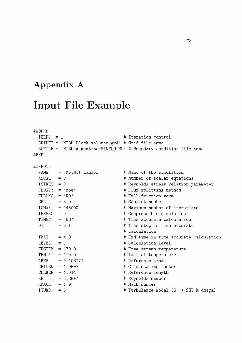
73

Appendix A

Input File Example

&WORKS

IOLD1 = 1 # Iteration control

GRIDFI = ’MIBU-Block-volumes.grd’ # Grid file name

BCFILE = ’MIBU-August-bc-FINFLO.BC’ # Boundary condition file name

&END

&INPUTS

NAME = ’MetNet Lander’ # Name of the simulation

KSCAL = 0 # Number of scalar equations

ISTRES = 0 # Reynolds stress-relation parameter

FLUXTY = ’roe’ # Flux splitting method

FULLNC = ’NO’ # Full friction term

CFL = 3.0 # Courant number

ICMAX = 145000 # Maximum number of iterations

IPRESC = 0 # Compressible simulation

TIMEC = ’NO’ # Time accurate calculation

DT = 0.1 # Time step in time accurate

# calculation

TMAX = 4.0 # End time in time accurate calculation

LEVEL = 1 # Calculation level

FRSTEM = 170.0 # Free stream temperature

TEMINI = 170.0 # Initial temperature

AREF = 0.403771 # Reference area

GRILEN = 1.0E-3 # Grid scaling factor

CHLREF = 1.014 # Reference length

RE = 3.2E+7 # Reynolds number

RMACH = 1.9 # Mach number

ITURB = 6 # Turbulence model (6 -> SST k-omega)

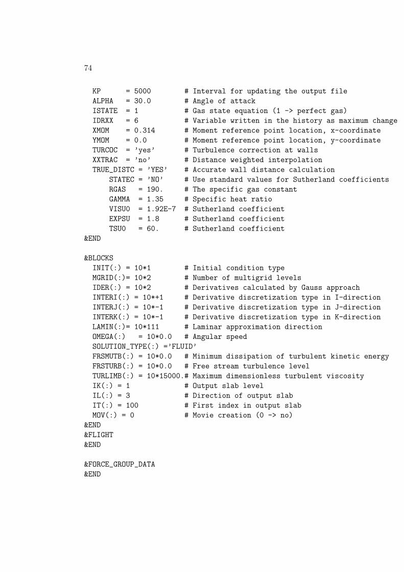
74

KP = 5000 # Interval for updating the output file

ALPHA = 30.0 # Angle of attack

ISTATE = 1 # Gas state equation (1 -> perfect gas)

IDRXX = 6 # Variable written in the history as maximum change

XMOM = 0.314 # Moment reference point location, x-coordinate

YMOM = 0.0 # Moment reference point location, y-coordinate

TURCOC = ’yes’ # Turbulence correction at walls

XXTRAC = ’no’ # Distance weighted interpolation

TRUE_DISTC = ’YES’ # Accurate wall distance calculation

STATEC = ’NO’ # Use standard values for Sutherland coefficients

RGAS = 190. # The specific gas constant

GAMMA = 1.35 # Specific heat ratio

VISU0 = 1.92E-7 # Sutherland coefficient

EXPSU = 1.8 # Sutherland coefficient

TSU0 = 60. # Sutherland coefficient

&END

&BLOCKS

INIT(:) = 10*1 # Initial condition type

MGRID(:)= 10*2 # Number of multigrid levels

IDER(:) = 10*2 # Derivatives calculated by Gauss approach

INTERI(:) = 10*+1 # Derivative discretization type in I-direction

INTERJ(:) = 10*-1 # Derivative discretization type in J-direction

INTERK(:) = 10*-1 # Derivative discretization type in K-direction

LAMIN(:)= 10*111 # Laminar approximation direction

OMEGA(:) = 10*0.0 # Angular speed

SOLUTION_TYPE(:) =’FLUID’

FRSMUTB(:) = 10*0.0 # Minimum dissipation of turbulent kinetic energy

FRSTURB(:) = 10*0.0 # Free stream turbulence level

TURLIMB(:) = 10*15000.# Maximum dimensionless turbulent viscosity

IK(:) = 1 # Output slab level

IL(:) = 3 # Direction of output slab

IT(:) = 100 # First index in output slab

MOV(:) = 0 # Movie creation (0 -> no)

&END

&FLIGHT

&END

&FORCE_GROUP_DATA

&END

75

Appendix B

Aerydynamic coefficients of theMIBD case

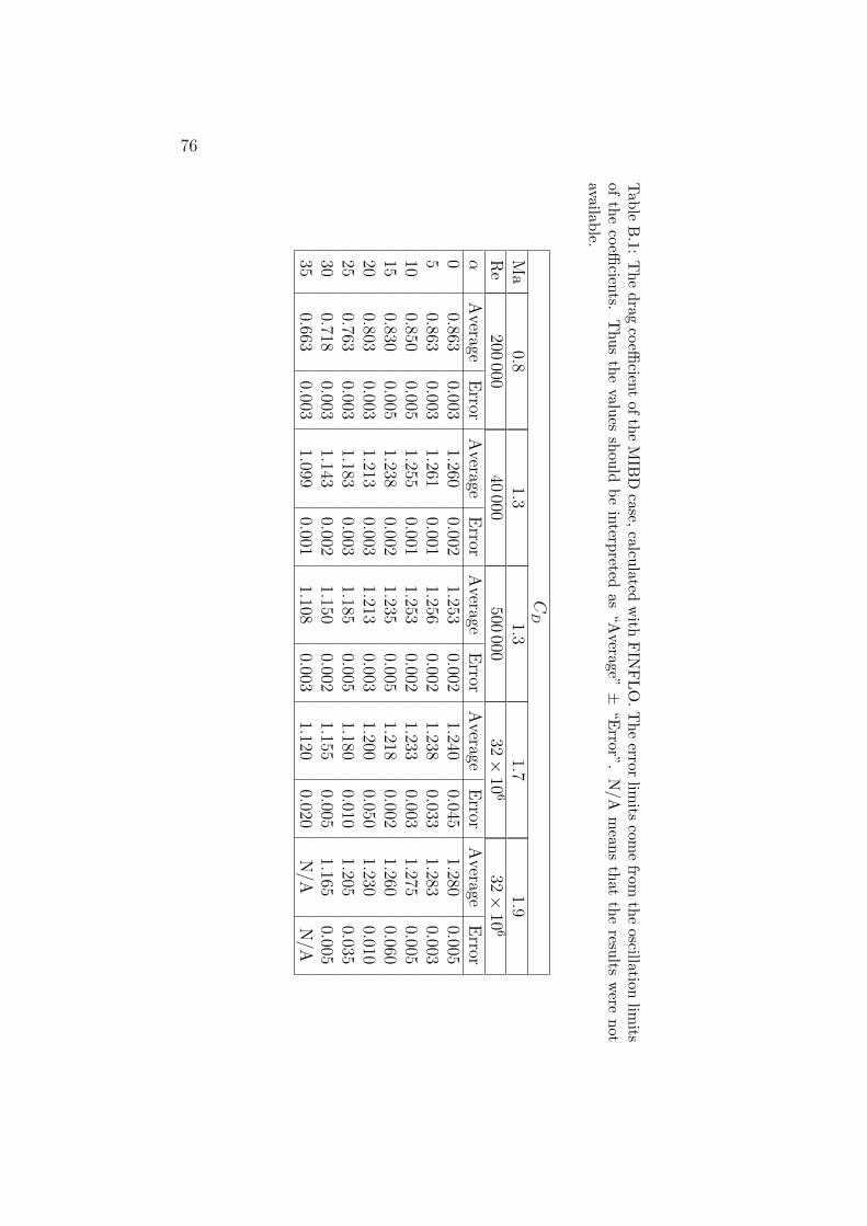
76

Tab

leB

.1:T

he

dra

gco

efficien

tof

the

MIB

Dcase,

calculated

with

FIN

FL

O.

The

errorlim

itscom

efrom

the

oscillationlim

itsof

the

coeffi

cients.

Thu

sth

eva

lues

should

be

interp

retedas

“Average”

±“E

rror”.N

/Am

eans

that

the

results

were

not

availab

le.

CD

Ma

0.81.3

1.31.7

1.9R

e200

00040

000500

00032×

106

32×

106

αA

verageE

rrorA

verageE

rrorA

verageE

rrorA

verageE

rrorA

verageE

rror0

0.8630.003

1.2600.002

1.2530.002

1.2400.045

1.2800.005

50.863

0.0031.261

0.0011.256

0.0021.238

0.0331.283

0.00310

0.8500.005

1.2550.001

1.2530.002

1.2330.003

1.2750.005

150.830

0.0051.238

0.0021.235

0.0051.218

0.0021.260

0.06020

0.8030.003

1.2130.003

1.2130.003

1.2000.050

1.2300.010

250.763

0.0031.183

0.0031.185

0.0051.180

0.0101.205

0.03530

0.7180.003

1.1430.002

1.1500.002

1.1550.005

1.1650.005

350.663

0.0031.099

0.0011.108

0.0031.120

0.020N

/AN

/A

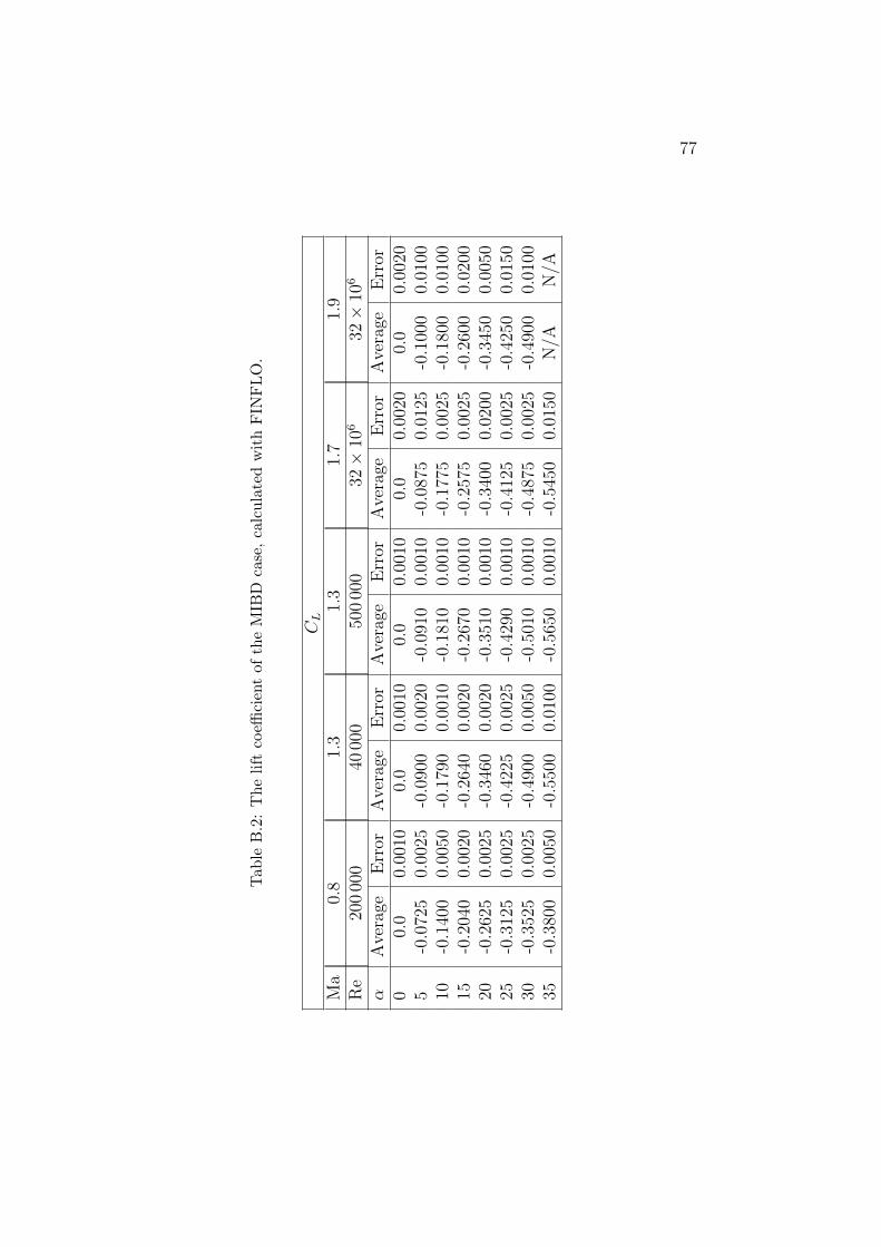
77

Tab

leB

.2:

Th

eli

ftco

effici

ent

ofth

eM

IBD

case

,ca

lcu

late

dw

ith

FIN

FL

O.

CL

Ma

0.8

1.3

1.3

1.7

1.9

Re

200

000

4000

050

000

032×

106

32×

106

αA

vera

geE

rror

Ave

rage

Err

orA

vera

geE

rror

Ave

rage

Err

orA

vera

geE

rror

00.

00.

0010

0.0

0.00

100.

00.

0010

0.0

0.00

200.

00.

0020

5-0

.072

50.

0025

-0.0

900

0.00

20-0

.091

00.

0010

-0.0

875

0.01

25-0

.100

00.

0100

10-0

.140

00.

0050

-0.1

790

0.00

10-0

.181

00.

0010

-0.1

775

0.00

25-0

.180

00.

0100

15-0

.204

00.

0020

-0.2

640

0.00

20-0

.267

00.

0010

-0.2

575

0.00

25-0

.260

00.

0200

20-0

.262

50.

0025

-0.3

460

0.00

20-0

.351

00.

0010

-0.3

400

0.02

00-0

.345

00.

0050

25-0

.312

50.

0025

-0.4

225

0.00

25-0

.429

00.

0010

-0.4

125

0.00

25-0

.425

00.

0150

30-0

.352

50.

0025

-0.4

900

0.00

50-0

.501

00.

0010

-0.4

875

0.00

25-0

.490

00.

0100

35-0

.380

00.

0050

-0.5

500

0.01

00-0

.565

00.

0010

-0.5

450

0.01

50N

/AN

/A

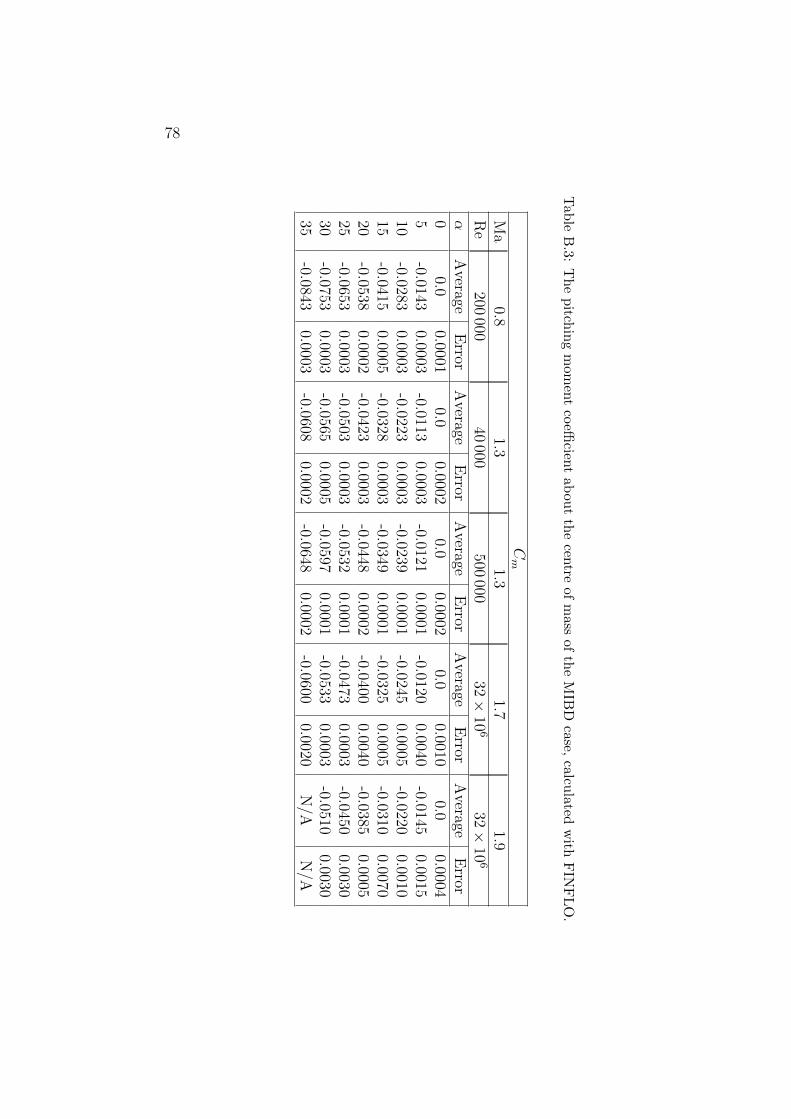
78

Tab

leB

.3:T

he

pitch

ing

mom

ent

coeffi

cient

abou

tth

ecen

treof

mass

ofth

eM

IBD

case,calcu

latedw

ithF

INF

LO

.

Cm

Ma

0.81.3

1.31.7

1.9R

e200

00040

000500

00032×

106

32×

106

αA

verageE

rrorA

verageE

rrorA

verageE

rrorA

verageE

rrorA

verageE

rror0

0.00.0001

0.00.0002

0.00.0002

0.00.0010

0.00.0004

5-0.0143

0.0003-0.0113

0.0003-0.0121

0.0001-0.0120

0.0040-0.0145

0.001510

-0.02830.0003

-0.02230.0003

-0.02390.0001

-0.02450.0005

-0.02200.0010

15-0.0415

0.0005-0.0328

0.0003-0.0349

0.0001-0.0325

0.0005-0.0310

0.007020

-0.05380.0002

-0.04230.0003

-0.04480.0002

-0.04000.0040

-0.03850.0005

25-0.0653

0.0003-0.0503

0.0003-0.0532

0.0001-0.0473

0.0003-0.0450

0.003030

-0.07530.0003

-0.05650.0005

-0.05970.0001

-0.05330.0003

-0.05100.0030

35-0.0843

0.0003-0.0608

0.0002-0.0648

0.0002-0.0600

0.0020N

/AN

/A

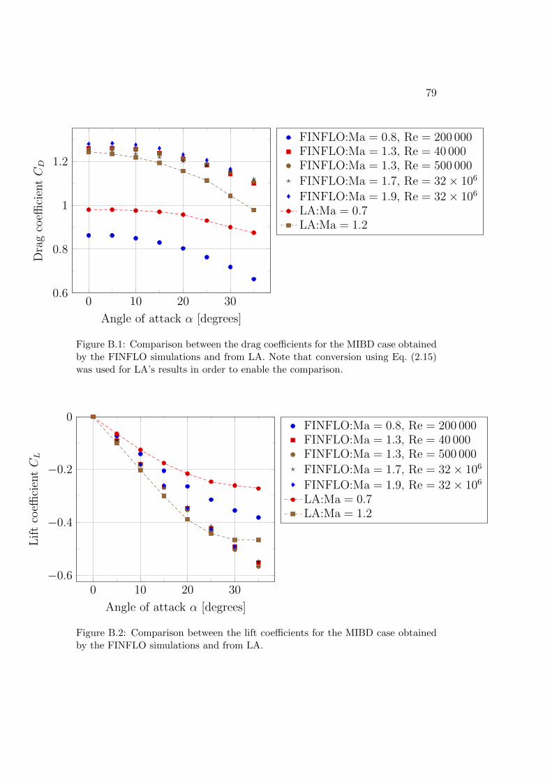
79

0 10 20 300.6

0.8

1

1.2

Angle of attack α [degrees]

Dra

gco

effici

entCD

FINFLO:Ma = 0.8, Re = 200 000FINFLO:Ma = 1.3, Re = 40 000FINFLO:Ma = 1.3, Re = 500 000

FINFLO:Ma = 1.7, Re = 32× 106

FINFLO:Ma = 1.9, Re = 32× 106

LA:Ma = 0.7LA:Ma = 1.2

Figure B.1: Comparison between the drag coefficients for the MIBD case obtainedby the FINFLO simulations and from LA. Note that conversion using Eq. (2.15)was used for LA’s results in order to enable the comparison.

0 10 20 30−0.6

−0.4

−0.2

0

Angle of attack α [degrees]

Lif

tco

effici

entCL

FINFLO:Ma = 0.8, Re = 200 000FINFLO:Ma = 1.3, Re = 40 000FINFLO:Ma = 1.3, Re = 500 000

FINFLO:Ma = 1.7, Re = 32× 106

FINFLO:Ma = 1.9, Re = 32× 106

LA:Ma = 0.7LA:Ma = 1.2

Figure B.2: Comparison between the lift coefficients for the MIBD case obtainedby the FINFLO simulations and from LA.

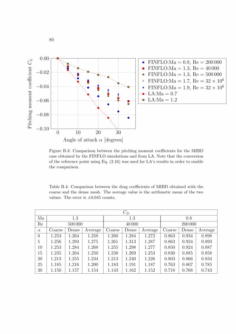
80

0 10 20 30−0.10

−0.08

−0.06

−0.04

−0.02

0.00

Angle of attack α [degrees]

Pit

chin

gm

omen

tco

effici

entCL FINFLO:Ma = 0.8, Re = 200 000

FINFLO:Ma = 1.3, Re = 40 000FINFLO:Ma = 1.3, Re = 500 000

FINFLO:Ma = 1.7, Re = 32× 106

FINFLO:Ma = 1.9, Re = 32× 106

LA:Ma = 0.7LA:Ma = 1.2

Figure B.3: Comparison between the pitching moment coefficients for the MIBDcase obtained by the FINFLO simulations and from LA. Note that the conversionof the reference point using Eq. (2.16) was used for LA’s results in order to enablethe comparison.

Table B.4: Comparison between the drag coefficients of MIBD obtained with thecoarse and the dense mesh. The average value is the arithmetic mean of the twovalues. The error is ±0.045 counts.

CDMa 1.3 1.3 0.8Re 500 000 40 000 200 000α Coarse Dense Average Coarse Dense Average Coarse Dense Average0 1.253 1.264 1.258 1.260 1.284 1.272 0.863 0.934 0.8985 1.256 1.294 1.275 1.261 1.313 1.287 0.863 0.924 0.89310 1.253 1.284 1.268 1.255 1.298 1.277 0.850 0.924 0.88715 1.235 1.264 1.250 1.238 1.269 1.253 0.830 0.885 0.85820 1.213 1.255 1.234 1.213 1.240 1.226 0.803 0.866 0.83425 1.185 1.216 1.200 1.183 1.191 1.187 0.763 0.807 0.78530 1.150 1.157 1.154 1.143 1.162 1.152 0.718 0.768 0.743

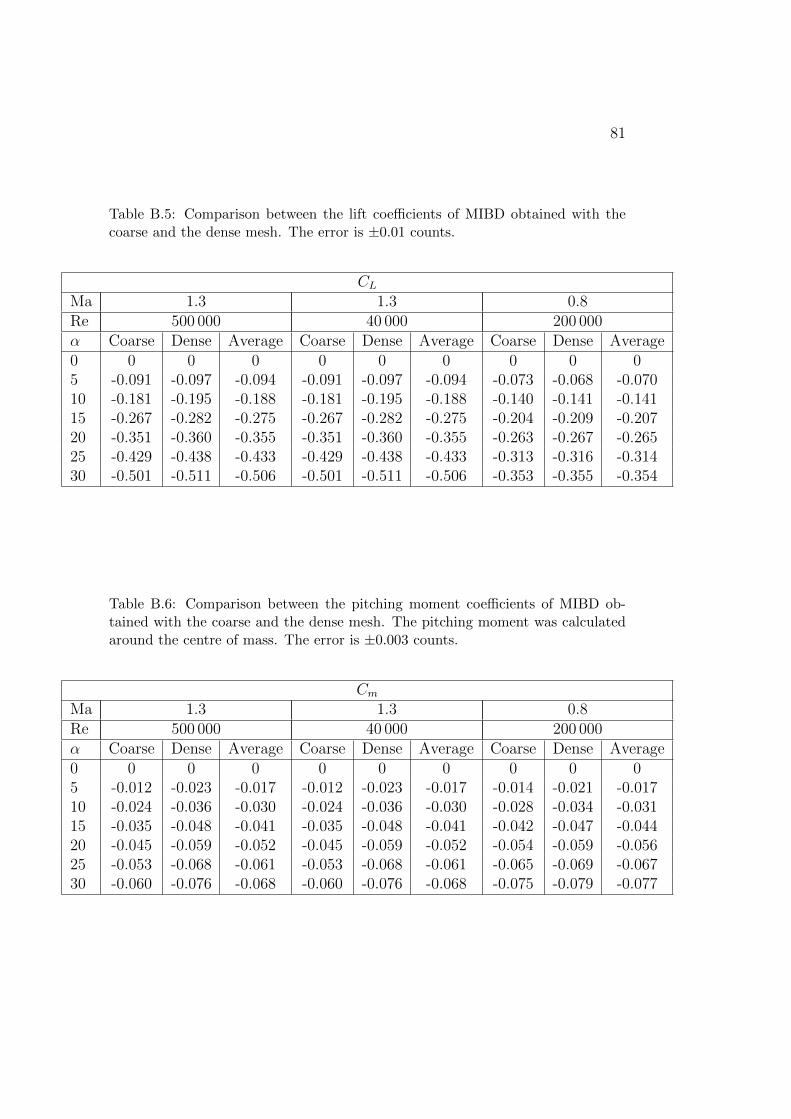
81

Table B.5: Comparison between the lift coefficients of MIBD obtained with thecoarse and the dense mesh. The error is ±0.01 counts.

CLMa 1.3 1.3 0.8Re 500 000 40 000 200 000α Coarse Dense Average Coarse Dense Average Coarse Dense Average0 0 0 0 0 0 0 0 0 05 -0.091 -0.097 -0.094 -0.091 -0.097 -0.094 -0.073 -0.068 -0.07010 -0.181 -0.195 -0.188 -0.181 -0.195 -0.188 -0.140 -0.141 -0.14115 -0.267 -0.282 -0.275 -0.267 -0.282 -0.275 -0.204 -0.209 -0.20720 -0.351 -0.360 -0.355 -0.351 -0.360 -0.355 -0.263 -0.267 -0.26525 -0.429 -0.438 -0.433 -0.429 -0.438 -0.433 -0.313 -0.316 -0.31430 -0.501 -0.511 -0.506 -0.501 -0.511 -0.506 -0.353 -0.355 -0.354

Table B.6: Comparison between the pitching moment coefficients of MIBD ob-tained with the coarse and the dense mesh. The pitching moment was calculatedaround the centre of mass. The error is ±0.003 counts.

CmMa 1.3 1.3 0.8Re 500 000 40 000 200 000α Coarse Dense Average Coarse Dense Average Coarse Dense Average0 0 0 0 0 0 0 0 0 05 -0.012 -0.023 -0.017 -0.012 -0.023 -0.017 -0.014 -0.021 -0.01710 -0.024 -0.036 -0.030 -0.024 -0.036 -0.030 -0.028 -0.034 -0.03115 -0.035 -0.048 -0.041 -0.035 -0.048 -0.041 -0.042 -0.047 -0.04420 -0.045 -0.059 -0.052 -0.045 -0.059 -0.052 -0.054 -0.059 -0.05625 -0.053 -0.068 -0.061 -0.053 -0.068 -0.061 -0.065 -0.069 -0.06730 -0.060 -0.076 -0.068 -0.060 -0.076 -0.068 -0.075 -0.079 -0.077

82

83

Appendix C

Aerodynamic coefficients of theAIBD case

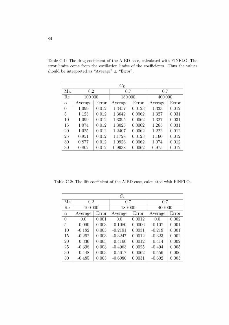
84

Table C.1: The drag coefficient of the AIBD case, calculated with FINFLO. Theerror limits come from the oscillation limits of the coefficients. Thus the valuesshould be interpreted as “Average” ± “Error”.

CDMa 0.2 0.7 0.7Re 100 000 180 000 400 000α Average Error Average Error Average Error0 1.099 0.012 1.3457 0.0123 1.333 0.0125 1.123 0.012 1.3642 0.0062 1.327 0.03110 1.099 0.012 1.3395 0.0062 1.327 0.03115 1.074 0.012 1.3025 0.0062 1.265 0.03120 1.025 0.012 1.2407 0.0062 1.222 0.01225 0.951 0.012 1.1728 0.0123 1.160 0.01230 0.877 0.012 1.0926 0.0062 1.074 0.01230 0.802 0.012 0.9938 0.0062 0.975 0.012

Table C.2: The lift coefficient of the AIBD case, calculated with FINFLO.

CLMa 0.2 0.7 0.7Re 100 000 180 000 400 000α Average Error Average Error Average Error0 0.0 0.001 0.0 0.0012 0.0 0.0025 -0.090 0.003 -0.1080 0.0006 -0.107 0.00110 -0.182 0.003 -0.2191 0.0031 -0.219 0.00115 -0.262 0.003 -0.3247 0.0012 -0.323 0.00220 -0.336 0.003 -0.4160 0.0012 -0.414 0.00225 -0.398 0.003 -0.4963 0.0025 -0.494 0.00530 -0.448 0.003 -0.5617 0.0062 -0.556 0.00630 -0.485 0.003 -0.6080 0.0031 -0.602 0.003

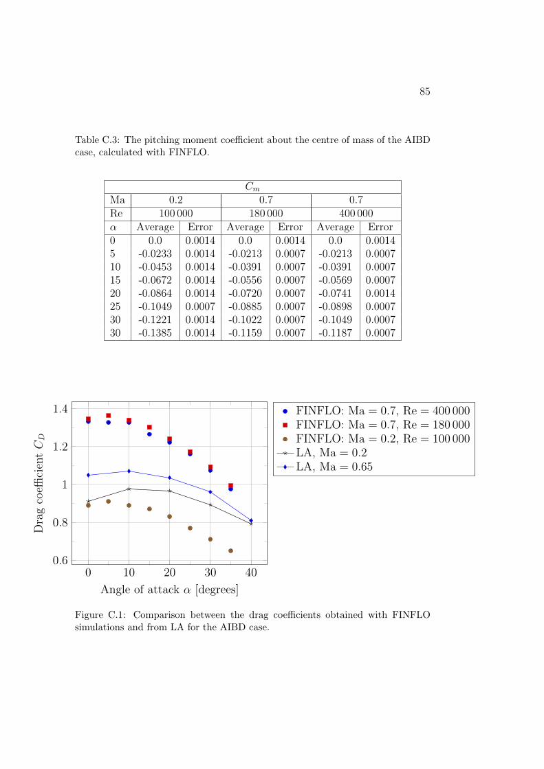
85

Table C.3: The pitching moment coefficient about the centre of mass of the AIBDcase, calculated with FINFLO.

CmMa 0.2 0.7 0.7Re 100 000 180 000 400 000α Average Error Average Error Average Error0 0.0 0.0014 0.0 0.0014 0.0 0.00145 -0.0233 0.0014 -0.0213 0.0007 -0.0213 0.000710 -0.0453 0.0014 -0.0391 0.0007 -0.0391 0.000715 -0.0672 0.0014 -0.0556 0.0007 -0.0569 0.000720 -0.0864 0.0014 -0.0720 0.0007 -0.0741 0.001425 -0.1049 0.0007 -0.0885 0.0007 -0.0898 0.000730 -0.1221 0.0014 -0.1022 0.0007 -0.1049 0.000730 -0.1385 0.0014 -0.1159 0.0007 -0.1187 0.0007

0 10 20 30 400.6

0.8

1

1.2

1.4

Angle of attack α [degrees]

Dra

gco

effici

entCD

FINFLO: Ma = 0.7, Re = 400 000FINFLO: Ma = 0.7, Re = 180 000FINFLO: Ma = 0.2, Re = 100 000LA, Ma = 0.2LA, Ma = 0.65

Figure C.1: Comparison between the drag coefficients obtained with FINFLOsimulations and from LA for the AIBD case.

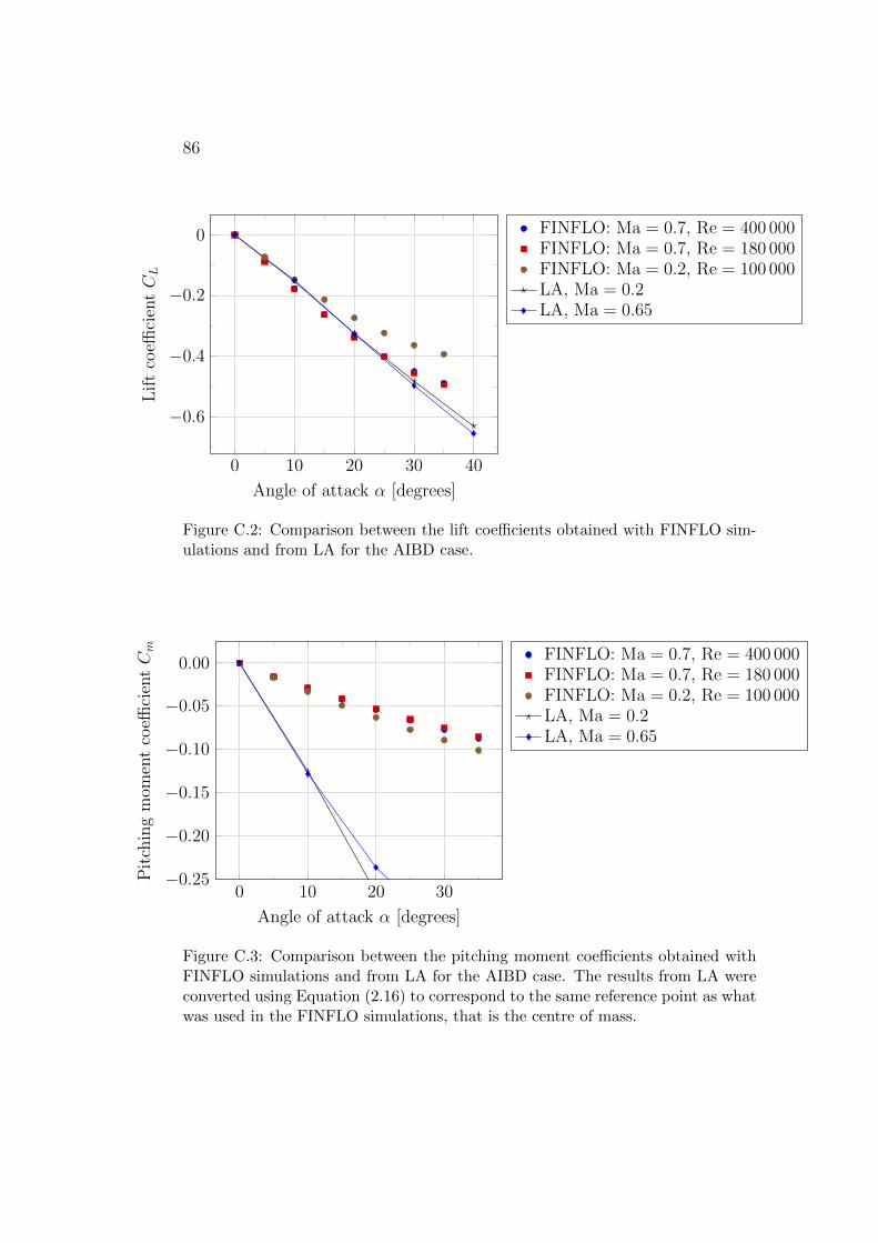
86

0 10 20 30 40

−0.6

−0.4

−0.2

0

Angle of attack α [degrees]

Lif

tco

effici

entCL

FINFLO: Ma = 0.7, Re = 400 000FINFLO: Ma = 0.7, Re = 180 000FINFLO: Ma = 0.2, Re = 100 000LA, Ma = 0.2LA, Ma = 0.65

Figure C.2: Comparison between the lift coefficients obtained with FINFLO sim-ulations and from LA for the AIBD case.

0 10 20 30−0.25

−0.20

−0.15

−0.10

−0.05

0.00

Angle of attack α [degrees]

Pit

chin

gm

omen

tco

effici

entCm FINFLO: Ma = 0.7, Re = 400 000

FINFLO: Ma = 0.7, Re = 180 000FINFLO: Ma = 0.2, Re = 100 000LA, Ma = 0.2LA, Ma = 0.65

Figure C.3: Comparison between the pitching moment coefficients obtained withFINFLO simulations and from LA for the AIBD case. The results from LA wereconverted using Equation (2.16) to correspond to the same reference point as whatwas used in the FINFLO simulations, that is the centre of mass.