Proc IMechE Part O: J Risk and Reliability Fault tree ...nusbaumer.tripod.com/...FaultTreeLinkingVersusEventTreeLinking.pdf · Fault tree linking versus event tree linking approaches:

Special Issue Article

Proc IMechE Part O:J Risk and Reliability227(3) 315–326� IMechE 2013Reprints and permissions:sagepub.co.uk/journalsPermissions.navDOI: 10.1177/1748006X13490260pio.sagepub.com

Fault tree linking versus event treelinking approaches: a reasonedcomparison

Olivier Nusbaumer1 and Antoine Rauzy2

AbstractTwo well-known modelling approaches are in use in probabilistic risk assessment: fault tree linking and event tree linking.The question of which modelling approach is most appropriate for specific applications has been extensively, if not emo-tionally, debated among experts in the past two decades, addressing both modelling and quantification issues. In this arti-cle, we determine their degree of equivalence and build ‘methodological bridges’ between the two approaches from amathematical and algorithmic perspective. We show that, under certain conditions, both modelling approaches areequivalent. Since both fault tree linking and event tree linking approaches are subject to limitations and approximations,established bridges make it possible to formulate important recommendations for probabilistic risk assessment practi-tioners and quantification engine developers.

KeywordsProbabilistic risk assessment, methodology, modelling, quantification engines

Date received: 20 September 2012; accepted: 26 April 2013

Introduction

Two well-known modelling methodologies are in use inprobabilistic safety assessment (PSA) and probabilisticrisk assessment (PRA), see for example, Kumamotoand Henley1 for an introduction: fault tree linking(FTL) and event tree linking (ETL). These twoapproaches are described and compared almost fromthe beginning of Nuclear PSA (see e.g. NUREG/CR-23002). The question of which modelling methodologyis most appropriate for specific applications has beenextensively, if not emotionally, debated among expertsin the past three decades, addressing both modellingand quantification issues. The already cited NUREG/CR-2300 (section 6.3) remarked that ‘Overall, the basicconceptual difference between the methods is where theprocess quantification (conversion to from symbolic rep-resentation to numerical results takes places)’.

This article aims to give a solid ground and to com-plement this assertion by comparing the twoapproaches from a mathematical and algorithmic per-spective. As a starting point, we assume that bothapproaches start with the same virtual model. The FTLapproach quantification algorithms work on that vir-tual model, or on a model that is close to that virtualmodel. On the contrary, the ETL approach first

develops the virtual model so to make event treesequences pair wisely disjoint. This development is sup-posed to preserve logical equivalence. In practice how-ever, the two approaches give different results, becausedifferent modelling and algorithmic strategies areapplied.

This situation is however not as bad as it may seemat first glance: it is actually possible to build ‘methodo-logical bridges’ between the two approaches and toestablish formally their degree of equivalence. A gen-eral assumption in sciences is that two objects understudy can be considered as equivalent if they cannot bedistinguished with the observation means at hand. Inour case, objects are models and observation means arequantification algorithms.

Quantification algorithms can be classified into twocategories: those computing a sum of disjoint productsand those computing a set of minimal cutsets. The for-mers evaluate states, i.e. valuations of basic events to

1Leibstadt Nuclear Power Plant, Leibstadt, Switzerland2Ecole Polytechnique, Palaiseau, France

Corresponding author:

Antoine Rauzy, Ecole Polytechnique, Palaiseau 91128, France.

Email: [email protected]

either true or false, while the latter perform a coherent/monotone approximation of the models. In both cases,cutoffs can be applied. Quantification algorithms ofRiskSprectrum3,4 and CAFTA5,6 are based on minimalcutsets calculation. The ETL approach can be seen asthe partial application of a sum of disjoint productsalgorithm. Bryant’s binary decision diagrams7 adaptedfor PSA/PRA quantification (see e.g. Rauzy8 for a sur-vey) also belong to this category. With respect to thisclassification, we can define two natural equivalencerelations on PSA/PRA models.

� Strong equivalence: two models are strongly equiva-lent if they agree on global states (minterms) whoseprobability (evaluated in a certain way) is bigger thanthe given cutoff, i.e. if they cannot be distinguishedby means of a sum of disjoint products algorithm.

� Weak equivalence: two models are weakly equiva-lent if they agree on minimal cutsets whose prob-ability is bigger than the given cutoff, i.e. if theycannot be distinguished by means of a minimal cut-sets algorithm.

Weak equivalence is indeed coarser than strong equiva-lence or, to put it into another way, sum of disjointproducts algorithms give finer results than minimal cut-sets algorithms. This precision comes with a severeincrease of necessary computing resources.

Strong and weak equivalence give a firm mathemati-cal ground to compare FTL and ETL approaches.Basically, we show that the two approaches are weaklyequivalent and that the approximations are in generalaccurate on coherent models. These results clarifyEpstein and Rauzy’s statements about PSA/PRAquantification.9

Since problems in quantification can arise mainly onnon-coherent models, it is of interest to study carefullywhere non-coherence comes from. We discuss here thisissue based on responses to a questionnaire provided bya large international panel of PSA/PRA analysts.

The remainder of the article is organized as follows.First we introduce the mathematical and algorithmicframework of PSA/PRA. Then, we present both FTLand ETL approaches by means of a small example. Weestablish formally their degree of equivalence, first forcoherent models, then for non-coherent ones. Finally,we discuss where non-coherence comes from.

Mathematical preliminaries

In this section, we review the basics about Booleanlogic involved in fault tree and event tree analysis. Fora more thorough treatment of the subject, the reader isreferred to Rauzy.10

Throughout this article we consider fault tree andevent tree models. Fault trees and event trees are inter-preted as Boolean formulas built over a finite set of vari-ables, so-called basic events, and logical connectives ‘+’

(or), ‘�’ (and) and ‘2’ (not). Other connectives, such ask-out-of-n and others can be easily derived from those.

A ‘literal’ is either a basic event or its negation. A‘product’ is a conjunction of literals that does not con-tain both a basic event and its negation. A product ispositive if it contains no negated basic event. A ‘sum ofproducts’ is a set of products interpreted as their dis-junction. Two products are disjoint if there is at leastone basic event occurring positively in one of them andnegatively in the other. A ‘sum of disjoint products’(SDP) is a sum of products whose products are pairwisely disjoint. A ‘minterm’, relative to a set of basicevents, is a product that contains a literal for each basicevent in the set. By construction, two different min-terms are disjoint. Minterms one-to-one correspondwith truth assignments of basic events. For that reason,the following property holds.

Property 1

Any Boolean formula is equivalent to a unique sum ofminterms.

Consider for instance the Boolean formula F = A�B+2A�C. The formula F can be expanded into a sumof minterms, relatively to the set of basic events {A, B,C}, as follows.

Minterms(F)= A � B � C+A � B� C+

� A � B � C+� A� B � C

We shall say that a minterm p belongs to a formula F,and shall denote p2 F, if p occurs in Minterms(F).Similarly, we shall write F 4 G, when Minterms(F) 4Minterms(G) and F[G when Minterms(F) =Minterms(G), i.e. when F and G are logically equivalent.Note that logical equivalence is the strongest equivalencerelation over models. Two logically equivalent models areindistinguishable by any correct quantification algorithm.

Let p and r be two minterms. We say that p 4 r, ifany basic event that occurs positively in p occurs posi-tively in r as well. For instance, we have A�B�2C4A�B�C.

A Boolean formula F is coherent if for any two min-terms p and r such that p2F and p 4 r, then r2F. Itis easy to verify that any formula built only over basicevents and connectives ‘+’ and ‘.’ is coherent.

Let p be a positive product. We denote by p’ theminterm built by completing p with the negative literalsbuilt over basic events that do not show up in p. Forinstance, in the above example, we have

(A � B)9=A � B � �C and C9=� A ��B � C

A cutset of a Boolean formula F is defined as a positiveproduct p, such that p’2 F. A cutset p is minimal ifno subproduct of p is a cutset of F. Consider again theabove example, the formula F admits the following cut-set and minimal cutsets (MCS)

Cutsets(F)= fA � B, C, A � B � Cg, MCS(F)= fA � B, Cg

316 Proc IMechE Part O: J Risk and Reliability 227(3)

MCS(F) can be interpreted as a sum of products, i.e. aBoolean formula. As illustrated by the above example,F and MCS(F) may differ.

Model quantification

In PRAmodels, because of basic events that are repeatedhere and there, there is no efficient way to quantify thereliability indicators of interest, such as the top-eventprobability and importance factors. From a theoreticalviewpoint, this impossibility has been formally estab-lished by Valiant.11 Therefore, all of the algorithmsknown so far have two important characteristics.

1. Either they compute an approximation of the indi-cator of interest or they are subject to the exponen-tial blow-up of computation resources, and most ofthe time they suffer from both drawbacks.

2. They compute an intermediate form of the modelfrom which the reliability indicators can becalculated.

From a practical viewpoint, there are so far only twocategories of algorithms.

1. Algorithms that compute minimal cutsets of themodel and perform quantifications from these min-imal cutsets. These algorithms are used mostly bythe FTL approach.

2. Algorithms that compute a SDP and performquantifications of this SDP. These algorithms areused mostly by the ETL approach.

Minimal cutsets algorithms

The first category is historically the first to have beendeveloped and the most widely used. The algorithmimplemented in RiskSprectrum,4 which is derived fromMOCUS3 and the one implemented in CAFTA compu-tation engine5,6 belong to this category. The fact thatCAFTA computation engine uses Minato’s ZBDD12 toencode MCS changes nothing to the matter: all quantifi-cations are performed through (an encoding of) MCS.MOCUS, like algorithms, compute MCS top-down.ZBDD-based algorithms compute MCS bottom-up.Note that an important step forward has been maderecently by Rauzy who proposed a branch and deducealgorithmic scheme to compute MCS.13 This workmakes it possible to implement very efficient MCS calcu-lation engines and to better understand the algorithmicissues at stake.

The following property holds that characterizes therelationship between a formula and its minimal cutsets.

Property 2

Let F be a Boolean Formula. Then, F 4 MCS(F).Moreover, MCS(F) is the smallest monotone formulacontaining F.

As a consequence, F = MCS(F) if, and only if, F iscoherent.

This property has been stated and proved inRauzy.10 Property 2 ensures that by computing mini-mal cutsets, we make no logical approximation if themodel under study is coherent and a conservativeapproximation if it is non-coherent. By conservative wemean here that the sum of minimal cutsets encode allfailure states (minterms) of the original model, pluspossibly some that are not in the original model.

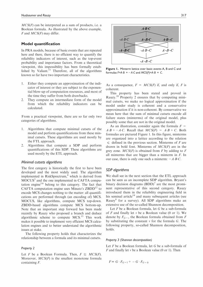
As an illustration, consider again the formula F =A�B+2A�C. Recall that MCS(F) = A�B+C. Bothformulas are pictured Figure 1. In this figure, mintermsare organized into a lattice according to the relation4 defined in the previous section. Minterms of F aredrawn in bold font. Minterms of MCS(F) are in thegrey zone. MCS(F) is obtained from F by adding to Fall minterms that are bigger than a minterm in F. Inour case, there is only one such a minterm: 2A�B�C.

SDP algorithms

We shall see in the next section that the ETL approachcan be seen as an incomplete SDP algorithm. Bryant’sbinary decision diagrams (BDD)7 are the most promi-nent representative of this second category. Rauzyintroduced them in the reliability engineering field inhis seminal article14 and many subsequent articles (seeRauzy8 for a survey). All SDP algorithms make anextensive use of the so-called Shannon decomposition.

Let F be a Boolean formula, let G be a sub-formulaof F and finally let v be a Boolean value (0 or 1). Wedenote by FG=v the Boolean formula obtained from Fby substituting the constant v for the formula G. Thefollowing property, so-called Shannon decomposition,holds.

Property 3 (Shannon decomposition)

Let F be a Boolean formula, let G be a sub-formula ofF and finally let v be a Boolean value (0 or 1). Then

F[ G � FG=1+� G � FG=0

Figure 1. Minterm lattice over basic events A, B and C andformulas F=A�B + 2A�C and MCS(F)=A�B + C.

Nusbaumer and Rauzy 317

G is called the pivot of the decomposition. In the caseof BDD, pivots are always basic events. In the case ofETL development, it can be an intermediate event aswell.

Consider for instance the formula F = A�B + A�C+ B�C, i.e. a 2-out-of-3 over basic events A, B and C.This sum of products can be rewritten into a logicallyequivalent SDP by successive applications of theShannon decomposition

F= A �B+A �C+B �C[A �FA=1 +�A �FA=0=A � (1 �B+1 �C+B �C)+�A � (0 �B+0 �C+B �C)=A(B+C+ B �C)+�A �B �C

A � (B(B+C+BC)B=1 +�B � (B+C+B �C)B=0

+�A �B �C=A � (B+�B �C) +�A �B �C=A �B+ A�B �C + �A �B �C

In the sequel we shall denote by SDP(F) the SDPobtained from F by some SDP algorithm. Indeed,SDP(F) is by no means unique. But since the Shannondecomposition preserves the logical equivalence,SDP(F)[ F for any correct algorithm.

Probability calculation

Let F be a Boolean formula. We say that F has a prob-ability structure if it comes with a function p(.) thatassociates a probability with each basic event of F. Byextension, we denote by p(F) the probability of the for-mula F. The well-known Sylvester-Poincare develop-ment, also called inclusion-exclusion principle, makes itpossible to compute the probability of a sum of prod-ucts from the probabilities of basic events.

Property 4 (Sylvester-Poincare development)

Let F =P

i=1,.,npi be a sum of products. Then, thefollowing equality holds

p(F)=S14 i4 np(pi) � S14 i1 4 i2 4 np(pi1pi2 )

+ . . . +� 1pS14 i1 4 ...:4 ip 4 np(pi1 . . . pip )

+ . . . +� 1np(p1 . . . pn)

We say that a model is solved exactly (but not obligato-rily completely) when the full Sylvester-Poincare devel-opment is applied. Unfortunately, applying thisdevelopment fully is exponential in the number ofproducts. For this reason, most (FTL) quantificationengines approximate it by computing only the first termof this development (rare event approximation). This isa problem if individual probabilities are large or if themodel is not coherent. Otherwise, the rare eventapproximation is, in general, quite accurate.

Another approximation, the so-called ‘min cut upperbound’ (MCUB), which is also first order and is oftenused in practice, gives better approximations than the

rare event approximation. The MCUB formula is asfollows

p(F) ffi 1�Y

i

1� p(pi)ð Þ

As compared with the rare event approximation, theMCUB prevents the top event probability exceed 1. Onthe other hand, as a first-order technique, it cannot giveexact results in most cases (if the formula is coherent, italways gives conservative results though).

In the case where the formula is a SDP, the rareevent approximation gives even the exact probability,for all subsequent terms are cancelled (because theyinvolved at least two products and products are pairwisely disjoint). The following property holds.

Property 5

Let F =P

i=1,.,npi be a sum of products. The follow-ing inequality holds

p(F)4Si=1, ..., np(pi)

Moreover, if for each basic event E, p(E)� 1, then theapproximation is accurate

p(F)’ Si=1, ..., np(pi)

If F is a SDP, then the inequality becomes equality

p(F) =Si=1, ..., np(pi)

Let us summarize what we have obtained so far. Let Fbe a coherent Boolean formula. Then, to get the exactprobability of F we can do any of the followingoperations.

� Build SDP(F), then calculate the first term of theSylvester-Poincare development on SDP(F).

� Build MCS(F), then calculate the full Sylvester-Poincare development on MCS(F).

� Build MCS(F), then SDP(MCS(F)), then calculatethe first term of the Sylvester-Poincare developmenton SDP(MCS(F)).

To get a conservative, and in many practical cases accu-rate, approximation of the probability of F, we can dothe following operations.

� Build MCS(F) then calculate the first term of theSylvester-Poincare development on MCS(F).

As already said, calculating the full Sylvester-Poincaredevelopment (to get an exact probability) is of expo-nential complexity in the number of minimal cutsets.So, calculating a SDP should (and actually is) costly aswell. To illustrate this phenomenon, consider the fol-lowing parametric formula (sum of minimal cutsets)and its transformation into a SDP

Fn =A1 � B1 + . . . +An � Bn


[(A1 � B1 + . . . +An�1 � Bn�1)� An � Bn

+ (A1 � B1s + . . . + An�1 � Bn�1) � �Bn +An � Bn

[Fn�1 � �An � Bn +Fn�1 � �Bn + An � Bn

It follows that SDP(Fn) is more than twice as big asSDP(Fn21) so that the size of SDP(Fn) is exponential inthe number of MCS. Of course, SDP(Fn) can beencoded with a linear size BDD, but there are simpleformulas with a polynomial number of MCS, whichadmit no polynomial size BDD representation (see e.g.Nikolskaia and Nikolskaia15).

If F is non-coherent, we can get a conservativeapproximation of the probability of F by means of anyof the above sequences of operations. Whether thisapproximation is accurate depends on F. For some F,it is quite good, for some others it is awfully bad.Consider for instance, the formula F = 2E, where E isa basic event such that p(E) ’1. In that case, p(F) =12p(E) ’0, while p(MCS(F)) = p(1) = 1.

Cutoffs

Most of the real-life models have a huge number ofminimal cutsets (and even more disjoint products). Somany that it is definitely impossible to encode all ofthem, even using symbolic techniques such as ZBDD.Therefore, cutoffs have to be applied to keep only themost probable minimal cutsets: all MCS whose prob-ability is below a given threshold are discarded. Thisapproximation is indeed not conservative, for it‘ignores’ some of the failure situations.

Let F be a Boolean formula with a probability struc-ture. We denote by MCS5x(F) denote the sum of mini-mal cutsets of F whose probability is bigger than thecutoff value x. Formally

MCS5x(F)= fp inMCS(F); p(p)5xg

The question whether p(MCS5x(F)) is an accurateapproximation is of p(MCS(F)), or in other wordswhether this approximation can be controlled, is some-times not very well understood. The following factsmay clarify the situation.

� It is, in general, possible to tune MCS algorithmsso that they give, while computing MCS5x(F), anupper bound of their error, i.e. of the quantityp(MCS(F)) 2 p(MCS5x(F)), but.

� It is not possible, in general, to estimate this errorwithout running the algorithm. Therefore, the cal-culation of the upper bound on the error is an aposteriori verification.

To understand where the problem comes from, it sufficesto consider a formula F with say a million of minimal cut-sets whose probability is just below the cutoff value. Inthis case, p(MCS5x(F))=0 while p(MCS(F)) ’x3106.One may argue that such a case has little chance to occurin practice. This is partly true, at least for what concerns

the evaluation of the probability of the formula. Based onexperiences they made on a Japanese PSA, Epstein andRauzy9 showed that calculations of so-called importancefactors (indicators that aim to rank basic events accordingto their contribution of the overall risk) can be stronglyimpacted by this phenomenon. Their results have beenconfirmed by Duflot et al.16 on the reference French PSA.

Cutoffs can be also applied by SDP algorithms. Thisapplication is however trickier than for the minimalcutsets case. A first idea would be, given a SDP F anda cutoff value x to discard all of the products of Fwhose probability is lower than x. The problem withthis approach is that it is sensitive to the way the for-mula is written. As an illustration, consider the formulaF = E1+ E2+.+ E1000, where the Ei’s are basicevents. There are different ways to rewrite F as SDP.For instance

F[G=E1 +�E1 � E2 +�E1 � �E2 � E3

+ . . .+� E1 � �E2 � . . .�E999 E1000

F[H =E1 � �E2 � . . .�E999 � �E1000+ E2 � �E3 � . . .

� E999 � �E1000+ . . . +E1000

Assume that the probabilities of the Ei’s are close to1024. Then the probability of the terms2E1�2E2�.2E999 and 2E2�.2E999�2E1000 are closeto (121024)1000’ 1-100031024 = 0.9. Now, if we setup the x a bit below 1024, which is reasonable to keepall of the MCS of F, we will discard the last terms of Gand the first terms of H, resulting into two differentapproximated models and two different approximatedset of MCS. This phenomenon could be a problem inthe ETL approach if one would develop the model tosuch a level of detail that too many cutsets would fallunder the cutoff level. Our experience is that it is defi-nitely a problem on a large PSA model with the BDDtechnology. As a consequence, and it is all whatRauzy’s seminal article10 is about, the truncation shouldconcern only the positive part of disjoint products (thisis what typical MCS engines do).

Let F be a Boolean formula with a probability struc-ture and x be a cutoff value. We denote by SDP5x(F)the SDP obtained from SDP(F) by discarding productswhose probability of the positive part is smaller than x.More formally, let p be a product. We denote by |p|the sub-product of made of positive literals of p. Thenwe define SDP5x(F) as follows

SDP5x(F) = fp 2 SDP(F); p( pj j5xg

Again, SDP5x(F) is not unique because SDP(F) is not.It is worth noting that SDP5x(F) has little chance to be

coherent, even if F and therefore SDP(F) are. As an illus-tration, consider the formula F = A�B + C. Let p(A) =p(B)=p(C)= 1023. Assume that SDP(F) is as followsSDP(F) = A�B�C + A�B�-C +2A�CFinally, let x=1027. We have

SDP5x(F)=A � B� C+� A � C


Clearly, SDP5x(F) is not coherent for the biggest min-term A�B�C has been discarded and there is no way toreintroduce it from the remaining products.

This makes a big difference between MCS5x(F) andSDP5x(F). MCS5x(F) is always coherent. The applica-tion of a cutoff just discards some of the minimal cutsets.The application of cutoffs to SDP gives much less intui-tive results. Conversely to the former, it is a calculationartifact. Nevertheless, the following property holds.

Property 6

Let F be a Boolean formula with a probability structureand let x be a cutoff value. Then the following logicalinequalities hold.

SDP��(F) �MCS��(F)�MCS(SDP��(F))

This property is again a consequence of results pre-sented in Rauzy.10

Wrap-up

Let us summarize the practical consequences ofProperty 1 to Property 6. Let F be a Boolean formulawith a probability structure and let x be a cutoff value.

If F is coherent, then:

� The calculation of MCS(F) preserves the logicalequivalence with F.

� The calculation of MCS5x(F) underestimates F(for it discards failure scenarios): p(MCS5x

(F))4 p(F). The lower the threshold, the better theapproximation.

� The application of the rare-event approximationoverestimates p(MCSx(F)): rare-events(MCSx

(F))5p(MCS5x(F)). The lower the probabilities ofbasic events, the better the approximation.

� The calculation of SDP(F) preserves the logicalequivalence with F.

� The calculation of SDP5x(F) underestimates F:p(SDP5x(F))4 p(F). The lower the threshold, thebetter the approximation.

� The calculation of SDP5x(F) is more optimisticthan the calculation of MCS5x(F)

p(SDP5x(F)) 4 p(MCS5x(F)) 4 rare-events(MCSx(F)).

� MCS5x(F) and SDP5x(F) agree on minimal failurescenarios: MCS5x(F) [MCS(SDP5x(F)).

In some sense, the rare events approximation ‘compen-sates’ the application of a cutoff on minimal cutsets,but indeed one cannot rely on this fact, especially whenprobabilities of basic events are high.

If F is non-coherent, then:

� The calculation of MCS(F) overestimates F:p(MCS(F))5p(F). It may be the case that thisapproximation gives meaningless results.

� The calculation of MCS5x(F) underestimatesMCS(F), but keeps the potential to overestimatedramatically p(F).

� The application of the rare-event approximationoverestimates p(MCSx(F)).

� The calculation of SDP(F) preserves the logicalequivalence with F.

� The calculation of SDP5x(F) underestimates F:p(SDP5x(F))4 p(F). The lower the threshold, thebetter the approximation.

� MCS5x(F) and SDP5x(F) agree on minimal failurescenarios: MCS5x(F) [MCS(SDP5x(F)).

The accuracy of SDP algorithms comes with a price interms of calculation resources. There is no free lunch.In his PhD study, Nusbaumer,17 using dedicated heur-istics, solved a complete accident sequence of a SwissPSA (which was a very big coherent model) usingBDD. Despite of this success, large PSA models seemstill out of the reach of the pure BDD technology andtherefore probably of any SDP algorithm. When cut-offs have to be applied, which is always the case so farfor big PRA models, results given by MCS algorithmsand SDP algorithms may be quite different. Theyagree, however, on one very important point: they pro-duce the same failure scenarios.

FTL versus ETL approaches

After these mathematical and algorithmic prelimin-aries, we go back to the heart of our matter by present-ing both FTL and ETL approaches and establish theirdegree of equivalence.

The FTL approach

The FTL approach uses relatively small event trees torepresent the combinations of functional events follow-ing an initiating event. All such event combinationstogether make up a set of accident sequences.

System fault tree models are developed to representthe combination of basic event failures that wouldresult in the failure of each function event in the eventtrees. System fault trees usually require some adapta-tion for applicability at different event tree branches,representing the direct effects of different initiatingevents, success criteria, or other conditions imposed bythe status of earlier events in the event tree (e.g. the fail-ure to perform an operator action).

Quantification tools typically assess FTL models inthree steps: first, the event tree sequence (or set ofsequences) is translated into a Boolean formula, so-called the master fault tree; second, MCS of the masterfault tree are computed; third, MCS are quantified toget the reliability indicator of interest.

As seen in the previous section, most FTL quantifi-cation engines approximate the exact result by comput-ing only the first term of the Sylvester-Poincare


development. This is often a problem when probabil-ities are large.

The master fault tree is obtained in two steps. First,a formula is associated with each sequence of the eventtree. This formula is the product of the functionalevents labelling the failure branches of the sequenceand the negation of the functional events labelling thesuccess branches of the sequence. Second, a formula isassociated with each consequence, i.e. group ofsequences. This formula is the sum of the formulasassociated with the sequences of the group. Let M bean event tree model and C be a consequence. Wedenote by FTL(M,C) the master fault tree associatedwith the consequence C in the model M.

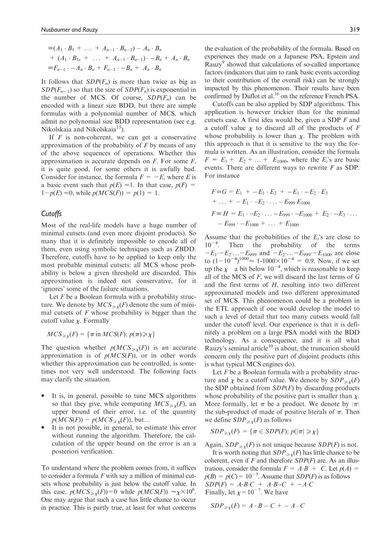
Consider a simplified nuclear power plant model Mconsisting of three safety systems A, B and C. If A fails,then it goes straight to a core damage state (CD). Anyof the safety systems B and C may prevent CD, butboth share a common support system S. The FTLmodel for that power plant is pictured Figure 2.

The master fault tree for the core damage is

FTL(M,C)=�A(B+S) � (C+S)+A

Despite appearances, FTL(M,C) is coherent (it is easyto see that it is equivalent to the formula(B+S)�(C+S) + A). In that case, the minimal cut-sets are easily determined

MSC(FTL(M,C)) =A+ S+B � C:

On large models, success branches are often ignored,i.e. products associated with sequences embed justfunctional events of failure branches. Let M be anevent tree model and C be a consequence. We denoteby FTL+(M,C) the master fault tree associated in thisway with the consequence C in the model M whenignoring success branches. In our example, we have

FTL+ (M,C) = (B+S) � (C+S)+A

It is important to note at this stage that FTL+(M,C) isalways coherent.

The ETL approach

The ETL approach uses relatively large event trees torepresent accident sequences. Typically, several eventtrees are linked together. The ETL approach accountsfor dependencies between plant systems differently thanthe FTL approach does: the fault trees associated withfunctional events are developed so that they do notshare any basic event. At least conceptually, the ETLapproach is obtained from the initial model by succes-sive applications of the Shannon decomposition duringmodel development. Each application corresponds tothe creation of a new functional event and aims to makefunction events independent one another. The processstops when all functional events are independent.

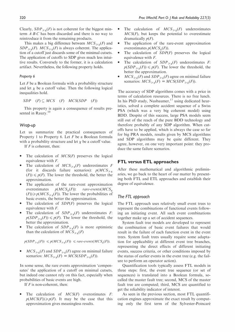
Let M be an event tree model and C be a conse-quence (e.g. core damage, CD). We denote byETL(M,C) the master fault tree associated with theconsequence C in the model M, once developed accord-ing to the ETL approach by adding all CD sequences.In the example of Figure 3 (our simplified nuclearpower plant model), this would be

ETL(M,C)= A+� A � S+� A � �S � B � C

Note that ETL(M,C) can also be obtained, at least con-ceptually, from FTL(M,C), by successive applicationsof the Shannon decomposition and Booleansimplifications

FTL(M,C)=�A � (B+S) � (C+S) +A

=�S � (�A � (B+0) � (C+0))

+ S � (�A � (B+1) � (C+1))+A

=� S � �A � B � C+ S � �A+A

= ETL(M,C)

Figure 2. FTL model for a simplified nuclear power plant.


Once the model expansion is completed, individualsequence frequencies can be easily computed in a two-steps process. First, the top event branch failure prob-abilities are computed, mostly using fault trees. In thesecond step, each of the accident sequence frequenciesis obtained by multiplying the initiating event frequencyby the product of all subsequent event tree branchprobabilities along the respective sequence path. Here,both success and failure branch probabilities can beeasily calculated in the sequence frequency product(because functional events have been made independentof each other). In our example, the exact probabilityp(ETL(M,C)) is calculated as

p(ETL(M,C))= (1� p(A)) � (1� p(S)) � p(B) � p(C)+1� p(A) � p(S) + p(A)

It would be also possible to apply a minimal cutsetsalgorithm to quantify the master fault tree of ETL mod-els. However, it is much more efficient to take advantageof the independence of sequences. Moreover, since faulttrees associated with functional events are now smaller(and pair wisely independent), it is, in general, possibleto assess them exactly with a SDP algorithm, typicallywith BDD, as in Riskman�.18 This is why advocates ofthe ETL approach often claim that ETL is superior toFTL when it comes to PSA/PRA quantification.

In general, there are too many sequences to make itpractical for the analyst to assign in advance end statesfor every sequence. Instead, analysts develop logic rulesfor assigning the end states so that the software canmake the assignments during quantification. Here also,truncation prevails: prefixed sequences with a too lowprobability are discarded.

Although exact, the ETL approach requires muchmore manual work from the analyst to make the func-tional events independent and usually yields less intuitivemodels. The more shared events there are, the bigger theeffort. ETL supporters advocate that this extra work-load comes with a great benefit in terms of system andmodel understanding. We do not enter this debate here.

Strong and weak equivalences betweenmodels

As pointed out in the introduction, a general assump-tion in sciences is that two objects under study can be

considered as equivalent if they cannot be distinguishedwith the observation means at hand. In our case,objects are models, and observation means are quanti-fication algorithms. This leads to the definition of twodegrees of equivalence between models.

Let F and G be two Boolean formulas built over thesame set of basic events and x be a cutoff value

� F strongly entails G at precision x if for any min-term p such that p(|p|) 5x, if p2F then p2G. Fand G are strongly equivalent at precision x, if bothF strongly entails G and G strongly entails F at pre-cision x.

� F weakly entails G at precision x if for any mintermp such that p(|p|) 5x, if p2G then there exists aminterm r4p such that p(|r|) 5x and r2F. Fand G are weakly equivalent at precision x, if bothF weakly entails G and G weakly entails F at preci-sion x.

Strong equivalence means that models agree on all fail-ure scenarios. Weak equivalence means that they agreeat least on minimal failure scenarios. The followingproperty holds, which defines the degree of equivalenceof two models.

Property 7

Let F and G be two Boolean formulas and x be a cutoffvalue. Then:

� If F strongly entails G at precision x, then F weaklyentails G at precision x (weak entailment is coarserthe strong entailment).

� If F and G are strongly equivalent at precision x,then they cannot be distinguished by any correctSDP algorithm: SDP5x(F) [SDP5x(G).

� If F and G are weakly equivalent at precision x,then they cannot be distinguished by any correctminimal cutsets algorithm: MCS5x(F) [MCS5x(G).

The first two points are direct consequences of thedefinitions. For the third one, consider a minterm p

such that |p| is a minimal cutset of F and assume thatp(|p|)5x. Since F weakly entails G, there must be aminterm r such that r4p, p(|r|)5x and r2G. Now,

Figure 3. ETL model for the simplified nuclear power plant.


the same reasoning applies to r. Therefore, there mustexist a minterm s such that s4 r, p(|s|)5x and s2F.Since |p| is a minimal cutset, we must have p= r=s.Therefore, F and G agree on their minimal cutsets atprecision x.

We are now at the heart of our matter and can com-pare FTL and ETL approaches.

A first, nearly obvious, fact is that by discarding suc-cess branches, we make a conservative approximation,which formally established by the following property.

Property 8

Let M be a PSA/PRA model and C be a consequence.Then, FTL(M,C) 4FTL+(M,C).

Proof. Let p be a minterm such that p2FTL(M,C).Then, there must be a sequence S of M that leads tothe consequence C such that p satisfies FTL(S,C). Byconstruction, p must satisfy FTL+(S,C) as well andtherefore FTL+(M,C).

Now what is really interesting to compare is the FTLand ETL evaluation processes, i.e. the two formulas:SDP(ETLx (M,C)) andMCSx(FTL(M,C)). The funda-mental result is the following.

Property 9

LetM be a PSA/PRA model, C be a consequence and x

be a threshold value. Then ETLx (M,C) and FTL(M,C)are weakly equivalent at precision x.

Proof. ETLx (M,C) is obtained from FTL(M,C) bymeans iterative applications of two operations:Shannon decomposition and truncation at precision x.Both operations preserve the weak equivalence, hencethe first result.

In other words, although they may give differentresults, the FTL and ETL approaches agree eventuallyon what is definitely the most important thing: the mostprobable accident scenarios. Moreover, thanks to whathas been established in the previous section, when themodel is coherent and probabilities of basic events nottoo high, the two approaches should give close quanti-tative results.

Corollary. Let M be a PSA/PRA model, C be a conse-quence and x be a threshold value. If FTL(M,C) iscoherent and probabilities of basic events are not toohigh then

p(SDP(ETLx(M,C)’rare� events(MCSx(FTL(M,C)))

Note that one can get rid of imprecision owing to rareevents approximation in several ways. For instance, itis possible to calculate a SDP (a BDD) from the mini-mal cutsets, possibly applying the cutoff x. It is alsopossible to apply the Sylvester-Poincare developmentusing x to prune products with a too low probability.In both cases, the use of cutoffs is probably necessary

in practice to avoid the exponential blow-up of calcula-tion resources.

So, problems, if any, stand in non-coherent models.In the next section, we will discuss where non-coherencemay come from and how to cope with it.

Non-coherent models

In this section, we extend those concepts for the treat-ment of non-coherence model. Non-coherent modelstypically arise when non-monotonic connectives (e.g.negation) are implemented. In this case, a success maycause the top event to occur, indicating how the non-occurrence of an event can cause the top event. In prac-tice, non-coherent models are much more complex toquantify. In fact, large models are, in many cases,impossible to solve using complete negative logictreatment.

In an ETL approach, there is no problem to solveincoherent models exactly. In FTL however, there is noway the exact top event probability can be calculatedfrom the MCS of an incoherent equation. The strate-gies developed in the previous sections break down andan appropriate alternative treatment should be lookedfor. For example, assume the following top event F =A�B +2A�C, with cutsets {AB, C}. There is absolutelyno way the original formula can be retrieved from itsMCS, i.e. the previous algorithm would fail.

Origin of non-coherence

Negation arises naturally as success branches in eventtrees. In fault trees however, the use of negation is morequestionable. It may be used for a variety of differentreasons, and is subject to different algorithmic treat-ments. In fact, there is no reason for quantificationengines to cover all the possible uses of negative logicthat can occur. As will be shown later, such result willoften have no real-life meaning when working in thefailure space. As we shall see, only a few uses of nega-tive logic are pertinent for PSA/PRA.

First, note that FTL models, as found in the nuclearindustry, are largely of coherent nature. Typically, onlya very small fraction of the logical gates makes use ofnegative logic. They may be introduced for a numberof reasons, for example:

� ‘If-Then-Else’ (ITE) operations;� exclude forbidden or impossible configurations;� conditional adaptation of success criteria;� taking credit of failures;� taking credit of success branches;� delete term;� exchanging basic events (specific to CAFTA).

A typical use of negative logic in FTL is as follows: thefault tree model needs to re-test a hypothesis that wasnot queried previously in the attached event tree, lead-ing to the following incoherent ITE operation


F=A � B+� A � C, withMCS(F)= fAB,Cg

As preparatory task for this work, we conducted aninternational survey on the use of negative logic amongpractitioners. We distributed a questionnaire asking forthe different uses of negative logic in nuclear PSA/PRAmodels. Participating countries included Sweden,Finland, France, Germany, Switzerland, Spain andUSA. This survey allowed us to better appraise thenumerous reasons for using negation (major ones arelisted above). Based on the answers from the question-naire, a categorization according to mathematical char-acteristics and treatment by quantification engines wasundertaken. The following three categories were identi-fied and will be discussed in the next sections.

� Exclusion of forbidden or impossible configurations.� Conditional adaptation of success criteria (ITE

operation).� Delete terms.

Exclusion of forbidden or impossible configurations

A typical example of this category is when the analystwants to exclude different configuration alignments.Assume we have a system consisting of two trains Aand B. Each train is taken out of service one day every30 days, with failure probabilities 1023 when operating.As both trains are not allowed to be taken out of ser-vice at the same time by administrative rules, practi-tioners typically implement negative logic to excludethis particular state. In practice, this is modelled usingtwo basic events per train, e.g. PA stands for ‘failure ofthe train A’ and UA stands for ‘train A is out of ser-vice’. The probability of PA and UA are respectively

1023 and 1/30. The unavailability of the whole systemis then modelled as follows

F=(PA �UB � �UA)+ (PB �UA � �UB ) + PA � PB

The above equation is however an approximation,for PA and UA are not independent events. In fact, thedescribed situation can be solved exactly neither by aFTL nor by an ETL approach, since it is a superposi-tion of two distinct states.

Using the rare event approximation to solve suchproblems yields optimistic results in general, as com-bined failures of A and B when no system is in service isneglected. It is possibly to solve such problems exactlythough. To achieve this, quantification engines need toquantify each system configuration individually andsum over all independent configurations so created.This feature is available in Riskman, which can manageup to 32 different configuration states. To the knowl-edge of the authors, no other code offers such a config-uration management feature.

Conditional adaptation of success criteria (ITEoperation)

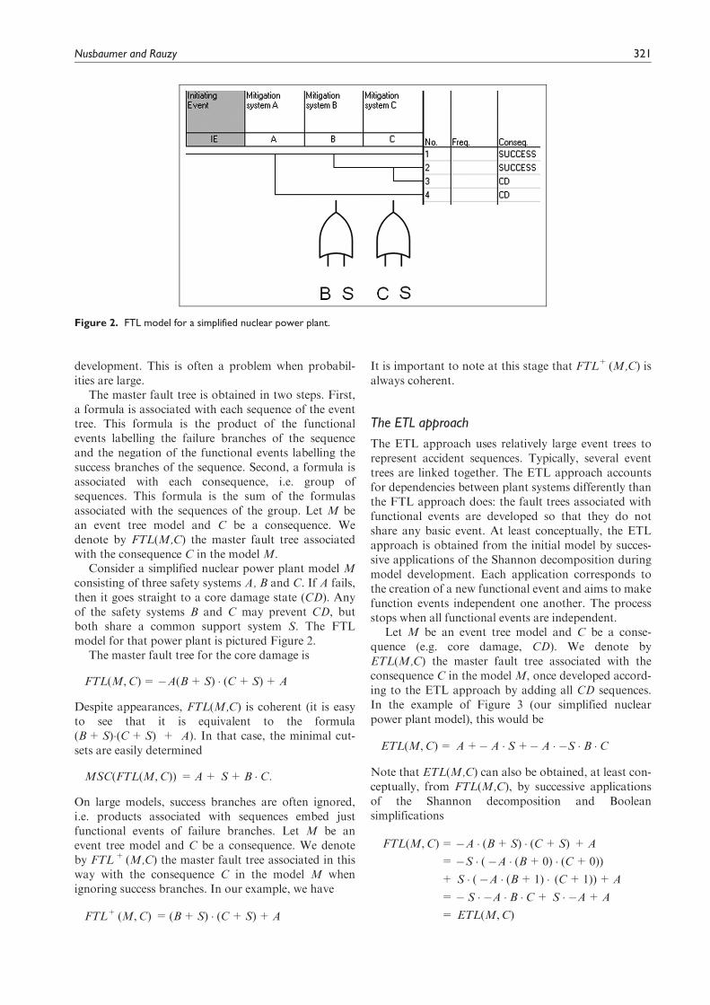
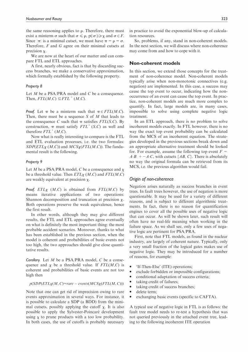
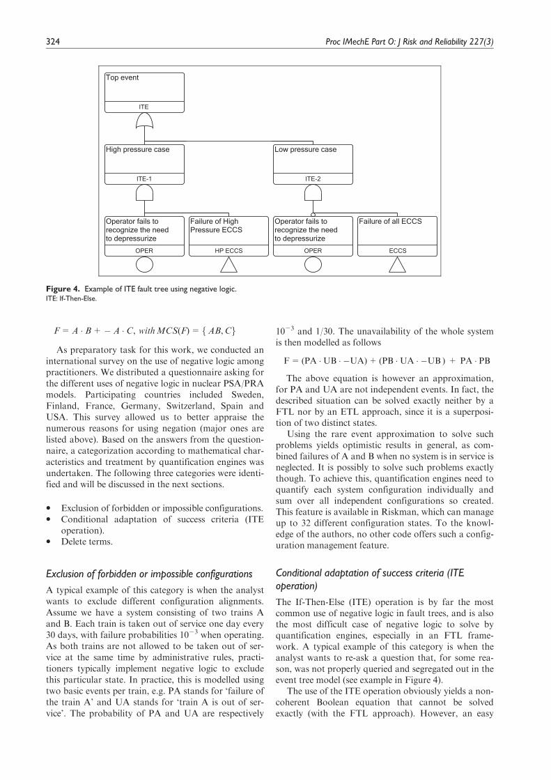
The If-Then-Else (ITE) operation is by far the mostcommon use of negative logic in fault trees, and is alsothe most difficult case of negative logic to solve byquantification engines, especially in an FTL frame-work. A typical example of this category is when theanalyst wants to re-ask a question that, for some rea-son, was not properly queried and segregated out in theevent tree model (see example in Figure 4).

The use of the ITE operation obviously yields a non-coherent Boolean equation that cannot be solvedexactly (with the FTL approach). However, an easy

Top event

ITE

High pressure case

ITE-1

Operator fails to recognize the need to depressurize

OPER

Failure of High Pressure ECCS

HP ECCS

Low pressure case

ITE-2

Operator fails to recognize the need to depressurize

OPER

Failure of all ECCS

ECCS

Figure 4. Example of ITE fault tree using negative logic.ITE: If-Then-Else.


workaround exists that will permit solving the problemexactly: when working in FTL, the attached event treecan be rewritten so that the ITE condition (in ourexample OPER) can be tested in advance in the eventtree. This makes it disjoint (e.g. by application of theShannon decomposition), and coherency is regained (atleast in the fault tree). The event tree ‘absorbs’ the non-coherent parts. The rewriting task can be either doneby the analyst during model development (as in theETL approach), or, more appealingly, automatically bythe quantification engine during event tree pre-process-ing. This comes at a cost however; it generates newfunctional events in the event trees, whose non-coherentsuccess branches need to be calculated, if possiblyexactly.

Delete terms

A delete term operation is simply the task to removeone or many MCS or basic events from the overallresult. A typical example is when the analyst wants toget rid of a specific basic event(s) in a fault tree. Insteadof duplicating the entire fault tree, one typically re-usesan existing fault tree by multiplying (under an ANDconnective) with the negated basic event in question.

Similar to truncation on a FTL framework, deletingbasic events or MCS does not yield incoherent results.The resulting model is, despite appearances, coherent,and the previous results hold.

Exact quantification of success paths in event trees

It may be the case that one wants to assess exactlysequences of events trees that contain success branches.There are different ways of handling these branches(besides calculating a SDP).

Let S = P1�.�Pm�2Q1�.�2Qn be a sequence offunctional events.

A first way to handle this sequence, as implementedfor instance in RiskSpectrum,4 consists in calculatingthe MCS of the formula P1�.�Pm, then those of the for-mula Q1+.+Qn and finally to remove from the

former the minimal cutsets p such that there exists aMCS r of the latter’s such that r4p.

The MCS algorithm proposed recently by Rauzy13

is able directly to handle negative logic. However, inboth cases the quantification passes by the calculationof minimal cutsets and is subject to the problems raisedin the section devoted to algorithmic issues.

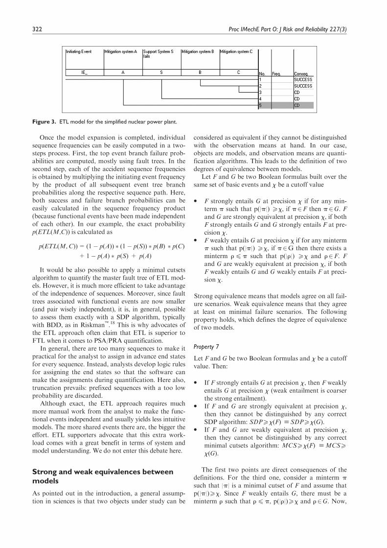
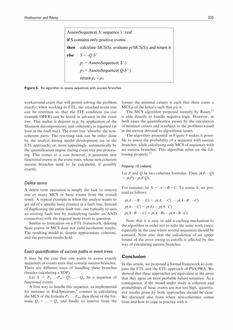
The algorithm presented in Figure 5 makes it possi-ble to assess the probability of a sequence with successbranches, while calculating only MCS of sequences withno success branches. This algorithm relies on the fol-lowing property.11

Property 10 (valiant)

Let P and Q be two coherent formulas. Then, p(P�2Q)= p(P) – p(P�Q).

For instance, let S = A�2B�2C. To assess S, we pro-ceed as follows

p(A � �B � �C)= p(A � �C) � p(A � B � �C)p(A � �C)= p(A)� p(A � C)p(A � B � �C)= p(A � B)� p(A � B � C)

Note that it is easy to add a caching mechanism tothe algorithm in order not to redo the same work twice,especially in the case where several sequences should beassessed. Note also that the calculation of an upperbound of the error owing to cutoffs is affected by thisway of calculating success branches.

Conclusion

In this article, we proposed a formal framework to com-pare the FTL and the ETL approach of PSA/PRA. Weshowed that these approaches are equivalent in the sensethat they agree on most probable failure scenarios. As aconsequence, if the model under study is coherent andprobabilities of basic events are not too high, quantita-tive results given by both approaches should be close.We discussed also from where non-coherence comesfrom and how to cope in practice with it.

AssessSequence( S: sequence ) : real

if S contains only positive events

then calculate MCS(S), evaluate p(MCS(S)) and return it

else S = -Q.S’

p1 = AssessSequence( S’ )

p2 = AssessSequence( Q.S’ )

return p1 – p2

Figure 5. An algorithm to assess sequences with success branches.


Both FTL and ETL approaches clearly satisfy thePSA/PRA needs when applied correctly, i.e. accordingto the algorithmic recommendations of the precedingsections. Generally speaking, the following observa-tions can be made.

� The strength of the FTL approach lies in the factthat the model is (i) complete and (ii) built in anintuitive manner, using immediate cause concept infault trees, and causality chains in event trees.

� The strength of the ETL approach lies in the factthat the model has been initially decomposed in dis-joint functions and that model can easily be solvedexactly.

� The shortcomings of the FTL approach lie in the diffi-culty to solve it exactly (e.g. without approximation).

� The shortcomings of the ETL approach lie in thefact that sequences are made pair-wisely disjoint,leading to (i) a priori truncated models (owing tocutoffs), and (ii) making the model less easy to con-struct and review because it is more distant fromthe architecture of the plant under study than anFTL model would be.

To a large extent, the choice of one or the othermethodology is a matter of taste. Clearly, some opera-tions that are manually performed, such as the creationof a functional event from an internal event of a faulttree, could be advantageously automated or semi-automated.

Conflict of interest statement

The author declares that there is no conflict of interest.

Funding

This research received no specific grant from any fund-ing agency in the public, commercial, or not-for-profitsectors.

References

1. Kumamoto H and Henley EJ. Probabilistic risk assess-

ment and management for engineers and scientists. IEEEPress, 1996. New York USA.

2. NUREG/CR-2300. A guide to performance of probabil-istic risk assessments for nuclear power plants. Washing-ton DC: US Nuclear Regulatory Commission, 1983.

3. Fussell JB and Vesely WE. A new methodology forobtaining cut sets for fault trees. Trans Am Nucl Soc

1972; 15: 262–263.

4. Berg U. RISK SPECTRUM, Theory Manual, 1994.5. Jung WS, Han SH and Ha J. A fast BDD algorithm for

large coherent fault trees analysis. Reliab Engng Sys Saf

2004; 83(3): 369–374.6. Jung WS. ZBDD algorithm features for an efficient

probabilistic safety assessment. Nuclear Engng Des 2009;

239(10): 2085–2092.7. Brace K, Rudell R and Bryant R. Efficient implementa-

tion of a BDD package. In: Proceedings of the 27th

ACM/IEEE design automation conference, 1990. IEEE.

pp.40–45. of the event, publisher, and location of the

publisher. Orlando, Florida, USA, June 24–28, 1990.

IEEE Computer Society Press 1990, ISBN 0-8186-9650-

X, New York, USA.8. Rauzy A. BDD for reliability studies. In: Misra KB (ed.)

Handbook of performability engineering. Elsevier, 2008,

pp.381–396. London, England.9. Epstein S and Rauzy A. Can we trust PRA? Reliab

Engng Sys Saf 2005; 88(3): 195–205.10. Rauzy A. Mathematical foundation of minimal cutsets.

IEEE Trans Reliab 2001; 50(4): 389–396.

11. Valiant LG. The complexity of enumeration and reliabil-

ity problems. SIAM J Comput 1979; 8: 410–421.12. Minato S. Zero-suppressed BDDs for set manipulation

in combinatorial problems. In: Proceedings of the 30th

ACM/IEEE Design automation conference, 1993,

pp.272–277. Dallas, Texas, USA, June 14–18, 1993.

ACM Press, New York, NY, USA 1993 ISBN 0-89791-

577-1 Reference 13. June 23–27, Helsinki Finland, IAP-

SAM, USA, ISBN: 978-1-62276-436-5.13. Rauzy A. Anatomy of an efficient fault tree assessment

engine. In: Virolainen R (ed.) Proceedings of international

joint conference PSAM’11/ESREL’12, 2012, Helsinki.14. Rauzy A. New algorithms for fault trees analysis. Reliab

Engng Sys Saf 1993; 59(2): 203–211.15. Nikolskaia M and Nikolskaia L. Size of OBDD represen-

tation of 2-level redundancies functions. Theoret Comput

Sci 2001; 255(1–2): 615–625.16. Duflot N, Berenguer C, Dieulle L, et al. How to build an

adequate set of minimal cut sets for PSA importance

measures calculation. In: Stamatelatos MG and Black-

man HS (eds) Proceedings of the 8th international confer-

ence on probabilistic safety assessment and management,

2006. May 14–18, 2006, New Orleans, Louisiana, ISBN-

10: 0791802442| ISBN-13: 978-0791802441, Cdr17. Nusbaumer O. Analytical solutions of linked fault tree

probabilistic risk assessments using binary decision dia-

grams with emphasis on nuclear safety applications. Zur-

ich: ETH Zurich; 2007.18. Wakefield DJ, Epstein SA, Xiong Y, et al. Riskman�,

celebrating 20+ years of excellence! In: Proceedings of

PSAM’10 conference, 2010, Seattle. June 7–11, Seattle,

USA, IAPSAM, USA


Documents

Proc IMechE Part O: J Risk and Reliability Fault tree ...nusbaumer.tripod.com/...FaultTreeLinkingVersusEventTreeLinking.pdf · Fault tree linking versus event tree linking approaches: