Embed Size (px)
Citation preview

Department of Automatic Control
Probabilistic Lane Association
Elin Dahlin

Msc ThesisISRN LUTFD2/TFRT--5937--SEISSN 0280-5316
Department of Automatic ControlLund UniversityBox 118SE-221 00 LUNDSweden
© 2014 by Elin Dahlin. All rights reserved.Printed in Sweden by Media-TryckLund 2014

3
Abstract Lane association is the problem of determining in which lane a vehicle is currently driving, which is of interest for automated driving where the vehicle must understand its surroundings. Limited to highway scenarios, a method combining data from different sensors to extract information about the currently associated lane is presented.
The suggested method splits the problem in two main parts, lane change identification and road edge detection. The lane change identification mainly uses information from the camera to model the lateral movement on the road and identifies the lane changes as a relative position on the road. This part is implemented with a particle filter. The road edge detection enters radar detections to an iterated Kalman filter and estimates the distances to the road edges.
Finally, a combination of the filter outputs makes it possible to compute an absolute position on the road. Comparing the relative and absolute positioning then leads to the desired lane association estimate.
The results produced are reliable and encourages to continue approaching this problem in a similar manner, but the current implementation is computationally heavy.

4

5
Populärvetenskaplig Sammanfattning Som ett steg mot framtidens förarlösa fordon behövs metoder för att öka förståelsen av omvärlden. En bit i det stora pusslet är att kunna identifiera i vilken fil ett fordon kör, till en början begränsat till motorvägskörning. Det är vad detta projekt handlar om, där uppgiften är att undersöka möjligheterna att få ut information om filtillhörighet på ett robust sätt med tillgänglig data.
En modern lastbil innehåller stora mängder elektronik för att styra och kontrollera funktionen. Lagkrav om exempelvis nödbroms har infört radar och kamera som standardutrustning, och data som dessa sensorer kontinuerligt samlar in kan användas till att ta fram en mängd olika information.
Från en kamera kan man få information om vägmarkeringar och deras sträckning. Genom att kombinera kameradata med lastbilens acceleration i lateral riktning, kan den laterala rörelsen över vägen modelleras. Med fokus på korsning av väglinjer kan filbyten identifieras.
Radardetektioner kommer från alla objekt framför ett fordon; andra fordon, vägräcken, vegetation längs vägen, osv. Genom att sortera ut detektioner från vägräcken kan avståndet till vägens ytterkanter skattas.
Den information som fås från kamera och radar kan sedan kombineras till en skattad filtillhörighet. De resultat som presenteras i den fullständiga rapporten kan med bra resultat verifiera att detta är ett möjligt angreppssätt för att lösa det presenterade problemet.

6

7
Acknowledgements First of all, I would like to thank the people who helped and guided me during my time at Scania, especially my supervisor Pär Degerman with his never-failing patience and expertise. Christoffer Norén also deserves recognition for all the practical help with understanding and retrieving data. I will also never forget the other employees and thesis students, who would always be up for a refreshing coffee and conversation.
I would also like to thank my supervisor and examiner at LTH, Bo Bernhardsson, who has been of great importance with his guidance and perspective.
Finally, I would like to thank my family and friends, without whom nothing would be possible.

8
Contents 1. Introduction ............................................................................................... 10
1.1 Background .......................................................................................... 10
1.2 Purpose and Goals ............................................................................... 12
1.3 Methodology ........................................................................................ 12
1.4 Report Outline ..................................................................................... 13
2. Related Work ............................................................................................. 14
3. Truck and Sensor Setup ............................................................................. 16
3.1 Internal Communication ...................................................................... 16
3.2 Camera Data ........................................................................................ 19
3.3 Radar Data ........................................................................................... 20
3.4 Map Data ............................................................................................. 21
4. Theory ........................................................................................................ 22
4.1 Sensor Fusion ...................................................................................... 22
4.2 Filters ................................................................................................... 24
4.3 Kalman Filter ....................................................................................... 24
4.4 Particle Filter ....................................................................................... 28
4.5 Change Detection – The CUSUM Algorithm ..................................... 34
5. Implementation .......................................................................................... 36
5.1 System Overview ................................................................................. 38
5.2 Logged Data ........................................................................................ 39

9
5.3 Lane Change Identification ................................................................. 41
5.4 Road Edge Detection ........................................................................... 47
5.5 Lane Association ................................................................................. 52
6. Results ....................................................................................................... 55
6.1 Lane Change Identification ................................................................. 55
6.2 Road Edge Detection ........................................................................... 69
6.3 Lane Association ................................................................................. 74
6.4 Final Performance ................................................................................ 79
7. Discussion .................................................................................................. 81
7.1 Model Critique ..................................................................................... 81
7.2 Filter Critique ...................................................................................... 82
7.3 Data Selection ...................................................................................... 83
7.4 Structure of Computations ................................................................... 84
7.5 Computational Complexity .................................................................. 84
7.6 Conclusion ........................................................................................... 84
7.7 Future Research ................................................................................... 85
8. References ................................................................................................. 86

10
1. Introduction This master thesis presents a way of determining in which lane a vehicle is driving in a highway scenario. The project was performed at Scania, using information from currently available sensors on Scania trucks, especially radar and camera data is essential for this application.
The project was an overall success, the implemented system can produce stable and robust lane estimates for data recorded on highways.
1.1 Background Increasingly higher requirements on fuel economy and safety motivate the development of more advanced vehicles. The automotive industry puts great effort in research to adapt to the new demands on the market.
Heavy-duty vehicles contribute greatly to the carbon dioxide emissions to the atmosphere, an approximation by the European Commission is a quarter of the total emissions from road transport and 6 % of total carbon dioxide emissions in the European Union [1]. This has negative impact on the environment and oil is a limited resource. Fuel costs stand for about 35 % of the total cost for a modern haulage contractor [2], a decrease in fuel consumption is strongly economically motivated from their perspective. Modern systems can teach truck drivers how to drive more environmentally friendly, but full or partial automation has potential to further decrease fuel consumption. One example of this is platooning [3], where communicating vehicles autonomously drive closely together to decrease air drag and thereby fuel consumption.
Safety is potentially an even more important issue to consider in this case. In Sweden, Trafiksäkerhetsverket has a vision of zero deaths and serious injuries in traffic [4], an idea that has also gotten attention internationally. Traffic related deaths have been decreasing steadily over the last decades as the safety in vehicles has increased [5].
11
An older report concludes that human factors alone were the definite or probable cause in 57 % of all accidents and a contributing factor in over 90 % of the cases [6]. Essentially, this is caused by the limited information processing capabilities, which is based on the perception, attention and memory of the driver. These abilities can also be impaired by alcohol, fatigue or other distractions.
The only way to completely remove this risk factor is to rely on an automated system that cannot be affected by this kind of external factors and ideally performs perfectly in any situation.
In order to make it possible to automate vehicles, they must be able to perceive their environment, understand the current situation and take deliberated action.
In the automotive industry, the development of a large number of systems assisting the driver is an important area and software in general is of increasing importance. For some applications, software can reduce costs by replacing expensive sensors [7]. These new, somewhat intelligent functions, are grouped under the name Advanced Driver Assistance Systems, ADAS [8]. Some examples of currently available systems are adaptive cruise control, emergency brake systems and in-vehicle navigation systems. The main purpose of these systems is to increase safety by assisting the driver in some situations.
Figure 1 Scania Truck on the Road [9]
12
Scania is a major manufacturer of heavy trucks and buses as well as industrial and marine engines. The main business is heavy trucks with 61,000 sold units in 2012 around the world, Figure 1 shows one of these heavy trucks. Scania is a global company with almost 40,000 employees in over 100 countries. Headquarters and research and development are located in Södertälje [2].
Several projects at Scania develop different kinds of ADAS and with them related software. The FFI project iQMatic is a collaboration between Scania, KTH, Autoliv and LiU and has as a goal to deliver fully autonomous trucks to a mining environment where the trucks can transport overburden to a dumping site.
1.2 Purpose and Goals As a part of the iQMatic project, this project explores further possibilities of using existing sensors to extract more information about the current situation. Specifically, the purpose of this project is to examine the possibilities of extracting information about in which lane a vehicle is currently driving from data available from radar sensors and camera, available in trucks on the market today. This is one of the steps for increasing the vehicles awareness of the surroundings and this information is of importance for future systems involved with automated driving.
The goal of this project is to formulate a stable lane association method with possibilities to use in real-time for future needs in automated driving. The lane association estimate should be reliable in a highway situation independent of situational variations.
1.3 Methodology An initial review of literature, scientific papers and dissertations was conducted to give an overview of similar work on the area. Theory, especially for different filtering algorithms, was also revised.
Based on the review results, models and filters were developed in a modular manner, where different functionality were put in individual parts to keep complexity down and allow for change of strategy. Simulations were made, for each module, with real logged data and evaluated by performance and comparison with desired output. The evaluation results lead to improvements in models and filter tuning, and new simulations in an iterative manner. The final results are the collaborative results from all modules working together.
All modelling and simulations are done in MATLAB [10].
13
1.4 Report Outline The report is divided in 6 chapters. After this first introductory chapter, the content can be briefly summarized per chapter as follows.
Related Work – Summary of similar work done on the area with focus on related approaches and methods.
Truck and Sensor Setup – An overview of the communication in the truck, the sensors used as data sources and the format of the data the sensors produce.
Theory – Background about sensor fusion in vehicles, theory about different filters and implementation specific design alternatives with focus on what is implemented.
Implementation – Detailed description on implementation and the design choices presented per function.
Results – Results from simulations focusing on relating back to design choices and step by step getting to the final associated lane estimate.
Discussion – The method and results are critically discussed and improvements and future possibilities are suggested.

14
2. Related Work This chapter gives a brief overview of the research topics related to the area. There has been little research with the single ambition to identify the current lane, as this information itself is not very useful. Some areas facing similar problems are also presented, as well as some similar approaches to problems of different character.
Some of the concepts mentioned here will be explained further in the theory section as they are relevant for the project. It might be useful to read this section after the rest of the report, both for increased understanding of the work done and better perspective on the comparison to the similar projects.
Lane detection is a topic which has received quite a lot of attention, the camera and image processing is central for this purpose. Normally, included in this term is localization of the road, the determination of the relative position on the road and some kind of analysis of the vehicles heading on the road. One suggestion for real-time lane detection is given by [11], where all focus is on the image processing as the camera is the only source of information.
Lane departure warning systems use lane detection to determine when vehicle is about to leave the lane without a turn signal being active in that direction. If this is about to happen, the system can either indicate this to the driver as a warning or actively take control of the vehicle and prevent the lane change [12].
Typically, lane departure warning systems rely heavily on visual information, and are thus sensitive to roadway conditions. A multi-sensor fusion approach presented in [13], where GPS, inertial sensors and high-accuracy maps are used to assist the vision-based system with a backup lateral offset to the lane markings.
One of the more similar approaches to this project found in theory is [14], here the road estimation is of as much interest as the lane association. Both rely only on radar, and no camera signals are used at all. Guard rails and the tracking of other vehicles on the road are the important sources for information. The lane

15
association is done looking at the position relative to the road and the other vehicles, it is also closely connected to the estimated course of the road.
Guard rails are also in focus in [15], where guard rails and other vehicles are identified with camera and radar sensor fusion. The focus is on visually tracking vehicles, detecting the guard rails is mostly done to increase the performance of the tracking.
Another challenging problem is to estimate the course of a road in rural environments, one example of how unmarked and winding rural roads can be detected is given by [16]. Here, guard rails and lane markings heavily relied on in highway scenarios cannot be assumed to exist. The idea is to extend the more frequently used image-based lane recognition with evaluation of 3D information from stereo vision cameras or imaging radar. Several different filtering approaches were evaluated, and a combined Kalman particle filter is proposed as best choice. A slightly different approach for the same problem is presented in [17], where each road feature is tracked individually.
Finally, an approach combining relative and absolute positioning estimates is given by [18], where the application is a simultaneous localization and mapping problem.
These are some examples of the wide-ranging work used as reference and inspiration for different parts of the project.

16
3. Truck and Sensor Setup A modern truck is equipped with a large numbers of sensors, mainly for being able to control the basic functionality, such as engine, brakes and gearbox. The extended legal demands and safety goals have forced the introduction of long distance radars and a forward-looking camera. These existing sensors are what this project mainly uses as input, relevant information about the sensors and the produced data is presented in the following sections.
All data produced by sensors, as well as any other information being communicated within the vehicle, is sent on the vehicle internal CAN-network. Within all original equipment manufacturers, OEMs, large amounts of data transmitted on the network on different trucks on the road is logged for development purposes and diagnostics. Throughout this project, this logged CAN-data has been used as input for the models and filters. An overview of the internal communication follows.
3.1 Internal Communication In a truck there can be as many as 20 different electrical control units, ECUs, communicating internally to make the truck function in a normal way. An ECU can have a number of sensors and actuators connected to it and it is normally responsible for some functionality, where engine control is one of the more complicated examples.
The internal communication standard in the automotive industry is using controller area networks, CAN, which was created by Bosch in 1983 and has been used widely in vehicles since [19]. A CAN frame has the format seen in Figure 2.
Figure 2 CAN Frame [20]

17
The basic CAN frame depicted above consists of several parts [20];
• Start Of Frame, SOF, indicates the beginning of the frame • The identifier is also the arbitration field, see below, and contains
information about the frame content • Remote Transmission Request, RTR, is used to distinguish between the
data frame and the data request frame • IDentifier Extension, IDE, is used to distinguish between the CAN base
frame and the CAN extended frame • Data Length Code, DLC, indicates the number of bytes in the following
data field • Data is the actual message transmitted and can be up to 8 bytes long • Cyclic Redundancy Check, CRC, is a calculated checksum that
guarantees the integrity of the frame • ACKnowledge, ACK, is transmitted as a recessive bit and should be
overwritten by receivers with a dominant bit to indicate that the message has been received
• End Of Frame, EOF, indicates the end of the frame • Intermission Frame Space, IFS, is the smallest number of bits separating
two consecutive messages
The CAN message identifier is indicating the content of the message as well as the priority on the bus. In case of bus access conflicts, the arbitration mechanism handles these, allowing the message with the lowest binary identifier and highest priority to be transmitted [21]. Other units will be listening until the priority of their message allows transmission, and any unit interested in the specified content can read a message when it is on the bus [20].
Errors are detected in five different ways in the standardized protocol [21].
• Bit monitoring – Each transmitter monitors the bus level and signals an error if the bus level does not match the transmitted signal
• Bit stuffing – After transmitting five identical bits, a node will always transmit an opposite bit, that will be neglected by the receiver but can be used for error detection
• Frame check – Checks that the fixed bits on the frame have the expected values

18
• ACK check – All receivers should send an ACK during this part of the message frame, if this is not detected by the transmitter an error has occurred
• CRC – Each receiver calculates the checksum for the message received and compares to the CRC in the message
In case an error is detected, the incorrect message will immediately and automatically be retransmitted. This leads to high data integrity and short error recovery times compared to many other network protocols [21]. The mentioned error detection is only for the two lower OSI layers [22], which are covered by the standard, additional error detection could be implemented in higher layers in applications.
Regarding timing, it is hard to generally guarantee that messages arrive at a certain time. Scheduling and response-time analysis can be done for specific cases, see [23], but a general approach when designing the communication structure is to make the bus fast enough and the number of connected nodes small enough, the delays are then expected to be sufficiently small.
The ECU’s are in Scania trucks connected to three different buses, ordered by priority, see Figure 3 for an overview. Essential systems communicate on the red bus, such as the previously mentioned engine management system, EMS, or the brake management system, BMS. Less critical systems communicate on the yellow bus, examples here are the instrument cluster system, ICL, and the all-wheel drive system, AWD. The least crucial information is put on the green bus, such as the climate control, ACC. These buses are connected at a gateway unit, called the coordinator, COO, which is distributing messages required on several buses and also does some processing itself [21]. With the addition of more sensors and ECU’s for the development of more advanced functionality in the vehicles, another CAN-bus is added. An overview of a typical truck setup can be found in the image below.

19
Figure 3 Overview of CAN structure in typical Scania truck. ECUs are connected to one of three buses, sorted by importance. The coordinator unit distributes information between buses. Scania internal image.
For more details the two lower OSI layers, which the CAN protocol standardizes, refer to [24], or more details on applications of CAN in different types of vehicles, refer to [21].
3.2 Camera Data The forward-looking camera is a normal mono-camera bought by Scania from a supplier as a black-box component. It is unfortunately delivered without any formal documentation and the performance is agreed on by a constant undocumented dialogue, what is mentioned in this section is based on experience and general practice.
The supplier is responsible for some camera internal image processing and feature extraction, before publishing data on the CAN-bus. Typically, this kind of lane detection systems is based on Hough-transform of which there are plenty of examples in literature, see for example [25]. The extracted features from the image processing are published on the CAN-bus at a frequency of about 12 Hz.
The camera detects, among other things, the closest lane marking to the left and right, and presents this information on the bus as coefficients for a third degree polynomial. Each time new data is available from the camera, a triplet containing value, time and quality of the value is posted. The quality is an index
20
from 0 to 3, where 3 indicates excellent quality and 2 good quality. Data marked with 0 or 1 is not deemed to be of good enough use for this application.
The general quality and reliability of the camera signals is determined from frequent use at Scania to be quite high. There are a few situations known to be problematic; for example snow covering lane markings or wet road in combination with the low standing sun causing reflections. In other words, situations which cause the contrast between lane marking and road to become too low are problematic since the image processing relies on the contrast to extract the information. Fortunately this does not apply to a very large number of situations. Problems could also occur if the windshield is very dirty, with dirt directly blocking the view of the camera.
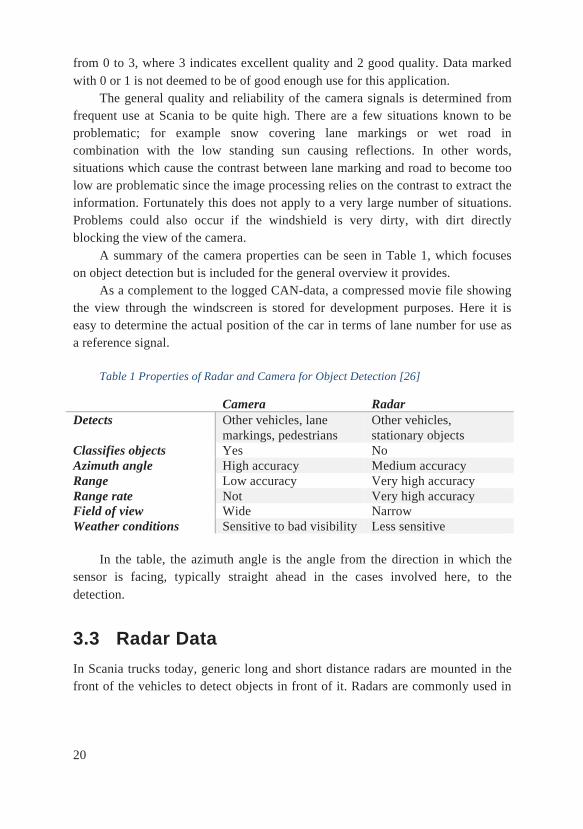
A summary of the camera properties can be seen in Table 1, which focuses on object detection but is included for the general overview it provides.
As a complement to the logged CAN-data, a compressed movie file showing the view through the windscreen is stored for development purposes. Here it is easy to determine the actual position of the car in terms of lane number for use as a reference signal.
Table 1 Properties of Radar and Camera for Object Detection [26]
Camera RadarDetects Other vehicles, lane
markings, pedestrians Other vehicles, stationary objects
Classifies objects Yes No Azimuth angle High accuracy Medium accuracy Range Low accuracy Very high accuracy Range rate Not Very high accuracy Field of view Wide Narrow Weather conditions Sensitive to bad visibility Less sensitive
In the table, the azimuth angle is the angle from the direction in which the sensor is facing, typically straight ahead in the cases involved here, to the detection.
3.3 Radar Data In Scania trucks today, generic long and short distance radars are mounted in the front of the vehicles to detect objects in front of it. Radars are commonly used in

21
automotive applications because of the high reliability and accuracy, and low sensitivity to weather and dirt, see Table 1.
The long-distance radar can detect several objects at each measurement instant, the update frequency is 20 Hz with the current setup in the truck. The detections each have information about distance, velocity and acceleration in the direction of detection and an angle from the longitudinal direction of the truck (and radar) that relates the previously mentioned parameters to the truck coordinate system. These signals are considered to be the raw radar signals.
Each of the detections are also classified as true or false for the following categories; movable fast, movable slow and moving. The movable categories indicate if an object is movable, where other vehicles are examples of fast movable objects. The moving category, on the other hand, indicates if an object is currently moving. These categories are evaluated separately; an object identified as a fast movable object, could thus be known to have stopped, and moving would be false.
The raw signals are processed and grouped into targets that different applications can use for a variety of purposes. One important use is tracking objects, where the classification of these objects as moving or static is important.
When determining distances to road boundaries the static detections along a road, such as from guard rails, are of interest. This implies that it is suitable to use the raw radar signals for this application. There are methods suggested for detecting extended objects, instead of working with the individual measurements, refer to for example [27] in the static case and [28] in the dynamic case, but these will not be elaborated further here. The basic idea, however, is to associate the individual detections with any number of objects with certain dynamic behavior and track them over time.
3.4 Map Data It can be assumed that some other information is available to a vehicle on the road which is associated to the location, this is called map data. This map data includes information regarding topology, speed limits and total number of lanes in the current road segment to mention a few examples.

22
4. Theory This chapter introduces the necessary theory on which this project is based. Initially the concept and benefits of sensor fusion is presented, this is followed by a brief introduction to general filter theory and then a presentation, in more detail, of the filter variants used. Finally a practical approach for change detection is presented.
4.1 Sensor Fusion Sensor fusion is a term used for the combination of data from different sensors in a way that the final data in a sense contains more information than the data from the original sources individually [26] [29]. Common ways of handling this kind of fusion are different statistical approaches, such as least squares methods, maximum likelihood methods and a variety of Bayesian approaches [30].
As previously mentioned, the automotive industry finds the sensor fusion approach very desirable as a way of replacing expensive sensors with more intelligent ways of using cheaper alternatives [7]. Many ADAS use or could use the same state estimates, Figure 4 shows how a central fusion could be structured in the future.

23
Figure 4 Sensor Fusion Vision [7]. Sensors on the left side provide information about, for example, acceleration, position and speed to the sensor fusion. From the data provided by the sensors, information can, using sensor fusion, be extracted to be used to navigate, track objects or acquire situational awareness for a few examples. This is a vision of how these systems can be structured in the future, centralizing the sensor fusion and sharing the extracted information.
The figure also shows common sensors providing input and typical output data.
Sensor fusion can be implemented in a centralized or decentralized fashion. Centralized fusion means that one filter is developed with all available measurements as input. Decentralized fusion, on the other hand, implies that different filters handle different measurement inputs, and the fusion uses only the filter output [30].
One example of a way of combining information from different sources, as mentioned in [30], is to use weighted least squares, WLS. This would give a combined result of value, x, and variance, P, according to the following.
Equation 1 Fusion of Two Independent Estimates

24
The result is simply a linear combination of the two estimates, weighted by their quality given by the inverse variances. This assumes the estimates are independent.
4.2 Filters Recursive Bayesian estimation is a common approach for solving estimation problems in a probabilistic manner. It is a general method, and some of the fundamentals will be presented in this section [31].
Initially, assume there is a model of the following form,
Equation 2 General Bayesian Model
This means that there is a probability distribution that can predict the state xand measurement z with some degree of certainty. The k index indicates the current time step, and k+1 the closest following. Given the model above, the filtering density and the prediction density one step ahead can be expressed according to the following recursive relations, known as the measurement updateand state update.
Equation 3 General Bayesian Prediction
The presented equations in this section summarizes the basics in Bayesian filtering, they will be referred to as the filtering theorem [32]. The special case of the theorem when the model is linear and the noise is white and Gaussian, is the well-known Kalman filter, presented in the following section.
4.3 Kalman Filter The Kalman filter, KF, is an efficient recursive filter for linear dynamic systems based on a Bayesian model. It has numerous applications in a large variety of fields and is of great importance in sensor fusion because of its flexibility [30].

25
For linear Gaussian systems, the KF computes the posterior distribution exactly by updating finite-dimensional statistics recursively [33]. The KF is optimal in the sense that it gives the exact posterior density, given that the system is linear and completely known and the noise is white [31].
TheoryThe KF is well known and commonly used, the filter derivation below follows [30]. The filter estimates the states x and measurements z in a linear state space model given by
Equation 4 Kalman Filter Model
Here u is the control signal, v is the process noise and e the measurement noise. The F matrix represents the process model and how the states evolve over time, the G matrices indicates how the control signal and the noise affects the different states, the H matrix is the measurement model and shows which states can be measured and how, and the D matrix shows the direct component of the control signal on the expected measurements. Q and R are the covariance of the process and measurement noise respectively.
Initial state and covariance can, as implied by above, be expressed as
Equation 5 Kalman Filter Initializations
In its standard form, the filter based on the given state space model can be divided in two steps and expressed in the following recursive algorithm.
Measurement update:
Time update:

26
Algorithm 1 General Kalman Filter Algorithm
A suggested way to structure the computations is to define the innovation
Equation 6 Innovation
the innovation covariance
Equation 7 Innovation Covariance
and the Kalman gain
Equation 8 Kalman Gain
The measurement update can with these definitions be written
Equation 9 Alternative Measurement Update
Again, this assumes a linear model with white Gaussian noise.
Kalman Filter Variants There are several variants of the KF, all considered classical approaches to Bayesian filtering, which makes it possible to solve many different types of problems. Essentially, the basic version requires a linear model and can only produce a unimodal posterior distributions, but the variants are more flexible [33].
The Extended Kalman filter, EKF, is an approach that takes a nonlinear, non-Gaussian model and applies the KF to the linearized model with Gaussian noise. The linearization is done around the previous estimate, typically with the first, sometimes also including second, order terms of the Taylor expansion. There are no guarantees that the linearization and noise assumptions will give good results, however, in some applications where nonlinearities are small and the true posterior is unimodal, this works well [33].

27
The Unscented Kalman filter, UKF, uses a few carefully selected so called sigma points to represent the unimodal Gaussian distributions. The UKF handles nonlinearities better than the EKF, but there are still limitations [33].
The Gaussian sum Kalman filters, GS-KFs, is a group of approximative filters that describes the posterior distribution as a sum of Gaussians, thereby allowing multimodal posteriors. These filters recursively form the Gaussian posteriors, essentially resulting in the parallel operation of several Kalman filters [34].
The Iterated Kalman Filter With a large number of independent measurements per time step, it is possible to apply an iterated Kalman filter, IKF. This is a variant of the KF which uses the basic theory but allows for any number of measurement updates between two time updates, instead of continuously alternating the two as the basic KF suggests. Intuitively it is reasonable to accept that two measurements with zero time difference can update the filter without a time update in between, a formal proof can be derived from the information filter, refer to [30].
Specifically, this means that the standard KF measurement update equations, after initializing
Equation 10 Iterated Kalman Filter Initializations
for each of total M measurements i = 1, 2, …, M will appear as follows
Equation 11 Iterated Kalman Filter Measurement Update
The final measurement update step is then
Equation 12 Iterated Kalman Filter Final Measurement Update Step

28
The order in which the measurements are added to the filter does not impact the final result.
Outlier Detection and Rejection Algorithm In order to avoid having unwanted measurements disturbing the filter performance outliers should be filtered out before adding measurements to the filter. This can be done in many ways, basically any hypothesis where a measurement can be tested as an inlier/outlier, and possibly rejected depending on the result, would be sufficient to increase performance if the measurement signal has outliers [30].
StabilityThe Kalman filter is sensitive to model imperfections and deviations in the noise covariance from the true values. For numerical stability, the covariance matrix Pmust be positive-definite [30].
4.4 Particle Filter The particle filter, PF, is a stochastic method based on Monte Carlo integration and is also known as sequential Monte Carlo, SMC [26]. It is an alternative to the commonly used KF in cases when the model is very nonlinear, beyond where the “linearized” extended Kalman filter or other variants apply. The earliest mentions of the PF are from the 1950s, but only since the publication of [35] in the 1990s when computational power started becoming more available, did this computationally complex filter gain recognition. The positioning problems of vehicles in real-time has been one of the big areas of application for the PF. Extensions of the positioning problem are algorithms for simultaneous localization and mapping, SLAM, an important development and application based on the PF [33].
The PF is approximating a posterior distribution of the state given the measurements , based on a set of N samples. These samples are called particles and each has an associated weight w. For each time step, all particles are sent through the process model, read by the measurement model and assigned weights with a likelihood function on how good approximation of the true measurements that they make. Resampling, choosing a new set of particles from the old set, can optionally be used to keep up the quality of the particles. The steps that the filter iterates through are thus, again according to [30]

29
1. The measurement update: Modify the weights according to the likelihood function of the difference between observed and predicted measurements.
2. Resampling: Take N new samples of the state from the existing set of particles.
3. The time update: Simulate a trajectory from one measurement time to the next using the dynamic model.
The approximated resulting posterior distribution is for each time step the discrete set of particles representing the estimated state
Equation 13 Particle Filter Approximated Posterior
where (u) is Dirac’s delta function [30].
TheoryThe filter theory in this section is based on [30]. The PF can be applied to any nonlinear non-Gaussian model, in general form given by
Equation 14 General Model for Particle Filter Application
There are no restrictions on the probability density functions (PDF) of the process and measurement noise, but they are assumed to be known. The general form of the PF algorithm follows.
First of all a proposal distribution must be chosen, as well as a resampling strategy and the number of particles N.
Initialization: Generate , i = 1, …, N and let .Iteration: For k = 1, 2, …
1. Measurement update: For i = 1, 2, …, N,
where the normalization weight is given by

30
2. Estimation: The filtering density is approximated by
and the mean, considered to be the filter estimate, is approximated by
3. Resampling: Optionally at each time, take N samples with replacement from the existing set of particles where the probability to take sample i is
and then set the new particle weight .4. Time update: Generate predictions according to the proposal distribution
and compensate for the importance weight
Algorithm 2 General Particle Filter Algorithm
It is possible, and common, to combine the two weighting steps. This section presents the general form of the particle filter, there are several
variants and extensions, some of which are presented in detail in [31].
Selection of Proposal Density To be able to implement a filter according to the principle outlined above, the proposal density q must be selected. Principally, it can be freely selected as any kind of distribution, typically Gaussian, naturally affecting the approximation and therefore the performance negatively with a “bad” selection.
Following the practice in [32], a more straightforward way of looking at the proposal density is presented in this section, valid in the case of a SIR filter, see section Resampling on page 32. This version of the PF represents making a set of design choices and is commonly known as the bootstrap filter. The important aspects are that in order to resample, a proposal density and a corresponding importance weight are required.
According to the basic filter theory, see Equation 3, here repeated, we have

31
which would suggest
Equation 15 Relationship between Target Density, Importance Weight and Proposal Density
These terms can be interpreted as the target (filtering) density, the importance weight and the proposal density respectively. Following again the basic theorem in section 4.2 and the interpretation of the equation above,
Equation 16 Interpretation of Proposal Density
This implies that the proposal density can be chosen as
Equation 17 Suggestion for Proposal Density
This means that the particle predictions can be made by simply updating the particles from the previous time step using the process model. Formally, for each particle
Equation 18 Formal Notation of Particle Update
Or using the model notation introduced in the Theory section on page 25

32
Equation 19 Particle Update with Model Notations
As mentioned, this simplification makes the implementation more straightforward and is less computationally expensive than sampling from a given distribution. This is the most common version of the PF, and it performs well when the signal-to-noise ratio, SNR, is small [33].
Number of Particles The most important design choice is the number of particles used. The tradeoff is between getting a good representation of the full spectrum of the posterior PDF and the computational complexity a large number of particles causes [33].
Effective Number of Samples Looking at a PF, it is important to avoid something called sample depletion. This means, that without any countermeasures, over time all particles except for a very few will have negligible weights. To indicate the degree of depletion the effectivenumber of samples is introduced as
Equation 20 Effective Number of Samples
where a computable approximation is
Equation 21 Approximation of Effective Number of Samples
This means that the effective number of samples can be interpreted to be at its largest equal to the total number of samples when the weights are equal, and at its smallest equal to 1 when all particles except one has zero weight [30].
ResamplingResampling avoids the sample depletion problem by, as previously mentioned, selecting a new set of particles from the highest weighted particles of the old set. It is here important to make sure that the new set still represents the distribution in a good way, not selecting too few particles to represent the entire range since

33
throwing away particles essentially means throwing away information. This problem is called sample impoverishment, and in the extreme case this means that all particles collapse into one particle [36].
There are two alternatives for when to resample. Sampling importance resampling, SIR, means that resampling takes place every iteration, as mentioned in the Theory section. The alternative, sampling importance sampling, SIS, is to resample only when needed. This could be, for instance, when the effective number of samples is below a certain threshold [30]. A simple comparison is made in [36], where the resampling schemes produce comparable estimates but the SIR shows a smaller variance in the particle values than the SIS.
There are different ways of selecting the particles to be resampled, the most commonly mentioned schemes are multinomial resampling, residual resampling,stratified resampling and systematic resampling. Theoretically, the first three schemes have advantages, but all four show comparable results in practical applications. Based on this, systematic resampling is often chosen, since it is the simplest method to implement [37].
The resampling step can be a computational bottleneck if not the implementation is carefully considered and unreasonably high complexity is avoided. The systematic resampling can be implemented in different ways; Gustafsson suggests in [33] a MATLAB implementation including sort, which is of complexity , and Svensson mentions in [38] a method of complexity .
Jittering/Roughening/DitheringThis trick with many names is a practical way of avoiding sample depletion problems. The idea is to use the relationship between process noise and measurement noise; the noise models are modified so the process noise and/or the measurement noise appear larger in the filter than they really are in the process. If the noise level of the process noise is increased, this allows a wider range of particles in the resampling and partly mitigates the sample depletion problem. If instead the noise level of the measurement noise is increased, this also increases the chances of a particle being resampled since the tolerance will be larger for particles not matching an observation [33].
StabilityDivergence is normally an important theoretical issue with particle filters, as over time the noise will eventually cause the particles to diverge as the accumulated

34
error increases with an infinite time horizon. However, in most practical applications this is not something that needs urgent attention, and convergence can be proven with finite time horizons [30]. An extended discussion on the theoretical stability of particle filters is not assumed to be of further interest here, there is plenty of information available on the topic elsewhere.
4.5 Change Detection – The CUSUM Algorithm The CUSUM algorithm is a way of detecting changes over time. It is commonly used to detect when a controlled process loses control. In [39] the idea is described as follows. Assume that m samples of size n are collected, and the mean of each sample is calculated. The cumulative sum, CUSUM, can then be formed by plotting one of the following quantities to the sample number m.
Equation 22 CUSUM Basic Sums
Here is the estimate of the mean when the process remains in control and is the known or estimated standard deviation. The summation of the deviation
from the estimated mean will indicate when the samples start drift off from the expected values as this sum is compared to a limit value. A principal example of the plot can be seen below.

35
Figure 5 CUSUM Visualization [39]. Looking back in time from the current time step, previous values are expected to be inside the cone formed by the arms in the illustration. Values outside the arms indicate a process out of control, or that a change has occurred.
This is called the V-Mask, a way of visualizing the procedure. The process is deemed out of control when one of the points lies outside the upper or lower arm. This image also show the h and k parameters, normally used as design parameters. Using these design parameters, a tabular approach, more common than the visual variant, can be implemented according to the following.
Algorithm 3 CUSUM Algorithm
At time 0 both are initialized to 0. These sums will increase if the deviation from the mean is larger than k in the positive or negative direction respectively. At each time step the sums are compared to the limit h to determine whether or not the process is still in control.
36
5. Implementation The problem of associating the current position with a certain lane is split in three parts; lane change identification, LCI, road edge detection, RED, and laneassociation, LA. The lane change identification determines when lane changes take place and the direction of change. It is mainly using camera data as input. The road edge detection on the other hand, uses the stationary radar detections to determine distance to the road edges. Representative models and suitable filters for these applications give estimates as output for the LCI and RED blocks at each time step. This information can in the final lane association step be combined for a resulting lane estimate. Details follow in the succeeding subsections.
The modelling and filter development has been carried out in MATLAB in a data-driven exploratory manner, focusing on presenting stable results with a varying range of input data. Input data for development was chosen to be highway scenarios with lane changes, where there were two or three lanes available.

37
Figure 6 Screenshot from Front View Camera Recording. In this situation with three lanes, the lanes are identified with indexes from 0, the leftmost lane, to 2, the rightmost lane.
Figure 6 shows the view from the front looking camera, this is a screenshot from the stored video file. The lanes are numbered with indexes from 0 to the total number of lanes minus one. In the figure above, the current situation shows a road with three lanes. The leftmost lane is indexed 0, the middle lane in which the vehicle is currently driving is indexed 1, and the rightmost lane is indexed 2. In the general case of n lanes, they would be indexed from 0 to n-1. Minus one would indicate the area between the leftmost lane marking and the guard rail and n the corresponding area on the right side of the road.
This chapter describes the methods and models used, how the filters have been implemented and how the final lane estimate is calculated. The first section gives a brief overview of the complete implemented system to increase the understanding of the individual blocks.

38
5.1 System Overview The final implementation of the system showing input data and which states that are communicated as outputs can be seen in Figure 7 below.
Figure 7 System Overview. Lane change identification, road edge detection and lane association are illustrated as blocks where input and output is clearly indicated, as well as the relationship between the blocks and direction of information.
The three main blocks, as earlier mentioned, are the lane change identification, the road edge detection and the lane association.
The LCI uses camera signals, specifically the distance to the closest lane markings left and right, and the measured lateral acceleration to identify the lane changes. Also, the total number of available lanes from the map data is used. The n_LCI estimate corresponds to a relative position on the road, a change on this signal indicates that a lane change, left or right respectively, has occurred. The total number of lanes is also propagated to the LA block, as well as the estimate for the lane width, w_l. The subscript l here indicates a value related to the lane.
The RDI block uses radar signals, distance and angle to measurements as well as the classification whether the detected object is moving or not, to estimate distances to the road edges, l_r and r_r. Here the subscripts indicate that these values are relative to the road.
Finally, the LA block uses the estimates produced by the first two blocks to compute the lane estimate.
All blocks will be described in detail in the following sections.
39
5.2 Logged Data Since the development is tightly connected to the logged data it is of importance to mention the nature of the selected data and some details about this selection process.
Scania has large amounts of logged data stored in databases. Each data segment contains most of what a truck can record during six minutes, mainly all traffic on the CAN-network, but also a compressed video showing what the camera mounted in the windscreen shows. The video file can be directly played in a media player, but the signals must be decompressed, decoded and interpreted either by the CANalyzer software [40] or a re-simulation script in MATLAB. When the decoding step has been finished the signals can be stored in .mat-files and easily accessed.
During this development a large number of data sets have been used, of which eight are of more importance for the tuning of the filters and algorithms. They are chosen to represent different situations and difficulties for the implemented filters that are frequently encountered driving on a highway. These data sets are listed below with their most pronounced characteristic, which is why they are chosen.
1. Lane change, two small exits/entrances 2. Two lane changes, one small exit/entrance, one medium
exit/entrance and one large exit/entrance 3. Lane change, three small exits/entrances 4. No lane changes, initial large exit/entrance, later another large one,
two lanes, small disturbance on camera signal, two lanes 5. No lane change, small exit/entrance, large “disturbance” on camera
signal from section without lane markings 6. Two lane changes, small exit/entrance, change from three to two
lanes, small disturbances on camera signal 7. Five lane changes, two small exits/entrances 8. Five lane changes, two small exits/entrances
The two last data sets are similar in many ways, but the focus on the lane changes in this project makes them both interesting to use.
These data sets are all from the same truck, Tina, and are all recorded in the southern parts of Germany, where this truck is located. The road segments have

40
three lanes, unless mentioned otherwise above, the road is both straight and curved, there are some hills, and there are several other vehicles on the road.
The focus of these data sets are lane changes, which test the performance of the LCI, and exits and entrances on the highway, which test the performance of the RED especially since the guard rails trail off with the exits, see Figure 8. This gives a step change in the road width which could be challenging. The exit below is categorized as small, as only one lane leaves the road.
Figure 8 Screenshot from Front View Camera Recording Showing Highway Exit. The problematic part of this situation is the guard rail on the right side of the road trailing off with the exit. The new position of the guard rail, closer to the road, must be identified when the vehicle has passed the exit.
Worth mentioning, related to the situation above, is that the exiting lane is not counted as a real lane, the number of lanes is thus three also here.
The data selection process was simply to browse through the logs, determining from the video file whether or not the situation was completely recorded on a highway. From this collection of data the eight above were selected showing both simple and more complicated situations with respect to filter capabilities, this will be discussed further in the results in chapter 6.

41
5.3 Lane Change Identification The lane change identification uses information from the camera about the lane markings on the road and the lateral acceleration to model the vehicles lateral movement relative to the markings. It models both lane changes, the lane width and the position within the lane, where the lane changes as a relative estimate of the associated lane is the main focus.
In a highway scenario with multiple lanes, the initial probability, assuming no prior knowledge, would indicate equal probability for each of the lanes. Assuming Gaussian distributed variation within each lane the initial PDF would have the principal look shown in Figure 9 below, where the lane indices are on the x-axis and probability on the y-axis. Here the scaling on the y-axis irrelevant as the interest is in the relative levels.
Figure 9 Initial Probability Density Function with No Prior Information. The lane indices on the x-axis indicate equal probability on the y-axis for each lane without prior knowledge.
Behind this, there is an assumption that disregards traffic rules and driving style, which would indicate higher relative probability for the rightmost lane and lower for the leftmost in a country with right-hand traffic. It is also assumed that

42
when a vehicle drives in a certain lane, the vehicle is preferred to be driven in the middle of the lane, even though sometimes it is preferable to keep the vehicle in the left or right part of the lane because of surrounding traffic environment. This can thus be regarded as the naïve extreme case based on no information whatsoever.
In the case where there is an initial guess, either from knowledge about the data used in simulation or accumulated in the filter over time, the initial probability distribution can be set to a Gaussian distribution as in Figure 10. Also here the shape of the distribution is of interest, rather than the absolute level of probability, hence, no scaling on the y-axis is displayed.
Figure 10 Initial Probability Distribution with Initial Guess. The x-axis shows lane index and y-axis the probability. A guess or prior knowledge could motivate the initialization of particles centered on a specific value, in this case lane 1. The variance allows for some uncertainty in the initial case.
The assumed multi-modal probability distribution in Figure 9 with peaks on each of the lane indexes motivates the use of a particle filter, since it can handle any kind of probability distributions and input and output. The PF does not put any restrictions on the model either.
Measurements on other states are assumed to be Gaussian.

43
Process Model The basic idea is modelling the relative sideways movement on the road with no regards of the longitudinal movement or speed. This is achieved with a simple model of the lateral offset to the closest lane marking to the left, , the change in this offset (lateral velocity), , and the change rate of the same offset (the lateral acceleration) . Again, the index l indicates that the values are relative to the lane. They change over time according to the following equation, where is the sampling time.
Equation 23 Relative Lane Movement Model
This simple model is then extended with a state for the associated lane, ,and the lane width in the current road section, . The latter is measured as the sum of the left offset and the right offset, and is in the model considered to be constant over time. This gives the complete set of states, , according to the following.
Equation 24 Complete LCI States
The update method of the associated lane state was developed in parallel with the filter with the ambition to find a reliable indicator for lane change, see the next section for details.
Updating the Lane State The final way of updating the lane state is described here, different variants were tested during development. This update is essentially what discovers the lane changes, and the basic idea is to find step changes in the offset state.
The lane state is updated in a nonlinear manner. Each particle lane estimate can be increased or decreased by 1, corresponding to the proposition that a lane change has occurred. This happens when the difference of the old offset estimate

44
and the new particle offset estimate is larger than a selected absolute threshold value, positive or negative difference indicating the direction of lane change. This change is, however, limited in some cases,
• if the particle estimate would exceed the ranges of the lane state ( ), or
• if the particle is already pulling the total estimate in the direction of the proposed change.
What the second limitation means can be exemplified as follows. If the filter estimate indicates being in lane 1 (the mean particle value is 1), and an individual particle currently suggests lane 2, but identifies a lane and want to change its value to 3. This change will not be allowed, and keeping the particle value at 2 will still pull the estimate in the direction of the suggested change. This limitation keeps the particles clustered and allows for easier change detection.
The first limitation was used only during the early development phase of this filter as an attempt to estimate the absolute lane number solely with this filter. This is referred to when looking at different initial distributions for the lane state later on and therefore mentioned here. When, as in most cases, only the lane change is of interest, the initialization of the associated lane state was set to 0 instead of the actual value as in in early simulations. This limitation would in this case be unwise, as it assumes absolute knowledge of the position.
After these updates the lane estimate is compared with the actual position within the lane, as calculated from the offset and the lane width. The lane estimate is then given a small push towards the actual position within the lane it currently is positioned in. This push is proportional to the deviation of the position and smaller than the noise that the filter will add when the particle is being updated.
Measurement Model Three of these states mentioned in the previous section can be measured, the offset to the closest left road marking is the constant term from the third degree polynomial that the camera calculates, and the lane width is the sum of the left and right constant terms. The lateral acceleration is also measured in the truck.
The measurement model simply shows that the physically measurable states can be directly read from the model, this is the road width, the offset and the lateral acceleration, all with some amount of noise e distributed over the states according to D.
45
Equation 25 Particle Filter Measurement Model
Filter Design and Implementation The filter is implemented in a straight-forward manner according to section 4.4 . The number of particles is selected to be 10,000, which has been empirically proven to be a good tradeoff between performance and quality for this specific case. A smaller number of particles would not properly represent all states in an adequate manner, causing larger variations between simulations as the random behavior of the noise gives a pronounced effect on the results. A larger number of particles would not further increase the performance in a noticeable way, only increase the complexity.
Resampling is selected to be done every iteration, SIR, and the resampling method is chosen as systematic resampling, for details see the Resampling section on page 32. The proposal distribution is chosen/implemented as described on page 30, thus the implemented filter is a type of bootstrap filter.
According to the theory, the particle weight can be calculated using the deviation of the measurement from each particle state to indicate the likeliness of a certain measurement given the state, .
Noise Levels The noise variance levels are selected in an ad-hoc manner, selected to achieve jittering and to avoid sample depletion and impoverishment, see the results in section 6.1 and especially Figure 23. The noise parameters were adjusted so that the effective sample size was at a level somewhere between two thirds and three quarters of the total sample size. Adjusting the noise parameters also effects the resampling as it affects the weights, to make sure that one single particle was not used an extensive number of times in the resampling this maximum number of particle occurrences was also monitored and made sure not to exceed a few hundred. These approximate levels proved to give desired behavior of the filter in general.
The above reasoning applies both for the absolute decision of the noise level, but especially important is the relative difference between process and measurement noise. Worth pointing out again is that these levels are not the actual levels of noise, only what the filter expects of the data. The consequence is how

46
the filter treats individual measurements; a measurement with poor resemblance to the current estimate will naturally affect the estimate more in a filter expecting a larger noise on the measurement than one expecting smaller noise.
Also, the noise levels are not the same on the different states since they have quite different character. The noise is lower on the associated lane state in the process model than on the other states, since this is an entirely estimated state with no direct input from the measurements, thus, all other noise will be propagated here through calculations. In a similar manner, the measurement noise is different on the states as well; the width noise variance factor is twice the offset variance factor because they come from two and one measurements respectively. The measurement noise variance on the acceleration is set to a higher level because of the fluctuating nature of this data.
Initial Particle Distribution Particles are initially generated around a given value, an initial guess, with Gaussian noise of a certain variance for each of the states. Any of the states getting input, such as offset and acceleration, can be initialized with any reasonable guess and it will quickly converge to the actual value.
The exception is the lane estimate, where the given initial value has corresponded to the true value during the development phase, since the aim here is to get the relative position. Using the true value here makes it easier to follow the changes over time and compare them to the actual changes in the logged data.
There are variations in the simulations, using different initial particle distributions on the lane state than the above mentioned, such as the principal look shown in Figure 9.
Missing Camera Data There is a naïve restriction on the filter update; if the camera signal quality is poor, the filter will not be updated and only noise will be added to the states in the update stage, and it will then move on to the next time step. This is because of the nature of the input data, where it is quite common that there are occasionally some invalid measurements, but normally not too many consecutively.
The quality of the camera signals is only determined by the quality stamp that is attached to it. Any data that is of the two highest of four quality levels is passed into the filter.

47
Resetting of Particles When no new information reaches the associated lane state, such as an indication about a lane change, the particles have a tendency to spread out and form break-out groups. This spreading out occurs in both directions from the estimate because of the noise added each step, and because of the random character of the noise the estimate sometimes drifts off in one direction. An example of the filter lane estimate for data set 4 where no lane change occur can be seen in Figure 11 below. Over the course of the six minute in the data set, as seconds on the x-axis in the figure, the estimate changes from 0 to 1, this variation is only from the added noise.
Figure 11 Drift on Lane State without Reset. The x-axis shows time in seconds. The particles are initializes on 0, and since no lane change occurs, they are expected to keep indicating 0. However, over time the estimate changes to -1 because of the noise in the particle filter.
It is decided to reset the particle distribution regularly on the lane state, every 30 seconds or so, to prevent this kind of natural but unwanted behavior. The reset places the particles around the current estimate, the mean, as a Gaussian with the same variance as the initiation.
The same kind of particle reset as mentioned above takes place when a lane change is detected. This makes the estimate more stable, partly because of the same reason of particles spreading out as above, partly because the wide range of particles will never all agree on anything (which really is the point), but since these changes are expected and desired they are propagated throughout the population when identified.
5.4 Road Edge Detection To be able to estimate which lane a vehicle is currently in, the road edge detection, RED, looks at radar data that can position the vehicle on the road with respect to the road edges. Road edges are in highway scenarios often indicated with guard rails which can be detected by the radar, but the radar also detects other

48
vehicles on the road and objects next to it. This data must be pre-filtered before being used as filter input.
For this road edge detection, it is enough to consider and model the distances from the vehicle to the left and right edge of the road. Assuming that the disturbances in the measurements are Gaussian, a Kalman filter could be suitable for estimating this distance, specifically an iterated Kalman filter considering the number of measurements per time step. For this kind of problem some kind of KF is typically the first choice to try out, and if sufficient settle with.
For this application the road is assumed to be straight or only slightly curved making the straight road assumption valid. Since the scenario of interest is only driving on highways where the allowed speed is high, there are restrictions on the curvature of the road making this kind of simplification reasonable. For more details on recommendations of minimum radii for roads with different speed limits in different situations, refer to [41].
ModelThe model for the distance to the road edges is quite simple, the modelled states are the distances to the left, , and right edge, , of the road. Again, here the subscripts indicates that these are values relative to the road.
Equation 26 Road Edge Detection States
Comparing to Equation 4, the model is designed as follows.
Equation 27 Road Edge Detection Model
In this case there is no way of controlling the process and the u terms are left out. Process and measurement noise is again represented by v and e respectively. The H matrix varies depending on if the current measurement is from the left or right side of the road.
Equation 28 Variations of the H-matrix Depending on Measurement Type

49
Pre-filteringAn issue that requires some attention is the pre-filtering of the radar measurements. There is a wide range of measurements, which can easily be identified by a human as measurements of something else than measurements of a guard rail, see Figure 12 below for an example of the total set of radar detections at one time instant.
Figure 12 Example of Radar Detections. This is a moment in time, viewed from above as positions relative to the front of the truck, placed in origin. Both x-axis and y-axis show distance from the front of the truck in meters. The yellow line illustrates the current direction of travel and each of the stars indicate a radar measurement converted to the truck coordinate system. Blue indicate detections from moving objects, red static detections on the left side, green static on the right side and cyan static detections further ahead than 80 meters.
This is the scene from above where each star represents one radar detection and the axes are position in meters, the front of the vehicle is located in origin facing in direction of the yellow colored y-axis, and the color coding of the

50
detections represents the type of measurement and also how they are sorted. The blue markings represent detections classified as moving, originating from other vehicles on the road mostly, these are not of interest here. The rest of the detections are static, and colored cyan if they are further ahead than 80 meters and not used for filter updates, and the rest red or green if they are measurements on the left or right guard rail respectively.
A lane change would cause the distances to the road edges to change, increasing in one direction and decreasing in one. Comparing to Figure 12, the detections would be shifted left or right with approximately one lane width, typically a little less than 4 meters. During the lane change one could expect that the angle towards the road edges would change slightly, however, this effect is too small to be noticed.
The sorting left and right from the straight central path as well as the 80 meter limit are consequences of the highway assumption. A highway is typically not too curved because of the speeds it is built for, and for this application it is assumed to be straight.
There can be up to 64 radar detections, and typically the groups of red and green measurements are between 0 and 20, varying quite a lot within these bounds.
The pre-filtering that is implemented is a simple first evaluation of the measurements, resulting in an extra weight factor for the IKF measurement update. The new measurement update would thus be as follows, compared to the earlier presented Equation 11 where the third line would be replaced with Equation 29.
Equation 29 Measurement Update with Pre-Filtering Factor
Figure 13 illustrates this weight factor in red for two different measurements, see the stars on the x-axis. The blue curve represents the current estimate, which is known by mean and variance. In this illustration, the weight can be interpreted as the value of the red lines at the crossing with the vertical blue line, the current mean. The value of the red line is 1 at the top plateau and 0 at the x-axis.
The width of the plateau corresponds to a threshold value, calculated as a constant factor of the current state variance. If the deviation of a measurement from the current mean is larger than twice this threshold, the measurement is considered as not being from the guard rail and the weight factor is set to 0. This is exemplified with the right measurement example in Figure 13 on the following

51
page. If instead the deviation is smaller than the threshold the weight factor is set to 1 and the filter update will not be affected by the weight factor, this corresponds to being on the plateau in the figure as the left measurement example. If the deviation is between the threshold and twice the threshold the weight factor varies linearly from 1 to 0 with the size of the deviation.
Figure 13 Illustration of Pre-Filter Weighing Factor. This principal diagram indicates measured value on the x-axis and probability/weight factor on the y-axis. The blue line illustrates the current estimate with a specified standard deviation, and the two red stars are measurements and the surrounding red shapes shows the pre-filter weight, where the maximum value is 1. The weight can be read as the value of the red shape when it crosses the blue vertical line.
If the variance of the estimate changes, so will the width of the accepted range in the pre-filtering. This allows for a wider search range for measurements in times where there is high uncertainty.
Noise Levels Noise covariance is also for this filter chosen in an ad-hoc manner, following continuous evaluation. The time update turned out to have a tendency to strongly correlate the two states, distance to the left and right road edges, resulting in poor

52
estimate quality. The covariance factors in the covariance matrix are therefore edited during the time update phase, where the uncertainty levels would otherwise increase as much in each of the matrix components. Comparing to Algorithm 1, the last line in the time update is exchanged with the following equation.
Equation 30 Covariance Matrix Time Update Adjusted
Instead of adding uncertainty to all matrix components equally, which would be indicated by the original model and filter setup, the component added to the covariance is limited to 75 % of what it otherwise would be. This difference is enough to keep the road edges from being too closely correlated, as it is known that these distances are not always following each other.
Missing Data For some situations, such as passing by large exits, the estimate follows the guard rail of the exiting lane and then has a hard time finding the guard rail again when it continues. This happens firstly because of the pre-filtering and secondly the “normal” weighing in the KF. The special case when no or only one detection is qualified for updating the filter by the pre-filtering algorithm, an extra missing data factor is introduced. It is used to increase the variance of the estimate and thus the search range for next detections. If one single detection is used for updating the filter, the variance for that estimate is multiplied with this missing data factor, if no updates are made at all the square of the factor. Typically this factor is in the range of an increase of about 5 %, i.e. multiplied by 1.05. This kind of heuristic manipulation was found necessary to accelerate the desired behavior.
5.5 Lane Association There are several approaches for getting the final lane estimate from the information contained in the output of the two filters. The implemented approach contains two parts, first the calculation of an absolute position on the road and then the combination of the information about the absolute position and the lane changes to a final lane estimate.

53
Calculating an Absolute Position on the Road Two variants have been implemented, both based on the same idea. To use the available information in a good way, the filter output can be used to calculate the absolute position on the road and then compare this result with the lane estimate from the particle filter. This absolute position can be calculated according to the following equation.
Equation 31 Road Edge Detection Lane Estimate
Here represents the lane estimate from the road edge detection, the absolute position on the road. The l parameter is the offset to the left edge of the road, this data comes directly from the IKF. The lane width, , is the output from the particle filter. The o parameter is the offset from the left road edge to the 0-position of the lane indexes, the middle of the leftmost lane, and it is calculated from the following expression.
Equation 32 Road Edge Detection Offset
Here again is the lane width, output of the particle filter, the sum of the distances to the left and right edge of the road, output from the road edge detection filter, is the total number of lanes from the map data also used in the particle filter. What is actually calculated with the modulo operation here is thus first the space between the road edges, guard rails, that are not occupied by the given number of lanes, assuming all lanes have the same width as the current estimate. Assuming this extra space is distributed evenly on both sides on the road, half of this distance plus half a lane width would indicate the desired 0-position.
Each of the outputs of the filters are known by mean and standard deviation, also the standard deviation is propagated to these new variables following the standard rules, for a brief reminder see [42].
Final Estimate With the above mentioned calculations carried out, there are now two lane estimates available, one relative estimate from the lane change identification, LCI, and one absolute based on information from both the road edge detection, RED,

54
and the LCI particle filter. In an ideal case, they would perfectly match, except for an unknown offset on the relative part. This offset can then be estimated over time, using for example the CUSUM algorithm looking at the difference of the two values, described in section Change Detection – The CUSUM Algorithm on page 34. A CUSUM algorithm is implemented for this purpose, where the expected mean value of the difference is 0 and the k and h parameters are tuned for performance.
The RED lane estimate is relatively noisy, and some filtering schemes for smoothing the signal are tested, primarily a Savitzky-Golay filter [43] and a backwards-looking moving average filter [44], both available in MATLAB. The CUSUM algorithm results are compared for each of the smoothened signals as well as the unfiltered signal. The Savitzky-Golay filtered signal shows the best performance, but it uses surrounding values in both directions and cannot be implemented in real-time without a lag corresponding to half the frame size. For this exploration of the possibilities it is still considered a good choice, mostly because the lag from backward looking moving average filter makes it harder to track fast changes. Performance is comparable except for the lag. This Savitzky-Golay filtered signal is therefore used to present the results, as it best can show the potential of the system setup as a total. The rapidly changing unfiltered signal, however, is hard to handle for the CUSUM in order to give a reliable output.
With a time-dependent offset added to the relative lane estimate, it can itself be considered an absolute lane estimate. Another alternative to perhaps better use the information available is to combine this signal with the absolute positioning. This can be done in a decentralized sensor fusion manner according to Equation 1, since also the variances of the variables are known and under the assumption that the estimates are independent. However, this requires that the discrete particle distribution that is the output of the particle filter is approximated as a Gaussian distribution, which leads to that the extended information and the original motivation for using this more complicated filter is lost.
Both the CUSUM offset added to the relative signal and this signal weighted together with the absolute signal will be presented in the results chapter to make a comparison possible, based on the discussion above.

55
6. Results This chapter presents the results of the conducted simulations described in the previous chapter. As earlier mentioned, all simulations have used real recorded data as input, the presented plots in this chapter are based on data from one of the eight data sets briefly presented in section 5.2 .
The results and plots presented are a selection of cases and situations, chosen to visualize some of the important, challenging or interesting aspects encountered or steps completed during the development. There is some random behavior from the noise generation, slightly affecting the output of the particle filter, but for the essential parts these plots are reproducible.
One important aspect of the implementation is tuning the filters with a large number of parameters to achieve as good performance as possible. Values of individual parameters are not discussed in detail in this section, rather the performance and general abilities and limitations are in focus.
Overall, the result is a success with all parts working together in a good way. Even with quite unstable data input the lane estimate is stable and reliable over time.
6.1 Lane Change Identification The LCI particle filter implementation performs very well, see section 5.3 for an extensive description about design choices and implementation. The lane estimate output identifies with very high precision the lane changes. If initialized on the correct lane, the LCI can with very high accuracy determine the current lane both relatively and absolutely. Some extraordinary events could confuse the absolute estimate, such as the total number of lanes changing, which could cause the index of the current lane to change without a lane change.
All states are represented by the range of values that the total set of particles have over time. The resulting estimate is really the interpretation of the number of

56
particles indicating each position as a discrete posterior probability distribution. To illustrate this, histograms with relatively small bins can be drawn of the particles, showing their distribution at a particular time instant. With the selected implementation and weighing function most of the states have particle distributions that resemble Gaussian distributions, both if plotting histograms with number of particles on the y-axis or particle values against their weights, see an example in Figure 14 and Figure 15 below.
Figure 14 Typical Particle Distribution on l-state, Frequency. Values are centered on 1.8 and the error seems to be Gaussian.

57
Figure 15 Typical Particle Distribution on l-state, Weight. Particle values are centered on 1.8 and the maximum weight of the error seems to be Gaussian.
Worth noting about the plot above, is that the Gaussian shape is “filled” with particles. This is because the weights are set not only with regards to how well the particle approximates this state, but also the other measured states.
It is natural to estimate these states with the mean value, which is also suggested in theory. As a complement to the mean value it is reasonable to approximate a variance to the Gaussian approximation.
The state describing the associated lane, which is of most interest, is as the other states represented by a set of particles, but unlike the others the distribution here has a different shape. Since there are no direct measurements on this state there is no feedback from weights and the particles are only affected by the model updates and the added noise. A typical particle distribution, as a histogram, is shown in Figure 16 below.

58
Figure 16 Typical Example of Particle Distribution on n-state at a Specific Time Instant. The x-axis indicates the particle value and the y-axis the frequency. A majority of the particles indicate lane 1, but there are smaller groups indicating the two neighboring lanes as well.
This shows the particle distribution some time after a lane change has occurred and the particles have been reset at the lane change. The mean is a valid description of the state estimate also on this state, but was compared to the median value empirically where the latter had advantages in some situations.
The majority of the particles estimate that the vehicle is in lane 1, relative to the initialized lane 0, where it was initialized. The particles suggesting the current lane to be indexed 0 or 2 represents the uncertainty in the estimation.

59
Comparing Initial Particle Distributions The choice of initial distribution for the lane state affects the estimate, especially initially. Looking at simulations with the suggested initial distributions mentioned in section 5.3 , this results in particle distributions of the type in Figure 17 and Figure 18.
Figure 17 Initial Particle Distribution Around Position 0 at Time 0. The x-axis indicates the particle value and the y-axis the frequency. Particles are initialized around 0 with a given variance.
This is the way that the particles normally are initialized in the simulations. Here, no absolute position knowledge exists, and only the changes and the direction of change from this initial 0-position is of interest.

60
Figure 18 Initial Particle Distribution for Three Lanes with No Prior Information at Time 0. The x-axis indicates the particle value and the y-axis the frequency. Particles are initialized with equal numbers indicating each available lane.
This case is useful when trying to absolutely estimate the position with the relative filter. Here knowledge about the total number of lanes is assumed.
Comparing Figure 17 and Figure 16 by shape and ignoring the different estimate values, the character is changed over time. If there has not been any lane changes, the only information that has been put into this state is the information about the position within the lane, and the small nudges the particles receive toward that position. This gives the typical shape with pronounced peaks on the lane indexes. The random noise also impacts and causes some “flattening” and “spreading out” of the distributions, and naturally this effect increases over longer periods of time as the noise is larger than the nudges towards the actual position.

61
If instead some lane changes occur, in this case a change to the right, the distribution will have the following look some time instants after the change.
Figure 19 Lane Change without Reset at a Time Closely After the Lane Change. The x-axis indicates the particle value and the y-axis the frequency. A lane change to the left has just occurred from a situation similar to Figure 16. After a change to the left, no particles are indicating the rightmost lane anymore.
The performance here is somewhat weak because the filter is here tuned to function well with the resetting of the particles when a change is detected, more on the resetting in the following section. However, even though not all particles indicate the lane change, which is what is expected, a sufficiently large amount of them did. What makes the resetting motivated is that this distribution does not have the same characteristic look as it had before the change, when the next lane change occurs it will be harder to correctly estimate the lane. This problem builds up over time and makes the estimate unreliable.

62
During the early development, the filter was tuned to act harder on the changes with the ambition of finding an absolute position with this relative filter. In experiments with the initial distribution with peaks on each available lane, it was shown that with enough lane changes the absolute position could be singled out if the filter is tuned for this. This situation was later recreated for data set 8, see Figure 20 for the distribution before and Figure 21 for the distribution after the lane change.
Figure 20 Particle Distribution before Lane Change. The x-axis indicates the particle value and the y-axis the frequency. Some time after initialization with equal number of particles indicating each lane, the distribution could look like this. Some noise has disturbed the symmetric look. This happens to be just before a lane change will take place.
Here there are some variations compared to the newly initialized distribution that has accumulated over time.

63
Figure 21 Particle Distribution after Lane Change. The x-axis indicates the particle value and the y-axis the frequency. A lane change to the right took place since the previous figure. Hardly any particles indicate being in the leftmost lane after the change.
The filter clearly detects a lane change to the right and excludes the possibility of being in the leftmost lane after the lane change. If lane changes would occur so that all lanes would be visited (which would be an extremely rare case), the estimate would have the possibility to find the correct absolute lane. There is here a limitation which this relies on, that it is not allowed to change lane to a lane that does not exist.
This is not considered a solution for this approach of the problem, rather a hint that the lane identification could be done using this principle.
In all of the subsequent simulations, the particles are initialized with a Gaussian distribution around 0.
64
Resetting Particles on Unmeasured State There are, as earlier mentioned, tendencies of particles drifting away from the lane estimate over time because of the noise and random component of the particle update both being pronounced compared to the tiny nudges towards the position within the lane. It is therefore motivated to reset the filter regularly to avoid the information contained being completely lost.
The reset is performed as using the lane estimates of all particles to compute a mean, the lane state variables are then assigned new values according to a Gaussian distribution around the computed mean and with the same variance as the initial proposed distribution. The particles could be said to be re-initialized regularly around the current estimate. This gives a much more robust filter, even though this is only done about every 30 seconds of simulation data, which corresponds to about every 400th filter update of camera data. Looking at Figure 22, one can notice the resets as small quirks on the lane estimate, most clearly around time 180 seconds.
Also, at identified lane changes the distribution is reset, the motivation is to keep the appearance of the particle distribution over time, compare again Figure 16 after a lane change with a reset and Figure 19 where no resetting of the particles was made. In this case, the reset is triggered if a sufficient amount of particles change value simultaneously in the same direction, this change is detected and the particles reset around the new lane estimate. This will put off the regular reset to avoid resetting more often than necessary.
For clarity, this reset is only for the lane estimate state, the other states get continuous feedback from measured values and do therefore not experience the same kind of complications. The resetting greatly improves the robustness of the filter.
PerformanceThe performance of the filter will be exemplified with some plots from the simulations. The first more detailed example will show more of the different aspects considered during the development, and then some more result-oriented examples follow. For all of these cases the initial lane guess is set to 0 and there are no limitations on lane changes with respect to number of available lanes, that is, there is no assumption of absolute position knowledge.
The most central plot is of course the overview of the states, the estimates and the measured signals. Figure 22 shows this overview for data set 8 in a typical simulation. This data set was recorded in a scenario where five lane changes

65
occur, which are all correctly identified below. Plotted as the filter estimates are the mean value of the particles per state in red dotted lines and the blue lines are the measurements.
Figure 22 LCI PF Estimate Overview – Data Set 8. Lane changes indicated by steps in the l state are correctly identified by the n state on the top.
The most interesting to notice in this plot are the step changes in the offset to the left lane marking, ll, which directly matches the changes in the lane estimate in time. The strange look of the w signal at times 120 and 170 are from low quality data from the measurement to the right side of the road, and at time 180 where both wl and ll are affected the low quality is on the left marking distance signal. Here the filter is not updated. Also worth noting is that the signals in general are very nice and smooth, the exceptions is the acceleration signal which is accounted for with the implemented noise levels and weighting function as mentioned earlier.
As a complement to the plot above, some of the statistics for the filter can be seen in Figure 23. The top part shows the effective number of samples, see description page 32, and can be read out to be kept above 7000 in most cases. Frequently in theory, in the case of SIS filters when resampling is not done every time step, the threshold for resampling is set to around two thirds of the total
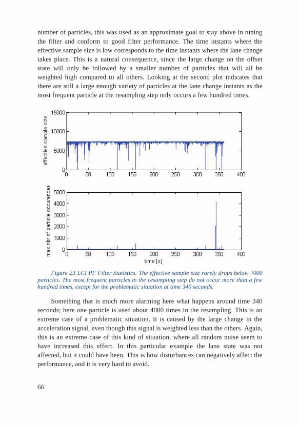
66
number of particles, this was used as an approximate goal to stay above in tuning the filter and conform to good filter performance. The time instants where the effective sample size is low corresponds to the time instants where the lane change takes place. This is a natural consequence, since the large change on the offset state will only be followed by a smaller number of particles that will all be weighted high compared to all others. Looking at the second plot indicates that there are still a large enough variety of particles at the lane change instants as the most frequent particle at the resampling step only occurs a few hundred times.
Figure 23 LCI PF Filter Statistics. The effective sample size rarely drops below 7000 particles. The most frequent particles in the resampling step do not occur more than a few hundred times, except for the problematic situation at time 340 seconds.
Something that is much more alarming here what happens around time 340 seconds; here one particle is used about 4000 times in the resampling. This is an extreme case of a problematic situation. It is caused by the large change in the acceleration signal, even though this signal is weighted less than the others. Again, this is an extreme case of this kind of situation, where all random noise seem to have increased this effect. In this particular example the lane state was not affected, but it could have been. This is how disturbances can negatively affect the performance, and it is very hard to avoid.

67
The next figure, see Figure 24 below, visualizes the changes on the lane state, and more or less indicates that the filter tuning is good as these changes are very clear.
Figure 24 LCI PF Particle Statistics. The changes and direction of change is clearly indicated by the filter, hinting that the tuning of the filter is good.
Even though the changes are clear, it is only a minority of the particles that are affected. This is maybe the clearest motivation for resetting the particles, while keeping the number of particles affected on this quite low level, these signals very clearly indicate the change and there is little room for misinterpretation of the information.
For the other data sets, only the lane estimate, the road width and the lane offset are presented, as two first also correspond to the filter output used for calculating the final estimate and the last makes it possible to verify the lane estimate.
Problematic Situations The next example is from data set 5, in which there is a road segment where no lane markings are available, approximately from time 130 to 140 seconds. This

68
comes from new asphalt on this particular lane, where no new marking have been painted yet. The estimate overview can be seen in Figure 25 below.
Figure 25 LCI PF Estimate Overview - Data Set 5. The time period 130-140 seconds has very poor camera signals because there are no lane markings during this period. This causes the filter to wrongly identify a lane change at the end of this period.
The camera can, during this unmarked section, find some markings, possibly from the next lanes further out, which are identified with reasonably high quality. This confuses the lane estimate, which first shows a hint of indicating a lane change left, but not enough to reset the particles. Instead, in the end of the unmarked section, a lane change to the right is wrongly identified. This kind of situation is hard to compensate for by this filter.
Another situation where a lane change is identified when it should not be is in data set 4. In this data set a small number of camera signals with seeming low quality are confusing the lane estimate at time 310 seconds, causing it to find a lane change where there is none.

69
Figure 26 LCI PF Estimate Overview – Data Set 4. A small number of low quality camera signals are here used to update the filter at time 310 seconds. This wrongly makes the filter identify a lane change.
Why this data is labelled with a higher quality than it should have is hard to know. There are some other indications of low quality data, which does not allow the filter to update. Identifying signals with a higher quality label than they should have is not something that has been implemented.
For all of these data sets the filter correctly identifies all lane changes. In some cases there are disturbances that causes the filter to mistakenly identify additional lane changes.
6.2 Road Edge Detection The implemented IKF for detecting and estimating the distances to the road edges performs well. Compared to the LCI, here the output estimates from the RED have a less stable look to them, much because the input data here is much more complicated to handle.
Figure 27 below shows the filter estimates from data set 8, the same example as used in the previous section.

70
Figure 27 RED IKF Estimate Overview - Data Set 8. This plot shows the distances to the road edges left and right. It is quite clear when lane changes occur, this causes both estimates to change stepwise in the positive or negative direction. There are a total of five lane changes in the plot above; at 20, 120, 160, 320 and 350 seconds respectively.
This shows the estimated distances to the road edges left and right, the last few data points indicating 0 is because of some length differences in the input signals. Knowing that this data shows the same data set as previously seen, one can guess where lane changes occur also from looking at the plot above.
Looking at the lower plot and the distance to the right edge of the road, one can see some indications of the entrances and exits on this side of the road. The clear example is from time 170 to 200, where a small exit is followed by a small entrance. The estimate finds its way back to the actual road edge and the position of the guard rail between the exit and entrance even though they are very close to each other.
There are some large variations in the top plot, this is due to the low number of available measurements for some periods of time, see Figure 28 below. This is typical since normally the vehicle travels on the right side of the road in the slower lanes, and both distance to the left guard rail and other vehicles covers the view to some extent. Especially during the time periods between 50 and 100 seconds and
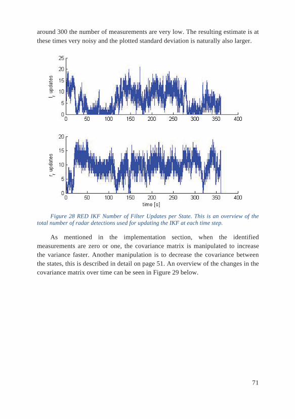
71
around 300 the number of measurements are very low. The resulting estimate is at these times very noisy and the plotted standard deviation is naturally also larger.
Figure 28 RED IKF Number of Filter Updates per State. This is an overview of the total number of radar detections used for updating the IKF at each time step.
As mentioned in the implementation section, when the identified measurements are zero or one, the covariance matrix is manipulated to increase the variance faster. Another manipulation is to decrease the covariance between the states, this is described in detail on page 51. An overview of the changes in the covariance matrix over time can be seen in Figure 29 below.

72
Figure 29 RED IKF Covariance Matrix. This shows the changes in the covariance matrix over time. The high peaks on the variance diagonal come from manipulation; if the detected number of measurements is low the variance is increased by a factor.
The large increases in the state variances occurs at the times where the measurements are low. The covariance is not set to zero, but smaller than the variance terms at all times. The levels of the manipulation of the covariance matrix was determined empirically with simulations on all data sets.
For all data sets these plots have similar characteristics. The assumption made about the road being straight does not seem to have
negatively affected the results, as there are curved sections in all of the used data sets, which cannot be noticed in these plots.
Problematic Situations Large exits and entrances disturb the estimate and will make it hard to find the guard rail in between, instead estimating a very large distance to the right road edge for this time. Even the attempts of manually increasing the variance to better be able to handle these situations have not been able to successfully compensate for this undesired behavior in all cases. An example of this can be seen below in Figure 30.

73
Figure 30 RED IKF Estimate Overview - Data Set 2. Simultaneous changes on the two estimates indicate a lane change at time 20 and 50 seconds. At time 70 second very few detections seem to be found on the left side of the road, causing a fast increase of the standard deviation. At time 170 seconds a medium sized exit on the right side of the road is passed, but the estimate finds its way back to the guard rail after passing. At time 280 a larger exit is passed, this time the estimate does not find the actual guard rail until the entrance brings back the estimate with an entering guard rail at time 330 seconds.
The large exit and following entrance leading back the estimate can be seen at time 280 and 330, between which the distance to the right road edge is around 5 meters rather than the 15 indicated above. Looking instead at time 180 seconds, a smaller, but still quite large exit can be noted. However, here the estimate can in this case find its way back to the actual value.
The top part of Figure 30, showing the distance to the left road edge, also has a noticeable trait. At time 70 seconds the standard deviation increases rapidly over a very short time, this is because very few radar measurements are found to update the filter with during this time.

74
6.3 Lane Association The first step to get the final lane estimate is to calculate the absolute position on the road. There are different time scales on the filter output, because the camera and radar have different measurement frequencies. For this purpose, the values are simply linear interpolated to make the different values comparable at every time, both are scaled to the higher frequency.
The offset parameter is found to be slightly too large if calculated the proposed way, this value is decreased by half to shift the absolute lane estimate closer to the expected values.
Continuing on the previous sections, the data set 8 is the base for the following figures. Firstly, Figure 31 shows the absolute position on the road. With the mentioned tweak on the offset, the figure shows that the position matches the lane numbers on the y-axis well.
Figure 31 Absolut Position on Road - Data Set 8. The calculated absolute lane estimate in blue and the standard deviation in red. Also the Savitzky-Golay filtered signal in cyan and the lagging moving average signal in magenta are plotted. The signal gives the expected value, except for the first 20 seconds where the indication for lane index 1 is not clearly indicated.
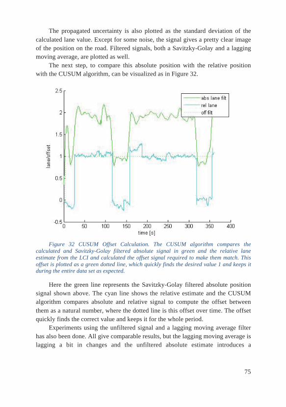
75
The propagated uncertainty is also plotted as the standard deviation of the calculated lane value. Except for some noise, the signal gives a pretty clear image of the position on the road. Filtered signals, both a Savitzky-Golay and a lagging moving average, are plotted as well.
The next step, to compare this absolute position with the relative position with the CUSUM algorithm, can be visualized as in Figure 32.
Figure 32 CUSUM Offset Calculation. The CUSUM algorithm compares the calculated and Savitzky-Golay filtered absolute signal in green and the relative lane estimate from the LCI and calculated the offset signal required to make them match. This offset is plotted as a green dotted line, which quickly finds the desired value 1 and keeps it during the entire data set as expected.
Here the green line represents the Savitzky-Golay filtered absolute position signal shown above. The cyan line shows the relative estimate and the CUSUM algorithm compares absolute and relative signal to compute the offset between them as a natural number, where the dotted line is this offset over time. The offset quickly finds the correct value and keeps it for the whole period.
Experiments using the unfiltered signal and a lagging moving average filter has also been done. All give comparable results, but the lagging moving average is lagging a bit in changes and the unfiltered absolute estimate introduces a

76
disturbance that is affecting the offset calculated from it. The Savitzky-Golay filtered signal is the most stable, and is therefore the one selected to be visualized.
Adding the offset to the relative signal and comparing to the alternative where the absolute signal and the relative signal plus offset signal are weighted together, the result can be seen in Figure 33 below.
Figure 33 Final Lane Estimate – Data Set 8. The red line shows the LCI lane estimate with the added CUSUM offset, it closely follows the expected value. The blue line is a weighted combination, see Equation 1, of the red signal and the previously calculated absolute lane estimate, and the cyan dotted line is the standard deviation of the weighted value.
Both alternatives give very similar and correct results in this case where there are no errors made. However, the weighted versions are approximating the lane estimate from the particle filter as a Gaussian and thereby dropping some of the information.
The CUSUM can compensate for the rare mistakes made in the LCI, such as in data set 4 illustrated in Figure 26. The final estimate will still be reliable after a short period of adjustment, see Figure 34 below, as the CUSUM algorithm notices the large and unexpected deviation between the two positional estimates and compensates for it.

77
Figure 34 Final Lane Estimate – Data Set 4. The actual lane is during this entire data set indexed 1. At time 310 seconds the LCI mistakenly identifies a lane change, which is compensated for by the CUSUM within 10 seconds.
The adaption to errors is fast, it takes less than 10 seconds to again output the correct value after the LCI mistake.
Another data set that is interesting to look at is data set 2, where there was a problematic situation for the road edge detection at a large exit, see Figure 30. Looking at the final lane estimate in Figure 35, it can be concluded that the estimate is not disturbed by the problematic situation.

78
Figure 35 Final Lane Estimate – Data Set 2. After some initial adjustment, the correct lane is correctly identified, even during the time around 300 seconds where the RED has some problems correctly finding the right road edge because of a large exit.
In the example above, it takes the estimate slightly more than 10 seconds to find the correct value, which is 2 until the lane change left at time 20 seconds. This is one of the slower examples, but is still considered acceptable, given that as a part of a future application this would be used in a real-time application and with no reason to restart regularly.
Another problematic situation is a road segment where no lane markings are available, such as a part of data set 5, mentioned earlier and LCI estimated plotted in Figure 25. This mistake is also successfully compensated for, the final lane estimate is shown in

79
Figure 36 Final Lane Estimate – Data Set 5. The expected output of indicating lane 2 is interrupted by a camera disturbance at about 140 seconds, it is compensated for by the CUSUM algorithm within 10 seconds.
The disturbance from the camera is introduced at 140 seconds, after which the lane estimate is corrected by the CUSUM after about 10 seconds.
For most part, the final estimate is very reliable, and is able to compensate for errors made by the LCI or the RED.
6.4 Final Performance This is absolutely a feasible strategy extracting the information about in which lane the vehicle is currently driving. It is quite computationally heavy itself, and as the implementation focus has been on results rather than achieving a fast, light-weight method of getting to this result, there is room for plenty of improvement here. For example, the radar detections are stored in the source data mat-files with their numbered id in the name. These data fields are read in MATLAB with an extremely time-consuming combination of string formatting and variable name generating from the formed strings. This kind of handling in the data severely increases the total runtime.

80
Knowing the current implementation has not focused on speed at all, some reference values for will be mentioned, but these should not be given too much attention. The total time from reading in the values from the mat-files to plotting the final lane estimate is approximately 190 seconds on a reasonably fast computer. Of this time, 120 seconds are spent by the particle filter, and 60 seconds by the iterated Kalman filter where the mentioned unreasonably complicated reading of data takes place. This gives an indication of the internal ratios of the time spent.

81
7. Discussion The overall result is good, the possibilities of performing a lane association with this method has been explored and results of high quality are found.
This setup can with high precision extract the specified information from the supplied data. Some problematic situations are encountered, which are not optimally handled along the way, but still do not affect the results for more than short isolated periods of time. Even though these problematic situations have received quite a lot of attention in the report for discussing weaknesses in the implementation, they are quite rare in the large number of simulations that have been performed in total.
All MATLAB implementations have been done from a very low level to have full freedom to manipulate and tweak all parts of the implementation for as good performance as possible.
This approach of solving the given problem has to some extent ideas in common with the literature mentioned in chapter 2. Compared to what is presented there, this implementation is fairly simple. The information is not used in quite the same way, and this approach is somewhat more straight-forward. The outcome here is still good results, but this is just one of many different ways of solving the problem, and possibly many of the others are better or more efficient.
7.1 Model CritiqueAll models are simplifications of the real world, but the ones used in this project seem to be scraped down to the bare essentials. Completely ignoring longitudinal movement intuitively feels strange considering that for a truck, longitudinal movement is one of the first associations one make. Even these simplifications seem to fulfill the purpose in most cases. Also, looking at the distances to the road edges only as constants seems to be too simple.

82
The complete problem is very complex, and this is considered a reasonable first step. Since the output closely resembles the expected lane index it is hard to motivate a more complex model at this very early stage of development, where exploring possibilities was the focus.
Another aspect, related to the final lane association part as an example, is the general discussion about what data is given the most importance. Here the calculated absolute position on the road is mostly relying on radar detections on the left side of the road, as the offset is calculated from this side. The distance to the right side of the road is only used, together with the distance to the left, to calculate the total road width. Still, it is generally easier to detect right side of the road, because of the positioning is more often close to the right side of the road giving more detections from this side of the road. However, the left side distance is generally more stable, with no exits or entrances disturbing the estimate. Possibly this kind of arguments could have been given more attention in the development.
7.2 Filter Critique The main functionality of the filters has been determined to be good in general, but there are some problems that has been pointed out in the results section. There is also some general thoughts that will be presented below, per filter.
It should also be mentioned that the other filters mentioned on page 26 could be used in different combinations, not all alternatives with this filtering approach has been investigated. One could also consider some kind of machine learning approach, considering the large amounts of data available, but this is outside the scope of this project.
Particle Filter There is some critique in [33] on using PFs on systems of high dimensionality and highly dynamic states, such as accelerations and unmeasured velocities. High dimensionality is not clearly defined, but can be interpreted as more than three, where six definitely is high dimensionality. The main issue is that the particle representation would be too sparse to represent the posterior distribution in a meaningful way. This application could be a typical example where the performance is at risk, but the relatively large number of particles seems to compensate for this and the filter obviously produces meaningful output.

83
As been shown in the results section, the implemented filter heavily relies on the high quality of the camera signal. It will be prone to make mistakes if the signal does not reach the expected quality, but this is rare in the data used during the development. Fortunately, if an error occurs, it will be compensated for later on and will not be affecting the final lane estimate for more than a short time.
There is a restriction on the filter update, which is completely skipped if the camera signals for the particular time step is if too low quality, only noise will be added in this case. This is realized to be naïve, but it works for all data sets that has been used during development. Most certainly there are data sets where this is a too strong simplification, it will probably be most sensitive to this kind of disturbance when it occurs at the same time as a lane change.
Iterated Kalman Filter The IKF is, according to theory, sensitive to deviations in the model and noise covariance matrix to the real situation. The implemented filter seems to perform well, even with the very simplified model and the ad-hoc chosen noise covariance.
The problem is, however, for the filter to find its way back to the correct estimate after large exits. Even though this problem is not affecting the final lane estimate, this is undesired behavior by the filter. A more sophisticated model or a different approach to the problem may handle this kind of problem better.
7.3 Data Selection Since the development has been tightly intertwined with available data, the data itself and the selection process will be elaborated further in a critical manner. The selection of data was made by looking at the logged video files, in a completely unstructured manner. A data set was considered interesting if it was recorded completely on a highway, and preferably contained one or more situations including lane changes, exits of varying sizes or other challenges for the filters.
Some sets were further discarded when some of the used data had not been logged at that particular time for some reason. Large amounts of logged data was available, the actual selection process was quite random.
A wider range of data could be interesting to look at in the future, even though, within the case of highway scenarios, a large variation of situations has been examined.

84
7.4 Structure of Computations The structure and manner in which the calculations are carried out is also worth mentioning. The final structure in Figure 7 was something that evolved over time, and was not set from the beginning.
It has been considered to be of importance that data is only used once, and no information is being reused in a way that could cause loops, increasing importance of faulty assumptions which might compromise the ability of the filters. The small exception is that both the lane width and the LCI lane estimate both are based on the same camera data to some extent, and these are later merged in the final step of the lane association, LA. The total number of lanes from the map data is more or less considered an at all times perfect constant in this case.
7.5 Computational Complexity This implementation is rather computationally heavy, and is in its current form not suitable for use in a vehicle. Even though the purpose here is to investigate possibilities and methods, some thought should be put to this practical issue for potential future implementations. The most resource demanding part is the particle filter.
There are examples of implementations of particle filters in embedded systems in literature, where different variants making the filter better suited for the limited environment an embedded system provides compared to a desktop computer. As an example, there is a variant called a mean shift embedded particle filter used for visual pattern recognition, which claims to reduce the number of required particles with 85 % [45]. Other examples are [46], [47] and [48], where a hardware-close implementations are suggested.
It is considered that there are good possibilities to implement particle filters, also for this application, in embedded systems given the research on the area.
7.6 Conclusion Essentially, this project shows that the data chosen as input here can easily be used to extract information about which lane a vehicle is currently driving in. The implemented filters and algorithms does the job, but are computationally heavy and there is room for improvement here.

85
Knowing the current lane index is not in itself revolutionary in any way, but for future applications it could be an important component.
7.7 Future Research This project opens for many future possibilities. A first experiment could be adapting the current implementation for real-time use and test it in a real truck.
As mentioned earlier in this chapter, looking at more advanced models could give opportunities of predicting lane indices and lane changes further ahead in time. One example is the current assumption that the road in front of the vehicle is straight, this in combination with looking at the movement on the road in a more complex way could open for the prediction further ahead in time.
Another possibility is looking at data in a more clever way. For example, to look at guard rail detection as an object instead of individual detections which can be assumed to be a guard rail. This could increase the understanding for when an exit is coming up or other problematic situations.
Looking at a wider range of situations could also be an interesting future extension. Other situations than highways, where maybe the availability of guard rails are not as certain, poses other difficulties,
The two filters could, with some benefits, exchange more information, giving the final estimate in a one step process possibly. It could be of interest to look at possibilities on implementing one larger, maybe a marginalized particle filter, instead of the two smaller ones, directly sharing and using the information extracted. This could increase the complexity and the benefits with modularization would be lost.
As the purpose of this project is to extract information about lane association to make it possible for other future systems and applications necessary for automated driving to function, these should be the main priority in the future. It must be further investigated whether or not the extracted information is of high enough quality for these systems, but at this point this is difficult. In any case, this is one step in the right direction.

86
8. References
[1] European Commission, "Towards a strategy to address CO2 emissions from Heavy-Duty Vehicles," 31 October 2013. [Online]. Available: http://ec.europa.eu/clima/policies/transport/vehicles/heavy/index_en.htm.[Accessed 1 January 2014].
[2] Scania, "Scania i korthet 2012/2013," Kreab Gavin Andersson, Trosa, 2013.
[3] Wikipedia, "Platoon (automobile)," Wikimedia Foundation, Inc., 26 November 2013. [Online]. Available: http://en.wikipedia.org/wiki/Platoon_(automobile). [Accessed 1 January 2014].
[4] Trafiksäkerhetsverket, "Nollvisionen," 28 August 2012. [Online]. Available: http://www.trafikverket.se/Privat/Trafiksakerhet/Vart-trafiksakerhetsarbete/Trafiksakerhetsmal/Nollvisionen/. [Accessed 29 December 2013].
[5] Transportstyrelsen, "Historik Färdsätt," [Online]. Available: http://www.transportstyrelsen.se/sv/Press/Statistik/Vag/Olycksstatistik/Olycksstatistik-vag/Nationell-statistik1/Arsvis-statistik/Historik-fardsatt/. [Accessed 29 December 2013].
[6] J. Treat, N. Tumbas, S. McDonald, D. Shinar, R. Hume, R. Mayer, R. Stansifer and N. Castellan, "Tri-Level Study of the Causes of Traffic Accidents: Final Report," Institute for Research in Public Safety, 1977.
[7] F. Gustafsson, "Automotive Safety Systems," IEEE Signal Processing Magazine, vol. 26, no. 4, pp. 32-47, 2009.
[8] Wikipedia, "Advanced driver assistance systems," Wikimedia Foundation, Inc., 28 February 2013. [Online]. Available:
87
http://en.wikipedia.org/wiki/Advanced_driver_assistance_systems. [Accessed 1 January 2014].
[9] Scania, "Scania Image Archive," 2013. [Online]. Available: http://www.scania.com/media/imagebank/. [Accessed 8 February 2014].
[10] The MathWorks, Inc., "MATLAB - The Language of Technical Computing - MathWorks Nordic," The MathWorks, Inc., 2014. [Online]. Available: http://www.mathworks.se/products/matlab/. [Accessed 31 January 2014].
[11] A. Assidiq, O. Khalifa, R. Islam and S. Khan, "Real Time Lane Detection for Autonomous Vehicles," in Computer and Communication Engineering, 2008. International Conference on, Kuala Lumpur, 2008.
[12] Wikipedia, "Lane Departure Warning System," WikiMedia Foundation, Inc., 8 January 2014. [Online]. Available: http://en.wikipedia.org/wiki/Lane_departure_warning_system. [Accessed 11 February 2014].
[13] J. Clanton, D. Bevly and A. Hodel, "A Low-Cost Solution for an Integrated Multisensor Lane Departure Warning System," IntelligentTransportation Systems, IEEE Transactions on, vol. 10, no. 1, pp. 47-59, 2009.
[14] C. Adam, R. Schubert, N. Mattern and G. Wanielik, "Probabilistic Road Estimation and Lane Association Using Radar Detection," in Information Fusion (FUSION), 2011 Proceedings of the 14th International Conference on, Chicago, IL, 2011.
[15] G. Alessandretti, A. Broggi and P. Cerri, "Vehicle and Guard Rail Detection Using Radar and Vision Data Fusion," IntelligentTransportation Systems, IEEE Transactions on, vol. 8, no. 1, pp. 95-105, 2007.
[16] H. Loose, U. Franke and C. Stiller, "Kalman Particle Filter for Lane Recognition on Rural Roads," in Intelligent Vehicles Symposium, 2009 IEEE, Xi'an, 2009.
[17] F. Janda, S. Pangerl, E. Lang and E. Fuchs, "Road Boundary Detection for Run-off Road Prevention based on the Fusion of Video and Radar," in Intelligent Vehicles Symposium (IV), 2013 IEEE, Gold Coast, QLD, 2013.
[18] S. Chung and H. Huang, "Relative-Absolute Map Filter for Simultaneous
88
Localization and Mapping," in Intelligent Robots and Systems, 2006 IEEE/RJS International Conference on, Beijing, 2006.
[19] CAN in Automation (CiA), "CAN History," 2013. [Online]. Available: http://www.can-cia.de/index.php?id=161. [Accessed 3 January 2014].
[20] CAN in Automotion (CiA), "CAN Protocol," 2013. [Online]. Available: www.can-cia.de/index.php?id=systemdesign-can-protocol. [Accessed 4 February 2014].
[21] K. Johansson, M. Törngren and L. Nielsen, "Vehicle Application ofController Area Network," in Handbook of Networked and Embedded Control Systems, Basel, Birkhäuser, 2005, pp. 741-765.
[22] Wikipedia, "OSI Model," Wikimedia Foundation, Inc., 2 January 2014. [Online]. Available: http://en.wikipedia.org/wiki/OSI_model. [Accessed 3 January 2014].
[23] T. Nolte, H. Hansson and C. Norström, "Probabilistic Worst-Case Response-Time Analysis for the Controller Area Network," Department of Computer Science and Engineering, Mälardalen University, Västerås, 2003.
[24] International Organization for Standardization, "Search - ISO (11898)," [Online]. Available: http://www.iso.org/iso/search.htm?qt=11898&published=on&active_tab=standards. [Accessed 3 January 2014].
[25] B. Yu and A. Jain, "Lane Boundary Detection Using a Multiresolution Hough Transform," in Proceedings - International Conference on Image Processing, Santa Barbara, CA, 1997.
[26] C. Lundquist, Sensor Fusion for Automotive Applications, Linköping: LiU-Tryck, 2011.
[27] C. Lundquist, U. Orguner and T. Schön, "Tracking Stationary Extended Objects for Road Mapping using Radar Measurements," in IntelligentVehicles Symposium, Xi'an, 2009.
[28] E. Richter, M. Obst, M. Noll and G. Wanielik, "Tracking Multiple Extended Objects - A Markov Chain Monte Carlo Approach," in Information Fusion (FUSION), Chicago, IL, 2011.
[29] Wikipedia, "Sensor Fusion," Wikimedia Foundation, Inc., 14 December 2013. [Online]. Available: http://en.wikipedia.org/wiki/Sensor_fusion. [Accessed 3 January 2014].

89
[30] F. Gustafsson, Statistical Sensor Fusion, Lund: Studentlitteratur, 2012.[31] M. Arulampalam, S. Maskell, N. Gordon and T. Clapp, "A Tutorial on
Particle Filters for Online Nonlinear/Non-Gaussian Bayesian Tracking," IEEE Transactions on Signal Processing, vol. 50, no. 2, pp. 174-188, 2002.
[32] T. Schön, "Solving Nonlinear State Estimation Problems Using Particle Filters - An Engineering Perspective," Department of Automatic Control, Linköping University, Linköping, 2010.
[33] F. Gustafsson, "Particle Filter Theory and Practice with Positioning Applications," IEEE Aerospace and Electronic Systems Magazines, vol.25, no. 7, pp. 53-81, 2010.
[34] D. Alspach and H. Sorenson, "Nonlinear Bayesian Estimation Using Gaussian Sum Approximations," IEEE Transactions on Automatic Control, vol. 17, no. 4, pp. 439-448, 1972.
[35] N. Gordon, D. Salmond and A. Smith, "Novel approach to nonlinear/non-Gaussian Bayesian state estimation," IEE Proceedings on Radar and Signal Processing, vol. 140, no. 2, pp. 107-113, 1993.
[36] E. Orhan, "Particle Filtering," 11 August 2012. [Online]. Available: www.cns.nyu.edu/~eorhan/notes/particle-filtering.pdf. [Accessed 14 January 2014].
[37] R. Douc, O. Cappé and E. Moulines, "Comparison of Resampling Schemes for Particle Filtering," Image and Signal Processing and Analysis, pp. 64-69, 2005.
[38] L. Svensson, "Comments on the Resampling Step in Particle Filtering," 16 March 2012. [Online]. Available: http://pingpong.chalmers.se/public/pp/public_noticeboard_attachment/fetch?messageId=35447&fileId=827809. [Accessed 13 January 2014].
[39] NIST/SEMATECH, "e-Handbook of Statistical Methods, 6.3.2.3 CUSUM Control Charts," 10 October 2013. [Online]. Available: www.itl.nist.gov/div898/handbook/pmc/section3/pmc323.htm. [Accessed 29 January 2014].
[40] Vector Informatik GmbH, "CANalyzer," Vector Informatik GmbH, 24 January 2014. [Online]. Available: http://vector.com/vi_canalyzer_en.html. [Accessed 31 January 2014].
[41] Sektionen Utformning av Vägar och Gator, "Vägar och Gators

90
Utformning - Linjeföring," Vägverket, Borlänge, 2004. [42] Wikipedia, "Propagation of Uncertainity," Wikimedia Foundation, Inc.,
3 December 2013. [Online]. Available: http://en.wikipedia.org/wiki/Propagation_of_uncertainity. [Accessed 30 January 2014].
[43] Wikipedia, "Savitzky-Golay Filter," WikiMedia Foundation, Inc., 21 January 2014. [Online]. Available: http://en.wikipedia.org/wiki/Savitzky-Golay_filter. [Accessed 7 February 2014].
[44] Wikipedia, "Moving Average," WikiMedia Foundation, Inc., 29 January 2014. [Online]. Available: http://en.wikipedia.org/wiki/Moving_average. [Accessed 7 February 2014].
[45] C. Shan, T. Tan and Y. Wei, "Real-Time Hand Tracking using a Mean Shift Embedded Particle Filter," Pattern Recognition, vol. 40, no. 7, pp. 1958-1970, 2007.
[46] G. Li, B. Li, Z. Liu and X. Chen, "Implementation and Optimization ofParticle Filter Tracking Algorithm on Multi-DSPs System," in Cybernetics and Intelligent Systems, 2008 IEEE Conference on,Chengdu, 2008.
[47] S. Saha, N. Bambha and S. Bhattachayya, "Design and Implementation of Embedded Computer Vision Systems Based on Particle Filters," Computer Vision and Image Understanding, vol. 114, no. 11, pp. 1203-1214, 2010.
[48] R. Farah, Q. Gan, J. Langlois and G. Bilodeau, "A Tracking Algorithm Suitable for Embedded Systems Implementation," in Electronics,Circuits and Systems (ICECS), 2011 18th IEEE International Conference on, Beirut, 2011.


Lund UniversityDepartment of Automatic ControlBox 118SE-221 00 Lund Sweden
Document nameMASTER THESISDate of issueFebruary 2014Document NumberISRN LUTFD2/TFRT--5937--SE
Author(s)
Elin DahlinSupervisorPär Degerman, ScaniaBo Bernhardsson, Dept. of Automatic Control, Lund University, Sweden (examiner)Sponsoring organization
Title and subtitle
Probabilistic Lane Association
Abstract
Lane association is the problem of determining in which lane a vehicle is currently driving, which is of interest for automated driving where the vehicle must understand its surroundings. Limited to highway scenarios, a method combining data from different sensors to extract information about the currently associated lane is presented.
The suggested method splits the problem in two main parts, lane change identification and road edge detection. The lane change identification mainly uses information from the camera to model the lateral movement on the road and identifies the lane changes as a relative position on the road. This part is implemented with a particle filter. The road edge detection enters radar detections to an iterated Kalman filter and estimates the distances to the road edges.
Finally, a combination of the filter outputs makes it possible to compute an absolute position on the road. Comparing the relative and absolute positioning then leads to the desired lane association estimate.
The results produced are reliable and encourages to continue approaching this problem in a similar manner, but the current implementation is computationally heavy.
Keywords
Classification system and/or index terms (if any)
Supplementary bibliographical information
ISSN and key title0280-5316
ISBN
LanguageEnglish
Number of pages1-90
Recipient’s notes
Security classification
http://www.control.lth.se/publications/