Probabilistic Data Association for Semantic SLAM

Sean L. Bowman Nikolay Atanasov Kostas Daniilidis George J. Pappas

Abstract— Traditional approaches to simultaneous localiza-tion and mapping (SLAM) rely on low-level geometric featuressuch as points, lines, and planes. They are unable to assignsemantic labels to landmarks observed in the environment.Furthermore, loop closure recognition based on low-level fea-tures is often viewpoint-dependent and subject to failure inambiguous or repetitive environments. On the other hand,object recognition methods can infer landmark classes andscales, resulting in a small set of easily recognizable landmarks,ideal for view-independent unambiguous loop closure. In amap with several objects of the same class, however, a crucialdata association problem exists. While data association andrecognition are discrete problems usually solved using discreteinference, classical SLAM is a continuous optimization overmetric information. In this paper, we formulate an optimizationproblem over sensor states and semantic landmark positionsthat integrates metric information, semantic information, anddata associations, and decompose it into two interconnectedproblems: an estimation of discrete data association and land-mark class probabilities, and a continuous optimization over themetric states. The estimated landmark and robot poses affectthe association and class distributions, which in turn affectthe robot-landmark pose optimization. The performance of ouralgorithm is demonstrated on indoor and outdoor datasets.

I. INTRODUCTION

In robotics, simultaneous localization and mapping (SLAM)is the problem of mapping an unknown environment whileestimating a robot’s pose within it. Reliable navigation, objectmanipulation, autonomous surveillance, and many other tasksrequire accurate knowledge of the robot’s pose and thesurrounding environment. Traditional approaches to SLAMrely on low-level geometric features such as corners [1],lines [2], and surface patches [3] to reconstruct the metric3-D structure of a scene but are mostly unable to infersemantic content. On the other hand, recent methods forobject recognition [4]–[6] can be combined with approximate3D reconstruction of the environmental layout from singleframes using priors [7], [8]. These are rather qualitative single3D snapshots rather than the more precise mapping we needfor a robot to navigate. The goal of this paper is to address themetric and semantic SLAM problems jointly, taking advantageof object recognition to tightly integrate both metric andsemantic information into the sensor state and map estimation.In addition to providing a meaningful interpretation of thescene, semantically-labeled landmarks address two criticalissues of geometric SLAM: data association (matching sensorobservations to map landmarks) and loop closure (recognizingpreviously-visited locations).

The authors are with GRASP Lab, University of Pennsylvania,Philadelphia, PA 19104, USA, {seanbow, atanasov, kostas,pappasg}@seas.upenn.edu.

We gratefully acknowledge support by TerraSwarm, one of six centersof STARnet, a Semiconductor Research Corporation program sponsored byMARCO and DARPA and the following grants: ARL MAST-CTA W911NF-08-2-0004, ARL RCTA W911NF-10-2-0016.

Approaches to SLAM were initially most often basedon filtering methods in which only the most recent robotpose is estimated [9]. This approach is in general verycomputationally efficient, however because of the inabilityto estimate past poses and relinearize previous measurementfunctions, errors can compound [1]. More recently, batchmethods that optimize over entire trajectories have gainedpopularity. Successful batch methods typically representoptimization variables as a set of nodes in a graph (a “posegraph”). Two robot-pose nodes share an edge if an odometrymeasurement is available between them, while a landmarkand a robot-pose node share an edge if the landmark wasobserved from the corresponding robot pose. This pose graphoptimization formulation of SLAM traces back to Lu andMilios [10]. In recent years, the state of the art [11], [12]consists of iterative optimization methods (e.g., nonlinearleast squares via the Gauss-Newton algorithm) that achieveexcellent performance but depend heavily on linearizationof the sensing and motion models. This becomes a problemwhen we consider including discrete observations, such asdetected object classes, in the sensing model.

One of the first systems that used both spatial and semanticrepresentations was proposed by Galindo et al. [13]. A spatialhierarchy contained camera images, local metric maps, and theenvironment topology, while a semantic hierarchy representedconcepts and relations, which allowed room categories to beinferred based on object detections. Many other approaches[14]–[19] extract both metric and semantic information buttypically the two processes are carried out separately andthe results are merged afterwards. The lack of integrationbetween the metric and the semantic mapping does not allowthe object detection confidence to influence the performanceof the metric optimization. Focusing on the localizationproblem only, Atanasov et al. [20] incorporated semanticobservations in the metric optimization via a set-based Bayesfilter. The works that are closest to ours [21]–[24] considerboth localization and mapping and carry out metric andsemantic mapping jointly. SLAM++ [22] focuses on a real-time implementation of joint 3-D object recognition and RGB-D SLAM via pose graph optimization. A global optimizationfor 3D reconstruction and semantic parsing has been proposedby [25], which is the closest work in semantic/geometric jointoptmization. The main difference is that 3D space is voxelizedand landmarks and/or semantic labels are assigned to voxelswhich are connected in a conditional random field whileour approach allows the estimation of continuous pose ofobjects. Bao et al. [21] incorporate camera parameters, objectgeometry, and object classes into a structure from motionproblem, resulting in a detailed and accurate but large andexpensive optimization. A recent comprehensive survey ofsemantic mapping can be found in [26].

2017 IEEE International Conference on Robotics and Automation (ICRA)Singapore, May 29 - June 3, 2017

978-1-5090-4632-4/17/$31.00 ©2017 IEEE 1722

Most related work uses a somewhat arbitrary decompositionbetween data association, pose graph optimization, and objectrecognition. Our work makes the following contributions tothe state of the art:• our approach is the first to tightly couple inertial,

geometric, and semantic observations into a singleoptimization framework,

• we provide a formal decomposition of the joint metric-semantic SLAM problem into continuous (pose) anddiscrete (data association and semantic label) optimiza-tion sub-problems,

• we carry out experiments on several long-trajectory realindoor and outdoor datasets, which include odometryand visual measurements in cluttered scenes and varyinglighting conditions.

II. PROBABILISTIC DATA ASSOCIATION IN SLAM

Consider the classical localization and mapping problem,in which a mobile sensor moves through an unknownenvironment, modeled as a collection L , {`m}Mm=1 ofM static landmarks. Given a set of sensor measurementsZ , {zk}Kk=1, the task is to estimate the landmark positionsL and a sequence of poses X , {xt}Tt=1 representing thesensor trajectory. Most existing work focuses on estimatingX and L and rarely emphasizes that the data associationD , {(αk, βk)}Kk=1 stipulating that measurement zk oflandmark `βk

was obtained from sensor state xαkis in

fact unknown. A complete statement of the SLAM probleminvolves maximum likelihood estimation of X , L, and Dgiven the measurements Z:

X , L, D = argmaxX ,L,D

log p(Z|X ,L,D) (1)

The most common approach to this maximization has beento decompose it into two separate estimation problems. First,given prior estimates X 0 and L0, the maximum likelihoodestimate D of the data association D is computed (e.g., viajoint compatability branch and bound [27] or the Hungarianalgorithm [28]). Then, given D, the most likely landmarkand sensor states are estimated1:

D = argmaxD

p(D|X 0,L0,Z) (2a)

X , L = argmaxX ,L

log p(Z|X ,L, D) (2b)

The second optimization above is typically carried out viafiltering [30]–[32] or pose-graph optimization [11], [12].

The above process has the disadvantage that an incorrectlychosen data association may have a highly detrimental effecton the estimation performance. Moreover, if ambiguousmeasurements are discarded to avoid incorrect associationchoices, they will never be reconsidered later when refinedestimates of the sensor pose (and hence their data association)are available. Instead of a simple one step process, then, it ispossible to perform coordinate descent, which iterates the

1Note that the first maximization in (2a) assumes that p(D|X 0,L0) isuniform. This is true when there are no false positive measurements ormissed detections. A more sophisticated model can be obtained using ideasfrom [29].

two maximization steps as follows:

Di+1 = argmaxD

p(D|X i,Li,Z) (3a)

X i+1,Li+1 = argmaxX ,L

log p(Z|X ,L,Di+1) (3b)

This resolves the problem of being able to revisit associationdecisions once state estimates improve but does little toresolve the problem with ambiguous measurements sincea hard decision on data associations is still required. Toaddress this, rather than simply selecting D as the mode ofp(D|X ,L,Z), we should consider the entire density of Dwhen estimating X and L. Given initial estimates X i, Li,an improved estimate that utilizes the whole density of Dcan be computed by maximizing the expected measurementlikelihood via expectation maximization (EM):

X i+1,Li+1=argmaxX ,L

ED[log p(Z|X ,L,D) | X i,Li,Z

](4)

=argmaxX ,L

∑D∈D

p(D|X i,Li,Z) log p(Z|X ,L,D)

where D is the space of all possible values of D. This EMformulation has the advantage that no hard decisions on dataassociation are required since it “averages” over all possibleassociations. To compare this with the coordinate descentformulation in (3), we can rewrite (4) as follows:

argmaxX ,L

∑D∈D

K∑k=1

p(D|X i,Li,Z) log p(zk|xαk, `βk

)

= argmaxX ,L

K∑k=1

M∑j=1

wikj log p(zk|xαk, `j) (5)

where wikj ,∑D∈D(k,j) p(D|X i,Li,Z) is a weight, in-

dependent of the optimization variables X and L, thatquantifies the influence of the “soft” data association, andD(k, j) , {D ∈ D | βk = j} ⊆ D is the set of all dataassociations such that measurement k is assigned to landmarkj. Note that the coordinate descent optimization (3b) has asimilar form to (5), except that for each k there is exactlyone j such that wikj = 1 and wikl = 0 for all l 6= j.

We can also show that the EM formulation, besides beinga generalization of coordinate descent, is equivalent to thefollowing matrix permanent maximization problem.

Proposition 1. If p(D | X i,Li) is uniform, the maximizersof the EM formulation in (4) and the optimization below areequal:

X i+1,Li+1 = argmaxX ,L

per(Qi(X ,L)),

where per denotes the matrix permanent2, Qi(X ,L) is amatrix with elements

[Qi]kj

:= p(zk|xij , `ij)p(zk|xj , `j) and{(xij , `ij)} and {(xj , `j)} are enumerations of the sets X i×Liand X × L, respectively.

Proof. See Appendix I.

Similar to the coordinate descent formulation, the EM for-

2The permanent of an n × m matrix A = [A(i, j)] with n ≤ m isdefined as per(A) :=

∑π

∏ni=1 A(i, π(i)), where the sum is over all

one-to-one functions π : {1, . . . , n} → {1, . . . ,m}.

1723

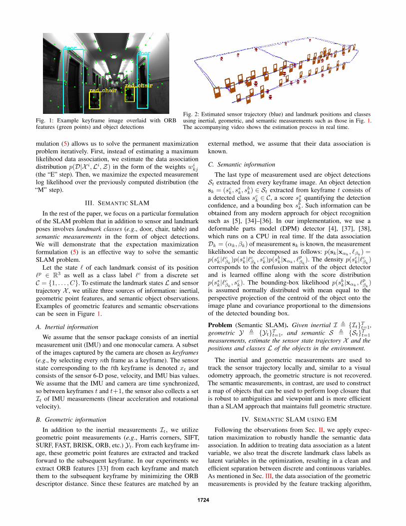
Fig. 1: Example keyframe image overlaid with ORBfeatures (green points) and object detections

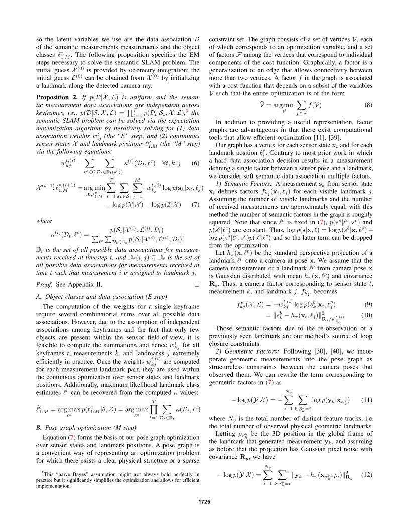
Fig. 2: Estimated sensor trajectory (blue) and landmark positions and classesusing inertial, geometric, and semantic measurements such as those in Fig. 1.The accompanying video shows the estimation process in real time.

mulation (5) allows us to solve the permanent maximizationproblem iteratively. First, instead of estimating a maximumlikelihood data association, we estimate the data associationdistribution p(D|X i,Li,Z) in the form of the weights wikj(the “E” step). Then, we maximize the expected measurementlog likelihood over the previously computed distribution (the“M” step).

III. SEMANTIC SLAM

In the rest of the paper, we focus on a particular formulationof the SLAM problem that in addition to sensor and landmarkposes involves landmark classes (e.g., door, chair, table) andsemantic measurements in the form of object detections.We will demonstrate that the expectation maximizationformulation (5) is an effective way to solve the semanticSLAM problem.

Let the state ` of each landmark consist of its position`p ∈ R3 as well as a class label `c from a discrete setC = {1, . . . , C}. To estimate the landmark states L and sensortrajectory X , we utilize three sources of information: inertial,geometric point features, and semantic object observations.Examples of geometric features and semantic observationscan be seen in Figure 1.

A. Inertial information

We assume that the sensor package consists of an inertialmeasurement unit (IMU) and one monocular camera. A subsetof the images captured by the camera are chosen as keyframes(e.g., by selecting every nth frame as a keyframe). The sensorstate corresponding to the tth keyframe is denoted xt andconsists of the sensor 6-D pose, velocity, and IMU bias values.We assume that the IMU and camera are time synchronized,so between keyframes t and t+1, the sensor also collects a setIt of IMU measurements (linear acceleration and rotationalvelocity).

B. Geometric information

In addition to the inertial measurements It, we utilizegeometric point measurements (e.g., Harris corners, SIFT,SURF, FAST, BRISK, ORB, etc.) Yt. From each keyframe im-age, these geometric point features are extracted and trackedforward to the subsequent keyframe. In our experiments weextract ORB features [33] from each keyframe and matchthem to the subsequent keyframe by minimizing the ORBdescriptor distance. Since these features are matched by an

external method, we assume that their data association isknown.

C. Semantic information

The last type of measurement used are object detectionsSt extracted from every keyframe image. An object detectionsk = (sck, s

sk, s

bk) ∈ St extracted from keyframe t consists of

a detected class sck ∈ C, a score ssk quantifying the detectionconfidence, and a bounding box sbk. Such information can beobtained from any modern approach for object recognitionsuch as [5], [34]–[36]. In our implementation, we use adeformable parts model (DPM) detector [4], [37], [38],which runs on a CPU in real time. If the data associationDk = (αk, βk) of measurement sk is known, the measurementlikelihood can be decomposed as follows: p(sk|xαk

, `βk) =

p(sck|`cβk)p(ssk|`cβk

, sck)p(sbk|xαk

, `pβk). The density p(sck|`cβk

)corresponds to the confusion matrix of the object detectorand is learned offline along with the score distributionp(ssk|`cβk

, sck). The bounding-box likelihood p(sbk|xαk, `pβk

)is assumed normally distributed with mean equal to theperspective projection of the centroid of the object onto theimage plane and covariance proportional to the dimensionsof the detected bounding box.

Problem (Semantic SLAM). Given inertial I , {It}Tt=1,geometric Y , {Yt}Tt=1, and semantic S , {St}Tt=1

measurements, estimate the sensor state trajectory X and thepositions and classes L of the objects in the environment.

The inertial and geometric measurements are used totrack the sensor trajectory locally and, similar to a visualodometry approach, the geometric structure is not recovered.The semantic measurements, in contrast, are used to constructa map of objects that can be used to perform loop closure thatis robust to ambiguities and viewpoint and is more efficientthan a SLAM approach that maintains full geometric structure.

IV. SEMANTIC SLAM USING EM

Following the observations from Sec. II, we apply expec-tation maximization to robustly handle the semantic dataassociation. In addition to treating data association as a latentvariable, we also treat the discrete landmark class labels aslatent variables in the optimization, resulting in a clean andefficient separation between discrete and continuous variables.As mentioned in Sec. III, the data association of the geometricmeasurements is provided by the feature tracking algorithm,

1724

so the latent variables we use are the data association Dof the semantic measurements measurements and the objectclasses `c1:M . The following proposition specifies the EMsteps necessary to solve the semantic SLAM problem. Theinitial guess X (0) is provided by odometry integration; theinitial guess L(0) can be obtained from X (0) by initializinga landmark along the detected camera ray.

Proposition 2. If p(D|X ,L) is uniform and the seman-tic measurement data associations are independent acrosskeyframes, i.e., p(D|S,X ,L) =

∏Tt=1 p(Dt|St,X ,L),3 the

semantic SLAM problem can be solved via the expectationmaximization algorithm by iteratively solving for (1) dataassociation weights wtij (the “E” step) and (2) continuoussensor states X and landmark positions `p1:M (the “M” step)via the following equations:

wt,(i)kj =

∑`c∈C

∑Dt∈Dt(k,j)

κ(i)(Dt, `c) ∀t, k, j (6)

X (i+1), `p,(i+1)1:M =argmin

X ,`p1:M

T∑t=1

∑sk∈St

M∑j=1

−wt,(i)kj log p(sk|xt, `j)

− log p(Y|X )− log p(I|X ) (7)

where

κ(i)(Dt, `c) =p(St|X (i),L(i),Dt)∑

`c∑Dt∈Dt

p(St|X (i),L(i),Dt),

Dt is the set of all possible data associations for measure-ments received at timestep t, and Dt(i, j) ⊆ Dt is the set ofall possible data associations for measurements received attime t such that measurement i is assigned to landmark j.

Proof. See Appendix II.

A. Object classes and data association (E step)The computation of the weights for a single keyframe

require several combinatorial sums over all possible dataassociations. However, due to the assumption of independentassociations among keyframes and the fact that only fewobjects are present within the sensor field-of-view, it isfeasible to compute the summations and hence wtkj for allkeyframes t, measurements k, and landmarks j extremelyefficiently in practice. Once the weights wt,(i)kj are computedfor each measurement-landmark pair, they are used withinthe continuous optimization over sensor states and landmarkpositions. Additionally, maximum likelihood landmark classestimates `c can be recovered from the computed κ values:

ˆc1:M = argmax

`cp(`c1:M |θ,Z) = argmax

`c

T∏t=1

∑Dt∈Dt

κ(Dt, `c)

B. Pose graph optimization (M step)Equation (7) forms the basis of our pose graph optimization

over sensor states and landmark positions. A pose graph isa convenient way of representing an optimization problemfor which there exists a clear physical structure or a sparse

3This “naıve Bayes” assumption might not always hold perfectly inpractice but it significantly simplifies the optimization and allows for efficientimplementation.

constraint set. The graph consists of a set of vertices V , eachof which corresponds to an optimization variable, and a setof factors F among the vertices that correspond to individualcomponents of the cost function. Graphically, a factor is ageneralization of an edge that allows connectivity betweenmore than two vertices. A factor f in the graph is associatedwith a cost function that depends on a subset of the variablesV such that the entire optimization is of the form

V = argminV

∑f∈F

f(V) (8)

In addition to providing a useful representation, factorgraphs are advantageous in that there exist computationaltools that allow efficient optimization [11], [39].

Our graph has a vertex for each sensor state xt and for eachlandmark position `pi . Contrary to most prior work in whicha hard data association decision results in a measurementdefining a single factor between a sensor pose and a landmark,we consider soft semantic data association multiple factors.

1) Semantic Factors: A measurement sk from sensor statexi defines factors fskj(xi, `j) for each visible landmark j.Assuming the number of visible landmarks and the numberof received measurements are approximately equal, with thismethod the number of semantic factors in the graph is roughlysquared. Note that since `c is fixed in (7), p(ss|`c, sc) andp(sc|`c) are constant. Thus, log p(s|x, `) = log p(sb|x, `p) +log p(ss|`c, sc)p(sc|`c) and so the latter term can be droppedfrom the optimization.

Let hπ(x, `p) be the standard perspective projection of alandmark `p onto a camera at pose x. We assume that thecamera measurement of a landmark `p from camera pose xis Gaussian distributed with mean hπ(x, `p) and covarianceRs. Thus, a camera factor corresponding to sensor state t,measurement k, and landmark j, fskj , becomes

fskj(X ,L) = −wt,(i)kj log p(sbk|xt, `pj ) (9)

= ‖sbk − hπ(xt, `j)‖2Rs/wt,(i)kj

(10)

Those semantic factors due to the re-observation of apreviously seen landmark are our method’s source of loopclosure constraints.

2) Geometric Factors: Following [30], [40], we incor-porate geometric measurements into the pose graph asstructureless constraints between the camera poses thatobserved them. We can rewrite the term corresponding togeometric factors in (7) as

− log p(Y|X ) = −Ny∑i=1

∑k:βy

k=i

log p(yk|xαyk) (11)

where Ny is the total number of distinct feature tracks, i.e.the total number of observed physical geometric landmarks.

Letting ρβyk

be the 3D position in the global frame ofthe landmark that generated measurement yk, and assumingas before that the projection has Gaussian pixel noise withcovariance Ry , we have

− log p(Y|X ) =Ny∑i=1

∑k:βy

k=i

‖yk − hπ(xαyk, ρi)‖2Ry

(12)

1725

For a single observed landmark ρi, the factor constrainingthe camera poses which observed it takes the form

fyi (X ) =∑k:βy

k=i

‖yk − hπ(xαyk, ρi)‖2Ry

(13)

Because we use iterative methods to optimize the full posegraph, it is necessary to linearize the above cost term. Thelinearization of the above results in a cost term of the form∑

k:βyk=i

‖Hρikδρi + Hx

ikδxαyk+ bik‖2 (14)

where Hρik is the Jacobian of the cost function with respect

to ρβyk

, Hxik is the Jacobian with respect to xαy

k, bik is a

function of the measurement and its error, and the linearizedcost term is in terms of deltas δx, δρ rather than the truevalues x, ρ.

Writing the inner summation in one matrix form bystacking the individual components, we can write this simplyas ‖Hρ

i δρi + Hxi δxαy(i) + bi‖2. To avoid optimizing over

ρ values, and hence to remove the dependence of the costfunction upon them, we project the cost into the null spaceof its Jacobian. We premultiply each cost term by Ai, amatrix whose columns span the left nullspace of Hρ

i . Thecost term for the structureless geometric features thus becomesa function of only the states which observe it:

‖AiHxi δxαy(i) + Aibi‖2 (15)

3) Inertial Factors: To incorporate the accelerometer andgyroscope measurements into the pose graph, we use themethod of preintegration factors detailed in [40]. The authorsprovide an efficient method of computing inertial residualsbetween two keyframes xi and xj in which several inertialmeasurements were received. By “preintegrating” all IMUmeasurements received between the two keyframes, therelative pose difference (i.e. difference in position, velocity,and orientation) between the two successive keyframes isestimated. Using this estimated relative pose, the authorsprovide expressions for inertial residuals on the rotation(r∆Rij

), velocity (r∆vij), and position (r∆pij

) differencesbetween two keyframes as a function of the poses xi and xj .Specifically, they provide said expressions along with theirnoise covariances Σ such that

fIi (X ) = − log p(Iij |X ) (16)

= ‖rIij‖2Σij(17)

The full pose graph optimization corresponding to equation(7) is then a nonlinear least squares problem involvingsemantic observation terms (see (10)), geometric observationterms (see (15)), and inertial terms (see (17)).

x1:T , ˆ1:M = argminX ,`1:M

K∑k=1

M∑j=1

fskj(X , `p1:M )

+

Ny∑i=1

fyi (X ) +T−1∑t=1

fIt (X ) (18)

We solve this within the iSAM2 framework [12], which is ableto provide a near-optimal solution with real-time performance.

V. EXPERIMENTS

We implemented our algorithm in C++ using GTSAM [39]and its iSAM2 implementation as the optimization back-end.All experiments were able to be computed in real-time.

The front-end in our implementation simply selects every15th camera frame as a keyframe. As mentioned in section III-B, the tracking front-end extracts ORB features [33] fromevery selected keyframe and tracks them forward throughthe images by matching the ORB descriptors. Outlier tracksare eliminated by estimating the essential matrix betweenthe two views using RANSAC and removing those featureswhich do not fit the estimated model. We assume that thetimeframe between two subsequent images is short enoughthat the orientation difference between the two frames canbe estimated accurately by integrating the gyroscope mea-surements. Thus, only the unit translation vector between thetwo images needs to be estimated. We can then estimate theessential matrix using only two point correspondences [41].

The front-end’s object detector is an implementation ofthe deformable parts model detection algorithm [38]. Onthe acquisition of the semantic measurements from a newkeyframe, the Mahalanobis distance from the measurementto all known landmarks is computed. If all such distances areabove a certain threshold, a new landmark is initialized in themap, with initial position estimate along the camera ray, withdepth given by the median depth of all geometric featuremeasurements within its detected bounding box (or somefixed value if no such features were tracked successfully).

While ideally we would iterate between solving forconstraint weights wij and poses as proposition 2 suggests, inpractice for computational reasons we solve for the weightsjust once per keyframe.

Our experimental platform was a VI-Sensor [42] fromwhich we used the IMU and left camera. We performed threeseperate experiments. The first consists of a medium length(approx. 175 meters) trajectory around one floor of an officebuilding, in which the object classes detected and kept in themap were two types of chairs (red office chairs and brownfour-legged chairs). The second experiment is a long (approx.625 meters) trajectory around two different floors of an officebuilding. The classes in the second experiment are red officechairs and doors. The third and final trajectory is severalloops around a room equipped with a vicon motion trackingsystem, in which the only class of objects detected is redoffice chairs. In addition to our own experiments, we appliedour algorithm to the KITTI dataset [43] odometry sequences05 and 06.

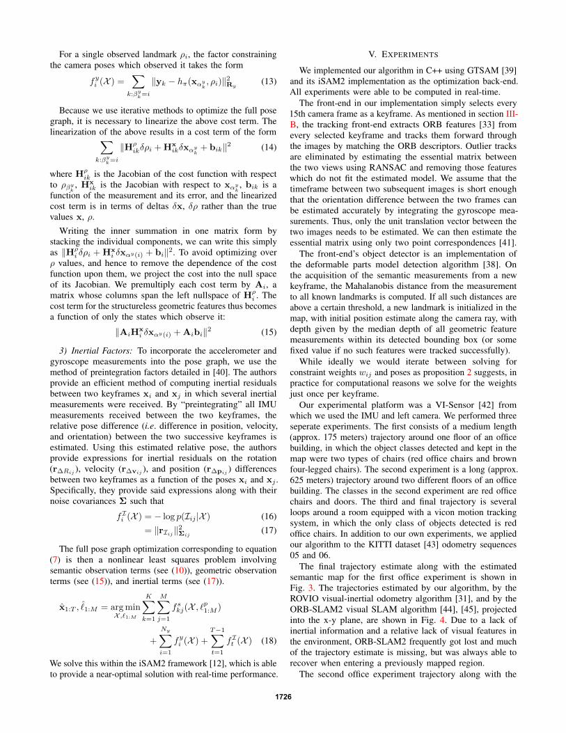
The final trajectory estimate along with the estimatedsemantic map for the first office experiment is shown inFig. 3. The trajectories estimated by our algorithm, by theROVIO visual-inertial odometry algorithm [31], and by theORB-SLAM2 visual SLAM algorithm [44], [45], projectedinto the x-y plane, are shown in Fig. 4. Due to a lack ofinertial information and a relative lack of visual features inthe environment, ORB-SLAM2 frequently got lost and muchof the trajectory estimate is missing, but was always able torecover when entering a previously mapped region.

The second office experiment trajectory along with the

1726

Fig. 3: Sensor trajectory and estimated land-marks for the first office experiment

−10 −5 0 5 10 15 20 25

0

5

10

15

20

25

x [m]

y[m

]

OursROVIOORB-SLAM2 Mono

Fig. 4: Estimated trajectories in first officeexperiment.

Fig. 5: Estimated trajectory in second officeexperiment from our algorithm (blue line)along with our estimated door landmarkpositions (blue circles), overlaid onto partialground truth map (red) along with groundtruth door locations (green squares)

estimated map is shown in Fig. 2. An example imageoverlaid with object detections from near the beginning ofthis trajectory is displayed in Fig. 1. We constructed a partialmap of the top floor in the experiment using a ground robotequipped with a lidar scanner. On this ground truth map,we manually picked out door locations. The portion of theestimated trajectory on the top floor is overlayed onto thispartial truth map (the two were manually aligned) in Fig. 5,Due to the extremely repetitive nature of the hallways inthis experiment, bag-of-words based loop closure detectionsare subject to false positives and incorrect matches. ORB-SLAM2 was unable to successfully estimate the trajectorydue to such false loop closures. A partial trajectory estimateafter an incorrect loop closure detection is shown in Fig. 6.

The vicon trajectory and the estimated map of chairs isshown in Fig. 7. We evaluated the position error with respectto the vicon’s estimate for our algorithm, ROVIO, and ORB-SLAM2 and the results are shown in Fig. 8. Note that thespikes in the estimate errors are due to momentary occlusionfrom the vicon cameras.

We also evaluated our algorithm on the KITTI outdoordataset, using odometry sequences 05 and 06. The semanticobjects detected and used in our algorithm were cars. Ratherthan use inertial odometry in this experiment, we used theVISO2 [46] visual odometry algorithm as the initial guessX (0) for a new keyframe state. Similarly, we replaced thepreintegrated inertial relative pose (cf. Sec. IV-B.3) with therelative pose obtained from VISO in the odometry factors.The absolute position errors over time for KITTI sequence 05with respect to ground truth for our algorithm, VISO2, andORB-SLAM2 with monocular and stereo cameras are shownin Fig. 9. The same for sequence 06 are shown in Fig. 10.Finally, the mean translational and rotational errors over allpossible subpaths of length (100, 200, ..., 800) meters areshown in Fig. 11.

VI. CONCLUSION

The experiments demonstrated that in complex and clut-tered real-world datasets our method can be used to recon-struct the full 6-D pose history of the sensor and the positionsand classes of the objects contained in the environment.The advantage of our work is that by having semanticfeatures directly into the optimization, we include a relativelysparse and easily distinguishable set of features that allows

for improved localization performance and loop closure,while only slightly impacting the computational cost ofthe algorithm. Furthermore, semantic information about theenvironment is valuable in and of itself in aiding autonomousoperation of robots within a human-centric environment.

In future work, we plan to expand our algorithm to estimatethe full pose of the semantic objects (i.e., orientation inaddition to position). We also plan to fully exploit our EMdecomposition by reconsidering data associations for pastkeyframes, and to consider systems with multiple sensorsand non-stationary objects.

APPENDIX I: PROOF OF PROPOSITION 1

First, we rewrite the optimization in (4) without a logarithmand similarly expand the expectation:

X i+1,Li+1=argmaxX ,L

∑D∈D

p(D|X i,Li,Z)p(Z|X ,L,D)

The data association likelihood can then be rewrite as

p(D|X i,Li,Z) = p(Z|X i,Li,D)p(D|X i,Li)∑D p(Z|X i,Li,D)p(D|X i,Li)

(19)

=p(Z|X i,Li,D)∑D p(Z|X i,Li,D)

(20)

with the last equality due to the assumption that p(D|X ,L) isuniform. We can next decompose the measurement likelihoodp(Z|X ,L,D) =∏k p(zk|xαk

, `βk), and so

X i+1,Li+1=argmaxX ,L

∑D∈D

p(D|X i,Li,Z)p(Z|X ,L,D) (21)

=argmaxX ,L

∑D∈D

∏k

p(zk|xiαk, `iβk

)p(zk|xαk, `βk

)∑D p(Z|X i,Li,D)

The result then follows by noting that the normalizingdenominator is independent of the optimization variables andfrom the definition of the matrix permanent.

APPENDIX II: PROOF OF PROPOSITION 2

Suppose we have some initial guess given by θ(i) ={X (i), `p,(i)}. We can then compute an improved estimate ofθ = {X , `p} by maximizing the expected log likelihood:

θ(i+1) = argmaxθ

ED,`c|θ(i) [log p(D, `c,S,Y, I|θ)] (22)

1727

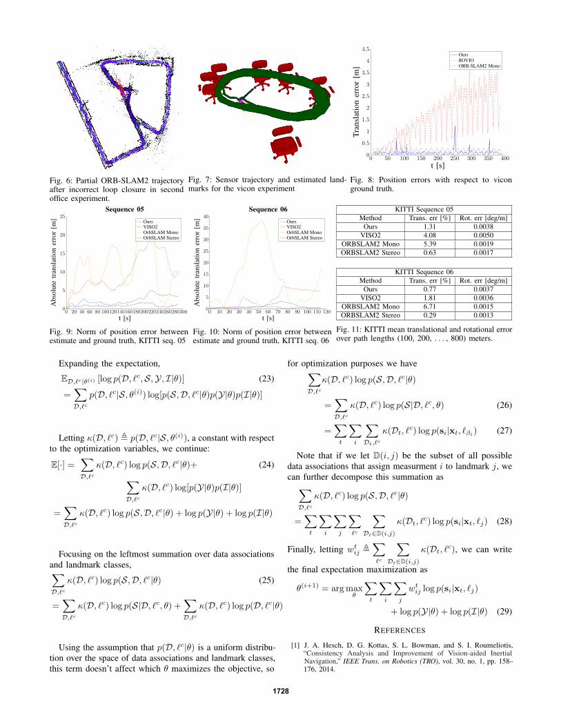
Fig. 6: Partial ORB-SLAM2 trajectoryafter incorrect loop closure in secondoffice experiment.

Fig. 7: Sensor trajectory and estimated land-marks for the vicon experiment

0 50 100 150 200 250 300 350 4000

0.5

1

1.5

2

2.5

3

3.5

4

4.5

t [s]

Tran

slat

ion

erro

r[m

]

OursROVIOORB-SLAM2 Mono

Fig. 8: Position errors with respect to viconground truth.

0 20 40 60 80 1001201401601802002202402602803000

5

10

15

20

25

t [s]

Abs

olut

etr

ansl

atio

ner

ror

[m]

Sequence 05OursVISO2OrbSLAM MonoOrbSLAM Stereo

Fig. 9: Norm of position error betweenestimate and ground truth, KITTI seq. 05

0 10 20 30 40 50 60 70 80 90 100 110 1200

5

10

15

20

25

30

35

40

t [s]

Abs

olut

etr

ansl

atio

ner

ror

[m]

Sequence 06OursVISO2OrbSLAM MonoOrbSLAM Stereo

Fig. 10: Norm of position error betweenestimate and ground truth, KITTI seq. 06

KITTI Sequence 05Method Trans. err [%] Rot. err [deg/m]

Ours 1.31 0.0038VISO2 4.08 0.0050

ORBSLAM2 Mono 5.39 0.0019ORBSLAM2 Stereo 0.63 0.0017

KITTI Sequence 06Method Trans. err [%] Rot. err [deg/m]

Ours 0.77 0.0037VISO2 1.81 0.0036

ORBSLAM2 Mono 6.71 0.0015ORBSLAM2 Stereo 0.29 0.0013

Fig. 11: KITTI mean translational and rotational errorover path lengths (100, 200, . . . , 800) meters.

Expanding the expectation,

ED,`c|θ(i) [log p(D, `c,S,Y, I|θ)] (23)

=∑D,`c

p(D, `c|S, θ(i)) log[p(S,D, `c|θ)p(Y|θ)p(I|θ)]

Letting κ(D, `c) , p(D, `c|S, θ(i)), a constant with respectto the optimization variables, we continue:

E[·] =∑D,`c

κ(D, `c) log p(S,D, `c|θ)+∑D,`c

κ(D, `c) log[p(Y|θ)p(I|θ)]

(24)

=∑D,`c

κ(D, `c) log p(S,D, `c|θ) + log p(Y|θ) + log p(I|θ)

Focusing on the leftmost summation over data associationsand landmark classes,∑D,`c

κ(D, `c) log p(S,D, `c|θ) (25)

=∑D,`c

κ(D, `c) log p(S|D, `c, θ) +∑D,`c

κ(D, `c) log p(D, `c|θ)

Using the assumption that p(D, `c|θ) is a uniform distribu-tion over the space of data associations and landmark classes,this term doesn’t affect which θ maximizes the objective, so

for optimization purposes we have∑D,`c

κ(D, `c) log p(S,D, `c|θ)

=∑D,`c

κ(D, `c) log p(S|D, `c, θ) (26)

=∑t

∑i

∑Dt,`c

κ(Dt, `c) log p(si|xt, `βi) (27)

Note that if we let D(i, j) be the subset of all possibledata associations that assign measurment i to landmark j, wecan further decompose this summation as∑D,`c

κ(D, `c) log p(S,D, `c|θ)

=∑t

∑i

∑j

∑`c

∑Dt∈D(i,j)

κ(Dt, `c) log p(si|xt, `j) (28)

Finally, letting wtij ,∑`c

∑Dt∈D(i,j)

κ(Dt, `c), we can write

the final expectation maximization as

θ(i+1) = argmaxθ

∑t

∑i

∑j

wtij log p(si|xt, `j)

+ log p(Y|θ) + log p(I|θ) (29)

REFERENCES

[1] J. A. Hesch, D. G. Kottas, S. L. Bowman, and S. I. Roumeliotis,“Consistency Analysis and Improvement of Vision-aided InertialNavigation,” IEEE Trans. on Robotics (TRO), vol. 30, no. 1, pp. 158–176, 2014.

1728

[2] D. G. Kottas and S. I. Roumeliotis, “Efficient and Consistent Vision-aided Inertial Navigation using Line Observations,” in IEEE Int. Conf.on Robotics and Automation (ICRA), 2013, pp. 1540–1547.

[3] P. Henry, M. Krainin, E. Herbst, X. Ren, and D. Fox, “RGB-D mapping:Using Kinect-style depth cameras for dense 3D modeling of indoorenvironments,” The International Journal of Robotics Research (IJRR),vol. 31, no. 5, pp. 647–663, 2012.

[4] P. Felzenszwalb, R. Girshick, D. McAllester, and D. Ramanan, “ObjectDetection with Discriminatively Trained Part-Based Models,” IEEETrans. on Pattern Analysis and Machine Intelligence (PAMI), vol. 32,no. 9, pp. 1627–1645, 2010.

[5] S. Ren, K. He, R. Girshick, and J. Sun, “Faster R-CNN: Towardsreal-time object detection with region proposal networks,” in Advancesin Neural Information Processing Systems (NIPS), 2015.

[6] P. Agrawal, R. Girshick, and J. Malik, “Analyzing the performanceof multilayer neural networks for object recognition,” in ComputerVision–ECCV 2014. Springer, 2014, pp. 329–344.

[7] X. Liu, Y. Zhao, and S.-C. Zhu, “Single-view 3d scene parsing byattributed grammar,” in Computer Vision and Pattern Recognition(CVPR), 2014 IEEE Conference on. IEEE, 2014, pp. 684–691.

[8] X. Chen, K. Kundu, Y. Zhu, A. Berneshawi, H. Ma, S. Fidler, andR. Urtasun, “3d object proposals for accurate object class detection,”in NIPS, 2015.

[9] H. Durrant-Whyte and T. Bailey, “Simultaneous localization andmapping: part i,” Robotics Automation Magazine, IEEE, vol. 13, no. 2,pp. 99–110, June 2006.

[10] F. Lu and E. Milios, “Globally Consistent Range Scan Alignment forEnvironment Mapping,” Auton. Robots, vol. 4, no. 4, pp. 333–349,1997.

[11] R. Kummerle, G. Grisetti, H. Strasdat, K. Konolige, and W. Burgard,“g2o: A General Framework for Graph Optimization,” in IEEE Int.Conf. on Robotics and Automation (ICRA), 2011, pp. 3607–3613.

[12] M. Kaess, H. Johannsson, R. Roberts, V. Ila, J. Leonard, and F. Dellaert,“iSAM2: Incremental Smoothing and Mapping Using the Bayes Tree,”The International Journal of Robotics Research (IJRR), vol. 31, no. 2,pp. 216–235, 2012.

[13] C. Galindo, A. Saffiotti, S. Coradeschi, P. Buschka, J. Fernandez-Madrigal, and J. Gonzalez, “Multi-hierarchical Semantic Maps forMobile Robotics,” in IEEE/RSJ Int. Conf. on Intelligent Robots andSystems (IROS), 2005, pp. 2278–2283.

[14] J. Civera, D. Galvez-Lopez, L. Riazuelo, J. Tardos, and J. Montiel,“Towards Semantic SLAM Using a Monocular Camera,” in IEEE/RSJInt. Conf. on Intelligent Robots and Systems, 2011, pp. 1277–1284.

[15] A. Pronobis, “Semantic Mapping with Mobile Robots,” dissertation,KTH Royal Institute of Technology, 2011.

[16] J. Stuckler, B. Waldvogel, H. Schulz, and S. Behnke, “Dense real-timemapping of object-class semantics from RGB-D video,” Journal ofReal-Time Image Processing, pp. 1–11, 2013.

[17] V. Vineet, O. Miksik, M. Lidegaard, M. Nießner, S. Golodetz, V. A.Prisacariu, O. Kahler, D. W. Murray, S. Izadi, P. Perez, and P. H. S.Torr, “Incremental dense semantic stereo fusion for large-scale semanticscene reconstruction,” in IEEE International Conference on Roboticsand Automation (ICRA), 2015.

[18] B. Leibe, N. Cornelis, K. Cornelis, and L. Van Gool, “Dynamic 3dscene analysis from a moving vehicle,” in IEEE Conf. on ComputerVision and Pattern Recognition (CVPR), June 2007, pp. 1–8.

[19] S. Pillai and J. Leonard, “Monocular slam supported object recognition,”in Proceedings of Robotics: Science and Systems (RSS), Rome, Italy,July 2015.

[20] N. Atanasov, M. Zhu, K. Daniilidis, and G. Pappas, “SemanticLocalization Via the Matrix Permanent,” in Robotics: Science andSystems (RSS), 2014.

[21] S. Bao and S. Savarese, “Semantic Structure from Motion,” in IEEEConf. on Computer Vision and Pattern Recognition (CVPR), 2011, pp.2025–2032.

[22] R. Salas-Moreno, R. Newcombe, H. Strasdat, P. Kelly, and A. Davison,“SLAM++: Simultaneous Localisation and Mapping at the Level ofObjects,” in IEEE Conf. on Computer Vision and Pattern Recognition(CVPR), 2013, pp. 1352–1359.

[23] D. Galvez-Lopez, M. Salas, J. Tardos, and J. Montiel, “Real-timeMonocular Object SLAM,” arXiv:1504.02398, 2015.

[24] I. Reid, “Towards Semantic Visual SLAM,” in Int. Conf. on ControlAutomation Robotics Vision (ICARCV), 2014.

[25] A. Kundu, Y. Li, F. Dellaert, F. Li, and J. Rehg, “Joint semanticsegmentation and 3d reconstruction from monocular video,” inComputer Vision ECCV 2014, ser. Lecture Notes in ComputerScience, D. Fleet, T. Pajdla, B. Schiele, and T. Tuytelaars, Eds.

Springer International Publishing, 2014, vol. 8694, pp. 703–718.[Online]. Available: http://dx.doi.org/10.1007/978-3-319-10599-4 45

[26] I. Kostavelis and A. Gasteratos, “Semantic mapping for mobile roboticstasks: A survey,” Robotics and Autonomous Systems, vol. 66, pp. 86–103, 2015.

[27] J. Neira and J. Tardos, “Data Association in Stochastic Mapping Usingthe Joint Compatibility Test,” IEEE Trans. on Robotics and Automation(TRO), vol. 17, no. 6, pp. 890–897, 2001.

[28] J. Munkres, “Algorithms for the Assignment and TransportationProblems,” Journal of the Society for Industrial & Applied Mathematics(SIAM), vol. 5, no. 1, pp. 32–38, 1957.

[29] N. Atanasov, M. Zhu, K. Daniilidis, and G. Pappas, “Localization fromsemantic observations via the matrix permanent,” The InternationalJournal of Robotics Research, vol. 35, no. 1-3, pp. 73–99, 2016.

[30] A. Mourikis and S. I. Roumeliotis, “A multi-state constraint kalmanfilter for vision-aided inertial navigation,” in Robotics and Automation,2007 IEEE International Conference on. IEEE, 2007, pp. 3565–3572.

[31] M. Bloesch, S. Omari, M. Hutter, and R. Siegwart, “Robust visualinertial odometry using a direct ekf-based approach,” in IEEE/RSJ Int.Conf. on Intelligent Robots and Systems (IROS), 2015, pp. 298–304.

[32] C. Forster, M. Pizzoli, and D. Scaramuzza, “Svo: Fast semi-directmonocular visual odometry,” in IEEE Int. Conf. on Robotics andAutomation (ICRA), 2014, pp. 15–22.

[33] E. Rublee, V. Rabaud, K. Konolige, and G. Bradski, “Orb: An efficientalternative to sift or surf,” in Int. Conf. on Computer Vision, 2011, pp.2564–2571.

[34] S. Gidaris and N. Komodakis, “Object detection via a multi-regionand semantic segmentation-aware cnn model,” in IEEE Int. Conf. onComputer Vision, 2015, pp. 1134–1142.

[35] K. He, X. Zhang, S. Ren, and J. Sun, “Deep residual learning forimage recognition,” arXiv preprint arXiv:1512.03385, 2015.

[36] Z. Cai, Q. Fan, R. Feris, and N. Vasconcelos, “A unified multi-scale deepconvolutional neural network for fast object detection,” in EuropeanConference on Computer Vision (ECCV), 2016.

[37] M. Zhu, N. Atanasov, G. Pappas, and K. Daniilidis, “Active DeformablePart Models Inference,” in European Conference on Computer Vision(ECCV), ser. Lecture Notes in Computer Science. Springer, 2014, vol.8695, pp. 281–296.

[38] C. Dubout and F. Fleuret, “Deformable part models with individualpart scaling,” in British Machine Vision Conference, no. EPFL-CONF-192393, 2013.

[39] F. Dellaert, “Factor graphs and gtsam: A hands-on introduction,”GT RIM, Tech. Rep. GT-RIM-CP&R-2012-002, Sept 2012.[Online]. Available: https://research.cc.gatech.edu/borg/sites/edu.borg/files/downloads/gtsam.pdf

[40] C. Forster, L. Carlone, F. Dellaert, and D. Scaramuzza, “Imu preinte-gration on manifold for efficient visual-inertial maximum-a-posterioriestimation,” in Proceedings of Robotics: Science and Systems, Rome,Italy, July 2015.

[41] D. G. Kottas, K. Wu, and S. I. Roumeliotis, “Detecting and dealingwith hovering maneuvers in vision-aided inertial navigation systems,”in 2013 IEEE/RSJ International Conference on Intelligent Robots andSystems, Nov 2013, pp. 3172–3179.

[42] J. Nikolic, J. Rehder, M. Burri, P. Gohl, S. Leutenegger, P. T. Furgale,and R. Siegwart, “A synchronized visual-inertial sensor system withfpga pre-processing for accurate real-time slam,” in Robotics andAutomation (ICRA), 2014 IEEE International Conference on. IEEE,2014, pp. 431–437.

[43] A. Geiger, P. Lenz, and R. Urtasun, “Are we ready for autonomousdriving? the kitti vision benchmark suite,” in Conference on ComputerVision and Pattern Recognition (CVPR), 2012.

[44] R. Mur-Artal, J. M. M. Montiel, and J. D. Tardos, “ORB-SLAM: aversatile and accurate monocular SLAM system,” IEEE Transactionson Robotics, vol. 31, no. 5, pp. 1147–1163, 2015.

[45] R. Mur-Artal and J. D. Tardos, “ORB-SLAM2: an open-sourceSLAM system for monocular, stereo and RGB-D cameras,”CoRR, vol. abs/1610.06475, 2016. [Online]. Available: http://arxiv.org/abs/1610.06475

[46] A. Geiger, J. Ziegler, and C. Stiller, “StereoScan: Dense 3d Recon-struction in Real-time,” in Intelligent Vehicles Symposium (IV), 2011,pp. 963–968.

1729