Principal Component Analysis - Instituto Superior de ...files.isec.pt/DOCUMENTOS/SERVICOS/BIBLIO/Documentos de acesso...11 Extensions; two-block regression and many-way tables

Tutorial n

Chemometrics and Intelligent Laboratory Systems, 2 (1987) 37-52

Elsevier Science Publishers B.V., Amsterdam - Printed in The Netherlands

Principal Component Analysis

SVANTE WOLD *

Research Group for Chemometrics, Institute of Chemistry, Umei University, S 901 87 Urned (Sweden)

KIM ESBENSEN and PAUL GELADI

Norwegian Computing Center, P.B. 335 Blindern, N 0314 Oslo 3 (Norway) and Research Group for Chemometrics, Institute of Chemistry, Umed University, S 901 87 Umeci (Sweden)

CONTENTS

Intr~uction: history of principal component analysis ...... ............... ....... Problem definition for multivariate data ................ ............... ....... A chemical example .............................. ............... ....... Geometric interpretation of principal component analysis ... ............... ....... Majestical defi~tion of principal component analysis .... ............... ....... Statistics; how to use the residuals .................... ............... ....... Plots ......................................... ............... ....... Applications of principal component analysis ............ ............... ....... 8.1 Overview (plots) of any data table ................. ............... . ..*... 8.2 Dimensionality reduction ....................... ............... . . . . . . . 8.3 Similarity models ............................. ............... . . . , . . . Data pre-treatment .............................. ............... *....s.

10 Rank, or dim~sion~ty, of a principal components model. .......................... 11 Extensions; two-block regression and many-way tables ............................. 12 Summary ............................................................. References.. ............................................................. Appendix ................................................................

1 INTRODUCTION: HISTORY OF PRINCIPAL COMPO- NENT ANALYSIS

Principal component analysis (PCA) in many ways forms the basis for multiv~ate data analysis. PCA provides an approximation of a data table, a data matrix, X, in terms of the product of two small matrices T and P’. These matrices, T and P’, capture the essential data patterns of X.

Plotting the columns of T gives a picture of the dominant “object patterns” of X and, analo-

gously, plotting the rows of P’ shows the complementary “ variable patterns”.

Consider, as an example, a data matrix containing absorbances at K = 100 frequencies measured on N = 10 mixtures of two chemical constituent. This matrix is well approximated by a (10 X 2) matrix T times a (2 x 100) matrix P’, where T describes the concentrations of the constituents and P describes their spectra.

PCA was first formulated in statistics by Pear- son [l], who formulated the analysis as finding

0169-7439/87/$03.50 0 1987 Elsevier Science Publishers B.V. 37

37 38

40

41

41

43 44

46

46

46 47

47

48

49

50

50

51

n Chemometrics and Intelligent Laboratory Systems

“lines and planes of closest fit to systems of points in space”. This geometric interpretation

will be further discussed in Section 4. PCA was briefly mentioned by Fisher and MacKenzie [2] as

more suitable than analysis of variance for the modelling of response data. Fisher and MacKen- zie also outlined the NIPALS algorithm, later

rediscovered by Wold [3]. Hotelling [4] further developed PCA to its present stage. In the 1930s the development of factor analysis (FA) was started by Thurstone and other psychologists. This needs mentioning here because FA is closely related to PCA and often the two methods are confused and the two names are incorrectly used interchangeably.

Since then, the utility of PCA has been redis-

covered in many diverse scientific fields, resulting in, amongst other things, an abundance of redun-

dant terminology. PCA now goes under many names. Apart from those already mentioned, singular value decomposition (SVD) is used in numerical analysis [5,6] and Karhunen-LoCve expansion [7,8] in electrical engineering. Eigenvector analysis and characteristic vector analysis are often used in the physical sciences. In image analysis, the term Hotelling transformation is often used for a principal component projection. Correspon- dence analysis is a special double-scaled variant of PCA that is much favoured in French-speaking countries and Canada and in some scientific fields.

Many good statistical textbooks that include this subject have been published, e.g., by Gnana- desikan [9], Mardia et al. [lo], Johnson and Wichern [ll] and Joliffe [12]. The latter is devoted solely to PCA and is strongly recommended for reading.

In chemistry, PCA was introduced by Malinowski around 1960 under the name principal factor analysis, and after 1970 a large number of chemical applications have been published (see Malinowski and Howery [13]), and Kowalski et al. [14]).

In geology, PCA has lived a more secluded life, partly overshadowed by its twin brother factor analysis (FA), which has seen ups and downs in the past 15-20 years. The one eminent textbook in this field of geological factor analysis is that by Joreskog, Klovan and Reyment [15]. Davis [16],

38

who has set the standards for statistics and data analysis in geology for more than a decade, also

included a lucid introduction to PCA.

2 PROBLEM DEFINITION FOR MULTIVARIATE DATA

The starting point in all multivariate data analysis is a data matrix (a data table) denoted by X. The N rows in the table are termed “objects”. These often correspond to chemical or geological samples. The K columns are termed “variables” and comprise the measurements made on the objects. Fig. 1 gives an overview of the different goals one can have for analysing a data matrix.

These are defined by the problem at hand and not all of them have to be considered at the same

time. Fig. 2 gives a graphical overview of the matrices

and vectors used in PCA. Many of the goals of PCA are concerned with finding relationships between objects. One may be interested, for example, in finding classes of similar objects. The class membership may be known in advance, but it may also be found by exploration of the available data. Associated with this is the detection of outliers, since outliers do not belong to known classes.

A matrix of data, measured for N

SIMPLIFICATION DATA REDUCTION

MODELING OUTLIER DETECTION

VARIABLE SELECTIOn CLASSIFICATION

PREDICTION UNMIXING

Fig. 1. Principal component analysis on a data matrix can have many goals.

Tutorial U

k K 1 t, 5

i X

N 0

E

P’, p;

[

E

X= lii+TP’+E Fig. 2. A data matrix X with its first two principal components. Index i is used for objects (rows) and index k for variables

(columns). There are N objects and K variables. The matrix E

contains the residuals, the part of the data not “explained” by the PC model.

Another goal could be data reduction. This is

useful when large amounts of data may be approximated by a moderately complex model structure.

In general, almost any data matrix can be sim- plified by PCA. A large table of numbers is one of the more difficult things for the human mind to comprehend. PCA can be used together with a well selected set of objects and variables to build a model of how a physical or chemical system be- haves, and this model can be used for prediction when new data are measured for the same system. PCA has also been used for unmixing constant sum mixtures. This branch is usually called curve

resolution [17,18]. PCA estimates the correlation structure of the

variables. The importance of a variable in a PC model is indicated by the size of its residual variance. This is often used for variable selection.

Fig. 3 gives a graphical explanation of PCA as a tool for separating an underlying systematic

Fig. 3. The data matrix X can be regarded as a combination of an underlying structure (PC model) M and noise E. The underlying structure can be known in advance or one may have

to estimate it from X.

data structure from noise. Fig. 4a and b indicate

the projection properties of PCA. With adequate interpretation, such projections reveal the domi- nating characteristics of a given multivariate data set.

Fig. 5 contains a small (3 x 4) numerical illustration that will be used as an example.

(0)

El X

lb)

clli P’ Fig. 4. (a) Projecting the matrix X into a vector I is the same as assigning a scalar to every object (row). The projection is chosen such that the values in r have desirable properties and

that the noise contributes as little as possible. (b) projecting the

matrix X into a vector p’ is the same as assigning a scalar to every variable (column). The projection is chosen such that the

values in p’ have desirable properties and that the noise contributed as little as possible.

39


4 3 4 3

5 5 6 4

scaling weights

scaled

test objects Xt

Xt -x , scaled

Fig. 5. A training data matrix used as an illustration. Two extra objects are included as a test set. The actions of mean- centring and variance-scaling are illustrated.

3 A CHEMICAL EXAMPLE

Cole and Phelps [19] presented data relating to a classical multivariate discrimination problem.

On 16 samples of fresh and stored swedes (vegeta- bles), they measured 8 chromatographic peaks. Two data classes are present: fresh swedes and swedes that have been stored for some months.

The food administration problem is clear: can we distinguish between these two categories on the basis of the chromatographic data alone?

Fig. 6 shows the PC score plot (explained later) for all 16 samples. Two strong features stand out: sample 7 is an outlier and the two classes, fresh and stored, are indeed separated from each other. Fig. 7 shows the corresponding plot calculated on the reduced data set where object 7 has been deleted. Here the separation between these two

40

0

0

w 0

Fig. 6. Plot of the first two PC score vectors (t, and 1s) of the Swede data of Cole and Phelps [19]. The data were logarithmed and centred but not scaled before the analysis. Objects l-7 and 15 are fresh samples, whereas 8-14 and 16 are stored samples.

data classes is even better. Further details of the analysis of this particular data set will be given

below.

M 0

A

Fig. 7. PC plot of the same data as in Fig. 6 but calculated after object 7 was deleted.

Tutorial n

4 GEOMETRIC INTERPRETATION OF PRINCIPAL COMPONENT ANALYSIS

A data matrix X with N objects and K variables can be represented as an ensemble of N points in a K-dimensional space. This space may be termed M-space for measurement space or multivariate space or K-space to indicate its dimensionality. An M-space is difficult to visualize when K > 3. However, mathematically, such a space is similar to a space with only two or three dimensions. Geometrical concepts such as points, lines, planes, distances and angles all have the same properties in M-space as in 3-space. As a demonstration, consider the following BASIC program, which calculates the distance between the two points Z and J in 3-space:

100 KDIM = 3

110 DIST = 0

120 FOR L = 1 TO KDIM

130 DIST = DIST + (X(1, L) - X(J, L)) * *2

140 NEXT L

150 DIST = SQR(DIST)

How can be change this program to calculate the distance between two points in a space with, say, 7 or 156 dimensions? Simply change statement 100 to KDIM = 7 or KDIM = 156.

A straight line with direction coefficients P(K) passing through a point with coordinates C(E() has the same equation in any linear space. All points (I) on the line have coordinates X( I, K) obeying the relationship (again in BASIC nota- tion)

X(1, K) = C(K) + T(1) *P(K)

Hence, one can use 2-spaces and 3-spaces as illus- trations for what happens in any space we discuss henceforth. Fig. 8 shows a 3-space with a point swarm approximated by a one-component PC model: a straight line. A two-component PC model is a plane - defined by two orthogonal lines - and an A-components PC model is an A-dimensional hyperplane. From Fig. 8 it may be realized that the fitting of a principal component line to a number of data points is a least squares process.

Lines, planes and hyperplanes can be seen as

31:

1

1

Fig. 8. A data matrix X is represented as a swarm with N Points in a K-dimensional space. This figure shows a 3-space

with a straight line fitted to the points: a one-component PC model. The PC score of an object ( ri) is its orthogonal projec-

tion on the PC line. The direction coefficients of the line from

the loading vector pk.

spaces with one, two and more dimensions. Hence,

we can see PCA also as the projection of a point swarm in M-space down on a lower-dimensional subspace with A dimensions.

Another way to think about PCA is to regard the subspaces as a windows into M-space. The data are projected on to the window, which gives a picture of their configuration in M-space.

5 MATHEMATICAL DEFINITION OF PRINCIPAL COM- PONENT ANALYSIS

The projection of X down on an A-dimensional subspace by means of the projection matrix P’ gives the object coordinates in this plane, T. The columns in T, f,, are called score vectors and the rows in P’, pi, are called loading vectors. The latter comprise the direction coefficients of the PC (hyper) plane. The vectors r, and p. are orthogonal, i.e., p,!pj = 0 and t,!tj = 0, for i f j.

The deviations between projections and the original coordinates are termed the residuals. These

41

W Chemometrics and Intelligent Laboratory Systems

are collected in the matrix E. PCA in matrix form

is the least squares model:

X=lx+TP’+E

Here the mean vector X is explicitly included in the model formulation, but this is not mandatory. The data may be projected on a hyperplane passing through the origin. Fig. 9 gives a graphical representation of this formula.

The sizes of the vectors t, and p, in a PC

dimension are undefined with respect to a multi- plicative constant, c, as tp = (tc)( p/c). Hence it is necessary to anchor the solution in some way. This is usually done by normalizing the vectors p, to length 1.0. In addition, it is useful to constrain its largest element to be positive. In this way, the ambiguity for c = - 1 is removed.

An anchoring often used in FA is to have the

length of p, be the square root of the corresponding eigenvalue I,. This makes the elements in p, correspond directly to correlation coefficients and the score vectors t, be standardized to length 1.0.

It is instructive to make a comparison with the

singular value decomposition (SVD) formulation:

X=l.f+UDV’+E

In this instance, V’ is identical with P’. U con-

tains the same column vectors as does T, but normalized to length one. D is a diagonal matrix containing the lengths of the column vectors of T. These diagonal elements of D are the square roots

of the eigenvalues of X’X. In the statistical literature, PCA has two slightly

different meanings. Traditionally, PCA has been

Fig. 9. A data matrix X can be decomposed as a sum of matrices Mi and a residual E. The M, can be seen as consist- ing of outer products of a score vector t, and a loading vector

, PI.

viewed as an expansion of X in as many components as min(N, K). This corresponds to ex-

pressing X in new orthogonal variables, i.e., a transformation to a new coordinate system. The one which is discussed here refers to PCA as the approximation of the matrix X by a model with a relatively small number of columns in T and P. The possibility of deciding on a specific cut-off of the number of components gives a flexible tool for problem-dependent data analysis: several contributions to this issue make ample use of these PCA facilities.

A basic assumption in the use of PCA is that the score and loading vectors corresponding to the largest eigenvalues contain the most useful information relating to the specific problem, and that the remaining ones mainly comprise noise. There-

fore, these vectors are usually written in order of descending eigenvalues.

Often the obtained PC model is rotated by the rotation matrix R to make the scores and loading easier to interpret. This is possible because of the

equivalence

TP’ = m-‘P’ = SQ’

The FA literature contains numerous discussions about various rotation schemes, which we refrain from adding to here because the choice of rotation is very problem specific and often problematic.

Once the PC model has been developed for a “training matrix”, new objects or variables may be fitted to the model giving scores, t, for the new objects, or loadings, p, for the new variables, respectively. In addition, the variance of the residuals, e, is obtained for each fitted item, providing a measure of similarity between the item and the “training data”. If this residual variance is larger

than that found in the training stage, it can be

concluded that the new object (or variable) does not belong to the training population. Hypothesis tests can be applied to this situation. The residuals may alternatively be interpreted as residual distances with respect to a pertinent PC model.

The formulae for a new object x are as follows: multiply by the loadings from the training stage of obtain the estimated scores t:

t=xP

42

Tutorial n

Factor Analysis Eigenvalues

ExplaIned SS

54.9 % ’ q Explained Variance 45.1 % 2

Fig. 10. Results for the PC model built from the training set in Fig. 5.

x is projected into the A-dimensional space that was developed in the training stage.

Calculated the residuals vector e:

e-x-rP’ore=x(I-PP’)

Here I is the identity matrix of size K. This

calculation of the new scores t, or loadings p, is equivalent to linear regression because of the or-

thogonality of the vectors. Figs. 10 and 11 show the results of a PCA of

the (3 X 4) matrix in Fig. 5.

Traimng

Test

Fig. 11. Scores obtained for training and test set in Fig. 5.

6 STATISTICS; HOW TO USE THE RESIDUALS

This section describes two different, but related, statistics of a data matrix and its residuals, the usual variance statistics and influence statistics

(leverage). The amount of explained variance can be ex-

pressed in different ways. In FA the data are

always scaled to unit variance and the loadings are traditionally calculated by diagonalization of the

correlation matrix X’X. To obtain a measure corresponding to the factor analytical eigenvalue, in

PCA one may calculate the fraction of the explained sum of squares (SS) multiplied by the number of variables, K. Thus, in Fig. 13 the first PC explains 83.1% of the SS. Hence the first eigenvalue is 0.831 X 4 = 3.324.

For a centred matrix (column means subtracted), the variance is the sum of squares (SS) divided by the number of degrees of freedom. Sums of squares can be calculated for the matrix X and the residuals E. The number of degrees of freedom depends on the number of PC dimensions calculated. It is (N - A - l)( K - A) for the

Ath dimension when the data have been centred (column averages subtracted), otherwise (N -

A)( K - A). It is also practical to list the residual variance and modelling power for each variable (see Fig. 10).

The modeling power is defined as explained standard deviation per variable (1 - s,Js~~)_ A variable is completely relevant when its modeling power is 1. Variables with a low modeling power, below ca. (A/K), are of little relevance. This follows from the eigenvalue larger than one rule of significance (see below).

The total sum of squares and the sums of squares over rows and columns can all be used to calculate variance statistics. These can be shown as histograms and allow one to follow the evolution of the PCA model as more dimensions are calculated. Fig. 12 gives an idea of how this would look in the case of variable statistics.

The topic of influential data has been introduced recently, mainly in multiple regression analysis [20-231. A measure of influence that can be visualized geometrically is leverage. The term leverage is based on the Archimedian idea that

43


UNEXPLAINED VARIANCE

PC 0

PC I

I PC2

IPC3

VARIABLE NURSER --)

Fig. 12. Statistics for the variables. The data are shown as

histogram bars representing the variance per variable for

mean-centred and variance-scaled data. With 0 PCs, all varia-

bles have the same variance. For PC models with increasing

dimensionality, the variance of the variables is used up. The hatched bar shows a variable that contributes little to the PC

model. A similar reasoning can be. used for object variances.

anything can be lifted out of balance if the lifter has a long enough lever.

The least squares method used for fitting principal components to object points in M-space makes leverage useful for PCA. Fig. 13 shows an

Fig. 13. Leverage. A point of high leverage (indicated by a square) can rotate the principal component axis over an angle

rb.

illustration of the effect of a high leverage point on a principal component. It can be seen that high leverage is not necessarily bad. A high leverage observation falling near a PC axis only reinforces the PC model. A high leverage observation lying far away from a PC line causes a rotation of the PC.

Leverage is calculated as follows [24,25]:

Ha = T(T’T) -IT’

The diagonal element tr,, of He is the leverage for the i th object. The hi values are between 0 and 1.

For the variables, leverage is calculated as

H, = PP’

The diagonal elements h,, of JZ, are the leverages for the variables.

The interpretation of leverage is closely related to the concepts of outliers and of construction of a set of samples, i.e., the experimental (or sampling) design.

7 PLOTS

Perhaps the most common use of PCA is in the conversion of a data matrix to a few informative plots. By plotting the columns t, in the score matrix T against each other, one obtains a picture of the objects and their configuration in M-space. The first few component plots, the i,-t, or t,-t,, etc., display the most dominant patterns in X. As was commented upon above, this tacitly assumes that the directions of maximum variance represent the directions of m~mum info~ation, This need not apply to all types of data sets, but it is a well substantiated empirical finding.

Fig. 14 shows the loading plot corresponding to fig. 6 for the swedes example. In this plot one can directly identify which variables cause No. 7 to be an outlier and which variables are responsible for the separation of the two classes, fresh and stored. The directions in Fig. 6 correspond directly to the directions in Fig. 14. The horizontal direction separates No. 7 from the others in Fig. 6. Hence, variables far from zero in the horizontal direction in Fig. 14 (Nos. 5 and 6) are those responsible for this. Analogously, the vertical direction in Fig. 6

44

Tutorial W

Loading plot (pi-p21 of log SWEDES

2

1 N 0

0

-1

Da

D2

D5

Fig. 14. Plot of the first two loading vectors (p, and p2) corresponding to Fig. 6.

N P

pf

Merged score and loading plots of log SWEOES

1.7

1.6

i.6

i.4

i.3

i.2 t i., -

I .a

-

.9 -

.6 - 014

.7 - .5

.6 011 -

.5 -

.4 - .3 -

Q&g

.2 - Qi3

.1 - 0 _ 05 oi2

05 .2 -.i

-.2 - -.I - 02

-.4 -

-.I - -.6 - .6

-.7 -

-.6 -

t1 pi

Fig. 15. Figs. 6 and 14 superimposed (origin in the same place). The loadings (triangles) are scaled up by a factor of 3.

45


separates the two classes. Hence, variables verti- cally far from zero in Fig. 7 (all except No. 2, but mainly 1, 3, 7 and 8) contribute to this separation.

One may also superimpose these two plots (Figs. 6 and 14) to obtain Fig. 15, which simultaneously displays both the objects and the variables. This type of plot is common in correspondence analysis, but can also be accomplished by ordinary

PCA. It is largely a matter of choice whether one

wishes to inspect these two complementary plots in one or two separate figures. For larger data sets it is probably best to keep the two plots separate

to improve clarity.

8 APPLICATIONS OF PRINCIPAL COMPONENT ANAL- YSIS

PCA can be applied to any data matrix (properly transformed and scaled, see Section 9). This is also recommended as an initial step of any multivariate analysis to obtain a first look at the structure of the data, to help identify outliers, delineate

classes, etc. However, when the objective is classification (pattern recognition levels 1 or 2 [26]) or relating one set of variables to another (e.g., calibration), there are extensions of PCA that are more efficient for these problems.

Here a rather partisan view of PCA is presented. It reflects the experience that well considered projections encompass a surprisingly large range of typical scientific problem formulations

[27,28].

8.1 Overview (plots) of any data table

The score plot of the first two or three score vectors, 1,) shows groupings, outliers and other

strong patterns in the data. This can be seen in the score plot of the swedes data. Many other applications can be found in this issue.

8.2 Dimensionality reduction

As pointed out by Frank and Kowalski [29], two main groups of FA and PCA applications can be seen in analytical chemistry, namely the extraction of the underlying factors - the latent variables - and the resolution of spectra of multi-

46

component mixtures. In two-dimensional high-

performance liquid chromatographic analysis, for instance, this is a way to find the smallest number of species in a sample. Reviews of the numerous applications of these types can be found in

Kowalski et al. [14] and Malinowski and Howery

1131. The first few score vectors, t,, may be seen as

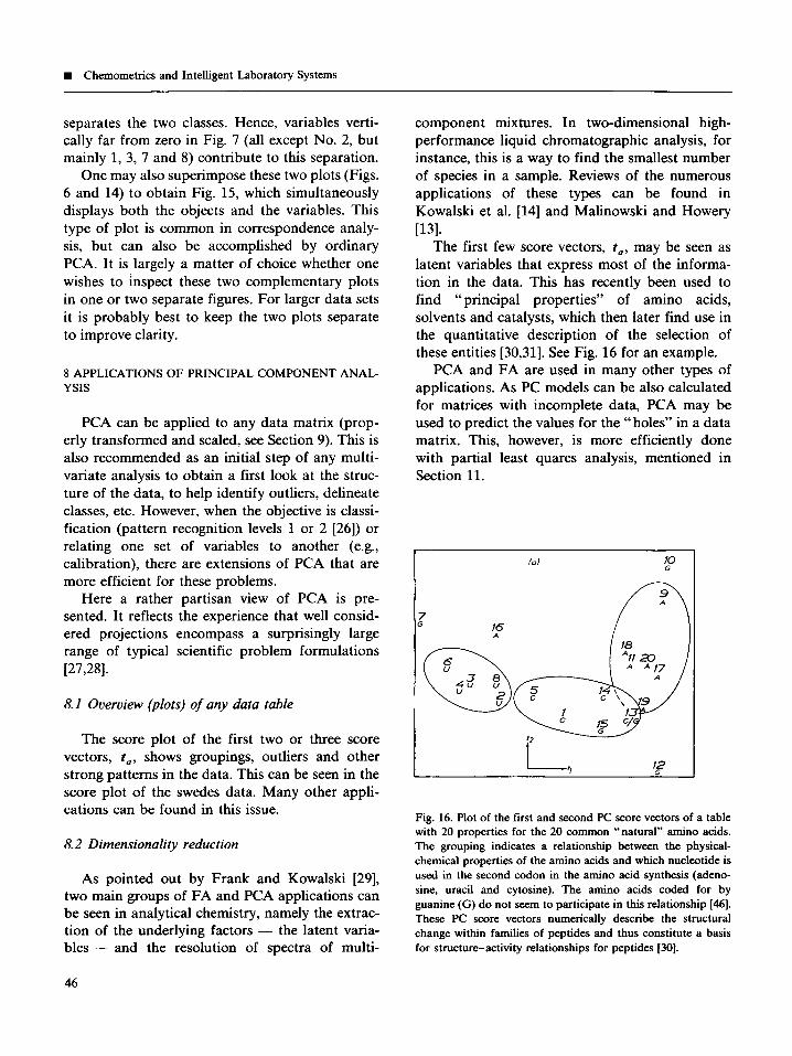
latent variables that express most of the information in the data. This has recently been used to find “principal properties” of amino acids, solvents and catalysts, which then later find use in the quantitative description of the selection of these entities [30,31]. See Fig. 16 for an example.

PCA and FA are used in many other types of applications. As PC models can be also calculated

for matrices with incomplete data, PCA may be used to predict the values for the “holes” in a data matrix. This, however, is more efficiently done with partial least quares analysis, mentioned in

Section 11.

7 t 16

*

Fig. 16. Plot of the first and second PC score vectors of a table with 20 properties for the 20 common “natural” amino acids. The grouping indicates a relationship between the physical- chemical properties of the amino acids and which nucleotide is used in the second codon in the amino acid synthesis (adeno-

sine, uracil and cytosine). The amino acids coded for by guanine (G) do not seem to participate in this relationship [46]. These PC score vectors numerically describe the structural change within families of peptides and thus constitute a basis

for structure-activity relationships for peptides 1301.

Tutorial n

8.3 Similarity models

Wold [32] showed that a PC model has the same approximation property for a data table of similar objects as does a polynomial for bivariate data in a limited interval; the PC model can be seen as a Taylor expansion of a data table. The closer the similarity between the objects, the fewer terms are needed in the expansion to achieve a certain approximation goodness. The prerequisites for this interpretation of PCA are a few assump-

tions about differentiability and continuity of the data generating process, which have been found to hold in many instances. This explains, at least partly, the practical utility of PCA.

Hence, a pattern recognition method may be based on separate PC models, one for each class

of objects. New objects are classified according to their fit or lack of fit to the class models, which gives a probabilistic classification. This is the basis for the SIMCA method (Soft Independent Model- ing of Class Analogies) [33]. If one wishes to distinguish optimally between the two classes of swedes, a PC model can be fitted to each of the classes. The results show that indeed there is similarity within the classes (two- or three-component models adequately describe the data) and that the classes are well separated (fresh samples fit the “stored class” badly and vice versa); see Wold et al. [34].

9 DATA PRE-TREATMENT

The principal components model parameters depend on the data matrix, its transformation and its scaling. Hence, these must be explicitly defined.

First, the data matrix: In statistics it is usually customary to put all available data into the matrix and analyse the lot. This conforms with the convention that all data reflect legitimate phe- nomena that have been sampled. When one has full control over the sampling, or over the experimental design, this approach may be correct.

Practical experience from many sciences often outlines a less ideal reality, however. One is fre- quently faced with outlying data in real data sets.

One also often knows certain pertinent external

facts (such that cannot be coded into the data matrix itself) relating to the problem formulation.

In chemistry, for example, one often has one set of objects (e.g., analytical samples) about which certain essential properties are known. In the swedes example, for instance, there were 16 samples that were known or assumed to be either fresh or stored. The analysis confirmed this, but the PCA recognized that one sample did not comply. This type of external information can be used to com- pute a polished PC model. On may subsequently investigate new objects and project them on to the same scores plot without letting the new samples influence the PC model as such.

Hence, it is practical to distinguish between a training set that is used for calculating problem-

dependent PC models and a test set of objects that are later subjected to the same projection as that

developed in the training phase. From the least squares formulation of the PC

models above it is seen that the scores, t, can be viewed as linear combinations of the data with the

coefficients p’. Conversely, the loadings, p’, can also to be understood as linear combinations of the data with the coefficients t. This duality has resulted in the coining of the term bilinear modeling (BLM) [35]. From this follows that if one wishes to have precise r-values, i.e., precise information about the objects, one should have many variables per object and vice versa. The rule for multiple regression that the number of variables must be much smaller that the number of objects does not apply to PCA.

As PCA is a least squares method, outlier severely influence the model. Hence it is essential to find and correct or eliminate outliers before the final PC model is developed. This is easily done by means of a few initial PC plots; outliers that have a critical influence on the model will reveal themselves clearly. Irrelevant variables can also be identified by an initial PC analysis (after taking care of outliers). Variables with little explained

variance may be removed without changing the PC model. However, usually it does not matter if they are left in. The reduction of the data set should be made only if there is a cost (computa- tional or experimental) connected with keeping the variables in the model.

41


Second, the data matrix can be subjected to transformations that make the data more symmet- rically distributed, such as a logarithmic transformation, which was used in the swedes example above. Taking the logarithm of positively skewed

data makes the tail of the data distribution shrink, often making the data more centrally distributed.

This is commonly done with chromatographic data and trace element concentration data. Autocorre- lation or Fourier transforms are recommended if

mass spectrometric data are used for classification purposes [36]. There exist a great many potential transformations that may be useful in specialized contexts. Generally, one should exercise some dis- cipline in applying univariate transformations with different parameters for different variables, lest a “shear” be introduced in the transformed covari- ante (correlation) matrix relative to that pertain-

ing to the original data. Centring the data by subtracting the column

averages corresponds to moving the coordinate system to the centre of the data.

Third, the scaling of the data matrix must be specified. Geometrically, this corresponds to

changing the length of the coordinate axes. The scaling is essential because PCA is a least squares method, which makes variables with large variance have large loadings. To avoid this bias, it is customary to standardize the data matrix so that each column has a variance 1.0. This variance scaling makes all coordinate axes have the same length, giving each variable the same influence on the PC model. This is reasonable in the first stages of a multivariate data analysis. This scaling makes the PC loadings be eigenvectors of the correlation matrix.

Variance scaling can be recommended in most instances, but some care must be taken if variables

that are almost constant have been included in the data set. The scaling will then scale up these variables substantially. If the variation of these variables is merely noise, this noise will be scaled up to be more influential in the analysis. Rule: If the standard deviation of a variable over the data set is smaller than about four times its error of measurement, leave that variable unscaled. The other variables may still be variance scaled if so desired.

When different types of variables are present,

48

say 6 infrared absorbances and 55 gas chromatographic peak sizes, a blockwise scaling may be performed so that the total variance is the same for each type of variables with autoscaling within

each block. This is accomplished by dividing each variable by is standard deviation times the square root of the number of variables of that type in the

block.

When both objects and variables are centred and normalized to unit variance, the PCA of this

derived matrix is called correspondence analysis. In correspondence analysis the “sizes” of the objects are removed from the model. This may be desirable in some applications, e.g., contingency tables and the like, but certainly not in general. This double-scaling/ centring in effect brings about a complete equivalence between variables and objects, which can confuse the interpretation of the results of the data analysis. The loading and score plots can now be superimposed. However, with proper scaling this can also be done with ordinary PCA, as shown in Fig. 15.

The treatment of missing data forms a special topic here. There may often be “holes” in the data matrix. The treatment of these can proceed mainly

in two ways. One is to “guess” a value from knowledge of the population of objects or of the properties of the measuring instrument. A simple

guess that does not affect the PCA result too much is to replace the missing value with the average for the rest of the column. Secondly, the PC algorithm may be able to cope with missing values (see Appendix). This allows the calculation of a model without having to fill in the missing value.

No matter how missing values are dealt with, an evaluation of the residuals can give extra hints.

Objects (or variables) with missing values that show up as outliers are to be treated with suspi- cion. As a rule of thumb, one can state that each object and variable should have more than five defined values per PC dimension.

10 RANK, OR DIMENSIONALITY, OF A PRINCIPAL

COMPONENTS MODEL

When PCA is used as an exploratory took, the first two or three components are always ex-

Tutorial n

tracted. These are used for studying the data structure in terms of plots. In many instances this serves well to clean the data of typing errors, sampling errors, etc. This process sometimes must be carried out iteratively in several rounds in order to pick out successively less outlying data.

When the purpose is to have a model of X, however, the correct number of components, A, is essential. Several criteria may be used to de- termine A.

It should be pointed out here that rank and dimensionality are not used in the strict mathematical sense. The ideal case is to have a number A of eigenvalues different from zero [A smaller or equal to min( K, N)] and all the others being zero. Measurement noise, sampling noise or other irreg- ularities cause almost all data matrices to be of full rank [A = min( K, N)]. This is the most difficult aspect of using PC models on “noisy” data sets.

Often, as many components are extracted as are needed to make the variance of the residual of the same size as the error of measurement of the data in X. However, this is based on the assumption that all systematic chemical and physical vari- ations in X can be explained by a PC model, an assumption that is often dubious. Variables can be very precise and still contain very little chemical information. Therefore, some statistical criterion is needed to estimate A.

A criterion that is popular, especially in FA, is to use factors with eigenvalues larger than one. This corresponds to using PCs explaining at least one K th of the total sum of squares, where K is the number of variables. This, in turn, ensures that the PCs used in the model have contributions from at least two variables. Joreskog et al. [15] discussed aspects in more detail.

Malinowski and Howery [13] and others have proposed several criteria based on the rate of decrease of the remaining residual sum of squares, but these criteria are not well understood theoreti- cally and should be used with caution [10,15].

Criteria based on bootstrapping and cross- validation (CV) have been developed for statistical model testing 1371. Bootstrapping uses the residuals to simulate a large number of data sets similar to the original and thereafter to study the distribu-

tion of the model parameters over these data. With CV the idea is to keep parts of the data

out of the model development, then predict the kept out data by the model, and finally compare the predicted values with the actual values. The squared differences between predicted and ob- served values are summed to form the prediction sum of squares (PRESS).

This procedure is repeated several times, keeping out different parts of the data until each data element has been kept out once and only once and thus PRESS has one contribution from each data element. PRESS then is a measure of the predic- tive power of the tested model.

In PCA, CV is made for consecutive model dimensions starting with A = 0. For each ad- ditional dimension, CV gives a PRESS, which is compared with the error one would obtain by just guessing the values of the data elements, namely the residual sum of squares (RSS) of the previous dimension. When PRESS is not significantly smaller than RSS, the tested dimension is considered insi~ficant and the model building is stopped.

CV for PCA was first developed by Wold [38], using the NIPALS algorithm (see Appendix) and later by Eastment and Krzanowski [39], using SVD for the computations. Experience shows that this method works well and that with the proper algorit~s it is not too computation~ly demand- ing. CV is slightly conservative, i.e., leads to too few components rather than too many. In practical work, this is an advantage in that the data are not ove~nte~reted and false leads are not created.

11 EXTENSIONS; TWO-BLOCK REGRESSION AND MANY-WAY TABLES

PCA can be extended to data matrices divided into two or more blocks of variables and is then called partial least squares (PLS) analysis (partial least squares projection to latent structures). The two-block PLS regression is related to multiple linear regression, but PLS applies also to the case with several Y-variables. See, e.g., Geladi and Kowalski [40], for a tutorial on PLS. Wold et al. [41] detailed the theoretical background for PLS

49

n Chcmometrics and Intelligent Laboratory Systems

regression. Several contributions to the present issue illustrate the diverse application potential for PLS modeling and prediction.

Multivariate image analysis can use PCA be- neficially, as explained by Esbensen et al. [42]. Multivariate image analysis is important in the chemical laboratory [43] and Geographical Infor- mation Systems (GIS).

PCA and PLS have been extended to three-way and higher order matrices by Lohmiiller and Wold 1441, and others. See the expository article by Wold et al. [45] for the theoretical background and application possibilities for these new bilinear concepts.

12 SUMMARY

Principal component analysis of a data matrix extracts the dominant patterns in the matrix in terms of a complementary set of score and loading plots. It is the r~ponsibility of the data analyst to formulate the scientific issue at hand in terms of PC projections, PLS regressions, etc. Ask yourself, or the investigator, why the data matrix was collected, and for what purpose the experiments and measurements were made. Specify before the analysis what kinds of patterns you would expect and what you would find exciting.

The results of the analysis depend on the scaling of the matrix, which therefore must be specified. Variance scaling, where each variable is scaled to unit variance, can be recommended for general use, provided that almost constant variables are left unscaled. Combining different types of variables warrants blockscaling.

In the initial analysis, look for outliers and strong groupings in the plots, indicating that the data matrix perhaps should be “polished” or whether disjoint modeling is the proper course.

For plotting purposes, two or three principal components are usually sufficient, but for modeling purposes the number of significant components should be properly determined, e.g. by cross-validation.

Use the resulting principal components to guide your continued investigation or chemical experi- mentation, not as an end in itself.

50

APPENDIX

Denoting the centred and scaled data matrix by U, the loading vectors p, are eigenvectors to the covariance matrix U'U and the score vectors t, are eigenvectors to the association matrix UU’. Therefore, principal components have earlier been computed by diagonalizing U’U or UU’. How- ever, singular value decomposition [5] is more efficient when all PCs are desired, while the NIPALS method ]3] is faster if just the first few PCs are to be computed. The NIPALS algorithm is so simple that it can be formulated in a few lines of programming and also gives an interesting interpretation of vector-matrix multiplication as the partial least squares estimation of a slope. The NIPALS algorithm also has the advantage of working for matrices with moderate amounts of randomly distributed missing observations.

The algorithm is as follows. First, scale the data matrix X and subtract the column averages if desired. Then, for each dimension, u:

(i) From a start for the score vector t, e.g., the column in X with the largest variance.

(ii) Calculate a loading vector as p’ = t’X/t’t. The elements in p can be interpreted as the slopes in the linear regressions (without intercept) of t on the corresponding column in X.

(iii) Normalize p to length one by multiplying by c = l/e (or anchor it otherwise).

(iv) Calculate a new score vector 2 = Xp/p’p. The ith element in t can be interpreted as the slope in the linear regression of p’ on the ith row in X.

(v) Check the convergence, for instance using the sum of squared differences between all elements in two consecutive score vectors. If convergence, continue with step vi, otherwise return to step ii. If convergence has not been reached in, say, 25 iterations, break anyway. The data are then almost (h~er)spheri~, with no strongly preferred direction of maximum variance.

(vi) Form the residual E = X - tp’. Use E as X in the next dimension.

Inserting the expression for t in step iv into step ii gives p = X’Xp * c/t’t (c is the normaliza- tion constant in step iii). Hence p is an eigenvector to X’X with the eigenvalue t’t/c and we see

Tutorial n

that the NIPALS algorithm is a variant of the power method used for matrix diagonalization (see, e.g., Golub and VanLoan [5]). As indicated previously, the eigenvalue is the amount of variance explained by the corresponding component multiplied by the number of variables, K.

REFERENCES

1

2

3

4

8

9

10

11

12

13

14

15

16

17

18

19

K. Pearson, On lines and planes of closest fit to systems of points in space, Philosophical Magazine, (6) 2 (1901)

559-572. R. Fisher and W. MacKenzie, Studies in crop variation. II. The manurial response of different potato varieties, Journal of Agricultural Science, 13 (1923) 311-320 H. Wold, Nonlinear estimation by iterative least squares procedures, in F. David (Editor), Research Papers in Statis-

tics, Wiley, New York, 1966, pp. 411-444.

H. Hotelling, Analysis of a compfex of statistical variables into principal #m~nents, Journal of E~catjonaf Psy-

chology, 24 (1933) 417-441 and 498520. G. Gdub and C. VanLoan, Matrix Computations, The Johns Hopkins University Press, Oxford, 1983. J. Mandel, Use of the singular value decomposition in regression analysis, American Statistician, 36 (1982) 15-24. K. Karhunen, Uber lineare Methoden in der Wahrschein- lichkeitsrechnung, Annales Acudemiae Scientiarum Fenni-

cae, Series A, 137 (1947). M. Lobe, Fonctions aleatoires de seconde ordre, in P. Levy (Editor), Processes Stochastiques et Mouvement Brownien,

Hermann, Paris, 1948. R. Gnanadesikan, Methods for Statistical Data Analysis of Multivariate Observations, Wiley, New York, 1977. K. Mardia, J. Kent and J. Bibby, ~ultiva~ute AnuZysis,

Academic Press, London, 1979. R. Johnson and D. Wichem, Applied Multivariate Statisti-

cal Analysis, Prentice-Hall, Englewood Cliffs, NJ, 1982. J. Johffe, Principal Component Analysis, Springer, Berlin, 1986. F. Malinowski and D. Howery, Factor Analysis in Chem-

istry, Wiley, New York, 1980. L.S. Ramos, K.R. Beebe, W.P. Carey, E. Sanchez, B.C. Erickson, B.E. Wilson, L.E. Wangen and B.R. Kowalski, Chemometrics, Analytical Chemistry, 58 (1986) 294R-315R. K. Jareskog, J. Klovan and R. Reyment, Geological Factor Analysis, Elsevier, Amsterdam, 1976. J. Davis, Statistics and Data Analysis in Geology, Wiley, New York, 1973 and 1986. W. Lawton and E. Sylvestre, Self modeling curve resolution, Technometrics, 13 (1971) 617-633. W. Full, R. Ehrlich and J. Klovan, Extended Q model - Objective definition of external end members in the analysis of mixtures, Mathe~t~caI Geology, 13 (1981) 331-334. R. Cole and K. Phelps, Use of canonical variate analysis in the differentiation of Swede cultivars by gas-liquid chro-

20

21

22

23

24

25

26

27

28

29

30

31

32

33

34

35

36

matography of volatile hydrolysis products, Journal of the Science of Food and Agriculture, 30 (1979) 669-676.

R. Hocking, Developments in linear regression methodol- ogy: 1959-1982, Technometrics, 25 (1983) 219-230.

R. Beckman and R. Cook, Outlier...~, Technometrics, 25

(1983) 119-149.

D. Belsley, E. Kuh and R. Welsch, Zdenti~ing Zn~uentiu~

Data and Sources of Collinearity, Wiley, new York, 1980. D. Cook and S. Weisber, Residuals and Znfluence in Regres- sion, Chapman and Hall, New York, 1982. P. Velleman and R. Welsch, Efficient computing a regression diagnostics, American Statistician, 35 (1981) 234-242. H. Martens, Mu~tivuriate Calibration, Thesis, University of Trondheim, 1985. C. Albano, W. Dunn, U. Edlund, E. Johansson, B. Horden, M. SjBstrSm and S. Weld, Four levels of pattern recognition, Analytica Chimica Acta, 103 (1978) 429-443. S. Weld, C. Albano, W. Dunn, U. Edlund, K. Esbensen, P. Geladi, S. Hellberg, E. Johansson, W. Lindberg and M. Sjiistrom, Multivariate data analysis in chemistry, in B.R. Kowalski (Editor), Chemometrics: Mathematics and Statis-

tics in Chemistry, Reidel, Dordrecht, 1984, pp. 17-95. S. Weld, C. Albano, W.J. Dunn III, K. Esbensen, P. Geladi, S. Hellberg, E. Johansson, W. Lindberg, M. Sj&triim, B. Skagerberg, C. Wikstrijm and J. Ghman, Mul- tivatiate data anatysis: Converting chemical data tables to plots, in I. Ugi and J. Brandt (Editors), Proceeding of the 7th International Conference on Computers in Chemical Re-

search and Education (ZCCCREJ, held in Garmisch-Parten-

kirchen, BDR, June 10-14, 1985, in press. I. Frank and B.R. Kowalski, Chemometrics, Analytical

Chemistry, 54 (1982) 232R-243R. S. Hellberg, M. SjijstrCm and S. Wold, The prediction of bradykinin potentiating potency of pentapeptides. An example of a peptide quantitative structure-activity relationship, Acta Chemica Scandinavica, Series B, 40 (1986) 135-140. R. Carbon, T. Lundstedt and C. Albano, Screening of suitable solvents in organic synthesis. Strategies for solvent selection, Acta Chemica Scandinaviea, Series B, 39 (1985) 79-84.

S. Weld. A theoretical foundation of extrathe~~yn~c relationships (linear free energy relationships), Chemica

Scripta, 5 (1974) 97-106. S. Wold, Pattern recognition by means of disjoint principal components models, Pattern Recognition, 8 (1976) 127-139. S. Wold, C. Albano, W. Dunn, K. Esbensen, S. Hellberg, E. Johansson and M. Sjostrom, Pattern recognition; finding and using regularities in multivariate data, in H. Martens and H. Russwurm (Editors), Food Research and Data Anal-

ysis, Applied Science Publishers, London, 1983, pp, 147-188. J. Kruskal, Bilinar methods, in W. Kruskal and J. Tanur (Editors), Znte~atjonuf Encyclope~a of Statistics, Vol. I, The Free Press, New York, 1978. S. Wdd and 0. Christie, Extraction of mass spectral information by a combination of autocorrelation and principal

51


components models. Analyricu Chimicu Acta, 165 (1984) 51-59.

37 P. Diaconis and B. Efron, Computer-intensive methods in statistics, Scienfific American, May (1983) 96-108.

38 S. Wold, Cross validatory estimation of the number of components in factor and principal components models, Technometrics, 20 (1978) 397-406.

39 H. Eastment and W. Krzanowski, Crossvalidatory choice of

40

41

42

the number of components from a principal component analysis, Technometrics, 24 (1982) 73-77.

P. Geladi and B.R. Kowalski, Partial least squares regression (PLS): a tutorial, Anut’yticu Chimicu Actu, 185 (1986)

l-17.

S. Wold, A. Ruhe, H. Weld and W.J. Dunn III, The collinearity problem in linear regression. The partial least squares approach to generalized inverses, SIAM Journal of Scientific and Stutisticul Computations, 5 (1984) 735-743.

K. Esbensen, P. Geladi and S. Weld, Bilinear analysis of multivariate images (BAMID), in N. Raun (Editor), Pro-

ceedings of Nordisk Symposium i Anvendt Stutistik, Dan- marks EDB-center for Forskning og Uddannelse, Copen- hagen, 1986, pp. 279-297.

43 P. Geladi, K. Esbensen and S. Weld, Image analysis, chemical information in images and chemometrics, Anulyticu

Chimica Actu, (1987) in press. 44 J. Lohmoller and H. Wold, Three-mode path models with

latent variables and partial least squares (PLS) parameter estimation, Puper presented at the European Meeting of the

psychometrics Society, Groningen, Holland 1980, For- schungsbericht 80.03 Fachbereich Pedagogik, Hochschule der Bundeswehr, Munich.

45 S. Weld, P. Geladi, K. Esbensen and J. &man, Multi-way principal components and PLS-analysis, Journal of Chem-

ometrics, 1 (1987) 41-56. 46 M. Sjiistrbm and S. Weld, A multivariate study of the

relationship between the genetic code and the physical-chemical properties of amino acids, Journal of

Molecular Evolution, 22 (1985) 272-277.

52

Documents

Principal Component Analysis - Instituto Superior de ...files.isec.pt/DOCUMENTOS/SERVICOS/BIBLIO/Documentos de acesso...11 Extensions; two-block regression and many-way tables