Pricing Model Performance and the Two-Pass

Cross-Sectional Regression Methodology

Raymond Kan, Cesare Robotti, and Jay Shanken∗

First draft: April 2008

This version: September 2011

∗Kan is from the University of Toronto. Robotti is from the Federal Reserve Bank of Atlanta and ED-HEC Risk Institute. Shanken is from Emory University and the National Bureau of Economic Research. Wethank Pierluigi Balduzzi, Christopher Baum, Tarun Chordia, Wayne Ferson, Nikolay Gospodinov, OlesyaGrishchenko, Campbell Harvey (the Editor), Ravi Jagannathan, Ralitsa Petkova, Monika Piazzesi, Yax-uan Qi, Tim Simin, Jun Tu, Chu Zhang, Guofu Zhou, two anonymous referees, an anonymous AssociateEditor, an anonymous Advisor, seminar participants at the Board of Governors of the Federal Reserve Sys-tem, Concordia University, Federal Reserve Bank of Atlanta, Federal Reserve Bank of New York, GeorgiaState University, Penn State University, University of New South Wales, University of Sydney, Universityof Technology, Sydney, University of Toronto, and participants at the 2009 Meetings of the Association ofPrivate Enterprise Education, the 2009 CIREQ-CIRANO Financial Econometrics Conference, the 2009 FIRSConference, the 2009 SoFiE Conference, the 2009 Western Finance Association Meetings, the 2009 ChinaInternational Conference in Finance, and the 2009 Northern Finance Association Meetings for helpful discus-sions and comments. Kan gratefully acknowledges financial support from the Social Sciences and HumanitiesResearch Council of Canada and the National Bank Financial of Canada. The views expressed here are theauthors’ and not necessarily those of the Federal Reserve Bank of Atlanta or the Federal Reserve System. Cor-responding author: Jay Shanken, Goizueta Business School, Emory University, 1300 Clifton Road, Atlanta,Georgia, 30322, USA; telephone: (404)727-4772; fax: (404)727-5238. E-mail: jay shanken@bus.emory.edu.

Pricing Model Performance and the Two-Pass

Cross-Sectional Regression Methodology

ABSTRACT

Over the years, many asset pricing studies have employed the sample cross-sectional regression

(CSR) R2 as a measure of model performance. We derive the asymptotic distribution of this statistic

and develop associated model comparison tests, taking into account the inevitable impact of model

misspecification on the variability of the two-pass CSR estimates. We encounter several examples

of large R2 differences that are not statistically significant. A version of the intertemporal CAPM

exhibits the best overall performance, followed by the “three-factor model” of Fama and French

(1993). Interestingly, the performance of prominent consumption CAPMs proves to be sensitive to

variations in experimental design.

The traditional empirical methodology for exploring asset pricing models entails estimation of asset

betas (systematic risk measures) from time-series factor model regressions, followed by estimation

of risk premia via cross-sectional regressions (CSR) of asset returns on the estimated betas. In the

classic analysis of the capital asset pricing model (CAPM) by Fama and MacBeth (1973), CSR is

run each month, with inference ultimately based on the time-series mean and standard error of the

monthly risk premium estimates.1

A formal econometric analysis of the two-pass methodology was first provided by Shanken

(1992). He shows how the asymptotic standard error of the second-pass risk premium estimator

is influenced by estimation error in the first-pass betas, requiring an adjustment to the traditional

Fama-MacBeth standard errors.2 A test of the validity of the pricing model’s constraint on expected

returns can also be derived from the cross-sectional regression residuals, e.g., Shanken (1985).3

As a practical matter, however, models are at best approximations to reality. Therefore, it is

desirable to have a measure of “goodness-of-fit” with which to assess the performance of a risk-

return model. The most popular measure, given its simple intuitive appeal, has been the R2 for the

cross-sectional relation. This R2 indicates the extent to which the model’s risk measures (betas)

account for the cross-sectional variation in average returns, typically for a set of asset portfolios.4

The distance measure of Hansen and Jagannathan (1997, HJ hereafter) is also sometimes used

in empirical work. As emphasized by Kan and Zhou (2004), the HJ-distance evaluates a model’s

ability to explain prices whereas R2 is oriented toward expected returns. With the zero-beta rate

as a free parameter, the usual approach in the asset pricing literature, they show that the two

measures need not rank models the same way. A simple example will convey some of the intuition

behind this technical result. Consider a scenario in which the expected returns for a set of test

portfolios vary considerably, but the betas are tightly distributed around one. In this case, the

betas may do a good job of approximating the unit cost of each portfolio, resulting in a small

1Also see the related paper by Black, Jensen and Scholes (1972).2Jagannathan and Wang (1998) extend this asymptotic analysis by relaxing the assumption that returns are

homoskedastic conditional on the model’s factors. See Jagannathan, Skoulakis and Wang (2010) for a synthesis ofthe two-pass methodology.

3Generalized method of moments (GMM) and maximum likelihood approaches for estimation and testing havealso been developed. See Shanken and Zhou (2007) for detailed references to this literature and a discussion ofrelations between the different methodologies.

4The R2 for average returns is employed in this context, rather than the average of monthly R2s since the lattercould be high, with positive ex post risk premia for some months and negative premia for others, even if the ex ante

(average) premium is zero.

1

HJ-distance (good fit), but a poor job of tracking the expected returns, yielding a low R2 (poor

fit). Thus, the choice of metric depends on whether pricing deviations (specifically, the maximum)

or expected return deviations are of greater interest. Like much of the literature, we focus on the

R2 measure here, which would seem to be more relevant, for example, if the model is to be used to

determine various asset costs of capital or expected return inputs to a portfolio decision.

Although several papers consider the sampling distribution of the HJ-distance estimator, we

know of no comparable analytical results for the frequently employed sample cross-sectional R2.

A recent paper by Lewellen, Nagel and Shanken (2010) explores the sampling distribution of the

R2 estimator via simulations.5 However, despite its widespread use in conjunction with the two-

pass methodology, the cross-sectional R2 has been treated mainly as a descriptive statistic in

asset pricing research. We take an important step beyond this limited approach by deriving the

asymptotic distribution of the R2 estimator.

Ultimately, though, researchers are interested in comparing models, and so it is also important

to determine the distribution of the differences between measures of performance for competing

models. With regard to R2, this issue appears to have been completely neglected in the literature

thus far, even in simulations. Again, we provide the relevant asymptotic distribution and find,

through a series of simulations, that it provides a good approximation to the actual sampling

distribution. The simulation analysis employs 50 years of monthly data, consistent with much

empirical practice. Our main econometric analysis of model comparison based on R2 parallels that

in Kan and Robotti (2009), who focus exclusively on the HJ-distance. In addition, we explore, for

the first time, model comparison based on R2 in an excess returns specification with the zero-beta

rate constrained to equal the risk-free rate. Finally, we derive asymptotic tests of multiple model

comparison, i.e., we evaluate the joint hypothesis that a given model dominates a set of alternative

models in terms of the cross-sectional R2.

All of our procedures account for the fact that each model’s parameters must be estimated and

that these estimates will typically be correlated across models. Both ordinary least squares (OLS)

and generalized least squares (GLS) R2s are considered. OLS is more relevant if the focus is on the

expected returns for a particular set of assets or test portfolios, but the GLS R2 may be of greater

5Jagannathan, Kubota and Takehara (1998), Kan and Zhang (1999), and Jagannathan and Wang (2007) usesimulations to examine the sampling errors of the cross-sectional R2 and risk premium estimates under the assumptionthat one of the factors is “useless,” i.e., independent of returns.

2

interest from an investment perspective in that it is directly related to the relative efficiency of

portfolios that “mimick” a model’s economic factors.6

Model comparison essentially presumes that deviations from the implied restrictions are likely

for some or all models. This “misspecification” might be due, for example, to the omission of

some relevant risk factor, imperfect measurement of the factors, or failure to incorporate some

relevant aspect of the economic environment—taxes, transaction costs, irrational investors, etc.

Thus, misspecification of some sort seems inevitable given the inherent limitations of asset pricing

theory. Yet, researchers often conduct inferences about risk premia or other asset pricing model

parameters while imposing the null hypothesis that the model is correctly specified. Indeed, it

is not uncommon to see this done even when a model is clearly rejected by the data—a logical

inconsistency. Therefore, the asymptotic properties of the two-pass methodology are derived here

under quite general assumptions that allow for model misspecification, extending the results of Hou

and Kimmel (2006) and Shanken and Zhou (2007) under normality.

Empirically, our interest is in rigorously evaluating and comparing the performance of several

prominent asset pricing models based on their cross-sectional R2s. In addition to the basic CAPM

and consumption CAPM (CCAPM), the theory-based models considered are the CAPM with

labor income of Jagannathan and Wang (1996), the CCAPM conditioned on the consumption-

wealth ratio of Lettau and Ludvigson (2001), the ultimate consumption risk model of Parker and

Julliard (2005), the durable consumption model of Yogo (2006), and the five-factor implementation

of the intertemporal CAPM (ICAPM) used by Petkova (2006). We also study the well-known

“three-factor model” of Fama and French (1993). Although this model was primarily motivated

by empirical observation, its size and book-to-market factors are sometimes viewed as proxies for

more fundamental economic factors.

Our main empirical analysis uses the “usual” 25 size and book-to-market portfolios of Fama

and French (1993) plus five industry portfolios as the assets. The industry portfolios are included

to provide a greater challenge to the various asset pricing models, as recommended by Lewellen,

Nagel and Shanken (2010). We limit ourselves to five industry portfolios since our asymptotic

6Kandel and Stambaugh (1995) show that there is a direct relation between the GLS R2 and the relative efficiencyof a market index. They also argue, as do Roll and Ross (1994), that there is virtually no relation at all for the OLSR2 unless the index is exactly efficient. See Lewellen, Nagel and Shanken (2010) for a related multi-factor GLS resultwith “mimicking portfolios” substituted for factors that are not returns.

3

results become less reliable as the number of test portfolios increases. Specification tests reject the

hypothesis of a perfect fit for the majority of the models, so that robust statistical methods are

clearly needed. We show empirically, for the first time, that misspecification-robust standard errors

can be substantially higher than the usual ones when a factor is “non-traded,” i.e., is not some

benchmark portfolio return. As one example, consider the t-statistic on the GLS risk premium

estimator for the consumption growth factor in the durable consumption model of Yogo (2006).

The Fama-MacBeth t-statistic declines from 2.50 to 2.20 with the usual adjustment for errors in

the betas, but it is further reduced to only 1.36 when misspecification is taken into account.

Although there is still some evidence of pricing, significance is often substantially reduced for

consumption and ICAPM factors. In the model comparison tests, the basic CAPM and CCAPM

specifications are clearly the worst performers, with low cross-sectional R2s that are often statisti-

cally dominated by those of other models at the 5% level. The conditional CCAPM based on the

consumption-wealth ratio is also a poor performer.

Across the various specifications considered, Petkova’s ICAPM specification has the best overall

fit, yet the three-factor model is found to statistically dominate other models far more frequently.

This is due in part to the fact that the ICAPM R2 is sometimes not very precisely estimated.

Indeed, we see many cases in which large differences between sample R2s are not reliably different

from zero. For example, the ICAPM OLS R2 exceeds that of the CAPM by a full 65 percentage

points and is still not statistically significant. This highlights the difficulty of distinguishing between

models and the limitations of simply comparing point estimates of R2s. In this respect, our work

reinforces and extends the simulation-based conclusion of Lewellen, Nagel and Shanken (2010), who

focus on individual R2s, rather than differences across models.

We find that the durable goods version of the CCAPM performs about as well as the top

models in our basic analysis. Its relative performance deteriorates substantially, however, when we

constrain the zero-beta rate to equal the risk-free T-bill rate. Our exploration of this modification

of the usual CSR approach is motivated by the observation that most of the estimated zero-beta

rates are far too high to be consistent with plausible spreads between borrowing and lending rates,

as required by theory.

Another issue concerns the fact that when a model is misspecified, its fit will generally vary

with the test assets employed. Empirically, therefore, we would like to know whether a model that

4

performs well on a given set of test portfolios continues to perform well on other assets of interest.

Toward this end, following some earlier studies, we examine the sensitivity of our model comparison

results using 25 portfolios formed by ranking stocks on size and CAPM beta. Interestingly, the

conditional CCAPM and ICAPM are the best performers in this context, both dominating the

three-factor model at the 5% level in the OLS case. Again, precision plays an important role here,

as other models with lower R2s than the three-factor model are not statistically dominated.

Finally, an important related question is whether a particular factor in a multi-factor model

makes an incremental contribution to the model’s overall explanatory power, given the presence

of the other factors. We show that this question cannot be answered by examining the usual

risk premium coefficients on the multiple regression betas, which have been the exclusive focus

of most prior CSR analyses. Rather, one must consider the cross-sectional relation with simple

regression betas (equivalently, asset covariances with the factors) as the explanatory variables and

determine whether the corresponding coefficient differs from zero. The result that we derive provides

a rigorous underpinning for the discussion of these issues at a more intuitive level in Jagannathan

and Wang (1998) and complements a related finding by Cochrane (2005, Chapter 13.4) in the

stochastic discount factor (SDF) framework. Our empirical investigation of this issue results in

a surprising finding for the three-factor model. With an unconstrained zero-beta rate, the much

heralded book-to-market factor is not statistically significant in terms of covariance risk, but the

size factor is.

The rest of the paper is organized as follows. Section I presents an asymptotic analysis of the

zero-beta rate and risk premium estimates under potentially misspecified models. In addition, we

provide an asymptotic analysis of the sample cross-sectional R2s. Section II introduces tests of

equality of cross-sectional R2s for two competing models and provides the asymptotic distribu-

tions of the test statistics for different scenarios. Section III presents our main empirical findings.

Section IV introduces a new test of multiple model comparison. We explore the small-sample prop-

erties of the various tests in Section V. Section VI summarizes our main conclusions. A separate

Appendix contains proofs of propositions and additional material.

5

I. Asymptotic Analysis under Potentially Misspecified Models

As discussed in the introduction, an asset pricing model seeks to explain cross-sectional differ-

ences in average asset returns in terms of asset betas computed relative to the model’s systematic

economic factors. Thus, let f be a K-vector of factors and R a vector of returns on N test assets

with mean µR and covariance matrix VR. β is the N × K matrix of multiple regression betas of

the N assets with respect to the K factors.

The proposed K-factor beta pricing model specifies that asset expected returns are linear in β,

i.e.,

µR = Xγ, (1)

where X = [1N , β] is assumed to be of full column rank, 1N is an N -vector of ones, and γ = [γ0, γ ′

1]′

is a vector consisting of the zero-beta rate (γ0) and risk premia on the K factors (γ1).7 The zero-

beta rate may be higher than the risk-free interest rate if risk-free borrowing rates exceed lending

rates in the economy.

When the model is misspecified, the pricing-error vector, µR−Xγ, will be nonzero for all values

of γ. In that case, it makes sense to choose γ to minimize some aggregation of pricing errors.

Denoting by W an N × N symmetric positive definite weighting matrix, we define the (pseudo)

zero-beta rate and risk premia as the choice of γ that minimizes the quadratic form of pricing

errors:

γW ≡

[

γW,0

γW,1

]

= argminγ(µR − Xγ)′W (µR − Xγ) = (X ′WX)−1X ′WµR. (2)

The corresponding pricing errors of the N assets are then given by

eW = µR − XγW = [IN − X(X ′WX)−1X ′W ]µR. (3)

In addition to aggregating the pricing errors, researchers are often interested in a normalized

goodness-of-fit measure for a model. A popular measure is the cross-sectional R2. Following Kandel

and Stambaugh (1995), this is defined as

ρ2W = 1 −

Q

Q0

, (4)

7Appendix B shows how to accommodate portfolio characteristics in the CSR.

6

where

Q = e′W WeW , (5)

Q0 = e′0We0, (6)

and e0 = [IN −1N (1′NW1N)−11′NW ]µR represents the deviations of mean returns from their cross-

sectional average. In order for ρ2W to be well defined, we need to assume that µR is not proportional

to 1N (the expected returns are not all equal) so that Q0 > 0. Note that 0 ≤ ρ2W ≤ 1 and it is a

decreasing function of the aggregate pricing-error measure Q = e′W WeW . Thus, ρ2W is a natural

measure of goodness of fit.

One would, of course, obtain the same ranking of models using Q itself, which is the focus

of much of the multivariate literature on asset pricing tests.8 The widespread use of the cross-

sectional R2 statistic in evaluating asset pricing models indicates that researchers also value a

relative measure, one that compares the magnitude of model expected return deviations to that of

typical deviations from the average expected return.

While multiple regression betas or “factor loadings” are typically used as the regressors in the

second-pass CSR, we also consider an alternative specification in terms of the N ×K matrix VRf of

covariances between returns and the factors (equivalently, the simple regression betas). Thus, let

C = [1N , VRf ] and λW ≡ [λW,0, λ′

W,1]′ be the choice of coefficients that minimizes the corresponding

quadratic form in the pricing errors, µR − Cλ. It is easy to show that the pricing errors from this

alternative second-pass CSR are the same as those in (3) and thus that the ρ2W for these two CSRs

are also identical. However, as we will discuss in Section II.A, there are important differences in

the economic interpretation of the pricing coefficients when K > 1.9

It should be emphasized that unless the model is correctly specified, γW , λW , eW , and ρ2W

depend on the choice of W . We consider two popular choices of W in the literature, W = IN (OLS

CSR) and W = V −1R (GLS CSR). To simplify the notation, we suppress the subscript W from γW ,

λW , eW , and ρ2W when the choice of W is clear from the context.

Note that the use of GLS in the present setting differs from that elsewhere in the asset pricing

8See Lewellen, Nagel and Shanken (2010) and the references therein.9Another solution to this problem is to use simple regression betas as the regressors in the second-pass CSR, as in

Chen, Roll and Ross (1986) and Jagannathan and Wang (1996, 1998). Kan and Robotti (2011) provide asymptoticresults for the CSR with simple regression betas under potentially misspecified models.

7

literature, where a model is typically treated as providing an exact description of expected returns.

In that context, a unique vector of (true) risk premia satisfies the relation and OLS and GLS are

different methods for estimating that same parameter vector. Although there are no population

deviations from the model, in any sample there will, of course, be deviations from the estimated

model. As is well known, OLS and GLS differ in the manner that they weight these sample devia-

tions (residuals), with the result that GLS is an asymptotically more efficient estimation procedure

under familiar assumptions (see Shanken (1992)). In contrast, as indicated by the equations above,

we basically presume misspecification, i.e., population deviations from the model. Here, OLS and

GLS represent different ways of measuring and aggregating these true model “mistakes.” The

choice between OLS and GLS, therefore, is not based on estimation efficiency, but rather on which

method provides an economically more relevant indication of overall model success or failure.

We now turn to estimation of the models. Let ft be the vector of K proposed factors at time t

and Rt a vector of returns on N test assets at time t. The popular two-pass method first obtains

estimates β, the betas of the N assets, by running the following multivariate regression:

Rt = α + βft + εt, t = 1, . . . , T. (7)

We then run a single CSR of the sample mean vector µR on X = [1N , β] to estimate γ in the

second pass.10

When the weighting matrix W is known, as in OLS CSR, we can estimate γ in (2) by

γ = (X ′WX)−1X ′WµR. (8)

Similarly, letting C = [1N , VRf ], where VRf is the sample estimate of VRf , we estimate λ by

λ = (C′WC)−1C′WµR. In the GLS case, we need to substitute the inverse of the sample covariance

matrix of returns in the γ and λ expressions above. The sample measure of ρ2 is similarly defined

as

ρ2 = 1 −Q

Q0

, (9)

where Q0 and Q are obtained by substituting the sample counterparts of the parameters in (5) and

(6).

10Some studies allow β to change throughout the sample period. For example, in the original Fama and MacBeth(1973) study, the betas used in the CSR for month t were estimated from data prior to that month. It has becomemore customary in recent decades to use full-period beta estimates for portfolios formed by ranking stocks on variouscharacteristics.

8

A. Asymptotic Distribution of γ under Potentially Misspecified Models

When computing the standard error of γ, researchers typically rely on the asymptotic distribu-

tion of γ under the assumption that the model is correctly specified. Shanken (1992) presents the

asymptotic distribution of γ under the conditional homoskedasticity assumption on the residuals.

Jagannathan and Wang (1998) extend Shanken’s results by allowing for conditional heteroskedas-

ticity as well as autocorrelated errors.

Two recent papers have investigated the asymptotic distribution of γ under potentially mis-

specified models. Hou and Kimmel (2006) derive the asymptotic distribution of γ for the case of

GLS CSR with a known value of γ0, and Shanken and Zhou (2007) present asymptotic results for

the OLS, weighted least squares, and GLS cases with γ0 unknown. However, both analyses are

somewhat restrictive, as they rely on the i.i.d. normality assumption. We relax this assumption

and provide general expressions for the asymptotic variances of both γ and λ under potential model

misspecification in Propositions A.1, A.2 and A.3 of Appendix A.11

To enhance our intuition, we also consider the special case in which the factors and returns

are i.i.d. multivariate elliptically distributed. With this assumption, the usual Fama-MacBeth

variance for the GLS estimator (see Lemma A.2 of Appendix A) is augmented by two terms, one

that adjusts for estimation error in the betas and the other a misspecification adjustment term

that increases in the degree of model misspecification, as measured by Q (see (5)). Moreover,

each of these adjustment terms is magnified when stock returns are fat-tailed. We also show

that the misspecification adjustment term crucially depends on the variance of the residuals from

projecting the factors on the returns. For factors that have very low correlation with returns (e.g.,

macroeconomic factors), therefore, the impact of misspecification on the asymptotic variance of

γ1 can be very large. This new insight will be helpful in understanding the empirical results in

Section III.

11White (1994) and Hall and Inoue (2003) provide an asymptotic analysis of the GMM estimator when a model ismisspecified. However, their GMM representation is not general enough to accommodate the sequential nature of thetwo-pass CSR estimator. While Hansen (1982, Theorem 3.1) provides the asymptotic distribution of a more generalGMM estimator that permits two-pass CSR as a special case (see Cochrane (2005)), his result is only applicableunder the assumption that the model is correctly specified. We relax this assumption and provide general formulasto compute standard errors that are robust to model misspecification.

9

B. Asymptotic Distribution of the Sample Cross-Sectional R2

The sample R2 (ρ2) in the second-pass CSR is a popular measure of goodness of fit for a model.

A high ρ2 is viewed as evidence that the model under study does a good job of explaining the

cross-section of expected returns. Lewellen, Nagel and Shanken (2010) point out several pitfalls in

this approach and explore simulation techniques to obtain approximate confidence intervals for ρ2.

In this subsection, we provide an overview of the first formal statistical analysis of ρ2.

In proposition A.4 of Appendix A, we show that the asymptotic distribution of ρ2 crucially

depends on the value of ρ2. When ρ2 = 1 (i.e., a correctly specified model), the asymptotic

distribution serves as the basis for a specification test of the beta pricing model. This is an

alternative to the various multivariate asset pricing tests that have been developed in the literature.

Although all of these tests focus on an aggregate pricing-error measure, the R2-based test examines

pricing errors in relation to the cross-sectional variation in expected returns, allowing for a simple

and appealing interpretation. At the other extreme, the asymptotic distribution when ρ2 = 0 (a

misspecified model that does not explain any of the cross-sectional variation in expected returns)

permits a test of whether the model has any explanatory power for expected returns.

When 0 < ρ2 < 1 (a misspecified model that provides some explanatory power), the case of

primary interest, Proposition A.4 shows that ρ2 is asymptotically normally distributed around its

true value. It is readily verified that the asymptotic standard error of ρ2 approaches zero as ρ2 → 0

or ρ2 → 1, and thus it is not monotonic in ρ2. The asymptotic normal distribution of ρ2 breaks

down for the two extreme cases (ρ2 = 0 or 1) because, by construction, ρ2 will always be above

zero (even when ρ2 = 0) and below one (even when ρ2 = 1).

Most of the autocorrelations of the relevant terms in the expressions for the asymptotic variances

in this and our other propositions are small (under 0.1 and frequently under 0.05) and statistically

insignificant. Therefore, consistent with much of the literature, we conduct inference assuming

these terms are serially uncorrelated. However, we have also explored the impact of a one-lag

Newey and West (1987) adjustment and found very little effect on our inferences about pricing and

R2s. These additional results are summarized briefly in the footnotes.

10

II. Tests for Comparing Competing Models

In this section, we develop a test of model comparison based on the sample cross-sectional R2s

of two beta pricing models. Toward this end, we derive the asymptotic distribution of the difference

between the sample R2s of two models under the null hypothesis that the population values are

the same. We show that this distribution depends on whether the two models are nested or non-

nested and whether the models are correctly specified or not. Our analysis is related to the model

selection tests of Kan and Robotti (2009) and Li, Xu and Zhang (2010) who, building on the earlier

statistical work of Vuong (1989), Rivers and Vuong (2002), and Golden (2003), develop tests of

equality of the Hansen and Jagannathan (1997) distances of two competing asset pricing models.

We consider two competing beta pricing models. Let f1, f2, and f3 be three sets of distinct

factors, where fi is of dimension Ki × 1, i = 1, 2, 3. Assume that model A uses f1 and f2, while

Model B uses f1 and f3 as factors. Therefore, model A requires that the expected returns on the

test assets are linear in the betas or covariances with respect to f1 and f2, i.e.,

µ2 = 1NλA,0 + Cov[R, f ′

1]λA,1 + Cov[R, f ′

2]λA,2 = CAλA, (10)

where CA = [1N , Cov[R, f ′

1], Cov[R, f ′

2]] and λA = [λA,0, λ′

A,1, λ′

A,2]′. Model B requires that

expected returns are linear in the betas or covariances with respect to f1 and f3, i.e.,

µ2 = 1NλB,0 + Cov[R, f ′

1]λB,1 + Cov[R, f ′

3]λB,3 = CBλB, (11)

where CB = [1N , Cov[R, f ′

1], Cov[R, f ′

3]] and λB = [λB,0, λ′

B,1, λ′

B,3]′.

In general, both models can be misspecified. Following the development in Section I, given a

weighting matrix W , the λi that maximizes the ρ2 of model i is given by

λi = (C′

iWCi)−1C′

iWµ2, (12)

where Ci is assumed to have full column rank, i = A, B. For each model, the pricing-error vector

ei, the aggregate pricing-error measure Qi, and the corresponding goodness-of-fit measure ρ2i are

all defined as in Section I.

When K2 = 0, model B nests model A as a special case. Similarly, when K3 = 0, model A

nests model B. When both K2 > 0 and K3 > 0, the two models are non-nested. We study the

nested models case in the next subsection and deal with non-nested models in Section II.B.

11

A. Nested Models

When models are nested, it is natural to suppose that the explanatory power of the larger model

will exceed that of the smaller model precisely when expected returns are related to the betas on

the additional factors. Our next result demonstrates that this is true, but only if we formulate this

condition in terms of the simple betas or covariances with the factors. Without loss of generality,

we assume K3 = 0, so that model A nests model B.

Lemma A.3 of Appendix A, which is applicable even when the models are misspecified, shows

that ρ2A = ρ2

B if and only if λA,2 = 0K2.12 Furthermore, this condition and the restriction that the

corresponding subvector of γ equals zero are not equivalent unless f1 and f2 are orthogonal. By the

lemma, to test whether the models have the same ρ2, one can simply perform a test of H0 : λA,2 =

0K2based on the CSR estimate and its misspecification-robust covariance matrix. Alternatively,

in keeping with the common practice of comparing cross-sectional R2s, we can use ρ2A − ρ2

B to

test H0 : ρ2A = ρ2

B. We derive the asymptotic distribution of this statistic in Proposition A.5 of

Appendix A.

Before moving on to the case of non-nested models, we highlight an important issue about

risk premia which does not appear to be widely understood. Empirical work on multi-factor asset

pricing models typically focuses on whether factors are “priced” in the sense that coefficients on

the multiple regression betas are nonzero in the CSR relation. While the economic interpretation

of these risk premia can be of interest for other reasons, Lemma A.3 tells us that if the question

is whether the extra factors f2 improve the cross-sectional R2, then what matters is whether the

prices of covariance risk associated with f2 are nonzero.13

B. Non-Nested Models

Testing H0 : ρ2A = ρ2

B is more complicated for non-nested models. The reason is that under H0,

there are three possible asymptotic distributions for ρ2A − ρ2

B, depending on why the two models

have the same cross-sectional R2. We give a brief overview of the different scenarios here and

provide details in Appendix A.

12Assuming that an SDF is spanned by f1, f2 and a constant, Cochrane (2005, Chapter 13.4) shows that thecondition λA,2 = 0K2

indicates that the factors f2 do not help to explain variation in that SDF, given that the factorsf1 are already included in the model.

13Some numerical illustrations of these points are provided in Appendix C.

12

One possibility is that the factors that are not common to the two non-nested models are

irrelevant for explaining expected returns. As a result, the models have the same pricing errors and

identical population R2s. Alternatively, the two models may produce different pricing errors but

still have the same overall goodness of fit. Intuitively, one model might do a good job of pricing

some assets that the other prices poorly and vice versa, such that the aggregation of pricing errors

is the same in each case (ρ2A = ρ2

B < 1). In this case, Proposition A.9 of Appendix A shows that

the difference of R2s is asymptotically normally distributed. Finally, it is theoretically possible for

two models to both be correctly specified (i.e., ρ2A = ρ2

B = 1) even though their factors differ. This

occurs, for example, if model A is correct and the factors f3 in model B are given by f3 = f2 + ε,

where ε is pure “noise” — a vector of measurement errors with mean zero, independent of returns.

In this case, we have CA = CB and both models produce zero pricing errors.

Given the three distinct cases described above, testing H0 : ρ2A = ρ2

B for non-nested models

entails a fairly complicated sequential procedure, as suggested by Vuong (1989). We describe this

test in Appendix A. Another approach is to simply perform the normal test of H0 : 0 < ρ2A =

ρ2B < 1. This implicitly rules out the unlikely scenario that the additional factors in each model

are completely irrelevant for explaining cross-sectional variation in expected returns. In addition, it

assumes that, because asset pricing models are merely approximations of reality, it is implausible

that both models will be perfectly specified. In our empirical work, we will conduct both the

sequential test and the normal test when comparing non-nested models. We focus mainly on the

normal test, however, as this test will be more powerful insofar as the simplifying assumptions

above are valid.

III. Empirical Analysis

We use our methodology to evaluate the performance of several prominent asset pricing models.

First, we describe the data used in the empirical analysis and outline the different specifications

of the beta pricing models considered. Then we present our results. Simulation results supporting

the use of our tests are deferred to a later section so that we can get right to the empirical analysis.

13

A. Data and Beta Pricing Models

The return data are from Kenneth French’s website and consist of the monthly value-weighted

returns on the 25 Fama-French size and book-to-market ranked portfolios plus five industry port-

folios. The data are from February 1959 to July 2007 (582 monthly observations). The beginning

date of our sample period is dictated by the consumption data availability.

We analyze eight asset pricing models starting with the simple static CAPM. The cross-sectional

specification for this model is

µ2 = γ0 + βvwγvw,

where vw is the excess return (in excess of the one-month T-bill rate from Ibbotson Associates) on

the value-weighted stock market index (NYSE-AMEX-NASDAQ) from Kenneth French’s website.

The CAPM performed well in the early tests, e.g., Fama and MacBeth (1973), but has fared poorly

since.

One extension that has performed better is our second model, the conditional CAPM (C-LAB)

of Jagannathan and Wang (1996). This model incorporates measures of the return on human

capital as well as the change in financial wealth and allows the conditional betas to vary with a

state variable, prem, the lagged yield spread between Baa and Aaa rated corporate bonds from the

Board of Governors of the Federal Reserve System.14 The cross-sectional specification is

µ2 = γ0 + βvwγvw + βlabγlab + βpremγprem,

where lab is the growth rate in per capita labor income, L, defined as the difference between

total personal income and dividend payments, divided by the total population (from the Bureau

of Economic Analysis). Following Jagannathan and Wang (1996), we use a two-month moving

average to construct the growth rate labt = (Lt−1 + Lt−2)/(Lt−2 + Lt−3) − 1, for the purpose of

minimizing the influence of measurement error.

Our third model (FF3) extends the CAPM by including two empirically-motivated factors. This

is the Fama-French (1993) three-factor model with

µ2 = γ0 + βvwγvw + βsmbγsmb + βhmlγhml,

14All bond yield data are from this source unless noted otherwise.

14

where smb is the return difference between portfolios of small and large stocks, where size is based

on market capitalization, and hml is the return difference between portfolios of stocks with high

and low book-to-market ratios (“value” and “growth” stocks, respectively) from Kenneth French’s

website.

The fourth model (ICAPM) is an empirical implementation of Merton’s (1973) intertemporal

extension of the CAPM based on Campbell (1996), who argues that innovations in state variables

that forecast future investment opportunities should serve as the factors. The five-factor specifica-

tion proposed by Petkova (2006) is

µ2 = γ0 + βvwγvw + βtermγterm + βdefγdef + βdivγdiv + βrfγrf ,

where term is the difference between the yields of ten-year and one-year government bonds, def

is the difference between the yields of long-term corporate Baa bonds and long-term government

bonds (from Ibbotson Associates), div is the dividend yield on the Center for Research in Security

Prices (CRSP) value-weighted stock market portfolio, and rf is the one-month T-bill yield (from

CRSP, Fama Risk Free Rates). The actual factors for term, def , div, and rf are their innovations

from a VAR(1) system of seven state variables that also includes vw, smb, and hml.15

Next, we consider consumption-based models. Our fifth model (CCAPM) is the unconditional

consumption model, with

µ2 = γ0 + βcgγcg,

where cg is the growth rate in real per capita nondurable consumption (seasonally adjusted at

annual rates) from the Bureau of Economic Analysis. This model has generally not performed

well empirically. Therefore, we also examine other consumption models that have yielded more

encouraging results.

One such model (CC-CAY) is a conditional version of the CCAPM due to Lettau and Ludvigson

(2001). The relation is

µ2 = γ0 + βcayγcay + βcgγcg + βcg·cayγcg·cay,

where cay, the conditioning variable, is a consumption-aggregate wealth ratio.16 This specification

is obtained by scaling the constant term and the cg factor of a linearized consumption CAPM by a

15In contrast to Petkova (2006), we do not orthogonalize the innovations since the R2 of the model is the samewhether we orthogonalize or not.

16Following Jørgensen and Attanasio (2003), we linearly interpolate the quarterly values of cay to permit analysis

15

constant and cay. Scaling factors by instruments is one popular way of allowing factor risk premia

and betas to vary over time. See Shanken (1990) and Cochrane (1996), among others.

Our seventh model (U-CCAPM) is the ultimate consumption model of Parker and Julliard

(2005), which measures asset systematic risk as the covariance with future, as well as contem-

poraneous consumption, allowing for slow adjustment of consumption to the information driving

returns. The specification is

µ2 = γ0 + βcg36γcg36,

where cg36 is the growth rate in real per capita nondurable consumption over three years starting

with the given month.

The last model (D-CCAPM), due to Yogo (2006), highlights the cyclical role of durable con-

sumption in asset pricing. The specification is

µ2 = γ0 + βvwγvw + βcgγcg + βcgdurγcgdur,

where cgdur is the growth rate in real per capita durable consumption (seasonally adjusted at

annual rates) from the Bureau of Economic Analysis.

B. Results

We start by estimating the cross-sectional R2s of the various pricing models just described. Then

we analyze pricing and the impact of potential model misspecification on the statistical properties

of the estimated γ and λ parameters. Next, we present the results of our pairwise tests of equality

of the cross-sectional R2s for different models. Finally, we examine the sensitivity of our findings

to requiring that the zero-beta rate equal the risk-free rate.

B.1. Sample Cross-Sectional R2s of the Models

In Table I, we report ρ2 for each model and investigate whether the model does a good job of

explaining the cross-section of expected returns. We denote the p-value of a specification test of

H0 : ρ2 = 1 by p(ρ2 = 1), and the p-value of a test of H0 : ρ2 = 0 by p(ρ2 = 0). Both tests are

at the monthly frequency. As in Lettau and Ludvigson (2001), the cointegrating vector used to obtain the quarterlycay series is estimated from the full sample. The monthly series is, otherwise, predictive in the sense that the returnsin a given month are conditioned on a value of cay derived from quarterly observations prior to that month.

16

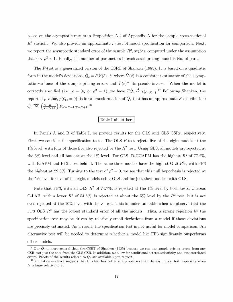
based on the asymptotic results in Proposition A.4 of Appendix A for the sample cross-sectional

R2 statistic. We also provide an approximate F -test of model specification for comparison. Next,

we report the asymptotic standard error of the sample R2, se(ρ2), computed under the assumption

that 0 < ρ2 < 1. Finally, the number of parameters in each asset pricing model is No. of para.

The F -test is a generalized version of the CSRT of Shanken (1985). It is based on a quadratic

form in the model’s deviations, Qc = e′V (e)+e, where V (e) is a consistent estimator of the asymp-

totic variance of the sample pricing errors and V (e)+ its pseudo-inverse. When the model is

correctly specified (i.e., e = 0N or ρ2 = 1), we have TQcA∼ χ2

N−K−1.17 Following Shanken, the

reported p-value, p(Qc = 0), is for a transformation of Qc that has an approximate F distribution:

Qcapp.∼

(

N−K−1T−N+1

)

FN−K−1,T−N+1.18

Table I about here

In Panels A and B of Table I, we provide results for the OLS and GLS CSRs, respectively.

First, we consider the specification tests. The OLS F -test rejects five of the eight models at the

1% level, with four of those five also rejected by the R2 test. Using GLS, all models are rejected at

the 5% level and all but one at the 1% level. For OLS, D-CCAPM has the highest R2 of 77.2%,

with ICAPM and FF3 close behind. The same three models have the highest GLS R2s, with FF3

the highest at 29.8%. Turning to the test of ρ2 = 0, we see that this null hypothesis is rejected at

the 5% level for five of the eight models using OLS and for just three models with GLS.

Note that FF3, with an OLS R2 of 74.7%, is rejected at the 1% level by both tests, whereas

C-LAB, with a lower R2 of 54.8%, is rejected at about the 5% level by the R2 test, but is not

even rejected at the 10% level with the F -test. This is understandable when we observe that the

FF3 OLS R2 has the lowest standard error of all the models. Thus, a strong rejection by the

specification test may be driven by relatively small deviations from a model if those deviations

are precisely estimated. As a result, the specification test is not useful for model comparison. An

alternative test will be needed to determine whether a model like FF3 significantly outperforms

other models.

17Our Qc is more general than the CSRT of Shanken (1985) because we can use sample pricing errors from anyCSR, not just the ones from the GLS CSR. In addition, we allow for conditional heteroskedasticity and autocorrelatederrors. Proofs of the results related to Qc are available upon request.

18Simulation evidence suggests that this test has better size properties than the asymptotic test, especially whenN is large relative to T .

17

Another issue is the number of factors in a model. While ICAPM has five factors, the other

models considered have at most three factors. The extra degrees of freedom will be an advantage

for ICAPM in any given sample, holding true explanatory power constant across models. However,

our formal test will take this sampling variation into account and enable us to infer whether the

model is superior in population, i.e., whether it better explains true expected returns.

Assuming that 0 < ρ2 < 1, se(ρ2) captures the sampling variability of ρ2. In Table I, we

observe that the ρ2s of several models are quite volatile. In particular, the ICAPM GLS R2 is not

significantly different from zero; despite being the second highest of eight R2s, its standard error

is the largest. Four of the eight OLS standard errors exceed 0.2, with U-CCAPM’s the highest at

0.244. This high volatility will make it hard to distinguish between models.19

Several observations emerge from the results in Table I. First, there is strong evidence of the need

to incorporate model misspecification into our statistical analysis. Second, there is considerable

sampling variability in ρ2 and so it is not entirely clear whether one model truly outperforms the

others. Finally, specification-test results are sometimes sensitive to whether we employ OLS or

GLS estimation, and it is not always the case that models with high ρ2s pass the specification test.

B.2. Properties of the γ and λ Estimates under Correctly Specified and PotentiallyMisspecified Models

Next, we examine the pricing results based on the γ and λ estimators. As far as we know, all

previous CSR studies except the recent paper by Shanken and Zhou (2007) have used standard

errors that assume the model is correctly specified. As we argued in the introduction, it is difficult

to justify this practice because (as we just saw empirically) some, if not all, of the models are bound

to be misspecified. In this subsection, we investigate whether inferences about pricing are affected

by using an asymptotic standard error that is robust to such model misspecification.

In Table II, we focus on the zero-beta rate and risk premium estimates, γ, of the beta pricing

models. For each model, we report γ and associated t-ratios under correctly specified and potentially

misspecified models. For correctly specified models, we give the t-ratio of Fama and MacBeth

19With a one-lag Newey-West adjustment, the p-values under 0.10 for the R2-based specification test barely change(OLS and GLS). For the F -test, the only noteworthy change is a decline in the OLS D-CCAPM p-value from 0.077to 0.037. P -values for the OLS and GLS tests of ρ2 = 0 hardly change. Finally, most of the standard errors of ρ2

barely change. The largest change across all specifications is an increase for U-CCAPM from 0.244 to 0.269 (OLS).

18

(1973), followed by that of Shanken (1992) and Jagannathan and Wang (1998), which account for

estimation error in the betas. Last, is the t-ratio under a potentially misspecified model, based on

our new results provided in Appendix A. The various t-ratios are identified by subscripts fm, s,

jw, and pm, respectively.

Table II about here

We see evidence in Panel A (OLS) that the ultimate consumption factor cg36, the value-growth

factor hml and the prem state variable have coefficients that are reliably positive at the 5% level.

In Panel B (GLS), hml is again positively priced. As in many past studies, the market factor

vw is negatively priced in several specifications, contrary to the usual theoretical prediction.20 In

addition, the zero-beta rates exceed the risk-free rate (the average one-month T-bill rate was 0.45%

per month) by large amounts that would seem hard to reconcile with theory. We return to these

issues later on.

Consistent with our theoretical results, we find that the t-ratios under correctly specified and

potentially misspecified models are similar for traded factors, e.g., the FF3 factors, but they can

differ substantially for factors that have low correlations with asset returns. As an example of the

latter, consider the consumption factor cg in D-CCAPM. With GLS estimation, we have t-ratiofm =

2.50, t-ratios = 2.20, t-ratiojw = 2.14, and t-ratiopm = 1.36, which shows that the misspecification

adjustment can make a significant difference. ICAPM provides another illustration of the different

conclusions that one can reach by using misspecification-robust standard errors. While the t-ratios

under correctly specified models in Panel B suggest that γterm is highly statistically significant

(t-ratiofm = 3.07, t-ratios = 2.58, and t-ratiojw = 2.59), the robust t-ratio is only 1.61, not quite

significant at the 10% level. The scale factor cay is one more example. In short, both model

misspecification and beta estimation error materially affect inference about the expected return

relation.

As discussed in Section II.A, there are issues with testing whether an individual factor risk

premium is zero or not in a multi-factor model. Unless the factors are uncorrelated, only the prices

of covariance risk (elements of λ1) allow us to identify factors that improve the explanatory power

20The market premium is positive in CAPM. In ICAPM, it is positive after controlling for the market’s exposureto the hedging factors. See, for example, Fama (1996).

19

of the expected return model (equivalently, simple regression betas can be used). The usual risk

premium for a given factor does not permit such an inference. Table III presents estimation results

for λ. To conserve space, only the OLS t-ratios under potentially misspecified models are presented.

Table III about here

As an illustration of our point that risk premia and prices of covariance risk can deliver different

messages, consider FF3. The size-factor coefficient λsmb is statistically significant at the 1% level,

with a robust t-ratio of 2.79. In contrast, γsmb in Table II has a robust t-ratio of only 1.19. The

reverse occurs for the value-growth factor, with λhml not quite significant at the 10% level, yet

γhml commanding a t-ratio of 3.42 earlier. Hence, by focusing on the usual risk premia (the γs),

one might think that smb is not an important factor in FF3 and that hml is. This conclusion

would be incorrect, however. Results for the prices of covariance risk (the λs) imply that smb has

explanatory power for the cross-section of expected returns above and beyond the other factors in

FF3, while the role of hml is questionable. Thus, surprisingly, we cannot reject the hypothesis that

the expected returns generated by a two-factor model consisting of the market and smb equal those

based on FF3.21

To summarize, accounting for model misspecification often makes a qualitative difference in

determining whether estimates of the risk premia or the prices of covariance risk are statistically

significant, especially when the factor has low correlation with asset returns. This is the case

for several of the models (ICAPM, D-CCAPM, CC-CAY) that include macroeconomic or scaled

factors. In addition, we have seen that focusing on the γs, rather than λs, as is typical in the

literature, can lead to erroneous conclusions as to whether a factor is helpful in explaining the

cross-section of expected returns.22

B.3. Tests of Equality of the Cross-Sectional R2s of Two Competing Models

In Table IV, we report pairwise tests of equality of R2s for different models, some nested and

others non-nested. For the reasons discussed earlier, we present the normal test for non-nested

21As expected, for one-factor models, γ1 and λ1 result in similar inferences. In this case, the t-ratios of the γ1 andλ1 would be identical if we imposed the null hypotheses of γ1 = 0 and λ1 = 0, so that the EIV adjustment termsdrop out of the analysis.

22Most of the changes in t-statistics with a one-lag Newey-West adjustment are trivial, with the largest across allspecifications being a drop from 2.34 to 2.10 for the OLS estimator γcg36.

20

models and comment briefly on the sequential test results. Panel A is for the OLS CSR and

Panel B is for the GLS CSR. Each panel shows the differences between the sample cross-sectional

R2s for various pairs of models and the associated p-values (in parentheses). In the case of non-

nested models, the reported p-values are two-tailed p-values. We use boldface to highlight those

cases in which the p-value is at most 0.05.

Table IV about here

The main findings can be summarized as follows. First, the results show that CAPM and

CCAPM are often outperformed by other models at the 1% and 5% levels. Specifically, CCAPM is

dominated at the 5% level by U-CCAPM, FF3, D-CCAPM and ICAPM in Panel A, and again by

the last two models in Panel B. CAPM is dominated by C-LAB, FF3 and D-CCAPM in Panel A,

and by FF3 in Panel B. In many cases the OLS R2 differences with CAPM exceed 60 or 70

percentage points. In addition, FF3 dominates the consumption models CC-CAY (OLS and GLS)

and U-CCAPM (GLS).23

There are several cases of large R2 differences that do not give rise to statistical rejections due

to limited precision of the estimates. Recall, for example, that U-CCAPM has the highest OLS

standard error (0.244) in Table I. Despite an R2 difference of 27 percentage points in favor of FF3,

the p-value in Panel A of Table IV is 0.226. As another example, the ICAPM OLS R2 exceeds

that of CAPM by a full 65 percentage points and still just misses being statistically significant at

the 5% level. Clearly, the common practice of simply comparing sample R2 values is not a reliable

method for identifying superior models.24

We have also explored the effect of including the three Fama-French factors, along with the 30

portfolios, as test assets in the various model comparisons. For models with one or more of these

traded factors, inclusion requires that the estimated price of risk conform to the corresponding

model restriction (i.e., equal the expected market premium over the zero-beta rate or equal the

expected spread return for smb and hml). As discussed by Lewellen, Nagel and Shanken (2010),

this holds either exactly (GLS) or approximately (OLS). The changes in results here are minimal,

23As noted earlier, all the p-values in Table IV are computed under the assumption that the relevant terms areserially uncorrelated. For p-values less than 0.10, the largest change observed with a one-lag Newey-West adjustmentis an increase from 0.032 to 0.049 for the CCAPM/U-CCAPM comparison. Most other changes are trivial.

24In one of nine cases, the sequential test no longer rejects at the 5% level.

21

perhaps because the factors are closely mimicked by the original test assets. For comparison with

other studies, we also performed the analysis using just the 25 size and book-to-market portfolios.

The range in R2s was slightly wider in this case and the standard error of ρ2 was higher for every

model. Consistent with the lower precision, there were 11 instances of model comparison rejections

at the 5% level, as compared to 15 in Table IV.

Inherent in model misspecification is the fact that one model may exhibit superior performance

with some test assets, but poorer performance with other assets. To explore this possibility, we

repeated the analysis with 25 portfolios formed by first sorting stocks into quintiles based on size

and then, within each size quintile, by the estimate of the simple vw beta.25 In contrast to the

earlier results, the performance of CC-CAY is impressive with these portfolios. Its OLS R2 is 0.874

(0.366 earlier), about the same as that for ICAPM, and CC-CAY actually dominates FF3 at the

5% level. With GLS estimation, its R2 of 0.432 is the highest of all the models and CC-CAY is the

only model not rejected by the specification tests. Thus, we see that model comparison can be very

sensitive to the test assets employed. However, the comparatively strong performance of ICAPM

is a fairly robust empirical finding for the test portfolios we have examined.

B.4. Excess Returns Analysis

Consistent with standard practice in the literature, the CSR analysis thus far has proceeded with

the zero-beta rate and risk premium coefficients unconstrained. The resulting R2 is a reasonable

measure of a model’s success in explaining cross-sectional differences in average returns. However,

given the high values of the zero-beta rate and the negative market premia, we may not want to

“credit” the theories for all of this explanatory power. One way of dealing with this issue is to

constrain the zero-beta rate to equal the risk-free rate, a practice that is common in other parts

of the empirical asset pricing literature. For example, studies that focus on time-series “alphas”

when all factors are traded impose this restriction (see, for example, Gibbons, Ross and Shanken

(1989)).

We implement the zero-beta rate restriction in the CSR context by working with test port-

folio returns in excess of the T-bill rate, while excluding the constant from the expected return

25All NYSE-AMEX-NASDAQ common stocks are considered. This is similar to the approach of Fama and French(1992). We use quintiles, rather than deciles, to mitigate potential finite-sample issues related to the inversion of alarge sample covariance matrix. The results of this analysis are available upon request.

22

relations.26 Thus, expected excess return is simply the sum of the betas times the corresponding

risk premia coefficients. As is typical for regression analysis without a constant, the corresponding

R2 measure involves (weighted) sums of squared values of the dependent variable (mean excess

returns) in the denominator, not squared deviations from the cross-sectional average. This ensures

that R2 is always between 0 and 1.

Table V presents R2s and other model information for the excess returns specification, in the

same format as Table I. The first thing that we notice are the large OLS values of R2. These

numbers are not directly comparable to the earlier values, however, for the reason just mentioned.

Since the models do not include a constant, simply getting the overall level of mean returns right

will now enhance a model’s R2. In contrast, a positive value of the earlier goodness-of-fit measure

indicates that a model has some ability to explain deviations of mean test-portfolio returns from

the cross-sectional average.

Table V about here

The OLS sample R2 measures in Panel A range from 0.858 (CAPM) to 0.972 (ICAPM), whereas

the GLS values in Panel B are much lower, ranging from 0.044 (CCAPM) to 0.339 (ICAPM).

Moreover, ICAPM is the only model that is not rejected at the 5% level by either OLS specification

test. For brevity, we do not report the detailed pricing results, but note that the market risk

premium estimates are now all positive with the constrained zero-beta rate. In addition, OLS γs

for cg (in CCAPM), cg36, vw, hml, and term are significantly positive, while those for rf and div

are significantly negative at the 5% level. The GLS results are similar, except that cg is no longer

significant.

The D-CCAPM factor cgdur is no longer significantly priced using excess returns, and the

model, which was the top OLS performer earlier, now has one of the lowest cross-sectional R2

values. Thus, although a linear function of the D-CCAPM betas came closest to spanning expected

returns earlier (in the OLS metric), it did so with a zero-beta rate almost two percentage points

per month above the risk-free rate. With that coefficient constrained to equal the T-bill rate, the

26With the zero-beta rate constrained in this manner, it follows from the results of Kan and Robotti (2008) thatequality of GLS R2s for two models is equivalent to equality of their HJ-distances, provided that the SDF is writtenas a linear function of the de-meaned factors. No such relation exists for the OLS R2. The details of the excessreturns analysis are provided in Appendix D.

23

fit of the model deteriorates substantially. On the other hand, U-CCAPM moves up in the OLS

rankings, now just behind ICAPM and FF3. Also noteworthy is the fact that hml is the dominant

factor in this FF3 specification, i.e., it now has a significant price of covariance risk, while smb does

not.

To conserve space, we simply summarize the model comparison results. There are fewer rejec-

tions now. FF3 dominates CAPM (OLS and GLS), CCAPM and D-CCAPM (both GLS), all at

the 1% level. There are no additional rejections at the 5% level, although FF3 barely misses over

C-LAB (GLS) and ICAPM comes close to dominating CAPM (OLS and GLS). It is interesting

to note that while FF3 dominates more models statistically, ICAPM has the higher sample R2s.

Precision appears to play a role in this. The standard error of ICAPM’s GLS R2 is the highest of

all the models. Again, the importance of taking into account information about sampling variation

is evident.27

Earlier, we noted that the performance of CC-CAY was impressive with size-beta portfolios

employed as the test assets. The model even dominated FF3 at the 5% level (OLS). This is no

longer true in the excess returns specification with size-beta portfolios. In this case, ICAPM is again

the top OLS performer, followed by FF3. However, CAPM is the only model dominated at the 5%

level. With GLS estimation, the CC-CAY R2 of 0.5 is about twice that of the nearest competitor,

but due to its large standard error (0.196), the model does not dominate FF3 or ICAPM, even at

the 10% level.

In short, with the zero-beta rate constrained to equal the risk-free rate, only ICAPM and FF3

consistently rank at or near the top of our list of models based on the cross-sectional R2. However,

apart from CAPM and CCAPM, only D-CCAPM is ever dominated at the 5% level.

IV. Multiple Model Comparison

Thus far, we have considered comparison of two competing models. However, given a set of

models of interest, one may want to test whether one model, the “benchmark,” has the highest ρ2

of all models in the set. This gives rise to a common problem in applied work — if we focus on the

statistic that provides the strongest evidence of rejection, without taking into account the process

27The sequential test delivers the same conclusions as the normal test at the 5% level.

24

of searching across alternative specifications, there will be a tendency to reject the benchmark more

often than the nominal size of the tests suggests.28 In other words, the true p-value will be larger

than the one associated with the most extreme statistic. For example, in a head-on competition,

we saw earlier that FF3 dominates C-LAB at the 5% level with GLS estimation. But will C-LAB

still be statistically rejected from the perspective of multiple model comparison?

In this section, we develop and implement a formal test of multiple model comparison. This

is a multivariate inequality test based on results in the statistics literature due to Wolak (1987,

1989). Suppose we have p models. Let ρ2i denote the population cross-sectional R2 of model i and

let δ ≡ (δ2, . . . , δp), where δi ≡ ρ21 − ρ2

i . We are interested in testing the null hypothesis that the

benchmark, model 1, performs at least as well as all others, i.e., H0 : δ ≥ 0r with r = p − 1. The

alternative is that some model has a higher population R2 than model 1.

The test is based on the sample counterpart of δ, δ ≡ (δ2, . . . , δp), where δi ≡ ρ21 − ρ2

i . We

assume that 0 < ρ2i < 1 for all i, so that δ has an asymptotic normal distribution with mean δ and

covariance matrix Σδ

(additional technical conditions are provided in Appendix E).

Let δ be the optimal solution in the following quadratic programming problem:

minδ

(δ − δ)′Σ−1

δ(δ − δ) s.t. δ ≥ 0r, (13)

where Σδ

is a consistent estimator of Σδ. The likelihood ratio test of the null hypothesis is

LR = T (δ − δ)′Σ−1

δ(δ − δ). (14)

Since the null hypothesis is composite, to construct a test with the desired size, we require the

distribution of LR under the least favorable value of δ, which is δ = 0r. This distribution is derived

in Appendix E, along with a numerically efficient computational procedure that greatly improves

on methods employed in previous research. We use this procedure to obtain asymptotically valid

p-values.

In comparing a benchmark model with a set of alternative models, we first remove those al-

ternative models i that are nested by the benchmark model since, by construction, δi ≥ 0 in this

case. If any of the remaining alternatives is nested by another alternative model, we remove the

28Chen and Ludvigson (2009) employ the “reality check” of White (2000) to draw inferences about multiple modelcomparison with the HJ-distance.

25

“smaller” model since the ρ2 of the “larger” model will be at least as big. Finally, we also remove

from consideration any alternative models that nest the benchmark, since the normality assumption

on δi does not hold under the null hypothesis that δi = 0. An alternative testing procedure for

multiple model comparison is needed in this case. We return to this issue below. Table VI provides

our findings.

Table VI about here

For the OLS comparisons in Panel A, only CCAPM is rejected, with p-value 0.000. The GLS

results in Panel B provide additional evidence against the consumption models. CCAPM and CC-

CAY are rejected at the 5% level and U-CCAPM just misses rejection with p-value 0.053. C-LAB

which, as mentioned above, was dominated in the pairwise comparison with FF3 (p-value 0.025),

is no longer rejected in the multiple model comparison. The GLS p-value of 0.073 in Table VI is

higher than before, since it takes into account the element of searching over alternative models.

Next, we turn to the topic of nested multiple model comparison. Although the LR test is

no longer applicable here (δ is not asymptotically normally distributed), fortunately our earlier

approach to testing for equality of R2s can easily be adapted to this context. One need only

consider a single expanded model that includes all of the factors contained in the models that

nest the benchmark. For example, in the case of CCAPM, this expanded model includes cg, cay,

cay · cg, vw, and cgdur from CC-CAY and D-CCAPM. Using Lemma A.3 of Appendix A, it is

easily demonstrated that the expanded model dominates the benchmark model if and only if one

or more of the “larger” models dominate it. Thus, the null hypothesis that the benchmark model

has the same R2 as these alternatives can be tested using the earlier methodology.29

The results are as follows. The CCAPM p-values are 0.009 (OLS) and 0.092 (GLS), while the p-

values for CAPM are 0.057 (OLS) and 0.458 (GLS). Given the p-value of 0.001 for the CAPM/FF3

comparison in Table IV (OLS and GLS), a Bonferroni approach would have yielded a stronger

rejection of CAPM in this case. With four models nesting CAPM, the Bonferroni (upper-bound)

p-value is 4 × 0.001 = 0.004. But of course, the decision about which joint test to perform should

29If one of the models has a higher R2, then so will the expanded model. Conversely, if none of the models improvesthe R2, then for each of the additional factors, the vector of asset covariances must be orthogonal to the CSR residualsof the benchmark model, as will any linear combination of these covariance vectors. Thus, the expanded model musthave the same R2 as the benchmark.

26

really be made a priori.

We conclude with a few observations about results for our alternative empirical specifications.

Consistent with our earlier evidence that the performance of D-CCAPM declines in the excess

returns specification, the model is rejected at the 5% level in multiple comparison tests with excess

returns, as is CCAPM (GLS). Also, multiple model comparison confirms the decline of FF3 when

size-beta portfolios are employed. FF3 is rejected at the 5% level in this case, as are CAPM and

CCAPM (OLS). Since several models with lower R2s are not rejected, again the greater precision

with which the FF3 R2 is estimated contributes to this finding. With excess returns and size-beta

portfolios, however, only CAPM (OLS and GLS) and CCAPM (GLS) are dominated at the 5%

level.

V. Simulation Evidence

In this section, we explore the small-sample properties of our various test statistics via Monte

Carlo simulations. In all simulation experiments, the test assets are the 25 size and book-to-market

portfolios plus five industry portfolios used in most of our analysis. The time-series sample size is

taken to be T = 600, close to the actual sample size of 582 in our empirical work. The factors and

the returns on the test assets are drawn from a multivariate normal distribution. Both OLS and

GLS specifications are examined. We compare actual rejection rates over 10,000 iterations to the

nominal 5% level of our tests. A more detailed description of the various simulation designs can be

found in Appendix F.

We start with the specification tests — the R2 test based on Proposition A.4 of Appendix A

and the approximate F -test. To evaluate the size properties of these tests, we simulate data for a

world in which FF3 is exactly true with expected returns taken to be the sample estimates implied

by the model. The F -test of FF3 performs very well in both cases, with just a slight tendency to

over-reject (5.5% OLS, 5.6% GLS). The R2 test is right on the money for OLS, but rejects a bit too

much (7.8%) for GLS. To analyze the power of these tests, we simulate data assuming that expected

returns equal the sample means. This ensures that FF3 is now misspecified, with population R2s

in the simulations equal to the sample values observed earlier, 0.747 (OLS) and 0.298 (GLS). The

27

rejection rates for the specification tests of FF3 are close to one in all cases.30

Both of our tests of the hypothesis ρ2 = 0 have the correct size when we simulate a world in

which FF3 has no explanatory power, i.e., with expected returns taken to be orthogonal to the

FF3 loadings. The tests also display good power against alternatives where the true R2s for the

simulated data equal the sample R2s for FF3. Similar conclusions hold for the nested-models test

of equality of R2s, with CAPM nested in FF3. Here, the size of the test is inferred from simulations

in which CAPM is misspecified and the additional FF3 factors are of no help. Power for the nested-

models test is evaluated by simulating data for which the true R2s equal the sample values and

thus CAPM is dominated by FF3.

Next, we turn to our main test, the normal test of equality of R2s for non-nested models. In

this experiment, the expected returns are specified in such a way that ρ2 is the same for FF3 and

C-LAB, 0.647 (OLS) or 0.203 (GLS). These are averages of the sample R2s obtained earlier for the

two models. The size property of the test is very good in the OLS case (5.8%), while there is a

tendency to under-reject a bit (2.7%) with GLS (this tendency is more pronounced for lower values

of T ).

The power of the normal test is explored using the sample R2s of FF3 and C-LAB as the

population R2 values. These are 0.747 and 0.548 for OLS, 0.298 and 0.109 for GLS, so the null

hypothesis of equivalent model performance is false in these simulations. The rejection rate is only

14.6% for OLS, but somewhat higher at 31.5% in the GLS case. This is a reflection of the limited

precision of the sample R2s, given the substantial noise (unexpected) component of returns. We

also examined power using CCAPM and FF3 as the two models, with the CCAPM ρ2 equal to

0.044 (OLS) or 0.011 (GLS). Naturally, power increases substantially, given the large differences in

performance. The rejection rates are now 87% (OLS) and 76% (GLS).

Finally, we examine the multiple-comparison inequality test for non-nested models. Recall that

the composite null hypothesis for this test maintains that ρ2 for the benchmark model is at least as

high as that for all other models under consideration. Therefore, to evaluate size, we consider the

case in which all models have the same ρ2 value, so as to maximize the likelihood of rejection under

the null. We simulate six different single-factor models corresponding to the factors vw, smb, cg36,

30When the nominal size of the test differs from the actual size, this should be interpreted as power correspondingto the latter.

28

lab, prem, and rf and implement the likelihood ratio test with r = 5. The rejection rates range

from 3.3% to 5% (OLS) and from 2.7% to 6% (GLS). Thus, the tests are fairly well specified under

the null of equivalent model performance.

To examine power, we simulate five of our original models, CCAPM, U-CCAPM, C-LAB,

FF3, and ICAPM, with the earlier sample R2s serving as the population R2s. Since FF3 and

ICAPM have the highest R2s, we let each of the remaining models serve as the null model in

a multiple comparison test against four alternative models. Thus, we evaluate power for three

different scenarios: the rejection rates for the OLS test are 13.8% (C-LAB), 35.9% (U-CCAPM),

and 86.3% (CCAPM). The corresponding GLS numbers are 25.1%, 64.9%, and 72%, respectively.

Naturally, power increases as the ρ2 of the benchmark model decreases, and “good” power requires

that the differences in model performance are fairly large.

Overall, these simulation results suggest that the tests should be fairly reliable for the sample

size encountered in our empirical work.

VI. Conclusion

We have provided an analysis of the asymptotic properties of the traditional cross-sectional

regression methodology and the associated R2 goodness-of-fit measure when an underlying beta

pricing model fails to hold exactly. The importance of adjusting standard errors for model misspec-

ification has also been demonstrated empirically for several prominent asset pricing models. As far

as we know, our study is the first to consider (analytically or even in simulations) the important

sampling distribution of the difference between the sample R2s of two competing models. As we

show, the asymptotic distribution of this difference depends on whether the models are correctly

specified and whether they are nested or non-nested.

Our main analysis employs the 25 Fama-French size and book-to-market portfolios plus five

industry portfolios as the test assets. In this case, the ICAPM specification of Petkova (2006) is the

best overall performer, with the three-factor model of Fama and French (FF3, 1993) right behind.

The R2 differences for comparing these two models are not reliably different from zero, however,

whether OLS or GLS estimation is employed, and whether the zero-beta rate is constrained to equal

the risk-free rate or not. The durable goods consumption model of Yogo (2006) is competitive with

29

FF3 and ICAPM in the main analysis, but its performance declines dramatically when we impose

economic restrictions on the zero-beta rates.

With an alternative set of test assets, 25 size-beta portfolios, some important changes emerge.

The conditional CCAPM of Lettau and Ludvigson (2001), one of the poorer performers in the main

analysis, now competes with ICAPM for top honors in several specifications. On the other hand,

FF3 exhibits some vulnerability with these test assets, and is dominated at the 5% level by both

models.

The evidence discussed above involves pairwise model comparison. While these methods take us

well beyond the common practice of simply comparing point estimates of R2, those tests are open to

a criticism common in applied work, i.e., that the process of searching over various models to identify

interesting results can lead to an overstatement of statistical significance. We address this issue

by introducing tests of multiple model comparison for nested and non-nested models. Naturally,

this results in fewer rejections than were obtained earlier. Several of our main conclusions are

reinforced, however: rejections of the basic CAPM and CCAPM, near-rejections (at the 5% level)

of both the conditional and ultimate CCAPMs, rejection of the durable CCAPM in the excess

returns specification, and rejection of FF3 when the test assets are size-beta portfolios.

To sum up, the robust performance of ICAPM and the fact that it is the only model that is

never statistically dominated in any of our analyses is impressive. Nevertheless, we should keep in

mind that the ICAPM R2 is sometimes not estimated very precisely. Also, the model achieves its

superior explanatory power with five factors, two more than any of the competing models. Still,

while this undoubtedly can be an advantage, additional risk measures certainly do not have to be

related to actual expected returns, and our statistical analysis does take into account sampling

variation related to the larger degrees of freedom.

Looking to the future, other asset pricing models not considered here could, of course, be

examined. In terms of the methodology, although our simulation results are encouraging, the

small-sample properties of the test statistics proposed in this paper should be explored further.

Other metrics for comparing models besides the cross-sectional R2 could also be considered. Finally,

incorporating theoretical restrictions on the risk premia in the measure of model performance might

be a way of enhancing power and providing more informative model comparison tests.

30

References

Black, Fischer, Michael C. Jensen, and Myron Scholes, 1972, The capital asset pricing model:

Some empirical tests, in Michael C. Jensen, ed.: Studies in the Theory of Capital Markets

(Praeger, New York).

Campbell, John Y., 1996, Understanding risk and return, Journal of Political Economy 104, 298–

345.

Chen, Nai-Fu, Richard Roll, and Stephen A. Ross, 1986, Economic forces and the stock market,

Journal of Business 59, 383–404.

Chen, Xiaohong, and Sydney C. Ludvigson, 2009, Land of addicts? An empirical investigation of

habit-based asset pricing models, Journal of Applied Econometrics 24, 1057–1093.

Cochrane, John H., 1996, A cross-sectional test of an investment-based asset pricing model, Jour-

nal of Political Economy 104, 572–621.

Cochrane, John H., 2005. Asset Pricing (Princeton University Press, Princeton).

Fama, Eugene F., 1996, Multifactor portfolio efficiency and multifactor asset pricing, Journal of

Financial and Quantitative Analysis 3, 441–465.

Fama, Eugene F., and James D. MacBeth, 1973, Risk, return, and equilibrium: Empirical tests,

Journal of Political Economy 71, 607–636.

Fama, Eugene. F., and Kenneth R. French, 1992, The cross-section of expected stock returns,

Journal of Finance 47, 427–466.

Fama, Eugene. F., and Kenneth R. French, 1993, Common risk factors in the returns on stocks

and bonds, Journal of Financial Economics 33, 3–56.

Gibbons, Michael R., Stephen A. Ross, and Jay Shanken, 1989, A test of the efficiency of a given

portfolio, Econometrica 57, 1121–1152.

Golden, Richard M., 2003, Discrepancy risk model selection test theory for comparing possibly

misspecified or nonnested models, Psychometrika 68, 229–249.

31

Hall, Alastair R., and Atsushi Inoue, 2003, The large sample behaviour of the generalized method

of moments estimator in misspecified models, Journal of Econometrics 114, 361–394.

Hansen, Lars P., 1982, Large sample properties of generalized method of moments estimators,

Econometrica 50, 1029–1054.

Hansen, Lars P., and Ravi Jagannathan, 1997, Assessing specification errors in stochastic discount

factor models, Journal of Finance 52, 557–590.

Hou, Kewei, and Robert Kimmel, 2006, On the estimation of risk premia in linear factor models,

Working paper, Ohio State University.

Jagannathan, Ravi, and Zhenyu Wang, 1996, The conditional CAPM and the cross-section of

expected returns, Journal of Finance 51, 3–53.

Jagannathan, Ravi, and Zhenyu Wang, 1998, An asymptotic theory for estimating beta-pricing

models using cross-sectional regression, Journal of Finance 53, 1285–1309.

Jagannathan, Ravi, Keiichi Kubota, and Hitoshi Takehara, 1998, Relationship between labor-

income risk and average return: Empirical evidence from the Japanese stock market, Journal

of Business 71, 319–348.

Jagannathan, Ravi, and Yong Wang, 2007, Lazy investors, discretionary consumption, and the

cross-section of stock returns, Journal of Finance 62, 1623–1661.

Jagannathan, Ravi, Georgios Skoulakis, and Zhenyu Wang, 2010, The analysis of the cross-section

of security returns, in Yacine Ait-Sahalia and Lars Hansen, eds.: Handbook of Financial

Econometrics (Elsevier, Amsterdam).

Jørgensen–Vissing, Annette, and Orazio P. Attanasio, 2003, Stock-market participation, intertem-

poral substitution, and risk-aversion, American Economic Review Papers and Proceedings 93,

383–391.

Kan, Raymond, and Cesare Robotti, 2008, Specification tests of asset pricing models using excess

returns, Journal of Empirical Finance 15, 816–838.

Kan, Raymond, and Cesare Robotti, 2009, Model comparison using the Hansen-Jagannathan

distance, Review of Financial Studies 22, 3449–3490.

32

Kan, Raymond, and Cesare Robotti, 2011, On the estimation of asset pricing models using uni-

variate betas, Economics Letters 110, 117–121.

Kan, Raymond, and Chu Zhang, 1999, Two-pass tests of asset pricing models with useless factors,

Journal of Finance 54, 203–235.

Kan, Raymond, and Guofu Zhou, 2004, Hansen-Jagannathan distance: Geometry and exact dis-

tribution, Working paper, University of Toronto.

Kandel, Shmuel, and Robert F. Stambaugh, 1995, Portfolio inefficiency and the cross-section of

expected returns, Journal of Finance 50, 157–184.

Lettau, Martin, and Sydney C. Ludvigson, 2001, Resurrecting the (C)CAPM: A cross-sectional

test when risk premia are time-varying, Journal of Political Economy 109, 1238–1287.

Lewellen, Jonathan W., Stefan Nagel, and Jay Shanken, 2010, A skeptical appraisal of asset-pricing

tests, Journal of Financial Economics 96, 175–194.

Li, Haitao, Yuewu Xu, and Xiaoyan Zhang, 2010, Evaluating asset pricing models using the second

Hansen-Jagannathan distance, Journal of Financial Economics 97, 279–301.

Merton, Robert C., 1973, An intertemporal capital asset pricing model, Econometrica 41, 867–887.

Newey, Whitney K., and Kenneth D. West, 1987, A simple, positive semi-definite, heteroskedas-

ticity and autocorrelation consistent covariance matrix, Econometrica 55, 703–708.

Parker, Jonathan A., and Christian Julliard, 2005, Consumption risk and the cross-section of

expected returns, Journal Political Economy 113, 185–222.

Petkova, Ralitsa, 2006, Do the Fama-French factors proxy for innovations in predictive variables?,

Journal of Finance 61, 581–612.

Rivers, Douglas, and Quang H. Vuong, 2002, Model selection tests for nonlinear dynamic models,

Econometrics Journal 5, 1–39.

Roll, Richard, and Stephen A. Ross, 1994, On the cross-sectional relation between expected returns

and betas, Journal of Finance 49, 101–121.

33

Shanken, Jay, 1985, Multivariate tests of the zero-beta CAPM, Journal of Financial Economics

14, 327–348.

Shanken, Jay, 1990, Intertemporal asset pricing: An empirical investigation, Journal of Econo-

metrics 45, 99–120.

Shanken, Jay, 1992, On the estimation of beta-pricing models, Review of Financial Studies 5,

1–33.

Shanken, Jay, and Guofu Zhou, 2007, Estimating and testing beta pricing models: Alternative

methods and their performance in simulations, Journal of Financial Economics 84, 40–86.

Vuong, Quang H., 1989, Likelihood ratio tests for model selection and non-nested hypotheses,

Econometrica 57, 307–333.

White, Halbert L., 1994. Estimation, Inference and Specification Analysis (Cambridge University

Press, New York).

White, Halbert L., 2000, A reality check for data snooping, Econometrica 68, 1097–1127.

Wolak, Frank A., 1987, An exact test for multiple inequality and equality constraints in the linear

regression model, Journal of the American Statistical Association 82, 782–793.

Wolak, Frank A., 1989, Testing inequality constraints in linear econometric models, Journal of

Econometrics 31, 205–235.

Yogo, Motohiro, 2006, A consumption-based explanation of expected stock returns, Journal of

Finance 61, 539–580.

34

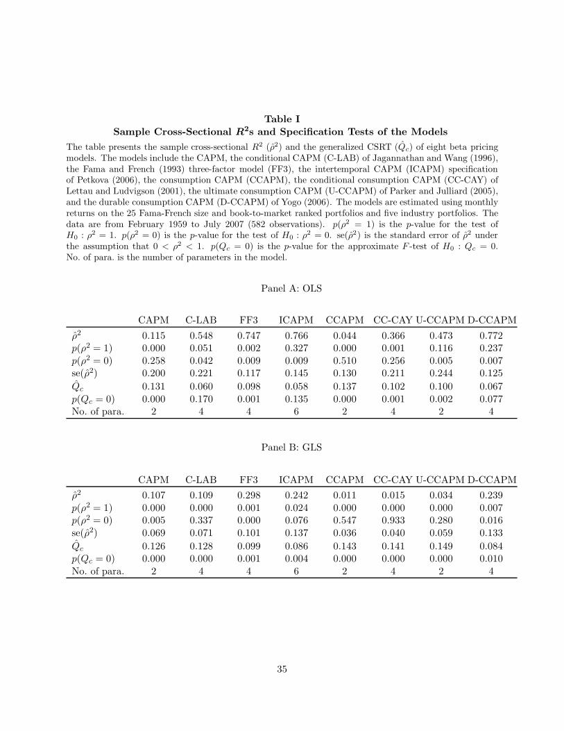
Table I

Sample Cross-Sectional R2s and Specification Tests of the Models

The table presents the sample cross-sectional R2 (ρ2) and the generalized CSRT (Qc) of eight beta pricingmodels. The models include the CAPM, the conditional CAPM (C-LAB) of Jagannathan and Wang (1996),the Fama and French (1993) three-factor model (FF3), the intertemporal CAPM (ICAPM) specificationof Petkova (2006), the consumption CAPM (CCAPM), the conditional consumption CAPM (CC-CAY) ofLettau and Ludvigson (2001), the ultimate consumption CAPM (U-CCAPM) of Parker and Julliard (2005),and the durable consumption CAPM (D-CCAPM) of Yogo (2006). The models are estimated using monthlyreturns on the 25 Fama-French size and book-to-market ranked portfolios and five industry portfolios. Thedata are from February 1959 to July 2007 (582 observations). p(ρ2 = 1) is the p-value for the test ofH0 : ρ2 = 1. p(ρ2 = 0) is the p-value for the test of H0 : ρ2 = 0. se(ρ2) is the standard error of ρ2 underthe assumption that 0 < ρ2 < 1. p(Qc = 0) is the p-value for the approximate F -test of H0 : Qc = 0.No. of para. is the number of parameters in the model.

Panel A: OLS

CAPM C-LAB FF3 ICAPM CCAPM CC-CAY U-CCAPM D-CCAPM

ρ2 0.115 0.548 0.747 0.766 0.044 0.366 0.473 0.772p(ρ2 = 1) 0.000 0.051 0.002 0.327 0.000 0.001 0.116 0.237

p(ρ2 = 0) 0.258 0.042 0.009 0.009 0.510 0.256 0.005 0.007se(ρ2) 0.200 0.221 0.117 0.145 0.130 0.211 0.244 0.125

Qc 0.131 0.060 0.098 0.058 0.137 0.102 0.100 0.067

p(Qc = 0) 0.000 0.170 0.001 0.135 0.000 0.001 0.002 0.077No. of para. 2 4 4 6 2 4 2 4

Panel B: GLS

CAPM C-LAB FF3 ICAPM CCAPM CC-CAY U-CCAPM D-CCAPM

ρ2 0.107 0.109 0.298 0.242 0.011 0.015 0.034 0.239

p(ρ2 = 1) 0.000 0.000 0.001 0.024 0.000 0.000 0.000 0.007p(ρ2 = 0) 0.005 0.337 0.000 0.076 0.547 0.933 0.280 0.016

se(ρ2) 0.069 0.071 0.101 0.137 0.036 0.040 0.059 0.133

Qc 0.126 0.128 0.099 0.086 0.143 0.141 0.149 0.084p(Qc = 0) 0.000 0.000 0.001 0.004 0.000 0.000 0.000 0.010

No. of para. 2 4 4 6 2 4 2 4

35

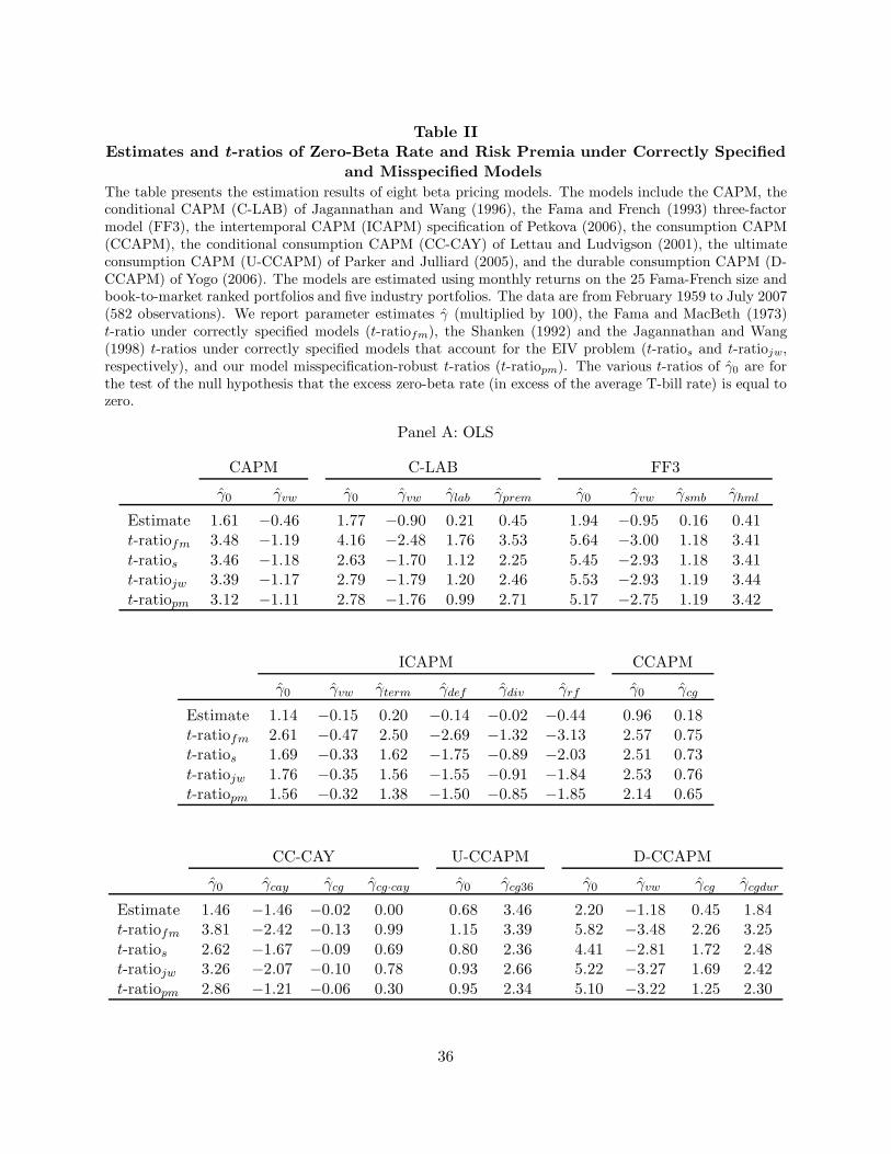
Table IIEstimates and t-ratios of Zero-Beta Rate and Risk Premia under Correctly Specified

and Misspecified Models

The table presents the estimation results of eight beta pricing models. The models include the CAPM, theconditional CAPM (C-LAB) of Jagannathan and Wang (1996), the Fama and French (1993) three-factormodel (FF3), the intertemporal CAPM (ICAPM) specification of Petkova (2006), the consumption CAPM(CCAPM), the conditional consumption CAPM (CC-CAY) of Lettau and Ludvigson (2001), the ultimateconsumption CAPM (U-CCAPM) of Parker and Julliard (2005), and the durable consumption CAPM (D-CCAPM) of Yogo (2006). The models are estimated using monthly returns on the 25 Fama-French size andbook-to-market ranked portfolios and five industry portfolios. The data are from February 1959 to July 2007(582 observations). We report parameter estimates γ (multiplied by 100), the Fama and MacBeth (1973)t-ratio under correctly specified models (t-ratiofm), the Shanken (1992) and the Jagannathan and Wang(1998) t-ratios under correctly specified models that account for the EIV problem (t-ratios and t-ratiojw,respectively), and our model misspecification-robust t-ratios (t-ratiopm). The various t-ratios of γ0 are forthe test of the null hypothesis that the excess zero-beta rate (in excess of the average T-bill rate) is equal tozero.

Panel A: OLS

CAPM C-LAB FF3

γ0 γvw γ0 γvw γlab γprem γ0 γvw γsmb γhml

Estimate 1.61 −0.46 1.77 −0.90 0.21 0.45 1.94 −0.95 0.16 0.41t-ratiofm 3.48 −1.19 4.16 −2.48 1.76 3.53 5.64 −3.00 1.18 3.41

t-ratios 3.46 −1.18 2.63 −1.70 1.12 2.25 5.45 −2.93 1.18 3.41t-ratiojw 3.39 −1.17 2.79 −1.79 1.20 2.46 5.53 −2.93 1.19 3.44

t-ratiopm 3.12 −1.11 2.78 −1.76 0.99 2.71 5.17 −2.75 1.19 3.42

ICAPM CCAPM

γ0 γvw γterm γdef γdiv γrf γ0 γcg

Estimate 1.14 −0.15 0.20 −0.14 −0.02 −0.44 0.96 0.18t-ratiofm 2.61 −0.47 2.50 −2.69 −1.32 −3.13 2.57 0.75t-ratios 1.69 −0.33 1.62 −1.75 −0.89 −2.03 2.51 0.73

t-ratiojw 1.76 −0.35 1.56 −1.55 −0.91 −1.84 2.53 0.76t-ratiopm 1.56 −0.32 1.38 −1.50 −0.85 −1.85 2.14 0.65

CC-CAY U-CCAPM D-CCAPM

γ0 γcay γcg γcg·cay γ0 γcg36 γ0 γvw γcg γcgdur

Estimate 1.46 −1.46 −0.02 0.00 0.68 3.46 2.20 −1.18 0.45 1.84t-ratiofm 3.81 −2.42 −0.13 0.99 1.15 3.39 5.82 −3.48 2.26 3.25

t-ratios 2.62 −1.67 −0.09 0.69 0.80 2.36 4.41 −2.81 1.72 2.48t-ratiojw 3.26 −2.07 −0.10 0.78 0.93 2.66 5.22 −3.27 1.69 2.42

t-ratiopm 2.86 −1.21 −0.06 0.30 0.95 2.34 5.10 −3.22 1.25 2.30

36

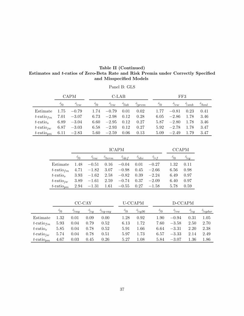
Table II (Continued)Estimates and t-ratios of Zero-Beta Rate and Risk Premia under Correctly Specified

and Misspecified Models

Panel B: GLS

CAPM C-LAB FF3

γ0 γvw γ0 γvw γlab γprem γ0 γvw γsmb γhml

Estimate 1.75 −0.79 1.74 −0.79 0.01 0.02 1.77 −0.81 0.23 0.41t-ratiofm 7.01 −3.07 6.73 −2.98 0.12 0.28 6.05 −2.86 1.78 3.46

t-ratios 6.89 −3.04 6.60 −2.95 0.12 0.27 5.87 −2.80 1.78 3.46t-ratiojw 6.87 −3.03 6.58 −2.93 0.12 0.27 5.92 −2.78 1.78 3.47

t-ratiopm 6.11 −2.83 5.60 −2.59 0.06 0.13 5.09 −2.49 1.79 3.47

ICAPM CCAPM

γ0 γvw γterm γdef γdiv γrf γ0 γcg

Estimate 1.48 −0.51 0.16 −0.04 0.01 −0.27 1.32 0.11

t-ratiofm 4.71 −1.82 3.07 −0.98 0.45 −2.66 6.56 0.98t-ratios 3.93 −1.62 2.58 −0.82 0.39 −2.24 6.49 0.97

t-ratiojw 3.89 −1.61 2.59 −0.74 0.37 −2.09 6.40 0.97t-ratiopm 2.94 −1.31 1.61 −0.55 0.27 −1.58 5.78 0.59

CC-CAY U-CCAPM D-CCAPM

γ0 γcay γcg γcg·cay γ0 γcg36 γ0 γvw γcg γcgdur

Estimate 1.32 0.01 0.09 0.00 1.28 0.92 1.90 −0.94 0.31 1.05t-ratiofm 5.93 0.04 0.79 0.52 6.13 1.72 7.60 −3.58 2.50 2.70

t-ratios 5.85 0.04 0.78 0.52 5.91 1.66 6.64 −3.31 2.20 2.38t-ratiojw 5.74 0.04 0.78 0.51 5.97 1.73 6.57 −3.33 2.14 2.49

t-ratiopm 4.67 0.03 0.45 0.26 5.27 1.08 5.84 −3.07 1.36 1.86

37

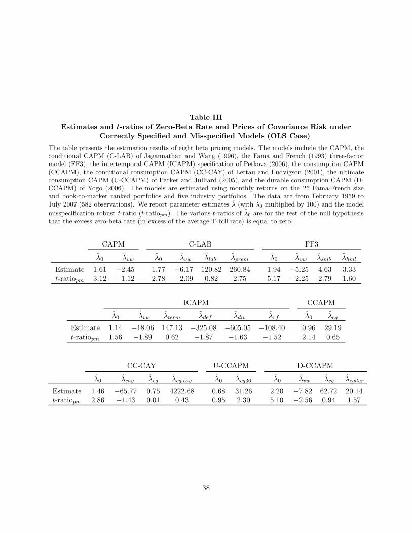
Table IIIEstimates and t-ratios of Zero-Beta Rate and Prices of Covariance Risk under

Correctly Specified and Misspecified Models (OLS Case)

The table presents the estimation results of eight beta pricing models. The models include the CAPM, theconditional CAPM (C-LAB) of Jagannathan and Wang (1996), the Fama and French (1993) three-factormodel (FF3), the intertemporal CAPM (ICAPM) specification of Petkova (2006), the consumption CAPM(CCAPM), the conditional consumption CAPM (CC-CAY) of Lettau and Ludvigson (2001), the ultimateconsumption CAPM (U-CCAPM) of Parker and Julliard (2005), and the durable consumption CAPM (D-CCAPM) of Yogo (2006). The models are estimated using monthly returns on the 25 Fama-French sizeand book-to-market ranked portfolios and five industry portfolios. The data are from February 1959 toJuly 2007 (582 observations). We report parameter estimates λ (with λ0 multiplied by 100) and the model

misspecification-robust t-ratio (t-ratiopm). The various t-ratios of λ0 are for the test of the null hypothesisthat the excess zero-beta rate (in excess of the average T-bill rate) is equal to zero.

CAPM C-LAB FF3

λ0 λvw λ0 λvw λlab λprem λ0 λvw λsmb λhml

Estimate 1.61 −2.45 1.77 −6.17 120.82 260.84 1.94 −5.25 4.63 3.33

t-ratiopm 3.12 −1.12 2.78 −2.09 0.82 2.75 5.17 −2.25 2.79 1.60

ICAPM CCAPM

λ0 λvw λterm λdef λdiv λrf λ0 λcg

Estimate 1.14 −18.06 147.13 −325.08 −605.05 −108.40 0.96 29.19

t-ratiopm 1.56 −1.89 0.62 −1.87 −1.63 −1.52 2.14 0.65

CC-CAY U-CCAPM D-CCAPM

λ0 λcay λcg λcg·cay λ0 λcg36 λ0 λvw λcg λcgdur

Estimate 1.46 −65.77 0.75 4222.68 0.68 31.26 2.20 −7.82 62.72 20.14t-ratiopm 2.86 −1.43 0.01 0.43 0.95 2.30 5.10 −2.56 0.94 1.57

38

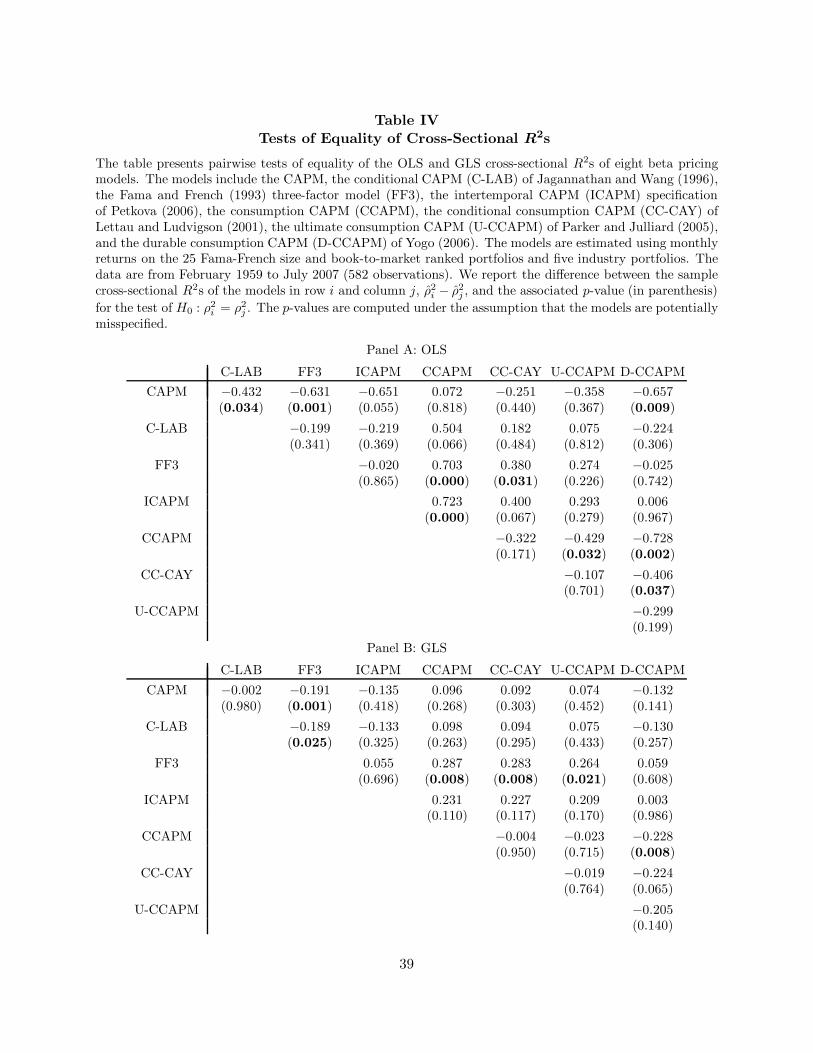
Table IV

Tests of Equality of Cross-Sectional R2s

The table presents pairwise tests of equality of the OLS and GLS cross-sectional R2s of eight beta pricingmodels. The models include the CAPM, the conditional CAPM (C-LAB) of Jagannathan and Wang (1996),the Fama and French (1993) three-factor model (FF3), the intertemporal CAPM (ICAPM) specificationof Petkova (2006), the consumption CAPM (CCAPM), the conditional consumption CAPM (CC-CAY) ofLettau and Ludvigson (2001), the ultimate consumption CAPM (U-CCAPM) of Parker and Julliard (2005),and the durable consumption CAPM (D-CCAPM) of Yogo (2006). The models are estimated using monthlyreturns on the 25 Fama-French size and book-to-market ranked portfolios and five industry portfolios. Thedata are from February 1959 to July 2007 (582 observations). We report the difference between the samplecross-sectional R2s of the models in row i and column j, ρ2

i − ρ2

j , and the associated p-value (in parenthesis)

for the test of H0 : ρ2

i = ρ2

j . The p-values are computed under the assumption that the models are potentiallymisspecified.

Panel A: OLS

C-LAB FF3 ICAPM CCAPM CC-CAY U-CCAPM D-CCAPM

CAPM −0.432 −0.631 −0.651 0.072 −0.251 −0.358 −0.657(0.034) (0.001) (0.055) (0.818) (0.440) (0.367) (0.009)

C-LAB −0.199 −0.219 0.504 0.182 0.075 −0.224(0.341) (0.369) (0.066) (0.484) (0.812) (0.306)

FF3 −0.020 0.703 0.380 0.274 −0.025(0.865) (0.000) (0.031) (0.226) (0.742)

ICAPM 0.723 0.400 0.293 0.006(0.000) (0.067) (0.279) (0.967)

CCAPM −0.322 −0.429 −0.728(0.171) (0.032) (0.002)

CC-CAY −0.107 −0.406(0.701) (0.037)

U-CCAPM −0.299(0.199)

Panel B: GLS

C-LAB FF3 ICAPM CCAPM CC-CAY U-CCAPM D-CCAPM

CAPM −0.002 −0.191 −0.135 0.096 0.092 0.074 −0.132(0.980) (0.001) (0.418) (0.268) (0.303) (0.452) (0.141)

C-LAB −0.189 −0.133 0.098 0.094 0.075 −0.130(0.025) (0.325) (0.263) (0.295) (0.433) (0.257)

FF3 0.055 0.287 0.283 0.264 0.059(0.696) (0.008) (0.008) (0.021) (0.608)

ICAPM 0.231 0.227 0.209 0.003(0.110) (0.117) (0.170) (0.986)

CCAPM −0.004 −0.023 −0.228(0.950) (0.715) (0.008)

CC-CAY −0.019 −0.224(0.764) (0.065)

U-CCAPM −0.205(0.140)

39

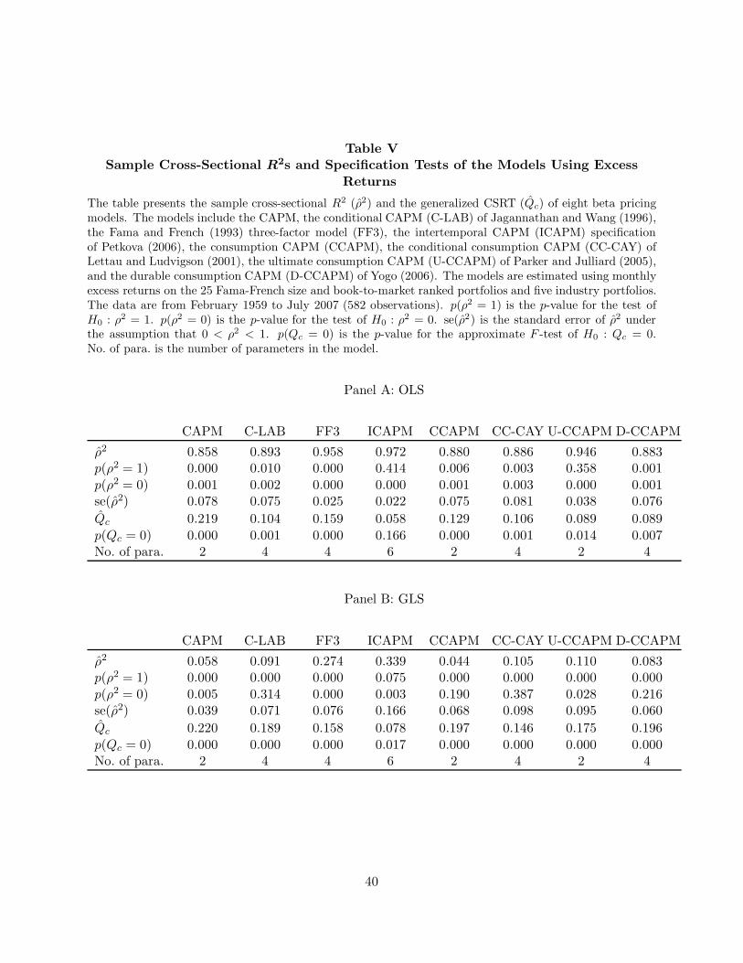
Table VSample Cross-Sectional R2s and Specification Tests of the Models Using Excess

Returns

The table presents the sample cross-sectional R2 (ρ2) and the generalized CSRT (Qc) of eight beta pricingmodels. The models include the CAPM, the conditional CAPM (C-LAB) of Jagannathan and Wang (1996),the Fama and French (1993) three-factor model (FF3), the intertemporal CAPM (ICAPM) specificationof Petkova (2006), the consumption CAPM (CCAPM), the conditional consumption CAPM (CC-CAY) ofLettau and Ludvigson (2001), the ultimate consumption CAPM (U-CCAPM) of Parker and Julliard (2005),and the durable consumption CAPM (D-CCAPM) of Yogo (2006). The models are estimated using monthlyexcess returns on the 25 Fama-French size and book-to-market ranked portfolios and five industry portfolios.The data are from February 1959 to July 2007 (582 observations). p(ρ2 = 1) is the p-value for the test ofH0 : ρ2 = 1. p(ρ2 = 0) is the p-value for the test of H0 : ρ2 = 0. se(ρ2) is the standard error of ρ2 underthe assumption that 0 < ρ2 < 1. p(Qc = 0) is the p-value for the approximate F -test of H0 : Qc = 0.No. of para. is the number of parameters in the model.

Panel A: OLS

CAPM C-LAB FF3 ICAPM CCAPM CC-CAY U-CCAPM D-CCAPM

ρ2 0.858 0.893 0.958 0.972 0.880 0.886 0.946 0.883p(ρ2 = 1) 0.000 0.010 0.000 0.414 0.006 0.003 0.358 0.001

p(ρ2 = 0) 0.001 0.002 0.000 0.000 0.001 0.003 0.000 0.001se(ρ2) 0.078 0.075 0.025 0.022 0.075 0.081 0.038 0.076

Qc 0.219 0.104 0.159 0.058 0.129 0.106 0.089 0.089

p(Qc = 0) 0.000 0.001 0.000 0.166 0.000 0.001 0.014 0.007No. of para. 2 4 4 6 2 4 2 4

Panel B: GLS

CAPM C-LAB FF3 ICAPM CCAPM CC-CAY U-CCAPM D-CCAPM

ρ2 0.058 0.091 0.274 0.339 0.044 0.105 0.110 0.083p(ρ2 = 1) 0.000 0.000 0.000 0.075 0.000 0.000 0.000 0.000

p(ρ2 = 0) 0.005 0.314 0.000 0.003 0.190 0.387 0.028 0.216se(ρ2) 0.039 0.071 0.076 0.166 0.068 0.098 0.095 0.060

Qc 0.220 0.189 0.158 0.078 0.197 0.146 0.175 0.196

p(Qc = 0) 0.000 0.000 0.000 0.017 0.000 0.000 0.000 0.000No. of para. 2 4 4 6 2 4 2 4

40

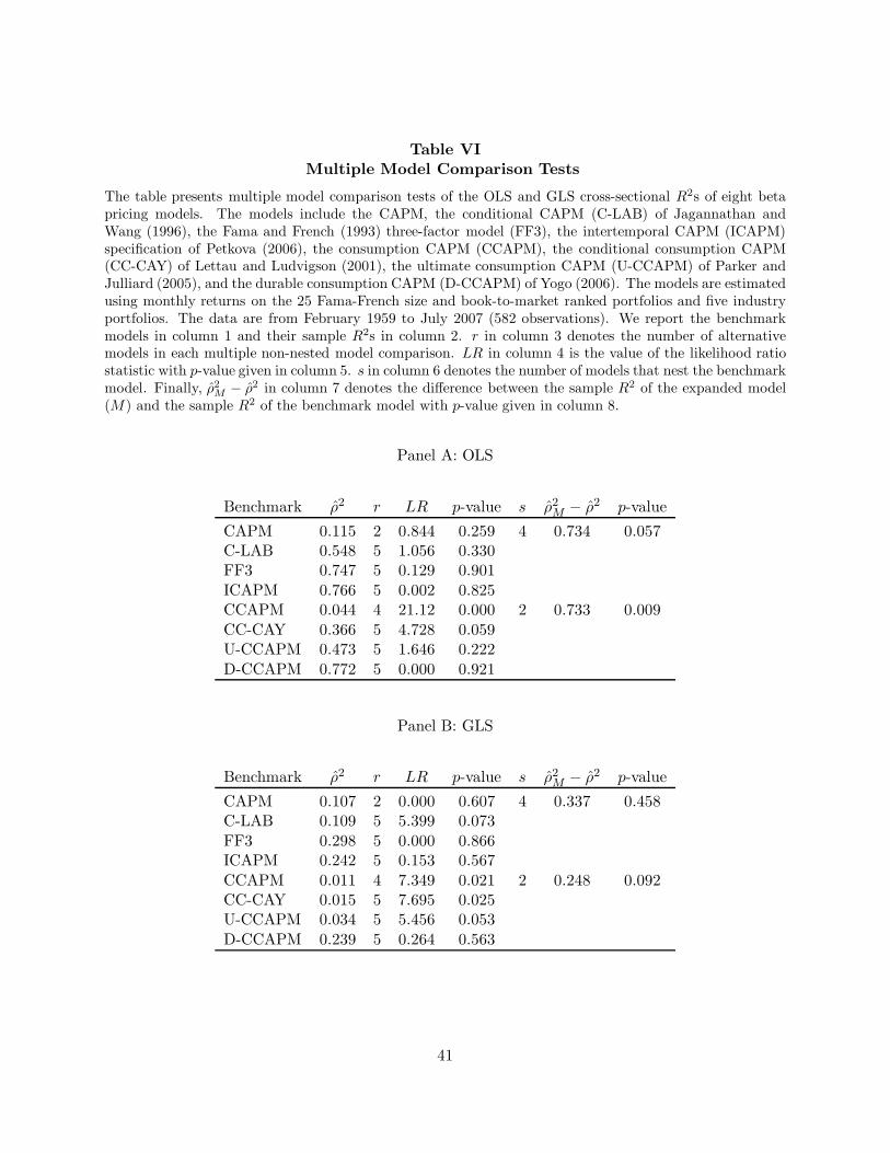
Table VIMultiple Model Comparison Tests

The table presents multiple model comparison tests of the OLS and GLS cross-sectional R2s of eight betapricing models. The models include the CAPM, the conditional CAPM (C-LAB) of Jagannathan andWang (1996), the Fama and French (1993) three-factor model (FF3), the intertemporal CAPM (ICAPM)specification of Petkova (2006), the consumption CAPM (CCAPM), the conditional consumption CAPM(CC-CAY) of Lettau and Ludvigson (2001), the ultimate consumption CAPM (U-CCAPM) of Parker andJulliard (2005), and the durable consumption CAPM (D-CCAPM) of Yogo (2006). The models are estimatedusing monthly returns on the 25 Fama-French size and book-to-market ranked portfolios and five industryportfolios. The data are from February 1959 to July 2007 (582 observations). We report the benchmarkmodels in column 1 and their sample R2s in column 2. r in column 3 denotes the number of alternativemodels in each multiple non-nested model comparison. LR in column 4 is the value of the likelihood ratiostatistic with p-value given in column 5. s in column 6 denotes the number of models that nest the benchmarkmodel. Finally, ρ2

M − ρ2 in column 7 denotes the difference between the sample R2 of the expanded model(M) and the sample R2 of the benchmark model with p-value given in column 8.

Panel A: OLS

Benchmark ρ2 r LR p-value s ρ2M − ρ2 p-value

CAPM 0.115 2 0.844 0.259 4 0.734 0.057C-LAB 0.548 5 1.056 0.330FF3 0.747 5 0.129 0.901

ICAPM 0.766 5 0.002 0.825CCAPM 0.044 4 21.12 0.000 2 0.733 0.009

CC-CAY 0.366 5 4.728 0.059U-CCAPM 0.473 5 1.646 0.222

D-CCAPM 0.772 5 0.000 0.921

Panel B: GLS

Benchmark ρ2 r LR p-value s ρ2M − ρ2 p-value

CAPM 0.107 2 0.000 0.607 4 0.337 0.458C-LAB 0.109 5 5.399 0.073

FF3 0.298 5 0.000 0.866ICAPM 0.242 5 0.153 0.567

CCAPM 0.011 4 7.349 0.021 2 0.248 0.092CC-CAY 0.015 5 7.695 0.025U-CCAPM 0.034 5 5.456 0.053

D-CCAPM 0.239 5 0.264 0.563

41