Embed Size (px)
Citation preview
Pricing Constant Maturity Credit Default Swaps
Under Jump Dynamics
Henrik Jonsson∗ and Wim Schoutens†
March 10, 2008
First version: December 15, 2007
∗Postdoctoral Research Fellow, EURANDOM P.O. Box 513, 5600MB Eindhoven, TheNetherlands. E-mail: [email protected], Phone: +31 (0)40 247 8132
†Research Professor, K.U.Leuven, Department of Mathematics, Celestijnenlaan 200 B, B-3001 Leuven, Belgium. E-mail: [email protected], Phone: +32 (0)16 32 2027
1

Abstract
In this paper we discuss the pricing of Constant Maturity Credit De-
fault Swaps (CMCDS) under single sided jump models. The CMCDS
offers default protection in exchange for a floating premium which is peri-
odically reset and indexed to the market spread on a CDS with constant
maturity tenor written on the same reference name. By setting up a firm
value model based on single sided Levy models we can generate dynamic
spreads for the reference CDS. The valuation of the CMCDS can then
easily be done by Monte Carlo simulation.
Keywords: Single sided Levy processes; Structural models; Credit risk; Defaultprobability; Constant Maturity Credit Default Swaps; Monte Carlo methodsJEL subject category: C02, C15, C63, G12
2
1 Introduction
Constant Maturity Credit Default Swaps (CMCDS) are similar to the commonCredit Default Swap (CDS), offering the investor protection in exchange of aperiodically paid spread. In contrast to the CDS spread, which is fixed throughout the maturity of the CDS, the spread of a CMCDS is floating and is indexed toa reference CDS with a fixed time to maturity at reset dates. The floating spreadis proportional to the constant maturity CDS market spread. The maturity ofthe CMCDS and of the reference CDS does not have to be the same.
The aim of this paper is to present a Monte Carlo method for estimatingthe participation rate based on single sided Levy models. We set up a firm’svalue model where the value is driven by the exponential of a Levy process withpositive drift and only negative jumps. These single sided firm’s value modelsallow us to calculate the default probabilities fast by a double Laplace inversiontechnique presented in Rogers (2000) and Madan and Schoutens (2007). Thefast calculation of the default probabilities implies a fast calculation of CDSvalues which is important for calibration. The models ability to calibrate on aCDS term structure has already been proven in Madan and Schoutens (2007).Based on the single sided firm’s value model Jonsson and Schoutens (2007)present how a dynamic spread generator can be set up that allows pricing ofexotic options on single name CDS by Monte Carlo simulations.
The paper is organized as follows. In the following section we present themechanics and valuation of Constant Maturity Credit Default Swaps. In Section3 the singel sided firm’s value model is introduced. The Monte Carlo algorithmand numerical results are given in Section 4. The paper ends with conclusions.
2 Constant Maturity Credit Default Swaps
2.1 The Mechanics of CMCDS
A single name Constant Maturity Credit Default Swap (CMCDS) has the samefeatures as a standard singel name CDS. It offers the protection buyer protectionagainst loss at the event of a default of the reference credit in exchange for aperiodically paid spread. The difference is that the spread paid is reset at pre-specified reset dates. At each reset date the CMCDS spread is set to a referenceCDS market spread times a multiplier, the so called participation rate. Thereference CDS has a constant maturity which is not necessarily the same as the
3

maturity of the CMCDS.
2.2 Valuation
We want to value a CMCDS with maturity T and M reset dates 0 = t0 < t1 <
t2 < ...tM−1 < T with a reference CDS with constant maturity tenor T . Tovalue the CMCDS is to find the participation rate, i.e. the factor we shouldmultiply the reference spread of the CDS. Just as for the CDS we equate thepresent value of the loss leg and the payment leg. However, the loss leg of theCMCDS and and the loss leg of a CDS written on the same reference name andwith the same maturity T are identical. This implies that the premium legs ofthe two contracts must be the same.
Denote by τ the default time of the reference credit.Let D(t0, t) denote the t0-value of a defaultable zero-coupon bond with ma-
turity t. We will assume that the spot rate r = {rt, t ≥ 0} is deterministic sothat the value of the defaultable zero-coupon bond is
D(t0, t) = EQ[exp
(− ∫ t
t0rsds
)1(τ > t)
]
= exp(− ∫ t
t0rsds
)PQ(τ > t),
under a risk -neutral measure Q.Assuming a constant recovery rate R the fair spread of the reference CDS
with constant maturity tenor T at time t is
S(t, t + T ) =(1−R)
(− ∫ T
0d(t, t + s)dPQ(τ > t + s|τ > t)
)
∫ T
0d(t, t + s)PQ(τ > t + s|τ > t)ds
, (1)
where d(t, t + s) = exp(− ∫ t+s
trudu
)is the riskless discount factor and the
probability of no default before time t + s, s ≥ 0, given that there was nodefault before time t, that is, the probability that the firm survives at least totime t + s given that it survived until t, is denoted by PQ(τ > t + s|τ > t).
The value of the payment at time tm+1 is based on the floating spread resetat tm, that is, for m = 0, 1, . . . , M − 1,
Zm+1(tm+1) = ∆(tm, tm+1)S(tm, tm + T )1(τ > tm+1),
with tM = T and where Zm+1(tm+1) is the time tm+1 value of the payment
4
scheduled for tm+1, ∆(tm, tm+1) is the length of the period over which the spreadis payed, expressed in the appropriate day-count convention, S(tm, tm + T )the market spread of the reference CDS at time tm, τ is the default time and1(τ > tm+1) is the survival indicator until time tm+1.
Using the defaultable zero-coupon bond with maturity tm+1 as the numerairewe can express the t0-value of the payment scheduled for tm+1 as
Zm+1(t0) = D(t0, tm+1)∆(tm, tm+1)EQm+1 [S(tm, tm + T )],
for m = 0, 1, . . . ,M − 1, where the expectation is taken with respect to therisk-neutral probability measure corresponding to the numeraire.
The t0-value of the floating premium leg is thus
FL(t0, T , T ) =M−1∑m=0
D(t0, tm+1)∆(tm, tm+1)EQm+1 [S(tm, tm + T )], (2)
with tM = T . (We have omitted any premium accrued on default for ease ofpresentation.)
As mentioned before, the values at the valuation date t0 of the fee leg ofthe CMCDS and the fee leg of a CDS written on the same reference name andwith the same maturity T must be equal. Hence we should find a participationrate p(t0, T , T ) such that the fee leg of the CMCDS equals the fee leg of a CDSwritten on the same reference name with maturity T at time t0, that is
p(t0, T , T )FL(t0, T , T ) = S(t0, T )PV01(t0, T ), (3)
where PV01(t0, T ) is the time t0 risky annuity of a CDS with the same maturityand written on the same reference credit as the CMCDS, that is, the t0-valueof the premium leg assuming a premium of 1 basis point
PV01(t0, T ) =∫ T
t0
exp(−
∫ s
t0
rudu
)PQ(τ > s)ds.
Thus, from (3) we have that the participation rate is
p(t0, T , T ) =S(t0, T )
∫ T
t0exp
(− ∫ s
t0rudu
)PQ(τ > s)ds
∑M−1m=0 D(t0, tm+1)∆(tm, tm+1)EQm+1 [S(tm, tm + T )]
. (4)
5

2.3 Caps and Floors
A natural extension of the floating premium CMCDS is to incorporate a cap.Following Pedersen and Sen (2004) we will assume that the cap acts directly onthe reset spread. The cap is a portfolio of caplets. A caplet is an European calloption and is used to limit the spread paid.
Denote by KC the spread cap. The t0-value of the caplet at reset date tm+1,ignoring premium accrual on default, is
Cm+1(t0) = D(t0, tm+1)∆(tm, tm+1)EQm+1 [(S(tm, tm + T )−KC)+].
The t0-value of the cap is the sum of the t0-values of the caplets
C(t0) =M−1∑m=0
Cm+1(t0).
Similarly, with KF denoting the spread floor, the t0-value of the floorlet atthe reset date tm+1 is
Fm+1(t0) = D(t0, tm+1)∆(tm, tm+1)EQm+1 [(KF − S(tm, tm + T ))+],
and t0-value of the floor, that is, the portfolio of floorlets,
F (t0) =M−1∑m=0
Fm+1(t0).
2.4 Mark-to-Market
The mark-to-market of a CMCDS is done by comparing the present value of thecontract floating fee leg with the market value of the protection leg. The valueof the protection leg at a time t, t0 ≤ t ≤ T , is S(t, T )PV01(t, T ). The valueof the floating fee leg is pt0FL(t, T , T ). The mark-to-market for the protectionseller is thus
MTMCMCDS(t) =
(p(t0, T , T )p(t, T , T )
− 1
)S(t, T )PV01(t, T ),
since the floating fee leg at time t is equal to the protection leg at time t dividedby the participation rate at t, i.e., FL(t, T , T ) = S(t, T )PV01(t, T )/p(t, T , T ).
The mark-to-market of a standard CDS with maturity T is for the protection
6
sellerMTMCDS(t) =
(S(t0, T )− S(t, T )
)PV01(t, T ).
2.5 Valuation Using Forward Spreads and Convexity Ad-
justment
A first approximation to the value of the floating fee leg is to approximate theexpected market spread at the reset dates with the forward spread at time t0.The forward spread is the fair spread for a forward starting CDS. Denote byS(t0, t, t + T ) the forward spread at time t0 of a CDS starting at time t withmaturity t + T . Its value is given by
S(t0, t, t + T ) =S(t0, t + T )PV01(t0, t + T )− S(t0, t)PV01(t0, t)
PV01(t0, t + T )− PV01(t0, t).
Substituting the expected spreads in (2) with the forward spreads the t0-value of the fee leg is approximated by
FL(t0, T , T ) ≈M−1∑m=0
D(t0, tm+1)∆(tm, tm+1)S(t0, tm, tm + T ), (5)
where S(t0, t0, t0 + T ) = S(t0, t0 + T ).We need however to adjust this approximation since the realized spread at
the reset dates are not equal to the forward spreads calculated at the valuationdate t0. The adjustment that has to be added to the fee leg is called the convexityadjustment and is given by
A(t0; T , T ) =M−1∑m=1
D(t0, tm+1)∆(tm, tm+1)A(tm, tm + T ), (6)
where for m = 1, . . . , M − 1
A(tm, tm + T ) = EQm+1 [S(tm, tm + T )]− S(t0, tm, tm + T ).
3 Single Sided Firm’s Value Model
Levy models have proven their usefulness in financial modelling, such as in equityand fixed income settings, over the last decade, see e.g. Schoutens (2003), andhas recently gained growing interest in credit risk modelling, see e.g. Cariboni
7
(2007) and Cariboni and Schoutens (2007).We will in this section set up the single sided firm’s value model presented in
Madan and Schoutens (2007). We thus model the value of the reference entity ofa CDS by exponential Levy driven models with positive drift and only negativejumps. Following the same methodology as Black and Cox (1976) default istriggered the first time the firm’s value is crossing a low barrier. The modelswere used to construct spread dynamics to price exotic credit default swaptionsin Jonsson and Schoutens (2007).
3.1 Single Sided Levy Processes
We first introduce some notation. Let Y = {Yt, t ≥ 0} be a pure jump Levyprocess that has only negative jumps, that is, Y is spectrally negative, and letX = {Xt, t ≥ 0} be given by
Xt = µt + Yt, t ≥ 0,
where µ is positive real number.The Laplace transform of Xt
E[exp(zXt)] = exp(tψX(z)),
where ψX(z) is the Levy exponent, which by the Levy-Khintchin representationhas the form
ψX(z) = µz +∫ 0
−∞(ezx − 1 + z(|x| ∧ 1))ν(dx).
The Levy measure ν(dx) satisfies the integrability condition
∫ 0
−∞(|x| ∧ 1)ν(dx) < ∞.
For the processes we consider in this paper the Levy measure has a densityand we can write ν(dx) = m(x)dx, where m(x) is the density function. Forthe general theory of Levy processes see, for example, Bertoin (1996) and Sato(2000).
8
3.2 Firm’s Value Model
Let X = {Xt, t ≥ 0} be a pure jump Levyprocess. The risk neutral value of thefirm at time t is then
Vt = V0 exp(Xt), t ≥ 0,
and we work under an admissible pricing measure Q.For a given recovery rate R default occurs the first time the firm’s value is
below the value RV0. That is, the time of default is defined as
τ := inf{t ≥ 0 : Vt ≤ RV0}.
Let us denote by P(t) := PQ(τ > t) the risk-neutral survival probabilitybetween 0 and t:
P(t) = PQ (Xs > log R, for all 0 ≤ s ≤ t)
= PQ
(min
0≤s≤tXS > log R
)
= EQ[1
(min
0≤s≤tXs > log R
)]
= EQ[1
(min
0≤s≤tVs > RV0
)]
where we used the indicator function 1(A), which is equal to 1 if the event A istrue and zero otherwise; the subindex Q refers to the fact that we are workingin a risk-neutral setting.
As can be seen in (1) and (4) the price of the CDS and the participationrate of the CMCDS, respectively, depends on the survival probability, or non-default probability, of the firm. In our case, where we work under single sidedLevymodels with positive drift and only negative jumps, the default probabilitiescan be calculated by a double Laplace inversion based on the Wiener-Hopffactorization as presented in Madan and Schoutens (2007).
3.3 Example - The Shifted Gamma-Model
Three well known examples of single sided jump models with positive drift werepresented in Madan and Schoutens (2007), namely: the Shifted Gamma, theShifted Inverse Gaussian and the Shifted CMY model. We present here indetail only the Shifted Gamma model.
9
The density function of the Gamma distribution Gamma(a, b) with param-eters a > 0 and b > 0 is given by
fGamma(x; a, b) =ba
Γ(a)xa−1 exp(−xb), x > 0.
The characteristic function is given by
φGamma(u; a, b) = (1− iu/b)−a, u ∈ R.
Clearly, this characteristic function is infinitely divisible. The Gamma-process G = {Gt, t ≥ 0} with parameters a, b > 0 is defined as the stochasticprocess which starts at zero and has stationary, independent Gamma-distributedincrements. More precisely, the time enters in the first parameter: Gt follows aGamma(at, b) distribution.
The Levy density of the Gamma process is given by
m(x) = a exp(−bx)x−1, x > 0.
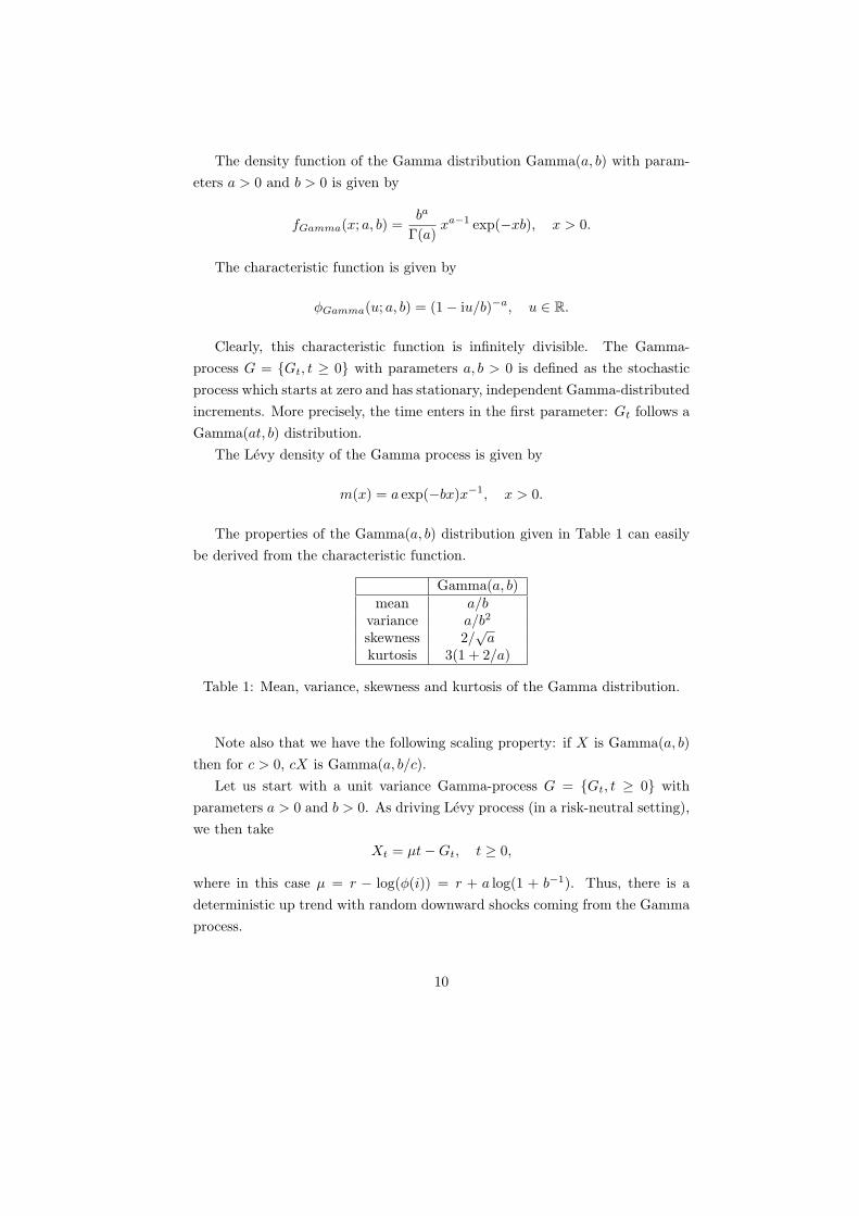
The properties of the Gamma(a, b) distribution given in Table 1 can easilybe derived from the characteristic function.
Gamma(a, b)mean a/b
variance a/b2
skewness 2/√
akurtosis 3(1 + 2/a)
Table 1: Mean, variance, skewness and kurtosis of the Gamma distribution.
Note also that we have the following scaling property: if X is Gamma(a, b)then for c > 0, cX is Gamma(a, b/c).
Let us start with a unit variance Gamma-process G = {Gt, t ≥ 0} withparameters a > 0 and b > 0. As driving Levy process (in a risk-neutral setting),we then take
Xt = µt−Gt, t ≥ 0,
where in this case µ = r − log(φ(i)) = r + a log(1 + b−1). Thus, there is adeterministic up trend with random downward shocks coming from the Gammaprocess.
10
The characteristic exponent is in this case available in closed form
ψ(z) = µz − a log(1 + zb−1).
3.3.1 Calibration
We have calibrated the Shifted Gamma model to the term structure of ABN-AMRO CDSs minimizing the average absolute percentage error
APE =1
mean CDS spread
∑
CDS
|market CDS spread−model CDS spread|number of CDSs
.
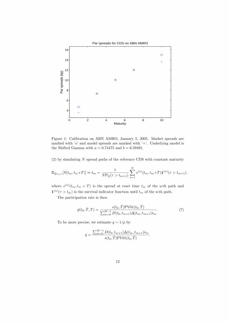
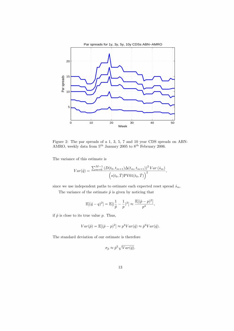
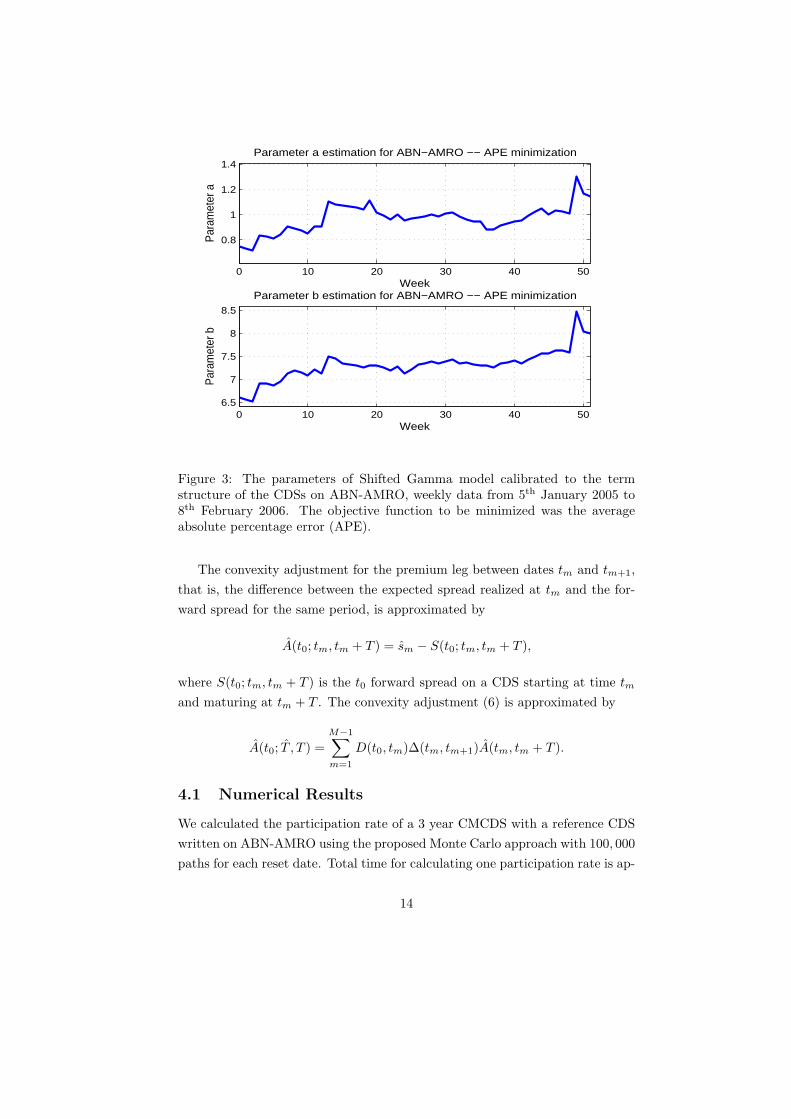
Calibrating the Shifted Gamma model to the term structure of ABN-AMROon the 5th of January 2005 gives the parameters a = 0.74475 and b = 6.59491.The fit of the Shifted Gamma model on the market CDSs is shown in Figure1. The evolution of 1, 3, 5, 7 and 10 years par spreads of the ABN-AMROCDSs from 5th January 2005 to 8th February 2006 is shown in Figure 2. Theevolution over time of the parameters of the Shifted Gamma model calibratedon the term structure is shown in Figure 3.
An extensive calibration study was performed by Madan and Schoutens(2007) and the fitting error was typically around 1-2 basis points per quote.
4 A Monte Carlo Valuation Approach
As seen from (2) we need a model for the spread dynamics of the reference CDSwith constant maturity. We will use the spread dynamics developed in Jonssonand Schoutens (2007).
The method is based on four steps. The first step is to calibrate the modelon a given term structure of market spreads. The calibration gives us themodel parameters that best matches the current market situation. Next weprecalculate for a fine grid of firm values {v1, . . . , vK} the corresponding spreadvalues {S(vi, R, r, T, θ), i = 1, . . . , K} by using the fast way of calculating thedefault probabilities presented by Madan and Schoutens (2007). The third stepis to generate firm’s value paths on a time gride. Finally, for every path and eachvalue on the time grid the corresponding spread is obtained by interpolatingthe simulated firm value in {v1, . . . , vK} and its corresponding spread values{S(vi, R, r, T, θ), i = 1, . . . , K}.
For each reset date tm, m = 0, 1, . . . , M − 1, estimate the expected value in
11
0 2 4 6 8 10
4
6
8
10
12
14
16
Maturity
Par
spr
eads
(bp)
Par spreads for CDS on ABN AMRO
Figure 1: Calibration on ABN AMRO, January 5, 2005. Market spreads aremarked with ’o’ and model spreads are marked with ’+’. Underlying model isthe Shifted Gamma with a = 0.74475 and b = 6.59491.
(2) by simulating N spread paths of the reference CDS with constant maturity
EQm+1 [S(tm, tm+T )] ≈ sm =1
NPQ(τ > tm+1)
N∑n=1
s(n)(tm, tm+T )1(n)(τ > tm+1),
where s(n)(tm, tm + T ) is the spread at reset time tm of the n:th path and1(n)(τ > tm) is the survival indicator function until tm of the n:th path.
The participation rate is then
p(t0, T , T ) =s(t0, T )PV01(t0, T )∑M−1
m=0 D(t0, tm+1)∆(tm, tm+1)sm
. (7)
To be more precise, we estimate q = 1/p by
q =∑M−1
m=0 D(t0, tm+1)∆(tm, tm+1)sm
s(t0, T )PV01(t0, T ).
12
0 10 20 30 40 50
5
10
15
20
Week
Par
spr
eads
Par spreads for 1y, 3y, 5y, 10y CDSs ABN−AMRO
Figure 2: The par spreads of a 1, 3, 5, 7 and 10 year CDS spreads on ABN-AMRO, weekly data from 5th January 2005 to 8th February 2006.
The variance of this estimate is
V ar(q) =∑M−1
m=0 (D(t0, tm+1)∆(tm, tm+1))2V ar (sm)(
s(t0, T )PV01(t0, T ))2 ,
since we use independent paths to estimate each expected reset spread sm.The variance of the estimate p is given by noticing that
E[(q − q)2] = E[(1p− 1
p)2] ≈ E[(p− p)2]
p4,
if p is close to its true value p. Thus,
V ar(p) = E[(p− p)2] ≈ p4V ar(q) ≈ p4V ar(q).
The standard deviation of our estimate is therefore
σp ≈ p2√
V ar(q).
13
0 10 20 30 40 50
0.8
1
1.2
1.4
Week
Par
amet
er a
Parameter a estimation for ABN−AMRO −− APE minimization
0 10 20 30 40 506.5
7
7.5
8
8.5
Week
Par
amet
er b
Parameter b estimation for ABN−AMRO −− APE minimization
Figure 3: The parameters of Shifted Gamma model calibrated to the termstructure of the CDSs on ABN-AMRO, weekly data from 5th January 2005 to8th February 2006. The objective function to be minimized was the averageabsolute percentage error (APE).
The convexity adjustment for the premium leg between dates tm and tm+1,that is, the difference between the expected spread realized at tm and the for-ward spread for the same period, is approximated by
A(t0; tm, tm + T ) = sm − S(t0; tm, tm + T ),
where S(t0; tm, tm + T ) is the t0 forward spread on a CDS starting at time tm
and maturing at tm + T . The convexity adjustment (6) is approximated by
A(t0; T , T ) =M−1∑m=1
D(t0, tm)∆(tm, tm+1)A(tm, tm + T ).
4.1 Numerical Results
We calculated the participation rate of a 3 year CMCDS with a reference CDSwritten on ABN-AMRO using the proposed Monte Carlo approach with 100, 000paths for each reset date. Total time for calculating one participation rate is ap-
14
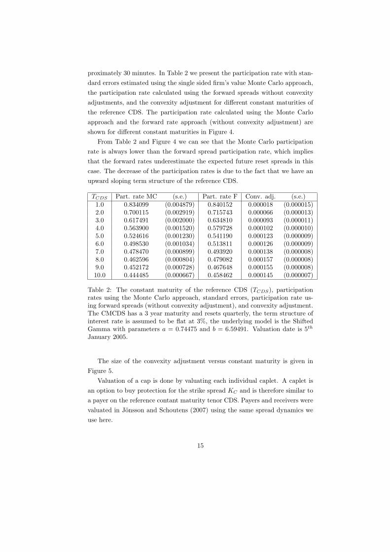
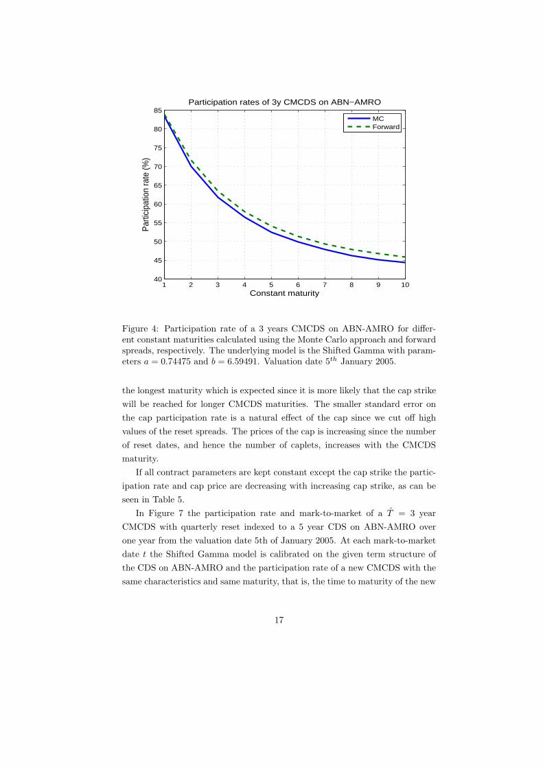
proximately 30 minutes. In Table 2 we present the participation rate with stan-dard errors estimated using the single sided firm’s value Monte Carlo approach,the participation rate calculated using the forward spreads without convexityadjustments, and the convexity adjustment for different constant maturities ofthe reference CDS. The participation rate calculated using the Monte Carloapproach and the forward rate approach (without convexity adjustment) areshown for different constant maturities in Figure 4.
From Table 2 and Figure 4 we can see that the Monte Carlo participationrate is always lower than the forward spread participation rate, which impliesthat the forward rates underestimate the expected future reset spreads in thiscase. The decrease of the participation rates is due to the fact that we have anupward sloping term structure of the reference CDS.
TCDS Part. rate MC (s.e.) Part. rate F Conv. adj. (s.e.)1.0 0.834099 (0.004879) 0.840152 0.000018 (0.000015)2.0 0.700115 (0.002919) 0.715743 0.000066 (0.000013)3.0 0.617491 (0.002000) 0.634810 0.000093 (0.000011)4.0 0.563900 (0.001520) 0.579728 0.000102 (0.000010)5.0 0.524616 (0.001230) 0.541190 0.000123 (0.000009)6.0 0.498530 (0.001034) 0.513811 0.000126 (0.000009)7.0 0.478470 (0.000899) 0.493920 0.000138 (0.000008)8.0 0.462596 (0.000804) 0.479082 0.000157 (0.000008)9.0 0.452172 (0.000728) 0.467648 0.000155 (0.000008)10.0 0.444485 (0.000667) 0.458462 0.000145 (0.000007)
Table 2: The constant maturity of the reference CDS (TCDS), participationrates using the Monte Carlo approach, standard errors, participation rate us-ing forward spreads (without convexity adjustment), and convexity adjustment.The CMCDS has a 3 year maturity and resets quarterly, the term structure ofinterest rate is assumed to be flat at 3%, the underlying model is the ShiftedGamma with parameters a = 0.74475 and b = 6.59491. Valuation date is 5th
January 2005.
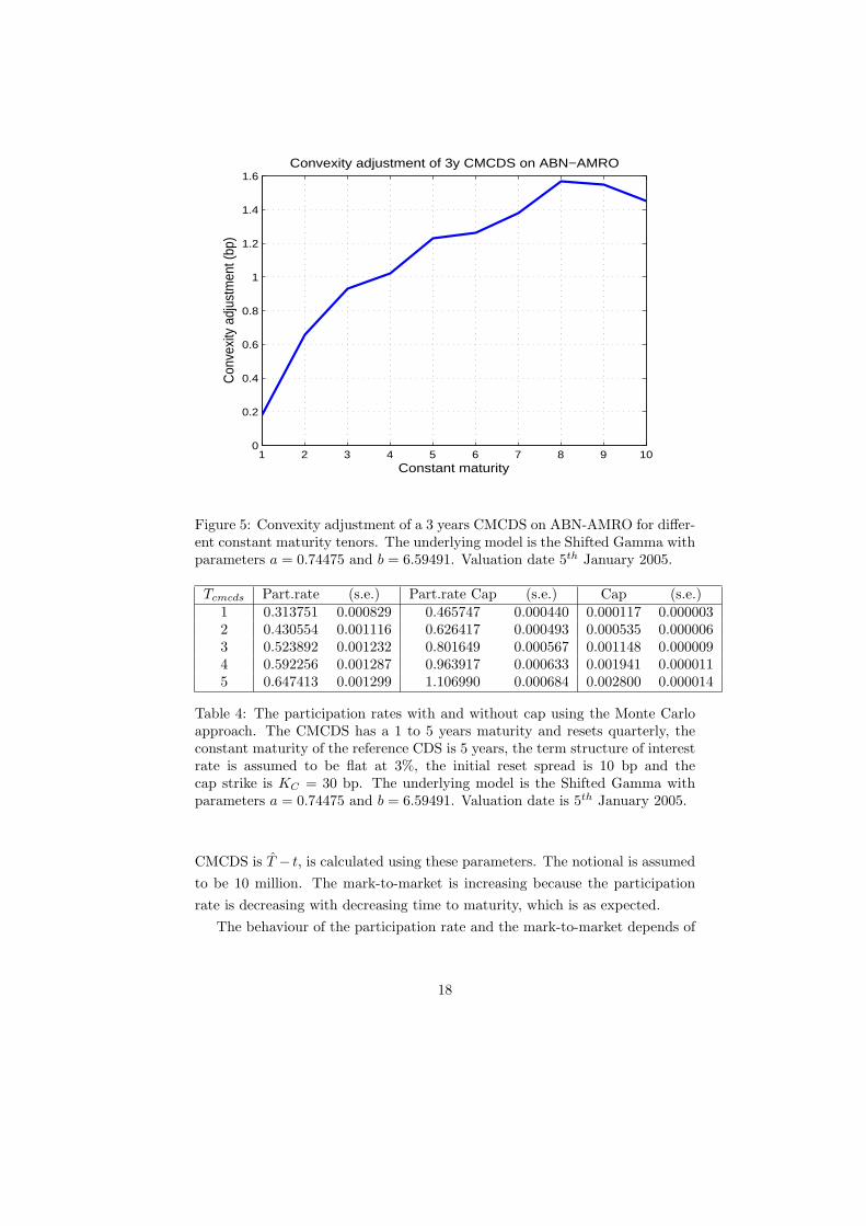
The size of the convexity adjustment versus constant maturity is given inFigure 5.
Valuation of a cap is done by valuating each individual caplet. A caplet isan option to buy protection for the strike spread KC and is therefore similar toa payer on the reference contant maturity tenor CDS. Payers and receivers werevaluated in Jonsson and Schoutens (2007) using the same spread dynamics weuse here.
15
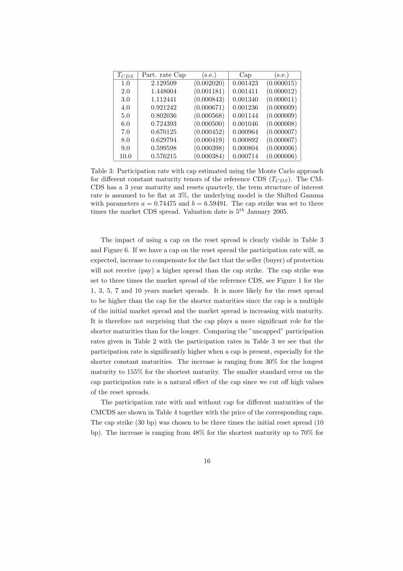
TCDS Part. rate Cap (s.e.) Cap (s.e.)1.0 2.129509 (0.002020) 0.001423 (0.000015)2.0 1.448004 (0.001181) 0.001411 (0.000012)3.0 1.112441 (0.000843) 0.001340 (0.000011)4.0 0.921242 (0.000671) 0.001236 (0.000009)5.0 0.802036 (0.000568) 0.001144 (0.000009)6.0 0.724393 (0.000500) 0.001046 (0.000008)7.0 0.670125 (0.000452) 0.000964 (0.000007)8.0 0.629794 (0.000419) 0.000892 (0.000007)9.0 0.599598 (0.000398) 0.000804 (0.000006)10.0 0.576215 (0.000384) 0.000714 (0.000006)
Table 3: Participation rate with cap estimated using the Monte Carlo approachfor different constant maturity tenors of the reference CDS (TCDS). The CM-CDS has a 3 year maturity and resets quarterly, the term structure of interestrate is assumed to be flat at 3%, the underlying model is the Shifted Gammawith parameters a = 0.74475 and b = 6.59491. The cap strike was set to threetimes the market CDS spread. Valuation date is 5th January 2005.
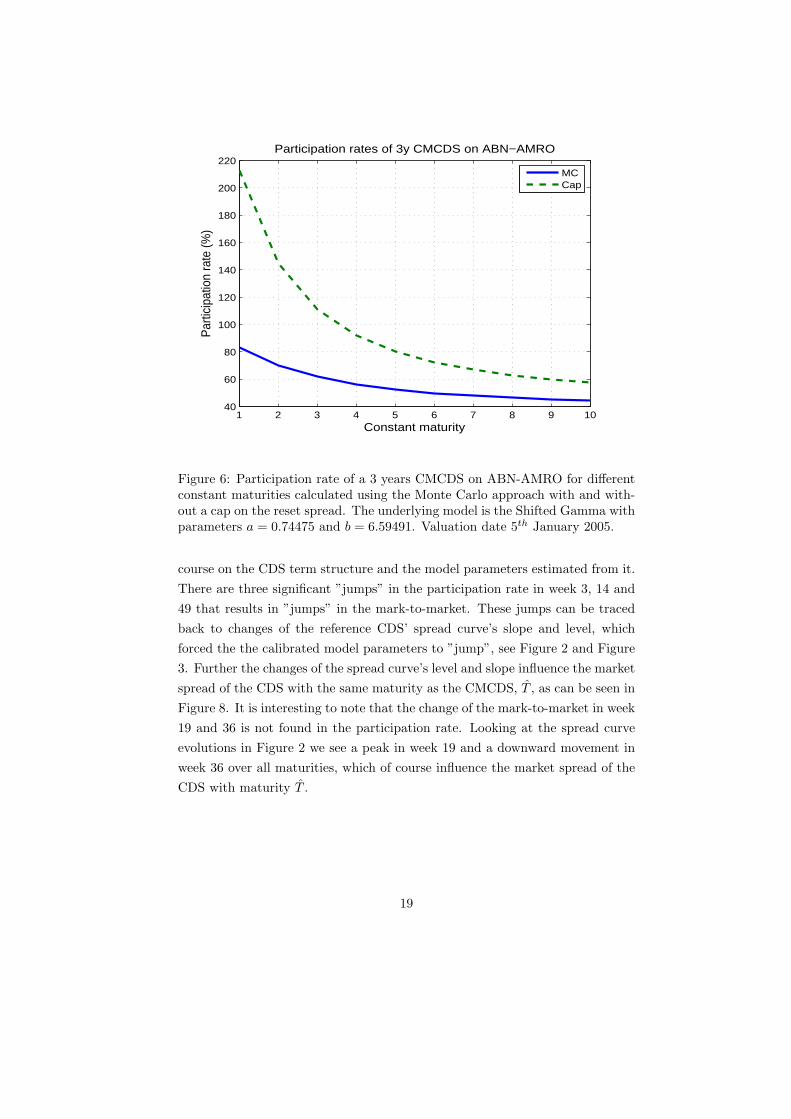
The impact of using a cap on the reset spread is clearly visible in Table 3and Figure 6. If we have a cap on the reset spread the participation rate will, asexpected, increase to compensate for the fact that the seller (buyer) of protectionwill not receive (pay) a higher spread than the cap strike. The cap strike wasset to three times the market spread of the reference CDS, see Figure 1 for the1, 3, 5, 7 and 10 years market spreads. It is more likely for the reset spreadto be higher than the cap for the shorter maturities since the cap is a multipleof the initial market spread and the market spread is increasing with maturity.It is therefore not surprising that the cap plays a more significant role for theshorter maturities than for the longer. Comparing the ”uncapped” participationrates given in Table 2 with the participation rates in Table 3 we see that theparticipation rate is significantly higher when a cap is present, especially for theshorter constant maturities. The increase is ranging from 30% for the longestmaturity to 155% for the shortest maturity. The smaller standard error on thecap participation rate is a natural effect of the cap since we cut off high valuesof the reset spreads.
The participation rate with and without cap for different maturities of theCMCDS are shown in Table 4 together with the price of the corresponding caps.The cap strike (30 bp) was chosen to be three times the initial reset spread (10bp). The increase is ranging from 48% for the shortest maturity up to 70% for
16
1 2 3 4 5 6 7 8 9 1040
45
50
55
60
65
70
75
80
85Participation rates of 3y CMCDS on ABN−AMRO
Par
ticip
atio
n ra
te (%
)
Constant maturity
MCForward
Figure 4: Participation rate of a 3 years CMCDS on ABN-AMRO for differ-ent constant maturities calculated using the Monte Carlo approach and forwardspreads, respectively. The underlying model is the Shifted Gamma with param-eters a = 0.74475 and b = 6.59491. Valuation date 5th January 2005.
the longest maturity which is expected since it is more likely that the cap strikewill be reached for longer CMCDS maturities. The smaller standard error onthe cap participation rate is a natural effect of the cap since we cut off highvalues of the reset spreads. The prices of the cap is increasing since the numberof reset dates, and hence the number of caplets, increases with the CMCDSmaturity.
If all contract parameters are kept constant except the cap strike the partic-ipation rate and cap price are decreasing with increasing cap strike, as can beseen in Table 5.
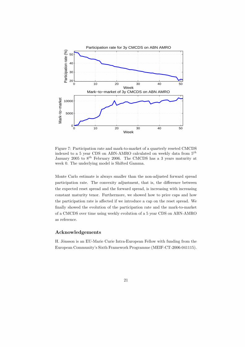
In Figure 7 the participation rate and mark-to-market of a T = 3 yearCMCDS with quarterly reset indexed to a 5 year CDS on ABN-AMRO overone year from the valuation date 5th of January 2005. At each mark-to-marketdate t the Shifted Gamma model is calibrated on the given term structure ofthe CDS on ABN-AMRO and the participation rate of a new CMCDS with thesame characteristics and same maturity, that is, the time to maturity of the new
17
1 2 3 4 5 6 7 8 9 100
0.2
0.4
0.6
0.8
1
1.2
1.4
1.6Convexity adjustment of 3y CMCDS on ABN−AMRO
Con
vexi
ty a
djus
tmen
t (bp
)
Constant maturity
Figure 5: Convexity adjustment of a 3 years CMCDS on ABN-AMRO for differ-ent constant maturity tenors. The underlying model is the Shifted Gamma withparameters a = 0.74475 and b = 6.59491. Valuation date 5th January 2005.
Tcmcds Part.rate (s.e.) Part.rate Cap (s.e.) Cap (s.e.)1 0.313751 0.000829 0.465747 0.000440 0.000117 0.0000032 0.430554 0.001116 0.626417 0.000493 0.000535 0.0000063 0.523892 0.001232 0.801649 0.000567 0.001148 0.0000094 0.592256 0.001287 0.963917 0.000633 0.001941 0.0000115 0.647413 0.001299 1.106990 0.000684 0.002800 0.000014
Table 4: The participation rates with and without cap using the Monte Carloapproach. The CMCDS has a 1 to 5 years maturity and resets quarterly, theconstant maturity of the reference CDS is 5 years, the term structure of interestrate is assumed to be flat at 3%, the initial reset spread is 10 bp and thecap strike is KC = 30 bp. The underlying model is the Shifted Gamma withparameters a = 0.74475 and b = 6.59491. Valuation date is 5th January 2005.
CMCDS is T − t, is calculated using these parameters. The notional is assumedto be 10 million. The mark-to-market is increasing because the participationrate is decreasing with decreasing time to maturity, which is as expected.
The behaviour of the participation rate and the mark-to-market depends of
18
1 2 3 4 5 6 7 8 9 1040
60
80
100
120
140
160
180
200
220Participation rates of 3y CMCDS on ABN−AMRO
Par
ticip
atio
n ra
te (%
)
Constant maturity
MCCap
Figure 6: Participation rate of a 3 years CMCDS on ABN-AMRO for differentconstant maturities calculated using the Monte Carlo approach with and with-out a cap on the reset spread. The underlying model is the Shifted Gamma withparameters a = 0.74475 and b = 6.59491. Valuation date 5th January 2005.
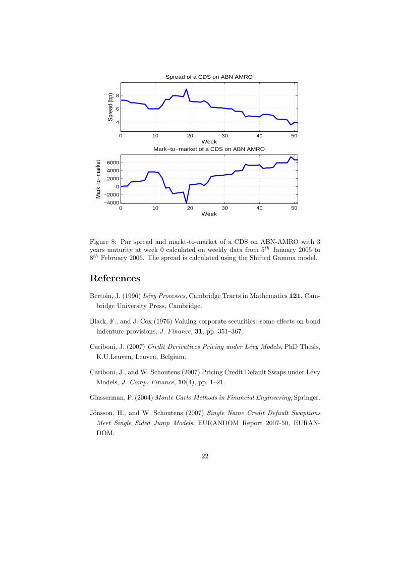
course on the CDS term structure and the model parameters estimated from it.There are three significant ”jumps” in the participation rate in week 3, 14 and49 that results in ”jumps” in the mark-to-market. These jumps can be tracedback to changes of the reference CDS’ spread curve’s slope and level, whichforced the the calibrated model parameters to ”jump”, see Figure 2 and Figure3. Further the changes of the spread curve’s level and slope influence the marketspread of the CDS with the same maturity as the CMCDS, T , as can be seen inFigure 8. It is interesting to note that the change of the mark-to-market in week19 and 36 is not found in the participation rate. Looking at the spread curveevolutions in Figure 2 we see a peak in week 19 and a downward movement inweek 36 over all maturities, which of course influence the market spread of theCDS with maturity T .
19
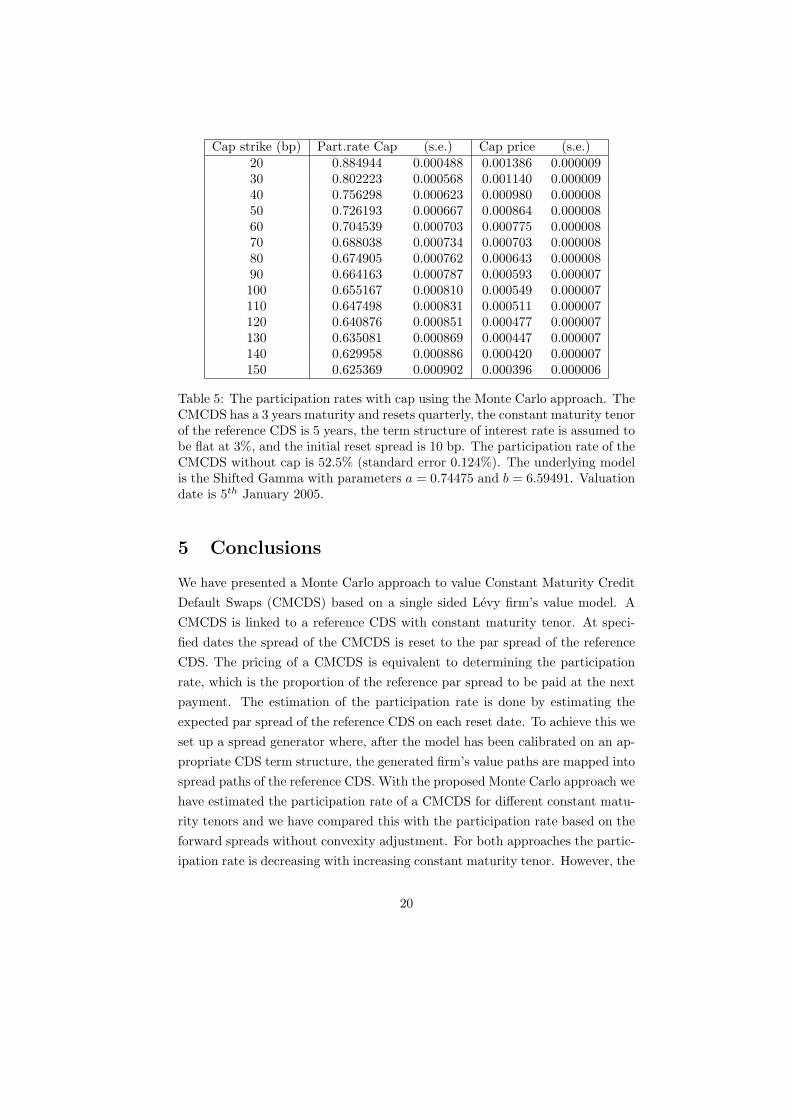
Cap strike (bp) Part.rate Cap (s.e.) Cap price (s.e.)20 0.884944 0.000488 0.001386 0.00000930 0.802223 0.000568 0.001140 0.00000940 0.756298 0.000623 0.000980 0.00000850 0.726193 0.000667 0.000864 0.00000860 0.704539 0.000703 0.000775 0.00000870 0.688038 0.000734 0.000703 0.00000880 0.674905 0.000762 0.000643 0.00000890 0.664163 0.000787 0.000593 0.000007100 0.655167 0.000810 0.000549 0.000007110 0.647498 0.000831 0.000511 0.000007120 0.640876 0.000851 0.000477 0.000007130 0.635081 0.000869 0.000447 0.000007140 0.629958 0.000886 0.000420 0.000007150 0.625369 0.000902 0.000396 0.000006
Table 5: The participation rates with cap using the Monte Carlo approach. TheCMCDS has a 3 years maturity and resets quarterly, the constant maturity tenorof the reference CDS is 5 years, the term structure of interest rate is assumed tobe flat at 3%, and the initial reset spread is 10 bp. The participation rate of theCMCDS without cap is 52.5% (standard error 0.124%). The underlying modelis the Shifted Gamma with parameters a = 0.74475 and b = 6.59491. Valuationdate is 5th January 2005.
5 Conclusions
We have presented a Monte Carlo approach to value Constant Maturity CreditDefault Swaps (CMCDS) based on a single sided Levy firm’s value model. ACMCDS is linked to a reference CDS with constant maturity tenor. At speci-fied dates the spread of the CMCDS is reset to the par spread of the referenceCDS. The pricing of a CMCDS is equivalent to determining the participationrate, which is the proportion of the reference par spread to be paid at the nextpayment. The estimation of the participation rate is done by estimating theexpected par spread of the reference CDS on each reset date. To achieve this weset up a spread generator where, after the model has been calibrated on an ap-propriate CDS term structure, the generated firm’s value paths are mapped intospread paths of the reference CDS. With the proposed Monte Carlo approach wehave estimated the participation rate of a CMCDS for different constant matu-rity tenors and we have compared this with the participation rate based on theforward spreads without convexity adjustment. For both approaches the partic-ipation rate is decreasing with increasing constant maturity tenor. However, the
20
0 10 20 30 40 5020
30
40
50
Week
Par
ticip
atio
n ra
te (%
) Participation rate for 3y CMCDS on ABN AMRO
0 10 20 30 40 500
5000
10000
Week
Mar
k−to
−mar
ket
Mark−to−market of 3y CMCDS on ABN AMRO
Figure 7: Participation rate and mark-to-market of a quarterly reseted CMCDSindexed to a 5 year CDS on ABN-AMRO calculated on weekly data from 5th
January 2005 to 8th February 2006. The CMCDS has a 3 years maturity atweek 0. The underlying model is Shifted Gamma.
Monte Carlo estimate is always smaller than the non-adjusted forward spreadparticipation rate. The convexity adjustment, that is, the difference betweenthe expected reset spread and the forward spread, is increasing with increasingconstant maturity tenor. Furthermore, we showed how to price caps and howthe participation rate is affected if we introduce a cap on the reset spread. Wefinally showed the evolution of the participation rate and the mark-to-marketof a CMCDS over time using weekly evolution of a 5 year CDS on ABN-AMROas reference.
Acknowledgements
H. Jonsson is an EU-Marie Curie Intra-European Fellow with funding from theEuropean Community’s Sixth Framework Programme (MEIF-CT-2006-041115).
21
0 10 20 30 40 50
4
6
8
Week
Spr
ead
(bp)
Spread of a CDS on ABN AMRO
0 10 20 30 40 50−4000
−2000
0
2000
4000
6000
Week
Mar
k−to
−mar
ket
Mark−to−market of a CDS on ABN AMRO
Figure 8: Par spread and markt-to-market of a CDS on ABN-AMRO with 3years maturity at week 0 calculated on weekly data from 5th January 2005 to8th February 2006. The spread is calculated using the Shifted Gamma model.
References
Bertoin, J. (1996) Levy Processes, Cambridge Tracts in Mathematics 121, Cam-bridge University Press, Cambridge.
Black, F., and J. Cox (1976) Valuing corporate securities: some effects on bondindenture provisions, J. Finance, 31, pp. 351–367.
Cariboni, J. (2007) Credit Derivatives Pricing under Levy Models, PhD Thesis,K.U.Leuven, Leuven, Belgium.
Cariboni, J., and W. Schoutens (2007) Pricing Credit Default Swaps under LevyModels, J. Comp. Finance, 10(4), pp. 1–21.
Glasserman, P. (2004) Monte Carlo Methods in Financial Engineering, Springer.
Jonsson, H., and W. Schoutens (2007) Single Name Credit Default SwaptionsMeet Single Sided Jump Models. EURANDOM Report 2007-50, EURAN-DOM.
22

Madan, D. B., and W. Schoutens (2007) Break on Through to the Single Side.Section of Statistics Technical Report 07-05, K.U.Leuven, Leuven.
Pedersen, C.M., and S. Sen (2004) Valuation of Constant Maturity DefaultSwaps. Technical Report, Lehman Brothers. Quantitative Credit ResearchQuarterly.
Rogers, L.C.G. (2000) Evaluating first-passage probabilities for spectrally one-sided Levy processes. J. Appl. Probability 37, pp. 1173-1180.
Sato, K. (2000) Levy Processes and Infinitely Divisible Distributions. Cam-bridge Studies in Advanced Mathematics 68, Cambridge University Press,Cambridge.
Schoutens, W. (2003) Levy Processes in Finance: Pricing Financial Derivatives,Wiley.
23