WP/04/27

Equity Prices, Credit Default Swaps, and Bond Spreads in Emerging Markets

Jorge A. Chan-Lau and Yoon Sook Kim

© 2004 International Monetary Fund WP/04/27

IMF Working Paper

International Capital Markets

Equity Prices, Credit Default Swaps, and Bond Spreads in Emerging Markets1

Prepared by Jorge A. Chan-Lau and Yoon Sook Kim

Authorized for distribution by Todd Groome and Donald J. Mathieson

February 2004

Abstract

This Working Paper should not be reported as representing the views of the IMF. The views expressed in this Working Paper are those of the author(s) and do not necessarily represent those of the IMF or IMF policy. Working Papers describe research in progress by the author(s) and are published to elicit comments and to further debate.

This paper examines equilibrium price relationships and price discovery between credit defaul swap (CDS), bond, and equity markets for emerging market sovereign issuers. Findings suggest that CDS and bond spreads converge despite various pressures that arise in the market. In most countries, however, we do not find any equilibrium price relationship between the bond and CDS markets and the equity markets. As for price discovery, our results are mixed. This stands in contrast to the empirical findings on corporate issuers in theUnited States and Europe. JEL Classification Numbers: G10, G14, G15 Keywords: Credit derivatives, bond spreads, equity prices, price discovery, equilibrium,

emerging markets Author’s E-Mail Address: jchanlau@imf.org, ykim2@imf.org

1 We would like to thank Todd Groome, Donald Mathieson, Michele Nicoletta, and David Xu for their comments and suggestions. We remain responsible for any errors or omissions.

- 2 -

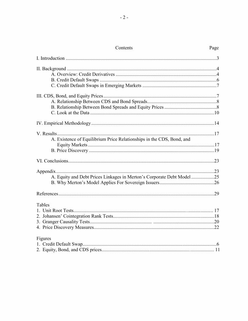
Contents Page

I. Introduction ............................................................................................................................3

II. Background ...........................................................................................................................4 A. Overview: Credit Derivatives ...................................................................................4 B. Credit Default Swaps ................................................................................................6 C. Credit Default Swaps in Emerging Markets .............................................................7

III. CDS, Bond, and Equity Prices .............................................................................................7 A. Relationship Between CDS and Bond Spreads.........................................................8 B. Relationship Between Bond Spreads and Equity Prices ...........................................8 C. Look at the Data ......................................................................................................10

IV. Empirical Methodology.....................................................................................................14

V. Results.................................................................................................................................17 A. Existence of Equilibrium Price Relationships in the CDS, Bond, and Equity Markets ........................................................................................................17 B. Price Discovery .......................................................................................................19

VI. Conclusions........................................................................................................................23

Appendix..................................................................................................................................23 A. Equity and Debt Prices Linkages in Merton’s Corporate Debt Model ...................25 B. Why Merton’s Model Applies For Sovereign Issuers.............................................26

References................................................................................................................................29 Tables 1. Unit Root Tests................................................................................................................... 17 2. Johansen’ Cointegration Rank Tests...................................................................................18 3. Granger Causality Tests................................................... ..................................................20 4. Price Discovery Measures...................................................................................................22 Figures 1. Credit Default Swap.................................................................................. ............................6 2. Equity, Bond, and CDS prices............................................................................................. 11

- 3 -

I. INTRODUCTION

In the past few years, the credit derivatives market has grown rapidly. According to a recent survey conducted by the British Bankers’ Association, the credit derivatives market has expanded from US$1.8 billion in 1993 to US$2.0 trillion in 2002. This survey further estimates that the total outstanding value will reach US$4.8 trillion by 2004. The rapid expansion of credit derivatives, in particular, the credit default swap market, has fostered greater interlinkages in the financial markets and greater interaction between different asset classes.

Credit derivatives are financial instruments that allow credit risk to be traded from one party to another party without actually transferring the ownership of the underlying assets. 2 These instruments strip out and isolate credit risk from other factors such as market risk.3 Therefore, it is believed that they provide more efficient allocation and pricing of credit risk than other credit-related instruments. Credit derivatives products are created by combining various financing strategies such as swap contracts or pooled securities. These products address credit risk embedded in underlying assets, and they provide insurance-like protection from the credit risk or default risk. The rapid development of credit derivatives, in particular of the credit default swap (CDS) market, offers an opportunity to gauge market views on a firm or bond issuer’s credit risk. The changes in a firm’s credit risk not only affect credit derivatives prices written on the firm, but they also affect the firm’s equity and bond prices. For example, when a firm is in a distressed condition, its credit risk or default risk increases. Thus, the price of bonds issued by the firm, and similarly, the firm’s share price would fall. When firms are in this situation, buying insurance against their default becomes more expensive. Therefore, the credit default price (spread) would rise. Also, the demand for protection against the firm’s potential default increases as credit risk increases. This in turn causes further downward pressure on bond and equity prices as sellers of credit derivative protection hedge their exposure by either shorting bonds, or the firm’s equity. The academic literature on the relationship between credit derivatives, bond, and equity markets is very small. However, the following authors provide some insight. Duffie (1999) and Hull and White (2000) suggest that in the absence of market friction the arbitrage forces CDS spreads to be approximately equal to the underlying bond spreads, and the CDS and bond spreads are positively correlated. The relationship between equity and bond markets is provided by Merton (1974). In his model, Merton notes that the firm’s liabilities constitute a barrier point for the

2 Underlying assets may be bank loans or commercial bonds. Or it could be other financial obligations on which the cash flows and/or credit event for credit derivatives are based.

3 Credit risk is a risk that the counterparties to transactions will fail to make obligated payments. Credit risk is sometimes called default risk. Market risk refers to movements in interest rates, exchange rates, stock prices, or commodity prices.

- 4 -

value of its assets. Within this framework, he notes that if the value of a firm’s assets falls below the face value of its debt, the firm would default. And hence, when debt to asset ratios are high, or when default risk is high, equity and bond prices are positively correlated, and vice versa. These theories also suggest that prices in the CDS, bond, and equity markets adjust simultaneously when there is new information on credit risk. That is, the revelation of new information, or price discovery, occurs in all three markets at the same time. Market practitioners claim, however, that the CDS market reacts first to new information on credit risk. Recent empirical studies appear to validate this claim for corporate issuers in Europe and the United States. For instance, Hull, Predescu, and White (2003) and Blanco, Brennan, and Marsh (2003) analyzed a large panel of U.S. and European corporate issuers and found that CDS spreads lead bond spreads during credit deterioration episodes. Blanco, Brennan, and Marsh (2003) also found evidence supporting the existence of an equilibrium relationship between CDS and bond spreads for a sample of U.S. and European firms. Longstaff, Mithal, and Neiss (2003) have studied a large sample of corporate issuers in the United States and found that the information in the CDS and equity markets leads information in the bond market. What implications can we find for emerging market sovereign issuers? This paper addresses this question and examines the equilibrium price relationships and price discovery in the CDS, bond, and equity markets for the following eight emerging market countries: Brazil, Bulgaria, Colombia, Mexico, the Philippines, Russia, Turkey, and Venezuela. This study also attempts to extend Merton’s theory of the firm to sovereign issuers. We provide our justification in the appendix. The remainder of the paper is organized as follows. Section II provides a brief overview of the credit derivatives market and credit default swaps. Section III describes the theoretical relationship between CDS, bonds, and equities in more detail. Section IV presents our empirical studies. Section V concludes the paper.

II. BACKGROUND

This section provides a brief overview of the credit derivatives market and, in particular, of credit default swaps. Most credit derivatives market activity relates to mature market issuers, and emerging market issuers comprise only a small share of total market activity. In the past few years, however, emerging market credit derivatives have evolved rapidly, and CDS has become a dominant product in the emerging market structured credit market.

A. Overview: Credit Derivatives

Credit derivatives are financial contracts that allow credit risk to be transferred from one party to another against credit-related losses. As products, credit derivatives combine two key developments in the financial markets: derivatives and securitization. Most of all, these products are designed to isolate credit risk from other sources of risk such as market risk. Therefore, they allow credit risk to be transferred at a relatively low cost.

- 5 -

Credit derivatives have evolved rapidly in the past few years. In particular, increased standardization of contracts, according to International Swap Dealers Association (ISDA) Credit Derivatives Definitions, has removed some of the legal obstacles to the development of the market. It has also prompted increased trading through brokers (GFINet, CreditTrade). In the case of CDS, contracts offered by different market makers have become almost identical, allowing end-users to shop for the best price.4 These developments have facilitated investment and hedging opportunities not readily available in the cash market, and have helped to increase leverage, reduce funding costs, and economize regulatory capital.

According to a British Bankers’ Association (BBA) Survey, the credit derivatives market was about $2.0 trillion in 2002. In 1997, the total global value was $180 billion. This market is estimated to grow to $4.8 trillion by the end of 2004. The credit derivatives market is relatively small compared with other derivatives markets, but it is one of the fastest growing segments in the global over-the-counter derivatives market. The main players in this market are banks, securities houses, hedge funds, and insurance companies. Banks are the biggest buyers and sellers of protection. Insurance companies come second to banks as sellers of protection, followed by securities houses and hedge funds.5 At the moment, only the more sophisticated financial institutions and corporations use credit derivatives because of the complexities involved in dealing with event monitoring, counterparty exposure, and pricing the instruments.

Broadly, there are four types of credit derivatives: total return swaps, credit default swaps (CDSs), credit linked notes, and synthetic collateralized debt obligations (CDO). 6 A total return swap is an agreement to exchange the total return on a bond or other reference asset for LIBOR plus a spread. A CDS is a swap in which one party makes payments only if a specified credit event (or events) occurs. Credit linked notes are a securitized form of credit derivatives. Finally, a synthetic CDO is an asset-backed security whose collateral is typically a portfolio of bonds or bank loans.

4 It should be noted here that in the United States restructuring is accepted as a credit event while it is not accepted in Europe. Therefore, sometimes, the U.S. contract may not be substitutable for European contract.

5 In September 2003, banks sold US$1.3 trillion of gross credit protection though they were net buyers of protection in the amount of US$229 billion. Insurance companies sold protection in a net amount of US$303 billion (FitchRatings, 2003).

6 For more information on these instruments, see Tavakoli (1998).

- 6 -

B. Credit Default Swaps

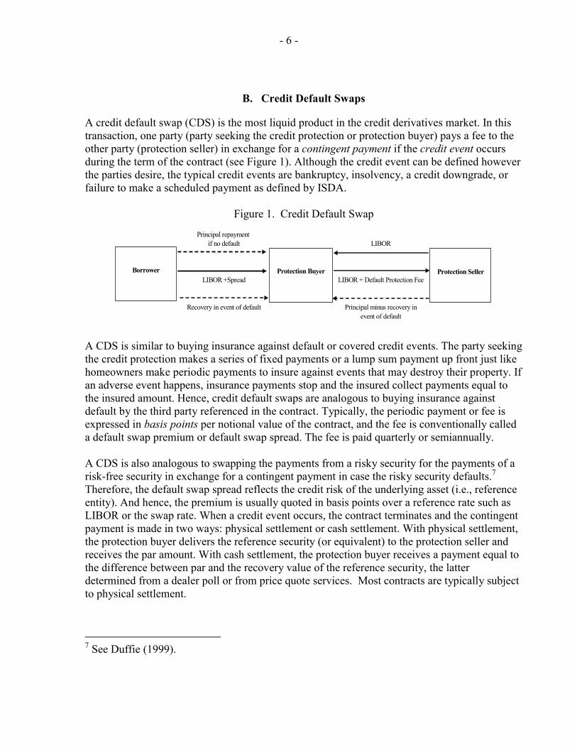
A credit default swap (CDS) is the most liquid product in the credit derivatives market. In this transaction, one party (party seeking the credit protection or protection buyer) pays a fee to the other party (protection seller) in exchange for a contingent payment if the credit event occurs during the term of the contract (see Figure 1). Although the credit event can be defined however the parties desire, the typical credit events are bankruptcy, insolvency, a credit downgrade, or failure to make a scheduled payment as defined by ISDA.

Figure 1. Credit Default Swap

Principal repayment if no default

LIBOR +Spread

Recovery in event of default Principal minus recovery inevent of default

LIBOR + Default Protection Fee

LIBOR

Borrower Protection Buyer Protection Seller

A CDS is similar to buying insurance against default or covered credit events. The party seeking the credit protection makes a series of fixed payments or a lump sum payment up front just like homeowners make periodic payments to insure against events that may destroy their property. If an adverse event happens, insurance payments stop and the insured collect payments equal to the insured amount. Hence, credit default swaps are analogous to buying insurance against default by the third party referenced in the contract. Typically, the periodic payment or fee is expressed in basis points per notional value of the contract, and the fee is conventionally called a default swap premium or default swap spread. The fee is paid quarterly or semiannually. A CDS is also analogous to swapping the payments from a risky security for the payments of a risk-free security in exchange for a contingent payment in case the risky security defaults.7 Therefore, the default swap spread reflects the credit risk of the underlying asset (i.e., reference entity). And hence, the premium is usually quoted in basis points over a reference rate such as LIBOR or the swap rate. When a credit event occurs, the contract terminates and the contingent payment is made in two ways: physical settlement or cash settlement. With physical settlement, the protection buyer delivers the reference security (or equivalent) to the protection seller and receives the par amount. With cash settlement, the protection buyer receives a payment equal to the difference between par and the recovery value of the reference security, the latter determined from a dealer poll or from price quote services. Most contracts are typically subject to physical settlement.

7 See Duffie (1999).

- 7 -

Finally, CDSs are actively traded on corporate, bank, and sovereign debt, and the usual contract is written on notional amounts of US$5 million and US$10 million with a five-year maturity.8 Most of the contracts are drawn to reference bonds by a single issuer, that is single name contracts. When contracts refer to multiple issuers, they are referred to as portfolio names. The most popular portfolio transaction is probably the first-to-default swap basket. In these contracts, protection is sold on a basket of credit default swaps. Payments are terminated when the first credit event happens or after a fixed period of time.

C. Credit Default Swaps in Emerging Markets

With regard to emerging markets, most contracts traded in the credit derivatives markets reference sovereign issuers. Therefore, trading in single name sovereigns is more liquid than in corporate names. According to Deutsche Bank, the notional amounts outstanding in emerging market credit derivatives in 2002 was US$300 billion, roughly equal to 15 percent of the market.9 In emerging markets, standard maturities are 1, 2, 3, 5, and 10 years. In general, the liquidity of sovereign CDSs depends on the liquidity of sovereign bonds. Thus for countries with very liquid bond markets such as Mexico, Brazil, Colombia, and Venezuela, it is rather easy to find both CDS bid and ask price quotes. The absence of significant trading in contracts referenced to emerging market corporate issuers reflects both the scarcity of corporate debt issued in foreign currencies and the illiquidity of emerging market corporate bonds.

Major players in the emerging market CDSs are hedge funds, emerging market dedicated mutual funds, pension funds, and banks. Hedge funds use CDSs actively either for taking directional bets on the future creditworthiness of a country or to arbitrage the spread differential between the CDS and the referenced bond. Pension funds and emerging market dedicated mutual funds use CDSs to manage their exposure to emerging market sovereign bonds. Similarly, banks use CDSs to manage their balance sheet exposure to emerging market borrowers.

III. CDS, BOND, AND EQUITY PRICES

In this section, we discuss price dynamics in the CDS, bond, and equity markets. Our discussion is largely based on the theories proposed by Duffie (1999), Hull and White (2000), and Merton (1974).

8 Although a large number of contracts are written on 5-year maturity, investment banks also write CDS contracts on the notional amounts and maturities specified by their clients. For corporate and financial institutions, however, trading activity is greatest for five-year contracts.

9 See Xu (2003).

- 8 -

A. Relationship Between CDS and Bond Spreads

An investor who owns a risky bond can protect himself against default (credit) risk by buying the corresponding CDS. Ruling out arbitrage, this strategy requires that CDS and bond spreads are the same. The intuition is as follows. Suppose we buy a risky bond (e.g., corporate bond) that pays a risk-free rate plus a constant spread. Suppose we also buy a CDS on this risky bond to insure against possible default. This transaction would yield a return equal to the risk-free rate plus the CDS and bond spread differential, or default swap basis. However, since these two transactions are equivalent to holding a risk-free bond (e.g., treasury), they should yield a return that is equal to the risk-free rate. Therefore, there should be no spread differential between CDSs and bonds. Duffie (1999) and Hull and White (2000) formalize this argument and explain what specialized assumptions are needed for it to hold true. In terms of price dynamics, theory suggests that there should be one-to-one changes between CDS and bond spreads. 10 In practice, however, various factors can cause CDS and bond spreads to be different. First, CDS and bond spreads can diverge because of the “cheapest-to-deliver” option in the CDS contract. When the credit event occurs, this option allows buyers of a CDS to deliver a bond that is the cheapest—in other words, one that is worth less than the one referenced in the contract. In this case, the seller of a CDS (the one who receives the fee) would then face a bigger loss than originally anticipated because the bond that is delivered is worth less than the bond the contract was written on. Consequently, the seller charges a CDS spread that is higher than the bond spread. The excess spread is a cheapest-to-deliver premium. This may cause the spread differentials between CDS and bond to widen. However, this premium should be stable over time since the number of bonds available for delivery remains the same over an extended period.

Another factor that may cause the CDS and bond spreads to be different is relative liquidity in the CDS and/or bond markets. In the case of sovereign issuers, bond markets are more liquid that CDS markets. So, the CDS would trade at a higher spread than the referenced bond to compensate investors for lower liquidity. If the relative liquidity of the CDS and bond markets remains unchanged, the spread differential between CDS and bonds should remain stable. This is the case most of the time. However, there are instances in which liquidity may migrate from one market to the other, causing CDS and bond spreads to diverge.

B. Relationship Between Bond Spreads and Equity Prices

Merton (1974) formalizes the relationship between bond and equity prices using option-pricing theory. He says that equity is analogous to a call option when the firm is also financed by debt.

10 The main assumptions are: first, the risky bond and the risk-free bond are par-floating rate securities. Second, there are no transaction costs, and tax effects are negligible. Third, the payment of the CDS spread stops if a credit event occurs. Finally, protection buyers are paid on the next coupon date following the occurrence of the credit event.

- 9 -

Equity holders can own the assets of the firm only after paying back the face value of debt to creditors. If the assets of the firm are worth more than its debt, the call option is “in-the-money.” Otherwise, equity is worthless, and the call option is “out-of-the-money.”

From Merton’s model, we can gain further insight about the relationship between bond and equity prices. Merton’s model is based on the capital structure of the firm, that is, it takes a balance sheet approach to examining the relationship between equity and debt. In this framework, he notes that a firm’s liabilities constitute a barrier point for the value of its assets. Thus, if the value of a firm’s assets falls below the face value of its debt, the firm would default.

Merton also notes that bond and equity prices are positively correlated, and that the correlation is stronger when debt to asset ratios are high, or when default risk is high. If the firm’s value is just enough to cover the face value of its debt, then relatively small changes in firm value could cause it to default. But the negative movement in the firm value are not only reflected in declining equity prices but also in declining bond prices. Typical firms fitting this bond-equity price patterns are those with high debt-to-equity ratios and below investment-grade ratings. This tells us that when default risk is a major concern, equity prices and bond spreads move in opposite directions.

From this result and the one earlier on the CDSs and bonds, we infer that the price relationship between CDS spreads and equity prices has to be opposite. But in order for us to examine this relationship for the emerging market countries, we must first find out if we can extend Merton’s theory to the sovereigns. While it is easy to speculate on this argument, applying Merton’s theory of the firm to the sovereign issuers poses a challenge because the sovereign issuers may choose to default even when it is technically solvent. In the appendix, we explain how Merton’s model can be extended to accommodate this problem.

Briefly, we extend the original Merton’s theory of firm to sovereigns by noting that there are two critical asset values. These two points are “default value” and “no-payment value.” For corporate issuers, the “no-payment value” and the “default value” are zero and the face value of debt, respectively. For sovereigns, however, the “willingness-to-pay factor” implies that “default value” is greater than face value of debt and “no-payment value” is greater than zero. Hence, for sovereigns, “willingness to pay” implies that the corresponding values are higher. That is, when the country defaults or ceases debt payments, its assets are worth more than its debt and the country’s asset value is still positive. Therefore, the only substantial difference between a corporate and a sovereign issuer with the same amount of debt is that default risk is higher for the sovereign for every asset value. Thus, the relationship between debt and equity prices should remain the same between the corporate and sovereigns issuers. For more details, see appendix.

- 10 -

C. Look at the Data

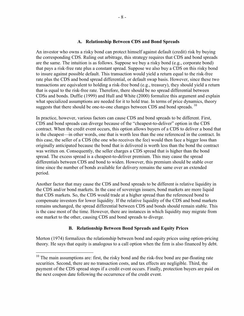
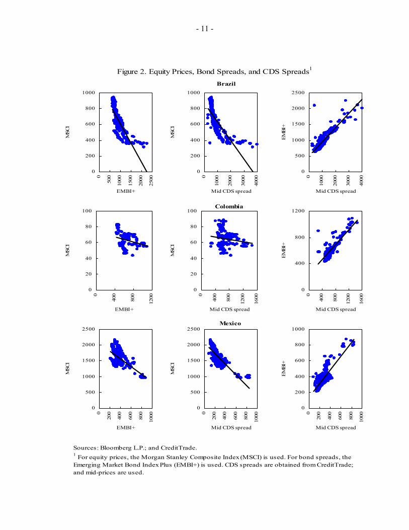
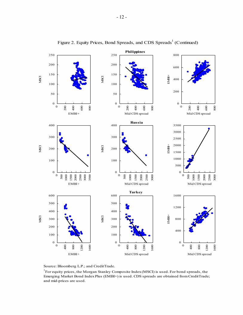
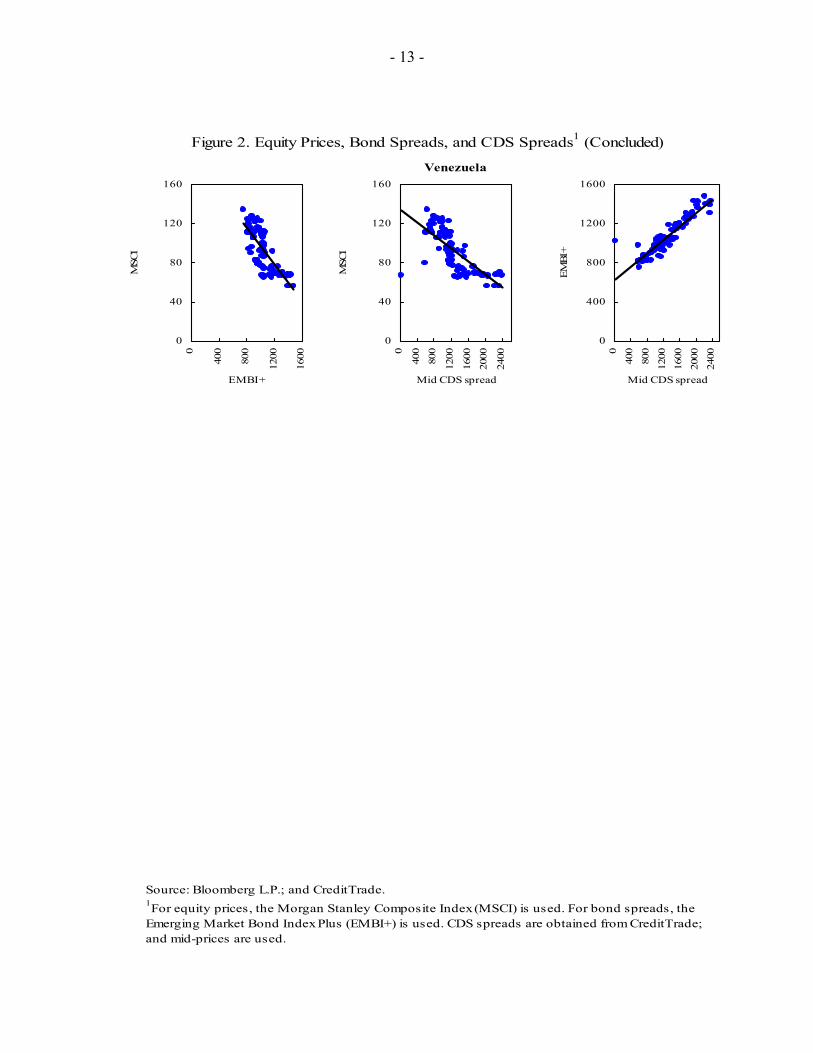
Before we present our empirical analysis, we plot the data to explore if we could gain any insight into the relationship between CDS, bond, and equity prices. The following countries are reviewed: Brazil, Bulgaria, Colombia, Mexico, the Philippines, Russia, Turkey, and Venezuela. These countries have foreign currency–denominated external debt that are below investment grade except Mexico which has been rated investment–grade since March 2002. The CDS, bond, and equity data are daily data for the period March 19, 2001 through May 29, 2003. For purposes of cross-country comparisons, we use country bond and equity indexes. The CDS spreads are mid-price quotes on five-year contracts obtained from CreditTrade and Deutsche Bank. We use CreditTrade data to plot the chart, but for empirical analysis we use Deutsche Bank data because CreditTrade data are not always continuous. The bond spreads correspond to the JP Morgan Chase Emerging Market Bond Index Plus (EMBI+). The equity prices are obtained from the U.S. dollar-denominated Morgan Stanley Capital Equity Price Indices (MSCI). We use MSCI indices as a proxy for the equity value of the country. Figure 2 shows the graph of CDS, bond, and equity prices. In column (1), the bond spreads and equity prices are shown. Most countries exhibit inverse relationship between these two markets. In column (2), we find that CDS spreads and equity prices are negatively correlated. As anticipated, these correlation patterns strongly reflect the price relationships that we noted earlier in the theory section. In column (3), we plot the CDS spreads and bond spreads. Here, again, we find that most countries have positive correlation between these two markets. Next, we present a more formal empirical analysis.

- 11 -

Figure 2. Equity Prices, Bond Spreads, and CDS Spreads1

Sources: Bloomberg L.P.; and CreditTrade.1 For equity prices, the Morgan Stanley Composite Index (MSCI) is used. For bond spreads, the Emerging Market Bond Index Plus (EMBI+) is used. CDS spreads are obtained from CreditTrade; and mid-prices are used.

0

200

400

600

800

10000

500

1000

1500

2000

2500

EMBI+

MSC

I

0

200

400

600

800

1000

0

1000

2000

3000

4000

Mid CDS spread

MSC

I0

500

1000

1500

2000

2500

0

1000

2000

3000

4000

Mid CDS spread

EMBI

+0

20

40

60

80

100

0

400

800

1200

EMBI+

MSC

I

0

20

40

60

80

100

0

400

800

1200

1600

Mid CDS spread

MSC

I

0

400

800

1200

0

400

800

1200

1600

Mid CDS spread

EMBI

+

0

500

1000

1500

2000

2500

0

200

400

600

800

1000

EMBI+

MSC

I

0

500

1000

1500

2000

2500

0

200

400

600

800

1000

Mid CDS spread

MSC

I

0

200

400

600

800

1000

0

200

400

600

800

1000

Mid CDS spread

EMBI

+

Brazil

Colombia

Mexico

- 12 -

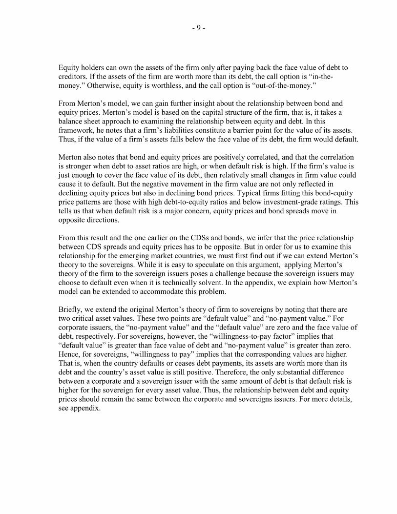
Figure 2. Equity Prices, Bond Spreads, and CDS Spreads1 (Continued)

Source: Bloomberg L.P.; and CreditTrade.1For equity prices, the Morgan Stanley Composite Index (MSCI) is used. For bond spreads, the Emerging Market Bond Index Plus (EMBI+) is used. CDS spreads are obtained from CreditTrade; and mid-prices are used.

0

50

100

150

200

2500

200

400

600

800

EMBI+

MSC

I

0

50

100

150

200

250

0

200

400

600

800

Mid CDS spread

MSC

I0

200

400

600

800

0

200

400

600

800

Mid CDS spread

EMBI

+0

100

200

300

400

0

500

1000

1500

2000

2500

3000

3500

EMBI+

MSC

I

0

100

200

300

400

0

500

1000

1500

2000

2500

3000

Mid CDS spread

MSC

I

0

500

1000

1500

2000

2500

3000

3500

0

500

1000

1500

2000

2500

3000

Mid CDS spread

EMBI

+

0

100

200

300

400

500

600

0

400

800

1200

1600

EMBI+

MSC

I

0

100

200

300

400

500

600

0

400

800

1200

1600

Mid CDS spread

MSC

I

0

400

800

1200

1600

0

400

800

1200

1600

Mid CDS spread

EMBI

+

Philippines

Russia

Turkey

- 13 -

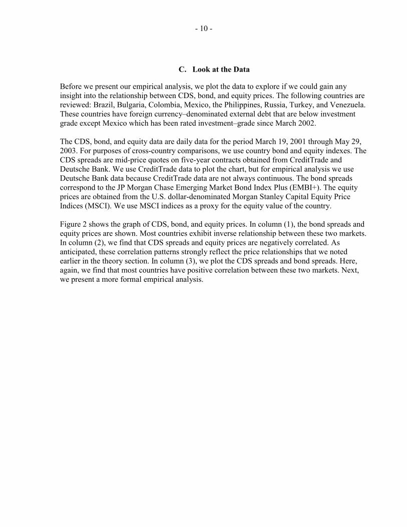
Figure 2. Equity Prices, Bond Spreads, and CDS Spreads1 (Concluded)

Source: Bloomberg L.P.; and CreditTrade.1For equity prices, the Morgan Stanley Composite Index (MSCI) is used. For bond spreads, the Emerging Market Bond Index Plus (EMBI+) is used. CDS spreads are obtained from CreditTrade; and mid-prices are used.

0

40

80

120

1600

400

800

1200

1600

EMBI+

MSC

I

0

40

80

120

160

0

400

800

1200

1600

2000

2400

Mid CDS spread

MSC

I0

400

800

1200

1600

0

400

800

1200

1600

2000

2400

Mid CDS spread

EMBI

+

Venezuela

- 14 -

IV. EMPIRICAL METHODOLOGY

In order to test the equilibrium price relationship and price discovery between CDS, bond, and equity markets, we use cointegration analysis, Granger causality tests, and the price discovery measures proposed by Hasbrouck (1995) and Gonzalo and Granger (1995). Our analysis is conducted in two steps. First, we test for the existence of the price equilibrium, using cointegration analysis through a two-step approach. The two-step approach consists of i) testing if the price series are stationary or have unit roots, and ii) using the cointegration rank test proposed by Johansen (1991). Second, we analyze price discovery measures using Granger causality tests and the methods proposed by Hasbrouck and Gonzalo and Granger. Figure 2 suggests the equilibrium price relationship between any two markets is linear. The standard technique for analyzing linear relationships between two variables is ordinary least squares (OLS). However, Granger and Newbold (1974) showed that this technique is inadequate when the variables are characterized by a unit root. That is, the variables drift away from their initial value without following any specific trend. In this case, Granger and Newbold note that OLS would falsely suggest that the variables are closely connected by a linear equation even though they are completely independent of each other.

Cointegration analysis addresses such shortcomings of OLS. Therefore, we use cointegration analysis to determine whether there is an equilibrium price relationship between two markets. If there is an equilibrium relationship between the variables, there is a linear combination of the variables that is stationary. That is, the values of the linear combination of the variables are centered around a mean value and have constant variance. When we have this condition, we say that the variables are cointegrated and the coefficients of the linear combination are referred to as cointegrating vector. Therefore, testing for the existence of an equilibrium price relationship is equivalent to testing for the existence of a cointegrating equation.

We test for the existence of equilibrium price relationships or cointegrating equations, using a two-step approach. First, we determine whether the price series are characterized by a unit root using Augmented Dickey-Fuller and Phillips-Perron unit root test. The null hypothesis in both tests is that the series are characterized by unit root tests. The Augmented Dickey-Fuller test for a series y is carried out using the following regression equation:

1 1 1 2 2 ...t t t t p t p ty y y y y eα β ς ς ς− − − −∆ = + + ∆ + ∆ + + ∆ + , (1) where ∆ is the first difference operator, p is the number of lags, and e is an error term. The inclusion of lagged first-differenced variables in the regression controls for higher order correlation in the series. The null hypothesis is that β = 0, and it implies that y is characterized by a unit root. The Phillips-Perron test is based on the following regression: 1t t ty y eα β −∆ = + + . (2)

- 15 -

Again, the null hypothesis is β = 0, and it implies that y is characterized by a unit root. In the Phillips-Perron test, the Newey-West procedure is used to correct for the higher order correlation of the error term rather than the Augumented Dickey-Fuller test. When two price series are characterized by unit roots, we use cointegration rank test as proposed by Johansen (1991) to test for the existence of a price equilibrium relationship. The cointegration rank test is performed on a vector autoregression of order p: 1 1 ...t t p t p tY AY A Y ε− −= + + + , (3) where Y is a 2×1 vector of prices. The vector autoregression can be rewritten as:

1

11

p

t t i t i ti

Y Y Y e−

− −=

∆ = Π + Γ ∆ +∑ , (4)

where 1

p

ii

A I=

Π = −∑ , and 1

p

i jj i

A= +

Γ = −∑ .

If the two price series are cointegrated, coefficient matrix Π has reduced rank equal to 1, and there exist 2×1 vectors α and β such that Π = α βT, where the vector β is the cointegrating vector. Johansen’s cointegration rank tests evaluate the null hypothesis of no cointegration. This null hypothesis states that the coefficient matrix has full rank equal to 2. If this null hypothesis is rejected, then the two price series are cointegrated and we can affirm that there exists an equilibrium price relationship between them. For price discovery, the following tests are used: Granger causality, Hasbrouck (1995) and Gonzalo and Granger (1995). Granger causality tests are the simplest way to test whether one market has a dominant role in price discovery. Given two series x and y, we say that series x Granger causes series y if past values of x contain useful information beyond that contained in past values of y to explain the current value of y. Since we need to determine the price discovery between CDS, bond, and equity markets, we implement this test on these markets on all possible pairwise combinations using the following regression form:

,11

1 ∑∑=

−=

− ∆+∆+=∆n

jjtj

n

jjtjt xbyacy (5)

where n is the number of lags, 1c is a constant, ∆ is the first difference operator, and the coefficients associated with the lagged values of series y and x are aj and bj, j = 1,..,n, respectively. In the context of equation (5), the null hypothesis is that x does not Granger-causes y, implying the joint hypothesis that bj =0, j = 1,..,n. In other words, when analyzing market Y, the null hypothesis is that there is no price discovery in market X since prices there cannot explain current prices in market Y. Theory suggests two-way Granger causation: x Granger- causes y and y Grange-causes x for every single pairwise combination of markets. That is, price

- 16 -

discovery occurs in both markets. In our analysis, Granger causality tests were performed for 1, 5, 10, and 20 business day lags, so that price discovery up to a one-month horizon could be tested for each market combination. Next, we use two additional measures to determine each individual market contribution in the price discovery process.11 These two measures are Hasbrouck (1995) and Gonzalo and Granger (1995). These methods assume that the variables analyzed are cointegrated, and they are based on a vector error-correction model (VECM) formulation:

11

'k

t t j t j tj

Y Y A Y eαβ − −=

∆ = + ∆ +∑ , (6)

where Y is the vector of endogenous variables, α is the error correction vector, β is the cointegrating vector, and e is a serially uncorrelated zero-mean error term with covariance matrix Ω. The Hasbrouck (1995) measure is derived from the vector moving average representation (VMA) of equation (3):

*

1

(1) ( )t

t j tj

Y e L e=

= Ψ +Ψ∑ , (7)

where Ψ and Ψ* are matrix polynomials in the lag operator L. Given a vector of shocks in period t, et, Ψ(1) et measures the long-run impact of the shocks. Hasbrouck noted that, in a bivariate system, the rows of the long-run impact matrix Ψ(1) are identical if the cointegrating vector β is (1, –1). In this case, the term Ψ(1) et is equivalent to a common trend, and lower and upper bounds to the price discovery contribution of each variable can be determined from its contribution to the total variance of the common trend component. If the cointegrating vector is not equal to (1,–1), lower and upper bounds for the contribution of each market to price discovery can still be determined from the Cholesky decomposition of the long-run impact matrix Ψ(1). Gonzalo and Granger (1995) methodology is derived from the finding of Stock and Watson (1991) that a cointegrated system admits a common factor representation of the form: t t tY f G= + , (8) where f is a common factor and G is a stationary component. Gonzalo and Granger showed that, if the common factor is a linear combination of the system variables, it can be expressed as

11 The interested reader should refer to the original citations, Baillie and others (2002), and Lehman (2002). See Blanco, Brennan, and Marsh (2003) for an application to CDS and bond spreads at the corporate level,

- 17 -

t tf Yα⊥= , where α⊥ is a vector orthogonal to the error-correction vector α. The contribution of each variable is directly proportional to its relative weight in determining the common vector; that is, it can be measured by the GG statistics /i iα α⊥ ⊥∑ , i=1,..,n. Hasbrouck and Gonzalo and Granger price discovery measures are calculated after estimating the bivariate VECM of equation (6) for each pair of market combination. The lag selection in the VECM are based on the Schwarz information criterion (SIC) rather than the conventional Aikake information criterion (AIC), as suggested by Hayashi (2000). Finally, we analyze the error-correction coefficients in equation (6) for additional information on the price discovery process. Equation (6) is a bivariate system of equations. In each equation, there is an error-correction coefficient that measures how much prices in that market need to adjust as prices deviate from their equilibrium price relationship. If price discovery happens only in one market, then its related error-correction coefficient is statistically insignificant. If price discovery happens in both markets, however, then the error-correlation coefficient in both markets should be statistically significant.

V. RESULTS

A. Existence of Equilibrium Price Relationships in the CDS, Bond, and Equity Markets

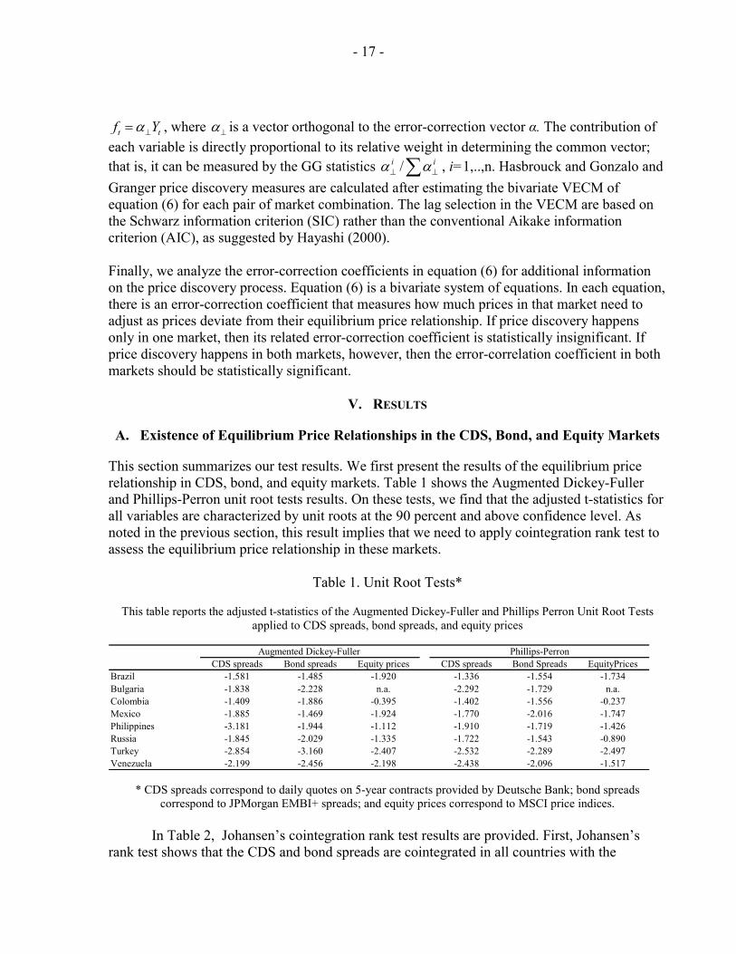
This section summarizes our test results. We first present the results of the equilibrium price relationship in CDS, bond, and equity markets. Table 1 shows the Augmented Dickey-Fuller and Phillips-Perron unit root tests results. On these tests, we find that the adjusted t-statistics for all variables are characterized by unit roots at the 90 percent and above confidence level. As noted in the previous section, this result implies that we need to apply cointegration rank test to assess the equilibrium price relationship in these markets.

Table 1. Unit Root Tests*

This table reports the adjusted t-statistics of the Augmented Dickey-Fuller and Phillips Perron Unit Root Tests applied to CDS spreads, bond spreads, and equity prices

CDS spreads Bond spreads Equity prices CDS spreads Bond Spreads EquityPricesBrazil -1.581 -1.485 -1.920 -1.336 -1.554 -1.734Bulgaria -1.838 -2.228 n.a. -2.292 -1.729 n.a.Colombia -1.409 -1.886 -0.395 -1.402 -1.556 -0.237Mexico -1.885 -1.469 -1.924 -1.770 -2.016 -1.747Philippines -3.181 -1.944 -1.112 -1.910 -1.719 -1.426Russia -1.845 -2.029 -1.335 -1.722 -1.543 -0.890Turkey -2.854 -3.160 -2.407 -2.532 -2.289 -2.497Venezuela -2.199 -2.456 -2.198 -2.438 -2.096 -1.517

Augmented Dickey-Fuller Phillips-Perron

* CDS spreads correspond to daily quotes on 5-year contracts provided by Deutsche Bank; bond spreads

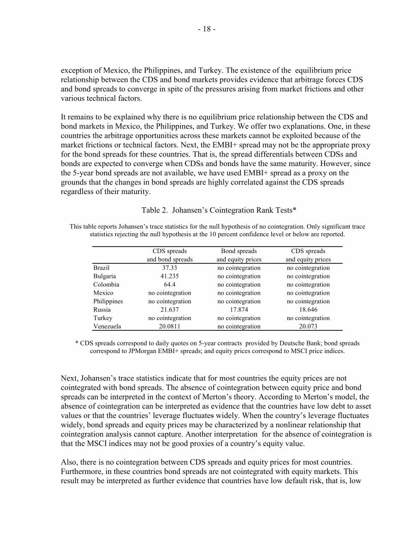
correspond to JPMorgan EMBI+ spreads; and equity prices correspond to MSCI price indices. In Table 2, Johansen’s cointegration rank test results are provided. First, Johansen’s

rank test shows that the CDS and bond spreads are cointegrated in all countries with the

- 18 -

exception of Mexico, the Philippines, and Turkey. The existence of the equilibrium price relationship between the CDS and bond markets provides evidence that arbitrage forces CDS and bond spreads to converge in spite of the pressures arising from market frictions and other various technical factors. It remains to be explained why there is no equilibrium price relationship between the CDS and bond markets in Mexico, the Philippines, and Turkey. We offer two explanations. One, in these countries the arbitrage opportunities across these markets cannot be exploited because of the market frictions or technical factors. Next, the EMBI+ spread may not be the appropriate proxy for the bond spreads for these countries. That is, the spread differentials between CDSs and bonds are expected to converge when CDSs and bonds have the same maturity. However, since the 5-year bond spreads are not available, we have used EMBI+ spread as a proxy on the grounds that the changes in bond spreads are highly correlated against the CDS spreads regardless of their maturity.

Table 2. Johansen’s Cointegration Rank Tests*

This table reports Johansen’s trace statistics for the null hypothesis of no cointegration. Only significant trace statistics rejecting the null hypothesis at the 10 percent confidence level or below are reported.

CDS spreads Bond spreads CDS spreadsand bond spreads and equity prices and equity prices

Brazil 37.33 no cointegration no cointegrationBulgaria 41.235 no cointegration no cointegrationColombia 64.4 no cointegration no cointegrationMexico no cointegration no cointegration no cointegrationPhilippines no cointegration no cointegration no cointegrationRussia 21.637 17.874 18.646Turkey no cointegration no cointegration no cointegrationVenezuela 20.0811 no cointegration 20.073

* CDS spreads correspond to daily quotes on 5-year contracts provided by Deutsche Bank; bond spreads

correspond to JPMorgan EMBI+ spreads; and equity prices correspond to MSCI price indices.

Next, Johansen’s trace statistics indicate that for most countries the equity prices are not cointegrated with bond spreads. The absence of cointegration between equity price and bond spreads can be interpreted in the context of Merton’s theory. According to Merton’s model, the absence of cointegration can be interpreted as evidence that the countries have low debt to asset values or that the countries’ leverage fluctuates widely. When the country’s leverage fluctuates widely, bond spreads and equity prices may be characterized by a nonlinear relationship that cointegration analysis cannot capture. Another interpretation for the absence of cointegration is that the MSCI indices may not be good proxies of a country’s equity value.

Also, there is no cointegration between CDS spreads and equity prices for most countries. Furthermore, in these countries bond spreads are not cointegrated with equity markets. This result may be interpreted as further evidence that countries have low default risk, that is, low

- 19 -

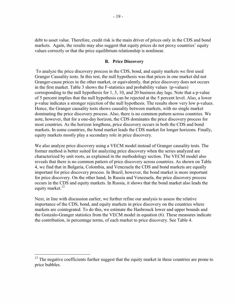
debt to asset value. Therefore, credit risk is the main driver of prices only in the CDS and bond markets. Again, the results may also suggest that equity prices do not proxy countries’ equity values correctly or that the price equilibrium relationship is nonlinear.

B. Price Discovery

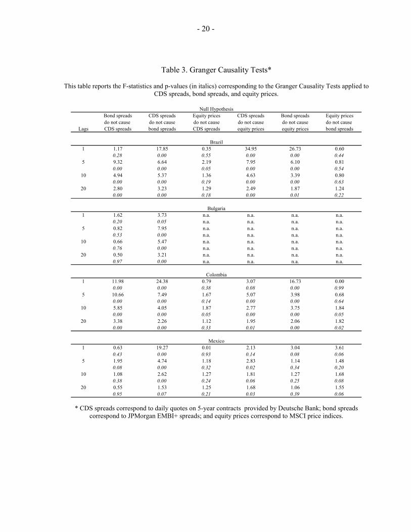
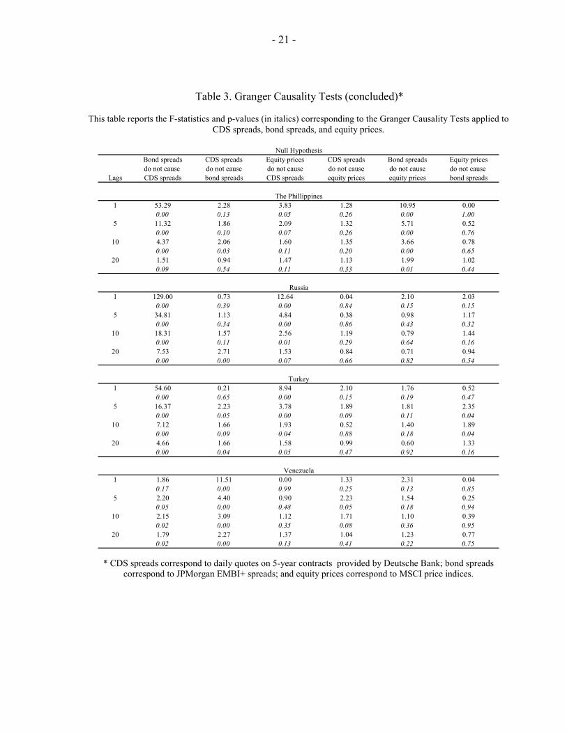
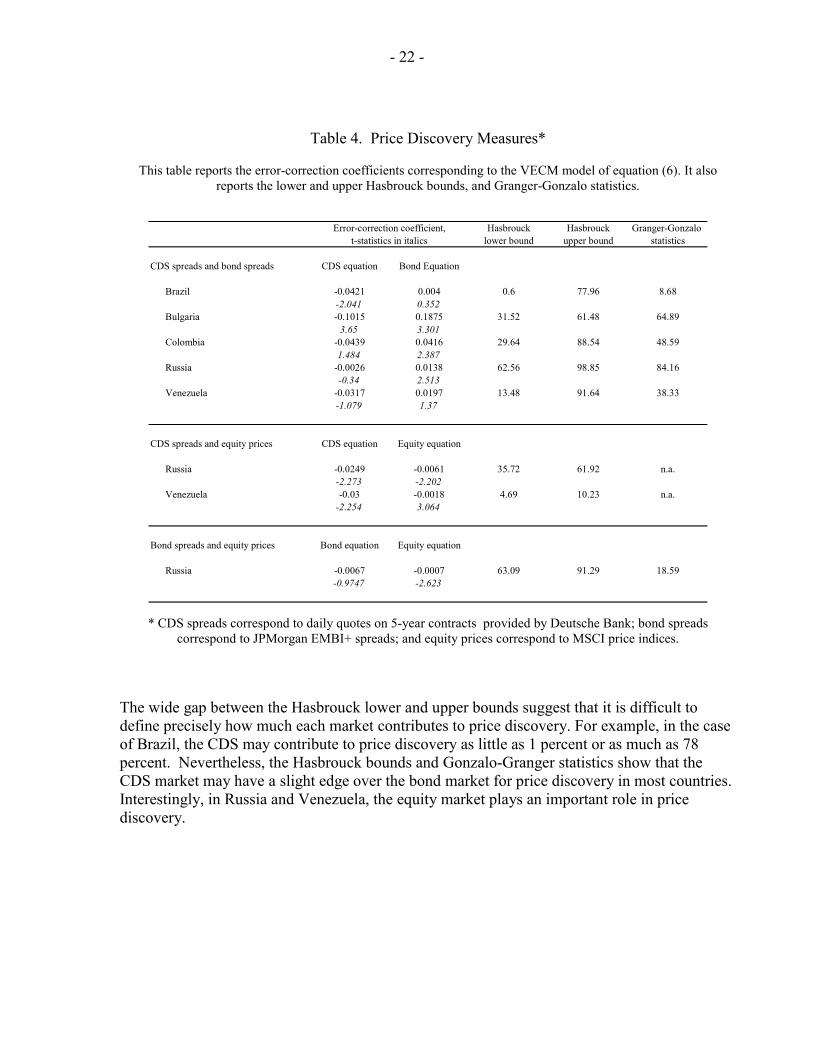
To analyze the price discovery process in the CDS, bond, and equity markets we first used Granger Causality tests. In this test, the null hypothesis was that prices in one market did not Granger-cause prices in the other market, or equivalently, that price discovery does not occurs in the first market. Table 3 shows the F-statistics and probability values (p-values) corresponding to the null hypothesis for 1, 5, 10, and 20 business day lags. Note that a p-value of 5 percent implies that the null hypothesis can be rejected at the 5 percent level. Also, a lower p-value indicates a stronger rejection of the null hypothesis. The results show very low p-values. Hence, the Granger causality tests shows causality between markets, with no single market dominating the price discovery process. Also, there is no common pattern across countries. We note, however, that for a one-day horizon, the CDS dominates the price discovery process for most countries. As the horizon lengthens, price discovery occurs in both the CDS and bond markets. In some countries, the bond market leads the CDS market for longer horizons. Finally, equity markets mostly play a secondary role in price discovery. We also analyze price discovery using a VECM model instead of Granger causality tests. The former method is better suited for analyzing price discovery when the series analyzed are characterized by unit roots, as explained in the methodology section. The VECM model also reveals that there is no common pattern of price discovery across countries. As shown on Table 4, we find that in Bulgaria, Colombia, and Venezuela the CDS and bond markets are equally important for price discovery process. In Brazil, however, the bond market is more important for price discovery. On the other hand, In Russia and Venezuela, the price discovery process occurs in the CDS and equity markets. In Russia, it shows that the bond market also leads the equity market.12

Next, in line with discussion earlier, we further refine our analysis to assess the relative importance of the CDS, bond, and equity markets in price discovery on the countries where markets are cointegrated. To do this, we estimate the Hasbrouck lower and upper bounds and the Gonzalo-Granger statistics from the VECM model in equation (6). These measures indicate the contribution, in percentage terms, of each market to price discovery. See Table 4.

12 The negative coefficients further suggest that the equity market in these countries are prone to price bubbles.

- 20 -

Table 3. Granger Causality Tests*

This table reports the F-statistics and p-values (in italics) corresponding to the Granger Causality Tests applied to CDS spreads, bond spreads, and equity prices.

Bond spreads CDS spreads Equity prices CDS spreads Bond spreads Equity pricesdo not cause do not cause do not cause do not cause do not cause do not cause

Lags CDS spreads bond spreads CDS spreads equity prices equity prices bond spreads

1 1.17 17.85 0.35 34.95 26.73 0.600.28 0.00 0.55 0.00 0.00 0.44

5 9.32 6.64 2.19 7.95 6.10 0.810.00 0.00 0.05 0.00 0.00 0.54

10 4.94 5.37 1.36 4.63 3.39 0.800.00 0.00 0.19 0.00 0.00 0.63

20 2.80 3.23 1.29 2.49 1.87 1.240.00 0.00 0.18 0.00 0.01 0.22

1 1.62 3.73 n.a. n.a. n.a. n.a.0.20 0.05 n.a. n.a. n.a. n.a.

5 0.82 7.95 n.a. n.a. n.a. n.a.0.53 0.00 n.a. n.a. n.a. n.a.

10 0.66 5.47 n.a. n.a. n.a. n.a.0.76 0.00 n.a. n.a. n.a. n.a.

20 0.50 3.21 n.a. n.a. n.a. n.a.0.97 0.00 n.a. n.a. n.a. n.a.

1 11.98 24.38 0.79 3.07 16.73 0.000.00 0.00 0.38 0.08 0.00 0.99

5 10.66 7.49 1.67 5.07 3.98 0.680.00 0.00 0.14 0.00 0.00 0.64

10 5.85 4.05 1.87 2.77 3.75 1.840.00 0.00 0.05 0.00 0.00 0.05

20 3.38 2.26 1.12 1.95 2.06 1.820.00 0.00 0.33 0.01 0.00 0.02

1 0.63 19.27 0.01 2.13 3.04 3.610.43 0.00 0.93 0.14 0.08 0.06

5 1.95 4.74 1.18 2.83 1.14 1.480.08 0.00 0.32 0.02 0.34 0.20

10 1.08 2.62 1.27 1.81 1.27 1.680.38 0.00 0.24 0.06 0.25 0.08

20 0.55 1.53 1.25 1.68 1.06 1.550.95 0.07 0.21 0.03 0.39 0.06

Null Hypothesis

Brazil

Bulgaria

Colombia

Mexico

* CDS spreads correspond to daily quotes on 5-year contracts provided by Deutsche Bank; bond spreads

correspond to JPMorgan EMBI+ spreads; and equity prices correspond to MSCI price indices.

- 21 -

Table 3. Granger Causality Tests (concluded)*

This table reports the F-statistics and p-values (in italics) corresponding to the Granger Causality Tests applied to CDS spreads, bond spreads, and equity prices.

Bond spreads CDS spreads Equity prices CDS spreads Bond spreads Equity pricesdo not cause do not cause do not cause do not cause do not cause do not cause

Lags CDS spreads bond spreads CDS spreads equity prices equity prices bond spreads

1 53.29 2.28 3.83 1.28 10.95 0.000.00 0.13 0.05 0.26 0.00 1.00

5 11.32 1.86 2.09 1.32 5.71 0.520.00 0.10 0.07 0.26 0.00 0.76

10 4.37 2.06 1.60 1.35 3.66 0.780.00 0.03 0.11 0.20 0.00 0.65

20 1.51 0.94 1.47 1.13 1.99 1.020.09 0.54 0.11 0.33 0.01 0.44

1 129.00 0.73 12.64 0.04 2.10 2.030.00 0.39 0.00 0.84 0.15 0.15

5 34.81 1.13 4.84 0.38 0.98 1.170.00 0.34 0.00 0.86 0.43 0.32

10 18.31 1.57 2.56 1.19 0.79 1.440.00 0.11 0.01 0.29 0.64 0.16

20 7.53 2.71 1.53 0.84 0.71 0.940.00 0.00 0.07 0.66 0.82 0.54

1 54.60 0.21 8.94 2.10 1.76 0.520.00 0.65 0.00 0.15 0.19 0.47

5 16.37 2.23 3.78 1.89 1.81 2.350.00 0.05 0.00 0.09 0.11 0.04

10 7.12 1.66 1.93 0.52 1.40 1.890.00 0.09 0.04 0.88 0.18 0.04

20 4.66 1.66 1.58 0.99 0.60 1.330.00 0.04 0.05 0.47 0.92 0.16

1 1.86 11.51 0.00 1.33 2.31 0.040.17 0.00 0.99 0.25 0.13 0.85

5 2.20 4.40 0.90 2.23 1.54 0.250.05 0.00 0.48 0.05 0.18 0.94

10 2.15 3.09 1.12 1.71 1.10 0.390.02 0.00 0.35 0.08 0.36 0.95

20 1.79 2.27 1.37 1.04 1.23 0.770.02 0.00 0.13 0.41 0.22 0.75

The Phillippines

Russia

Turkey

Venezuela

Null Hypothesis

* CDS spreads correspond to daily quotes on 5-year contracts provided by Deutsche Bank; bond spreads

correspond to JPMorgan EMBI+ spreads; and equity prices correspond to MSCI price indices.

- 22 -

Table 4. Price Discovery Measures*

This table reports the error-correction coefficients corresponding to the VECM model of equation (6). It also reports the lower and upper Hasbrouck bounds, and Granger-Gonzalo statistics.

Hasbrouck Hasbrouck Granger-Gonzalo lower bound upper bound statistics

CDS spreads and bond spreads CDS equation Bond Equation

Brazil -0.0421 0.004 0.6 77.96 8.68-2.041 0.352

Bulgaria -0.1015 0.1875 31.52 61.48 64.893.65 3.301

Colombia -0.0439 0.0416 29.64 88.54 48.591.484 2.387

Russia -0.0026 0.0138 62.56 98.85 84.16-0.34 2.513

Venezuela -0.0317 0.0197 13.48 91.64 38.33-1.079 1.37

CDS spreads and equity prices CDS equation Equity equation

Russia -0.0249 -0.0061 35.72 61.92 n.a.-2.273 -2.202

Venezuela -0.03 -0.0018 4.69 10.23 n.a.-2.254 3.064

Bond spreads and equity prices Bond equation Equity equation

Russia -0.0067 -0.0007 63.09 91.29 18.59-0.9747 -2.623

Error-correction coefficient,t-statistics in italics

* CDS spreads correspond to daily quotes on 5-year contracts provided by Deutsche Bank; bond spreads

correspond to JPMorgan EMBI+ spreads; and equity prices correspond to MSCI price indices.

The wide gap between the Hasbrouck lower and upper bounds suggest that it is difficult to define precisely how much each market contributes to price discovery. For example, in the case of Brazil, the CDS may contribute to price discovery as little as 1 percent or as much as 78 percent. Nevertheless, the Hasbrouck bounds and Gonzalo-Granger statistics show that the CDS market may have a slight edge over the bond market for price discovery in most countries. Interestingly, in Russia and Venezuela, the equity market plays an important role in price discovery.

- 23 -

VI. CONCLUSIONS

This paper analyzed the equilibrium price relationship between CDS, bond, and equity prices and also the price discovery process in these markets for eight emerging markets countries for the period March 2001–May 2003. The results of the paper suggest that in Brazil, Bulgaria, Colombia, Russia, and Venezuela, there is a strong correlation between CDS and bond spreads. This finding suggests that arbitrage forces CDS and bond spreads to converge despite various pressures that arise in the market due to a number of technical factors.

In most countries, however, we did not find any equilibrium price relationship between equity and bond markets. One explanation for this result, one that is consistent with Merton’s theory, is that these countries have low debt to asset values or their debt to asset values fluctuate widely. When countries have low debt to asset values, it is difficult to estimate an equilibrium price relationship because the correlation between bond and equity prices is also low. Also, when debt to asset values are volatile, the equilibrium price relationship can be non-linear and the cointegration analysis may be inadequate. We believe the latter explanation is more plausible since the countries analyzed in this paper have experienced financial crises in the past.

As for price discovery, our results are mixed and it is difficult for us to conclude that one particular market dominates the price discovery process. For example, in Colombia and Russia, the CDS market was the most important source of price discovery. But in Brazil and Bulgaria, the CDS and bond markets were equally important for price discovery. This fluctuation may be explained by the way liquidity migrate between CDS and bond markets.

According to traders, the liquidity shifts towards the CDS market during periods of distress since demand for credit protection increases sharply. The demand for protection is driven by investors with long position in bonds, who need to hedge their portfolios, and hedge funds. Thus, the CDS market prices default risk better than the bond market and lead to price discovery during distress periods. However, it should be also noted here that in emerging markets the bond market may dominate the price discovery because the CDS investor base is dominated by banks. That is, in emerging markets the banks have sizable loans to both the government and private corporations and buy protection (i.e., a CDS) to hedge their exposures. Therefore, the CDS positions are mostly buy-and-hold positions since banks do not trade the instrument. The market participants, on the other hand, use the bond market to rebalance their investment positions when their views on country risk change. Consequently, the bond market has a greater trading volume and liquidity and it leads to price discovery process.

We have also found that equity markets, although very liquid, play a negligible role in price discovery with the exception of Russia. Generally, equity prices convey useful information on default risk when this risk is high (a situation faced by countries out-of-the-money). However, changes in the equity prices may be affected more by factors other than default risk when countries are in-the-money. Our sample data are characterized by high and low default risk episodes, that is, the countries tend to move in and out-of-the-money. We believe that, in this case, the empirical tests may not find that equity markets contribute to price discovery. These results therefore require further study.

- 24 -

Finally, our results on price discovery also stand in sharp contrast to the empirical studies conducted by Hull, Predescu, and White (2002), Blanco, Brennan, and Marsh (2003), and Longstaff, Mithal, and Neiss (2003) on the corporate issuers in the United States and Europe. In these reports, the authors found that CDS market dominates the price discovery process in mature markets. In general, price discovery occurs in the most liquid market. In mature markets, the CDS market is more liquid than the bond market. In emerging markets, however, the bond market tend to be more liquid. This fact therefore suggests that the bond market should always dominate the price discovery process in emerging market countries. However, we have found that when default risk is high, the CDS market tends to price default risk better than the bond market. Also, when countries experience alternating episodes of low and high default risk, the price discovery process tends to alternate between bond and CDS markets.

- 25 - APPENDIX

APPENDIX For lower-rated issuers, default risk is a major factor linking an issuer’s bond and equity prices. As default risk increases, equity prices fall as the residual claimants of the firm, the shareholders, face the possibility that the firm may go bankrupt. Similarly, bond prices fall because debtholders face the possibility of not being paid in full. For higher-rated issuers, default risk is not a major driving factor of bond and equity prices because the current value of the firm’s assets largely exceed its debt, This appendix formalizes these arguments in Merton’s corporate debt model (Merton, 1974) and explains why it holds true for both corporate and sovereign issuers.

A. Equity and Debt Prices Linkages in Merton’s Corporate Debt Model

Merton (1974) assumes that a firm’s debt consist on a zero-coupon bond with a face value F maturing T periods in advance. The corporation defaults at maturity if its asset value, V, is less than the amount it owes to bondholders. Assuming risk neutrality, Merton shows that the equity price is equivalent to a call option on the assets of the firm. The strike price of the option is the face value of the debt because shareholders get paid only if bondholders are paid in full.

It follows that the firm’s bond and equity prices are linked by the equation:

1 2

1 1( ) ( )

BE N d dN d= −

−,

where B is the debt price, E is the equity price, d is the leverage of the corporation measured as the ratio between the face value of the bond discounted at the risk-free rate, r, and the asset value of the firm:

rTFedV

−

= ,

N is the cumulative normal distribution and

( )21 log( ) 1/ 2 /d d T Tσ σ= − + ,

( )2

2 log( ) 1/ 2 /d d T Tσ σ= − − .

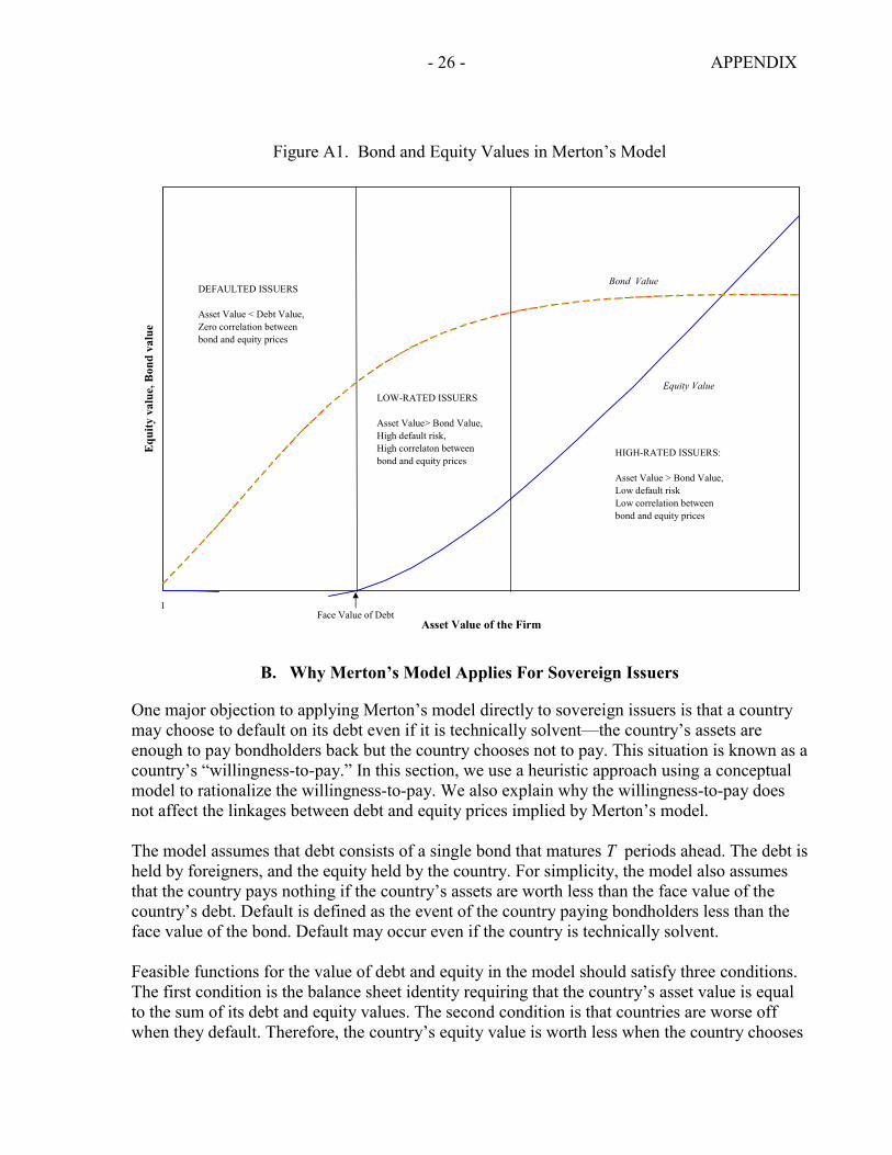
In the model, bond and equity prices are always positively correlated. The degree of correlation, however, depends directly on the firm’s leverage. In the extreme case that B/E ≈ 0, the correlation is also negligible. This discussion is summarized graphically in the figure below.

- 26 - APPENDIX

Figure A1. Bond and Equity Values in Merton’s Model

Equity Value

Bond Value

1

Asset Value of the Firm

Equ

ity v

alue

, Bon

d va

lue

Face Value of Debt

DEFAULTED ISSUERS

Asset Value < Debt Value,Zero correlation between bond and equity prices

LOW-RATED ISSUERS

Asset Value> Bond Value,High default risk,High correlaton betweenbond and equity prices

HIGH-RATED ISSUERS:

Asset Value > Bond Value,Low default riskLow correlation between bond and equity prices

B. Why Merton’s Model Applies For Sovereign Issuers

One major objection to applying Merton’s model directly to sovereign issuers is that a country may choose to default on its debt even if it is technically solvent—the country’s assets are enough to pay bondholders back but the country chooses not to pay. This situation is known as a country’s “willingness-to-pay.” In this section, we use a heuristic approach using a conceptual model to rationalize the willingness-to-pay. We also explain why the willingness-to-pay does not affect the linkages between debt and equity prices implied by Merton’s model. The model assumes that debt consists of a single bond that matures T periods ahead. The debt is held by foreigners, and the equity held by the country. For simplicity, the model also assumes that the country pays nothing if the country’s assets are worth less than the face value of the country’s debt. Default is defined as the event of the country paying bondholders less than the face value of the bond. Default may occur even if the country is technically solvent. Feasible functions for the value of debt and equity in the model should satisfy three conditions. The first condition is the balance sheet identity requiring that the country’s asset value is equal to the sum of its debt and equity values. The second condition is that countries are worse off when they default. Therefore, the country’s equity value is worth less when the country chooses

- 27 - APPENDIX

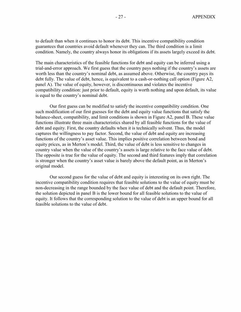
to default than when it continues to honor its debt. This incentive compatibility condition guarantees that countries avoid default whenever they can. The third condition is a limit condition. Namely, the country always honor its obligations if its assets largely exceed its debt. The main characteristics of the feasible functions for debt and equity can be inferred using a trial-and-error approach. We first guess that the country pays nothing if the country’s assets are worth less than the country’s nominal debt, as assumed above. Otherwise, the country pays its debt fully. The value of debt, hence, is equivalent to a cash-or-nothing call option (Figure A2, panel A). The value of equity, however, is discontinuous and violates the incentive compatibility condition: just prior to default, equity is worth nothing and upon default, its value is equal to the country’s nominal debt.

Our first guess can be modified to satisfy the incentive compatibility condition. One such modification of our first guesses for the debt and equity value functions that satisfy the balance-sheet, compatibility, and limit conditions is shown in Figure A2, panel B. These value functions illustrate three main characteristics shared by all feasible functions for the value of debt and equity. First, the country defaults when it is technically solvent. Thus, the model captures the willingness to pay factor. Second, the value of debt and equity are increasing functions of the country’s asset value. This implies positive correlation between bond and equity prices, as in Merton’s model. Third, the value of debt is less sensitive to changes in country value when the value of the country’s assets is large relative to the face value of debt. The opposite is true for the value of equity. The second and third features imply that correlation is stronger when the country’s asset value is barely above the default point, as in Merton’s original model.

Our second guess for the value of debt and equity is interesting on its own right. The incentive compatibility condition requires that feasible solutions to the value of equity must be non-decreasing in the range bounded by the face value of debt and the default point. Therefore, the solution depicted in panel B is the lower bound for all feasible solutions to the value of equity. It follows that the corresponding solution to the value of debt is an upper bound for all feasible solutions to the value of debt.

- 28 - APPENDIX

Figure A2. Sovereign Issuers: Value of Debt and Equity

Country Value

Deb

t and

Equ

ity V

alue

s

Value of Equity

Value of Debt

Face Value of Debt

Panel A

Country Value

Deb

t and

Equ

ity V

alue

s

Default Point

Value of Equity

Value of Debt

Face Value of Debt

Panel B

- 29 -

References Azarchs, Tanya, 2003, “Demystifying Banks’ Use of Credit Derivatives,” Standard and Poors,

December 9. Blanco, Roberto, Simon Brennan, and Ian W. Marsh, 2003, “An Empirical Analysis of the

Dynamic Relationships Between Investment Grade Bonds and Credit Default Swaps” (unpublished; Madrid: Banco de España, and London: Bank of England).

Baillie, Richard T., G. Geoffrey Booth, Yiuman Tse, and Tatyana Zabotina, 2002, “Price

Discovery and Common Factor Models,” Journal of Financial Markets, Vol. 5, pp. 309–21.

Booth, G. Geoffrey, Teppo Martikainen, and Yiuman Tse, 1997, “Price and Volatility

Spillovers in Scandinavian Stock Markets,” Journal of Banking and Finance, Vol. 21, pp. 811–23.

Chan-Lau, Jorge A., 2003, “Anticipating Credit Events Using Credit Default Swaps, with an

Application to Sovereign Debt Crises,” IMF Working Paper 03/106 (Washington: International Monetary Fund).

Duffie, Darrell J., 1999, “Credit Swap Valuation,” Financial Analysts Journal, Vol. 55, pp.

73–87. FitchRatings, 2003, Global Credit Derivatives: A Qualified Success, September. Gonzalo, Jesús, and Clive W.J. Granger, 1995, “Estimation of Common Long-Memory

Components in Cointegrated Systems,” Journal of Business and Economic Statistics, Vol. 13, pp. 27–35.

Granger, Clive W.J., 1969, “Investigating Causal Relations by Econometric Models and Cross-

Spectral Methods,” Econometrica, Vol. 37, pp. 424–38. _____, and P. Newbold, 1974, “Spurious Regressions in Econometrics,” Journal of

Econometrics, Vol. 2, pp. 111–120. Hamao, Yasushi, Ronald W. Masulis, and Victor Ng, 1990, “Correlations in Price Changes and

Volatility Across International Stock Markets,” Review of Financial Studies, Vol. 3, pp. 281–307.

Hasbrouck, Joel, 1995, “One Security, Many Markets: Determining the Contributions to Price

Discovery,” Journal of Finance, Vol. 50, pp. 1175–99. Hayashi, Fumio, 2000, Econometrics (Princeton: Princeton University Press)

- 30 -

Hull, John C., Mirela Predescu, and Alan White, 2003, “The Relationship Between Credit

Default Swap Spreads, Bond Yields, and Credit Rating Announcements” (unpublished; Toronto: University of Toronto).

Hull, John C., and Alan White, 2000, “Valuing Credit Default Swaps I: No Counterparty

Default Risk,” Journal of Derivatives, Vol. 8, pp. 29–40. International Monetary Fund, 2003, Global Financial Stability Report, September

(Washington). Johansen, Soren, 1991, “Estimation and Hypothesis Testing of Cointegration Vectors in

Gaussian Vector Autoregressive Models,” Econometrica, Vol. 59, pp. 1551–80. Lehmann, Bruce N., 2002, “Some Desiderata for the Measurement of Price Discovery Across

Markets,” Journal of Financial Markets, Vol. 5, pp. 259–76. Longstaff, Francis, Sanjay Mithal, and Eric Neiss, 2003, “The Credit Default Swap Market: Is

Credit Protection Priced Correctly” (unpublished; Los Angeles: University of California).

Merton, Robert C., 1974, “On the Pricing of Corporate Debt: The Risk Structure of Interest

Rates,” Journal of Finance, Vol. 29, pp. 449–70. Stock, James H., and Mark W. Watson, 1988, “Testing for Common Trends,” Journal of the

American Statistical Association, Vol. 83, pp. 1097–07. Tavakoli, Janet, 1998, Credit Derivatives (New York: John Wiley and Sons). Xu, David, 2003, Emerging Markets Credit Derivatives (New York: Deutsche Bank).