U.U.D.M. Project Report 2011:24

Examensarbete i matematik, 15 hpHandledare och examinator: Johan TyskDecember 2011

Department of MathematicsUppsala University

Pricing Callable Bonds

Jiang Xue

1

ACKNOWLEDGEMENTS

This thesis has received a lot of assistance and support frommany sides. My sincere

acknowledgement goes to my thesis supervisor Professor Johan Tysk. He inspired me

to work on this thesis and has been supporting me for almost2 years. His patience,

inspiration, kindness and guidance have kept me continuously focusing on this work to

today.

I am also indebted to Kailing Zeng and Jun Han whose help is of great importance

to my work. Meanwhile, I will extend my thanks to all the teachers in the financial

mathematics programme who gave us the fundamental knowledge in this area.

Finally, I would also like to offer my gratitude to my family.Their constant support

is indispensable for my research and study.

CONTENTS

I Introduction iv

II Interest Rate Models vi

II-A Single-factor models . . . . . . . . . . . . . . . . . . . . . . . . . vi

II-A1 The Merton model (1973) . . . . . . . . . . . . . . . . vii

II-A2 The Vasicek model (1977) . . . . . . . . . . . . . . . vii

II-A3 The Brennan and Schwartz model (1980) . . . . . . . vii

II-A4 The Marsh Rosenfeld model (1983) . . . . . . . . . . viii

II-A5 The Cox, Ingersoll and Ross (CIR) model (1985) . . . viii

II-A6 The Hull-White model (1993) . . . . . . . . . . . . . ix

II-A7 The Lognormal model (1987) . . . . . . . . . . . . . . ix

III Options x

III-A Value the option . . . . . . . . . . . . . . . . . . . . . . . . . . . x

III-A1 Black-Scholes equation . . . . . . . . . . . . . . . . . x

III-A2 European options . . . . . . . . . . . . . . . . . . . . xii

IV Finite Difference Methods xiii

IV-A Basic knowledge of numerical differentiation . . . . . . . .. . . xiv

IV-B Types of finite difference methods . . . . . . . . . . . . . . . . . xvi

V Pricing Callable Bonds xvii

V-A Pricing zero-coupon bonds with the CIR model . . . . . . . . . . xvii

V-A1 Pricing zero-coupon bonds . . . . . . . . . . . . . . . xvii

V-A2 Pricing bonds with European call options . . . . . . . xx

V-B Pricing zero-coupon bonds with Vasicek model . . . . . . . . .. xxiii

V-B1 Vasicek model . . . . . . . . . . . . . . . . . . . . . . xxiii

V-B2 Pricing bonds with European call options . . . . . . . xxvi

ii

VI Conclusion xxix

Appendix A: Matlab programme for pricing the zero-coupon bond without

option (Fig. 1) xxx

Appendix B: Matlab programme for pricing the zero-coupon bond based on

the Vasicek model (Fig. 5) xxxi

References xxxiv

iii

Abstract

In this paper, we value callable bonds. The interest rate process considered follows the

Vasicek or the Cox-Ingersoll-Ross (CIR) models. Our analytical results are reached using the

implicit Euler finite difference method. This paper is organized as follows: Section I introduces

different interest rate models for fixed income securities.We study the European options in

Section II. The finite difference method for solving the partial differentiation equations (PDE)

is shown in Section III. The finite difference method appliedfor pricing callable bonds is

investigated in Section IV. Finally, Section V concludes the paper. All the programming is

done in MATLAB, and the corresponding code can be found in theAppendix.

Index Terms

Callable bonds, finite difference, Vasicek, CIR, European option.

iv

I. I NTRODUCTION

Financial innovation has developed rapidly during recent years. The traditional fi-

nancial products offered by the corporations and governments to raise funds, such as

equity, debt, preferred stock and convertibles, gave way tothe new innovations which

include options, bonds with embedded options, securitizedassets, etc.

A callable bond is a type of bond which allows the issuing entity to retire the bond

with a strike price at some date before the bond reaches the date of maturity [1]. We

can view the callable bond as a combination of a non-option bond and a call option

which is based on that bond. The writer of the call option is the holder of the bond,

and the holder of the call option is the bond issuing corporation. Thus the price of a

callable bond is the value of the straight bond less the valueof the call option [2]. The

value of the call option must converge to zero if the bond price is lower than the strike

price or the bond close to maturity.

We should note that the call option of the callable bond is nota separable option in

the sense that it could be traded in the open market. In other words, the bond and call

option are always traded together. The issuer pays a higher coupon rate for the callable

bond because of the call option. The bond will be retired at the call date if the interest

rate in the market has gone down, which means the price of the bond has gone up.

In this situation, the issuer will be able to refinance its debt (bond) at a cheaper level

and it will be incentivized to call the bonds it originally issued. So, the value of the

callable bond relates tightly to the interest rate. The callable bond is a choice for the

issuers who want to avoid the risk of interest rate decreasing (bond price increasing).

Each time an issuer use his right to call such a bond, the issuer is able to issue another

callable bond with lower coupon (or higher price of zero-coupon bond). However, by

comparing two zero-coupon bonds identical in all respects except that one of them is a

callable bond, we may infer that the price of the callable bond must be lower than the

price of the non-option zero-coupon bond to induce the investors to buy the callable

v

bond. In effect, the strategy of repeatedly calling and reissuing new callable bonds is

like “marking to market” changes in interest rate [2].

In our paper, we will analyze the problem of pricing the zero-coupon bond based on

the Vasicek and CIR interest rate models by the finite difference method.

vi

II. I NTERESTRATE MODELS

Zero-coupon bonds are the kinds of discount bonds which are sold at a price below

the face value at timet and pay the face value at the time of maturityT . We define

the value of the zero-coupon bond asB(t, T ). Then, we know thatB(t, T ) is the value

of the bond at timet andB(T, T ) = 1. By this definition, the bond value will keep

increasing to1 from time t to t = T . When interest rate is constant, we can express

the simplest model as

B(t, T )e(T−t)R(t,T ) = 1 (1)

whereR(t.T ) is the yield to maturity of the zero-coupon bondB(t, T ).

First, we introduce the following basic definitions to the readers:

• Instantaneous risk-free interest rate (short-term interest rate)r(t):

r(t) = limT→t

R(t, T ). (2)

• Forward ratef(t, T1, T2):

f(t, T1, T2) =lnB(t, T1)− lnB(t, T2)

T1 − T2

, (3)

it means the interest rate which is agreed at timet for the risk-free loan beginning

at timeT1 and ending at timeT2.

• Instantaneous forward ratef(t, T ):

f(t, T ) = f(t, T, T ), (4)

it is the limitation of forward ratef(t, T1, T2).

A. Single-factor models

In single-factor model of interest rate, we assume that all security prices and rates

depend on only one factor – the short-term interest rate. In our model, the short-term

vii

interest rate can be given by the stochastic differential equation (SDE) as,

dr(t) = µr()dt+ σr()dW (t) (5)

whereµr ≡ µr(t, r(t)), σr ≡ σr(t, r(t)) are defined as real-value functions andW (t), t ≥

0 is the random Wiener process.

There are a lot of single-factor models for the short-term interest rate. Generally

speaking, the different short-term interest rate SDE depends on the different kinds of

functionsµr andσr. Most of the SDE models are named after the people who invented

them.

1) The Merton model (1973):It is one of the first works to propose a stochastic

model for the short-term interest rate,

dr(t) = µrdt+ σrdW (t) (6)

whereµr andσr are constant and the risk market premiumλ is assumed to be constant.

2) The Vasicek model (1977):Vasicek use a mean-reverting Ornstein-Uhlenbeck

process to model the short-term interest rate,

dr(t) = K(θ − r(t))dt+ σdW (t) (7)

whereK, θ andσ are positive constants and he assume the risk market premiumλ is

constant.

This model fit well for the zero-coupon bonds and several European-style interest rate

derivatives. However, with very low probability, this model has the undesirable property

of allowing negative interest rate.

3) The Brennan and Schwartz model (1980):Brennan and Schwartz were forerunner

on the area of pricing the options embedded bonds. The model of the short-term interest

viii

rate which they are given as,

dr(t) = K(θ − r(t))dt+ σr(t)dW (t) (8)

whereK, θ andσ are positive constants and the risk market premiumλ is assume to

be constant.

In this model, the interest rate move as a geometric Brownian motion which is a

mean-reverting proportional process to price the conversion options.

4) The Marsh Rosenfeld model (1983):The Marsh-Rosenfeld model corresponds to

the constant-elasticity-of-variance process and is expressed as,

dr(t) = −Kr(t)dt+ σr(t)αdW (t) (9)

whereK, α andσ are positive constants and the model assumes the risk marketpremium

λ is constant.

This model is considered as an alternative process for the short-term interest rate

among others.

5) The Cox, Ingersoll and Ross (CIR) model (1985):The CIR model used the mean-

reverting square-root process to describe the movements ofshort-term interest rate. It

is given by,

dr(t) = K(θ − r(t))dt+ σ√

r(t)dW (t) (10)

whereK, θ and σ are positive constants. The market risk premium at equilibrium is

expressed as,

λ(r, t) = λ√

r(t). (11)

The CIR model is extensible to several factors and make sure the interest rates to

be strictly positive. Based on this model, we can derive the closed-form solutions for

zero-coupon bonds and some European-style interest rate derivatives.

ix

All of the above models can not be calibrated with yield curves. Therefore, some

new models were introduced to overcome these problems and are consistent with the

above models.

6) The Hull-White model (1993):The Hull-White model leads to the generalized

Vasicek and CIR models and is given by,

dr(t) = ((θ(t)−K(t))r(t))dt+ σ(t)rβ(t)dW (t) (12)

where all the coefficients in the model are functions of time and can be used to calibrate

exactly the model to current market prices. The market risk premium is expressed as,

λ(r, t) = λrν , with λ ≥ 0 andν ≥ 0. (13)

The disadvantage of this model is that we can not derive the analytical result of the

bond option price. However, we can derive the numerical result by the other methods,

such as finite difference method.

7) The Lognormal model (1987):The Lognormal model is different from all the other

models which we mentioned before. The previous models abovemodel the interest rate

as Gaussian process. Using Gaussian process, the interest rates can be negative with a

positive probability and this implies arbitrage opportunities. However, the Lognormal

model does not have this problem and can be expressed as,

d log(r(t)) = (θ(t)−K log(r(t)))dt+ σrdW (t) (14)

This incorporates the mean reversion feature of the interest rate.

In our paper, we are pricing the zero-coupon callable bond based on the Vasicek and

CIR short-term interest rate models.

x

III. O PTIONS

Options are the kinds of derivative financial instrument. They are sold by the option

writer to the option holder by contract. In the contracts (Options), the buyer (holder) has

the right, but not the obligation, to buy (call) or sell (put)a security or other financial

asset at an agreed price (the strike price) during a certain period of time (American

options) or on a specific (exercise) date (European options). Options can be used in

many different ways as extremely versatile securities. They can be used to avoid the

currency exchange risk and trading risk. Traders use options to speculate, which is a

relatively risky practice, while hedgers use options to reduce the risk of holding an

asset.

A. Value the option

We denote the value of the option byV (S, t). It means the valueV is a function of

the current value of the underlying asset,S, and time parameter,t. At time t1, we know

that Vt1 = V (St1 , t1). σ is the volatility of the underlying asset. The exercise price of

the option is noted byX. T is the expiry time and also the interest rate isr as we

mentioned before.

1) Black-Scholes equation:We will introduce the Black-Scholes equation (model)

before we price the options. Black and Scholes started the serious study of the theory of

option pricing. All further advances in this field have been extensions and refinements

of the original idea expressed in [3]. In our work, we follow the assumptions which

involved in the derivation of the Black-Scholes equation.

• We know the risk-free interest rater(t) and the volatility of assetσ are functions

of time t over the life of the options and zero-coupon bonds.

• The market falls into the efficient market hypothesis. It means that the market

is liquid, has price-continuity, is fair, no arbitrage opportunities and provides all

players with equal access to available information. It implies that the Black-Scholes

xi

model assume no transaction cost, underlying security is perfectly divisible and the

short selling with full use of proceeds is possible.

• The asset price follows the lognormal random process.

• No dividend is paid during the life of the options.

Based on [4], we assume that there is a general derivativeV whose value is a function

of the value of the underlying securityS(t). S(t) follows the stochastic process,

dS(t) = αS(t)dt+ σS(t)dW (t), (15)

where the constant coefficientα is the average growth rate of the underlying security

andσ is the volatility.

We suppose that the derivative can be traded on an ideal market and its process has

the formV (t, S(t)). We obtain the following theorem.

Theorem 1:From the no-arbitrage condition, the pricing function ofV (t, S(t)) is the

function whenV (t, S(t)) is the solution of the following boundary PDE problem in the

domain[0, T ]× rmax,

∂V (t, S(t))

∂t+ rS(t)

∂V (t, S(t))

∂S(t)+

1

2S(t)2σ2(t, S(t))

∂2V (t, S(t))

∂S(t)2− rV (t, S(t)) = 0

(16)

with the boundary att = T ,

V (T, S(T )) = Φ(S(T )) (17)

whereΦ(S(t)) is a simple claim ofS(t) at time t.

The functionV (t, S(t)) will be the price of the European option if we consider

Φ(S(T )) to be the payoff function at timeT . Meanwhile, we have to confirm the

boundary and final conditions in order to have a unique solution when we solve the

above PDE problem.

xii

2) European options:The European options are the options that can only be exercised

at expiration. The value of the options at expiration date are,

V (ST , T ) =

(ST −X)+ call options

(X − ST )+ put options

(18)

where(a− b)+ = max(0, a− b).

Specially, we just think about the pricing problem of European call option in our

paper. The value of the call options are denoted byC(t, S) with the expiry dateT

and strike priceX. We derive that the value of the call option at timet = T can be

expressed as the payoff function,

C(t, S) = max(S −X, 0) (19)

This is the final condition of option pricing problem at timeT . Meanwhile, we also

need to find out the boundary conditions for our problem. For general call options, the

boundary conditions can be find out atS = 0 andS −→ ∞. However, the maximum

price of the zero-coupon bonds is their face value. It means the boundary conditions of

the European call options based on the zero-coupon bonds areapplied atS = 0 and

S = BT . In [5], we know the price of call options will remain zero, ifS is ever zero.

So, we get the boundary conditions as,

C(t, 0) = 0, when S = 0, (20)

C(t, S) = BT −X, when S = BT . (21)

With the conditions above, we can derive the Black-Scholes’ value of the European

call options.

xiii

IV. F INITE DIFFERENCEMETHODS

The goal of our paper is to develop an accurate and efficient numerical method to

price the zero-coupon callable bonds in quantitative finance based on our knowledge

of finance and PDE. However, it is very difficult or even impossible to find the exact

closed-form solutions for the PDE problems. Also, it may be very difficult to calculate

even if we can find the closed-form solutions. For these reasons, we have to involve

the approximate methods. There are several commonly used approximate methods as

followings which mentioned in [6],

• Lattice method. It includes the binomial and trinomial models, assuming that the

underlying stochastic process is discrete i.e. the underlying asset ”jumps” to a

finite number of values (each associated with a certain probability) with a small

advancement in time.

• Monte Carlo method. It is a class of computational algorithmsthat rely on repeated

random sampling to compute their results. It is based on the law of great number.

Monte Carlo methods are often used in simulating physical andmathematical

systems. These methods are most suited to calculate by a computer and tend to be

used when it is infeasible to compute an exact result with a deterministic algorithm.

This method is also used to complement the theoretical derivations.

• Finite Difference method. In mathematics, finite-difference methods are numeri-

cal methods for approximating the solutions to differential equations using finite

difference equations to approximate derivatives. They consist of discretizing the

PDEs and the given boundary conditions to form a set of difference equations and

can be solved either directly or iteratively. These methodshave a long history and

have been applied for more than 200 years to approximate the solutions of PDEs

in physical sciences and engineering.

In our paper, we use the finite difference methods to solve thePDEs of pricing the

zero-coupon callable bonds.

xiv

A. Basic knowledge of numerical differentiation

Supposing, we have a real-valued function of a real variable, such as [7],

y = f(x). (22)

The things which we are most interested are how to find the approximations to the

first and second derivatives of the functionf(x). In general, we do not know the form

of the functionf(x). So, we can not calculate the derivatives off(x) analytically. In

this situation, we involve the methods to numerical approximations. For example, we

want to approximate the first derivative off(x) at point a and h is a small (usually)

positive constant number. The first derivative of functionf(x) at pointa can be given

by,

• Centred difference formula:f ′(a) = f(a+h)−f(a−h)2h

;

• Forward difference formula:f ′(a) = f(a+h)−f(a)h

;

• Backward difference formula:f ′(a) = f(a)−f(a−h)h

;

In our paper, we use the following notations for short,

D0f(a) =f(a+ h)− f(a− h)

2h, (23)

D+f(a) =f(a+ h)− f(a)

h, (24)

D−f(a) =f(a)− f(a− h)

h, (25)

Lemma 1:The centred difference formula gives a second order approximation to the

first derivative ifh is small enough and iff(x) has continuous derivatives up to3.

xv

Proof: We use the Taylor’s expansion to expandf(x) at pointa as,

f(a± h) = f(a)± hf ′(a) +h2

2!f ′′(a) +

h3

3!f ′′(η±) (26)

where

η− ∈ (a− h, a), andη+ ∈ (a, a+ h). (27)

Substituting equation (26) into equation (23), we derive,

D0f(a) = f ′(a) +h2

3!

(

f ′′′(η+) + f ′′′(η−)

2

)

. (28)

From the equation above, we proofed lemma 1.

In the same way, we can say that the forward and backward difference formulas give

first order approximation to the first derivative off(x) at pointa, as,

D+f(a) = f ′(a) +h

2f ′′(η+), η+ ∈ (a, a+ h) (29)

and

D−f(a) = f ′(a)−h

2f ′′(η−), η− ∈ (a− h, a). (30)

The one side schemes place low continuity constraints on thefunction f(x) because

they are first order accurate. We just need to assume that its second order derivative is

continuous.

For the second derivative off(x) at pointa, we use the following three points formula

[8],

D+D−f(a) ≡f(a− h)− 2f(a) + f(a+ h)

h2. (31)

It is a second order approximation to the second order derivative of f(x) at pointa

and we assume that the functionf(x) has continuous derivatives up to and including

xvi

order4. The error of discretisation is given by,

D+D−f(a) = f ′′(a) +h4

4!(f (iv)(η+) + f (iv)(η−)). (32)

B. Types of finite difference methods

We need to consider the properties of consistency, stability and convergence of the

scheme when we are using the finite difference methods. The details of the proof of

these properties can be found in [7] and [9]. The main finite difference methods are as

following,

• Explicit finite difference method. In this method, we use theforward difference

formula.

• Implicit finite difference method. In this method, we use thebackward difference

formula.

• Crank-Nicholson finite difference method. In this method, weuse the centred

difference formula.

In our paper, we use the implicit Euler scheme to solve our PDEs problem of pricing

the callable bond.

xvii

V. PRICING CALLABLE BONDS

The callable bonds are the zero-coupon bonds embedded call option (European).

Generally, we can say that,

Price of callable bond =Price of option free zero− coupon bond

− Price of embedded option. (33)

Next, we will price the option-free zero-coupon bonds and callable bonds separately.

A. Pricing zero-coupon bonds with the CIR model

We use the implicit method to solve this PDEs problem. We discretize the interest

rater into N equally spaced units ofδr, and the time variablet into M equally spaced

units of δt,

rj = jδr, j = 0, · · · , N ; (34)

ti = iδt, i = 0, · · · ,M. (35)

1) Pricing zero-coupon bonds:In this part, we price the zero-coupon bonds based

on the CIR model.

When j = N , rj = rmax. Please note that we are using the engineering’s time. It

means thatti = T when i = 0.

Letting a = Kθ and K = b, the pricing problem of zero-coupon bond can be

expressed as,

−∂B(r(t), t)

∂t+

1

2r(t)σ2∂

2B(r(t), t)

∂r(t)2+ (a− br(t))

∂B(r(t), t)

∂r(t)− r(t)B(r(t), t) = 0,

(36)

The boundary conditions were investigated thoroughly in [11] and can be expressed

xviii

as,

B(rmax, t) = 0, t > 0; (37)

−∂B(0, t)

∂t+ a

∂B(0, t)

∂r= 0, t > 0 anda > 0; (38)

B(r, 0) = 1 (facevalue), 0 < r < rmax. (39)

Notice, we do not know the bond value atr = 0 and use the implicit Euler scheme

for the Black-Scholes equation as,

−Bi+1

j −Bij

δt+

1

2σ2ri+1

j D+D−Bi+1j + (a− bri+1

j )D0Bi+1j − rjB

i+1j = 0, 1 ≤ j ≤ N − 1;

(40)

whereBij = B(rj, ti).

This equation can be rewritten as,

−Bi+1

j −Bij

δt+

1

2σ2ri+1

j

Bi+1j−1 − 2Bi+1

j +Bi+1j+1

(δr)2+ (a− bri+1

j )Bi+1

j+1 − Bi+1j−1

2δr− rjB

i+1j = 0,

1 ≤ j ≤ N − 1.

(41)

Easily, we have,

Bij = ajB

i+1j−1 + bjB

i+1j + cjB

i+1j+1, with j = 1, · · · , N − 1 and i = 1, · · · ,M, (42)

where

aj =1

2aδt

δr− bδt

1

2(j − 1)− σ2 δt

δr(j − 1); (43)

bj = 1 + δr(j − 1)δt+ σ2 δt

δr(j − 1); (44)

cj = bδt1

2(j − 1)− aδt

1

2δr− σ2δt

1

2δr(j − 1). (45)

For boundary conditions, we have,

xix

0 0.5 1 1.5 2 2.5 3 3.50

0.1

0.2

0.3

0.4

0.5

0.6

0.7

0.8

0.9

1

Interest Rate r

Ze

ro−

cou

po

n B

on

d P

rice

B(r

, t)

5 years7 years10 years20 years

Fig. 1: Price of5, 7, 10 and20 years zero-coupon bonds with expiration for differentinterest rate, based on the CIR model.

•

−Bi+1

j − Bij

δt+ a

Bi+1j+1 −Bi+1

j

δr= 0, when j = 0 (r = 0). (46)

•

BiN = 0, when j = N (r = rmax). (47)

•

B0j = face value, when t = 0 (at expiration date). (48)

Fig. 1 depicts the value of5 years zero-coupon bond with face value1. We suppose

that the parameters in CIR model asa = bδ, b = 0.54958 and δ = 0.38757. It shows

the interest rate changes from0 to 350% and the bond price decrease from face value

xx

to 0. It fit our knowledge well that the bond price decrease when the time of maturity

increase.

2) Pricing bonds with European call options:The bonds with European call options

just have a single possible call date. We denote the call dateby τc and define the

engineering timetc = T − τc. Meanwhile, we denote the notice time asτn and the

engineering time astn = T − τn. Also, we denote the call price isX. In general, we

assume that it is optimal for the issuer to minimize the valueof the contract. It means

the issuer will exercise the options if the price of the callable bonds exceed the exercise

price at the notice date. Otherwise, the issuer will give up the right of the call options

and the callable bonds price are equal to the price of non-option bonds.

We call the interest raterb is the “break-even” interest rate if the issuer is indifferent

between exercising the options or not doing so with the interest raterb at the notice

dateτn. In [10], we can find the “break-even” interest rate by,

XB(rb, tn − tc)− P (rb, t−

n ) = 0, (49)

whereB(rb, tn− tc) is the value at timetn of the zero-coupon bond maturing attc with

face value and satisfies the equation (36),t+n (t−n ) means the time immediately after

(before) the notice date andP (rb, t−

n ) denote the price of the callable bonds an instant

before the notice date.

For finding the “break-even” interest rate, i.e. solving theequation (49), we know

the value of callable bondsP (rb, t−

n ) at the time before the notice date are equal to the

value of non-option bonds. The solution of equation (49) is the cross point between the

curve of non-option bondsP (rb, t−

n ) and the curve of zero-coupon bondsB(rb, tn − tc)

product the exercise priceX.

Fig. 2 shows the “break-even” interest rate for callable bonds with strike price0.8

and notice date at 5 years before maturity. We suppose the time between the call date

and the notice date,tn − tc, is 0.1 years. The “break-even” interest rate isrb = 0.11.

xxi

0 0.2 0.4 0.6 0.8 1 1.2 1.4 1.60

0.1

0.2

0.3

0.4

0.5

0.6

0.7

0.8

0.9

1

Interest Rate r

Bo

nd

Price

B(r

, t)

P(rb, t

n−)

X B(rb, t

n−t

c)

rb=0.11

Fig. 2: The “break-even” interest rate for callable bonds with exercise price0.8 at thenotice date which is5 years before maturity, based on the CIR model.

For pricing the callable bonds, we should update the callable bonds price after we find

the “break-even” interest rate. We price the callable bondsat the notice date because

the interest rate at notice date determine the price of the zero-coupon callable bonds.

At this situation, we can price the zero-coupon callable bonds at the notice date as [12],

P (rb, t+n ) =

XB(r, tn − tc) if r ≤ rb

P (rb, t−

n ) if r ≥ rb

. (50)

The process for pricing the zero-coupon callable bonds is,

• Step1, finding the “break-even” interest rate,rb, by solving the equation (49);

• Step2, pricing the callable bonds at notice date as equation (50) for different range

of r.

Fig. 3 plots the value of zero-coupon callable bonds at notice date3 years before

xxii

0 0.5 1 1.50.1

0.2

0.3

0.4

0.5

0.6

0.7

0.8

0.9

1

Interest Rate r

Bo

nd

Price

non−option bond

callalbe bond

rb=0.161

Fig. 3: The value of zero-coupon callable bonds with exercise price0.8 at the noticedate which is3 years before maturity, based on the CIR model.

the maturity. We suppose the strike price of the embeded calloptions is0.8, the time

between the call date and the notice date istn − tc = 0.1 year and the face value of

the callable bond is1. We can see that the “break-even” interest rate isrb = 0.161.

Meanwhile, the parameters of CIR model are set as mentioned before.

Fig. 4 illustrates the value of zero-coupon callable bonds at notice date2 years before

the maturity. We derive that the “break-even” interest rateis rb = 0.161. The call price is

0.7 and the time between the call date and the notice date is2 month, i.e.tn−tc = 0.167.

The bond will pay1 at the maturity and the others parameters as mentioned before.

xxiii

0 0.2 0.4 0.6 0.8 1 1.2 1.4 1.60.1

0.2

0.3

0.4

0.5

0.6

0.7

0.8

0.9

1

Interest Rate r

Bo

nd

Price

callable bond

non−option bond

"break even" interest rate, rb=0.35

Fig. 4: The value of zero-coupon callable bonds with exercise price0.7 at the noticedate which is2 years before maturity, based on the CIR model.

B. Pricing zero-coupon bonds with Vasicek model

1) Vasicek model:Based on the Vasicek interest rate model and the assumption we

mentioned before, the pricing problem of zero-coupon bond can be expressed as,

−∂B(r(t), t)

∂t+

1

2σ2∂

2B(r(t), t)

∂r(t)2+ (a− br(t))

∂B(r(t), t)

∂r(t)− r(t)B(r(t), t) = 0, (51)

where a = Kθ and b = K. One of the disadvantages of the Vasicek model is that

the interest rate may be negative in this model. Based on the practical experience, we

know that the equation (51) holds the following boundary conditions whenr(t) is not

negative.

xxiv

Whenr(t) = 0, (51) can be transform to,

−∂B(0, t)

∂t+

1

2σ2∂

2B(r(t), t)

∂r(t)2+ a

∂B(0, t)

∂r= 0, t > 0; (52)

Whenr(t) = rmax and t = 0, we get,

B(rmax, t) = 0, t > 0; (53)

B(r, 0) = 1 (facevalue), 0 < r < rmax. (54)

Using the implicit Euler scheme for the Black-Scholes equation, we derive that,

−Bi+1

j −Bij

δt+

1

2σ2D+D−B

i+1j + (a− bri+1

j )D0Bi+1j − rjB

i+1j = 0, 1 ≤ j ≤ N − 1;

(55)

whereBij = B(rj, ti).

We can rewrite the equation (55) as,

−Bi+1

j −Bij

δt+

1

2σ2

Bi+1j−1 − 2Bi+1

j + Bi+1j+1

(δr)2+ (a− bri+1

j )Bi+1

j+1 −Bi+1j−1

2δr− rjB

i+1j = 0,

1 ≤ j ≤ N − 1.

(56)

Then, we have,

Bij = a

′

jBi+1j−1 + b

′

jBi+1j + c

′

jBi+1j+1, with j = 1, · · · , N − 1 and i = 1, · · · ,M, (57)

where

a′

j =1

2aδt

δr−

1

2bδt(j − 1)−

1

2σ2 δt

(δr)2; (58)

b′

j = 1 + δr(j − 1)δt+ σ2 δt

(δr)2; (59)

c′

j =1

2bδt(j − 1)− aδt

1

2δr− σ2δt

1

2(δr)2. (60)

For boundary conditions, we have,

xxv

0.1 0.2 0.3 0.4 0.5 0.6 0.7 0.8 0.9 10

0.1

0.2

0.3

0.4

0.5

0.6

0.7

0.8

0.9

1

Interest Rate r

Ze

ro−

co

up

on

Bo

nd

Price

B(r

, t)

5 years7 years10 years20 years

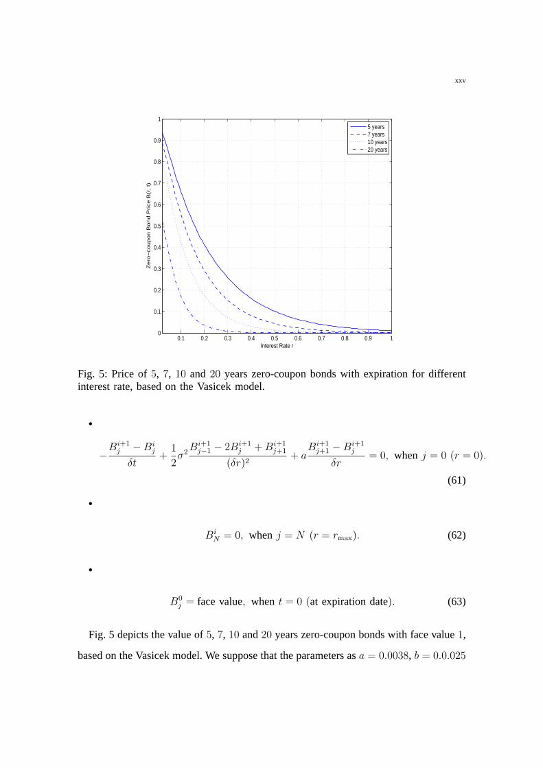
Fig. 5: Price of5, 7, 10 and20 years zero-coupon bonds with expiration for differentinterest rate, based on the Vasicek model.

•

−Bi+1

j −Bij

δt+

1

2σ2

Bi+1j−1 − 2Bi+1

j + Bi+1j+1

(δr)2+ a

Bi+1j+1 − Bi+1

j

δr= 0, when j = 0 (r = 0).

(61)

•

BiN = 0, when j = N (r = rmax). (62)

•

B0j = face value, when t = 0 (at expiration date). (63)

Fig. 5 depicts the value of5, 7, 10 and20 years zero-coupon bonds with face value1,

based on the Vasicek model. We suppose that the parameters asa = 0.0038, b = 0.0.025

xxvi

0 0.2 0.4 0.6 0.8 1 1.20

0.1

0.2

0.3

0.4

0.5

0.6

0.7

0.8

0.9

1

Interest Rate r

Bon

d P

rice

callable bond

rb=0.09

non−option bond

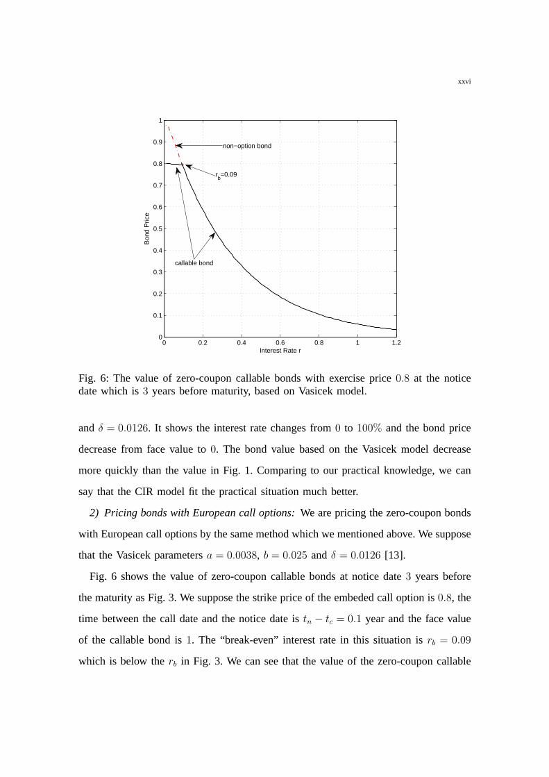
Fig. 6: The value of zero-coupon callable bonds with exercise price0.8 at the noticedate which is3 years before maturity, based on Vasicek model.

andδ = 0.0126. It shows the interest rate changes from0 to 100% and the bond price

decrease from face value to0. The bond value based on the Vasicek model decrease

more quickly than the value in Fig. 1. Comparing to our practical knowledge, we can

say that the CIR model fit the practical situation much better.

2) Pricing bonds with European call options:We are pricing the zero-coupon bonds

with European call options by the same method which we mentioned above. We suppose

that the Vasicek parametersa = 0.0038, b = 0.025 andδ = 0.0126 [13].

Fig. 6 shows the value of zero-coupon callable bonds at notice date3 years before

the maturity as Fig. 3. We suppose the strike price of the embeded call option is0.8, the

time between the call date and the notice date istn − tc = 0.1 year and the face value

of the callable bond is1. The “break-even” interest rate in this situation isrb = 0.09

which is below therb in Fig. 3. We can see that the value of the zero-coupon callable

xxvii

bonds based on the Vasicek model drop steeply than the value in Fig. 3. The bonds

price on the notice date are higher than the price in Fig. 3.

0 0.5 1 1.50

0.1

0.2

0.3

0.4

0.5

0.6

0.7

0.8

0.9

1

Interest Rate r

Bon

d P

rice

non−option bond

rb=0.20

callable bond

Fig. 7: The value of zero-coupon callable bonds with exercise price0.7 at the noticedate which is2 years before maturity, based on Vasicek model.

Fig. 7 plots the value of zero-coupon callable bonds at notice date2 years before

the maturity as Fig. 4. The “break-even” interest rate isrb = 0.20. The call price is0.7

and the time between the call date and the notice date is2 month, i.e.tn − tc = 0.167.

The bonds face value are1. Comparing to Fig. 4, the value of the bonds decrease more

quickly and the price on the notice date is a little bit higherbased on the Vasicek interest

rate model.

The reason of the difference between the Vasicek and CIR models is that the Vasicek

interest rate may actually become negative unlike CIR. Under Vasicek model, the interest

rate is normally distributed and so there is a probability for them being negative. For the

CIR model this density function has the property of a Gamma distribution, not allowing

xxviii

for negative interest rates. It means the random term becomes increasingly smaller as

the rate approaches zero in CIR.

xxix

VI. CONCLUSION

In this paper, we have considered pricing callable bonds. Wehave investigated the

problem of how to price zero-coupon European callable bondsusing the implicit Euler

finite difference method. Our interest rate models are basedon the Vasicek and CIR

interest rate processes. Moreover, we derive analytical results for pricing zero-coupon

European callable bonds. From the derived expressions and numerical figures, the price

of the callable bonds drop more quickly using the Vasicek model than the CIR model.

The interest rate is quite low in reality. It means that the CIRmodel is better than the

Vasicek model since the Vasicek model allows negative interest rates [14]. Our result

can be obtained easily by Matlab.

xxx

APPENDIX A

MATLAB PROGRAMME FOR PRICING THE ZERO-COUPON BOND WITHOUT OPTION

(FIG. 1)

clear, clc;

Parameter Initializtion

Bondprice = 1;

dr = 0.01;

dt = 0.01;

rmax = 3.5;

T = 5;

a = 0.54958 ∗ 0.034847;

b = 0.54958;

delta = 0.38757;

M = T/dt; Number of Time Intervals;

N = rmax/dr; Number of Stock Price Intervals

forj = 1 : N f(j, 1) = Bondprice; end;

r=max fori = 2 : M + 1

f(N, i) = 0;

end;

Calculate aa , bb , cc (parameters) for Model

forj = 1 : N − 1

aa(j) = 0.5 ∗ a ∗ dt/dr − b ∗ dt ∗ 0.5 ∗ (j − 1)− delta2 ∗ 0.5 ∗ dt/dr ∗ (j − 1);

bb(j) = dr ∗ (j − 1) ∗ dt+ 1 + delta2 ∗ dt/dr ∗ (j − 1);

cc(j) = b ∗ dt ∗ 0.5 ∗ (j − 1)− a ∗ dt ∗ 0.5/dr − delta2 ∗ dt ∗ 0.5/dr ∗ (j − 1);

end;

forj = 1 : N − 2

cc(j) = b ∗ dt ∗ 0.5 ∗ (j − 1)− a ∗ dt ∗ 0.5/dr − delta2 ∗ dt ∗ 0.5/dr ∗ (j − 1);

xxxi

end;

Calculations(Solve System Ax=d)

Set up matrix A

forj = 2 : N

A(j, j − 1) = aa(j − 1);

A(j, j) = bb(j − 1);

end;

forj = 2 : N − 1

A(j, j + 1) = cc(j − 1);

end;

A(1, 1) = 1 + a ∗ dt/dr;

A(1, 2) = −a ∗ dt/dr;

A = inv(A);

Solve System

fori = 1 : 1 : M + 1

f(:, i+ 1) = A ∗ f(:, i);

end;

j = 36 : 1 : N ;

plot(j ∗ dr, f(j,M + 1));

APPENDIX B

MATLAB PROGRAMME FOR PRICING THE ZERO-COUPON BOND BASED ON THE

VASICEK MODEL (FIG. 5)

clear, clc;

Parameter Initializtion

Bondprice = 1;

dr = 0.01;

dt = 0.01;

xxxii

rmax = 2.5;

T = 3;

a = 0.025 ∗ 0.15339;

b = 0.025;

delta = 0.0126;

M = T/dt; Number of Time Intervals;

N = rmax/dr; Number of Stock Price Intervals

forj = 1 : N f(j, 1) = Bondprice; end;

r=max fori = 2 : M + 1

f(N, i) = 0;

end;

Calculate aa , bb , cc (parameters) for Model

forj = 1 : N − 1

aa(j) = 0.5 ∗ a ∗ dt/dr − 0.5 ∗ b ∗ dt ∗ (j − 1)− 0.5 ∗ delta2 ∗ dt/((dr)2);

bb(j) = dr ∗ (j − 1) ∗ dt+ 1 + delta2 ∗ dt/((dr)2);

cc(j) = 0.5 ∗ b ∗ dt ∗ (j − 1)− 0.5 ∗ a ∗ dt/dr − 0.5 ∗ delta2 ∗ dt/((dr)2);

end;

forj = 1 : N − 2

cc(j) = b ∗ dt ∗ 0.5 ∗ (j − 1)− a ∗ dt ∗ 0.5/dr − delta2 ∗ dt ∗ 0.5/((dr)2);

end;

Calculations(Solve System Ax=d)

Set up matrix A

forj = 2 : N

A(j, j − 1) = aa(j − 1);

A(j, j) = bb(j − 1);

end;

forj = 2 : N − 1

xxxiii

A(j, j + 1) = cc(j − 1);

end;

A(1, 1) = 1− 1/2 ∗ delta2 ∗ dt/((dr)2) + a ∗ dt/dr;

A(1, 2) = delta2 ∗ dt/((dr)2)− a ∗ dt/dr;

A(1, 3) = −1/2 ∗ delta2 ∗ dt/((dr)2);

A = inv(A);

Solve System

fori = 1 : 1 : M + 1

f(:, i+ 1) = A ∗ f(:, i);

end;

j = 36 : 1 : N ;

plot(j ∗ dr, f(j,M + 1));

xxxiv

REFERENCES

[1] W. M. Boyce and A. J. Kalotay. “Tax Differentials and Callable Bonds”, The Journal of Finance. Vol. 34, No.

4, Sep. 1979.

[2] M. E. Blume and D. B. Keim. “The Valustion of Callable Bonds”, Aug. 1987.

[3] Black, F. and Scholes, M. “The Pricing of Options and Corporate Liabilities”, Journal of Political Economy

81, 1973, 637-659.

[4] Tomas Bjork.Argitrage Theory in Continuous Time, Oxford University Press, USA; 2 edition, May 6, 2004.

[5] Paul Wilmott, Je Dewynne, Sam Howison.Option Pricing-Mathematical models and computation, Oxford

Financial Press; Repr. with corrections edition, May 1, 1994.

[6] Shameer Sukha.Finite-Difference Methods for Pricing the American Put Option,

[7] Daniel J. Duffy.Finite Difference Methods in Financial Engineering, John Wiley & Sons Ltd, October, 2006.

[8] Conte. R. and De Boor. C.Elementary Numerical Analysis. An Algorithmic Approach, McGraw-Hill, New

Auckland.

[9] Owe Axelsson.The Finite Diffrences Method, John Wiley & Sons Ltd, November, 2004.

[10] d’Halluin Y., Forsyth P.A., Vetzal K.R. and Labahn, G. ”Numerical Methods for Pricing Callable Bonds”,

Computational Intelligence for Financial Engineering, March, 2000.

[11] Erik Ekstrom, Johan Tysk. “Boundary conditions for the single-factor term structure equation”,The Annals of

Applied Probability, Vol. 21, No. 1, 332-350, 2011.

[12] J. Farto and C. Vazquez. “Numerical techniques for pricing callable bonds with notice”, Applied Mathematics

and Computation 161, 2005, 989-1013.

[13] Bjorn Eraker, “The Vasicek Model”, Wisconsin School of Business. February 11, 2010.

[14] S. Zeytun, A. Gupta. “A Comparative Study of the Vasicek and the CIR Model of the Short Rate”, Berichte

des Fraunhofer ITWM, Nr. 124, 2007.