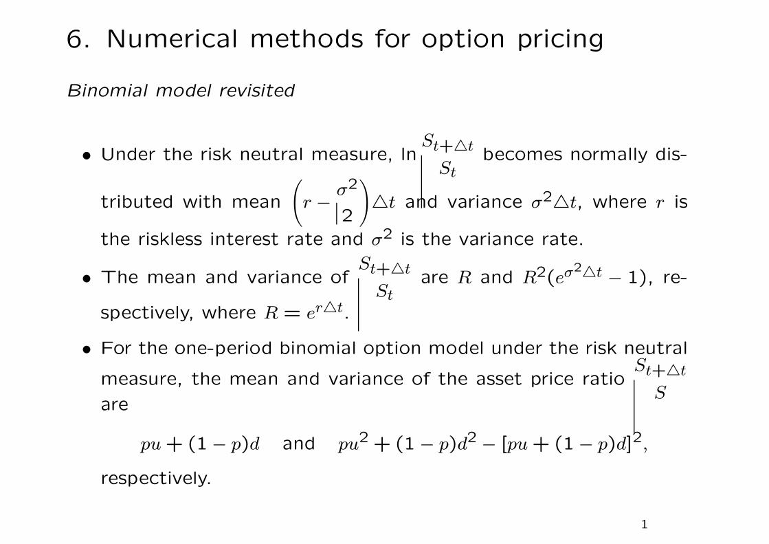
6. Numerical methods for option pricing

Binomial model revisited

• Under the risk neutral measure, lnSt+△t

Stbecomes normally dis-

tributed with mean

(r − σ2

2

)△t and variance σ2△t, where r is

the riskless interest rate and σ2 is the variance rate.

• The mean and variance ofSt+△t

Stare R and R2(eσ2△t − 1), re-

spectively, where R = er△t.

• For the one-period binomial option model under the risk neutral

measure, the mean and variance of the asset price ratioSt+△t

Sare

pu + (1 − p)d and pu2 + (1 − p)d2 − [pu + (1 − p)d]2,

respectively.

1

• By equating the mean and variance of the asset price ratio in

both continuous and discrete models, we obtain

pu + (1 − p)d = R

pu2 + (1 − p)d2 − R2 = R2(eσ2△t − 1).

The first equation leads to p =R − d

u − d, the usual risk neutral

probability.

• A convenient choice of the third condition is the tree-symmetry

condition

u =1

d,

so that the lattice nodes associated with the binomial tree are

symmetrical. Writing σ2 = R2eσ2△t, the solution is found to be

u =1

d=

σ2 + 1 +√

(σ2 + 1)2 − 4R2

2R, p =

R − d

u − d.

2

• By expanding u in Taylor series in powers of√△t, we obtain

u = 1 + σ√△t +

σ2

2△t +

4r2 + 4σ2r + 3σ4

8σ△t

32 + O(△t2).

• Observe that the first three terms in the above Taylor series

agree with those of eσ√△t up to O(△t) term.

• This suggests the judicious choice of the following set of pa-

rameter values

u = eσ√△t, d = e−σ

√△t, p =

R − d

u − d.

• With this new set of parameters, the variance of the price ratioSt+△t

Stin the continuous and discrete models agree up to O(△t).

3

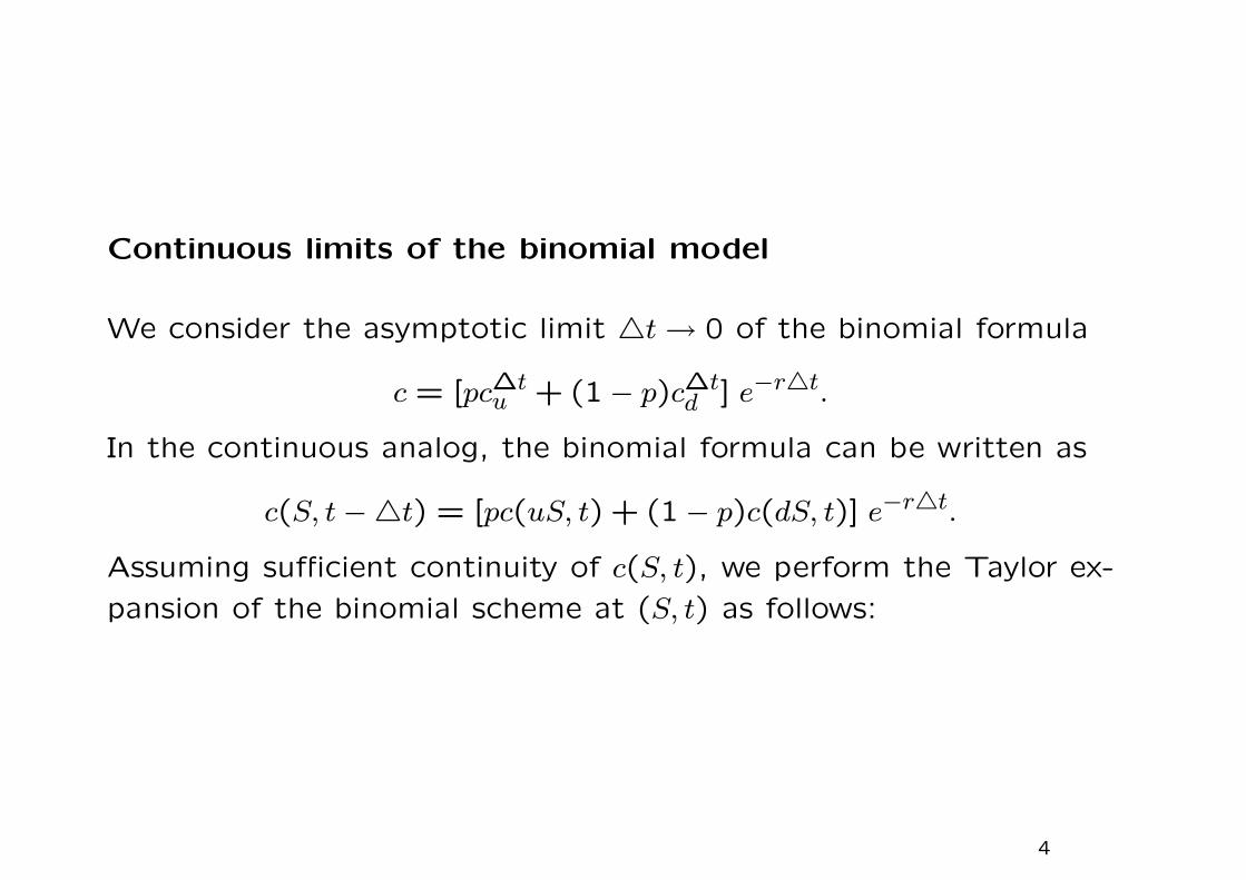
Continuous limits of the binomial model

We consider the asymptotic limit △t → 0 of the binomial formula

c = [pc∆tu + (1 − p)c∆t

d ] e−r△t.

In the continuous analog, the binomial formula can be written as

c(S, t −△t) = [pc(uS, t) + (1 − p)c(dS, t)] e−r△t.

Assuming sufficient continuity of c(S, t), we perform the Taylor ex-

pansion of the binomial scheme at (S, t) as follows:

4

−c(S, t −△t) + [pc(uS, t) + (1 − p)c(dS, t)]e−r△t

=∂c

∂t(S, t)△t − 1

2

∂2c

∂t2(S, t)△t2 + · · · − (1 − e−r△t)c(S, t)

+ e−r△t{[p(u − 1) + (1 − p)(d − 1)]S

∂c

∂S(S, t)

+1

2[p(u − 1)2 + (1 − p)(d − 1)2]S2 ∂2c

∂S2(S, t)

+1

6[p(u − 1)3 + (1 − p)(d − 1)3]S3 ∂3c

∂S3(S, t) + · · ·

}.

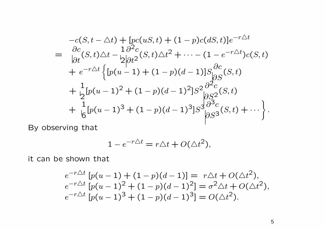
By observing that

1 − e−r△t = r△t + O(△t2),

it can be shown that

e−r△t [p(u − 1) + (1 − p)(d − 1)] = r△t + O(△t2),

e−r△t [p(u − 1)2 + (1 − p)(d − 1)2] = σ2△t + O(△t2),

e−r△t [p(u − 1)3 + (1 − p)(d − 1)3] = O(△t2).

5

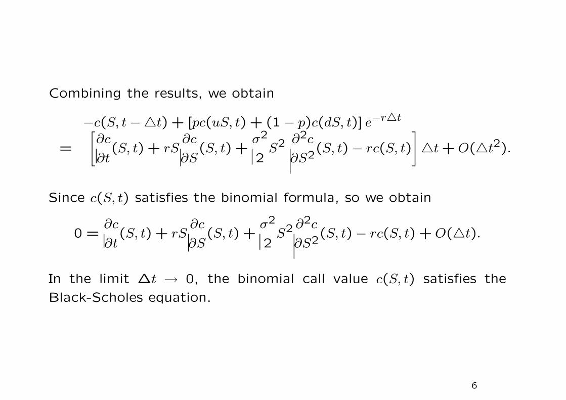
Combining the results, we obtain

−c(S, t −△t) + [pc(uS, t) + (1 − p)c(dS, t)] e−r△t

=

[∂c

∂t(S, t) + rS

∂c

∂S(S, t) +

σ2

2S2 ∂2c

∂S2(S, t) − rc(S, t)

]△t + O(△t2).

Since c(S, t) satisfies the binomial formula, so we obtain

0 =∂c

∂t(S, t) + rS

∂c

∂S(S, t) +

σ2

2S2 ∂2c

∂S2(S, t) − rc(S, t) + O(△t).

In the limit ∆t → 0, the binomial call value c(S, t) satisfies the

Black-Scholes equation.

6

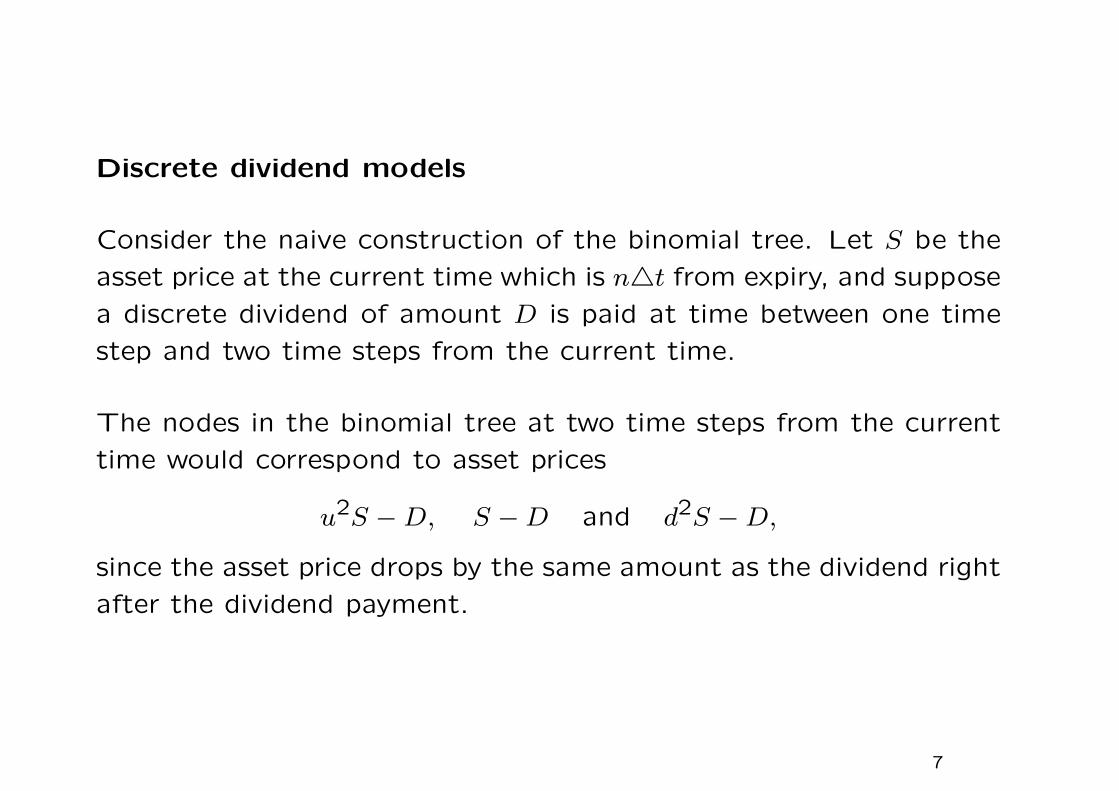
Discrete dividend models

Consider the naive construction of the binomial tree. Let S be the

asset price at the current time which is n△t from expiry, and suppose

a discrete dividend of amount D is paid at time between one time

step and two time steps from the current time.

The nodes in the binomial tree at two time steps from the current

time would correspond to asset prices

u2S − D, S − D and d2S − D,

since the asset price drops by the same amount as the dividend right

after the dividend payment.

7

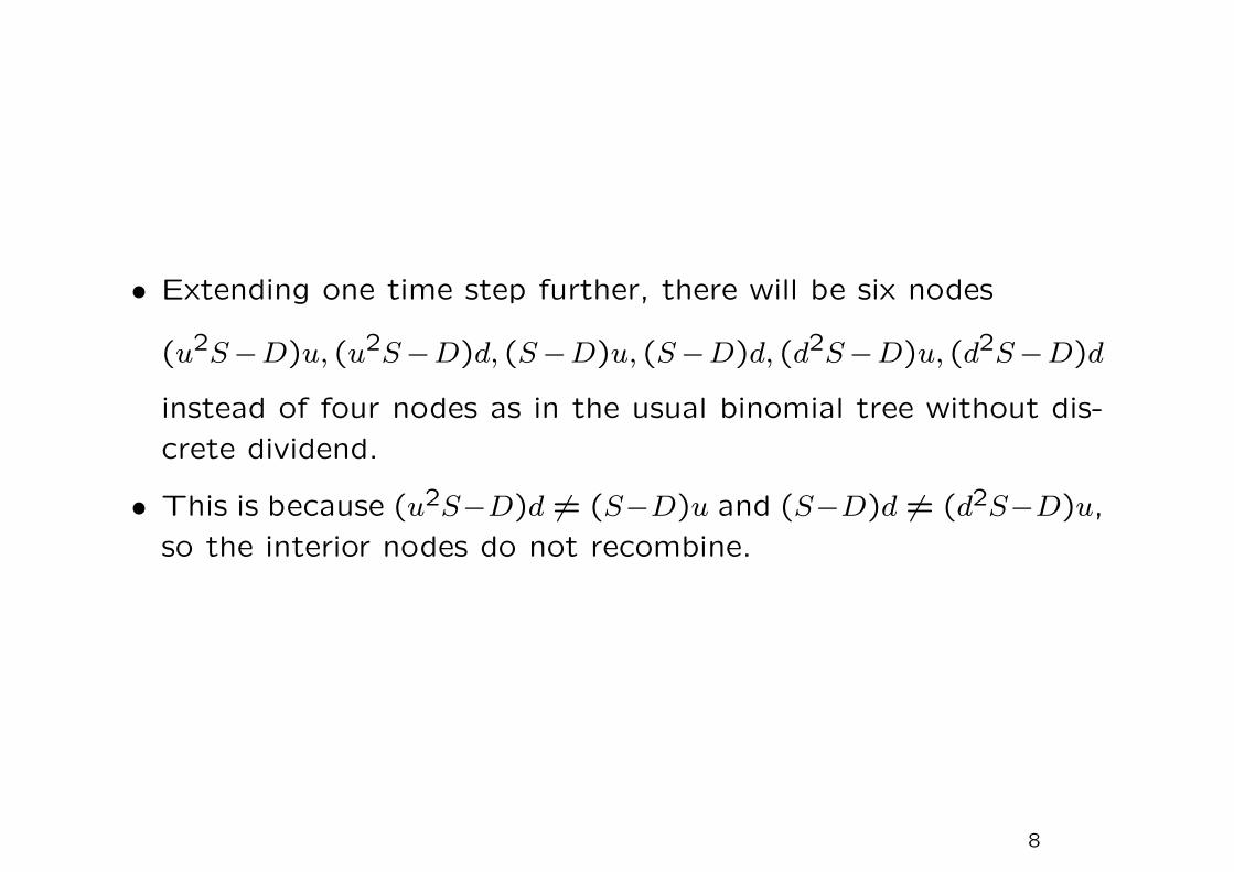
• Extending one time step further, there will be six nodes

(u2S−D)u, (u2S−D)d, (S−D)u, (S−D)d, (d2S−D)u, (d2S−D)d

instead of four nodes as in the usual binomial tree without dis-

crete dividend.

• This is because (u2S−D)d 6= (S−D)u and (S−D)d 6= (d2S−D)u,

so the interior nodes do not recombine.

8

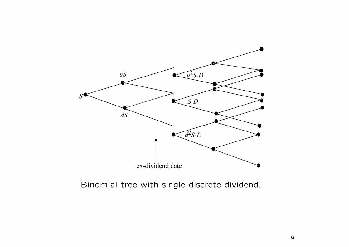
Binomial tree with single discrete dividend.

9

• Splitting the asset price St into two parts: the risky component

St that is stochastic and the remaining part that will be used to

pay the discrete dividend (assumed to be deterministic) in the

future.

• Suppose the dividend date is t∗, then at the current time t, the

risky component St is given by

St =

{St − De−r(t∗−t), t < t∗St, t > t∗.

• Let σ denote the volatility of St and assume σ to be constant

rather than the volatility of St itself to be constant.

10

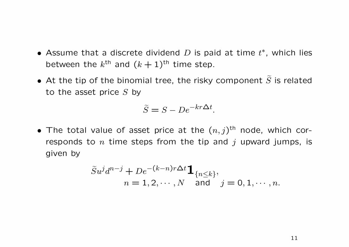
• Assume that a discrete dividend D is paid at time t∗, which lies

between the kth and (k + 1)th time step.

• At the tip of the binomial tree, the risky component S is related

to the asset price S by

S = S − De−kr∆t.

• The total value of asset price at the (n, j)th node, which cor-

responds to n time steps from the tip and j upward jumps, is

given by

Sujdn−j + De−(k−n)r∆t1{n≤k},n = 1,2, · · · , N and j = 0,1, · · · , n.

11

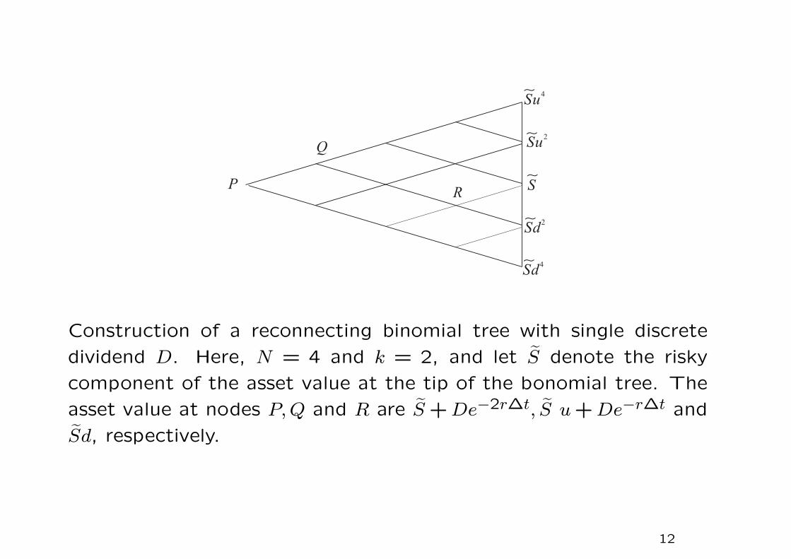
Construction of a reconnecting binomial tree with single discrete

dividend D. Here, N = 4 and k = 2, and let S denote the risky

component of the asset value at the tip of the bonomial tree. The

asset value at nodes P, Q and R are S + De−2r∆t, S u + De−r∆t and

Sd, respectively.

12

Early exercise feature and callable feature

• Without the early exercise privilege, risk neutral valuation leads

to the usual binomial formula

Vcont =pV ∆t

u + (1 − p)V ∆td

R.

• The following simple dynamic programming procedure is applied

at each binomial node

V = max(Vcont, h(S)),

where h(S) is the exercise payoff when the asset price assumes

the value S.

13

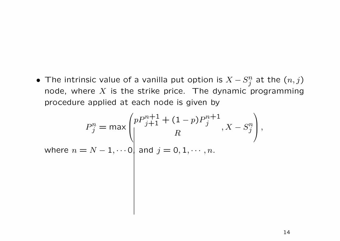
• The intrinsic value of a vanilla put option is X −Snj at the (n, j)

node, where X is the strike price. The dynamic programming

procedure applied at each node is given by

Pnj = max

pPn+1j+1 + (1 − p)Pn+1

j

R, X − Sn

j

,

where n = N − 1, · · ·0, and j = 0,1, · · · , n.

14

Callable American call

• The callable feature entitles the issuer to buy back the American

option at any time at a predetermined call price.

• Upon call, the holder can choose either to exercise the call or

receive the call price as cash.

• Let the call price be K. The dynamic programming procedure

applied at each node is modified as follows

Cnj = min

max

pcn+1j+1 + (1 − p)cn+1

j

R, Sn

j − X

,

max(K, Snj − X)

.

15

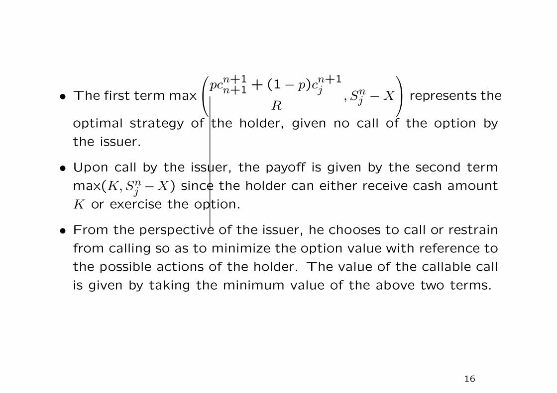
• The first term max

pcn+1n+1 + (1 − p)cn+1

j

R, Sn

j − X

represents the

optimal strategy of the holder, given no call of the option by

the issuer.

• Upon call by the issuer, the payoff is given by the second term

max(K, Snj −X) since the holder can either receive cash amount

K or exercise the option.

• From the perspective of the issuer, he chooses to call or restrain

from calling so as to minimize the option value with reference to

the possible actions of the holder. The value of the callable call

is given by taking the minimum value of the above two terms.

16

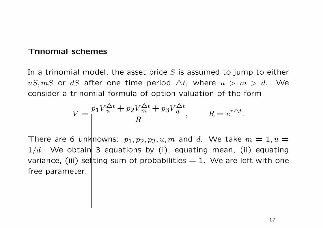
Trinomial schemes

In a trinomial model, the asset price S is assumed to jump to either

uS, mS or dS after one time period △t, where u > m > d. We

consider a trinomial formula of option valuation of the form

V =p1V ∆t

u + p2V ∆tm + p3V ∆t

d

R, R = er△t.

There are 6 unknowns: p1, p2, p3, u, m and d. We take m = 1, u =

1/d. We obtain 3 equations by (i), equating mean, (ii) equating

variance, (iii) setting sum of probabilities = 1. We are left with one

free parameter.

17

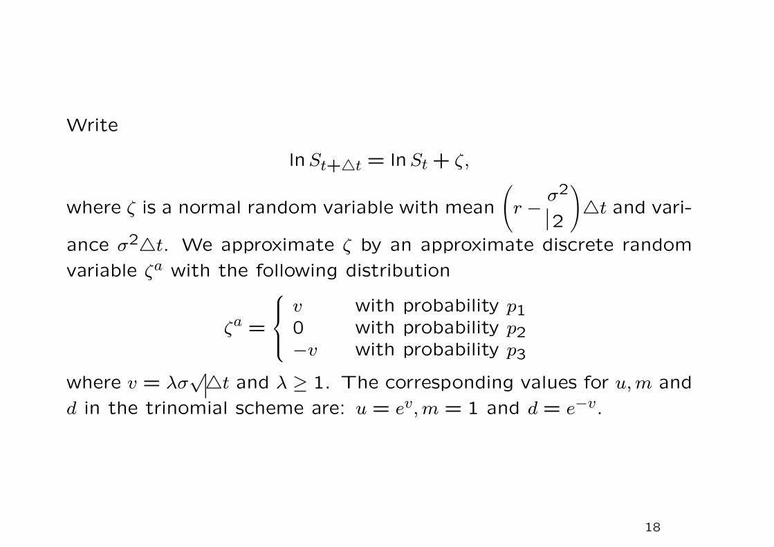
Write

lnSt+△t = lnSt + ζ,

where ζ is a normal random variable with mean

(r − σ2

2

)△t and vari-

ance σ2△t. We approximate ζ by an approximate discrete random

variable ζa with the following distribution

ζa =

v with probability p10 with probability p2−v with probability p3

where v = λσ√△t and λ ≥ 1. The corresponding values for u, m and

d in the trinomial scheme are: u = ev, m = 1 and d = e−v.

18

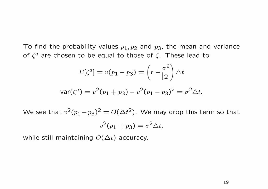
To find the probability values p1, p2 and p3, the mean and variance

of ζa are chosen to be equal to those of ζ. These lead to

E[ζa] = v(p1 − p3) =

(r − σ2

2

)△t

var(ζa) = v2(p1 + p3) − v2(p1 − p3)2 = σ2△t.

We see that v2(p1−p3)2 = O(∆t2). We may drop this term so that

v2(p1 + p3) = σ2△t,

while still maintaining O(∆t) accuracy.

19

Lastly, the probabilities must be summed to one so that

p1 + p2 + p3 = 1.

We then solve together to obtain

p1 =1

2λ2+

(r − σ2

2 )√△t

2λσ

p2 = 1 − 1

λ2

p3 =1

2λ2−

(r − σ2

2 )√△t

2λσ,

here λ is a free parameter.

20

Multi-state options

• We assume the joint density of the prices of the two underlying

assets S1 and S2 to be bivariate lognormal.

• Let σi be the volatility of asset price Si, i = 1,2 and ρ be

the correlation coefficient between the two lognormal diffusion

processes.

• Let Si and S△ti denote, respectively, the price of asset i at the

current time and one period △t later.

• Under the risk neutral measure, we have

lnS△ti

Si= ζi, i = 1,2,

where ζi is a normal random variable with mean

(r − σ2

i

2

)△t and

variance σ2i △t.

21

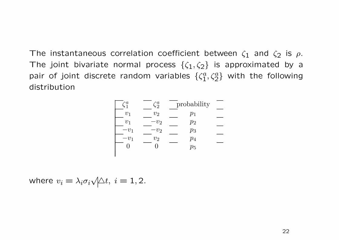
The instantaneous correlation coefficient between ζ1 and ζ2 is ρ.

The joint bivariate normal process {ζ1, ζ2} is approximated by a

pair of joint discrete random variables {ζa1, ζa

2} with the following

distribution { 1 2 }

ζa

1ζa

2probability

v1 v2 p1

v1 −v2 p2

−v1 −v2 p3

−v1 v2 p4

0 0 p5

where vi = λiσi√△t, i = 1,2.

22

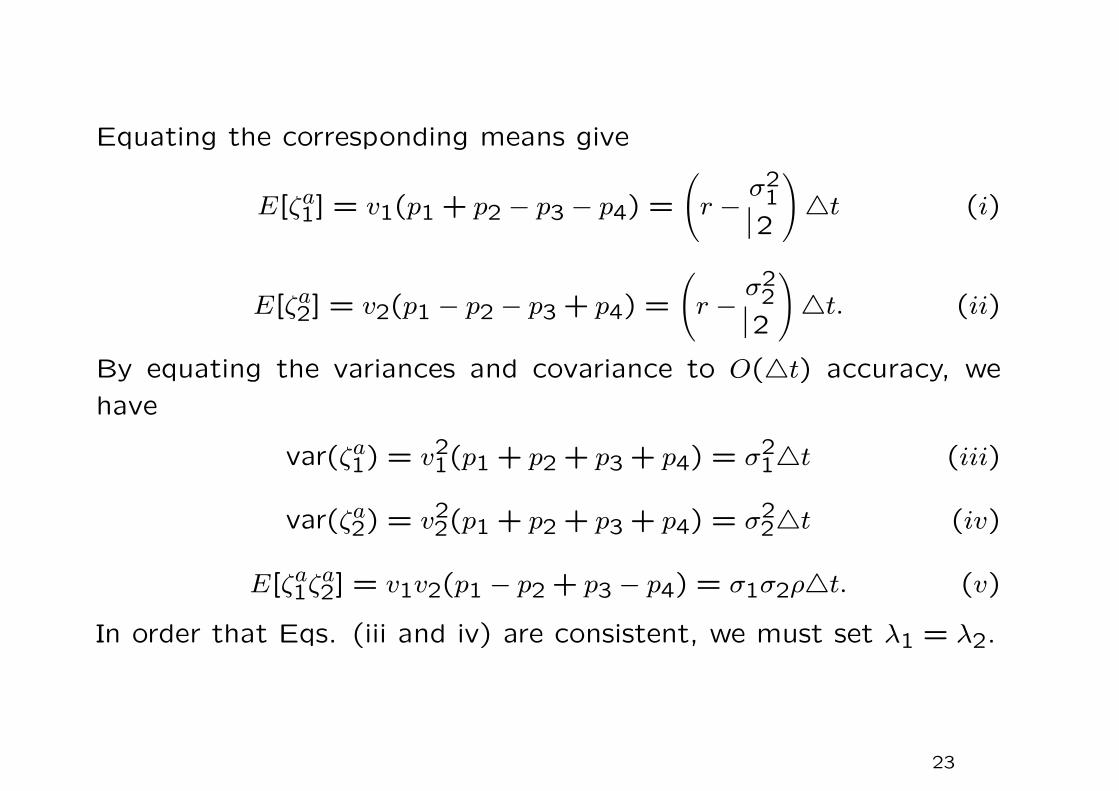
Equating the corresponding means give

E[ζa1] = v1(p1 + p2 − p3 − p4) =

(r − σ2

1

2

)△t (i)

E[ζa2] = v2(p1 − p2 − p3 + p4) =

(r − σ2

2

2

)△t. (ii)

By equating the variances and covariance to O(△t) accuracy, we

have

var(ζa1) = v2

1(p1 + p2 + p3 + p4) = σ21△t (iii)

var(ζa2) = v2

2(p1 + p2 + p3 + p4) = σ22△t (iv)

E[ζa1ζa

2] = v1v2(p1 − p2 + p3 − p4) = σ1σ2ρ△t. (v)

In order that Eqs. (iii and iv) are consistent, we must set λ1 = λ2.

23

Writing λ = λ1 = λ2, we have the following four independent equa-

tions for the five probability values

p1 + p2 − p3 − p4 =(r − σ2

12 )

√△t

λσ1

p1 − p2 − p3 + p4 =(r − σ2

22 )

√△t

λσ2

p1 + p2 + p3 + p4 =1

λ2

p1 − p2 + p3 − p4 =ρ

λ2.

Since the probabilities must be summed to one, this gives the re-

maining condition as

p1 + p2 + p3 + p4 + p5 = 1.

24

The solution of the above linear algebraic system of equations gives

p1 =1

4

1

λ2+

√△t

λ

r − σ212

σ1+

r − σ222

σ2

+

ρ

λ2

p2 =1

4

1

λ2+

√△t

λ

r − σ212

σ1−

r − σ222

σ2

− ρ

λ2

p3 =1

4

1

λ2+

√△t

λ

−

r − σ212

σ1−

r − σ222

σ2

+

ρ

λ2

p4 =1

4

1

λ2+

√△t

λ

−

r − σ212

σ1+

r − σ222

σ2

− ρ

λ2

p5 = 1 − 1

λ2, λ ≥ 1 is a free parameter.

25

Two-state trinomial model

• For convenience, we write ui = evi, di = e−vi, i = 1,2.

• Let V ∆tu1u2

denote the option price at one time period later with

asset prices u1S1 and u2S2, and similar meaning for V ∆tu1d2

, V ∆td1u2

and V ∆td1d2

.

• We let V ∆t0,0 denote the option price one period later with no

jumps in asset prices.

• The corresponding 5-point formula for the two-state trinomial

model can be expressed as

V = (p1V △tu1u2

+ p2V△tu1d2

+ p3V△td1d2

+ p4V△td1u2

+ p5V△t0,0)/R.

• When λ = 1, we have p5 = 0 and the above 5-point formula

reduces to the 4-point formula.

26

Forward shooting grid methods

• For path dependent options, the option value also depends on

the path function Ft = F(S, t) defined specifically for the given

nature of path dependence, say, the minimum asset price realized

along a specific asset price path.

• Since option value depends also on Ft, we find the value of the

path dependent option at each node in the lattice tree for all

alternative values of Ft that can occur.

• The approach of appending an auxiliary state vector at each

node in the lattice tree to model the correlated evolution of

Ft with St is commonly called the forward shooting grid (FSG)

method.

27

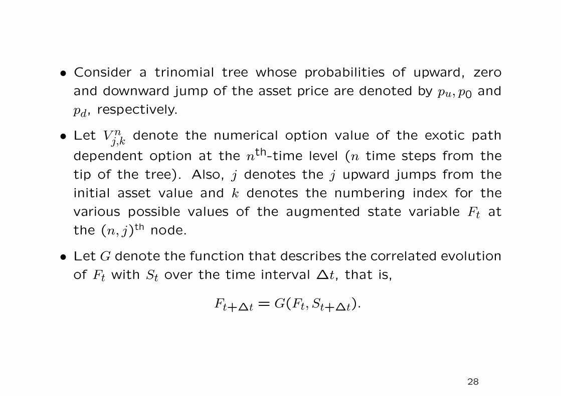
• Consider a trinomial tree whose probabilities of upward, zero

and downward jump of the asset price are denoted by pu, p0 and

pd, respectively.

• Let V nj,k denote the numerical option value of the exotic path

dependent option at the nth-time level (n time steps from the

tip of the tree). Also, j denotes the j upward jumps from the

initial asset value and k denotes the numbering index for the

various possible values of the augmented state variable Ft at

the (n, j)th node.

• Let G denote the function that describes the correlated evolution

of Ft with St over the time interval ∆t, that is,

Ft+∆t = G(Ft, St+∆t).

28

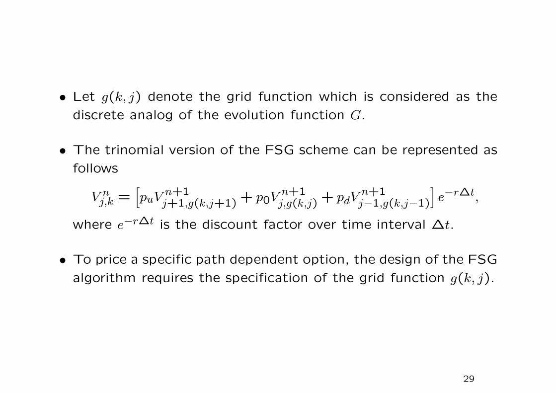
• Let g(k, j) denote the grid function which is considered as the

discrete analog of the evolution function G.

• The trinomial version of the FSG scheme can be represented as

follows

V nj,k =

[puV n+1

j+1,g(k,j+1)+ p0V n+1

j,g(k,j)+ pdV

n+1j−1,g(k,j−1)

]e−r∆t,

where e−r∆t is the discount factor over time interval ∆t.

• To price a specific path dependent option, the design of the FSG

algorithm requires the specification of the grid function g(k, j).

29

Cumulative Parisian feature

• Let M denote the prespecified number of cumulative breaching

occurrences that is required to activate knock-out, and let k be

the integer variable that counts the number of breaching so far.

• Let B denote the down barrier associated with the knock-out

feature.

• Let xj denote the value of x = lnS that corresponds to j upward

moves in the trinomial tree.

• When n∆t happens to be a monitoring instant, the index k

increases its value by 1 if the asset price S falls on or below the

barrier B, that is, xj ≤ lnB.

30

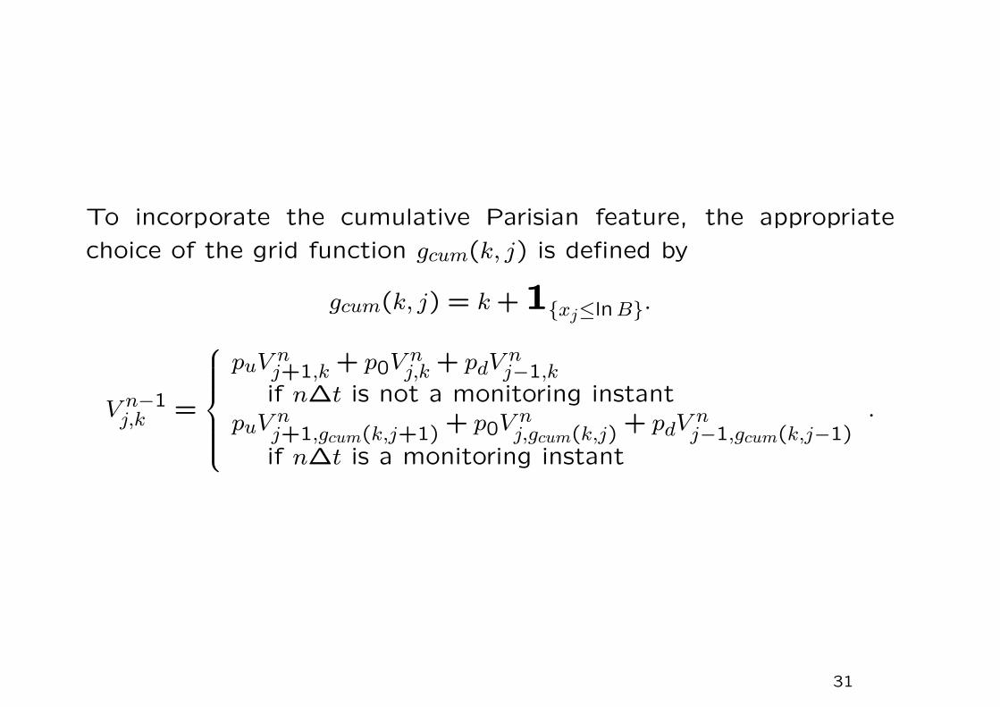
To incorporate the cumulative Parisian feature, the appropriate

choice of the grid function gcum(k, j) is defined by

gcum(k, j) = k +1{xj≤lnB}.

V n−1j,k =

puV nj+1,k + p0V n

j,k + pdVnj−1,k

if n∆t is not a monitoring instantpuV n

j+1,gcum(k,j+1)+ p0V n

j,gcum(k,j)+ pdV

nj−1,gcum(k,j−1)

if n∆t is a monitoring instant

.

31

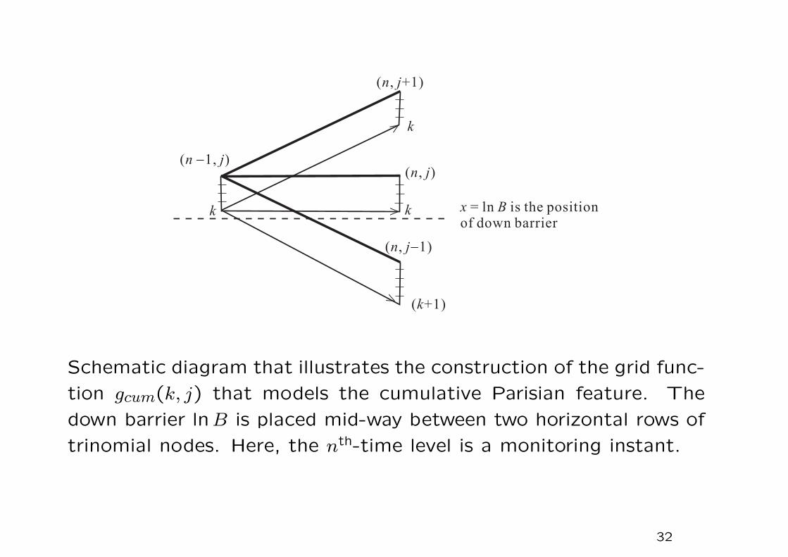
Schematic diagram that illustrates the construction of the grid func-

tion gcum(k, j) that models the cumulative Parisian feature. The

down barrier lnB is placed mid-way between two horizontal rows of

trinomial nodes. Here, the nth-time level is a monitoring instant.

32

Finite difference algorithms

Black-Scholes equation:∂V

∂t+ rS

∂V

∂S+

σ2

2S2∂2V

∂S2− rV = 0.

Use the transformed variables: τ = T − t, x = lnS,

∂

∂t= − ∂

∂τ,

∂

∂S=

1

S

∂

∂xor S

∂

∂S=

∂

∂x∂2

∂x2= S

∂

∂S

(S

∂

∂S

)= S2 ∂2

∂S2+ S

∂

∂Sso that S2 ∂2

∂S2=

∂2

∂x2− ∂

∂x.

Black-Scholes equation

∂V

∂τ=

σ2

2

∂2V

∂x2+

(r − σ2

2

)∂V

∂x− rV, τ > 0,−∞ < x < ∞.

33

Preliminary procedure

Transform the domain of the continuous problem

{(x, τ) : −∞ < x < ∞, τ ≥ 0}

into a discretized domain.

Infinite of x = lnS is approximated by a finite truncated interval

[M1, M2], M1 and M2 are sufficiently large. The discretized do-

main is overlaid with a uniform system of meshes (j∆x, n∆τ), j =

0,1, · · · , N + 1, n = 1,2, · · · , with (N + 1)∆x = M1 + M2.

Step width ∆x and time step ∆τ are independent. Option values

are computed only at the grid points.

34

xn = 0

n = 1

n = 2

-M1

j = 0

),( τ∆∆ nxj

∆x ∆τ

M2

j = N + 1

τ

Finite difference mesh with uniform stepwidth ∆x and time step

∆τ . Numerical option values are computed at the node points

(j∆x, n∆τ), j = 1,2, · · · , N , n = 1,2, · · · . Option values along the

boundaries: j = 0 and j = N + 1 are prescribed by the boundary

conditions of the option model. The “initial” values V 0j along the

zeroth time level, n = 0, are given by the terminal payoff function.

35

Let V nj denote the numerical approximation of V (j△x, n△τ). The

continuous temporal and spatial derivatives are approximated by the

following finite difference operators

∂V

∂τ(j△x, n△τ) ≈

V n+1j − V n

j

△τ(forward difference)

∂V

∂x(j△x, n△τ) ≈

V nj+1 − V n

j−1

2△x(centered difference)

∂2V

∂x2(j△x, n△τ) ≈

V nj+1 − 2V n

j + V nj−1

△x2(centered difference)

By taking

Wn+1j = er(n+1)∆τV n+1

j and Wnj = ern∆τV n

j ,

then canceling ern∆τ , we obtain the following explicit Forward-

Time-Centered-Space (FTCS) finite difference scheme

36

V n+1j =

[V n

j +σ2

2

△τ

△x2

(V n

j+1 − 2V nj + V n

j−1

)

+

(r − σ2

2

)△τ

2△x

(V n

j+1 − V nj−1

)]e−r△τ .

• Suppose we are given “initial” values V 0j , j = 0,1, · · · , N + 1

along the zeroth time level, we can use the explicit scheme to

find values V 1j , j = 1,2, · · · , N along the first time level τ = △τ .

• The values at the two ends V 10 and V 1

N+1 are given by the

numerical boundary conditions specified for the option model.

37

Two-level four-point explicit schemes

V n+1j = b1V n

j+1 + b0V nj + b−1V n

j−1, j = 1,2, · · · , N, n = 0,1,2, · · · .

The above FTCS scheme corresponds to

b1 =

[σ2

2

△τ

△x2+

(r − σ2

2

)△τ

2△x

]e−r∆τ ,

b0 =

[1 − σ2 △τ

△x2

]e−r∆τ ,

b−1 =

[σ2

2

△τ

△x2−(

r − σ2

2

)△τ

2△x

]er∆τ .

Both the binomial and trinomial schemes are members of the family

when the reconnecting condition ud = 1 holds.

38

Suppose we write △x = lnu, then ln d = −△x; the binomial scheme

can be expressed as

V n+1(x) =pV n(x + △x) + (1 − p)V n(x −△x)

R, x = lnS, and R = er△τ ,

where V n+1(x), V n(x +△x) and V n(x−△x) are analogous to c, c∆tu

and c∆td , respectively. The corresponds to

b1 = p/R, b0 = 0 and b−1 = (1 − p)/R.

In the Cox-Ross-Rubinstein scheme, they are related by ∆x = lnu =

σ√

∆τ or σ2∆τ = ∆x2. In the trinomial scheme, their relation is

given by λ2σ2∆τ = ∆x2, where the free parameter λ can be chosen

arbitrarily.

39

Numerical stability and oscillation phenomena

• A numerical scheme must be consistent in order that the numer-

ical solution converges to the exact solution of the underlying

differential equation. However, consistency is only a necessary

but not sufficient condition for convergence.

• The roundoff errors incurred during numerical calculations may

lead to the blow up of the solution and erode the whole com-

putation.

40

Order of accuracy

Suppose the leading truncation terms are O(∆τk,∆xm), then the

numerical scheme is said to be kth order time accurate and mth

order space accurate. The explicit FTCS scheme is first order time

accurate and second order space accurate. Suppose we choose ∆τ

to be the same order as ∆x2, that is, ∆τ = λ∆x2 for some finite

constant λ, then the leading truncation error terms become O(∆τ).

41

• A necessary condition for the convergence of the numerical so-

lution to the continuous solution is that the local truncation

error of the numerical scheme must tend to zero for vanishing

stepwidth and time step. In this case, the numerical scheme is

said to be consistent.

• The order of accuracy of a scheme is defined to be the order in

powers of ∆x and ∆τ in the leading truncation error terms.

42

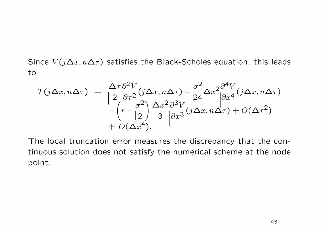
Since V (j∆x, n∆τ) satisfies the Black-Scholes equation, this leads

to

T(j∆x, n∆τ) =∆τ

2

∂2V

∂τ2(j∆x, n∆τ) − σ2

24∆x2∂4V

∂x4(j∆x, n∆τ)

−(

r − σ2

2

)∆x2

3

∂3V

∂x3(j∆x, n∆τ) + O(∆τ2)

+ O(∆x4).

The local truncation error measures the discrepancy that the con-

tinuous solution does not satisfy the numerical scheme at the node

point.

43

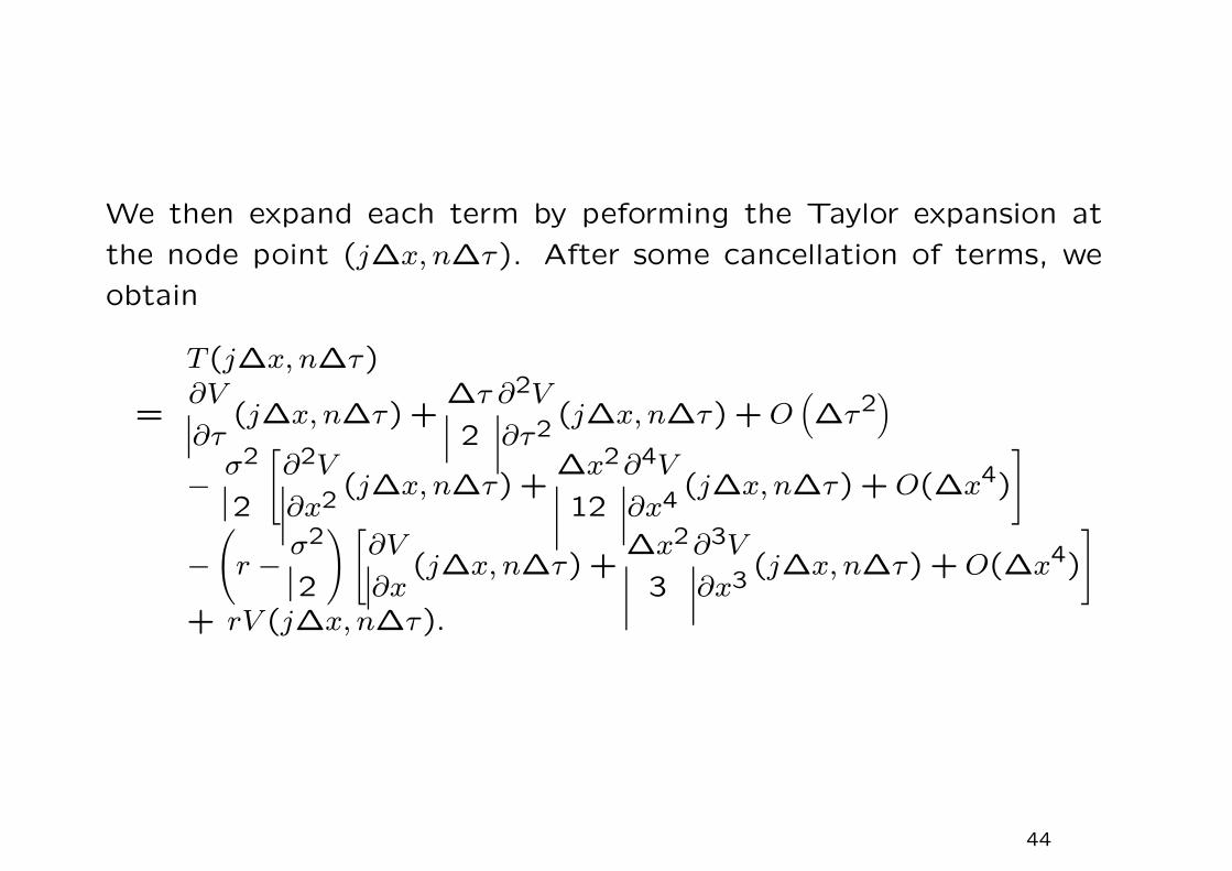
We then expand each term by peforming the Taylor expansion at

the node point (j∆x, n∆τ). After some cancellation of terms, we

obtain

T(j∆x, n∆τ)

=∂V

∂τ(j∆x, n∆τ) +

∆τ

2

∂2V

∂τ2(j∆x, n∆τ) + O

(∆τ2

)

− σ2

2

[∂2V

∂x2(j∆x, n∆τ) +

∆x2

12

∂4V

∂x4(j∆x, n∆τ) + O(∆x4)

]

−(

r − σ2

2

)[∂V

∂x(j∆x, n∆τ) +

∆x2

3

∂3V

∂x3(j∆x, n∆τ) + O(∆x4)

]

+ rV (j∆x, n∆τ).

44

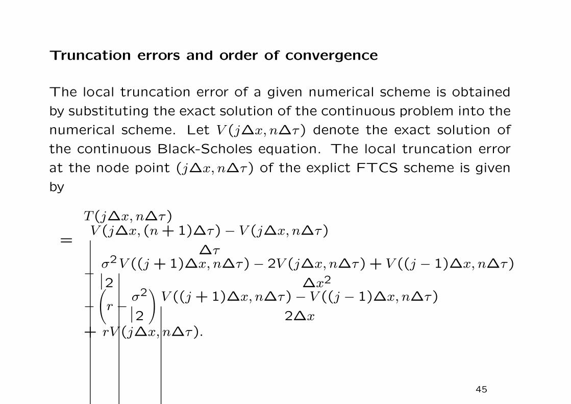
Truncation errors and order of convergence

The local truncation error of a given numerical scheme is obtained

by substituting the exact solution of the continuous problem into the

numerical scheme. Let V (j∆x, n∆τ) denote the exact solution of

the continuous Black-Scholes equation. The local truncation error

at the node point (j∆x, n∆τ) of the explict FTCS scheme is given

by

T(j∆x, n∆τ)

=V (j∆x, (n + 1)∆τ) − V (j∆x, n∆τ)

∆τ

− σ2

2

V ((j + 1)∆x, n∆τ) − 2V (j∆x, n∆τ) + V ((j − 1)∆x, n∆τ)

∆x2

−(

r − σ2

2

)V ((j + 1)∆x, n∆τ) − V ((j − 1)∆x, n∆τ)

2∆x+ rV (j∆x, n∆τ).

45

Monte Carlo simulation

A wide class of derivative pricing problems come down to the eval-

uation of the following expectation functional

Ef [Z(T ; t, z)].

• Z denotes the stochastic process that describes the price evolu-

tion of one or more underlying financial variables such as asset

prices and interest rates, under the respective risk neutral prob-

ability distributions.

• The process Z has the initial value z at time t, and the function

f specifies the value of the derivative at the expiration time T .

46

• The Monte Carlo method is basically a numerical procedure for

estimating the expected value of a random variable,a nd so it

leads itself naturally to derivative pricing problem represented as

expectations.

• The simulation procedure involves generating random variables

with a given probability density and using the law of large num-

bers to take the average of these values as an estimate of the

expected value of the random variable.

47

In the context of derivative pricing, the Monte Carlo procedure in-

volves the following steps.

(i) Simulate sample paths of the underlying state variables in the

derivative model such as asset prices and interest rates over the

life of the derivative, according to the risk neutral probability

distributions.

(ii) For each simulated sample path, evaluate the discounted cash

flows of the derivative.

(iii) Take the sample average of the discounted cash flows over all

sample paths.

48

• The numerical procedure requires the computation of the ex-

pected payoff of the call option at expiry, Et[max(ST − X,0)],

and discounted to the present value at time t, namely, e−r(T−t)

Et[max(ST − X,0)].

• Assuming lognormal distribution for the asset price movement,

the price dynamics under the risk neutral measure is given by

St+△t

St= e

(r−σ2

2

)∆t+σǫ

√∆t

,

where ∆t is the time step, σ is the volatility and r is the riskless

interest rate.

49

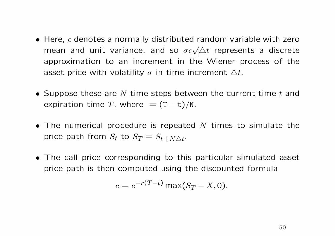
• Here, ǫ denotes a normally distributed random variable with zero

mean and unit variance, and so σǫ√△t represents a discrete

approximation to an increment in the Wiener process of the

asset price with volatility σ in time increment △t.

• Suppose these are N time steps between the current time t and

expiration time T , where = (T− t)/N.

• The numerical procedure is repeated N times to simulate the

price path from St to ST = St+N△t.

• The call price corresponding to this particular simulated asset

price path is then computed using the discounted formula

c = e−r(T−t) max(ST − X,0).

50

• After repeating the above simulation for a sufficiently large num-

ber of runs, the expected call value is obtained by computing the

average of the estimates of the call value found in the sample

simulation.

• Let ci denote the estimate of the call value obtained in the ith

simulation and M be the total number of simulation runs.

• The expected call value is given by

c =1

M

M∑

i=1

ci,

and the variance of the estimate is computed by

s2 =1

M − 1

M∑

i=1

(ci − c)2.

51

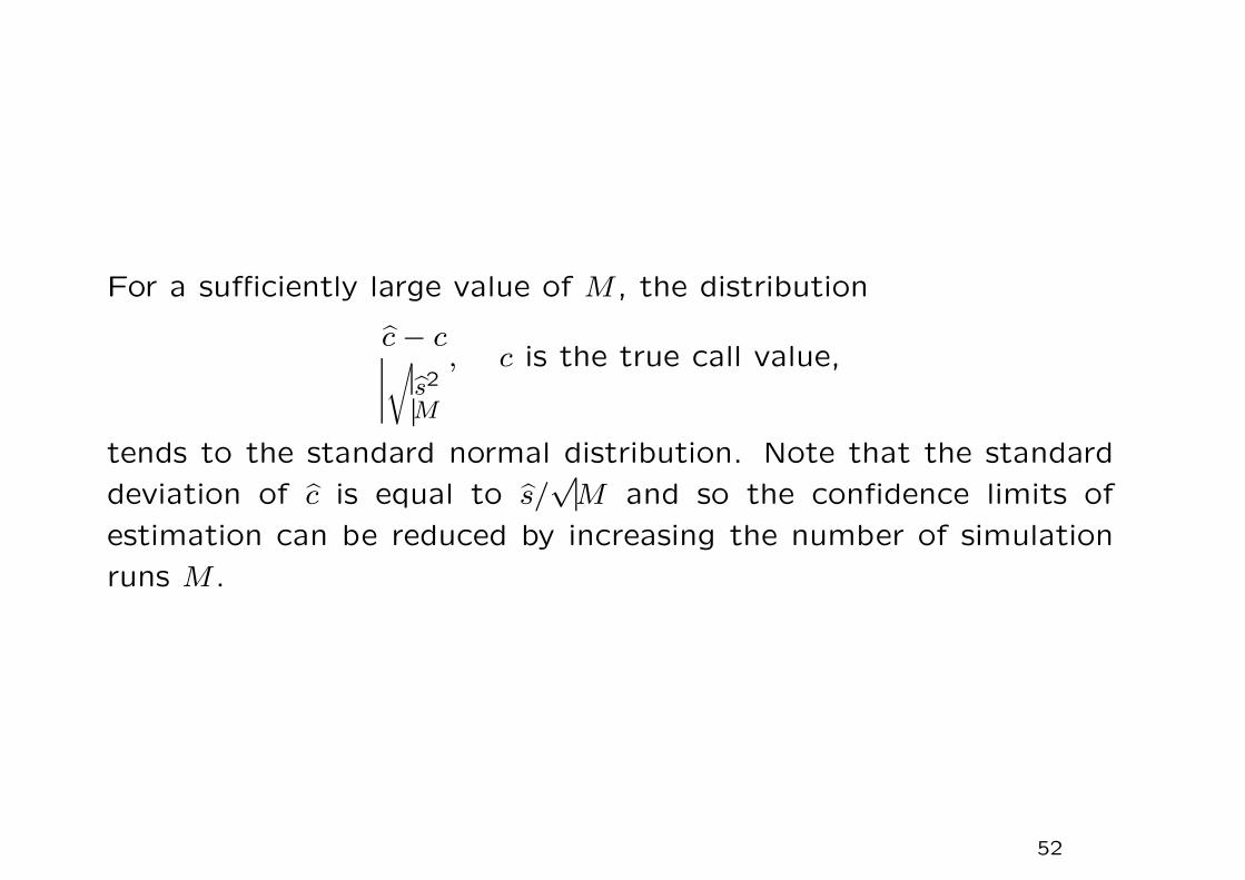
For a sufficiently large value of M , the distribution

c − c√

s2

M

, c is the true call value,

tends to the standard normal distribution. Note that the standard

deviation of c is equal to s/√

M and so the confidence limits of

estimation can be reduced by increasing the number of simulation

runs M .

52

Advantages

1. The error is independent of the dimension of the option problem.

2. Its ease to accommodate complicated payoff in an option model.

For example, the terminal payoff of an Asian option depends on

the average of the asset price over certain time interval while

that of a lookback option depends on the extremum value of the

asset price over some period of time. It is quite straightforward

to obtain the average or extremum value in the simulated price

path in each simulated path.

Drawback

The demand for a large number of simulation trials in order to

achieve a high level of accuracy.

53

Computational efficiency

• Suppose WT is the total amount of computational work units

available to generate an estimate of the value of an option V .

• Assume that there are two methods for generating the Monte

Carlo estimates for the option value, requiring W1 and W2 units

of computation work respectively for each simulation run. For

simplicity, assume WT is divisible by both W1 and W2.

54

• Let V(1)i and V

(2)i denote the estimator of V in the ith simula-

tion using Methods 1 and 2, respectively, and their respective

standard deviations are σ1 and σ2.

• The sample means for estimating V from the two methods using

WT amount of work are, respectively,

W1

WT

WT/W1∑

i=1

V(1)i and

W2

WT

WT/W2∑

i=1

V(2)i .

55

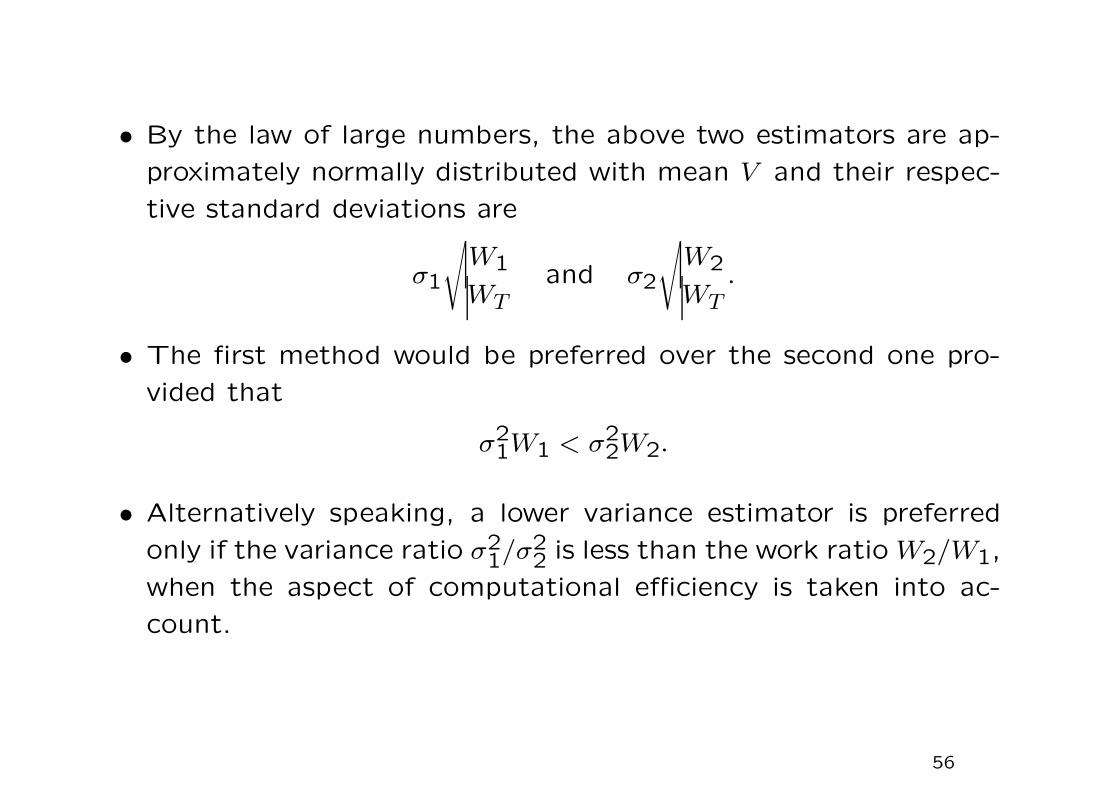
• By the law of large numbers, the above two estimators are ap-

proximately normally distributed with mean V and their respec-

tive standard deviations are

σ1

√W1

WTand σ2

√W2

WT.

• The first method would be preferred over the second one pro-

vided that

σ21W1 < σ2

2W2.

• Alternatively speaking, a lower variance estimator is preferred

only if the variance ratio σ21/σ2

2 is less than the work ratio W2/W1,

when the aspect of computational efficiency is taken into ac-

count.

56

Antithetic variates method

• Suppose {ǫ(i)} denotes the independent samples from the stan-

dard normal distribution for the ith simulation run of the asset

price path so that

S(i)T = St e

(r−σ2

2

)(T−t)+σ

√△tN∑

j=1ǫ(i)j

, i = 1,2, · · · , M,

where △t =T − t

Nand M is the total number of simulation runs.

Note that ǫ(i)j is randomly sampled from the standard normal

distribution.

• An unbiased estimator of the price of a European call option

with strike price X is given by

c =1

M

M∑

i=1

ci =1

M

M∑

i=1

e−r(T−t) max(S(i)T − X,0).

57

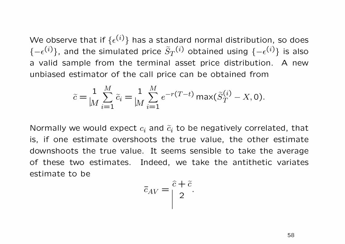
We observe that if {ǫ(i)} has a standard normal distribution, so does

{−ǫ(i)}, and the simulated price ST(i) obtained using {−ǫ(i)} is also

a valid sample from the terminal asset price distribution. A new

unbiased estimator of the call price can be obtained from

c =1

M

M∑

i=1

ci =1

M

M∑

i=1

e−r(T−t) max(S(i)T − X,0).

Normally we would expect ci and ci to be negatively correlated, that

is, if one estimate overshoots the true value, the other estimate

downshoots the true value. It seems sensible to take the average

of these two estimates. Indeed, we take the antithetic variates

estimate to be

cAV =c + c

2.

58

Control variate method

• The control variate method is applicable when there are two

similar options, A and B. Option A is the one whose price value

is desired, while option B is similar to option A in nature but its

analytic price formula is available.

• Let VA and VB denote the true value of option A and option B

respectively, and let VA and VB denote the respective estimated

value of option A and option B using the Monte Carlo simulation.

• How does the knowledge of VB and VB help improve the estimate

of the value of option A beyond the available estimate VA?

59

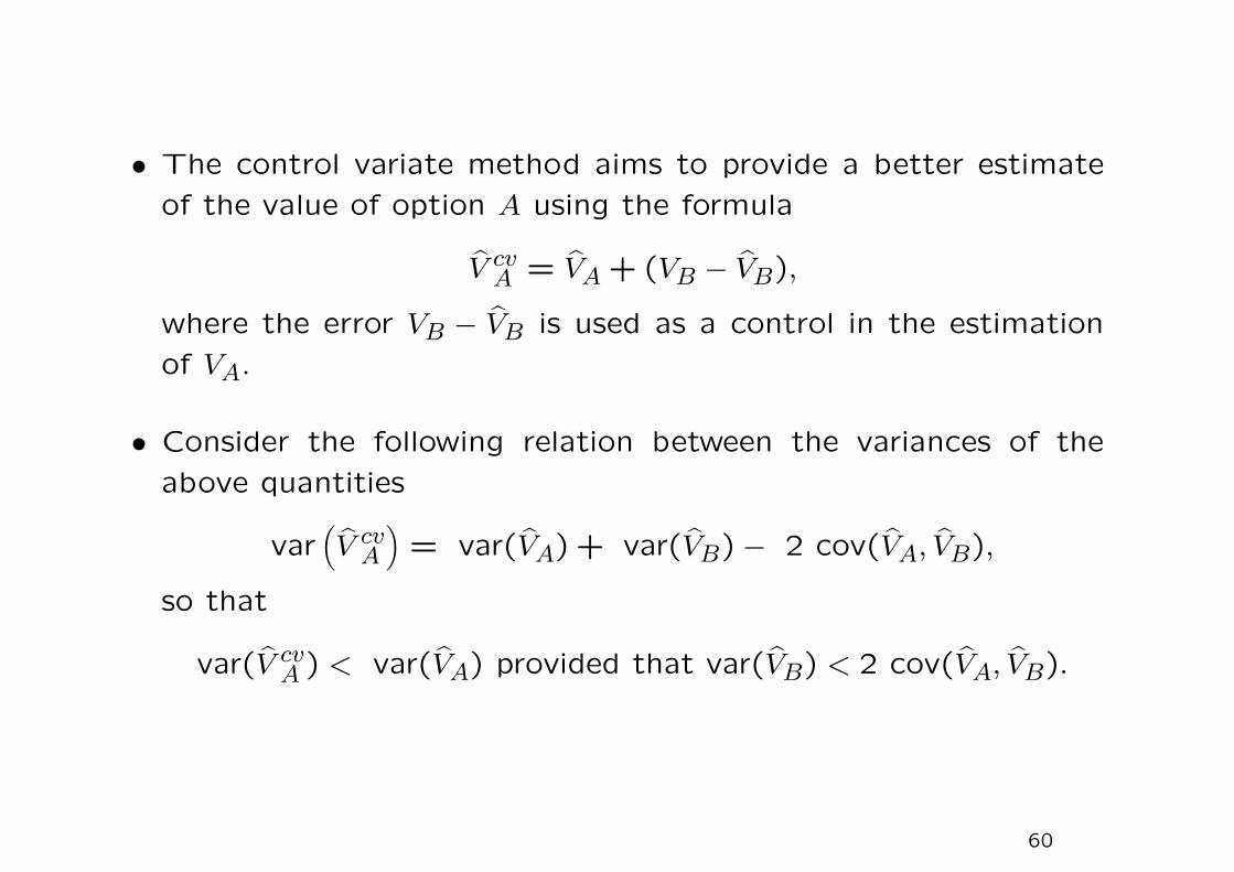
• The control variate method aims to provide a better estimate

of the value of option A using the formula

V cvA = VA + (VB − VB),

where the error VB − VB is used as a control in the estimation

of VA.

• Consider the following relation between the variances of the

above quantities

var(V cv

A

)= var(VA) + var(VB) − 2 cov(VA, VB),

so that

var(V cvA ) < var(VA) provided that var(VB) < 2 cov(VA, VB).

60

• The control variate technique reduces the variance of the esti-

mator of VA when the covariance between VA and VB is large.

This is true when the two options are strongly correlated.

• In terms of computational efforts, we need to compute two

estimates VA and VB.

• However, if the underlying asset price paths of the two options

are identical, then there is only slight additional work to evaluate

VB along with VA on the same set of simulated price paths.

61

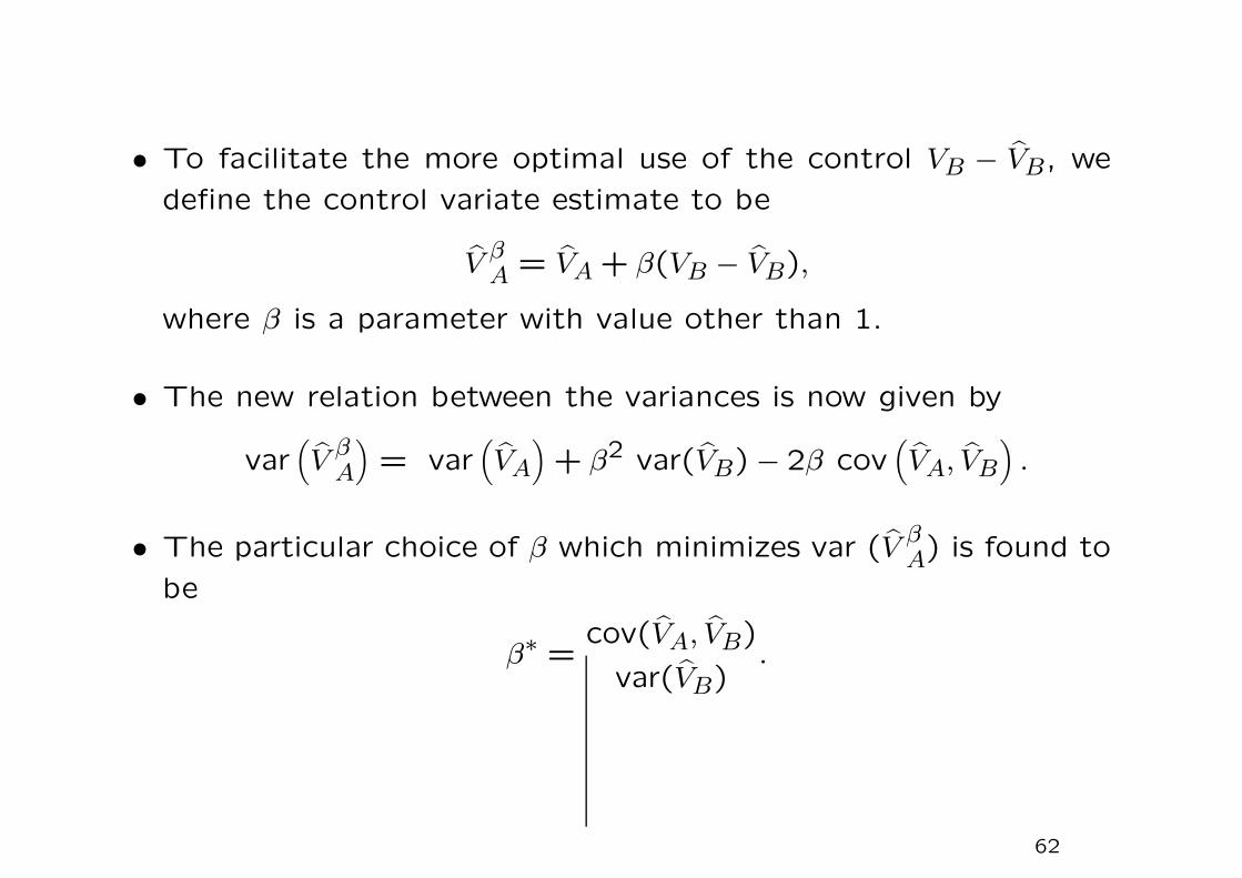
• To facilitate the more optimal use of the control VB − VB, we

define the control variate estimate to be

VβA = VA + β(VB − VB),

where β is a parameter with value other than 1.

• The new relation between the variances is now given by

var(V

βA

)= var

(VA

)+ β2 var(VB) − 2β cov

(VA, VB

).

• The particular choice of β which minimizes var (VβA) is found to

be

β∗ =cov(VA, VB)

var(VB).

62