PRICING CONVERTIBLE BONDS Jonathan A. Batten, Karren Lee

1

PRICING CONVERTIBLE BONDS

Jonathan A. Batten, Karren Lee-Hwei Khaw and Martin R. Young

Jonathan A. Batten Department of Finance Hong Kong University of Science & Technology Clear Water Bay Rd, Sai Kung NT. Hong Kong Email: [email protected] Karren Lee-Hwei Khaw School of Economics and Finance, Massey University Private Bag 11222, Palmerston North, 4442, New Zealand Email: [email protected] Martin R. Young School of Economics and Finance, Massey University Private Bag 11222, Palmerston North, 4442, New Zealand Email: [email protected]

Abstract. Convertible bonds are a developing segment of the corporate bond market.

Nonetheless, the pricing of convertible bonds has not been addressed extensively due to the

complicated optionality and the links between valuation and the underlying risk factors.

Mixed results of mispricing have been reported. Our study clarifies this by a unique sample

that consists of pure convertible bonds to control for complex optionality in these securities

such as the call option. We examine the pricing of the real-time trade prices of the US

convertible bonds. Least squares Monte Carlo simulation approach is used to solve a pricing

model that includes stochastic volatility and credit risk. On average, an underpricing of

6.31% is observed from daily data covering from October 26, 2004 to June 30, 2011.

Stochastic volatility is found to significantly affect the convertible bond pricing. Furthermore,

illiquidity is an important explanatory variable that explain the mispricing of convertible

bonds.

JEL Classification: G13, G15

Keywords: Convertible bonds, pricing, stochastic volatility, real-time trade prices

2

1. Introduction

Convertible bonds are an increasing segment of the corporate hybrid market with

global outstanding market value of US$233 billion, as at 2011. A convertible bond is a

typical example of path-dependent derivative structure that is equivalent to a bond with an

embedded call option on the firm’s stock whereby the fixed-income component acts as a

cushion to the effect of a declining stock price. Convertible arbitrage hedge funds are the

major market players that purchase more than 70% of convertible bonds in the primary

market (Choi, Getmansky, and Tookes, 2009; Mitchell, Pedersen, and Pulvino, 2007). As at

the first quarter of 2008, hedge funds are reported to purchase approximately 80% of the

investments in the privately-placed convertible bonds (Brown, Grundy, Lewis, and

Verwijmeren, 2012).

Pricing models are important tools in setting up investment strategies, including

arbitrage, hedging and asset allocation as well as financing decision such as deciding the

issuance price (Ho and Pfeffer, 1996). Convertible bonds are claimed to sell at discount from

the theoretical values (Ammann, Kind, and Wilde, 2003; Loncarski, ter Horst, and Veld,

2009; Rotaru, 2006). The underpricing is found to remain present over a longer period of

time after the issuance, though it decreases (Loncarski, et al., 2009). Therefore, market

participants specifically the hedge funds actively search for mispricing in convertible bonds

and exploit it usually by buying underpriced convertible bond and taking a short position in

the equity (Ammann, Kind, and Seiz, 2010).

However, existing literature on the pricing of convertible bonds have reported mixed

results from an underpricing of 12.9% (Carayannopoulos, 1996) to an overpricing of

approximately 5% (Barone-Adesi, Bermudez, and Hatgioannides, 2003). In our paper, we

clarify this by a unique sample, consisting of pure convertible bonds that control for complex

optionality in these securities such as the call option. The call feature is valuable to the

issuers but not the investors because it will redistribute wealth between convertible

bondholders and stockholders (Brown, et al., 2012) at any time prior to the maturity, subject

to call provisions such as call protection period, call notice period, and call trigger.

Theoretically, issuers are assumed to call back the convertible bonds when it guarantees

3

conversion but practically issuer do not act optimally1 that leads to biases in the valuation

process (Carayannopoulos and Kalimipalli, 2003). Also, the convertible arbitrage long-and-

hedge strategy becomes complicated with the call feature, thus the hedge funds involvement

in callable convertible bonds is significantly lower (Brown, et al., 2012)2.

Our research fill this gap by highlighting the importance of identifying the option

features present in a convertible bond since it affects the efficiency of a pricing model.

Importantly, former empirical evidence on the convertible bond pricing is generated mainly

from convertibles with complex option features3 such as the call and put. In this paper, we

examine the pricing of real-time trade prices of pure convertible bonds identified from

TRACE-FINRA4 which exclude callable and puttable features. Convertible bonds with

sinking fund, mandatory, exchangeable, reset and reverse clauses are also excluded; so as to

have a sample of pure convertible bonds. To our best knowledge, this is the first study to

examine the pricing efficiency of the convertible bond real-time trade prices. The

dissemination of real-time trade data is meant to increase the transparency level and to enable

the regulators to monitor the market, pricing and execution quality.

We apply the least squared Monte Carlo simulation (LSM) approach (Longstaff and

Schwartz, 2001) to solve for a pricing model that accounts for stochastic volatility and credit

risk. The LSM offers significant gains in computational speed and efficiency in handling

multiple state variables and path dependencies (Longstaff and Schwartz, 2001), thus is

popular among the practitioners (Clément, Lamberton, and Protter, 2002). In the context of

convertible bonds, the empirical evidence on stochastic volatility is still limited. It is

impractical to assume constant volatility for two main reasons. Firstly, the payoff structures

of convertible bonds are contingent on the performance of the underlying stocks. Secondly,

convertible bonds tend to be issued by either unrated or non-investment grade firms (Huang

and Ramírez, 2010), hence are likely to have greater stock volatility. We control for this

1 Refer the recent paper by King and Mauer (2012) for further discussion on the determinants of call policy of convertible bonds. 2 Choi, et. al. (2009) find that the absence of put and call options on a particular stock is associated with greater convertible bond arbitrage activity. 3 For example, 103 callable convertible bonds in King (1986) 30 callable convertible bonds in Carayannopoulos (1996), 1 zero-coupon, callable and puttable convertible bond or LYON in McConnell and Schwartz (1986), 7 callable convertibles in Ho and Pfeffer (Ho and Pfeffer, 1996), 1 callable convertible in Barone-Adesi, et. al. (Barone-Adesi, et al., 2003), 21 callable and puttable convertibles in Ammann, et. al.(2003), 25 callable convertibles in Carayannopoulos and Kalimipalli (2003), 233 callable convertibles in Rotaru (2006) and 32 callable convertibles in Ammann, Kind and Wilde (2008). 4 Financial Industry Regulatory Authority (FINRA) is the largest independent regulator for all securities firms doing business in the US. FINRA disseminates the information through Trade Reporting and Compliance Engine (TRACE) that was officially launched in July 2002.

4

using the constant elasticity of variance (CEV) model. The CEV is considered the simplest

way to extend the Black Scholes model to include the observed inverse dependence of

volatility and the stock price that also associated to the leverage effect (Cox, 1975, 1996). As

for the credit risk, we follow the argument of Tsiveriotis and Fernandes (1998) to keep the

pricing model simple. The fixed-income component of a convertible bond is discounted at a

risk-adjusted interest rate whereas the stock component is discounted at a risk-free interest

rate.

We document an average underpricing of 6.31% from daily observations, estimated

from a sample of 96 pure convertible bonds, covering from October 26, 2004 to June 30,

2011. Consistently, we report underpricing throughout our observation period similar to

Ammann, et. al. (2003), Carayannopoulos (1996), Guschin and Curien (2008), King (1986)

and Rotaru (2006). Equity-like convertible bonds are less underpriced, 0.56%, by the market

than the debt-like convertibles, 10.7%. Excluding the most intense stage of the crisis period

that is during the collapse of Lehman Brothers (September 15, 2008 to March 15, 2009)5, on

average we also document an underpricing of 3.14%. Similarly, the underpricing observed

from the equity-like convertibles is smaller than debt-like convertibles, to be specific 0.27%

and 5.56%, respectively. Equity-like convertibles bonds are less risky and more attractive to

investors because of the higher value of conversion option. On the other hand, debt-like

convertibles are of higher credit risk because the option component is less likely to be

exercised. If the issuing firm is approaching default, the straight bond value of the convertible

could also fall substantially. Furthermore, the pricing of debt-like convertibles are more

challenging than equity-like convertibles. Debt-like convertibles are sensitive to model inputs

and specifications such as the credit spread, default probability and recovery rate.

During the crisis, on average the convertible bonds trade at a deep discount with a

moneyess ratio of 0.543. Therefore, we observe a huge underpricing of 42.97%, in which the

debt-like convertibles are underpriced by 48.271% whereas the equity-like convertibles are

underpriced by 11.122%. During this period, the financial market fell into a period of

extreme volatility with higher probability of default risk. The US Securities and Exchange

Commission (SEC) imposed a temporary ban on short selling6 that adds to the massive

5 We define this period with reference to the 79th annual report of Bank for International Settlements (BIS). 6 SEC bans the short selling for 799 financial companies for three weeks, i.e. from September 19, 2008 to October 2, 2008 as an effort to stabilise these firms and to restore equilibrium to the markets (SEC press release 2008-211, retrieved from http://www.sec.gov/news/press/2008/2008-211.htm).

5

selling pressure from the arbitrageurs. The ban restricted convertible arbitrage opportunities

that cause the arbitrageurs to become liquidity demanders instead of natural liquidity

providers to the market (Choi, Getmansky, Henderson, and Tookes, 2010). Furthermore,

Hedge Fund Research Inc. reported that its convertible arbitrage index realised losses of 34%

in 2008, which is mainly driven by the extreme event from September to November 2008

(Mitchell and Pulvino, 2012).

In addition, we find that stochastic volatility does have a significant effect on the

efficiency of convertible bond pricing. The impact is relatively greater for convertible bonds

with higher underlying stock return volatility. The degree of underpricing decreases

monotonically from 7.34% for the third quintile to 12.26% for the fifth quintile of volatility.

But there are no significant decreases in the underpricing for the first and second quintiles of

volatility. These findings add to the importance of incorporating time-varying effect of

volatility, particularly in the pricing of convertible bonds with substantial fluctuation in

underlying stock returns. Note that the effect of stochastic interest rate is not included in the

subsequent pricing mode. From the preliminary test, we observe insignificant mean

difference in the mispricing between the constant interest rate model and the stochastic

interest rate model. Therefore, interest rate is assumed to be constant, which is consistent

with Ammann, et al. (2008) and Brennan and Schwartz (1980).

In fact, the convertible bond market is relatively illiquid in comparison to equity and

straight bond markets. Therefore, some of the mispricing may be attributable to the illiquidity

of convertible bonds (Ammann, et al., 2003; Loncarski, et al., 2009). In general, illiquidity

may cause significant pricing discrepancies and difficulty to sell an investment or financial

security quickly to meet unexpected cash flow needs. This issue has become increasingly

important to regulators, rating agencies, security exchanges, and institutional investors

(Chordia, Sarkar, and Subrahmanyam, 2005; Longstaff, 1995). To answer this question, we

perform a regression analysis. We find that illiquidity has significant effect on the mispricing

of convertible bonds. Illiquid convertibles tend to be underpriced by the market, as measured

by the convertible bond issuance size and oversubscription of the convertibles at issuance.

Also, riskier convertible bonds, those with longer time to maturity, higher rating code and

greater uncertainty, are more likely to be underpriced. Consistent with Ammann, et al.

(2003), Carayannopoulos (1996), King (1986), Zabolotnyuk, Jones, and Veld (2010), we find

debt-like/out-of-money (OTM) convertible bonds tend to be underpriced whereas equity-

like/in-the-money (ITM) convertible bonds are more likely to be overpriced. Importantly,

6

trades that are executed during the extreme crisis period are significantly underpriced with a

higher degree of mispricing that is consistent with the highly uncertain market condition. This

result also supports our earlier finding of deep underpricing during the collapse of Lehman

Brothers.

The paper is structured as follows. Section 2 reviews the related literature of the

convertible bond pricing models. Section 3 describes the market, data set and the specific

characteristics of the identified convertible bonds, in addition to the valuation framework

including the estimations of parameters and mispricing. Section 3 also describes the testable

predictions that analyse the mispricing of convertible bonds. Section 4 reports and discusses

the results of pricing efficiency. Section 5 concludes.

2. Review of Literature

The theoretical framework for the pricing of contingent claim assets is established

with the well-known publication of Black-Scholes (1973) and Merton’s (1973, 1974) options

pricing model that is further divided into the structural approach (firm-value approach) and

the reduced-form approach (stock-value approach). Ingersoll (1977) views the value of a

convertible bond as a contingent claim on the firm-value. In the initial work, the firm-value is

assumed to consist only of convertible bonds and common stock (Brennan and Schwartz,

1977; Ingersoll, 1977) but is further extended to include senior debt (Brennan and Schwartz,

1980; Nyborg, 1996) and multiple classes of convertible bonds (Lewis, 1991).

The literature on the structural approach of convertible bond pricing is relatively

limited because of its drawbacks. Firstly, the firm-value is neither directly tradable nor

observable in the market, thus it is difficult to estimate the volatility of the underlying asset

(McConnell and Schwartz, 1986; Nyborg, 1996). Secondly, the solution to the partial

differential equation (PDE) of the contingent-claim becomes complicated when the model

considers more complex capital structure (Takahashi, Kobayashi, and Nakagawa, 2001;

Zabolotnyuk, et al., 2010). Consequently, the reduced-form approach is introduced by

McConnell and Schwartz (1986) to price convertible bonds that view the security as a

contingent claim of the underlying common stock.

Either a closed-form or a numerical solution can be applied to solve the value of

convertible bonds, depending on the underlying assumptions governing each pricing model.

7

Closed-form solution is restricted to perfect market assumptions and continuous time factor

so it is unlikely to generalise the solution (Ingersoll, 1977; Lewis, 1991) Market

imperfections, path-dependent payoff structures and boundary conditions could not be

integrated in the pricing model (Nyborg, 1996; Wilde and Kind, 2005). Therefore, numerical

solutions such as the (1) finite difference method (Ayache, Forsyth, and Vetzal, 2003;

Brennan and Schwartz, 1977, 1980; Takahashi, et al., 2001; Tsiveriotis and Fernandes, 1998;

Yigitbasioglu, 2002), (2) finite element method, (3) tree model (Chambers and Lu, 2007;

Hung and Wang, 2002; Yagi and Sawaki, 2010) and (4) simulation model (Lvov,

Yigitbasioglu, and El Bachir, 2004; Wilde and Kind, 2005) are suggested.

A simulation method is usually recommended in solving the valuation of high-

dimensional derivative securities because the convergence rate is independent of the number

of state variables (Fu, Laprise, Madan, Su, and Wu, 2001; Ibáñez and Zapatero, 2004).

Though, both finite difference and lattice-based methods are appropriate in solving early

exercise features, these methods are still lacking in terms of the speed of computation. These

methods are efficient to solve for pricing models with one or two sources of uncertainty

(Broadie and Glasserman, 1997; Longstaff and Schwartz, 2001) because the convergence rate

is exponential in the number of state variables. As a result, simulation is claimed to be

increasingly attractive in handling multiple state variables and path dependencies (Broadie

and Glasserman, 1997; Ibáñez and Zapatero, 2004; Longstaff and Schwartz, 2001).

Brennan and Schwartz (1980) allow for two stochastic state variables, particularly the

firm-value and interest rate. But the differences generated by the one-factor model and the

two-factor model are relatively small. Therefore, Brennan and Schwartz (1980) conclude that

it is more computational efficient to assume a flat term structure. Amman, et. al. (2008) and

Carayannopoulos (1996) support the claim but Barone-Adesi, et. al. (2003) and Ho and

Pfeffer (1996) claim otherwise. Credit risk has been an important consideration in the pricing

model. In the structural approach, the possibility of bankruptcy is determined endogenously.

A company would fall into bankruptcy when the total firm-value (Brennan and Schwartz,

1977; Ingersoll, 1977; Lewis, 1991) or the net total firm value7 (Brennan and Schwartz, 1980;

Nyborg, 1996) falls below the total redemption value of the convertible bonds. On the

contrary, the reduced-form approach precludes the possibility of bankruptcy, thus

overestimating the value of convertible bonds. In the reduced-form approach, credit risk has

7 Net total firm value equals to the total firm value minus total senior debt.

8

to be estimated exogenously. For example, McConnell and Schwartz (1986) add a constant

credit spread to the risk-free rate to capture the credit risk.

Tsiveriotis and Fernandes (1998) refute the credit risk claim of McConnell and

Schwartz (1986), claiming that a convertible bond can be decomposed into two components.

The fixed income component of a convertible bond8 is exposed to credit risk, whereas the

stock component has zero default risk because the issuer can always deliver its own stock.

For these reasons, the fixed income component is discounted at a risk-adjusted rate and the

stock component is discounted at the risk-free rate. Then, the credit risk consideration is

extended to include the probability of default, hazard rate, fractional loss as well as recovery

upon bankruptcy (Ayache, et al., 2003; Takahashi, et al., 2001). In practice, there is limited

market credit information when pricing convertible bonds, particularly in modelling the

hazard rate and the fractional loss, which are not observable. As a result, practitioners are

more likely to use the Tsiveriotis and Fernandes (1998)’s model in setting up investment and

hedging strategies because this model only requires the estimation of credit spreads.

As for the equity risk, conventionally, the underlying asset of a convertible bond is

assumed to follow a lognormal distribution with constant volatility, which is impractical

when the payoff structure is dependent on the stock price. Moreover, the life of a convertible

bond is typically longer, thus the variance of stock return may change substantially.

Practitioners also recognise the drawback of assuming constant volatility. Therefore, they

have to constantly adjust the variance rate estimated in the model (Macbeth and Merville,

1980). In brief, the subject of stochastic volatility in convertible bond pricing has not been

studied extensively. For example, the implied volatility (Barone-Adesi, et al., 2003), local

volatility (Yigitbasioglu, 2002), multiple levels of historical volatility (Lvov, et al., 2004), the

CEV model (Das and Sundaram, 2007), and the GARCH model (Ammann, et al., 2008).

Empirically, the results are found to be mixed. An average underpricing between

1.94% (Landskroner and Raviv, 2008) and 12.9% (Carayannopoulos, 1996) to an average

overpricing between 0.36% (Ammann, et al., 2008) and approximately 5% (Barone-Adesi, et

al., 2003) have been reported. Out-of-money (OTM) convertible bonds tend to be

underpriced whereas in-the-money (ITM) convertible bonds are more likely to be overpriced

(Ammann, et al., 2003; Carayannopoulos, 1996; King, 1986; Zabolotnyuk, et al., 2010). But

8 The fixed-income component includes of periodic coupon payments, final redemption payment and any call or put provisions which are dependent on the issuer’s timely access to the required cash amount.

9

interestingly, Ammann, et. al. (2008) and Landskroner and Raviv (2008) find evidence of

underpricing in the ITM convertible bonds. The relation between the mispricing and term to

maturity is also found to be inconsistent. King (1986) claims that convertible bonds with

shorter term to maturity are more likely to be underpriced by the market but Ammann, et. al.

(2003) and Landskroner and Raviv (2008) claim otherwise. The value of a convertible bond

is also sensitive to the underlying assumption of dividend yield/payment (Ammann, et al.,

2008; McConnell and Schwartz, 1986), coupon payment (Ammann, et al., 2008; Lau and

Kwok, 2004; Rotaru, 2006), and the conversion ratio (Lau and Kwok, 2004; Rotaru, 2006).

In addition to the model-related risk factors (interest rate risk, equity risk, and credit

risk) and the issue-specific factors (moneyness, maturity, coupon, conversion ratio, and

dividend), boundary conditions, in particular the call provisions, do affect the pricing of

convertible bonds. Theoretically, issuers are assumed to act optimally by calling the

convertible bonds when it guarantees conversion. But in practice the convertible bonds are

not called immediately even though the conversion price equals the call price because of the

prespecified call restrictions that leads to estimation biases. Existing empirical studies have

been focusing on examining the pricing of convertible bonds with complex option features,

such as the call and put. For example, 21 callable and puttable convertibles in Ammann, et.

al.(2003), 25 callable convertibles in Carayannopoulos and Kalimipalli (2003), 233 callable

convertibles in Rotaru (2006) and 32 callable convertibles in Ammann, Kind and Wilde

(2008).

In brief, reported inconsistencies are generally attributable to the limitations and

differences of the model specifications. There are also concerns with the length of the study,

or the statistical limitations due to few observations and relatively small sample size. These

limitations may generate estimation biases and limit the ability to generalise the results and

models used. In a nutshell, there remains scope for further examination of the question of

convertible bond valuation.

3. Data and Methodology

3.1 Market

This study examines the US convertible bond market for two main reasons. Firstly,

the US market has the largest convertible bond market, evidenced by the highest market share

10

followed by Europe, Japan and Asia-Pacific (refer Table 1). Throughout the observed period

(year 2000 to 2011), US holds more than half of the convertible bond market share, with the

highest market share of 73.25% in 2007. In 2011, the market share has slightly decreased to

63.64%. Secondly, the real-time trade data of convertible bonds are disseminated by the

Financial Industry Regulatory Authority (FINRA), the largest non-governmental regulator for

all securities firms doing business with the US public. In July 2002, FINRA officially

launched Trade Reporting and Compliance Engine (TRACE) to disseminate over-the-

counter9 (OTC) corporate bond real-time trade data and trade volume information to the

public. For the investors, the real-time trade data are meant to better gauge the quality of the

execution they are receiving from their broker-dealers. The dissemination of the information

not only increases the levels of transparency but is also intended to enable the regulators to

monitor the market, pricing and execution quality.

(INSERT TABLE 1 ABOUT HERE)


TRACE was implemented in three phases (refer Table 2). Phase I was implemented

on July 1, 2002 to disseminate the trade information for (1) investment grade securities with

an initial issue size of US$1 billion or greater and (2) 50 non-investment grade (high yield)

securities disseminated under FIPS210 that are transferred to TRACE. Thus, by the end of

2002, FINRA disseminated the transaction information for approximately 520 securities.

Subsequently, phase II was implemented on April 14, 2003 to further disseminate (1) all

investment grade securities of at least US$100 million par value (original issue size) or

greater rated A3/A- or higher, (2) a group of 120 investment grade securities rated Baa/BBB,

and (3) 50 non-investment grade bonds. In total, the number of disseminated bonds increased

to approximately 4,650 bonds. Eventually, it was fully phased in by January 2006, offering

real-time, public dissemination of transaction and price data for all publicly traded corporate

bond, including convertible bonds. Nonetheless, any transactions pursuant to Rule 144A11 are

not disseminated.

9National Association of Securities Dealers, NASD (2004) estimates that 99% of the US corporate bond trading is transacted over-the-counter. 10Before the launching of TRACE, the dissemination of real-time trade data for high yield bonds was collected by NASD under the Fixed Income Pricing System (FIPS). 11 Rule 144A, adopted by the Security and Exchange Commission of US (SEC) came into effect on April 30, 1990 to provide a safe harbour exemption from the registration requirements of the Securities Act (1933) for resale of restricted securities among ‘qualified institutional buyers’(QIBs) ( http://www.sec.gov/)..

11

3.2 Sample Selection

This study examines the pricing of real-time trade data of the US convertible bonds that are

disseminated by TRACE of FINRA (TRACE-FINRA). Initially, we identified 511

convertible bonds that are offered before June 30, 2011. June 30, 2011 is selected as the end

date for the study because at that time, the US government temporarily stopped issuing 5- and

7- year bonds (refer Figure 1). The mean maturity of our sample is 5.927 years (refer Table

3), which is between the US government 5- and 7- year bonds. When the issuance of the US

government bonds recommenced, the bonds’ credit rating had reduced. Therefore, including

convertible bonds after June 30, 2011 could cause bias.

(INSERT FIGURE 1 ABOUT HERE)

301 convertible bonds are found to be attached with callable feature. These

convertible bonds have to be excluded from our sample selection to control for the impact of

non-optimal call on pricing efficiency12, thus reducing the sample to 211 convertible bonds.

The sample also excludes convertible bonds that are attached with puttable, sinking fund or

mandatory13 features. In addition, our selection criteria require the convertible bonds to be

public bonds issued by the US local firms, to have prospectus in EDGAR14 and with active

underlying common stock of the issuer. Therefore, exchangeable convertible bonds15 and

convertible bonds with delisted underlying stock or have filed for Chapter 11 are also

excluded to ensure our sample consists only of pure convertible bonds. These criteria further

reduce the sample size to 177 convertible bonds.

Furthermore, the sample requires the convertible bonds to have credit ratings to

account for credit risk. Only 33 convertible bonds are found to be rated. In view of that, we

12 The valuation process also becomes very complicated if all the features of convertible bonds are taken into consideration (Lau and Kwok, 2004). Nonetheless, the pricing model can be extended to incorporate these features into the valuation of convertible bonds in the future study. 13 A mandatory convertible bond is a bond that has to be converted mandatorily into equity at maturity. 14 EDGAR, the Electronic Data Gathering, Analysis, and Retrieval system, performs automated collection, validation, indexing, acceptance, and forwarding of submissions by companies and others who are required by law to file forms with the U.S. Securities and Exchange Commission (SEC). Its primary purpose is to increase the efficiency and fairness of the securities market for the benefit of investors, corporations, and the economy by accelerating the receipt, acceptance, dissemination, and analysis of time-sensitive corporate information filed with the agency. 15 An exchangeable bond has approximately the same features as the conventional convertible bond but the payoff of an exchangeable bond depends on the underlying stock of another company. In brief, the bondholder is granted an option to exchange the bond for shares of another company.

12

take the credit rating of the issuer when the convertible bond is not rated, which is consistent

with existing studies (Ammann, et al., 2008; Rotaru, 2006). Rating information for the

convertible bonds is also disseminated by TRACE-FINRA whereas rating information for the

issuer is obtained from Moody’s. After imposing these selection criteria, we have a unique

sample consisting of 96 issues of pure convertible bonds. A pure convertible bond is defined

as a bond embedded with only the conversion provision.

The observation period covers from the first trade date disseminated by TRACE-

FINRA for the selected sample, i.e., from October 26, 2004 through June 30, 2011. This

study examines the pricing efficiency on daily observation, thus we have to calculate the

intraday average price from the disseminated real-time data. Trades that are cancelled are

excluded to avoid repetition in the data. From the beginning of November 2008, TRACE-

FINRA identifies the reporting party for each real-time data. TRACE-FINRA disseminates

three reporting party indicators – B, S and D for the real-time data. B and S represent the

customer trade whereas D represents the inter-dealer trade which is always a sell. B is where

reporting party (dealer) bought from a customer and S is where reporting party (dealer) sold

to a customer.

We have four types of real-time intraday average price for comparison, with the total

number of daily observations in the parentheses for the whole sample, i.e. the MPAll

(41,774), MPBuyer (26,756), MPSeller (24,720), and MPDealer (19,634). MPAll represents

the daily intraday average trade prices from October 26, 2004 through June 30, 2011 without

distinguishing the reporting parties. But from November 2008 onwards, we have MPBuyer,

and MPSeller to represent the retail trade prices and MPDealer that represent the wholesale

trade prices.The convertible bond specific data such as the maturity at issuance, coupon rate,

conversion price, conversion premium at offering, amount of issuance and credit rating are

collected from TRACE-FINRA and Thomson Reuters EIKON. Any inconsistent data found

between TRACE-FINRA and EIKON is verified against the issuers’ prospectus or official

filings to the US Securities and Exchange Commission (SEC) that are publicly accessible via

EDGAR. On the other hand, the corresponding synchronous stock prices are collected from

Datastream.

13

3.3 Sample Descriptions

Table 3 reports the summary statistics for the overall sample of 96 convertible bonds. The

mean maturity at issuance is 5.927 years with the longest maturity of 20 years. Average

coupon rate is at 3.75%. The range for the coupon rate is wide – from as low as 0.375% to a

high rate of 15%. On average, the convertible bond can be converted at a conversion price of

US$32.105 per share and a conversion premium at offering of 31.059%. Conversion

premium measures the excess of the conversion price over the stock price at issuance as a

percentage of the stock price

. A relatively low conversion

premium indicates a more equity-like convertible bond and vice-versa (Brown, et al., 2012).

The mean total issuance is approximately US$425 million with an average overallotment of

US$16 million. On average, the Moody’s rating is between Ba2 and Ba3. According to the

rating definition, securities rated Ba are judged to have speculative elements and are subject

to substantial credit risk.


This is of no surprise because access to the convertible bond market is more flexible

for issuers who have difficulty entering the traditional bond market due to restrictive rating

requirements. A good example is the growth firm. A growth firm is reluctant to issue a

significant amount of straight bond because the higher fixed income obligation tends to

increase the expected cost of financial distress of a firm. Besides, a growth firm does not

favour issuing common stock if the current stock price does not reflect the firm’s growth

opportunities. So, the issuance of equity is expected to cause excessive dilution on existing

stockholders’ claims (Chang, Chen, and Liu, 2004; Stein, 1992).

To provide some in-depth description, we subsample the convertible bonds by the

observed conversion provision and the type of placement when the securities are first issued.

Summary statistics of the subsamples are discussed in turn. From the sample, 34 convertible

bonds (subsample 1) are identified to be issued without any conversion restriction, in which

the convertible bonds can be converted at any time prior to the maturity. Conversely, 62

convertible bonds (subsample 2) are attached with conversion restrictions. The restrictions

are identified from the issuer’s prospectus, stating that the conversion option can only be

exercised within the prespecified conversion timeframe, the conversion is only allowed if the

prevailing stock price exceeds the conversion price for at least a certain percentage (for

example, more than 130% of the conversion price per share) and for a certain period of time

14

(for example, at least 20 trading days in a period of 30 consecutive trading days). These

provisions restrict the bondholders from immediate conversion though the prevailing stock

price exceeds the conversion price.


Panels A and B of Table 4 describes the summary statistics for subsamples 1 and 2,

respectively. Then, Panel C reports the test of mean differences for the observed

characteristics. Statistical evidence claims that there are significant differences at 1% level, in

the coupon rate and conversion price between the two subsamples. Subsample 1 is issued at a

higher coupon rate, with a mean of 4.86% and a wider range from 1.25% and 15%, but

subsample 2 is issued at a lower coupon rate, with a mean of 3.141% and a range from

0.375% to 6.5%. This finding possibly explains the reason for issuing convertible bonds with

conditional conversion. Lower coupon rates expose the issuers (in subsample 2) to relatively

lower fixed-income obligation, thus the conversion restrictions enable the issuers to take

advantage of the lower interest rate environment. The mean conversion price for subsample 2

is significantly lower than subsample 1 at 1% level by US$13.113 per share but no statistical

difference is found for the conversion premium at offering. As for the other observed

characteristics the mean differences are found to be statistically insignificant.

Next, we discuss the characteristics of the sample, grouped by the type of placement

when the convertible bonds are first issued. The type of placement can be identified from

Datastream and is confirmed against the issuer’s prospectus in EDGAR. Equally, there are 48

convertible bonds in each subsample. Subsample A includes of convertible bonds that are

first issued via private placement pursuant to Rule 144A that are subsequently registered with

the US Securities and Exchange Commission (SEC) to be public issues16 whereas subsample

B consists of convertible bonds that are issued via public placement. Existing studies (Fenn,

2000; Huang and Ramírez, 2010; Livingston and Zhou, 2002) have reported tremendous

increase in the size of 144A debt market, ever since the rule came into effect on April 30,

1990. Specifically, Huang and Ramírez (2010) document that the total offering of convertible

bonds in the 144A market increased from US$1.4 billion in 1991 to US$22.4 billion in 2004.

16 Huang and Ramírez (2010) found that approximately 88% of the convertible debts and 91% of the straight debts issued via Rule 144A are subsequently registered with the SEC. For over 80% of these issues, the registration is found to be filed within three months of issuance but Fenn (2000) found a longer period, ranging from three to seven months for high-yield bonds. Huang and Ramírez (2010) further claim the difference is because they use the date of registration with SEC instead of the time of completion of the exchange offer used to complete the registration.

15

On contrary, the total offering via the public placement decreased from US$9.7 billion in

1991 to US$4.8 billion in 2004.

Below-investment grade issuers are claimed to be more likely to issue bonds via the

144A market with options to register the securities with the SEC (Fenn, 2000). The 144A

market provides a leeway for the low credit rating firms to issue securities quickly in order to

meet their urgent financing needs because the disclosure requirements are less stringent

(Fenn, 2000; Huang and Ramírez, 2010; Livingston and Zhou, 2002). Therefore, the speed

of issuance hypothesis significantly explains the growth of the 144A market (Fenn, 2000;

Huang and Ramírez, 2010). In addition, Huang and Ramírez (2010) find that QIBs17 have

advantages over public lenders in dealing with firms with high credit risk and information

asymmetry, supporting the lender specialisation hypothesis.


Panels A and B of Table 5 describe the summary statistics for subsample A and

subsample B, respectively whereas Panel C reports the test of mean differences of the

observed characteristics. Credit rating is found to be insignificant, possibly because of the

nature of the available data used in our study, which may affect the convertible bonds in

subsample A. The ratings are the bonds’ rating when they have become public issues.

Furthermore, issuers in the 144A market have the options to get credit ratings for their

securities between the offering and the subsequent registration dates for two main reasons.

Firstly, the QIBs are less dependent on credit ratings than the public investors and secondly

the application for credit ratings would delay the issuance process of 144A securities (Huang

and Ramírez, 2010).

Statistically, the convertible bonds in subsample A are issued with longer maturity at

issuance with a mean difference of 0.729 years, significant at 10% level, similar to Huang

and Ramírez (2010)18. Conversely, the mean coupon rate for subsample A is significantly

lower than subsample B, at 1% level, with a mean difference of 1.166%. Rule 144A is meant

17QIBs are defined as institutions that own or have investment discretion over $100 million or more in assets. In addition to the $100 million requirement, banks and savings and loan associations must also have at least $25 million of net worth to qualify as QIBs. For registered broker-dealers, $10 million investment in securities would meet the requirement (Livingston and Zhou, 2002).Hedge funds are found to be one of the major group of QIBs, in which 73.4% of the financing of newly-issued convertibles is provided by hedge funds (Brown, et al., 2012). 18 Huang and Ramírez (2010) reports a higher mean maturity at issuance of 12.74 years for 554 convertible bonds that were first issued via Rule 144A and 9.68 years for 188 convertible bonds that were issued via non-shelf public placement.

16

to encourage speedy issuance because debt issuers are not required to file pre-issued

registration with the SEC. Therefore, timely issuance enables the firms to take advantage of

favourable market conditions, such as lower interest rates (Huang and Ramírez, 2010). The

mean conversion price for subsample A is significantly higher than subsample B at 5% level

by US$10.891 per share. Nonetheless, there is no statistical difference in mean, found for the

conversion premium at offering.

In addition, the total issuance for subsample A is significantly higher with a mean

difference of US$177.263 million, at 5% level but significantly lower amount of

overallotment at 1% level. The mean difference of the subsamples for overallotment is

US$30.475 million. In general, debt issued via Rule 144A have smaller base of potential

buyers (only the QIBs), less stringent disclosure requirements and weaker legal protection.

Because of these, the 144A debt are claimed to be less liquid and have considerable risk, thus

producing yield premium over public issues (Fenn, 2000; Livingston and Zhou, 2002). As a

result, issuers in the 144A market are more likely to issue larger bond size because investors

are more likely to ask for lower rate of return for larger issues that are usually more liquid

than small issues (Fenn, 2000; Livingston and Zhou, 2002)19. Furthermore, there is evidence

of negative relation between gross underwriter spread and size of issuance, explained by the

economies of scale (Livingston and Zhou, 2002). For subsequent test, we only provide

subsamples by the terms of conversion because rationally, once these convertible bonds are

registered to become public issues, type of placement is assumed not to have significant on

the pricing efficiency.



Next, Table 6 reports the characteristics of the real-time trade prices disseminated by

TRACE-FINRA and the moneyness of the convertible bonds. The daily trade price is

calculated by taking the average of the real-time intraday price, which is reported at US$100

when trading at par, though the actual face value of each convertible bond is US$1,000.

Averaging from October 26, 2004 through June 30, 2011, the daily real-time trade price

(MPAll) is US$110.972. Retail trades denoted by MPBuyer and MPSeller are recorded at

19 Huang and Ramírez (2010) also reports a higher mean gross proceeds US$259 million for 554 convertible bonds that were first issued via Rule 144A and US$182 million for 188 convertible bonds that were issued via non-shelf public placement.

17

US$112.035 and US$111.824, respectively, whereas the wholesale trade denoted by

MPDealer is recorded at US$110.031. The moneyness20 is calculated by taking the ratio of

the prevailing underlying stock price over the prespecified conversion price. The mean

moneyness is 0.84, and with reference to Mitchell and Pulvino (2012)21 we define convertible

bonds with moneyness less than 0.84 as debt-like (credit-sensitive), whereas convertible

bonds with moneyness greater than 0.84 as equity-like (equity-sensitive). Table 7 reports

statistically insignificant mean difference between the retail trade prices. But the retail trade

prices are found to be significantly higher than the wholesale trade prices, at 1% level

probably due to lower trade frequency.


We also report the market data by terms of conversion. From Panel C of Table 8,

convertible bonds that are issued without conditional conversion are priced significantly

higher than the convertible bonds that are issued with conditional conversion, at 1% level and

the results are consistent for all types of trade prices. On average, subsample 1 consists of

equity-like convertible bonds, whereby subsample 2 consists of debt-like convertible bonds

with moneyness ratios of 0.974 and 0.797, respectively. Convertible bonds in subsample 1

offer better flexibility to the bondholders than subsample 2 because the bondholders are not

restricted to convert the convertible bonds at any time prior to maturity whenever the

condition guarantees conversion. Therefore, rationally bondholders are more likely to pay

higher value for non-conditional convertibles22 as compared to those in subsample 2 that limit

the bondholders from taking immediate advantage of the favourable market condition.

We examine the characteristics of real-time trade prices, and moneyness by

subperiods for two reasons. First of all, the observed market data are time varying and

secondly, our observation period includes the extreme period of financial instability. The

subperiods are defined with reference to the 79th annual report of Bank for International

20 To be consistent with literature on convertible bond pricing, we choose to report the moneyness instead of conversion premium. 21 Mitchell and Pulvino (2012) sort their sample by the median of moneyness. Similarly, we sort our sample by the median of moneyness (0.77) and we find the results for the subsequent tests are indifferent whether the sample is sorted by the mean or median of moneyness. 22 The justification is related to the value between non-callable and callable convertible bonds. The value of a plain vanilla convertible bond is higher than the value of a callable convertible bond but the difference decreases as the default risk increases (Das and Sundaram, 2007). An investor is more likely to pay higher value for a callable convertible bond with better call protection such as more stringent hard call and/or soft call provisions that makes it more difficult for the issuer to initiate a call (Gong and Meng, 2007; Lau and Kwok, 2004).

18

Settlements (BIS)23, but with slight changes to fit our sample periods. We define six

subperiods for our sample. Subperiod 1 starts prior to the subprime-mortgage-related turmoil

(prior to mid-August 2007); Subperiod 2 covers the subprime-mortgage-related turmoil (from

mid-August 2007 to mid-September 2008); Subperiod 3 includes the most intense stage of

the crisis (from the collapse of Lehman Brothers, i.e. September 15, 2008 to mid-March

2009); Subperiods 4, 5 and 6 are the recovery stages. The recovery stage is further divided

into three subperiods with the intention of examining the gradual recovery, i.e., from mid-

March 2009 to December 2009, 2010, and the first six month of 2011.



Panel A of Table 9 summarises the statistics of the sample, whereas Panels B and C

are for the subsamples by conversion terms. Table 9 only reports the real-time trade price

measured by MPAll because it provides an inclusive observation for the identified

subperiods, including the pre and post crisis periods. MPAll and moneyness shows a

statistically significant decreasing trend from Subperiod 1 to Subperiod 3 and a gradual

increasing trend from Subperiod 4 to Subperiod 6, at 1% level (refer Table 10). Statistically,

greater significant mean differences are found when every subperiod is compared against the

most intense period (Subperiod 3). During the extreme crisis period, the US Federal Reserve

responded by lowering interest rates, whereas the US Securities and Exchange Commission

(SEC) imposed temporary ban on short selling within a week of Lehman’s collapse. The ban

restricted convertible arbitrage opportunities that causes the arbitrageurs to become liquidity

demanders instead of natural liquidity providers to the market (Choi, et al., 2010).

Furthermore, Hedge Fund Research Inc. reports that its convertible arbitrage index realised

losses of 34% in 2008, which is mainly driven by the extreme event from September to

November (Mitchell and Pulvino, 2012)

Prior to the subprime-mortgage-related turmoil (Subperiod 1), on average the

convertible bonds are equity-like, traded at US$112.119 that decreases to US$108.483 in

Subperiod 2. The moneyness decrease to 0.543 during the collapse of Lehman Brothers

23 BIS defines five stages of the global financial crisis, i.e. Stage 1 – Pre-march 2008: Prelude to the crisis, Stage 2 – Mid-March to mid-September 2008: Towards the Lehman bankruptcy, Stage 3 – 15 September 2008 to late October 2008: Global loss of confidence, Stage 4 – Late October 2008 to mid-March 2009: Global downturn and Stage 5 – Since mid-March 2009: Downturn deepens but loses speed ("79th Annual Report 1 April 2008 - 31 March 2009," 2009).

19

(Subperiod 3), traded at US$77.56. The relatively low moneyness confirms the debt-like

feature of the convertible bonds. Thereafter, the MPAll increases to US$101.393 in the last

three quarters of 2009, then to US$117.255 in 2010, and to US$130.162 in the first half of

2011. On average, the moneyness improves to 0.717, 0.863 and 0.997, respectively. The

increase signifies a gradual change from debt-like to equity-like convertible bonds. Similar

trends are observed in the subsamples.

Next, we examine the impact on the trade prices following the changes in the

moneyness. Moneyness is measured as the ratio of stock price over conversion price. Since

the conversion price stays relatively constant throughout the life of a convertible bond24, the

major driver of a change in the moneyness is the performance of the stock price that affects

the value of a convertible bond. MPAll and moneyness are found to be positively related

though moneyness is indifferent between Subperiods 1 and 2 (refer Table 11). Moving from

Subperiods 2 to 3, MPAll decreases by US$0.07525 when moneyness decreases by one basis

point. Once the market starts to pick up in Subperiod 4, consistently MPAll increases by

US$0.074 for every one basis point increase in the moneyness. The momentum increases to

US$0.077, from Subperiods 4 to 5 and to US$0.083, from Subperiods 5 to 6 for every one

basis point increase in the moneyness.

3.4 Valuation Framework

This study employs Longstaff and Schwartz’s (2001) stock-based least squares Monte Carlo

simulation model (LSM) for the pricing of convertible bonds. LSM is selected because

convertible bonds are subject to multiple sources of risk and path-dependent features. LSM

provides a path-dependent approximation using information contained in a sample of

simulated paths by means of simple regression. Following Longstaff and Schwartz (2001),

this study assumes a finite time horizon [0, T], where t = 0 indicates today and t = T indicates

the day of maturity for a convertible bond.

The probability space is defined as (Ω, F, P) and an equivalent martingale measure Q

subject to assumption of no arbitrage opportunities. Ω is the set of all possible outcomes ω of

the state variables for pricing convertible bonds between time 0 to T, F is the sigma field of

24 But the conversion price (conversion ratio) is typically adjusted for stock split and stock dividends. 25 The change in MPAll is calculated on the actual face value, US$1,000 of each convertible bond to provide a clear relation between the trade price and moneyness.

20

distinguishable events at time T, and P is the probability measure corresponding to F. Let

, ; , , ∈ Ω, ∈ , denote the payoff of a convertible bond, conditional on the

convertible bond is being exercised after t and both the issuer and investor follow optimal

exercise strategies for all stopping time s.

The point in time whereby the embedded option is executed, leading to premature

exercise is termed as optimal stopping time ∗. The convertible bond is terminated

immediately and the bondholder is not entitled for any coupon payments and redemption

value after ∗. The total payoff for a convertible bond is different from an option. At ∗ the

bondholder will also get the periodic coupon payments accumulated from the existence of the

bond until τ* together with the payoff illustrated in Table 11. Some convertible bonds also

contain accrued interest payments. As a result, the total payoff , ∗; , from a

convertible bond at ∗equals to

, ∗; , , ∗, , ∗ (1)

where , ∗; , is the optimal payoff from the convertible bond subject to boundary

conditions, at ∗ and ∗ is the present value at ∗of all coupon and accrued interest

payments arising during the period , ∗ . Once the optimal exercise decisions and

corresponding payoffs are determined for each path, the value of convertible at is

calculated by averaging the discounted payoff over all the simulated paths.

∑

∗

,, ∗; , (2)

where ∗ are the optimal stopping times for each path i, . are the corresponding total

payoffs, and , is the instantaneous risk-free interest rate during the period , ∗ in

path i.


The valuation process considers discrete time, with daily frequency and time t

belonging to a set of finite number of stopping times … with 0 and

. Table 11 summarises the payoff , ; , of a convertible bond when the state

21

path ω is realised, at time s. At maturity, the payoff , ; , is equal to the

maximum of conversion value or redemption value where is the conversion ratio,

is the underlying stock price at maturity, and is the face value of the convertible bond.

At each exercise time point , prior to maturity, subject to certain prespecified time

restrictions (if there is any), the convertible bondholders have the right to either convert the

convertible bonds into shares of common stock or continue holding the bond and revisit the

exercise decision at the next exercise time. The convertible bondholders have to compare the

payoff for immediate exercise, in this case the conversion value with the expected payoff for

continuation or the continuation value ; . The conversion value is known at but not

the continuation value. Continuation value is the value of holding the convertible bond for

another period instead of exercising immediately. It is not observable, thus has to be

estimated.

Assuming no arbitrage opportunity, the continuation value ; can be expressed

as the expectation of the remaining discounted cash flows , ; , with respect to the

risk-neutral pricing measure Q. Specifically, at time the continuation value is given as

; ∑,

, ; , Ƒ (3)

where , is the riskless discount rate, and the expectation is taken conditional on the

information set Ƒ at time (Longstaff and Schwartz, 2001).

A convertible bondholder opts for conversion before maturity when the conversion

value is greater than the continuation value ; in order to maximise the payoff

of a convertible bond. Otherwise, if the continuation value ; is greater than the

conversion value at time , a rational investor would continue holding the convertible

bond and revisit the exercise decision at the next exercise time .

3.5 Parameter Estimation

3.5.1 Stock Dynamic

22

The payoff structure of a convertible bond is dependent on the performance of the underlying

stock price. Conventionally, under the perfect market assumptions, the Black-Scholes model

assumes that the underlying stock price follows the geometric Brownian motion

0 (4)

where is the stock price at time , is the change in over the period , , µ is

the drift rate, σ is the volatility of the instantaneous return on , and is the Brownian

motion with an initial condition 0. Both µ and σ are constant and are independent of

time and the current stock price.

The volatility is measured by standard deviation, estimated on historical basis, using

the time series data of the underlying stock.

N

tt RR

Nˆ

1

2

1

1 (5)

Historical standard deviation is model free (Poon and Granger, 2005), thus easy to calculate

and requires no prior assumption about the stock market efficiency (Rotaru, 2006), but the

major concern is the choice of how much past data to include and the frequency of the data

(Green and Figlewski, 1999; Poon and Granger, 2005). Since our study examines the pricing

on daily basis, it is consistent to employ daily data in each of the parameters. As for the daily

data, only trading days will be considered because volatility is found to be larger when the

exchange is open (Fama, 1965) and volatility is claimed to be affected by trading (French and

Roll, 1986). Therefore, the volatility for each convertible bond is calculated using daily

individual stock returns of 252 trading days prior to the first real-time trade data reported to

TRACE-FINRA and is assumed to be constant.

A number of stylised facts on volatility have emerged over the years such as thick

tails, volatility clustering, volatility smiles and skews, long memory and persistence, leverage

effects, and volatility co-movements. Thus, it is unrealistic to assume constant volatility,

specifically in our study since our observation period includes the global financial crisis

(2007 to 2009) that causes great fluctuations in the financial markets. Therefore, the constant

elasticity of variance (CEV) model is applied to control for the effect of volatile equity

market. The CEV model is often considered to be the simplest way to extend the Black

Scholes model to include the observed inverse dependence of volatility and the stock price a

23

foundation for the observed implied volatility skew that is also associated to the leverage

effect (Christie, 1982; Cox, 1975, 1996).

The CEV model assumes that stock price, takes the following form.

0, 2 (6)

where is the stock price at time , is the change in over the period , , µ is

the expected growth rate of , σ is the volatility of the instantaneous return on , and is

the Brownian motion with an initial condition 0. Both µ and σ are constant and are

independent of time and the current stock price. Conventionally, the CEV model retains the

constant volatility assumption of the Black Scholes model, but it introduces an additional

parameter to denote the elasticity, β of the instantaneous volatility of the stock return. The

level of elasticity will determine the dynamics of the underlying stock price. In Cox’s (1975,

1996) study, the elasticity is bounded to 0 ≤ β < 2. When β = 2, the CEV model is identical

to the Black-Scholes model, thus the variance rate is independent of the stock price. For this

reason, the Black-Scholes model is claimed to be affiliated to the CEV model. When the

elasticity decreases, the process becomes less volatile, and the reverse when the elasticity

increases. This adjustment causes the absolute level of variance to decline (rise) as the stock

price rises (declines), thus integrating an inverse relationship between stock prices and

volatility; a phenomenon referred as the leverage effect26 (Black, 1975).

The value of β can be estimated using the historical data of the underlying stock given

the regression specifications (Beckers, 1980; Emanuel and MacBeth, 1982; Macbeth and

Merville, 1980). Though the regression specification is found to be incomplete (Beckers,

1980) and gives credible but imprecise estimates of the β (Macbeth and Merville, 1980),

estimated values that are significantly different from β = 2 would render some empirical

support for the CEV model. The β for each convertible bond’s issuer is estimated from the

daily stock returns of 252 trading days prior to the first real-time trade price reported to

TRACE-FINRA, which is similar to the estimation of volatility discussed earlier. The β is

estimated via the following equation

(7)

26 A rise (fall) in the stock price reduces (increases) the debt-to-equity ratio of the firm and is reflected by a fall (rise) in the variance of stock returns.

24

where and . When β varies from 2 to 0, the coefficient of will

decrease from 0 to -1 (Beckers, 1980).


Table 12 summarises the results of regression (7).The mean coefficients of for

the overall sample (Panel A) and the subsamples (Panels B and C) are within the range 0 and

-1. For the whole sample (96 convertible bonds) the mean coefficient is statistically

significant at 10% level with a negative mean coefficient of -0.372. As for subsample 1, the

mean coefficient, -0.507 is statistically significant at 5% level, in which 20 of the 34

coefficients are significantly negative. Conversely for subsample 2, only 22 out of 62

coefficients are found to be significantly negative, resulting in an insignificant negative mean

coefficient of -0.298. Though the results are not empirically consistent, the CEV model may

be a better suited model to represent the underlying stock dynamics of the convertible bonds.

Since the mean coefficients of lie between 0 and -1, the elasticity of the CEV model is

assumed to be β = 0 and β = 1, similar to Cox (1975, 1996).

We also consider GARCH(1,1) of Bollerslev (1986) as robustness analysis to model the

volatility of the underlying stock price of convertible bonds. GARCH (1,1) model is evidenced to

account for the effect of non-constant volatility, specifically volatility clustering. The discrete-

time process of the GARCH model also fits the simulation model of our study and the parameters

estimation is straightforward (Ammann, et al., 2008). The conditional variance of GARCH (1,1)

is given as

∈ (8)

where 0, 0, ≥0 and ∈ are the return residuals, in which ∈ with ~NID(0,1).

The underlying stock price is also adjusted for dividend payments. The stock price is

expected to decrease by the same amount of dividend per share on the ex-dividend date. As

for the future dividend, the dividend yield prior to the first real-time trade data disseminated

by TRACE-FINRA is assumed to be constant and applies until maturity (Ammann, et al.,

2008). The dividend yield expresses the dividend per share as a percentage of the share price.

Issuers tend to encourage the conversion of in-the-money non-callable convertible bonds by

25

paying higher dividends on the stocks than coupons of the convertible bonds27 (Dunn and

Eades, 1989). But for our sample, only 34 convertibles bonds (approximately 35.4%) pay

dividend and only 9 of them with higher dividend yields than the coupon rates. Grundy and

Vermijmeren (June 23, 2012) add that since 2000 it is common for the US convertible bonds

to have dividend protection, in which the conversion price/ratio is adjusted for dividend

payments. Therefore, dividend is not expected to affect the efficiency of our pricing model.

3.5.2 Interest Rate Risk

At the preliminary level, the valuation process is modelled under the risk-neutral assumption.

Accordingly, the discounting factor equals to the risk-free interest rate. Daily risk-free

interest rate is collected from the Federal Reserve, which is estimated from the US Treasury

constant maturity nominal interest rate28. The risk-free interest rate is not available for all

maturities, such as the US Treasury bonds with 4-, 6-, 8- and 9- year of maturity. Therefore,

these interest rates are derived using the cubic spline formula, which is consistent with the

methodology employed by the US Treasury department in deriving the Treasury’s yield

curve29. For each convertible bond, the risk-free interest rate is calculated by averaging the

daily interest rate for 252 trading days prior to the first real-time trade data reported to

TRACE-FINRA and is assumed to be constant throughout the maturity of the convertible

bonds.

In fact, assuming constant interest rate does not reflect the real market specification.

However, stochastic interest rates are found to be insignificant in the pricing of convertible

bonds (Ammann, et al., 2008; Brennan and Schwartz, 1980; Carayannopoulos, 1996). Hence,

it is more practical to assume constant interest rate to avoid further complicating the solution

of the valuation model. To confirm the argument, we examine the impact of stochastic

interest rates on the pricing of convertible bonds at the preliminary level. The model-

27 Brennan and Schwartz (1977) claim that it is not optimal to convert a non-callable convertible bond except immediately prior to a dividend date or to an adverse change in the conversion terms, or at maturity. 28 The yields on Treasury nominal securities at ‘constant maturity’ are interpolated by the US Treasury from the daily yield curve for non-inflation-indexed Treasury securities. This curve, which relates the yield on a security to its time to maturity, is based on the closing market bid yields on actively traded Treasury securities in the over-the-counter market. The market yields are calculated from composites of quotations obtained from Federal Reserve Bank of New York. The constant maturity yields values are read from yield curve at fixed maturities, currently 1, 3, and 6 months and 1, 2, 3, 5, 7, 10, 20, and 30 years (http://www.federalreserve.gov/releases/h15/update/). 29 Refer http://www.treasury.gov/resource-center/data-chart-center/interest-rates/Pages/yieldmethod.aspx for the description of Treasury yield curve methodology.

26

generated values under the assumption of constant interest rates will be compared against the

model-generated values using the square-root process of Cox, Ingersoll and Ross (1985)

stochastic interest rate model as follows

μ , (9)

where , is the Brownian motion. The drift factor μ is the mean reverting

component, towards the long run value µ with speed of adjustment κ. Three parameters κ, µ

and σ are constant and are independent of time and the current interest rate. The

instantaneous variance is proportional to r . If there is no significant difference in the

model-generated values between the constant and stochastic interest rate model, then interest

rates are assumed to be constant throughout the empirical study. Otherwise, the pricing model

would incorporate stochastic interest rate in the valuation process.

3.5.3 Credit risk

Comparable to Ammann, et. al. (2008), this study employs the Tsiveriotis and Fernandes, TF

model (1998) to account for credit risk. The TF model requires the lowest number of

parameters as compared to other credit risk models. Furthermore, the TF model is commonly

used in practice because of limited market credit information, such as modelling the hazard

rate and the recovery rate, in the pricing of convertible bonds. Therefore, practitioners tend to

build their investment and hedging strategies using the TF model. (Gushchin and Curien,

2008). To review, the TF model splits the value of convertible bonds into a stock component

and a straight bond component because both components belong to different credit risk

categories. The stock component is claimed to be risk free because a company is always

ready to deliver its own stock but the straight bond component is risky because coupon and

principal repayments depend on the issuer’s ability of distributing the required cash amounts.

Therefore, the risk-free component will be discounted at risk-free rate and the risky

component will be discounted at risk-adjusted rate. A credit spread30 will be added to the

risk-free rate to obtain the risk-adjusted risk. The appropriate credit spread is estimated using

the rating of each convertible bond. Only 33 convertible bonds are found to be rated. In view 30 We try to consider credit default swap (CDS) as another proxy of the credit spread, but the CDS rates are not available for 57.29% of the whole sample, thus reduces the sample to 41 convertible bonds. The pricing model is put to test, but the results are found to be inconsistent across time and by the types of real-time trade price. Therefore, we decide not to include this second proxy for credit spread.

27

of that, we take the credit rating of the issuer when the convertible bond is not rated, which is

consistent with existing studies (Ammann, et al., 2008; Rotaru, 2006). Rating information for

the convertible bonds is also disseminated by TRACE-FINRA whereas rating information for

the issuer is obtained from Moody’s. The data on credit spreads is obtained from Thomson

Reuters EIKON.

3.6 Measurement of Mispricing

Daily model-generated prices will be compared against daily market prices to determine

whether it is fairly priced, overpriced or underpriced. Then, the results will be pooled

together to determine the average mispricing in percentage terms for the sample using the

following equation.

,

(10)

A positive mean deviation, MD signifies an overpricing, in which on average the market

overprices the convertible bonds. Conversely, a negative MD signifies an underpricing,

whereby on average the market underprices the convertible bonds in comparison to the model

generated prices.

In addition, we calculate the mean absolute deviation (MAD) as another indicator of

model fit in order to examine the degree of mispricing. The MAD takes into account the

deviations from market prices from both sides (Zabolotnyuk, et al., 2010). Thus, a lower

MAD indicates a lower degree of mispricing and vice versa. MAD is calculated as

,

(11)

3.7 Analysis of Mispricing

The second objective is to examine the effect of liquidity on the mispricing of

convertible bonds, which is an important aspect of research on the microstructure of financial

markets (Brenner, Eldor, and Hauser, 2001). To achieve this objective, we perform a

regression analysis. In our regression model, mispricing is measured by mean absolute

deviation (MAD) and mean deviation (MD). MAD measures the degree of mispricing,

28

whereas MD provide the direction of the mispricing. Illiquidity may cause significant pricing

discrepancies (Ammann, et al., 2003) and difficulty to sell an investment or financial security

quickly to meet unexpected cash flow needs. We expect illiquid convertible bonds are more

likely to be underpriced with higher degree of mispricing. Three proxies are identified to

measure the illiquidity of convertible bonds that includes the total issuance size (LNTotal),

oversubscription (Dover), and trade frequency (LNTrade and LNMil). LNTotal is the issuance

size measured by natural log of total issuance including oversubscription, if there is any.

Larger issuance size is usually more liquid than smaller issuance size, and investors are more

likely to ask for lower rate of returns for more liquid issues (Fenn, 2000; Livingston and

Zhou, 2002). DOver is a dummy equals to one if the convertible bond is oversubscribed at

issuance, thus is assumed to be more liquid, and zero otherwise. LNTrade measures how

frequently a convertible bond trades in a day, on average. We also identify the trade

frequency for trading greater than or equal to US$1 million31, denoted by LNMil. Both are in

natural log. Convertible bond with higher trade frequency is inferred as more liquid and the

opposite for lower trade frequency.

To control for individual risk, we include moneyness (Dequity), time to maturity

(LNTmat), credit spread (Crsprd), rating code (Rcode), and volatility (Vol) as the explanatory

variables. We expect higher mispricing for riskier convertible bonds because of limited

market credit information when pricing a convertible bond, particularly in modelling the

hazard rate and the fractional loss that are not easily observable. Dequity is a dummy equals

to one for an equity-like convertible bond and zero for a debt-like convertible bond. Debt-like

convertible is credit sensitive, thus is of higher risk than equity-like convertible. LNTmat is

the natural log of time to maturity in years. The longer the time to maturity, the riskier the

security (Livingston and Zhou, 2002). Credit spread is estimated using the rating of each

convertible bond or the credit rating of the issuer when the convertible bond is not rated.

Convertible bond with higher credit spread is perceived as higher risk, thus is more likely to

be underpriced. Same finding is expected for volatility. Following Fenn (Fenn, 2000), the

rating code is a numerical value assigned to a particular rating; in our case is the Moody’s

31For a particular trade in an investment-grade corporate bond, FINRA/TRACE disseminates the actual quantity of each transaction up to and including US$5 million par (face) value. For any trade greater than US$5 million, the par value will be displayed as "$5MM+." For a trade in a non-investment grade corporate bond the actual quantity of the trade will be shown up to and including US$1 million par value. For any trade greater than US$1 million, the par value will be displayed as "$1MM+. Convertible bond is included in the non-investment grade corporate bond (http://www.finra.org/investors/marketdata/p124134).

29

rating. For example, Aaa rating is assigned a value of 1 and Aa1 is assigned a value of 2, and

so forth32. Higher numerical value indicates higher risk.

We control for market condition (Dcrisis) by adding a dummy equals to one if the

trade is executed during the extreme crisis period covering from September 15, 2008 to

March 15, 2009, and zero otherwise. A higher degree of underpricing is expected during the

crisis period. During the crisis, the SEC imposed a temporary ban on short selling for the

financial firms. Therefore, a dummy, Dfin is added to the regression that equals to one if the

issuer is a financial firm and zero otherwise. In addition, a dummy for financial firms is

necessary because these firms operate in a highly regulated industry as compared to other

industries, thus is more likely to be overpriced. On the contrary, financial firms are viewed

as more risky, thus are more likely to be underpriced. Coupon rate, dividend yield and

conditional conversion terms are also included as control variables. Dcond is a dummy equals

to one if a convertible bond is issued with conditional conversion and zero otherwise.

4. Empirical Results and Discussion

4.1 Tests of Pricing Efficiency

This section discusses the individual impact of stochastic interest rate, stochastic volatility

and credit risk on the pricing of convertible bonds. The base model is the Risk Neutral model,

in which the convertibles are assumed to be riskless and both the interest rate and volatility

are assumed to be constant throughout the life of convertible bonds. The CIR model only

uplifts the assumption of constant interest rate, whereas the TF model only accounts for credit

risk, in which the others are assumed to be constant. Then, the CEV and GARCH models

account only for stochastic volatility.


Table 13 reports the mean deviation (MD) for each model together with the mean

differences between models, with the Risk Neutral as the base comparison model. On average

the market prices, measured by MPAll are 18.971% lower than the model prices under the

risk neutral assumption. The underpricing slightly reduces to 18.802% when stochastic 32 The numerical values for credit ratings are: Aaa = 1, Aa1 = 2, Aa2 = 3, Aa3 = 4, A1 = 5, A2 = 6, A3 = 7, Baa1 = 8, Baa2 = 9, Baa3 = 10, Ba1 = 11, Ba2 = 12, Ba3 = 13, B1 = 14, B2 = 15, B3 = 16, Caa1 = 17, Caa2 = 18, Caa3 = 19, Ca = 20, C = 21.

30

interest rate is incorporated but there is no significant difference in the underpricing between

the models. The underpricing significantly decreases to 17.304% at 1% level when credit risk

is incorporated in the pricing model (Panel B). When volatility is allowed to be stochastic, the

average underpricing significantly reduces to 8.307% for , 8.332% for and

9.924% for GARCH (1,1), at 1% level (refer Panels D to F). Consistent results are found

when the model prices are compared against the retail trade prices (MPBuyer and MPSeller),

and wholesale trade price (MPDealer). These findings are also consistent by subsamples

reported in Tables A1 and A2 of the Appendix.

Since incorporating stochastic interest rates does not significantly decrease the

mispricing of convertible bonds, it is more practical to assume constant interest rates to

reduce the complexity of pricing model (Ammann, et al., 2008; Brennan and Schwartz,

1980). Ammann, Kind and Seiz (2010) also find no well-defined influence of interest rates on

the convertible bond fund performance. On the other hand, credit risk has always been an

important consideration in the pricing of fixed-income securities, including convertible bonds

(Gushchin and Curien, 2008), but from our results, the relative impact of credit risk is smaller

than volatility. Convertible bond is a contingent claim on the issuer’s stock, thus the value is

dependent on the performance of the underlying stock. Moreover, convertible bonds tend to

be issued by either unrated or non-investment grade firms (Huang and Ramírez, 2010) that

are likely to have greater stock volatility. The finding could be potentially explained by the

estimation of credit risk. First, the credit spread is estimated from the rating of each

convertible bond at issuance and is assumed to be constant, but both the rating and credit

spread change over time that potentially affect our sample of lower rated convertible bonds

(Ammann, et al., 2008). Second, our pricing model does not account for possibility of default

and recovery rate. But we continue with the Tsiveriotis and Fernandes (1998)’s model so that

is comparable to the practitioners with limited market credit information (Gushchin and

Curien, 2008).


The CEV model appears to perform better than the GARCH model evidenced by the

lower pricing error, significant at 1% level. Results are reported in Table 14. No significant

differences are found between the CEV models with different measure of elasticity. Next, we

price the convertible bonds with credit risk and stochastic volatility by integrating the

and TF models. An average underpricing of 6.31%, is identified that significantly improved

31

the mispricing by 12.661%, at 1% level (refer Panel G of Table 14). Consistently, we observe

underpricing in each pricing model considered in our study, similar to existing studies

(Ammann, et al., 2003; Carayannopoulos, 1996; Gushchin and Curien, 2008; Ho and Pfeffer,

1996; King, 1986; McConnell and Schwartz, 1986; Rotaru, 2006).

The equity-like convertible bonds are underpriced by 0.56%, whereas the debt-like

convertibles are underpriced by 10.7%, estimated from the model. The degree of

mispricing tends to be lower for equity-like convertibles than debt-like convertibles

(Zabolotnyuk, et al., 2010). The pricing of these securities is less challenging because the

equity nature leads to higher probability of conversion. Moreover, equity-like convertible

bonds are more likely to be overpriced as they more attractive for investors who more willing

to pay for the equity-like feature. On the contrary, debt-like convertibles are less attractive to

investors and are exposed to higher credit risk. Thus, these convertibles are more sensitive to

model inputs such as credit spreads (Ammann, et al., 2008; Mitchell and Pulvino, 2012).

Importantly, mispricing in convertible bonds lead to arbitrage opportunities. When a

convertible bond is found to be underpriced, an arbitrageur buys the convertible bond and

sells short the underlying common stock at the current delta, generating a risk-free profit.


The degree of mispricing is substantially high during the collapse of Lehman Brothers

(Subperiod 3). Results are reported in Table 15. The model reports an underpricing

of 44.989%. Even the model that account for both stochastic volatility and credit

risk reports an underpricing of 42.208%. During the crisis period, the convertible bonds trade

at deep discount with an average moneyness of 0.543. The convertible bonds are more debt-

like, thus are sensitive to model inputs especially the credit information. The deep discount of

the trade prices relative to the model-generated prices is also caused by the massive selling of

convertible bonds, in particular by the convertible hedge funds during the crisis because the

temporary ban on short selling restricts arbitrage opportunities. Mitchell and Pulvino (2012)

report a substantial underpricing of 13.7%33 for equity-like convertible bonds. As for our

sample, on average the equity-like convertibles are underpriced by 11.122%. Mitchell and

Pulvino (2012) add that the substantial discount takes approximately over a year to recover to

the historical levels, which is consistent to our study as we observe decrease in mispricing 33 Mitchell and Pulvino (2012) only focus on equity-sensitive (moneyness ratio greater than 0.65) convertible bonds to reduce estimation errors because these convertibles are less sensitive to model inputs, specifically credit spreads. The reported 13.7% is the average median discount from theoretical value on December 4, 2008.

32

mainly from 2010 onwards. Excluding the crisis period, on average we document an

underpricing of 3.14%. Similarly, the underpricing observed from the equity-like convertibles

is smaller than debt-like convertibles, to be specific 0.27% and 5.56%, respectively.


Given the greater impact of volatility, we further examine the importance of time

varying effect of volatility on convertible bonds pricing. In Table 16, we rank the initial

volatility used in the Risk Neutral and models by quintiles and compare the

predictive power, measured by mean absolute deviation (MAD) in percentage. The initial

volatility of each convertible is calculated using daily individual stock returns of 252 trading

days prior to the first real-time trade data reported to TRACE-FINRA and is assumed to be

constant in the Risk Neutral model. The mean differences between the Risk Neutral and

models decrease monotonically from 7.34% to 12.26% from the third to the fifth

quintiles, significant at 1% level. But there is no significant difference between the models

for lower level of volatility, sorted in the first and second quintiles. These findings further

confirm the importance of incorporating time-varying effect of volatility, particularly in the

pricing of convertible bonds with substantial fluctuation in underlying stock returns.

(INSERT FIGURE 2 ABOUT HERE)

Figure 2 plots the relation between the rolling-sample volatility and the trade prices of

24 convertible bonds that provide complete observations by the identified subperiods. We

observe substantially high volatility of the underlying stock returns. During the extreme

crisis, the volatilities fall within the third and fifth quintiles, even for issuers with lower initial

volatilities (within the first quintile) at issuance such as Alliant Techsystems Incorporated,

Amgen Incorporated, Leucadia National Corporation, Lifepoints Hospitals Incorporated,

Medtronics Incorporated, and Molson Coors Brewing Company.

4.2 Analysis of Mispricing

In this section, we discuss the empirical results that explain the mispricing of convertible

bonds. First of all, Table 17 provides the correlation analysis of the explanatory variables

identified in section 3.7. Most of the variables are significantly correlated at 1% level, but

with lower correlation coefficient values, generally less than 0.3. Two exceptions are noted.

33

There is a direct relation between credit spread and volatility as indicated by a positive

correlation coefficient value of 0.683. Credit spread is also positively correlated to rating

code with a value of 0.591, which means the higher the credit spread, the higher the rating

code, as well as the volatility. To control for multicollinearity, we exclude credit spread from

the regression analysis because the inclusion leads to inconsistent results. We retain volatility

in the regression analysis for two reasons. First, the correlation value between volatility and

rating code is only at 0.206. Second, volatility is found to have greater impact on the pricing

of convertible bonds as discussed earlier.


In the regression analysis, the dependent variable is the mean deviation that measures

the mispricing between the real-time trade prices and the theoretical values estimated by the

model. MD gives the direction of the mispricing. We consider four models,

represented by MPA, MPB, MPS and MPD. MPA is the daily mispricing observed from

October 26, 2004 to June 30, 2011. MPB is the daily deviation between the buyer reported

real-time trade prices and theoretical values. MPS is for the seller, whereas MPD is for the

inter-dealer. Refer Table 18 for the regression results.


We observe positive coefficient with LNTotal and Dover, in which convertible bonds

with larger issue size and/or with oversubscription at offering are more likely to be

overpriced by the market. These findings are consistent with our prediction that liquid

convertibles are likely to be overpriced in contrast to illiquid convertibles that are likely to be

underpriced similar to Ammann, et. al. (2003), Loncarski, et. al. (2009) and Mitchell and

Pulvino (2007) Ammann et. al. (2003). But, the direction of trade frequency is different from

our expectation, in which convertible bonds that trade more frequently in a day are found to

be underpriced. In an unreported result, we find the same negative coefficient for number of

trade greater than or equal to US$1 million. Consistent results are observed for all types of

trade prices with two exceptions. Note that the predictive power of oversubscription (Dover)

decreases when explaining the mispricing of inter-dealer reported trade prices and disappears

when explaining the mispricing of buyer reported trade prices. Nonetheless, we still find

evidence that liquidity has significant impact on the mispricing of convertible bonds (at the

1% level) but the direction of the mispricing is less certain.

34

Consistently, we find that riskier convertible bonds are more likely to be underpriced

as indicated by the negative coefficients with time to maturity, rating code, and volatility (at

the 1% level. Convertible bonds with longer time to maturity, higher rating code, and higher

volatility are perceived to be riskier by the market, thus are expected to be underpriced. The

negative relation between time to maturity and mispricing is similar to Ammann et al. (2003),

Landskroner and Raviv (2008), and Rotaru (2006). The pricing of longer maturity convertible

bonds are claimed to be less accurate because the arbitrage strategies are more complex and

expensive (Ammann, et al., 2003). Rotaru (2006) adds that the relation between mispricing

and time to maturity is more a function of volatility in interest rate markets, brought about by

monetary or fiscal uncertainty. Underpricing is found to be positively related to time to

maturity and coupon rate in poor market conditions because investors demand higher coupon

rates to compensate for the riskier interest rate conditions, especially for longer maturity

convertible bonds. The opposite relation is identified when market conditions are favourable.

The explanatory power of volatility decreases (to the 10% level) when explaining the

mispricing of seller reported trade prices and disappears when explaining the mispricing of

buyer reported trade prices, though retaining the negative coefficient. Interestingly, volatility

is positively related to mispricing of inter-dealer reported trade prices that explains higher

volatility in the underlying stock returns leads to overpricing of convertible bonds (at the 1%

level). Inter-dealer trade is characterised by large transaction sizes that is executed on behalf

of the institutional investors including investment and commercial banks, corporations,

insurance companies and hedge funds. These institutional investors in particular the

convertible arbitrage hedge funds in general look for convertible bonds with higher

underlying stock returns volatility, which translate into higher value of the equity-option

(Loncarski, et al., 2009).

The positive sign of Dequity claims that equity-like convertibles tend to be overpriced

as expected and is also consistent for all types of trade prices. These findings support our

justification that equity-like or less risky convertible bonds are more attractive to investors

because of the higher value of equity option, thus are willing to pay more for the equity-like

feature. On the other hand, debt-like features are less attractive to investors because they are

exposed to greater risk; hence tend to be underpriced to compensate for the additional risk.

Coupon rate is found to be statistically insignificant in explaining the mispricing of the full

sample (MPA) and the buyer reported trade prices. But there is a positive relation exists

between the coupon rate and the seller reported trade prices at a lower level of significance

35

(at the 10% level). Conversely, the inter-dealer reported trade prices are more likely to be

underpriced at a higher level of coupon rate (at the 1% level). Higher coupon convertible

bonds are riskier because of the higher periodic coupon payment obligations. Dividend is

found to have negative impact on the mispricing of the full sample and the retail prices (at the

1% level), signifying that convertible bonds with underlying stocks that pay higher dividend

are expected to be underpriced by the market. However, the effect is not significant on the

mispricing of inter-dealer reported trade prices. In brief, both the coupon rate (Ammann, et

al., 2008; Lau and Kwok, 2004; Rotaru, 2006; Zabolotnyuk, et al., 2010) and dividend yield

(Ammann, et al., 2008; McConnell and Schwartz, 1986) do have significant effect on the

efficiency of convertible bond pricing.

In addition when we control for the attached conversion terms, we find that

convertible bonds issued with conditional conversion tends to be overpriced by the market (at

the 1% level). Possible explanation is the riskiness of these securities. Note that convertible

bonds with conditional conversion are less risky, as indicated by the negative correlation

between Dcond and Vol, as well as between Dcond and Crsprd (refer Table 17). Less risky

convertible bonds are predicted to be overpriced. Convertible bonds that are issued by

financial firms are also found to be overpriced. On the other hand, trades that are executed

during the extreme crisis period are underpriced by the market, consistent with the highly

uncertain market condition. This finding supports our subperiod analysis that reports a higher

degree of underpricing during the collapse of Lehman Brothers.

5. Conclusion

Convertible bonds are a significant and developing segment of the corporate bond market.

Nonetheless, the valuation of convertible bonds has not been addressed extensively due to the

complicated payoff structures, the links between valuation and underlying risk factors such as

credit risk, interest rate risk, and equity risk. Furthermore, former empirical literature

convertible bond pricing has reported mixed results from an underpricing of 12.9%

(Carayannopoulos, 1996) to an overpricing of approximately 5% (Barone-Adesi, et al., 2003).

We clarify this by a unique sample, consisting of pure convertible bonds to control for

complex optionality in these securities that potential affecting the efficiency of the pricing

model. Therefore, convertible bonds with callable and puttable features, sinking fund,

mandatory, exchangeable, reset and reverse clauses are also excluded.

36

We examine the pricing efficiency of the convertible bond real-time trade prices

disseminated by TRACE-FINRA via a simple pricing model. The least squared Monte Carlo

simulation (LSM) approach (Longstaff and Schwartz, 2001) is employed to solve the pricing

model that accounts for stochastic volatility and credit risk. On average, we report an

underpricing of 6.31% from daily observations, estimated from a sample of 96 pure

convertible bonds, covering from October 26, 2004 to June 30, 2011. Equity-like convertible

bonds are found to be less underpriced by the market because the securities are less risky,

thus are more attractive to investors. Equity-like convertibles offer higher value of conversion

option as compared to debt-like convertibles that are perceived to be more risky. Debt-like

convertibles are sensitive to model inputs and specifications such as the credit spread, default

probability and recovery rate. In addition, volatility is found to have greater impact on the

pricing of convertible bonds especially in capturing substantial time-varying fluctuation of

the underlying stock returns.

The pricing efficiency is also explained by the illiquid convertible bond market in

comparison to the equity and straight bond markets. Illiquid convertibles tend to be

underpriced by the market, as measured by the convertible bond issuance size and

oversubscription of the convertibles at issuance. Riskier convertible bonds are found to be

underpriced by the market too, which is explained by longer time to maturity, higher rating

code, higher volatility and debt-like features. Controlling for the market condition, we find

that during the most intense stage of the crisis period, convertible bonds are deeply

underpriced by the market, which is consistent with the highly uncertain market condition.

37

Appendix Table A1

Mean Comparison of Average Mispricing by Pricing Models for Subsample 1 The table reports the mean difference of average mispricing for the 34 convertible bonds issued without conditional conversion provision with the Risk Neutral as the base model. The CIR model is the Cox, Ingersoll and Ross (1985) stochastic interest rate model (Panel A). The TF model is the Tsiveriotis and Fernandes (1998) credit risk model, in which the credit spread is measured by the credit rating of the convertible bond or the issuing firm when the bond rating is not available (Panel B). The CEV model and GARCH (1,1) models capture non-constant volatility (Panels C to E). The CEV model is the constant elasticity of variance model by (Cox, 1975, 1996) with beta = 1 and beta = 0. The model captures both the stochastic volatility and credit risk in the pricing of convertible bonds (Panel F). Obs is the total number of daily observations. From November 2008, TRACE-FINRA disseminates the real-time trade price by three reporting parties, i.e. the buyer (MPBuyer), seller (MPSeller) and dealer (MPDealer). MPAll reports the average for the overall period, i.e. from October 26, 2004 through June 30, 2011. A negative MD signifies an underpricing. A superscript *, ** or *** indicates significance at the 90%, 95% and 99% confidence levels, respectively.

Panel A: Mean comparison between the risk neutral and stochastic interest rate models

Obs Risk

Neutral Obs CIR

Mean difference

Standard error

95% Confidence interval

t-value

MPAll 10,116 -24.794 10,116 -23.800 -0.994 0.728 -2.422 0.434 -1.365 MPBuyer 6,654 -26.721 6,654 -26.374 -0.347 0.980 -2.269 1.574 -0.355 MPSeller 6,215 -26.459 6,215 -25.678 -0.781 1.027 -2.794 1.232 -0.761 MPDealer 4,761 -26.898 4,761 -26.847 -0.051 0.998 -2.008 1.905 -0.051

Panel B: Mean comparison between the risk neutral and credit risk models

Obs Risk

Neutral Obs TF

Mean difference

Standard error


t-value

MPAll 10,116 -24.794 10,116 -22.243 -2.551*** 0.590 -3.708 -1.394 -4.322 MPBuyer 6,654 -26.721 6,654 -24.269 -2.452*** 0.763 -3.947 -0.957 -3.215 MPSeller 6,215 -26.459 6,215 -23.717 -2.742*** 0.786 -4.282 -1.202 -3.491 MPDealer 4,761 -26.898 4,761 -24.295 -2.603**** 0.915 -4.396 -0.810 -2.845

Panel C: Mean comparison between the risk neutral and non-constant volatility models

Obs Risk

Neutral Obs

CEV beta=1

Mean difference

Standard error


t-value

MPAll 10,116 -24.794 10,116 -11.873 -12.921*** 0.616 -14.129 -11.713 -20.967 MPBuyer 6,654 -26.721 6,654 -12.401 -14.320*** 0.799 -15.886 -12.755 -17.927 MPSeller 6,215 -26.459 6,215 -12.545 -13.914*** 0.829 -15.539 -12.289 -16.782 MPDealer 4,761 -26.898 4,761 -12.705 -14.193*** 0.964 -16.083 -12.302 -14.717 Panel D: Mean comparison between the risk neutral and non-constant volatility models

Obs Risk

Neutral Obs

CEV beta=0

Mean difference

Standard error


t-value

MPAll 10,116 -24.794 10,116 -12.287 -12.507*** 0.675 -13.830 -11.184 -18.529 MPBuyer 6,654 -26.721 6,654 -12.658 -14.064*** 0.867 -15.763 -12.364 -16.225 MPSeller 6,215 -26.459 6,215 -13.419 -13.040*** 0.917 -14.837 -11.243 -14.223 MPDealer 4,761 -26.898 4,761 -14.067 -12.831*** 1.104 -14.996 -10.666 -11.619

38

Panel E: Mean comparison between the risk neutral and non-constant volatility models

Obs Risk

Neutral Obs

GARCH (1,1)

Mean difference

Standard error


t-value


Panel F: Mean comparison between the risk neutral and stochastic volatility and credit risk model

Obs Risk

Neutral Obs

Mean difference

Standard error


t-value


39

Table A2 Mean Comparison of Average Mispricing by Pricing Models for Subsample 2

The table reports the mean difference of average mispricing for the 62 convertible bonds issued with conditional conversion provision with the Risk Neutral model as the base model. The CIR model is the Cox, Ingersoll and Ross (1985) stochastic interest rate model (Panel A). The TF model is the Tsiveriotis and Fernandes (1998) credit risk model, in which the credit spread is measured by the credit rating of the convertible bond or the issuing firm when the bond rating is not available (Panel B). The CEV model and GARCH (1,1) models capture non-constant volatility (Panels C to E). The CEV model is the constant elasticity of variance model by (Cox, 1975, 1996) with beta = 1 and beta = 0. The model captures both the stochastic volatility and credit

risk in the pricing of convertible bonds (Panel F). Obs is the total number of daily observations. From November 2008, TRACE-FINRA disseminates the real-time trade price by three reporting parties, i.e. the buyer (MPBuyer), seller (MPSeller) and dealer (MPDealer). MPAll reports the average for the overall period, i.e. from October 26, 2004 through June 30, 2011. A negative MD signifies an underpricing. A superscript *, ** or *** indicates significance at the 90%, 95% and 99% confidence levels, respectively.

Panel A: Mean comparison between the risk neutral and stochastic interest rate models

Obs Risk

Neutral Obs CIR

Mean difference

Standard error


t-value

MPAll 31,608 -17.098 31,608 -17.195 0.097 0.282 -0.456 0.651 0.344 MPBuyer 20,102 -16.668 20,102 -16.794 0.126 0.324 -0.510 0.761 0.388 MPSeller 18,505 -15.767 18,505 -16.039 0.271 0.329 -0.373 0.916 0.826 MPDealer 14,873 -14.391 14,873 -14.869 0.477 0.356 -0.221 1.176 1.340


Obs Risk

Neutral Obs TF

Mean difference

Standard error


t-value



Obs Risk

Neutral Obs

CEV beta=1

Mean difference

Standard error


t-value


Obs Risk

Neutral Obs

CEV beta=0

Mean difference

Standard error


t-value


40


Obs Risk

Neutral Obs

GARCH (1,1)

Mean difference

Standard error


t-value



Obs Risk

Neutral Obs TF Mean

difference Standard

error 95% Confidence

interval t-value


41

Table A3 Mean Comparison of Average Mispricing between the Stochastic Volatility Models for Subsample 1

The table reports the differences in the average mispricing between the stochastic volatility models for the 34 convertible bonds issued without conditional conversion provision. Three models are considered, i.e. the CEV models when the elasticity (beta) equals to 1 and 0 together with the GARCH (1,1) model. Obs is the total number of daily observations. From November 2008, TRACE-FINRA disseminates the real-time trade price by three reporting parties, i.e. the buyer (MPBuyer), seller (MPSeller) and dealer (MPDealer). MPAll reports the average for the overall period, i.e. from October 26, 2004 through June 30, 2011. A negative MD signifies an underpricing. A superscript *, ** or *** indicates significance at the 90%, 95% and 99% confidence levels, respectively. Panel A: Mean comparison between the CEV models with different measure of elasticity

Obs CEV

beta=1 Obs

CEV beta=0

Mean difference

Standard error


t-value

MPAll 10,116 -11.873 10,116 -12.287 0.414 0.687 -0.932 1.760 0.603 MPBuyer 6,654 -12.401 6,654 -12.658 0.257 0.885 -1.479 1.992 0.290 MPSeller 6,215 -12.545 6,215 -13.419 0.874 0.935 -0.959 2.707 0.935 MPDealer 4,761 -12.705 4,761 -14.067 1.362 1.112 -0.830 3.554 1.218

Panel B: Mean comparison between the CEV and GARCH(1,1) models

Obs CEV

beta=1 Obs

GARCH (1,1)

Mean difference

Standard error


t-value

MPAll 10,116 -11.873 10,116 -11.638 -0.234 0.625 -1.459 0.990 -0.375 MPBuyer 6,654 -12.401 6,654 -12.296 -0.105 0.815 -1.704 1.493 -0.129 MPSeller 6,215 -12.545 6,215 -12.668 0.122 0.847 -1.538 1.783 0.144 MPDealer 4,761 -12.705 4,761 -12.219 -0.487 0.974 -2.396 1.422 -0.500

Panel C: Mean comparison between the CEV and GARCH(1,1) models

Obs CEV

beta=0 Obs

GARCH (1,1)

Mean difference

Standard error


t-value

MPAll 10,116 -12.287 10,116 -11.638 -0.648 0.683 -1.986 0.690 -0.950 MPBuyer 6,654 -12.658 6,654 -12.296 -0.362 0.882 -2.091 1.367 -0.411 MPSeller 6,215 -13.419 6,215 -12.668 -0.752 0.933 -2.581 1.077 -0.806 MPDealer 4,761 -14.067 4,761 -12.219 -1.849* 1.111 -4.029 0.332 -1.662

42

Table A4 Mean Comparison of Average Mispricing between the Stochastic Volatility Models for Subsample 2

The table reports the differences in the average mispricing between the stochastic volatility models for the 62 convertible bonds issued with conditional conversion provision. Three models are considered, i.e. the CEV models when the elasticity (beta) equals to 1 and 0 together with the GARCH (1,1) model. Obs is the total number of daily observations. From November 2008, TRACE-FINRA disseminates the real-time trade price by three reporting parties, i.e. the buyer (MPBuyer), seller (MPSeller) and dealer (MPDealer). MPAll reports the average for the overall period, i.e. from October 26, 2004 through June 30, 2011. A negative MD signifies an underpricing. A superscript *, ** or *** indicates significance at the 90%, 95% and 99% confidence levels, respectively. Panel A: Mean comparison between the CEV models with different measure of elasticity

Obs CEV

beta=1 Obs

CEV beta=0

Mean difference

Standard error


t-value

MPAll 31,608 -7.160 31,608 -7.059 -0.101 0.276 -0.642 0.441 -0.365 MPBuyer 20,102 -6.456 20,102 -6.034 -0.422 0.304 -0.713 0.478 -0.372 MPSeller 18,505 -6.058 18,505 -9.818 3.760 0.309 -0.714 0.496 -0.353 MPDealer 14,873 -5.522 14,873 -5.438 -0.085 0.336 -0.744 0.575 -0.252


Obs CEV

beta=1 Obs

GARCH (1,1)

Mean difference

Standard error


t-value

MPAll 31,608 -7.160 31,608 -9.373 2.213*** 0.278 1.667 2.758 7.946 MPBuyer 20,102 -6.456 20,102 -8.990 2.534*** 0.307 1.932 3.136 8.247 MPSeller 18,505 -6.058 18,505 -8.577 2.519*** 0.313 1.907 3.132 8.059 MPDealer 14,873 -5.522 14,873 -7.468 1.946*** 0.341 1.277 2.615 5.702


Obs CEV

beta=0 Obs

GARCH (1,1)

Mean difference

Standard error


t-value

MPAll 31,608 -7.059 31,608 -9.373 2.313*** 0.279 1.767 2.859 8.304 MPBuyer 20,102 -6.034 20,102 -8.990 2.956*** 0.308 2.049 3.255 8.624 MPSeller 18,505 -9.818 18,505 -8.577 -1.241*** 0.313 2.015 3.241 8.403 MPDealer 14,873 -5.438 14,873 -7.468 2.030*** 0.341 1.361 2.700 5.947

43

References

79th Annual Report 1 April 2008 - 31 March 2009. (2009). Basel, Switzerland: Bank for International Settlements

Ammann, M., Kind, A., and Seiz, R. (2010). What drives the performance of convertible bond funds? Journal of Banking and Finance, 34(11), 2600-2613. doi: 10.1016/j.jbankfin.2010.04.016

Ammann, M., Kind, A., and Wilde, C. (2003). Are convertible bonds underpriced? An analysis of the French market. Journal of Banking and Finance, 27(4), 635-653. doi: 10.1016/s0378-4266(01)00256-4

Ammann, M., Kind, A., and Wilde, C. (2008). Simulation-based pricing of convertible bonds. Journal of Empirical Finance, 15(2), 310-331. doi: 10.1016/j.jempfin.2006.06.008

Ayache, E., Forsyth, P. A., and Vetzal, K. R. (2003). Valuation of convertible bonds with credit risk. Journal of Derivatives, 11(1), 9-29.

Barone-Adesi, G., Bermudez, A., and Hatgioannides, J. (2003). Two-factor convertible bonds valuation using the method of characteristics/finite elements. Journal of Economic Dynamics and Control, 27(10), 1801-1831. doi: 10.1016/s0165-1889(02)00083-0

Beckers, S. (1980). The constant elasticity of variance model and its implications for option pricing. The Journal of Finance, 35(3), 661-673.

Black, F. (1975). Fact and fantasy in the use of options. Financial Analysts Journal, 31(4), 36-72.

Black, F., and Myron, S. (1973). The pricing of options and corporate liabilities. Journal of Political Economy, 81(3), 637-654.

Bollerslev, T. (1986). Generalized autoregressive conditional heteroskedasticity. Journal of Econometrics, 31(3), 307-327. doi: 10.1016/0304-4076(86)90063-1

Brennan, M. J., and Schwartz, E. S. (1977). Convertible bonds: Valuation and optimal strategies for call and conversion. The Journal of Finance, 32(5), 1699-1715.

Brennan, M. J., and Schwartz, E. S. (1980). Analyzing convertible bonds. Journal of Financial and Quantitative Analysis, 15(04), 907-929. doi: 10.2307/2330567

44

Broadie, M., and Glasserman, P. (1997). Pricing American-style securities using simulation. Journal of Economic Dynamics and Control, 21(8-9), 1323-1352. doi: org/10.1016/S0165-1889(97)00029-8

Brown, S. J., Grundy, B. D., Lewis, C. M., and Verwijmeren, P. (2012). Convertibles and hedge funds as distributors of equity exposure. Review of Financial Studies, 25(10), 3077-3112. doi: 10.1093/rfs/hhs088

Carayannopoulos, P. (1996). Valuing convertible bonds under the assumption of stochastic interest rates: An empirical. [Article]. Quarterly Journal of Business & Economics, 35(3), 17.

Carayannopoulos, P., and Kalimipalli, M. (2003). Convertible bond prices and inherent biases. Journal of Fixed Income, 13(3), 64-73.

Chambers, D. R., and Lu, Q. (2007). A tree model for pricing convertible bonds with equity, interest rate, and default risk. Journal of Derivatives, 14(4), 25-46.

Chang, S.-C., Chen, S.-S., and Liu, Y. (2004). Why firms use convertibles: A further test of the sequential-financing hypothesis. Journal of Banking and Finance, 28(5), 1163-1183. doi: 10.1016/s0378-4266(03)00117-1

Choi, D., Getmansky, M., Henderson, B., and Tookes, H. (2010). Convertible bond arbitrageurs as suppliers of capital. Review of Financial Studies, 23(6), 2492-2522. doi: 10.1093/rfs/hhq003

Choi, D., Getmansky, M., and Tookes, H. (2009). Convertible bond arbitrageurs as suppliers of capital. Review of Financial Studies, 23(6), 2492-2522. doi: 10.1093/rfs/hhq003

Christie, A. A. (1982). The stochastic behavior of common stock variances: Value, leverage and interest rate effects. Journal of Financial Economics, 10(4), 407-432. doi: 10.1016/0304-405x(82)90018-6

Clément, E., Lamberton, D., and Protter, P. (2002). An analysis of a least squares regression method for American option pricing. Finance and Stochastics, 6(4), 449-471. doi: org/10.1007/s007800200071

Cox, J. C. (1975). Notes on option pricing I: Constant elasticity of diffusions. Stanford University.

45

Cox, J. C. (1996). The constant elasticity of variance option pricing model (A tribute to Fischer Black). Journal of Portfolio Management, 23(Special ), 15-17.

Cox, J. C., Ingersoll, J. E., Jr., and Ross, S. A. (1985). A theory of the term structure of interest rates. Econometrica, 53(2), 385-407.

Das, S. R., and Sundaram, R. K. (2007). An integrated model for hybrid securities. Management Science, 53(9), 1439-1451.

Dunn, K. B., and Eades, K. M. (1989). Voluntary conversion of convertible securities and the optimal call strategy. Journal of Financial Economics, 23(2), 273-301. doi: 10.1016/0304-405x(89)90059-7

Emanuel, D. C., and MacBeth, J. D. (1982). Further results on the constant elasticity of variance call option pricing model. The Journal of Financial and Quantitative Analysis, 17(4), 533-554.

Fama, E. F. (1965). The behavior of stock-market prices. The Journal of Business, 38(1), 34-105.

Fenn, G. W. (2000). Speed of issuance and the adequacy of disclosure in the 144A high-yield debt market. Journal of Financial Economics, 56(3), 383-405. doi: 10.1016/s0304-405x(00)00045-3

French, K. R., and Roll, R. (1986). Stock return variances: The arrival of information and the reaction of traders. Journal of Financial Economics, 17(1), 5-26. doi: 10.1016/0304-405x(86)90004-8

Fu, M. C., Laprise, S. B., Madan, D. B., Su, Y., and Wu, R. (2001). Pricing American options: A comparison of Monte Carlo simulation approaches. Journal of Computational Finance, 4(3), 39-88.

Gong, P., and Meng, J. (2007). Valuation of callable convertible bond with Parisian feature using finite element method. Working paper. SSRN. Retrieved from http://ssrn.com/abstract=971442 or http://dx.doi.org/10.2139/ssrn.971442

Green, T. C., and Figlewski, S. (1999). Market risk and model risk for a financial institution writing options. The Journal of Finance, 54(4), 1465-1499.

Grundy, B. D., and Vermijmeren, P. (June 23, 2012). Dividend-protected convertible bonds and the disappearance of call delay. Working paper. SSRN. Retrieved from http://ssrn.com/abstract=2012958 or http://dx.doi.org/10.2139/ssrn.2012958

46

Gushchin, V., and Curien, E. (2008). The pricing of convertible bonds within the Tsiveriotis and Fernandes framework with exogenous credit spread: Empirical analysis. Journal of Derivatives & Hedge Funds, 14(1), 50-65. doi: 10.1057/jdhf.2008.7

Ho, T. S. Y., and Pfeffer, D. M. (1996). Convertible bonds: Model, value attribution, and analytics. Financial Analysts Journal, 52(5), 35-44.

Huang, R., and Ramírez, G. G. (2010). Speed of issuance, lender specialization, and the rise of the 144A debt market. Financial Management, 39(2), 643-673. doi: 10.1111/j.1755-053X.2010.01087.x

Hung, M.-W., and Wang, J.-Y. (2002). Pricing convertible bonds subject to default risk. Journal of Derivatives, 10(2), 75-87.

Ibáñez, A., and Zapatero, F. (2004). Monte Carlo valuation of American options through computation of the optimal exercise frontier. The Journal of Financial and Quantitative Analysis, 39(2), 253-275.

Ingersoll, J. E. (1977). A contingent-claims valuation of convertible securities. Journal of Financial Economics, 4(3), 289-321. doi: 10.1016/0304-405x(77)90004-6

King, R. (1986). Convertible bond valuation: An empirical test. Journal of Financial Research, 9(1), 53.

King, T.-H. D., and Mauer, D. C. (2012). Determinants of corporate call policy for convertible bonds. Journal of Corporate Finance. doi: 10.1016/j.corpfin.2012.06.011

Landskroner, Y., and Raviv, A. (2008). The valuation of inflation-indexed and FX convertible bonds. Journal of Futures Markets, 28(7), 634-655. doi: 10.1002/fut.20331

Lau, K. W., and Kwok, Y. K. (2004). Anatomy of option features in convertible bonds. Journal of Futures Markets, 24(6), 513-532. doi: 10.1002/fut.10127

Lewis, C. M. (1991). Convertible debt: Valuation and conversion in complex capital structures. Journal of Banking and Finance, 15(3), 665-682. doi: 10.1016/0378-4266(91)90091-y

Livingston, M., and Zhou, L. (2002). The impact of Rule 144A debt offerings upon bond yields and underwriter fees. Financial Management, 31(4), 5-27.

47

Loncarski, I., ter Horst, J., and Veld, C. (2009). The rise and demise of the convertible arbitrage strategy. Working paper. SSRN. Retrieved from Available at SSRN: http://ssrn.com/abstract=929951 or http://dx.doi.org/10.2139/ssrn.929951

Longstaff, F., and Schwartz, E. (2001). Valuing American options by simulation: A simple least-squares approach. Review of Financial Studies, 14(1), 113-147. doi: 10.1093/rfs/14.1.113

Lvov, D., Yigitbasioglu, A. B., and El Bachir, N. (2004). Pricing of convertible bonds by simulation. Discussion Paper. ISMA Centre. The University of Reading. Retrieved from http://www.icmacentre.ac.uk/pdf/discussion/DP2004-15.pdf

Macbeth, J. D., and Merville, L. J. (1980). Tests of the Black-Scholes and Cox call option valuation models. The Journal of Finance, 35(2), 285-301.

McConnell, J. J., and Schwartz, E. S. (1986). LYON taming. The Journal of Finance, 41(3), 561-576.

Merton, R. C. (1973). Theory of rational option pricing. The Bell Journal of Economics and Management Science, 4(1), 141-183.

Merton, R. C. (1974). On the pricing of corporate debt: The risk structure of interest rates. The Journal of Finance, 29(2), 449-470.

Mitchell, M., Pedersen, L. H., and Pulvino, T. (2007). Slow moving capital. NBER Working paper series. Retrieved from http://www.nber.org/papers/w12877

Mitchell, M., and Pulvino, T. (2012). Arbitrage crashes and the speed of capital. Journal of Financial Economics, 104(3), 469-490. doi: 10.1016/j.jfineco.2011.09.002

Nyborg, K. G. (1996). The use and pricing of convertible bonds. Applied Mathematical Finance, 3(3), 167-190. doi: 10.1080/13504869600000009

Poon, S.-H., and Granger, C. (2005). Practical issues in forecasting volatility. Financial Analysts Journal, 61(1), 45-56.

Rotaru, C. S. (2006). Underpricing of new convertible debt issues of U.S. firms: 1980-2003 - Empirical analysis. Journal of Financial Management & Analysis, 19(1), 45-56.

Stein, J. C. (1992). Convertible bonds as backdoor equity financing. Journal of Financial Economics, 32(1), 3-21. doi: 10.1016/0304-405x(92)90022-p

48

Takahashi, A., Kobayashi, T., and Nakagawa, N. (2001). Pricing convertible bonds with default risk. Journal of Fixed Income, 11(3), 20(10).

Tsiveriotis, K., and Fernandes, C. (1998). Valuing convetrible bond with credit risk. Journal of Fixed Income, 8(2), 95-102. doi: 10.3905/jfi.1998.408243

Wilde, C., and Kind, A. H. (2005). Pricing convertible bonds with Monte Carlo simulation. Working paper. SSRN. Retrieved from http://ssrn.com/abstract=676507 or http://dx.doi.org/10.2139/ssrn.676507

Yagi, K., and Sawaki, K. (2010). The valuation of callable-puttable reverse convertible bond. Asia-Pacific Journal of Operational Research, 27(2), 189-209.

Yigitbasioglu, A. B. (2002). Pricing convertible bonds with interest rate, equity, credit, and FX risk. EFMA 2002 London Meetings; ISMA Centre Finance Discussion Paper No. 2001 Series, No. 2001-14. SSRN. Retrieved from http://ssrn.com/paper=294464

Zabolotnyuk, Y., Jones, R., and Veld, C. (2010). An empirical comparison of convertible bond valuation models. Financial Management, 39(2), 675-706. doi: 10.1111/j.1755-053X.2010.01088.x

49

Table 1 Market Capitalisation and Market Size of Convertible Bonds by Major Markets

during the years 2000 to 2011 The table reports the market value and the market share of convertible bonds by major markets, specifically US, Europe, Japan and Asia-Pacific from year 2000 to 2011. The annual data are recorded as at the last trading day of each year in billions of US dollar. The last column sums up the market value of the four major markets to provide a best estimate of the overall size of convertible bond market. Meanwhile, the market share is given in the percentage of total market capitalisation of the convertible bonds. US has the largest market share throughout the observed period, followed by Europe, Japan and Asia-Pacific. The convertible bond data is sourced from Datastream.

Year US Europe Japan Asia-Pacific Total

US$'billion % US$'billion % US$'billion % US$'billion % US$'billion 2000 101.13 53.17 33.92 17.83 46.20 24.29 8.94 4.70 190.19 2001 163.41 63.95 48.56 19.00 33.11 12.96 10.45 4.09 255.53 2002 157.33 59.45 61.45 23.22 32.55 12.30 13.3 5.03 264.63 2003 228.61 64.85 76.14 21.60 35.43 10.05 12.32 3.50 352.5 2004 224.95 62.99 84.33 23.61 34.68 9.71 13.17 3.69 357.12 2005 208.23 64.93 72.54 22.62 30.45 9.50 9.47 2.95 320.69 2006 239.13 70.60 62.85 18.56 27.08 7.99 9.66 2.85 338.72 2007 261.25 73.25 55.51 15.56 25.20 7.07 14.7 4.12 356.66 2008 142.41 68.24 32.89 15.76 21.95 10.52 11.43 5.48 208.68 2009 182.9 67.49 51.28 18.92 18.59 6.86 18.22 6.72 270.99 2010 188.55 65.45 48.60 16.87 27.44 9.53 23.48 8.15 288.08 2011 148.70 63.64 40.16 17.19 21.01 8.99 23.77 10.17 233.64

50

Table 2 Trade Reporting and Compliance Engine (TRACE) Timeline

The table outlines the phases of implementation of TRACE in disseminating over-the-counter (OTC) corporate bond real-time trade data and trade volume information to the public. The implementation was executed in three phases, which was officially launched on July 1, 2002 and was fully phased in by January 2006. Note: The information is adopted from FINRA-TRACE Fact Book 2010, available at FINRA’s website www.FINRA.org

July 1, 2002 TRACE launched with Phase I dissemination and 75-minute transaction reporting requirement

March 3, 2003 Phase IIa dissemination: dissemination of additional AAA, AA, A rated bonds

April 14, 2003 Phase IIb dissemination: dissemination of 120BB rated bonds

October 1, 2003 45-minute transaction reporting requirement effective

October 1, 2004 Phase IIIa dissemination: dissemination of all bonds not qualified for delayed dissemination; 30-minute transaction reporting requirement effective

February 7, 2005 Phase IIIb dissemination: dissemination of all public transactions subject to delayed dissemination

July 1, 2005 15-minute transaction reporting requirement effective

January 9, 2006 Immediate dissemination of all public TRACE-reportable transactions

November 3, 2008 TRACE-eligible securities with equity CUSIPs are reportable to TRACE

March 1, 2010 Agency debentures and primary market transactions are reportable to TRACE

51

Table 3 Summary Statistics of the Sample

The table reports the summary statistics of the observed characteristics for the sample of 96 convertible bonds identified from the Trade Reporting and Compliance Engine (TRACE) of Financial Industry Regulatory Authority (FINRA). Maturity is the convertible bond’s time to maturity at issuance in years. Coupon is the convertible bond coupon rate per annum in percentage. Conversion price is the prespecified price per share in US dollars of a common stock when conversion takes place. Conversion premium measure the percentage by which the conversion price exceeds the underlying stock price at offering. Initial issuance is the convertible bond’s issuance size (face value) in millions of US dollars, not including Overallotment or oversubscription of the convertible bond. Total issuance equals to the sum of Initial issuance and Overallotment, in millions of US dollars. Degree of overallotment measures the percentage of oversubscription. Rating information is collected from Moody’s. The numerical values for credit ratings are: Aaa = 1, Aa1 = 2, Aa2 = 3, Aa3 = 4, A1 = 5, A2 = 6, A3 = 7, Baa1 = 8, Baa2 = 9, Baa3 = 10, Ba1 = 11, Ba2 = 12, Ba3 = 13, B1 = 14, B2 = 15, B3 = 16, Caa1 = 17, Caa2 = 18, Caa3 = 19, Ca = 20, C = 21.

Mean Standard deviation

Min First

quartile Median

Third quartile

Max

Maturity (years) 5.927 2.069 3 5 5 7 20 Coupon (%) 3.750 2.088 0.375 2.5 3.4375 4.625 15 Conversion price (US$) 32.105 25.827 1.235 12.374 26.682 46.207 134.481 Conversion premium (%) 31.059 32.397 -9.804 18.602 24.057 30.074 197.442 Initial issuance (US$' mil) 408.261 394.700 1.5 187.488 300 467.5 2500 Overallotment (US$' mil) 16.410 23.000 0 0 0 30 75 Degree of overallotment (%) 5.501 6.877 0 0 0 15 15 Total issuance (US$' mil) 424.670 393.009 1.5 187.488 316.25 487.5 2500 Rating 12.573 3.279 5 10 13 15 20

52

Table 4 Summary Statistics and Mean Comparison of the Subsamples Identified by the Conversion Terms

The table reports the summary statistics of the observed characteristics for two subsamples, identified by the attached conversion terms. Panel A is for the subsample of 34 convertible bonds without provision on conversion (subsample 1) whereas Panel B is for the subsample of 62 convertible bonds with conditional conversion term (subsample 2). Panel C reports the mean differences of the subsamples. Maturity is the convertible bond’s time to maturity at issuance in years. Coupon is the convertible bond coupon rate per annum in percentage. Conversion price is the prespecified price per share in US dollars of a common stock when conversion takes place. Conversion premium measure the percentage by which the conversion price exceeds the underlying stock price at offering. Initial issuance is the convertible bond’s issuance size (face value) in millions of US dollars, not including Overallotment or oversubscription of the convertible bond. Total issuance equals to the sum of Initial issuance and Overallotment, in millions of US dollars. Degree of overallotment measures the percentage of oversubscription. Rating information is collected from Moody’s. The numerical values for credit ratings are: Aaa = 1, Aa1 = 2, Aa2 = 3, Aa3 = 4, A1 = 5, A2 = 6, A3 = 7, Baa1 = 8, Baa2 = 9, Baa3 = 10, Ba1 = 11, Ba2 = 12, Ba3 = 13, B1 = 14, B2 = 15, B3 = 16, Caa1 = 17, Caa2 = 18, Caa3 = 19, Ca = 20, C = 21. A superscript ** or *** indicates significance at the 95% and 99% confidence levels, respectively.


Min First

quartile Median

Third quartile

Max

Panel A: Subsample 1 - Convertible bonds without conditional conversion

Maturity (years) 5.706 1.767 3 5 5 7 10

Coupon (%) 4.860 2.572 1.250 3.250 4.125 6.500 15

Conversion price (US$) 23.636 25.686 1.235 5.490 16.413 32.819 134.481

Conversion premium (%) 33.661 37.168 -7.344 20 25.619 30 197.442

Initial issuance (US$' mil) 353.464 251.554 1.5 199.976 291.250 450 1150

Overallotment (US$' mil) 17.134 22.718 0 0 0 41.250 75

Degree of overallotment (%) 5.782 6.935 0 0 0 15 15

Total issuance (US$' mil) 370.598 252.138 1.5 199.976 308.125 460 1150

Rating 12.794 3.24 7 10 13 15 19

Panel B: Subsample 2 - Convertible bonds with conditional conversion

Maturity (years) 6.048 2.221 3 5 5 7 20

Coupon (%) 3.141 1.465 0.375 2 3 4 6.5


Conversion premium (%) 29.633 29.638 -9.804 17.505 23.568 31 172.954

Initial issuance (US$' mil) 438.311 453.648 2.2 160 300 475 2500

Overallotment (US$' mil) 16.012 23.328 0 0 0 30 75


Total issuance (US$' mil) 454.323 451.254 2.2 172.5 320.625 500 2500

Rating 12.452 3.322 5 10 13 15 20

Panel C: Mean comparison

Subsample

1 Subsample 2

Mean difference

Standard error


t-value

Maturity (years) 5.706 6.048 -0.343 0.442 -1.221 0.536 -0.774

Coupon (%) 4.860 3.141 1.719*** 0.411 0.903 2.536 4.180

Conversion price (US$) 23.636 36.749 -13.113*** 5.373 -23.782 -2.445 -2.441

Conversion premium (%) 33.661 29.633 4.029 7.403 -10.799 18.856 0.544

Initial issuance (US$'mil) 353.464 438.311 -84.847 84.224 -252.075 82.381 -1.007

Overallotment (US$'mil) 17.134 16.012 1.122 4.933 -8.673 10.917 0.227

Degree of overallotment (%) 5.782 5.347 0.436 1.475 -2.493 3.364 0.295

Total issuance (US$'mil) 370.598 454.323 -83.725 83.871 -250.252 82.802 -0.998

Rating 12.794 12.452 0.343 0.703 -1.053 1.738 0.488

53

Table 5 Summary Statistics and Mean Comparison of the Subsamples Identified by the Type of Placement

The table reports the summary statistics of the observed characteristics for two subsamples, identified by the type of placement when the convertible bonds are first issued. Equally, there are 48 convertible bonds in each subsample. Subsample A includes of convertible bonds that are first issued via private placement pursuant to Rule 144A (refer Panel A). Subsample B consists of convertible bonds that are issued via public placement (refer Panel B). Panel C reports the mean comparison for both subsamples. Maturity is the convertible bond’s time to maturity at issuance in years. Coupon is the convertible bond coupon rate per annum in percentage. Conversion price is the prespecified price per share in US dollars of a common stock when conversion takes place. Conversion premium measure the percentage by which the conversion price exceeds the underlying stock price at offering. Initial issuance is the convertible bond’s issuance size (face value) in millions of US dollars, not including Overallotment or oversubscription of the convertible bond. Total issuance equals to the sum of Initial issuance and Overallotment, in millions of US dollars. Degree of overallotment measures the percentage of oversubscription. Rating information is collected from Moody’s. The numerical values for credit ratings are: Aaa = 1, Aa1 = 2, Aa2 = 3, Aa3 = 4, A1 = 5, A2 = 6, A3 = 7, Baa1 = 8, Baa2 = 9, Baa3 = 10, Ba1 = 11, Ba2 = 12, Ba3 = 13, B1 = 14, B2 = 15, B3 = 16, Caa1 = 17, Caa2 = 18, Caa3 = 19, Ca = 20, C = 21. A superscript *, ** or *** indicates significance at the 90%, 95% and 99% confidence levels, respectively.


Min First

quartile Median

Third quartile

Max

Panel A: Subsample A – First issued via Rule 144A

Maturity (years) 6.292 2.543 3 5 6 7 20

Coupon (%) 3.167 1.652 0.375 1.813 3.125 4 7


Conversion premium (%) 33.790 41.637 -9.804 15.451 22.526 31.75 197.442

Initial issuance (US$' mil) 512.130 525.524 1.5 174.988 300 575 2500



Total issuance (US$' mil) 513.302 524.915 1.5 174.988 300 575 2500

Rating 12.208 3.332 5 10 13 14 20 Panel B: Subsample B – Public placement

Maturity (years) 5.563 1.382 3 5 5 7 10

Coupon (%) 4.333 2.321 1.25 3 3.938 5.25 15


Conversion premium (%) 28.328 19.203 9.02 20 24.986 30 140

Initial issuance (US$' mil) 304.392 129.148 100 187.5 300 389.75 550


Degree of overallotment (%) 10.377 6.154 0 5.417 14.643 15 15

Total issuance (US$' mil) 336.039 143.587 100 202.5 324.938 426.25 600

Rating 12.938 3.218 7 10 13 16 19


Subsample A

Subsample B

Mean difference

Standard error


t-value

Maturity (years) 6.292 5.563 0.729* 0.418 -0.100 1.559 1.745

Coupon (%) 3.167 4.333 -1.166*** 0.411 -1.983 -0.350 -2.838

Conversion price (US$) 37.551 26.66 10.891** 5.179 0.607 21.175 2.103

Conversion premium (%) 33.790 28.328 5.462 6.618 -7.678 18.603 0.825

Initial issuance (US$'mil) 512.130 304.392 207.738*** 78.110 52.650 362.827 2.660

Overallotment (US$'mil) 1.172 31.647 -30.475*** 3.521 -37.466 -23.485 -8.656

Degree of overallotment (%) 0.625 10.377 -9.752*** 0.990 -11.727 -7.777 -9.850

Total issuance (US$'mil) 513.302 336.039 177.263** 78.548 21.304 333.222 2.257

Rating 12.208 12.938 -0.729 0.669 -2.057 0.599 -1.091

54

Table 6 Summary Statistics of the Market Data for the Sample

The table reports the summary statistics of the real-time trade price and the moneyness for the convertible bonds. The sample consists of 96 convertible bonds. Obs is the total number of daily observations. MP is the market price of the convertibles bond that is calculated as the intraday average price from the disseminated real-time trade data. The market price is reported at par US$100, though the actual face value of each convertible bond is US$1,000. From November 2008, TRACE-FINRA disseminates the real-time trade price by three reporting parties, i.e. the buyer (MPBuyer), seller (MPSeller) and dealer (MPDealer). Buyer and seller represent customer trade whereas dealer represents the inter-dealer trade, which is always a sell. MPAll reports the average for the overall period, i.e. from October 26, 2004 date disseminated by TRACE-FINRA through June 30, 2011. Moneyness is the ratio of the stock price over the conversion price. A convertible bond with moneyness less than 0.84 is defined as debt-like (credit-sensitive), whereas a convertible bond with moneyness greater than 0.84 is defined as equity-like (equity-sensitive).

Obs Mean Standard deviation

Min First

quartile Median

Third quartile

Max

MPAll 41,774 110.972 34.360 15.000 91.736 104.828 123.73 317.488

MPBuyer 26,756 112.035 35.644 15.000 92.753 104.500 125.019 318.037

MPSeller 24,720 111.824 35.249 18.000 93.000 104.400 125.000 316.939

MPDealer 19,634 110.031 33.545 22.500 93.040 102.979 122.000 304.935

Moneyness 41,774 0.840 0.512 0.004 0.497 0.769 1.050 4.721

55

Table 7 Mean Comparison between the Types of Real-time Trade Price

The table reports the test of mean differences by the types of real-time trade price (in percentage) available for the sample of 96 convertible bonds. Obs is the total number of daily observations. MP is the market price of the convertibles bond that is calculated as the intraday average price from the disseminated real-time trade data. The market price is reported at par US$100, though the actual face value of each convertible bond is US$1,000. From November 2008, TRACE-FINRA disseminates the real-time trade price by three reporting parties, i.e. the buyer (MPBuyer), seller (MPSeller) and dealer (MPDealer). Buyer and seller represent customer trade whereas dealer represents the inter-dealer trade, which is always a sell. MPAll reports the average for the overall period, i.e. from October 26, 2004 through June 30, 2011. A superscript *, ** or *** indicates significance at the 90%, 95% and 99% confidence levels, respectively.

MPBuyer MPSeller MPDealer

MPAll -1.062*** -0.851*** 0.941*** std error 0.275 0.280 0.294 t-value -3.859 -3.039 3.198

MPBuyer 0.211 2.003*** std error 0.313 0.325 t-value 0.674 6.158

MPSeller 1.793*** std error 0.330 t-value 5.440

MPDealer std error t-value

56

Table 8 Summary Statistics and Mean Comparison of the Market Data for the Subsamples

Identified by the Conversion Terms The table reports the summary statistics of the real-time trade price and the moneyness for convertible bonds. The sample is divided into two subsamples by the attached conversion terms. Panel A is for the subsample of 34 convertible bonds without provision on conversion (subsample 1) whereas Panel B is for the subsample of 62 convertible bonds with conditional conversion term (subsample 2). Obs is the total number of daily observations. MP is the market price of the convertibles bond that is calculated as the intraday average price from the disseminated real-time trade data. The market price is reported at par US$100, though the actual face value of each convertible bond is US$1,000. From November 2008, TRACE-FINRA disseminates the real-time trade price by three reporting parties, i.e. the buyer (MPBuyer), seller (MPSeller) and dealer (MPDealer). Buyer and seller represent customer trade whereas dealer represents the inter-dealer trade, which is always a sell. MPAll reports the average for the overall period, i.e. from October 26, 2004 through June 30, 2011. Moneyness is the ratio of the stock price over the conversion price. A convertible bond with moneyness less than 0.84 is defined as debt-like (credit-sensitive), whereas a convertible bond with moneyness greater than 0.84 is defined as equity-like (equity-sensitive). Panel C reports the mean differences of the subsamples. A superscript *, ** or *** indicates significance at the 90%, 95% and 99% confidence levels, respectively.

Obs Mean Standard deviation

Min First

quartile Median

Third quartile

Max

Panel A: Subsample 1 – Convertible bonds without conditional conversion MPAll 10,116 123.910 43.594 15.000 99.141 113.160 141.658 296.000 MPBuyer 6,654 127.922 44.417 15.000 101.502 116.263 148.111 296.000 MPSeller 6,215 127.188 44.463 18.000 102.014 115.187 146.25 288.475 MPDealer 4,761 126.497 44.617 22.500 101.000 115.000 146.551 291.033 Moneyness 10,116 0.974 0.529 0.020 0.618 0.896 1.234 2.819

Panel B:Subsample 2 – Convertible bonds with conditional conversion MPAll 31,608 106.811 29.630 15.400 89.968 102.125 120.500 317.488 MPBuyer 20,102 106.776 30.445 21.576 90.250 101.136 120.539 318.037 MPSeller 18,505 106.664 29.832 19.000 90.375 101.062 120.500 316.939 MPDealer 14,873 105.155 27.661 26.500 91.000 100.500 117.275 304.935 Moneyness 31,608 0.797 0.499 0.004 0.468 0.730 0.995 4.721


Obs Subsample

1 Obs

Subsample 2

Mean difference

Standard error


t-value

MPAll 10,116 123.910 31,608 106.811 17.099*** 0.463 16.191 18.008 36.9019

MPBuyer 6,654 127.922 20,102 106.776 21.146*** 0.585 19.999 22.293 36.128

MPSeller 6,215 127.188 18,505 106.664 20.525*** 0.605 19.339 21.711 33.918

MPDealer 4,761 126.497 14,873 105.155 21.342*** 0.710 19.951 22.733 30.078

Moneyness 10,116 0.974 31,608 0.797 0.177*** 0.006 0.165 0.189 29.760

57

Table 9 Market Data for the Sample and Subsamples by Subperiods

The table reports the real-time trade price (in percentage), moneyness, and conversion premium by subperiods. Subperiod1 is the period prior to the subprime-mortgage-related turmoil (prior to mid-August 2007). Subperiod 2 covers the subprime-mortgage-related turmoil (from mid-August 2007 to mid-September 2008), whereas Subperiod 3 covers from the collapse of Lehman Brothers (September 15, 2008) to mid-March 2009 (the most intense stage of the crisis). Subperiods 4, 5 and 6 are the recovery stages, which spans from mid-March 2009 to December 2009, January to December 2010 and the first six months of 2011, respectively. Panel A shows the basic statistics of MPAll, and Moneyness for the whole sample. Panel B is for the subsample of 34 convertible bonds without provision on conversion (subsample 1) whereas Panel C is for the subsample of 62 convertible bonds with conditional conversion term (subsample 2). Obs is the total number of daily observations. MPAll reports the average for the overall period, i.e. from October 26, 2004 through June 30, 2011. Moneyness is the ratio of the stock price over the conversion price. A convertible bond with moneyness less than 0.84 is defined as debt-like (credit-sensitive), whereas a convertible bond with moneyness greater than 0.84 is defined as equity-like (equity-sensitive). Observation Obs MPAll Moneyness

period Mean Standard Deviation

Min First

Quartile Median

Third quartile

Max Mean Standard Deviation

Min First

quartile Median

Third quartile

Max

Panel A: Overall sample Subperiod 1 2,875 112.119 16.465 79.048 101.622 108.497 119.244 215.058 0.909 0.359 0.238 0.720 0.894 1.033 2.748 Subperiod 2 6,458 108.483 31.777 37.611 87.295 104.952 123.161 254.178 0.920 0.691 0.150 0.543 0.752 1.049 4.72 Subperiod 3 3,328 77.560 26.995 15.000 58.675 78.384 94.738 232.19 0.543 0.363 0.020 0.303 0.509 0.724 3.387 Subperiod 4 9,159 101.393 30.633 22.625 84.000 97.058 115.313 260.313 0.717 0.423 0.041 0.410 0.664 0.915 2.535 Subperiod 5 12,896 117.255 31.112 27.594 97.153 107.531 129.583 296.000 0.863 0.467 0.004 0.503 0.794 1.142 2.727 Subperiod 6 7,058 130.162 39.742 67.983 103.185 117.411 140.343 317.488 0.997 0.528 0.023 0.674 0.926 1.223 3.068 Panel B: Subsample 1 – Convertible bonds without conditional conversion Subperiod 1 915 118.224 21.203 83.880 101.625 113.501 131.805 215.058 0.846 0.347 0.238 0.573 0.880 1.096 2.049 Subperiod 2 1,094 113.401 49.224 51.830 83.500 91.607 139.905 254.178 0.861 0.579 0.174 0.509 0.626 1.255 2.436 Subperiod 3 420 66.472 34.843 15.000 35.197 63.168 88.280 197.800 0.471 0.391 0.020 0.128 0.382 0.733 1.908 Subperiod 4 2,131 112.853 42.157 24.971 90.000 106.816 123.653 230.313 0.875 0.491 0.058 0.617 0.824 1.015 2.535 Subperiod 5 3,431 130.431 36.882 83.100 103.534 119.311 144.655 296.000 1.034 0.493 0.126 0.697 0.973 1.279 2.727 Subperiod 6 2,175 143.216 45.707 87.749 110.000 121.392 168.053 291.033 1.182 0.567 0.292 0.792 1.048 1.453 2.819 Panel C: Subsample 2 – Convertible bonds with conditional conversion Subperiod 1 1,960 109.260 12.731 79.048 101.599 107.924 115.673 180.650 0.939 0.361 0.412 0.755 0.898 1.004 2.748 Subperiod 2 5,365 107.474 26.723 37.611 88.444 106.607 122.772 246.994 0.932 0.711 0.149 0.555 0.812 1.045 4.721 Subperiod 3 2,908 79.154 25.280 15.400 61.088 79.958 94.998 232.190 0.554 0.357 0.030 0.319 0.532 0.723 3.388 Subperiod 4 7,028 97.915 25.140 22.625 83.159 93.728 111.253 200.138 0.669 0.387 0.041 0.383 0.618 0.882 2.245 Subperiod 5 9,465 112.426 27.155 27.594 95.79675 102.839 125.575 247.63 0.801 0.441 0.004 0.450 0.738 1.067 2.471 Subperiod 6 4,883 124.200 35.122 67.983 101.113 116.169 132.523 317.488 0.914 0.488 0.023 0.589 0.857 1.161 3.068

58

Table 10

Mean Comparison for the Market Data for the Sample by Subperiods The table reports the mean differences of the real-time trade price and moneyness by subperiods for the sample of 96 convertible bonds. Subperiod1 is the period prior to the subprime-mortgage-related turmoil (prior to mid-August 2007). Subperiod2 covers the subprime-mortgage-related turmoil (from mid-August 2007 to mid-September 2008), whereas Subperiod3 covers from the collapse of Lehman Brothers (September 15, 2008) to mid-March 2009 (the most intense stage of the crisis). Subperiods 4, 5 and 6 are the recovery stages, which spans from mid-March 2009 to December 2009, January to December 2010 and the first six months of 2011, respectively. MPAll reports the average for the overall period, i.e. from October 26, 2004 through June 30, 2011. Moneyness is the ratio of the stock price over the conversion price. Ratios between 0.9 and 1.1 denote at-the-money convertible bond. A convertible bond with moneyness less than 0.84 is defined as debt-like (credit-sensitive), whereas a convertible bond with moneyness greater than 0.84 is defined as equity-like (equity-sensitive). A superscript *, ** or *** indicates significance at the 90%, 95% and 99% confidence levels, respectively.

Subperiod 2 Subperiod 3 Subperiod 4 Subperiod 5 Subperiod 6 MPAll Moneyness MPAll Moneyness MPAll Moneyness MPAll Moneyness MPAll Moneyness

Subperiod 1 mean diff -3.635*** 0.108 -34.559*** -0.366*** -10.725*** -0.192*** 5.136*** -0.047*** 18.043*** 0.088*** std error 0.502 0.011 0.557 0.009 0.444 0.008 0.413 0.008 0.568 0.009 t-value -7.240 0.990 -62.030 -39.928 -24.151 -23.915 12.441 -5.917 31.779 9.524 Subperiod 2 mean diff -30.924*** -0.377*** -7.090*** -0.203*** 8.771*** -0.057*** 21.679*** 0.077*** std error 0.611 0.011 0.510 0.010 0.483 0.010 0.620 0.011 t-value -50.637 -35.400 -13.911 -20.955 18.171 -6.009 34.942 7.194 Subperiod 3 mean diff 23.834*** 0.174*** 39.695*** 0.319*** 52.602*** 0.454*** std error 0.564 0.008 0.540 0.007 0.666 0.009 t-value 42.252 22.734 73.552 42.743 79.016 51.219 Subperiod 4 mean diff 15.861*** 0.146*** 28.769*** 0.280*** std error 0.422 0.006 0.574 0.008 t-value 37.586 24.129 50.079 36.426 Subperiod 5 mean diff 12.907*** 0.134*** std error 0.551 0.008 t-value 23.439 17.865

59

Table 11 Payoff Structure of Convertible Bonds

The table summarises the payoff structure of convertible bonds at maturity and prior to maturity subject to the boundary conditions. The first column lists the optimal strategies to be undertaken when the boundary conditions are met. Time restriction indicates the set of time in which conversion can be exercised, as stated in the issuance contract. Four outcomes are identified. , ; , is the payoff from convertible bond in state at time , is the final redemption value, is the conversion value at maturity date, is the conversion value at any time prior to maturity, and ; is the continuation value that is the value of a convertible bond which is not exercised immediately. Ω is the time restriction to exercise the embedded conversion option.

Optimal outcome Payoff , ; ,

Boundary condition Time restriction

Redemption (at maturity) ∈ Ω Conversion (at maturity) ∈ Ω

Voluntary conversion ; ∈ Ω

Continuation 0 Otherwise

60

Table 12 Estimated Parameters for the CEV Model

The table summarises the descriptive statistics of the estimated parameters, a and b from equation (7). Panel A shows the summary statistics for the overall sample of 96 convertible bonds. Panel B is the subsample of 34 convertible bonds without provision on conversion whereas Panel C is the subsample of 62 convertible bonds with conditional conversion term. A superscript * , ** or *** indicates significance at the 90%, 95% and 99% confidence levels, respectively. Equation (7) is as follows.


Min First

quartile Median

Third quartile

Max

Panel A: Overall sample a -3.275*** 3.480 -14.472 -5.101 -2.393 -1.376 7.064 t-value -3.114 3.069 -11.530 -5.105 -2.410 -0.910 3.460 b -0.372* 1.007 -3.438 -0.954 -0.522 0.173 2.577 t-value -1.692 2.771 -7.690 -3.545 -1.350 0.225 5.360

0.008 0.306 -2.920 1.696 1.854 1.928 0.198

Panel B: Subsample 1 – Convertible bonds without conditional conversion a -2.735*** 2.900 -11.392 -3.783 -2.162 -0.952 2.014 t-value -3.562 3.528 -11.530 -6.030 -2.315 -1.210 2.120 b -0.507** 0.920 -1.909 -1.080 -0.700 -0.165 2.118 t-value -2.441 2.569 -7.030 -3.780 -2.430 -0.780 1.960

0.046 0.045 0.000 0.013 0.031 0.056 0.153

Panel C: Subsample 2 – Convertible bonds with conditional conversion A -3.571*** 3.750 -14.472 -5.693 -3.650 -1.800 7.064 t-value -2.869 2.786 -10.060 -4.990 -2.410 -0.870 3.460 B -0.298 1.052 -3.438 -0.842 -0.360 0.258 2.577 t-value -1.281 2.811 -7.690 -3.220 -0.600 0.410 5.360

0.035 0.379 0.000 0.001 0.009 0.052 0.198

61

Table 13 Mean Comparison and Average Mispricing by the Pricing Models

The table reports the mean difference of average mispricing with the Risk Neutral as the base model. The CIR model is the Cox, Ingersoll and Ross (1985) stochastic interest rate model (Panel A). The TF model is the Tsiveriotis and Fernandes (1998) credit risk model, in which the credit spread is measured by the credit rating of the convertible bond or the issuing firm when the bond rating is not available (Panel B). The CEV model and GARCH (1,1) models capture non-constant volatility (Panels C to E). The CEV model is the constant elasticity of variance model by (Cox, 1975, 1996) with beta = 1 and beta = 0. The model captures both the stochastic volatility and credit risk in the pricing of convertible bonds (Panel F). Obs is the total number of daily observations. From November 2008, TRACE-FINRA disseminates the real-time trade price by three reporting parties, i.e. the buyer (MPBuyer), seller (MPSeller) and dealer (MPDealer). MPAll reports the average for the overall period, i.e. from October 26, 2004 through June 30, 2011. A negative MD signifies an underpricing. A superscript *, ** or *** indicates significance at the 90%, 95% and 99% confidence levels, respectively. Panel A: Mean comparison between the risk neutral and stochastic interest rate models

Obs Risk

Neutral Obs CIR

Mean difference

Standard error


t-value

MPAll 41,774 -18.971 41,774 -18.802 -0.169 0.183 -0.714 0.377 -0.605 MPBuyer 26,756 -19.215 26,756 -19.192 -0.023 0.348 -0.704 0.658 -0.067 MPSeller 24,720 -18.468 24,720 -18.474 0.006 0.360 -0.699 0.710 0.016 MPDealer 19,634 -17.389 19,634 -17.740 0.351 0.365 -0.365 1.067 0.960


Obs Risk

Neutral Obs TF

Mean difference

Standard error


t-value



Obs Risk

Neutral Obs

CEV beta=1

Mean difference

Standard error


t-value


Obs Risk

Neutral Obs

CEV beta=0

Mean difference

Standard error


t-value


62


Obs Risk

Neutral Obs

GARCH (1,1)

Mean difference

Standard error


t-value



Obs Risk

Neutral Obs TF Mean

difference Standard

error 95% Confidence

interval t-value


63

Table 14 Mean Comparison of Average Mispricing between the Stochastic Volatility Models

The table reports the differences in the average mispricing between the stochastic volatility models. Three models are considered, i.e. the CEV models when the elasticity (beta) equals to 1 and 0 together with the GARCH (1,1) model. Obs is the total number of daily observations. From November 2008, TRACE-FINRA disseminates the real-time trade price by three reporting parties, i.e. the buyer (MPBuyer), seller (MPSeller) and dealer (MPDealer). MPAll reports the average for the overall period, i.e. from October 26, 2004 through June 30, 2011. A negative MD signifies an underpricing. A superscript *, ** or *** indicates significance at the 90%, 95% and 99% confidence levels, respectively. Panel A: Mean comparison between the CEV models with different measure of elasticity

Obs CEV

beta=1 Obs

CEV beta=0

Mean difference

Standard error

95% Confidence

interval

t-value

MPAll 41,774 -8.307 41,774 -8.332 0.025 0.268 -0.501 0.550 0.091 MPBuyer 26,756 -7.944 26,756 -7.921 -0.024 0.319 -0.648 0.601 -0.075 MPSeller 24,720 -7.697 24,720 -7.836 0.139 0.331 -0.510 0.789 0.420 MPDealer 19,634 -7.244 19,634 -7.506 0.262 0.372 -0.467 0.991 0.704


Obs CEV

beta=1 Obs

GARCH (1,1)

Mean difference

Standard error

95% Confidence

interval

t-value

MPAll 41,774 -8.307 41,774 -9.924 1.617*** 0.260 1.107 2.127 6.219 MPBuyer 26,756 -7.944 26,756 -9.812 1.868*** 0.308 1.264 -0.858 6.063 MPSeller 24,720 -7.697 24,720 -9.606 1.909*** 0.317 1.287 2.531 6.016 MPDealer 19,634 -7.244 19,634 -8.620 1.376*** 0.351 0.689 2.063 3.926


Obs CEV

beta=0 Obs

GARCH (1,1)

Mean difference

Standard error

95% Confidence

interval

t-value

MPAll 41,774 -8.332 41,774 -9.924 1.593*** 0.269 1.066 2.119 5.928 MPBuyer 26,756 -7.921 26,756 -9.812 1.892*** 0.320 1.265 2.518 5.920 MPSeller 24,720 -7.836 24,720 -9.606 1.770*** 0.333 1.118 2.422 5.320 MPDealer 19,634 -7.506 19,634 -8.620 1.114*** 0.374 0.382 1.847 2.981

64

Table 15 Mispricing of Convertible Bonds by the Identified Subperiods

The table reports the mean deviation (MD) and standard deviation (SD) in percentage (%) of the MPAll, i.e. the real-time trade price available from October 26, 2004 through June 30, 2011 by the identified subperiods. The CIR model is the Cox, Ingersoll and Ross (1985) stochastic interest rate model. The TF model is the Tsiveriotis and Fernandes (1998) credit risk model, in which the credit spread is measured by the credit rating of the convertible bond or the issuing firm when the bond rating is not available. The model captures non-constant volatility when the elasticity equals to 1. The model captures both the stochastic volatility and credit risk in the pricing of convertible bonds. Obs is the total number of daily observations. Subperiod 1 is the period prior to the subprime-mortgage-related turmoil (prior to mid-August 2007). Subperiod 2 covers the subprime-mortgage-related turmoil (from mid-August 2007 to mid-September 2008), whereas Subperiod 3 covers from the collapse of Lehman Brothers (September 15, 2008) to mid-March 2009 (the most intense stage of the crisis). Subperiods 4, 5 and 6 are the recovery stages, which span from mid-March 2009 to December 2009, January to December 2010 and the first six months of 2011, respectively. Observation

periods Obs

Risk Neutral CIR TF TF MD SD MD SD MD SD MD SD MD SD

Subperiod 1 2,875 -6.523 21.352 -6.675 21.444 -5.109 21.514 3.244 21.11 5.033 21.800 Subperiod 2 6,458 -19.840 45.238 -18.802 45.788 -18.217 44.896 -10.978 46.860 -9.306 46.500 Subperiod 3 3,328 -53.158 38.906 -52.047 69.702 -50.400 65.245 -44.989 70.550 -42.208 67.082 Subperiod 4 9,159 -26.295 38.094 -26.717 55.775 -24.230 34.185 -14.074 37.118 -11.608 35.951 Subperiod 5 12,896 -13.149 21.668 -13.145 24.309 -11.727 22.345 -1.845 20.185 0.061 19.413 Subperiod 6 7,058 -8.342 19.911 -8.180 22.804 -7.127 19.830 2.255 18.294 3.818 17.785

65

Table 16 Mean Comparison between the Risk Neutral and models by Level of Volatility (by quintiles)

The table reports the mean difference between the Risk Neutral and models at different level of volatility sorted by quintiles. Initial volatility is the estimated parameter used to determine the stock dynamics in both the Risk Neutral and models, measured by the standard deviation of the underlying stock returns. The level of the initial volatility is ranked by quintiles. MAD is the mean absolute deviation, also an indicator of model fit, which takes into account the deviations from market prices (MPAll) from both sides. A superscript *, ** or *** indicates significance at the 90%, 95% and 99% confidence levels, respectively.

Quintile Initial volatility

MAD Risk neutral

MAD CEV beta=1

Mean difference

Mean Standard

error Mean

Standard error

Mean Standard

error Mean

Standard error

t-value

1 23.803 0.885 14.035 4.482 14.280 4.388 -0.244 1.545 -0.158 2 31.797 0.679 17.080 3.401 15.665 2.751 1.415 1.625 0.870 3 45.006 1.201 26.519 3.503 19.182 3.972 7.337*** 1.336 5.490 4 69.566 2.169 30.868 5.076 19.228 4.863 11.640*** 2.552 4.562 5 108.691 4.539 26.497 5.612 14.234 5.550 12.263*** 2.595 4.725

66

Table 17 Correlation Matrix

The table reports the correlation matrix for the identified explanatory variables to explain the mispricing of convertible bonds. LNTotal is the issuance size measured by natural log of total issuance including oversubscription, if there is any. LNTrade measures how frequently a convertible bond trades in a day, on average. DOver is a dummy equals to one if the convertible bond is oversubscribed at issuanceand zero otherwise. Dequity is a dummy equals to one for an equity-like convertible bond and zero for a debt-like convertible bond. LNTmat is the natural log of time to maturity in years. Rcode, the rating code is a numerical value assigned to Moody’s rating. The numerical values for credit ratings are: Aaa = 1, Aa1 = 2, Aa2 = 3, Aa3 = 4, A1 = 5, A2 = 6, A3 = 7, Baa1 = 8, Baa2 = 9, Baa3 = 10, Ba1 = 11, Ba2 = 12, Ba3 = 13, B1 = 14, B2 = 15, B3 = 16, Caa1 = 17, Caa2 = 18, Caa3 = 19, Ca = 20, C = 21. Crsprd is the credit spread, estimated using the rating of each convertible bond or the credit rating of the issuer when the convertible bond is not rated. Vol measures the volatility of underlying stock returns. Div is the dividend yield, whereas Coupon is the coupon rate of the convertible bond. Dcond is the dummy equals to one if the convertible bond is issued with conditional conversion and zero otherwise. Dfin equals to one if the issuer is a financial firm and zero otherwise. Dcrisis is a dummy equals to one if the trade is executed during the extreme crisis period covering from September 15, 2008 to March 15, 2009, and zero otherwise. A superscript *, ** or *** indicates significance at the 90%, 95% and 99% confidence levels, respectively.

LNTotal LNTrade Dover Dequity LNTmat Rcode Crsprd Vol Div Coupon Dcond Dfin Dcrisis

LNTotal 1.000 LNTrade 0.099*** 1.000 Dover -0.008 -0.147*** 1.000 Dequity 0.189*** -0.062*** 0.089*** 1.000 LNTmat -0.002 0.013*** 0.034*** 0.057*** 1.000 Rcode -0.329*** -0.322*** 0.150*** -0.229*** 0.042*** 1.000 Crsprd -0.168*** -0.235*** 0.296*** 0.113*** 0.061*** 0.591*** 1.000 Vol -0.121*** -0.143*** 0.424*** 0.229*** -0.114*** 0.206*** 0.683*** 1.000 Div 0.035*** -0.046*** 0.233*** 0.169*** -0.092*** -0.133*** 0.097*** 0.176*** 1.000 Coupon -0.227*** -0.043*** 0.304*** 0.128*** -0.166*** 0.098*** 0.177*** 0.281*** 0.155*** 1.000 Dcond 0.218*** 0.086*** -0.197*** -0.139*** -0.051*** -0.070*** -0.298*** -0.285*** -0.112*** -0.116*** 1.000 Dfin -0.030*** -0.063*** 0.000 -0.055*** -0.100*** -0.020*** 0.074*** 0.230*** 0.162*** 0.028*** -0.066*** 1.000 Dcrisis -0.003 0.030*** -0.051*** -0.172*** 0.121*** -0.012*** -0.124** -0.139*** -0.043*** -0.045*** 0.080*** -0.052*** 1.000

67

Table 18 Regression Results

The table reports the results of the regression analysis. The mispricing is measured by mean deviation that provides the direction of the mispricing. LNTotal is the issuance size measured by natural log of total issuance including oversubscription, if there is any. LNTrade measures how frequently a convertible bond trades in a day, on average. DOver is a dummy equals to one if the convertible bond is oversubscribed at issuance and zero otherwise. Dequity is a dummy equals to one for an equity-like convertible bond and zero for a debt-like convertible bond. LNTmat is the natural log of time to maturity in years. Rcode, the rating code is a numerical value assigned to Moody’s rating. The numerical values for credit ratings are: Aaa = 1, Aa1 = 2, Aa2 = 3, Aa3 = 4, A1 = 5, A2 = 6, A3 = 7, Baa1 = 8, Baa2 = 9, Baa3 = 10, Ba1 = 11, Ba2 = 12, Ba3 = 13, B1 = 14, B2 = 15, B3 = 16, Caa1 = 17, Caa2 = 18, Caa3 = 19, Ca = 20, C = 21. Vol is the volatility of the underlying stock return and Div is the dividend yield of the underlying stock. Coupon is the coupon rate of the convertible bond. Dcond is a dummy equals to one if the convertible bond is issued with conditional conversion and zero otherwise. Dfin equals to one if the issuer is a financial firm and zero otherwise. Dcrisis is a dummy equals to one if the trade is executed during the extreme crisis period covering from September 15, 2008 to March 15, 2009, and zero otherwise. MPA is the mispricing observed from October 26, 2004 through June 30, 2011. MPB, MPS and MPD are the mispricing by reporting parties, namely the buyer, seller and dealer, respectively. A superscript *, ** or *** indicates significance at the 90%, 95% and 99% confidence levels, respectively.

Variables Mean Deviation

MPA MPB MPS MPD Constant -0.106*** -0.193*** -0.188*** -0.072***

(-7.70) (-12.87) (-11.65) (-3.97) LNTotal 0.049*** 0.058*** 0.055*** 0.041***

(35.33) (36.44) (32.48) (21.92) LNTrade -0.037*** -0.024*** -0.036*** -0.028***

(-21.02) (-9.18) (-12.55) (-9.16) Dover 0.017*** -0.004 -0.015*** 0.012*

(4.43) (-0.83) (-2.84) (1.89) Dequity 0.037*** 0.076*** 0.071*** 0.038***

(9.72) (17.40) (13.27) (6.30) LNTmat -0.034*** -0.019*** -0.015*** -0.022***

(-9.82) (-4.89) (-3.23) (-4.00) Rcode -0.010*** -0.016*** -0.014*** -0.021***

(-17.64) (-24.19) (-19.03) (-24.20) Vol -0.051*** -0.010 -0.017* 0.056***

(-7.79) (-1.42) (-1.93) (4.85) Div -0.837*** -1.348*** -1.093*** 0.030

(-6.78) (-9.90) (-6.84) (0.14) Coupon -0.064 -0.009 0.100* -0.389***

(-1.26) (-0.18) (1.74) (-5.62) Dcond 0.015*** 0.040*** 0.041*** 0.066***

(3.59) (8.53) (7.44) (9.25) Dfin 0.088*** 0.086*** 0.094*** 0.022**

(13.16) (11.92) (11.45) (2.04) Dcrisis -0.382*** -0.401*** -0.383*** -0.354***

(-61.79) (-57.24) (-47.16) (-38.44)

Adj R-squared 0.159 0.237 0.233 0.229 RMSE 0.332 0.298 0.303 0.290

68

Figure 1 Market Data of US Government Bonds as at July 27, 2011.

The figure shows the coupon rate and maturity date for different maturities of US government bonds. The figure is sourced from Bloomberg on July 27, 2011. Note that the issuance of long term bonds stopped temporarily. Short term Treasury bills are not affected as indicated by the maturity date. For the 5-year and 7-year bonds, the issuance temporarily stopped on June 30, 2011 indicated by the maturity date.

69

Figure 2 Relation between Rolling-sample Volatility and Real-time Trade Price of Individual Convertible Bond

The charts plot the relation between the rolling-sample volatility and real-time trade price on daily basis, from the first trade date to June 30, 2011. Out of the sample, 24 convertible bonds provide complete observations by all the subperiods identified in the study, which include prior to subprime-mortgage related turmoil, during the subprime mortgage related turmoil, collapse of Lehman Brothers, and the recovery stages. The y-axis on the left represents the level of volatility in percentage, whereas the y-axis on the right represents the level of real-time trade price in US$, measured by MPAll. The five horizontal lines are the means of initial volatility determined from the whole sample, ranked by quintiles. The lowest line represents the mean volatility of the first quintile and follows on until the fifth quintile. The initial volatility is calculated from the daily stock returns of 252 trading days prior to the first trade date reported to TRACE-FINRA and is assumed to be constant. The solid line and dotted line plot the rolling-sample volatility and real-time trade price, respectively.

0

20

40

60

80

100

120

0

20

40

60

80

100

120MPAll

Vol (%)

Advanced Micro Devices Incorporated

0

20

40

60

80

100

120

140

160

0

20

40

60

80

100

120

MPAll

Vol (%)

Alliant Techsystems Incorporated

0

20

40

60

80

100

120

0

20

40

60

80

100

120

MPAll

Vol (%)

Amgen Incorporated

0

20

40

60

80

100

120

140

160

180

0

20

40

60

80

100

120

MPAll

Vol (%)

Amerigroup Corporation

0

20

40

60

80

100

120

140

160

0

20

40

60

80

100

120

MPAll

Vol (%)

Anixter International Incorporated

0

50

100

150

200

250

300

0

20

40

60

80

100

120

MPAll

Vol (%)

Biomarin Pharmaceutical Incorporated

70

020406080100120140160

0

20

40

60

80

100

120

MPAll

Vol (%)

Charles River Laboratories International Incorporated

0

20

40

60

80

100

120

140

160

180

0

20

40

60

80

100

120

MPAll

Vol (%)

EMC Corporation

0

50

100

150

200

250

300

0

20

40

60

80

100

120

MPAll

Vol (%)

FTI Consulting Incorporated

0

20

40

60

80

100

120

140

160

180

0

20

40

60

80

100

120

MPAll

Vol (%)

Gilead Sciences incorporated

0

20

40

60

80

100

120

0

20

40

60

80

100

120

140

160

MPAll

Vol (%)

Headwaters Incorporated

0

50

100

150

200

250

0

20

40

60

80

100

120

7/02/05

7/02/06

7/02/07

7/02/08

7/02/09

7/02/10

7/02/11

MPAll

Vol (%)

Leucadia National Corporation

71

0

20

40

60

80

100

120

140

0

20

40

60

80

100

120

MPAll

Vol (%)

Lawson Software Incorporated

0

20

40

60

80

100

120

0

20

40

60

80

100

120

MPAll

Vol (%)

Lifepoint Hospitals Incorporated

0

20

40

60

80

100

120

0

20

40

60

80

100

120

MPAll

Vol (%)

Medtronics Incorporated

0

50

100

150

200

250

0

20

40

60

80

100

120

MPAll

Vol (%)

Microvision Solutions Corporation

0

20

40

60

80

100

120

140

0

20

40

60

80

100

120

MPAll

Vol (%)

Molson Coors Brewing Company

0

20

40

60

80

100

120

140

0

20

40

60

80

100

120MPAll

Vol (%)

Mylan Incorporated

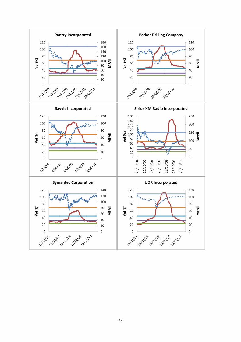
72

0

20

40

60

80

100

120

140

160

180

0

20

40

60

80

100

120

MPAll

Vol (%)

Pantry Incorporated

0

20

40

60

80

100

120

0

20

40

60

80

100

120

MPAll

Vol (%)

Parker Drilling Company

0

20

40

60

80

100

120

0

20

40

60

80

100

120

MPAll

Vol (%)

Savvis Incorporated

0

50

100

150

200

250

020406080100120140160180

26/10/04

26/10/05

26/10/06

26/10/07

26/10/08

26/10/09

26/10/10

MPAll

Vol (%)

Sirius XM Radio Incorporated

0

20

40

60

80

100

120

140

0

20

40

60

80

100

120

MPAll

Vol (%)

Symantec Corporation

0

20

40

60

80

100

120

0

20

40

60

80

100

120

MPAll

Vol (%)

UDR Incorporated

Documents

PRICING CONVERTIBLE BONDS Jonathan A. Batten, Karren Lee