Price and Brand Competition between Differentiated Retailers: a

10-159

Research Group: Industrial Organization April, 2010

Price and Brand Competition between Differentiated Retailers: a Structural Econometric Model

PIERRE DUBOIS AND SANDRA JODAR-ROSELL

Price and Brand Competition between Differentiated Retailers:

A Structural Econometric Model

Pierre Dubois∗and Sandra Jódar-Rosell†

This version: April 2010‡

Abstract

We develop a model of competition between retailer chains with a structural estimation of

the demand and supply in the supermarket industry in France. In the model, supermarkets

compete in price and brand offer over all food products to attract consumers, in particular

through the share of private labels versus national brands across all their products. Private

labels can serve as a differentiation tool for the retailers in order to soften price competition.

They may affect the marginal costs of all products for the retailer because of eventual quality

differences and also by helping retailers to obtain better conditions from their manufacturers.

Differentiation is taken into account by estimating a discrete-continuous choice model of

demand where outlet choice and total expenditures are determined endogenously. On the

supply side, we consider a simultaneous competition game in brand offer and price between

retailers to identify marginal costs. After estimation by simulated maximum likelihood,

the structural estimates allow to simulate the effect on the equilibrium behavior of retailer

chains of a demand shock through an increase in transportation costs for consumers and a

merger between two retailer chains.

JEL Codes: L13, L22, L81

Key words: competition, discrete/continuous choice, retailing, structural estimation

∗Toulouse School of Economics (GREMAQ, INRA, IDEI). [email protected]†Toulouse School of Economics (GREMAQ, INRA). [email protected]‡We thank Rachel Griffi th, Howard Smith, Frank Verboven, Michael Mazzeo, Claire Chambolle, Helena Per-

rone, Thibaud Vergé, Laurent Linnemer, Massimo Motta, Philippe Février, Bruno Jullien, Stéphane Caprice,Vincent Réquillart and seminar participants in Toulouse, IESE Business School, Barcelona, Ecole Polytechniquein Paris, at the workshop on Advances in the empirical analysis of retailing, WZB, Berlin, at EARIE confer-ence at the university of Amsterdam, at INRA-IDEI conference in Toulouse, ASSET conference in Florence,LACEA conference in Rio de Janeiro, EARIE conference in Ljubljana, and the "Jornadas des Economia Indus-trial" conference in Vigo. We also thank Christine Boizot for helping us access the data on France from TNSWorldpanel.

1

1 Introduction

Private labels (PLs), or store brands, have been growing in importance within the food retailing

industry during the last years. Several explanations can be found to justify why a retailer

may find profitable to introduce a PL in its offer. The most common justification in the IO

literature lies in the vertical relationship between manufacturers of National Brands (NBs) and

retailers. In this context, PLs are used by the retailer as a mean to either reduce the double

marginalization problem or to gain some bargaining power in front of manufacturers. The

marketing literature, on the other hand, has stressed the role of PLs as a tool for either better

price discriminate among consumers or for generating consumer loyalty to the store.

All these explanations are in line with statements made by industry managers. Bergès-

Sennou, Bontems and Réquillart (2004) cite a survey by LSA/Fournier1 according to which

the main reasons retailers develop PLs are: to increase customer loyalty (16%), to improve

their positioning (18%), to improve margins (25%) and to lower prices (33%). More direct

conversations with managers reveal that, at least for some retailers, PLs were developed as an

instrument to fight back the entry of Hard Discounters (HDs) in the industry2.

The purpose of this paper is to integrate these considerations in a single framework in order

to better describe how PLs affect the competition between retailers. From their point of view,

private labels play a role both in the demand and in the supply sides. Hence, a complete

evaluation of the impact of PLs in retailer competition needs to take into account both of them.

We will follow the literature on structural models of competition (see, for example, Berry,

Levinsohn and Pakes (1995), Nevo (2001), Ivaldi and Verboven (2005) or Bonnet and Dubois

(2010)) to estimate the parameters of the demand that, together with an assumed equilibrium

condition for the game played by the retailers, will yield estimates for the margins and marginal

costs of each retailer. In order to account for the possible effects of private labels on the supply

side, we will endogenize the location of retailers in the characteristics space defined by the

policy towards PLs. Draganska and Jain (2005) have a similar game of simultaneous price and

product line length competition for the supply side, where the product line is a characteristic

of the market for yogurts analyzed.

The role of private labels on the demand side is two-fold. On the one hand, PLs serve as a

1LSA/Fournier “Les marques de distributeurs”, Libre Service Actualités, 1472 (January 1996):10-15.2This is the case, for example, of Leclerc in France who changed its policy towards PLs in 1998 after the

successful entry of Aldi and Lidl to the french market.

2

differentiation tool for retailers. In the characteristics approach to product differentiation, each

consumer has an ideal mix of private labels and national brands in the assortment of the retailer.

These ideal points are dispersed along the characteristics space, in which retailers themselves

locate by choosing their policy towards these kinds of products. Consumers with stronger

preferences for PLs will naturally choose to visit those retailers offering a larger assortment of

them. Thus the differentiation aspect of PLs comes into play in retailers’competition for the

customers. Once the customers are in the store, PLs play a second role of price discrimination

in each of the product lines offered by the retailer. In this case, the private label is an option

that the retailer can use to better screen the willingness to pay of the different consumers in

its customer base (see Putsis (1997) and Stole (2005)). These two mechanisms also explain

why PLs emerged as a response to the entry of hard discounters: consumers with the lowest

willingness to pay for NBs were attracted by stores offering cheap PL products, reducing the

customer base of the incumbent retailers. Retailers had then the choice between a smaller

customer base but with a higher average willingness to pay - given that entrants provided the

screening device - or keeping the customer base and pursuing themselves the screening through

the introduction of private labels.

To determine whether the development of private labels is an important tool of differentiation

among retailers, we estimate a discrete-continuous choice model for the demand side (following

Haneman (1984) and Smith (2004)) where consumers choose which retailer they patronize and

how much they spend depending on the retailers’characteristics.

A survey published in a study ordered by the Offi ce of Fair Trading about competition in

the retailing industry3 identified the principal factors affecting the choice of a grocery store.

Low price was classified in the third place, just behind the product range and selection and

immediately after the quality of the service. The main factor driving the choice was conveni-

ence. This points out a moderate importance of price competition and shows that retailers are

differentiated according to location and product selection. The strategy of the retailers towards

PL products affects this last factor of differentiation, thus raising the possibility that some

features of this strategy contribute to soften even more the competition in prices. Hence, we

estimate the determinants for patronizing a retailer, and the consumer’s expenditure at it, as

a function of prices, retailer’s and consumer’s characteristics. The effect of PLs as a potential

differentiation device is captured through variables reflecting each retailer’s general PLs policy

3Offi ce of Fair Trading, "Competition in Retailing", Research Paper no 13, September 1993. See section 2.2.3on Consumer relationhips.

3

- the percentage of its offer devoted to PL varieties, the number of product lines with a PL

presence and other characteristics. These variables are included in the store characteristics. In

this way, we can estimate their effect on the consumers’valuation of the bundles that can be

purchased at each retailer.

Following Smith (2004) in the functional form chosen for the indirect utility, we carefully

model the heterogeneity of consumer preferences. However, in Smith (2004), retailer prices are

treated as an unobservable in the estimation of the choice model because of the lack of data on

retailer prices, thus instead of inferring marginal costs, Smith (2004) assumes a multi-store Nash

pricing equilibrium on the supply side and uses aggregated data on marginal costs to estimate

the price parameters using the theoretical expression for the profit margins. Our situation is

the opposite, as it is usual in the literature, given the fact that our database is richer and

records the prices of all the products purchased in any retailer, allowing a direct estimation

of the conditional demand elasticity, which is not the case in Smith (2004). In Smith (2004),

unobserved prices affect retailer choice and expenditures and thus both price parameters are not

identified. Instead, identification is achieved by fixing the value for the ratio of these parameters

so that it implies a plausible conditional (on retailer choice) demand elasticity.

With the estimates of the discrete-continuous choice model at hand, we can compute the

demand observed by each retailer. Assuming a Nash equilibrium in prices in the game played

by the firms owning the different retailers chains, we can express the vector of retailers’margins

as a function of demand parameters. From these margins, we can recover each retailer’s mar-

ginal cost, which reflects a combination of all products’wholesale prices plus marginal costs of

distribution.

Nevertheless, and also given the particular characteristics of the French retailing sector, it is

interesting to consider competition along more than one dimension. French regulation forbids

the resale at a loss for retailers4: the retailer cannot set the price of the good below the price

appearing on the bill from the supplier. All rebates and reductions, i.e. listing fees, payable at

the end of the year but anticipated by the retailers cannot be deduced from the price appearing

in the bill. Moreover, as general terms of sale have to be non-discriminatory according to

commercial law, the effect of the ban on resale at a loss is equivalent to allowing floor prices:

manufacturers can collude to increase wholesale prices and pay the retailers through negotiated

4Resale at a loss was introduced with the Galland Law in 1996 and mostly unchanged until 2006 while ourdata are form 1998-2000. Several studies, including one carried over by the French Competition Authorities,recognized an inflationary effect of the law.

4

listing fees (Allain and Chambolle (2005)). As evidence of this phenomenon, Bonnet and Dubois

(2010) have shown empirically that resale price maintenance was used in the market for bottled

water in France during the years 1998-2000. In this case, price competition between retailers is

significantly restricted and they have to find other dimensions in which to compete. Competition

along the location in the characteristics space, which in this case is a form of competition in

product lines, arises as a reasonable option. For example, one can think that after a merger the

retailers involved may find profitable to reorganize their offers of PLs and NBs in order to better

discriminate among consumers and reduce competition between them (Gandhi et al. (2005)).

Retailers’decisions on their location in the PLs policy space can also be motivated by the

possible different effect of national brands or private labels on the wholesale prices offered by

the manufacturers. Literature on the vertical relationship between manufacturers and retailers

has pointed to two different ways by which PLs can help to obtain lower wholesale prices on

branded products: when linear pricing is used to set wholesale prices, the introduction of a PL

by the retailer reduces the double-marginalization problem (Mills (1995) and Bontems, Monier

and Réquillart (1999)); if non-linear pricing is used instead, Rey and Vergé (2010) show how

they offer the possibility to refuse the contracts proposed by the manufacturers, increasing the

pay-off of non-contracting and thus the rent to retailers.

We thus propose a simultaneous location-and-price game between retailers and assume their

marginal costs to be a function of the mix of national brands and private labels in their assort-

ment. This framework allows to simulate retailers’response to changes in demand or supply

conditions like a transportation cost shock on consumers or a merger among retailers, and com-

pute their effect on their level of prices and product mix, taking into account the possible effect

on costs.

The paper is organized as follows. Section 2 presents a brief review of the literature on

private labels. Section 3 presents the formal description of the model of consumer choice of

a retailer and the likelihood function. The different equilibrium assumptions are discussed in

section 4. Section 5 presents an introduction to the dataset. Section 6 presents the econometric

method and estimation results. Finally, section 7 details the simulation of demand shocks and

merger on equilibrium behavior of retailers.

5

2 Review of the literature

Literature on the effects of PLs on competition has analyzed mainly the relationship between

retailers and manufacturers through their branded products (or NBs). According to this stream

of literature, retailers would introduce PLs in order to increase their bargaining power vis à vis

manufacturers.

In a vertical structure with one manufacturer and one retailer, both in a monopoly position,

if only linear prices are considered (Mills (1995), Bontems et al. (1999)), then this structure

suffers from the double marginalization problem. In this case, by introducing a PL, the retailer

creates competition in the downstream market which reduces the manufacturer’s market power.

Consequently, the wholesale price decreases and so does the double marginalization problem.

Consumer’s surplus rises unless the cost of producing the PL is too high. When non-linear

tariffs are allowed (Caprice (2000), Rey and Vergé (2010)), the double marginalization problem

disappears, since the wholesale price is set at marginal cost. In this case, the mechanism through

which the retailer gains bargaining power is the reservation profit. Assuming the manufacturer

makes a take-it or leave-it offers, the opportunity to sell a PL creates some profit for the retailer

even if he does not sell the national brand (NB). Thus, for the retailer to accept the offer, the

manufacturer must leave some rents to match the retailer’s reservation profit.

There has been also much interest in determining what is the effect of a PL introduction

on the prices of the NBs. Theoretical works tend to favour the prediction of a decline in NB’s

prices whereas empirical works have shown more mixed results. Gabrielsen, Steen and Sørgard

(2001) find a positive effect (when significant) of a PL introduction on the prices of NBs. This

effect is larger for high and moderately successful PL introductions and larger on leading brands.

Regarding the effect of PL penetration on individual NB prices per category, Ward et al. (2002)

find that NB prices tend to rise with PL share and this increase varies within NBs. In some

categories the price increase is much higher in the leading brand and in others it is much

higher in the second or third brands. More recently, Bontemps et al. (2005), using a similar

methodology, show that the positive impact on NB prices is higher for increases in the market

share of PL products stricto sensu. For other kind of PL products - those exclusively sold by

hard discounters or those that are low price products - the effect on NB prices is negative in

half of the categories with significant effects and, in any case, their effect is lower than that of

strictly PL products.

The other reasons stated for introducing a PL have more to do with the horizontal rela-

6

tionships between retailers and have been the subject of less attention in the literature. They

concern the positioning of retailers’offer and customer loyalty. On the theoretical side, Cor-

stjens and Lal (2000) take this approach and try to "show when and why the store brand can

become a source of store loyalty for the retailer". They show that even when there is no cost

advantage with respect to NBs, retailers may find profitable to introduce a PL with a relat-

ively high perceived quality since it is capable of creating store loyalty. Conversely, low cost

low price PLs only increase price competition between retailers. Basically, a PL works as a

brand that is under exclusive distribution in a single retailer. If there exists a certain level

of brand-loyalty for this PL, this loyalty is directly translated into a retailer-loyalty. This is

then a source of switching costs for the consumers, leading to the usual pricing situations and

trade-offs described by Klemperer (1995) of firms facing consumers with switching costs. This

intuition would be in line with the empirical findings of a raise in NB prices after the introduc-

tion of PL varieties. Moreover, empirical results by Bonfrer and Chintagunta (2004) support

the mechanism explained by Corstjens and Lal (2000). They use a panel of 104 product cat-

egories for five competing retailers in one region and construct measures of brand loyalty, store

loyalty and store brand purchase. They find that store loyal consumers are more likely to buy

PL varieties. Higher store loyalty is associated with lower brand loyalty within a store and also

with lower store-invariant measures of brand loyalty. This last correlation suggests that loyal

PL consumers tend to be those with less brand loyalty in general.

Corstjens and Lal (2000) further suggest that consumer’s loyalty to a retailer should be

even higher when he/she opts for purchasing PLs in more than one category of products.

This argument would call for a positive relationship between the retailer’s probability of being

selected and the share of PLs in the total expenditure of the consumer at this retailer. However,

reasons in favour of finding the opposite relationship have also been suggested in the literature.

Sudhir and Talukdar (2004) mention the argument that PLs could attract mainly deal prone

consumers and cite the work of Dick et al. (1995) who find that store brand customers are

more price sensitive than average consumers. Furthermore, if the PL products offered by one

retailer are perfect substitutes for PL products offered by another retailer, then the mechanism

proposed by Corstjens and Lal (2000) for generating retailer-loyalty does not work and the

above mentioned relationship would not exist. Evidence of at least some degree of substitution

is found by Ailawadi and Harlam (2004), who find that retailers’margins on PLs decrease as

the percentage of competing retailers carrying a PL in the category increases.

7

3 Consumer behavior and the demand model

Retailer’s demand is modeled as a combination of discrete and continuous choices. In every

purchasing act, the individual chooses first the retailer and then the quantity purchased at

this particular retailer. These decisions depend on consumer and retailer characteristics. In

particular, since the purchasing act of an individual is motivated by the need of several different

products, the choice of the retailer is going to depend on the prices charged to the different

products sold. We can simplify this by considering that every retailer offers a particular bundle

of goods at a given price. Then, the choice of a retailer is equivalent to purchase one of the

offered bundles.

More formally, and following Haneman (1984), the individual consumer i has a direct utility

function at time t, u defined over the quantities xit = (xi1t, ..., xiJt) of the bundles goods

proposed by Ji different retailers, and on the numeraire qit (which will represent the amount

left for top-ups and other purchases in second choice retailers or other minor retailers included

in the database). Ji is the choice set in terms of retailers for each consumer i. The quantity

xijt represents the quantity of the composite good bought by consumer i at retailer j in period

t. The consumer’s utility also depends on L characteristics of the retailer where the purchase

is made, which will be denoted by b = (b1, ..., bL), and that could vary with the individual

(think of distance to the store for example). Finally, the utility can also be influenced by

M characteristics of the individual, z = (z1, ..., zM ). The vector ε is going to collect all the

characteristics of the retailer and the individual that are unobservable for the econometrician.

At every period t, the individual consumer maximizes his direct utility function u(xit, qit, bijt, zit, εijt)

subject to Ji non-negativity constraints (one for each xijt) and the budget constraint:

Ji∑j=1

pjtxijt + qit = yit

where yit is the consumer’s total expenditure in food and pjt the retail price of store bundle j.

Discreteness in the consumer’s decision comes from the additional constraint that all but one of

the non-negativity constraints must bind because of the necessarily exclusive consumer choice

of retailer. Given this, the problem reduces to choose the pair (xijt, qit), with the other xilt’s

set to 0. This maximization yields a demand function xijt(pjt, yit, bijt, zit, εijt) and an indirect

utility function of the form vijt(pjt, yit, bijt, zit, εijt), both conditional on the purchase of the

bundle belonging to the jth retailer. The selection among the different retailers is made from a

8

choice set Ji, defined as the set of all the retailers present less than 16 km away from consumer

i, and it will be given by the following condition:

vijt(pjt, yit, bjt, zit, εijt) ≥ vikt(pjt, yit, bijt, zit, εijt) ∀k ∈ Ji

The outcome of this selection process is random from the point of view of the econometrician

because of the unobservability of ε. Therefore, the different choices will be observed with a

probability induced by the distribution of ε. The next step in the analysis is to specify a

functional form for the conditional indirect utility function. We use the same functional form

as Smith (2004), which is in turn very close to the one used in Dubin and McFadden (1984)

or Haneman (1984). Treating Roy’s identity as a partial differential equation, this functional

shape belongs to the class of functions that provides a linear in income conditional expenditure

function. Moreover, we specify the way prices and characteristics affect the indirect utility

function such that the conditional expenditures functions be linear in parameters as in Dubin

and McFadden (1984). The additional restriction put on this class of indirect utility functions

is that it provides also a simple and tractable form for discrete choice probabilities.

Accordingly, the conditional indirect utility function has the following shape:

vijt = µ[βg(i)2 yit + β

g(i)1 ln pjt + z′itα

g(i) + ψg(i)1jt

]exp

[(φg(i)2h(j) − β

g(i)2 ln pjt)ζit

]+ ψ

g(i)2ijt + εijt

where g identifies types of consumers with identical preferences, g(i) is the group type of i,

h(j) is the company group to which retailer j belongs to, µ is a scaling term, zit is a vector of

individual characteristics and ψg(i)1jt and ψg(i)2ijt are retailer quality indexes defined as:

ψg(i)1jt = φ

g(i)1h(j) + b′1jtδ

g(i)

ψg(i)2ijt = b′2ijtθ

g(i)

The reason for having two different indices is that some of the retailer characteristics included

in b2ijt - and which may be faced differently by each individual - are not going to influence the

demanded quantity of the bundle. This specification allows to have an individual-store index

ψg(i)2ijt that will not affect the conditional demand functions but affect the probabilities of the

consumer of choosing a given store, and a store specific sort of "quality" index ψg(i)1jt affecting

the conditional demand of the consumer, including eventually an unobserved component φg(i)1h(j)

9

which is fixed over time. Additionally, φg(i)2h(j) is a retailer chain group fixed effect capturing

all those fixed unobserved characteristics of retailer j that only affect the consumer’s choice of

retailer but not the conditional expenditure. Heterogeneity in consumer tastes is introduced

by estimating different sets of parameters Θg = (βg1, βg2, α

g, φg1h, φg2h, δ

g, θg) for every consumer

type g.

Individual’s indirect utility is also affected by unobservable personal characteristics, such as

consumption habits, captured through the univariate random variable ζit and which is assumed

to follow a log-normal distribution LN(0, λg)5. The other source of randomness are unobserved

disturbances to individual’s valuation of retailer j at time t, denoted by εijt, and assumed to be

an i.i.d Type-1 Extreme Value distribution function in standard form with unit scale parameter.

In addition, these two random variables are assumed to be independent.

The application of the Roy’s identity results in the following conditional demand for con-

sumer i at time t for a bundle from retailer j:

xijt =1

pjt

[(βg(i)2 yit + β


g(i) + ψg(i)1jt

)ζit −

βg(i)1

βg(i)2

](1)

and multiplying it by its price, we obtain the conditional expenditure:

eijt =(βg(i)2 yit + β


g(i) + ψg(i)1jt

)ζit −

βg(i)1

βg(i)2

(2)

From the above expressions, it can be seen that characteristics included in ψg(i)2ijt do not

affect the conditional demand and, therefore, the expenditure. These are likely to be retailer

characteristics such as the distance from the consumer’s home or retailer services like the number

of cashiers. The retailer fixed effects capture retailers’characteristics that are constant through

time like, for example, retailers’reputation.

At last, one can also obtain the conditional probability for individual i to choose retailer

j. Actually, given the additivity assumption for εijt on the indirect utility function and the

assumption that εijt follows an extreme value distribution, the probability sijt of retailer j to

be selected by individual i - conditional on the unobserved individual i’s characteristics ζit -

5Hence, E [ζit] = eλg/2 and V ar [ζit] = eλ

g(eλ

g − 1)where g = g(i) is the type of consumer i.

10

follows a multinomial logit:

sijt (ζit) =exp

{µ[βg(i)2 yit + β


g(i) + ψg(i)1jt

]exp

[(φg(i)2h(j) − β

g(i)2 ln pjt)ζit

]+ ψ

g(i)2ijt

}∑k∈Ji

exp{µ[βg(i)2 yit + β

g(i)1 ln pkt + z′itα

g(i) + ψg(i)1kt

]exp

[(φg(i)2h(k) − β

g(i)2 ln pkt)ζit

]+ ψ

g(i)2ikt

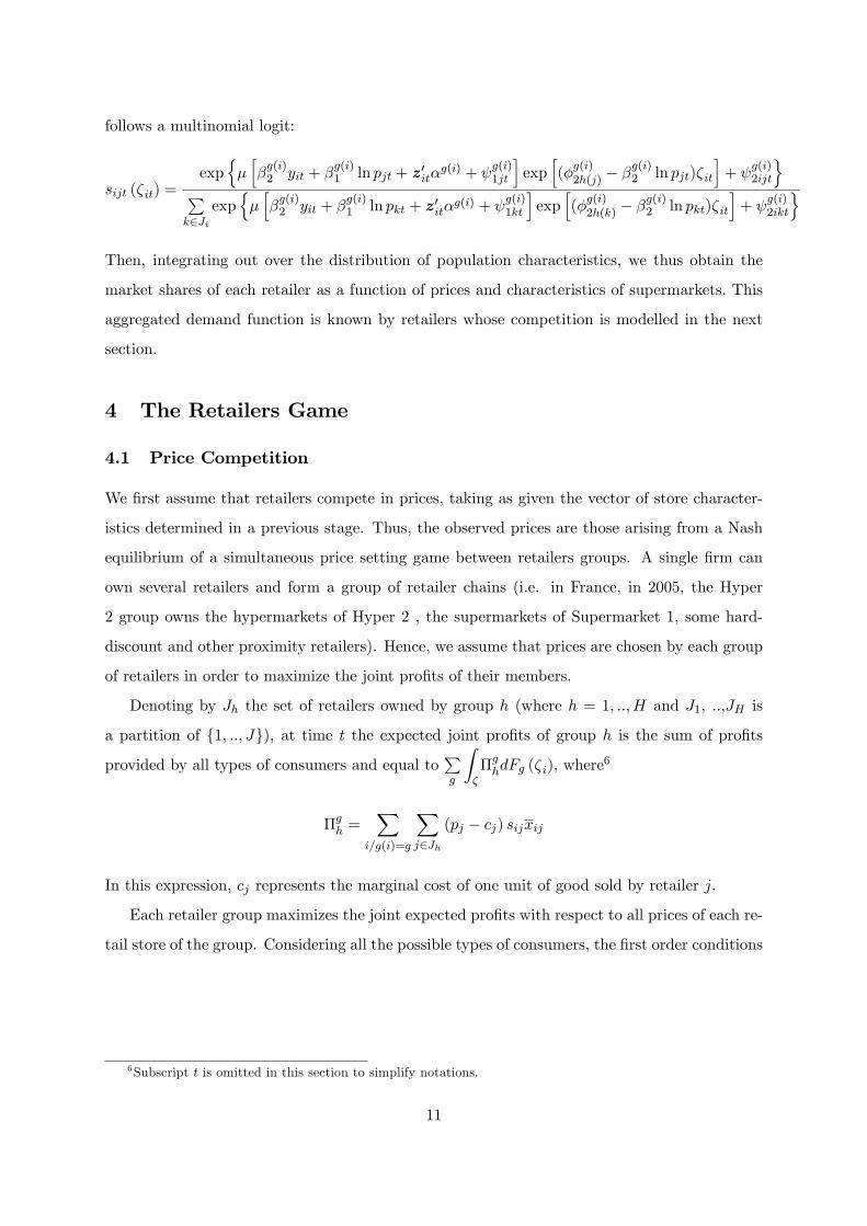
}Then, integrating out over the distribution of population characteristics, we thus obtain the

market shares of each retailer as a function of prices and characteristics of supermarkets. This

aggregated demand function is known by retailers whose competition is modelled in the next

section.

4 The Retailers Game

4.1 Price Competition

We first assume that retailers compete in prices, taking as given the vector of store character-

istics determined in a previous stage. Thus, the observed prices are those arising from a Nash

equilibrium of a simultaneous price setting game between retailers groups. A single firm can

own several retailers and form a group of retailer chains (i.e. in France, in 2005, the Hyper

2 group owns the hypermarkets of Hyper 2 , the supermarkets of Supermarket 1, some hard-

discount and other proximity retailers). Hence, we assume that prices are chosen by each group

of retailers in order to maximize the joint profits of their members.

Denoting by Jh the set of retailers owned by group h (where h = 1, ..,H and J1, ..,JH is

a partition of {1, .., J}), at time t the expected joint profits of group h is the sum of profits

provided by all types of consumers and equal to∑g

∫ζΠghdFg (ζi), where

6

Πgh =

∑i/g(i)=g

∑j∈Jh

(pj − cj) sijxij

In this expression, cj represents the marginal cost of one unit of good sold by retailer j.

Each retailer group maximizes the joint expected profits with respect to all prices of each re-

tail store of the group. Considering all the possible types of consumers, the first order conditions

6Subscript t is omitted in this section to simplify notations.

11

with respect to prices pj of retail group h can be expressed as:

∑g

{∫ζ

∂Πgh

∂pjdFg (ζi)

}= 0 (3)

where∂Πg

h

∂pj=

∑i/g(i)=g

sijxij + (pj − cj) sij∂xij∂pj

+∑k∈Jh

(pk − ck)xik∂sik∂pj

because ∂xik

∂pj= 0 for all k 6= j.

The first term of the summation measures the extra profits coming from the price increase

over the quantity sold. The second term reflects the change in the quantity sold due to the

price increase. This quantity can change through a decrease in the retailer’s probability of

being selected by the consumer but also through a decrease of the consumers expenditure. The

final term captures the effect of a change of retailer j’s prices on the profits of the other retailers

of the group.

Every retailer in group h sets its price level to maximize the sum of the expected profits

derived from each segment of consumers. Thus, the observed price levels must satisfy the system

of J equations formed by the first-order conditions (3). Once the demand is known, the only

unknowns are the marginal costs cj of each retailer, which can be obtained by solving this

system of equations. To see that, the first-order conditions can be expressed in matrix notation.

Define Ih as the ownership diagonal matrix of retail group h, which is of size J × J and

whose elements Ih(j, j) are equal to 1 if retailer j belongs to group h and 0 otherwise. Denote

by ih = diag(Ih) the vector containing the diagonal elements of Ih. Let Sp and Xp be two

J × J matrices containing the sum across consumer types of expected responses of quantity to

a change in prices coming through, respectively, a change in the market share and a change in

the conditional demand, i.e.

Sp ≡

∑

g

{∫ζxi1

∂si1∂p1

dFg (ζi)

}· · ·

∑g

{∫ζxiJ

∂siJ∂p1

dFg (ζi)

}...

. . ....∑

g

{∫ζxi1

∂si1∂pJ

dFg (ζi)

}· · ·

∑g

{∫ζxiJ

∂siJ∂pJ

dFg (ζi)

}

12

Xp ≡

∑

g

{∫ζsi1

∂xi1∂p1

dFg (ζi)

}0 0

0. . . 0

0 0∑

g

{∫ζsiJ

∂xiJ∂pJ

dFg (ζi)

}

Note that the off-diagonal elements of Xp are zero due to our formulation of the conditional

demand, which makes it dependent only on the own-price of the retailer. Finally, define Q as a

diagonal matrix whose diagonal elements are the expected total quantity sold by each retailer

j: Q(j, j) =∑

g

{∫ζsijxijdFg (ζi)

}. Then, the margins γh ≡ [(pj − cj) 1j∈Jh ]j of retailers of

group h (1j∈Jh = 1 if j ∈ Jh and 0 otherwise) are solution of the following equations:

Qih + (IhXp + IhSpIh) γh = 0 ∀h = 1, ..,H (4)

The solution to this system of equations can be found by minimizing the sum of squares of

condition (4). This yields a solution for γh of the form, ∀h = 1, ..,H:

γh = − (IhXp + IhSpIh)−1Qih (5)

When solving the system of J equations, we obtain an estimate for the marginal cost of each

store bundle of goods. This estimate is of course dependent on the assumption about the game

that is played by the retailers. Were the retailers engaged, for example, in tacit collusion, the

real marginal costs would differ from those estimated here.

4.2 Simultaneous Location-and-Price Competition

Suppose now that retailers compete not only in prices but also in their location choice in

the characteristics space of goods, choosing both variables simultaneously. More specifically,

retailers can vary their offer in PL and NB so as to attract more consumers to the store and,

possibly, increase expenditures. This kind of game implies a second set of first-order conditions

that adds to the set defined in (3), which allows us to recover more information on the parameters

determining retailers’marginal costs.

Literature on the vertical relationship between manufacturers and retailers has signaled the

importance of PLs in the outcome of this relationship. When linear pricing is used to set

wholesale prices, the introduction of a PL by the retailer reduces the double-marginalization

problem and allows the retailer to purchase NBs at a lower wholesale price. If non-linear

13

pricing is used instead, PLs can be used by the retailers to increase their market power within

the vertical structure. Rey and Vergé (2010) show how they offer the possibility to refuse the

contracts proposed by the manufacturers, since retailers can rely on other manufacturers and

on their PLs to conform their offer. Moreover, the wider the coverage of PL brands the easier to

refuse contracts that bundle several brands of the manufacturer. Since PLs increase the payoff

of non-contracting, the manufacturer is obliged to leave a positive rent to the retailer. This

rent depends inversely on the retailer’s profit on the other brands and can be affected by the

manufacturer through the wholesale price offered to the retailer.

In order to test whether PL brands have a different impact than NBs on retailers’marginal

costs, we consider that their marginal cost function depends on the ratio in which each type of

brands is present in their assortment. Denote this ratio by ρj . Therefore, in the simultaneous

location-and-price game, retailers forming the group h solve the following problem:

Max{pj ,ρj}j∈Jh

∑g

{∫ζΠghdFg (ζi)

}≡∑

g

∫ζ

∑i/g(i)=g

∑j∈Jh

(pj − cj

(ρj))sij (p, ρ)xij

(pj , ρj

)dFg (ζi)

Each retailer then chooses the level of its ρj according to its effect on market shares, condi-

tional demands and marginal cost levels. We do not need to impose any functional form for the

relationship between this ratio and the level of marginal costs. Actually, this ratio can affect

marginal costs in two ways: a) it may reduce the marginal cost of the bundle of products by

substituting branded product varieties by PLs that may be purchased at lower wholesale prices;

b) it may reduce the wholesale price for other NBs by increasing the rent that manufacturers

are obliged to leave to the retailer. Note, as well, that the level of marginal costs may depend

on factors that are known for the retailers but unobserved by the econometrician - i.e. the

retailer’s ability to negotiate contracts or any bargaining power vis a vis manufacturers and

orthogonal to ρj . Assuming that there is a unique maximum, we use the first-order conditions

with respect to price which are given by equation (3) and the one with respect to ρj . Actually,

the maximization with respect to ρj yields the following additional conditions:

∑g

{∫ζ

∂Πgh

∂ρjdFg (ζi)

}= 0 (6)

where the derivative of retail group h’s profits arising from consumers of type g with respect to

14

the ratio is given by the following expression, for all j ∈ Jh, and h = 1, ..,H

∂Πgh

∂ρj=

∑i/g(i)=g

−sijxij ∂cj∂ρj

+ (pj − cj) sij∂xij∂ρj

+∑k∈Jh

(pk − ck)xik∂sik∂ρj

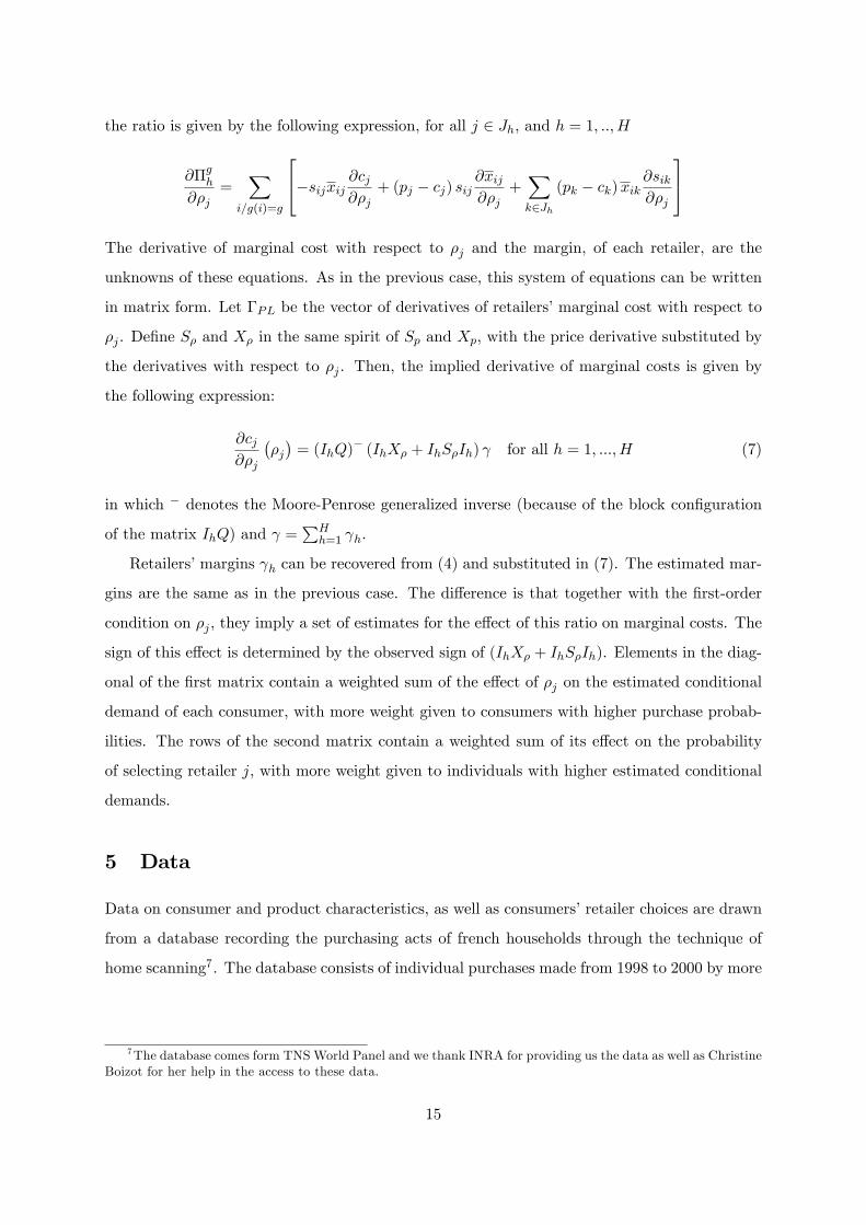
The derivative of marginal cost with respect to ρj and the margin, of each retailer, are the

unknowns of these equations. As in the previous case, this system of equations can be written

in matrix form. Let ΓPL be the vector of derivatives of retailers’marginal cost with respect to

ρj . Define Sρ and Xρ in the same spirit of Sp and Xp, with the price derivative substituted by

the derivatives with respect to ρj . Then, the implied derivative of marginal costs is given by

the following expression:

∂cj∂ρj

(ρj)

= (IhQ)− (IhXρ + IhSρIh) γ for all h = 1, ...,H (7)

in which − denotes the Moore-Penrose generalized inverse (because of the block configuration

of the matrix IhQ) and γ =∑H

h=1 γh.

Retailers’margins γh can be recovered from (4) and substituted in (7). The estimated mar-

gins are the same as in the previous case. The difference is that together with the first-order

condition on ρj , they imply a set of estimates for the effect of this ratio on marginal costs. The

sign of this effect is determined by the observed sign of (IhXρ + IhSρIh). Elements in the diag-

onal of the first matrix contain a weighted sum of the effect of ρj on the estimated conditional

demand of each consumer, with more weight given to consumers with higher purchase probab-

ilities. The rows of the second matrix contain a weighted sum of its effect on the probability

of selecting retailer j, with more weight given to individuals with higher estimated conditional

demands.

5 Data

Data on consumer and product characteristics, as well as consumers’retailer choices are drawn

from a database recording the purchasing acts of french households through the technique of

home scanning7. The database consists of individual purchases made from 1998 to 2000 by more

7The database comes form TNS World Panel and we thank INRA for providing us the data as well as ChristineBoizot for her help in the access to these data.

15

than 9000 households8 in french distributors of food products. It covers all the metropolitan

french departements and 476 products belonging to 64 different food categories (water, aperitifs,

fresh fruits, cheese ...)9. It is representative of the French population.

The database is organized as a collection of product files in which a typical record is a

purchase of that product in a given retailer at a certain date. In this record one has information

about the identifying code of the individual, so that we can trace all the purchases of each

individual, his/her socio-demographic characteristics, as well as characteristics of the product

(brand, price, format ...), quantity purchased and retailer characteristics (name of the retailer,

surface of the store and type of retailer).

Since different individuals can have different purchasing habits, and may therefore visit

the stores with a different frequency, observations belonging to the same month are grouped

together. The choice of the period length as a month is somewhat arbitrary, but it is long enough

to capture different habits. Moreover, it will be useful in the construction of price indexes that

will avoid short-term variations due to product promotions and enables us to abstract from

other dynamic considerations.

Data on outlet characteristics for every retailer were obtained from LSA/Atlas de la Dis-

tribution 2005, which lists all the french outlets involved in food distribution. Besides their

location, the Atlas provides us with the name of the retailer chain the outlet is affi liated to,

its surface, the number of cash registers, the number of employees, the number of parking slots

and the number of pumps available in the outlet’s gas station. We merged this information

with the household data using the name of the retailer, the zip code of the consumer’s residence

and the surface of the outlet. For each of the retailer chain, we found the closest outlet to the

consumer dwellings thanks to zip codes and geographical data allowing to compute distances.

If this distance was less than 16 kilometers, the outlet was included in the consumer’s choice

set. Only one outlet per retailer chain was included in this set. The computed distance is added

as an additional retailer characteristic.

Using the information contained in the household data, several additional variables have been

constructed regarding individuals’and retailers’characteristics (from all the possible retailers,

8The number of households for 1998 is of 9756, that of 1999 is 11310, while the same figure for 2000 is of12291. Around 1/4 of the panel is renewed every year, thus leaving us with 3710 households present in the wholeperiod.

9Nevertheless, households do not record all the products purchased. In particular, for each household thereis a group of products not recorded. This group can be either a) fruits and vegetables or b) fish and meat. Therest of products are recorded for all the households.

16

we selected 22 of them representing about a 90% of the total sales recorded in the database).

5.1 Household-specific variables

The data contain detailed information on households characteristics including household com-

position, geographic information on dwellings and also some classification by income groups

that will be used to define groups of consumer types. The data also contain detailed continuous

observation of all purchases with information on products, brands, prices, retailers.

The data on purchase are aggregated at the household level, by month and we define the

following variables:

• Monthly expenditure per retailer : All the purchases of a household during a particular

month are aggregated to form his monthly expenditure. Purchases made at the selected

retailers are identified and the rest of the purchases are aggregated into purchases in the

outside option. The first row of Table 1 presents the average across individuals in the

panel of their total expenditure per month.

• First and second choice retailers: The first choice retailer is the one where an individual

spent the most in a given month. The same computations have been done for the second

retailer choice. The average monthly expenditure across consumers in first and second

choice retailers is displayed in Table 1. For each household, expenditure in PL products

in each retailer is also computed. Table 1 also shows the average of this expenditure

across consumers with a positive purchase, of any kind of product, at first and second

choice retailers.

• Share of PL products in expenditures per retailer: It is the monthly expenditure in PL

products made at a given retailer over the consumer’s total expenditure at that retailer.

This variable reflects the importance of PL products in individuals’average expenditure

per retailer.

• Loyalty to a retailer in terms of first choice: This is a dummy variable indicating whether

an individual’s first choice in a given period coincides with his/her first choice retailer in

the previous period. This variable is shown at the bottom of Table 1.

• Loyalty to a retailer in terms of total expenditures: It is the percentage that the monthly

expenditure spent on a given retailer represents over the total expenditure of the household

across all retailers during that month.

17

(in € ) 1998 1999 2000

Monthly expenditure Mean 173.13 170.62 166.89

St. Dev 137.98 144.96 150.46

Monthly expenditure in 1st choice retailer Mean 128.95 128.52 126.23

St. Dev 119.83 129.16 135.67

Monthly expenditure in 2nd choice retailer Mean 41.96 40.92 39.84

St. Dev 36.00 35.21 34.75

PL monthly expenditure in 1st choice retailer Mean 26.95 28.94 29.38

St. Dev 57.56 74.89 83.77

PL monthly expenditure in 2nd choice retailer Mean 10.02 10.54 10.45

St. Dev 14.37 14.59 14.02

Number of visited retailers Mean 2.97 2.95 2.95

St. Dev 1.09 1.09 1.09

Loyalty to first choice retailer Mean 0.66 0.66 0.64

Table 1: Summary statistics for consumers’data

The data show that the average expenditure in first-choice retailers is significantly larger

than in second-choice ones. This suggests that the selection of the first-choice retailer is the

most relevant decision for the consumer. On the other hand, expenditure in PLs is relatively

more important at second than at first choice retailers. Finally, around 65% of the households

in the sample chose the same retailer in two consecutive periods.

5.2 Retailer-specific variables

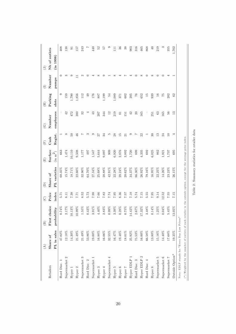
Table 2 shows some statistics at the retailer level over the variables defined as below:

• Sales in PL products: Column (A) displays the retailer specific ratio of sales in PL products

over its total sales (PL penetration).

• First choice probability: Column (B) shows the average probability of choosing a given

retailer as first choice (in terms of expenditures). This is computed as the number of

households who prefer a given retailer spending the largest part of their food expenditures

in that retailer over the total number of households who purchased some food in a given

period.

• Price index: Column (C) shows a price index computed for every retailer using data on

prices and quantities purchased. Details the construction of this index are given in the

following subsection.

• Share of PL varieties in total offer: Column (D) presents the number of PL varieties

(references) offered by the retailer over the total number of varieties offered. The whole

18

offer cannot be observed and, instead, both the numerator and the denominator have to

be computed using the records from the household data. The denominator is computed

as the addition of the number of varieties offered for each product in a particular retailer

chain for each period. We aggregate the information coming from outlets with a similar

surface within a retailer: every outlet is assigned into a group according to its surface

in steps of 50 m2. We divide France in 7 large regions and thus the sum is conducted

by retailer, region, group and period. The computation of the numerator is analogous to

that of the denominator but considering only the references identified as PLs. For hard

discounters, this share is defined as hard discount brands over total varieties offered.

• Share of NB varieties in total offer: Similar to the previous variable but taking into

account only varieties classified as NB. The total number of varieties offered is not equal

to the sum of the number of PL and NB because of the presence of "First Price" brands

or of "Regional" brands.

• Surface, cash registers, employees, car parking, pumps and number of outlets: Columns

(E) to (J) present the averages across retailers of the variables provided by LSA’s Atlas.

19

(A)

(B)

(C)

(D)

(E)

(F)

(G)

(H)

(I)

(J)

Retailers

Shareof

Firstchoice

Price

Shareof

Surface

Cash

Number

Parking

Number

Nbofoutlets

PLinsales

probability

index

PLvarieties

(inm2)

Regist.

employees

slots

pumps

(in1998)

HardDisc.1

47.02%

0.74%

5.71

60.35%

663

1—

90

408

Supermarket2

12.18%

2.17%

8.11

15.74%

1,474

842

159

3138

Hyper1

14.30%

10.13%

7.38

18.71%

10,110

50472

1,790

991

Hyper2

21.49%

10.99%

7.71

22.60%

9,508

46380

1,856

11157

Supermarket3

21.49%

1.55%

8.52

32.90%

1,177

732

112

2243

HardDisc.2

53.86%

0.43%

5.73

64.70%

497

34

490

7

Supermarket1

19.00%

3.91%

7.98

27.34%

1,547

943

176

4440

Hyper3

16.88%

4.40%

7.66

25.68%

5,644

27207

887

852

Hyper4

16.06%

2.83%

7.82

20.88%

9,097

34344

1,199

957

Supermarket4

32.55%

0.99%

7.74

42.91%

909

512

541

9

Hyper5

16.47%

3.39%

7.95

22.28%

6,920

28219

1,089

8111

Hyper6

19.48%

0.28%

8.36

28.24%

2,876

1581

371

436

Hyper7

18.01%

0.75%

7.57

20.62%

3,892

21151

602

738

HyperEDLP1

25.92%

14.42%

7.18

34.37%

1,720

942

205

4903

HardDisc.3

75.53%

2.67%

5.74

86.30%

899

720

760

316

HyperEDLP2

16.00%

17.32%

7.15

26.92%

4,335

22165

652

8465

HardDisc.4

66.58%

3.48%

5.55

79.16%

692

1—

150

868

Hyper8

13.80%

0.14%

7.95

16.95%

6,025

30251

939

840

Supermarket5

15.16%

1.25%

9.14

22.25%

862

1363

160

219

Supermarket6

14.40%

0.04%

12.52

14.26%

1,921

24165

750

3

Supermarket7

17.68%

5.45%

7.55

23.23%

1,737

1056

202

4355

OutsideOption*

19.35%

13.05%

7.15

26.15%

695

413

621

1,702

Note:EDLPstandsfor"EveryDayLowPrices"

(*)Weightedbythenumberofoutletsofeach

retailerintheoutsideoption,exceptfortheaverageprice

index.

Table2:Summarystatisticsforretailerdata

20

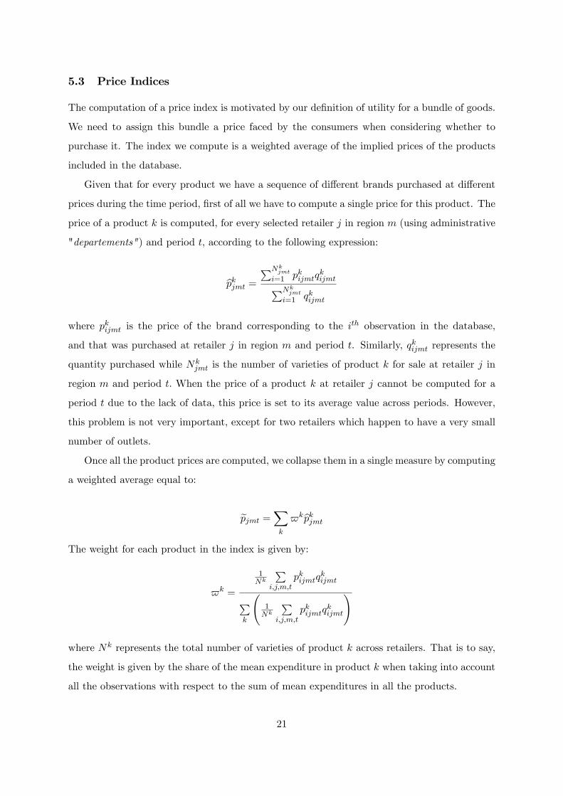
5.3 Price Indices

The computation of a price index is motivated by our definition of utility for a bundle of goods.

We need to assign this bundle a price faced by the consumers when considering whether to

purchase it. The index we compute is a weighted average of the implied prices of the products

included in the database.

Given that for every product we have a sequence of different brands purchased at different

prices during the time period, first of all we have to compute a single price for this product. The

price of a product k is computed, for every selected retailer j in region m (using administrative

"departements") and period t, according to the following expression:

pkjmt =

∑Nkjmt

i=1 pkijmtqkijmt∑Nk

jmt

i=1 qkijmt

where pkijmt is the price of the brand corresponding to the ith observation in the database,

and that was purchased at retailer j in region m and period t. Similarly, qkijmt represents the

quantity purchased while Nkjmt is the number of varieties of product k for sale at retailer j in

region m and period t. When the price of a product k at retailer j cannot be computed for a

period t due to the lack of data, this price is set to its average value across periods. However,

this problem is not very important, except for two retailers which happen to have a very small

number of outlets.

Once all the product prices are computed, we collapse them in a single measure by computing

a weighted average equal to:

pjmt =∑k

$kpkjmt

The weight for each product in the index is given by:

$k =

1Nk

∑i,j,m,t

pkijmtqkijmt

∑k

(1Nk

∑i,j,m,t

pkijmtqkijmt

)

where Nk represents the total number of varieties of product k across retailers. That is to say,

the weight is given by the share of the mean expenditure in product k when taking into account

all the observations with respect to the sum of mean expenditures in all the products.

21

Other price indexes could be computed following Diewert (1976). In particular, the Fisher

price index is exact for a general translog expenditure function. Since the translog functional

form provides a second order approximation to any general expenditure function, it is considered

a good approximation to the true cost of living price index. The computation of the weights

can also be done in different ways. Tests will be done to check the robustness of our results to

these different price indexes.

The use of a price index may also be considered problematic since it may suffer from en-

dogeneity. By construction, the index takes only into account the prices of those varieties of

products finally purchased by the consumer. However, since we are using averages over all the

consumers in the database, we expect this problem to be small. In a first stage, and given that

the retailer choice model is estimated using data at the individual level, we will treat the price

index as exogenous and test this assumption later.

6 Identification and Econometric Method

6.1 Estimation method

Given the functional form chosen for the indirect utility and the distribution of εijt, the prob-

ability of retailer j to be selected by household i - conditional on its unobserved characteristics

ζit - follows a multinomial logit:

sijt (ζit) =exp

{µ[βg(i)2 yit + β


g(i) + ψg(i)1jt

]exp

[(φg(i)2h(j) − β

g(i)2 ln pjt)ζit

]+ ψ

g(i)2ijt

}∑k∈Ji

exp{µ[βg(i)2 yit + β

g(i)1 ln pkt + z′itα

g(i) + ψg(i)1kt

]exp

[(φg(i)2h(k) − β

g(i)2 ln pkt)ζit

]+ ψ

g(i)2ikt

}The unconditional probability of individual i selecting retailer j can be found by integrating

out over the distribution of the unobserved individual characteristics:

rijt =∑

g1g(i)=g

∫ζsijt (ζit) dFg (ζit) (8)

where Fg is the cumulative density function of ζ for type g consumers, assumed to be identically

distributed for all consumers within a type g. As ζ is assumed log normal, this unobserved

individual characteristic also induces a density of the conditional expenditure, which can be

22

found by a change of variable technique:

feijt (eijt | j) =1[

eijt +βg(i)1

βg(i)2

]√2πλ

exp

− 1

2λg(i)

ln

eijt +(βg(i)1 /β

g(i)2

)βg(i)2 yit + β


g(i) + ψg(i)1jt

2

(9)

Therefore, the joint probability of observing consumer i spending an amount of eijt in retailer

j at time t is equal to the conditional probability times the marginal probability and is given

by the product of expressions (8) and (9). The likelihood of the sample is given by the following

expression:

ln L =∑i,j,t

dijt{

ln rijt + ln[feijt (eijt | j)

]}where dijt is a dummy variable indicating whether consumer i chose retailer j at time t or not.

6.2 Specification choices

Let’s choose the variables entering the different elements of the indirect utility. In addition to the

household budget attributed to food (yit) and the price of the basket of goods (pjt), variables b1jt

in ψg(i)1jt are considered to affect both the choice of a retailer and the conditional expenditure of

the consumer. Among them, retailer-specific characteristics include the logarithm of its surface

(ln surface) and the ratio ρj of PL varieties to NBs in its assortment. Fixed effects capture

observable and unobservable characteristics of retailers that are constant across households and

time. The most important of these characteristics is the average perception of retailer’s quality.

zit contains also individual-specific variables such as the number of cars in the household or the

size of the household.

Given the dependence of the estimates of the elasticity of costs with respect to ρj , it is

important to capture as flexibly as possible all the taste variations in the sample. Consumer

taste for ρj is allowed to vary between consumers along two dimensions. First, consumers may

value differently PL varieties sold at hard discounters than those sold at traditional retailers.

Second, due to the earlier entry of hard discounters in the Northern part of France, preferences

for PLs are allowed to vary also between consumers of the north-west and south-east parts of

France.

The term ψg(i)2ijt represents the effect of the variables that may condition the household’s

choice of a retailer but not his expenditures. We include the distance between the household

and the retailer (distance), the logarithm of the surface of the retailer outlets (ln surface) - this

23

is a proxy for the total number of varieties, or the assortment, offered by the retailer at that

outlet - and the number of competing retailers located less than 3 kilometers away from the

consumer.

Finally, a second set of retailer fixed effects is included in φg(i)2h(j) to capture unobservable

retailer chain characteristics that do not influence the conditional expenditure of the individual.

As in Smith (2004), the identification of the two sets of fixed effects is possible because we

observe both the retailer choice and the expenditure for every individual.

Given the complexity of the model to be estimated and to ease the computational burden,

some restrictions have been added implicitly on the valuation of the alternatives for the con-

sumers by gathering all hard discounters and a minor hypermarket chain into two alternatives

(Hard discounters and Other hypermarkets); the outside option is enlarged with the smallest

supermarkets from Table 2. This formulation assumes that retailers within the grouped altern-

atives are perfect substitutes for each other and that their unobserved characteristics, such as

quality, are equally perceived by the consumers within these two kinds of retailers. Hence, the

two alternatives represent the aggregate competitive pressure that hard discounters and the rest

of the minor hypermarkets put on the remaining retailers.

6.3 Identification issues

Demand parameters are obtained using simulated maximum likelihood (SML). Simulated choice

probabilities are computed averaging the results from 60 random draws taken for every obser-

vation from a log-normal distribution LN(0, λg(i)) for ζit.Convergence of the iteration process

that estimates the λg(i) parameters jointly with the rest of demand parameters is hard to obtain

and requires good starting values. However, part of the parameters are already identified with

the conditional expenditure equation (2). In particular, λg(i) is identified and can be estimated

by maximum likelihood estimation of this equation. Thus, similarly to Smith (2004), we follow

a three step procedure in which the estimated value of λg(i) - obtained after the maximum

likelihood estimation of the conditional expenditure - is then used to define the distribution

from which the random draws are taken. All other parameters of the discrete-continuous choice

model are then estimated by SML in a second stage. The third step recomputes the value of

λg(i) that maximizes the SML at the estimated value of the other parameters in step 2. Steps

2 and 3 are repeated until convergence.

As already mentioned, the identification of this discrete/continuous choice model is achieved

24

here with the exclusion restriction that the distances to the retailers affect the choice probabil-

ities of retailers by each consumer but not the conditional expenditure. This is justified by the

fact that we exclude the distance to the retailer to affect the expenditure at that retailer once it

is chosen. Moreover, we consider choice sets for each consumer which depend on the catchment

area (defined using the set of retailer stores present within a given distance to the household

address). These choice sets vary across consumers and we assume that prices and characteristics

of retailers in the choice set vary exogenously with respect to the unobserved consumer taste

distribution conditional on household characteristics like their income group. This amounts to

assume that there is no other heterogeneity of consumer tastes that would be observed by the

retailer when they choose prices.

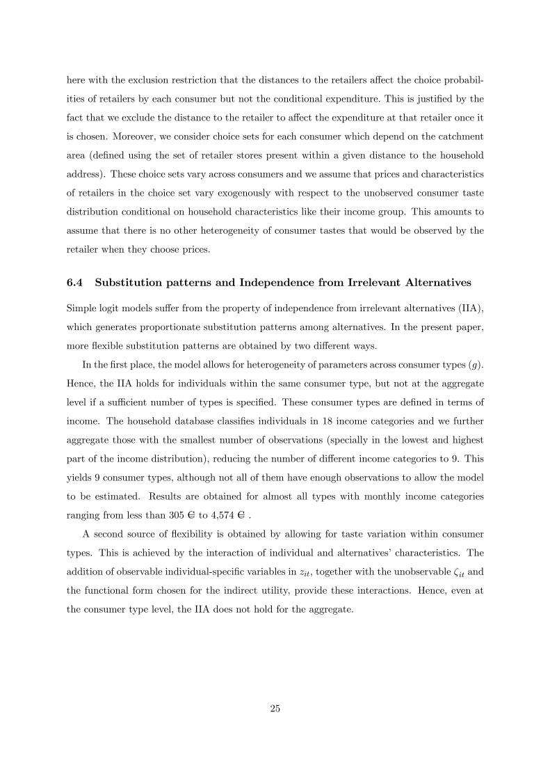
6.4 Substitution patterns and Independence from Irrelevant Alternatives

Simple logit models suffer from the property of independence from irrelevant alternatives (IIA),

which generates proportionate substitution patterns among alternatives. In the present paper,

more flexible substitution patterns are obtained by two different ways.

In the first place, the model allows for heterogeneity of parameters across consumer types (g).

Hence, the IIA holds for individuals within the same consumer type, but not at the aggregate

level if a suffi cient number of types is specified. These consumer types are defined in terms of

income. The household database classifies individuals in 18 income categories and we further

aggregate those with the smallest number of observations (specially in the lowest and highest

part of the income distribution), reducing the number of different income categories to 9. This

yields 9 consumer types, although not all of them have enough observations to allow the model

to be estimated. Results are obtained for almost all types with monthly income categories

ranging from less than 305 C= to 4,574 C= .

A second source of flexibility is obtained by allowing for taste variation within consumer

types. This is achieved by the interaction of individual and alternatives’characteristics. The

addition of observable individual-specific variables in zit, together with the unobservable ζit and

the functional form chosen for the indirect utility, provide these interactions. Hence, even at

the consumer type level, the IIA does not hold for the aggregate.

25

6.5 Simultaneity bias

The estimation of demand for differentiated products may suffer from endogeneity problems

analogous to those posed by homogeneous product analysis: producers will set all the control

variables in their maximization problem (price and ρj , here) taking into account any demand

shocks that they may observe. If these shocks are unobserved by the econometrician, then a

simultaneity bias appears. In the context of differentiated products and discrete choice models,

these shocks are product characteristics (in our case, retailer characteristics) that are unobserv-

able or hardly measurable by the researcher. Among these characteristics, quality stands out

as one of the most important. Other such characteristics proposed in the literature are past

experience (Berry et al. (1995)) or advertising and coupon activity (Besanko et al. (1998)).

To the extent that these characteristics are constant through time, the inclusion of retailer

fixed effects in the indirect utility should remove this source of correlation from the error term.

Hence, the coeffi cients of price and of ρj would be unbiased. On the other hand, advertising or

promotions can be thought as varying in time. Advertising is likely to be higher during weeks

in which there is a promotion. Nevertheless, our time period being a month, we expect these

two variables to be fairly constant through these aggregated time periods and so their effect to

be captured through the fixed effects.

7 Estimation results and simulations

7.1 Empirical estimates of the demand model and margins

Tables 3 and 4 present the results obtained10. Remark that we allow the ratio of private labels to

national brand in the product offerings (ρj) to affect utility differently across two large regions

(the north and northeast of France and the rest of the country) through interactions with

the dummy variable "Northern region" and we also allow this ratio to affect utility differently

between hard discount retailers and "traditional" retailers through the interaction with a dummy

variable for hard discounters. This choice has been the result of a specification search, and

indeed we see from estimates that the offer of more private label products (higher ρj) can

have opposite effects on the utility of consumers depending on their income groups. This taste

10Due to the small market share of Hard discounters among consumers of types 6, 7 and 8, the estimation forthese groups has been performed excluding Hard discounters from the possible alternatives. Also, the estimationfor group 5 failed to converge and hence it is not reported. Remark also that some variables have been removedfrom the specification of utility on an empirical basis.

26

variation can be interpreted in several ways but reflects the fact that private label products can

be perceived differently in the population. Given the functional form chosen for the utility of

the consumer, the interpretation of the coeffi cients cannot be read directly from the table. The

exception are the coeffi cients of variables inside ψ2jt, which enter the utility function linearly.

As expected, distance to the retailer reduces the utility of every alternative. Its effect is less

severe for middle-income consumers, who are more willing to travel. Low-income consumers

may face high transportation costs whereas high-income consumers may value more their time.

The surface of the retailer has a positive effect on the utility for nearly all the income classes,

but less so for the high-income consumers. On the contrary, these consumers have a higher

valuation for the availability of parking slots. With respect to the availability of gas stations,

when significant, results show that it is positively valued. This is specially true for low and

middle-income consumers. Finally, a higher number of retailers close to the consumer reduces

the mean utility that he derives from each of them.

The estimated parameters also allow to compute the corresponding elasticities that are

presented for each retailer in Table 5.

27

Groupdependent

Group0

Group1

Group2

Group3

parameters

Coeff.

StdErr.

Coeff.

StdErr.

Coeff.

StdErr.

Coeff.

StdErr.

µ-1.6449

55.7574

1322.30

813.47

2907.00∗∗

1476.36

4003.67∗∗∗

1514.40

β1

17.646∗∗∗

5.8421

19.109∗∗∗

3.5515

23.0657∗∗∗

3.1411

21.3423∗∗∗

2.6881

β2

0.6874∗∗∗

0.0129

0.706∗∗∗

0.0076

0.7215∗∗∗

0.0053

0.6925∗∗∗

0.0043

ψ1

Hyper1

-13.051

70.857

-38.331

24.060

-102.147∗∗∗

23.507

20.120

20.363

Hyper2

21.259

71.254

-32.455

24.297

-106.395∗∗∗

23.834

21.370

20.716

Supermarket1

40.868

62.987

-11.428

21.733

-101.442∗∗∗

21.740

12.359

19.144

HyperEDLP1

30.125

68.873

-0.733

22.044

-84.553∗∗∗

22.158

42.158∗∗

19.165

HyperEDLP2

27.764

68.735

-12.141

22.882

-87.891∗∗∗

22.599

34.462∗

19.658

Others

38.149

58.917

-6.591

20.705

-71.313∗∗∗

20.246

35.599∗∗

17.572

OtherHyperm.

-8.610

69.229

-16.975

23.690

-92.635∗∗∗

23.724

16.872

20.421

HardDiscount

259.244

342.977

-162.47∗∗∗

23.579

-176.827∗∗∗

20.460

-123.97∗∗∗

19.001

ρj

-33.8439

48.3953

8.5547

10.3760

19.8202∗

10.4626

-11.1250

9.4022

ρj×Nothernregion

-32.028∗∗∗

10.6108

-7.8773

5.6836

-17.1569∗∗∗

5.2063

-10.9406∗∗

4.4362

ρj×HardDiscount

9.4401

55.8011

5.8313

10.4256

-8.8196

10.5012

26.3282∗∗∗

9.4221

ρj×Nothernregion×HardDisc.

28.662∗∗

11.5323

8.0043

5.4687

17.4546∗∗∗

5.0231

9.5219∗∗

4.2711

αHouseholdsize

-1.2674

3.3536

2.7329

1.9293

-0.0559

1.4498

-0.3615

1.2828

Numberofcars

2.7973

4.7848

4.6193

3.5382

-1.3316

2.7039

4.8674∗

2.6876

Logsurface

-0.2704

7.0307

-1.9008

2.4860

6.6603∗∗∗

2.4056

-4.7680∗∗

2.1848

φ2

Hyper1

-8.2801

37.7343

-6.781∗∗∗

0.5417

-7.7008∗∗∗

0.4510

-8.0726∗∗∗

0.3338

Hyper2

-4.2704

31.2911

-6.798∗∗∗

0.5425

-7.6985∗∗∗

0.4511

-8.0887∗∗∗

0.3344

Supermarket1

-3.1689

29.2542

-6.804∗∗∗

0.5413

-7.7204∗∗∗

0.4514

-8.0733∗∗∗

0.3333

HyperEDLP1

-4.5623

30.5571

-6.833∗∗∗

0.5407

-7.7227∗∗∗

0.4505

-8.0927∗∗∗

0.3331

HyperEDLP2

-5.1305

31.2748

-6.839∗∗∗

0.5418

-7.7370∗∗∗

0.4507

-8.1070∗∗∗

0.3336

Others

-5.3460

27.3536

-6.764∗∗∗

0.5416

-7.6684∗∗∗

0.4504

-8.0457∗∗∗

0.3331

OtherHyperm.

-5.3272

29.6074

-6.776∗∗∗

0.5419

-7.7099∗∗∗

0.4506

-8.0699∗∗∗

0.3337

HardDiscount

-2.8311

28.7772

-7.029∗∗∗

0.5408

-7.9590∗∗∗

0.4503

-8.3107∗∗∗

0.3327

ψ2

Distance

-0.5286∗∗∗

0.0500

-0.513∗∗∗

0.0197

-0.4843∗∗∗

0.0147

-0.3918∗∗∗

0.0109

Logsurface

-0.3079

0.2304

0.379∗∗∗

0.0828

0.2533∗∗∗

0.0562

0.4831∗∗∗

0.0550

Nbretail<3km

-0.2362∗∗∗

0.0703

-0.434∗∗∗

0.0478

-0.3770∗∗∗

0.0337

-0.4733∗∗∗

0.0276

Nbcashier/m2

0.0299∗∗∗

0.0070

-0.0041

0.0049

0.0088∗∗∗

0.0034

0.0195∗∗∗

0.0026

Nbpark.slot/m2

-1.9377∗∗∗

0.2768

-0.5508∗∗∗

0.1572

-1.0115∗∗∗

0.1239

-0.4939∗∗∗

0.0931

Nbpumps/m2

1.6690∗∗∗

0.3949

-0.0166

0.2316

1.1736∗∗∗

0.1774

-0.1623

0.1525

λ0.0718∗∗∗

0.0059

0.0768∗∗∗

0.0041

0.0796∗∗∗

0.0029

0.0812∗∗∗

0.0024

Table3:Resultsofthediscrete-continuouschoicemodelpergroupsofconsumers

28

Groupdependent

Group4

Group6

Group7

Group8

parameters

Coeff.

StdErr.

Coeff.

StdErr.

Coeff.

StdErr.

Coeff.

StdErr.

µ3787.30∗∗

1595.31

1866.61∗∗

860.90

1882.98∗∗

954.91

723.68

695.02

β1

29.544∗∗∗

2.9514

39.867∗∗∗

3.8754

43.275∗∗∗

5.1509

32.3376∗∗∗

10.0077

β2

0.6960∗∗∗

0.0041

0.7231∗∗∗

0.0042

0.738∗∗∗

0.0052

0.7340∗∗∗

0.0109

ψ1

Hyper1

-86.920∗∗∗

21.516

-137.98∗∗∗

37.345

-159.20∗∗∗

48.823

-145.921

89.766

Hyper2

-94.070∗∗∗

21.682

-149.36∗∗∗

37.680

-149.19∗∗∗

49.137

-153.556∗

90.902

Supermarket1

-89.210∗∗∗

19.950

-134.19∗∗∗

33.137

-164.26∗∗∗

43.273

-145.612∗

81.223

HyperEDLP1

-81.748∗∗∗

19.861

-129.96∗∗∗

35.845

-144.08∗∗∗

45.673

-138.891

86.038

HyperEDLP2

-71.573∗∗∗

20.509

-122.90∗∗∗

35.782

-160.28∗∗∗

46.697

-113.245

86.580

Others

-67.687∗∗∗

18.669

-130.50∗∗∗

31.617

-132.40∗∗∗

40.364

-149.682∗

78.167

OtherHyperm.

-88.604∗∗∗

21.118

-155.89∗∗∗

37.327

-174.64∗∗∗

48.104

-93.937

91.019

HardDiscount

-208.07∗∗∗

20.971

--

--

--

ρj

12.4707

8.2080

-55.221∗∗∗

19.6305

31.0663

24.7187

-78.2920

51.2036

ρj×Nothernregion

8.4218∗

5.0780

16.0691∗∗

7.2911

-7.9338

9.7441

115.006∗∗∗

21.8657

ρj×HardDiscount

2.3872

8.2696

--

--

--

ρj×Nothernregion×HardDisc.

-7.6884

4.8951

--

--

--

αHouseholdsize

-0.1896

1.3743

2.3458

1.7296

-2.5264

2.1367

-10.4677∗

5.7845

Numberofcars

0.6722

2.6526

-8.5652∗∗∗

3.0573

-13.089∗∗∗

3.8808

14.9451∗∗

6.1321

Logsurface

4.3210∗

2.2146

11.8320∗∗∗

3.7900

10.932∗∗

5.0931

11.1345

9.4899

φ2

Hyper1

-8.1562∗∗∗

0.3747

-8.2482∗∗∗

0.4183

-8.184∗∗∗

0.4574

-7.0675∗∗∗

0.8446

Hyper2

-8.1473∗∗∗

0.3746

-8.2464∗∗∗

0.4183

-8.170∗∗∗

0.4573

-7.0454∗∗∗

0.8455

Supermarket1

-8.1735∗∗∗

0.3748

-8.3381∗∗∗

0.4226

-8.246∗∗∗

0.4617

-7.1778∗∗∗

0.8557

HyperEDLP1

-8.1825∗∗∗

0.3744

-8.2849∗∗∗

0.4186

-8.244∗∗∗

0.4580

-7.1648∗∗∗

0.8475

HyperEDLP2

-8.1895∗∗∗

0.3745

-8.2900∗∗∗

0.4184

-8.211∗∗∗

0.4575

-7.1312∗∗∗

0.8459

Others

-8.1268∗∗∗

0.3743

-8.2173∗∗∗

0.4183

-8.171∗∗∗

0.4574

-7.0198∗∗∗

0.8457

OtherHyperm.

-8.1429∗∗∗

0.3744

-8.2518∗∗∗

0.4182

-8.168∗∗∗

0.4571

-7.1794∗∗∗

0.8452

HardDiscount

-8.4004∗∗∗

0.3742

--

--

--

ψ2

Distance

-0.4814∗∗∗

0.0114

-0.5050∗∗∗

0.0123

-0.495∗∗∗

0.0173

-0.5721∗∗∗

0.0468

Logsurface

0.3583∗∗∗

0.0443

0.1742∗∗∗

0.0414

0.0399

0.0583

-0.1641

0.1282

Nbretail.<3km

-0.4184∗∗∗

0.0256

-0.4007∗∗∗

0.0291

-0.376∗∗∗

0.0360

-0.2187∗∗∗

0.0762

Nbcashier/m2

0.0138∗∗∗

0.0024

-0.2288∗∗∗

0.0848

-0.3043∗∗

0.1233

-1.8614∗∗∗

0.3287

Nbpark.slot/m2

-0.1313∗

0.0680

0.0246∗∗

0.0023

0.0264∗∗∗

0.0029

0.0220∗∗∗

0.0071

Nbpumps/m2

0.4653∗∗∗

0.1425

0.1545

0.1539

0.3867∗

0.1986

0.4127

0.4639

λ0.0806∗∗∗

0.0024

0.0707∗∗∗

0.0023

0.0653∗∗∗

0.0025

Table4:Resultsofthediscrete-continuouschoicemodelpergroupsofconsumers(cont.)

29

Retailer Own-price elasticity Own-price elasticity Own-PL/NB ratioof choice of conditional demand elasticity of choice

Hyper 1 -10.9759 -1.1482 -0.0022Hyper 2 -10.9694 -1.1311 -0.0054Supermarket 1 -11.7135 -1.1464 -0.0037Hyper EDLP 1 -9.5673 -1.1853 -0.0044Hyper EDLP 2 -9.1811 -1.1490 -0.0085Others -11.9909 -1.1716 -0.0061Other Hyperm. -12.4183 -1.1319 -0.0057Hard Discount -13.4877 -1.3654 2.4036

Table 5: Elasticities implied by the choice model

Own-price elasticities of expected choices are computed by averaging the simulated price

elasticities of every consumer’s retailer choice. Own-price elasticities of expected conditional

demand are computed by averaging the simulated price elasticity of consumer’s demand across

consumers who did their primary shopping at a given retailer j. The expected price elasticities

are thus given by the following expressions:

εcjt =1

Nj

Nj∑i=1

∫ζ

[∂sijt (ζ) /∂ln pjt]

sijt (ζ)dFg (ζ)

εxjt =1

Nj

Nj∑i=1

∫ζ

[∂xijt (ζ) /∂ln pjt]

xijt (ζ)dFg (ζ)

where Nj is the number of consumers of retailer j.

Hard discounters have the largest price elasticity of choice, indicating that their customers

are the most willing to switch to competing retailers. Moreover, they also face the largest

price elasticity of conditional demand. Thus, when confronted with a price increase, their

customers react by cutting down on consumption. A different pattern emerges for Hyper EDLP

1 and Hyper EDLP 2, two retailers who advertise themselves as having lower prices than the

other hypermarkets. Despite facing a higher conditional demand price elasticity, their net

price elasticity (taking into account both the elasticities of the probability of choice and of

the conditional demand) is one of the most inelastic among the selected retailers. Hence, their

customers are relatively loyal to the store but adjust their expenditure in case of a price increase

relatively more than customers in competing retailers. Two other retailers, Hyper 1 and Hyper

2, are in an intermediate situation: their price elasticities are moderate for the selection of

retailer and relatively low for the conditional demand. In other words, they may lose some

30

Retailer Margin PL/NB ratio (ρ)% of sales cost elasticity

Hyper 1 9.00% (0.0072) -0.0183 (0.0042)Hyper 2 10.40% (0.0045) -0.0165 (0.0029)Supermarket 1 12.81% (0.0231) -0.0328 (0.0094)Hyper EDLP 1 9.31% (0.0071) -0.0336 (0.0045)Hyper EDLP 2 9.79% (0.0047) -0.0288 (0.0031)Others 10.40% (0.0120) -0.0206 (0.0035)Other Hyperm. 8.48% (0.0114) -0.0132 (0.0049)Hard Discount 9.87% (0.0192) 0.9537 (0.3221)

Table 6: Average estimates for margins and elasticities of costs to PL/NB ratio

customers after a price increase but those who stay do not change much their expenditure11.

Elasticities with respect to ρj are computed in a similar way as price elasticities. Except

for Hard Discounters, all retailers see their choice probabilities marginally decreasing with an

increase of this ratio. The ratio ρ has the higher effect (in absolute value) for Hyper EDLP 2

and the other small retailers whereas the smaller impact is found for Hyper 1 and Supermarket

1. These findings seem consistent with consumers’perceptions about the quality of PL products

in different retailers: Hyper 1’s PLs are well considered whereas Hyper EDLP 2’s are not so

much.

Let us discuss in what follows the margins and derivatives implied by the assumed com-

petition model between retailers. The results summarized in Table 3 are used to construct the

matrices Xp, Sp and Q, which are needed for the computation of the margins γ according to the

expression in (5). The averages, across periods and regions, of the implied margins over sales

and ratio-elasticity of costs are presented in Table 6.

Estimated margins are in line with those estimated by Smith (2004) (around 10-13%) for

the British market, whose concentration is similar to that of the French market12. The effect

of ρ on retailers’marginal cost is estimated to be negative but small in magnitude. Excluding

Hard Discounters, the larger effect on cost (in absolute value) is found for Hyper EDLP 1: a

11Our database does not contain information on purchases done in small retailers - such as street markets andother small specialized stores - that can be good substitutes of the selected retailers for some consumers. Hence,our results are conditional on visiting one of these larger retailers and the competitive effect of street marketsand the like is not accounted for.

12According to ACNielsen data, the five largest retailers in UK hold a market share of 67% in 1999. In Francethis figure was around 72%. See Rapport d’information sur l’évolution de la distribution, Assemblée Nationale,2000.

31

Retailer Original sample Simulated Differencechoice probability choice probability

Hyper 1 14.81% 15.06% 0.25 %Hyper 2 17.34% 17.67% 0.33 %Supermarket 1 6.77% 6.95% 0.18 %Hyper EDLP 1 22.46% 23.01% 0.55 %Hyper EDLP 2 27.95% 28.64% 0.69 %Others 6.75% 6.90% 0.15 %Other Hyperm. 3.72% 3.80% 0.08 %Hard Discount 3.35% 0 —

Table 7: Simulated choice probabilities in the absence of Hard Discounters

1% increase in the PL to NB ratio decreases its marginal costs by a 0.03 %. Hard Discounters

face a cost elasticity closer to unity.

Finally, to provide an indication of the consumers’substitution patterns between retailers, we

compute their expected choice probabilities in the absence of Hard Discounters. We simulate

the probability each consumer assigns to the retailers in his choice set, excluding the Hard

Discounters, assuming that the rest of the retailers do not change their prices. By the law of

large numbers, the average of these choice probabilities across consumers, computed for every

retailer, converges to the true choice probability they face. Table 7 presents the results of

this simulation. Hyper EDLP 2 and, to a lesser extent, Hyper EDLP 1 would be the two

retailers benefitting the most. This finding seems realistic in the view that both retailers are

relatively more specialized in low and middle income consumers and heavily advertise their

"Every Day Low Prices" pricing policy13. Thus, in the absence of Hard Discounters, consumers

would preferably turn to other retailers they perceive as having lower prices. In this case,

this decision implies travelling higher distances, since most part of the consumers would switch

to hypermarkets or large supermarkets located further away. Supermarkets, like Supermarket

1, and other small retailers, although located closer to the consumer, would only take minor

advantage of the absence of Hard Discounters.

7.2 Simulating retailer response to demand shocks

In order to illustrate the applications of our proposed framework, we present in this section a

simulation of the retailers’response to a demand shock. In particular, we consider the case of an

13See Rapport sur l’évolution de la distribution, Assemblée Nationale (2000).

32

increase in the transportation cost of all the consumers. Retailers located further away would be

penalized relative to other closer retailers, such as supermarkets and Hard Discounters. In this

case, models assuming only price competition between retailers would predict a price decrease

for hypermarkets in order to retain their more sensitive (to distance) customers. Of course,

if the fraction of distance-sensitive consumers is low enough, retailers may find profitable to

lose these customers and keep (or slightly increase) the level of prices for the rest. However, if

retailers can control, in addition to prices, their location in the characteristics space then the

price decrease may be lower: retailers can compensate the increase in transportation costs by

offering more quantity of the characteristics that are valued by the consumer. Retailers can play

on this degree of differentiation. Of course the trade-off is determined by the costs of changing

these characteristics. In our proposed framework, retailers can control their offering of PLs with

respect to that of NBs and that, in turn, has an effect on their marginal costs.

We implement the increase in transportation costs by simulating a 10% increase in the

distance of the consumer to all the retailers. The exercise amounts to solve the system of

equations formed by the first order conditions (3) and (6) with respect to prices and ρj . This

requires the knowledge of the level of marginal costs (γj − pj) as well as the value of the cost

derivative along all the domain of the ratio. As our method allows to recover estimates for each

retailer of cj and∂cj∂ρj

at the observed value ρj that we denote∂cj(ρj)∂ρj

. We proceed by assuming

that the relationship between marginal costs and the ratio is the same for all the retailers up to

a constant and use the implied values of the derivative to recover a functional form for cj(ρ).

The empiricla estimates of∂cj(ρj)∂ρj

show that the derivative of marginal costs with respect to

ρj is negative for small values of the ratio and positive for larger ones. This implies that the

functional form for marginal costs should be decreasing for small ρj and increasing afterwards.

One way to reconcile these findings is by fitting a polynomial of order two for the relationship

between the marginal cost derivative and the ratio. Using a quadratic form, we estimate the

parameters b, c, d using∂cj(ρj)

∂ρj= b+ cρj + dρ2j + εj

With the coeffi cients of this polynomial, we recover the polynomial of order three that char-

acterizes the level of marginal costs. The only unknown is the value of the constant in this

last polynomial, which can be recovered from the difference between the level of marginal costs

cj =(γj − pj

)estimated for each region and period and the value implied by the polyno-

mial. This constant varies across retailers and hence allows for differences in marginal costs

33

Retailer Simulated equilibrium Simulated equilibrium Change(original distance) (10% increase in distance)

Price p Ratio ρ Price p Ratio ρ Price p Ratio ρHyper 1 5.96 1.2552 5.97 1.2606 +0.17 % +0.43 %Hyper 2 5.96 1.3930 5.96 1.3987 +0.00 % +0.41 %Supermarket 1 7.13 1.2508 7.24 1.2460 +1.54 % -0.38 %Hyper EDLP 1 6.23 1.0477 5.88 1.1069 -5.62 % +5.65 %Hyper EDLP 2 5.62 1.3263 5.62 1.3318 +0.00 % +0.41 %Others 6.16 1.2143 6.17 1.2309 +0.16 % +1.37 %Other Hyperm. 6.52 1.2826 6.54 1.2903 +0.31 % +0.60 %Hard Discount 5.27 2.1698 5.43 2.1940 +3.04 % +1.12 %

Table 8: Retailers’reaction to an increase in transportation costs of 10%

irrespective of the ratio of private labels ρ. Thus the cost function per retailer is assumed to be

cj (ρ) = aj + bρ+ cρ2

2+ d

ρ3

3

where aj = cj − bρj + cρ2j2 + d

ρ3j3 .

The simulation is performed using the data for one large region (north and northeastern

part of France) and one period of our sample. Results are given in Table 8.

The first two columns of Table 8 show the equilibrium price and equilibrium ratio ρ obtained

when simulating the model without changing any covariates of the model. Comparing these

results with the true data, the simulation shows a better performance in recovering observed

prices than observed ratios. It overestimates the price level of Hyper EDLP 1 and the Hard

discounters, while underestimates the ratio ρ for Hard discounters. For the rest of the retailers,

the simulated ratio is larger than the observed one but that of Hyper EDLP 1 is relatively too

low.

Besides this first remark on the performance of the simulation in recovering the observed

data, we nevertheless argue that the comparison of the two simulated equilibria is informative

about the retailers’reaction to the demand shock.

In general, the reaction of prices and ratios is small in magnitude. There are, however, a few

exceptions. Retailers located closer to the customer, such as Hard discounters and supermarkets

like Supermarket 1, are able to increase prices between 1.5-3% at the expense of more distant

retailers. This is specially true for Hard Discounters, who can compensate the increase in prices

34

Retailer Original equilibrium Merger equilibrium Change(Hyper 2 and Superm.1)

Price p Ratio ρ Price p Ratio ρ Price p Ratio ρHyper 1 5.96 1.2552 5.96 1.2581 +0.05 % +0.23 %Hyper 2 5.96 1.3930 5.98 1.3955 +0.34 % +0.18 %Supermarket 1 7.13 1.2508 7.93 1.1811 +11.24 % -5.57 %Hyper EDLP 1 6.23 1.0477 6.26 1.0488 +0.49 % +0.11 %Hyper EDLP 2 5.62 1.3263 5.63 1.3266 +0.21 % +0.02 %Others 6.16 1.2143 6.16 1.2212 +0.05 % +0.57 %Other Hyperm. 6.52 1.2826 6.53 1.2830 +0.18 % +0.03 %Hard Discount 5.27 2.1698 5.26 2.1668 -0.10 % -0.14 %

Table 9: Merger Simulation

with an increase in the ratio of PLs. Among the more distant retailers, those competing for

lower income consumers reduce somewhat both their prices and ratio. This is specially true

in the case of Hyper EDLP 1, who cuts prices significantly trying to attract more consumers

thanks to its more dense network of stores. The rest of retailers seem to prefer a marginal

increase in prices at the risk of losing their more price sensitive customers.

As a second simulation, we simulate the merger of two retailer chains, the "hypermarket 2"

chain and the chain named "Supermarket 1". This amounts to simulate the new equilibrium

taking into account the fact that the merged entity would maximize total profit of all retailers

of these two chains. Results of the simulation are in Table 9 where the two first columns

report again the equilibrium simulation at the original situation of the industry structure for

comparison with the merger simulation.

The results show that the largest changes would occur for the prices of the supermarket

1 stores prices which would increase by more than 11% with an important reduction in the

offerings of private labels since the ratio ρ would decrease by 5.57 %. It seems that the merger

would allow the chain to increase prices and reduce the private labels offerings. Most other

retailers would also increase prices even if not in large proportion, except hard discounters who

would be decreasing prices slightly.

8 Conclusion

This paper complements the literature on the food retailing industry by developing a structural

model in which retailer chains compete in price and brand offer to attract consumers. In

particular, retailers’brand offer is characterized by the share of private labels versus national

35

brands across all their supplied products. We show that, in general, consumers’valuation of

private labels plays a negative role both in their decision of which retailer to visit and in the

average expenditure at the store. Nevertheless, the inclusion of private labels slightly reduces

marginal costs for the retailer. Hence, the results point out lower marginal costs and a higher

bargaining power with respect to manufacturers as the main motivations for the introduction

of private labels.

Our proposed framework allows for a richer simulation of retailers’ reaction to changes

in demand or supply conditions. We have shown how some retailers may find profitable to

increase prices while adjusting the ratio of PLs according to the preferences of their consumers.

For example, in the case of a demand shock that could be an increase in transportation cost,

we find that this increase in spatial differentiation (making stores further from each other and

from customers) allows most retailers to slightly increase prices except some type of less distant

retailers (denoted hyper EDLP 1) who decrease prices but also increase private labels offerings

(which allows to reduce cost). On the contrary, hard discounters which are typically the small

and the closest react by increasing prices and private labels. The framework can also be applied

to the analysis of mergers which we illustrate by the merger of two retailer chains. We find that

not only the merger leads to a price increase of the stores of one of the merged chains but also

to a decrease in the offerings of private labels by this chain.

References

Ailawadi, K.L. and B. Harlam (2004), "An empirical analysis of the determinants of retail

margins: the role of store brand share", Journal of Marketing, vol 68 (1), 147-165

Allain, M-L. and C. Chambolle (2005) "Loss-Leaders Banning Laws as Vertical Restraints",

Journal of Agricultural & Food Industrial Organization, vol. 3 (1), art. 5.

Anderson, S.P., A. de Palma and J.F. Thisse (1992), Discrete Choice Theory of Product Differ-

entiation, The MIT Press, Cambridge, Massachusetts.

Assemblée Nationale (2000) "Rapport d’information sur l’évolution de la distribution"

http://www.assemblee-nationale.fr/legislatures/11/pdf/rap-info/i2072-1.pdf

36

Bergès-Sennou, F. Bontems, P. and V. Réquillart (2004), "Economics of Private Labels: A

survey of the literature", Journal of Agricultural and Food Industrial Organization, vol. 2 (1),

art. 3.

Berry, S., Levinsohn, J. and A. Pakes (1995), "Automobile prices in market equilibrium", Eco-

nometrica, vol. 63 (4), 1995.

Besanko, D., Gupta, S., and D. Jain (1998), " Logit Demand Estimation Under Competitive

Pricing Behavior: An Equilibrium Framework", Management Science, 44, 11, 1533-1547.

Bonfrer, A. and P.K. Chintagunta (2004), "Store brands: Who buys them and what happens

to retail prices when they are introduced?", Review of Industrial Organization, 24, 2, 195-218.

Bonnet, C. and P. Dubois (2007), "Non Linear Contracting and Endogenous Market

Power between Manufacturers and Retailers: Identification and Estimation on Differentiated

Products", Toulouse School of Economics, mimeo.

Bonnet, C., and P. Dubois (2010), "Inference on Vertical Contracts between Manufacturers and

Retailers Allowing for Non Linear Pricing and Resale Price Maintenance", The RAND Journal

of Economics, vol. 41, n◦1, Spring 2010, p. 139-164.

Bontemps, C., Orozco, V., Réquillart, V. and A. Trevisiol (2005), "Price effects of private label

development", Journal of Agricultural and Food Industrial Organization, vol. 3, Special Issue

on Retailer Strategies in the Food Marketing Chain, 2005.

Bontemps, C., Orozco, V., Réquillart (2008), "Private Labels, National Brands and Food

Prices", Review of Industrial Organization, 33, 1, 1-22

Bontems, P., Monier, S. and V. Réquillart (1999), "Strategic effects of private labels", European

Review of Agricultural Economics, vol. 26 (2).

Caprice, S. (2000), "Contributions à l’analyse de la puissance d’achat dans les relations ver-

ticales: interactions stratégiques et marques de distributeur", Ph.D. Thesis, University of Paris

I.

Corstjens, M. and R. Lal (2000), "Building store loyalty through store brands", Journal of

Marketing Research, vol. 37, 3, 281-291

37

Dick, A. et al. (1995), "Correlates of store brand proneness: Some empirical observations", The

Journal of Product & Brand Management, vol. 4.

Diewert, W.E. (1976), "Exact and superlative index numbers", in Essays in Index Number

Theory, Vol. I, W.E. Diewert and A.O. Nakamura Editors, Elsevier Science Publishers, 1993.

Draganska, M. and D. Jain (2005), "Product-Line Length as a Competitive Tool", Journal of

Economics and Management Strategy, vol. 14 (1), 2005.

Dubin, J.A. and D.L. McFadden (1984), "An econometric analysis of residential electric appli-

ance holdings and consumption", Econometrica, vol. 52 (2) 345-362

Gabrielsen, T., Steen, F. and L. Sørgard (2001), "Private labels entry as a competitive force?

An analysis of price responses in the Norwegian food sector", SNF Working Paper 51.

Gandhi, A., L. Froeb, S. Tschantz and G.J. Werden (2005), "Post-merger product reposition-

ing", Vanderbilt Law & Economics Working Paper No. 05-19.

Haneman, W.M. (1984), "Discrete / Continuous models of consumer demand", Econometrica,

vol. 52 (3), 541-561

Inderst, R. and G. Shaffer (2007), "Retail mergers, buyer power and product variety", Economic

Journal, 117(1), 45-67

Ivaldi M. and F. Verboven (2005), "Quantifying the effects from horizontal mergers in European

competition policy", International Journal of Industrial Organization, vol. 23, n◦9/10, 669-691

Panle Jia (2008) "What Happens When Wal-Mart Comes to Town: An Empirical Analysis of

the Discount Retailing Industry" Econometrica, Vol. 76, 6, 1263-1316

Klemperer, P. (1995), "Competition when consumers have switching costs: An overview with

applications to Industrial Organization, Macroeconomics and International Trade", Review of

Economic Studies, vol. 62, 515-539.

Mills, D. (1995), "Why retailers sell private labels", Journal of Economics and Management

Strategy, vol. 4 (3), 509-528

Nevo, A. (2001), "Measuring market power in the ready-to-eat cereal industry", Econometrica,

vol. 69 (2).

38

Putsis, W.P. (1997), "An empirical study of the effect of brand proliferation on private label -

national brand pricing behavior", Review of Industrial Organization, vol. 12, 355-371.

Rey, P. and T. Vergé (2010), "Resale Price Maintenance and Interlocking Relationships",

Journal of Industrial Economics, forthcoming.

Smith, H. (2004), "Supermarket choice and supermarket competition in market equilibrium",

Review of Economic Studies, vol. 71 (1),.235-263

Stole, L.A. (2005), “Price Discrimination and Imperfect Competition”, in M. Armstrong and

R. Porters (eds.) Handbook of Industrial Organization Vol. 3, Elsevier: Amsterdam.

Sudhir, K. and D. Talukdar (2004), "Does store brand patronage improve store patronage?",

Review of Industrial Organization, vol. 24 (2), 143-160

Train, K. (2003), Discrete choice methods with simulation, Cambridge University Press, Cam-

bridge (2003).

Ward, M. B., Shimshack, J. P., Perloff, J. M. and J. M. Harris (2002), "Effects of the Private

Label invasion in food industries", American Journal of Agricultural Economics, 84(4), 961-973

39

A Appendix

A.1 Price Index

At first, all the 476 products were used to construct the index. The resulting price series,

however, presented strong fluctuations for some of the retailers. Specially for the supermarkets

Hard Disc. 1, whose price index had a range going from 5,79 € to 11,89 €. A careful inspection

of the data revealed that these retailers had a small number of observations for products with

high variation in prices (crustaceous, oysters, quality wine...). Thus, for data on purchases of

these products, it was possible to have one month with a purchase of a cheap variety and next

moth a purchase of an expensive variety. In order to avoid this problem and to obtain more

stable price indices, we decided to include two selection criteria for the products. The first one

is about the average number of observations per retailer and period (the number of observations

present for each retailer and period is computed and the average across retailers and periods

is taken). When this number is below a given threshold, the product is eliminated from the

index. The threshold was set at 20 observations after trying with several values. Actually, this

threshold keeps a reasonable number of products while eliminating those with the most severe

effects. Since this criterion still allows for a small number of observations for a single retailer,

we introduced a second criterion. It eliminates those products for which one can obtain a mean

expenditure with a confidence interval including negative values for some retailer. Besides these

two criteria, other products were eliminated for several reasons: 11 products were eliminated

because they were not present in all the 36 periods; 1 product was eliminated because it seems

to present wrongly coded information; and finally, 10 products that are normally sold in units

were also eliminated to keep consistency within the quantity variables defined in the rest of the

products. In the end, a total of 240 products were kept to form the index.

40

Documents

Price and Brand Competition between Differentiated Retailers: a