Price Analysis Honduras - March 6th

PRICE ANALYSES OF VALUE CHAINS IN HONDURAS:

SHRIMP, TILAPIA, SPINY LOBSTER AND SNAPPER

Dr. Sigbjorn Tveteras,

CENTRUM Católica, Pontificia Universidad Católica del Perú

February 2012

Table of contents Page

1. Introduction 1 2. Theory and Methodology for Price Analysis of Value Chains 3 3. Analysis of International Shrimp Value Chain 7

3.1 Data Description 7 3.2 Statistical and Econometric Analysis 8 3.3 Comparison of traded and wholesale prices 10

3.4 Summary 10 4. Analysis of International Tilapia Value Chain 10

4.1 Data Description 10

4.2 Statistical and Econometric Analysis 14 4.3 Comparison of traded and wholesale prices 15 4.4 Summary 15

5. Analysis of International Spiny Lobster Value Chain 16 5.1 Data Description 16

5.2 Statistical and Econometric Analysis 19 5.3 Summary 20

6. Analysis of International Snapper Value Chain 20

6.1 Data Description 20 6.2 Statistical and Econometric Analysis 22 6.3 Comparison of traded and wholesale prices 24

6.4 Summary 24 7. Summary and Concluding Discussion 24 8. References 29

9. Appendix 32

1

1. INTRODUCTION

Value creation and distributions of those gains in seafood trade is reflected by

prices of inputs and outputs throughout the value chain. Thus benefits of seafood

trade for artisanal fisherman and fish farmers depend on price behaviour in

different stages of the value chain. The objective of this report is to shed light on

price linkages in the value chains for select Honduras seafood products using

statistical and econometric analysis. A key source of information for this study has

been a companion study written by Beltrán (2011). Her study provides an overview

of the seafood industry in Honduras with a special attention to the value chains

that small-scale producers have access to. Much of the statistics used in this study

originates from Beltran’s report. In addition, the findings in that report have been

determining for the type of analyses conducted in this report and infuse the

discussions around Honduran seafood value chains.

The seafood value chains analysed in this report include farmed shrimp, farmed

tilapia, wild-caught lobster and wild-caught snapper. In Honduras aquaculture

production, largely made up of shrimp and tilapia, was 2.5 times larger than

capture fisheries in 2009, with respective production volumes of 28,858 tonnes and

11,302 tonnes. This means that shrimp and tilapia are the largest contributors to

Honduran seafood production, accounting for 35% and 34% of total volume in

2009. In the same year, lobster made up 5% of total seafood production, while

snapper probably around 2%. Figure 1 shows that the growth in Honduran

aquaculture is a recent phenomenon that really took off during the 2000s. The

capture fisheries, on the other hand, show a steadily declining trend since 1990.

The revenues from seafood exports follow the same development as the

production and reached 186 million USD in 2008.

2

Figure 1: Honduran seafood production by capture fisheries and aquaculture

(FAO)

Honduras is a small seafood exporter globally. In terms of volume none of its

products dominate USA, its most important export market. Given the relatively

small volumes, Honduran exporters are most likely price takers in the competitive

international seafood markets. The only exception could be the market for fresh

tilapia where Honduras, together with Ecuador, is the largest exporter. Price

formation in these markets will be analysed in this report.

The report discusses differences between local, regional and international market

conditions through analysis and comparison of price differences horizontally and

vertically in the value chain. The econometric analysis concentrates on analysing

price linkages in the international supply chains. Thus, this analysis provides

information about the price formation process in international seafood markets

where Honduran exporters already have a significant presence. Access to market

data such as prices and transacted volumes in developing countries is often

limited, and this is also the case for seafood markets in Honduras. We have access

to wholesale prices for a relative short time period only. This means that the

analysis involving domestic prices is restricted to basic statistical price

comparisons.

This report is organised as follows: The first section deals with the theory and

methodology applied in the analysis of the seafood value chains. The central

0

10

20

30

40

50

60

70

801

00

0 t

on

nes

Aquaculture

Capture

3

theory is the law of one price that is used to delimit the extent of markets and to

determine the degree of price transmission in value chains. Subsequently, the four

case studies of shrimp, tilapia, spiny lobster and snapper will follow respectively.

Finally, the results of the four case studies are summarized and policy conclusions

are discussed.

2. THEORY AND METHODOLOGY FOR PRICE ANALYSIS OF VALUE

CHAINS

Prices data allows us to analyse relationships between markets (horizontal

relationships) and between different stages in the value chain (vertical

relationships). Asche, Jaffry and Hartmann (2007) give a good description of how

to analyse horizontal and vertical price linkages in value chains. The outset of their

discussion is the theory of market integration of which Cournot stated that: “It is

evident that an article capable of transportation must flow from the market where

its value is less to the market where its value is greater, until difference in value,

from one market to the other, represents no more than the cost of transportation”

(Cournot, 1971). While Cournot’s definition of a market relates to geographical

space, similar definitions are used for product space, but where quality differences

play the role of transport costs (Stigler and Sherwin, 1985). The main arguments

for why prices equalize within a market are either arbitrage or substitution.

According to this theory, a fisherman will always sell to the buyer who offers the

highest price. If all fishermen maximize their revenue in this manner, prices

between different (geographic or products) markets that in reality constitute one

market will equalize. For example, the US markets for head-on shrimp and for

peeled shrimp will be the same if producers sell to either of the two markets

depending on where prices are highest. However, when there are large

transactions costs and barriers-to-entry some producers may be restricted to only

sell their fish to the local markets. For instance, access to international markets

often requires extensive certification like HAACP systems etc., which are expensive

to implement, especially for artisanal producers who usually have limited access to

capital and which do not have the scale economies to justify such investments.

This can create market segmentation where local market prices are lower than

international prices.

4

To provide further intuition on how to use prices to delimit the extent of a market,

we have sketched two market equilibria in Figure 2, where the prices are

normalized to be identical initially. Assume a demand shock in Market 1 that shifts

the demand schedule from D1 to D1’. This demand-shift increases both the price

and quantity sold in Market 1. What happens in Market 2 depends on the degree

of which consumers substitute between Market 1 and 2. If there is no substitution

the price and quantity in Market 2 is not affected. If the goods are perfect

substitutes the demand schedule in market 2 is shifted outwards to D2’’ as there is

a spillover demand from market 1. The spillover effect also weakens the initial

demand shock for Good 1 so that the demand schedule shifts inwards to D1’’ and

the relative price between the two markets (goods) are equal at p1’’= p2’’. This is

often known as the Law of One Price (LOP). If the goods are imperfect substitutes,

the price for Good 1 will remain higher than p2 after the demand shock demand,

even if there will be some spillover and adjustment towards equalization of the

prices.

The impact of the demand shock in Market 1 on Market 2 is normally measured by

cross-price elasticities. The measurement or estimation of cross-price elasticities

normally rely on both volume and price data. However, one can also look at the

effect of the demand shock only from the price space. A shift in the supply curve in

Market 1 also leads to price changes in Market 1. This can then have three types

of effects for the price of the other good (i.e., the Market 2 good). If there is no

substitution effect, the demand schedule does not shift and there is no movement

in the price. If there is a substitution effect, the demand schedule shifts down, and

the price shifts in the same direction as the price of the first product. At most, the

price of the other product can shift by the same percentage as the price of the first

product, making the relative price constant so that the Law of One Price (LOP)

holds.1

1 For completeness one should also mention that if the supply schedule in market 2 shifts downward, the two

goods are complements.

5

Figure 2: The effects on prices of a positive shift in the demand for Good 1 on the

market for Good 2, when the two goods are perfect substitutes.

This kind of analysis is also relevant for species that are supplied both from

capture fisheries and aquaculture. Supply of salmon and shrimp are two such

examples, of which the prior is extensively discussed in Asche and Bjorndal (2011).

For several markets such as salmon, shrimp and tilapia aquaculture tend to

dominate price formation. This implies that variation in capture landings of these

species have only modest impact, if any, on prices.

The basic relationship to be investigated when analyzing relationships between

prices is

tt pp 21 lnln (1)

Where is a constant term (the log of a proportionality coefficient) that captures

transportation costs and quality differences and gives the relationship between

the prices.2 If = 0, there is no relationship between the prices and therefore no

substitution, while if = 1 the Law of One Price holds, and the relative price is

constant. In this case one can say that the goods in question are perfect

substitutes. If is greater than zero, but not equal to one, there is a relationship

2 In most analysis it is assumed that transportation costs and quality differences can be treated as constant.

However, this can certainly be challenged, see e.g. Goodwin, Grennes and Wohlgenant (1990), since if e.g.

transportation costs are not constant, this can cause rejections of the Law of One Price.

6

between the prices, although the relative price is not constant, and the goods will

be imperfect substitutes.3

Equation 1 describes a situation where prices adjust immediately. There is,

however, often a dynamic adjustment pattern; the dynamics can be accounted for

by introducing lags of the two prices (Ravallion, 1986). It should here be noted

that even when dynamics are introduced, the long-run relationship has the same

form as Equation 1. One can also show that there is a close relationship between

market integration based on relationships between prices and aggregation via the

composite commodity theorem (Asche, Bremnes and Wessells, 1999). In

particular, if the Law of One Price holds the goods in question can be aggregated

using the generalized commodity theorem of Lewbel (1996).

It is straightforward to extend this analysis to value chains where now Equation 1

represents prices in two different stages in the value chain. This allows analysis of

how price changes are transmitted from one stage to another stage in a value

chain. For example, one question could be to what degree are cost changes at the

producer level transmitted to the final consumer products.

In this setting, a particularly relevant question is price leadership. When analyzing

prices there is usually a simultaneity issue because we do not have information of

the direction of the causal links. In a value chain one could for example imagine

that upstream prices influence downstream prices or vice versa, or a two-way

(simultaneous) influence of price movements. A test for exogeneity in this context

is a test whether one of the prices is price leader and can thus be used to

determine the direction of causality in the system. Thus, we can apply this kind of

analysis to the fishery value chain. For instance, if the domestic market for a fish

species (which is also exported) is integrated with the international market, then

domestic prices should follow the same trend as the export price. In addition, if a

particular fish species that is exported has different use, then the export markets

for those uses should also be integrated, given that the fish makes up a large

share of the final product. The earlier example of peeled shrimp vs. head-on

shrimp would be one such case. These are issues that will be analysed in the

following sections for the four case studies i.e. shrimp, tilapia, spiny lobster and

snapper.

3 One can also show that if <0, this implies a complementary relationship between the two goods.

7

3. ANALYSIS OF INTERNATIONAL SHRIMP VALUE CHAIN

3.1 Data Description

As most shrimp farming industries in smaller countries the domestic production is

mostly headed for export markets. The two main markets for Honduran shrimp are

USA and Europe. The evolution of imports to these two markets is shown in figure

3. The diagram shows that imports to Europe have increased, while imports of

Honduran shrimp to the USA declined after 2004 to 2008. In contrast, European

imports increased from 2000 and overtook US with larger import volumes of

Honduran shrimp in 2007. However, after a rebound the US markets has once

again become the largest for Honduran exporters in 2010. These shifting trends

are partly linked to changes in the exchange rate between USD and EUR. There

was a prolonged period where USD got weaker relative to USD from 2001 to 2008,

while it strengthened during 2009 and 2010 again. This pattern of the USD/EUR

exchange rate matches quite well the pattern of exports to USA and Europe.

Figure 3: Annual imports of shrimp from Honduras to USA and EU (NMFS and

Norwegian Seafood Council)

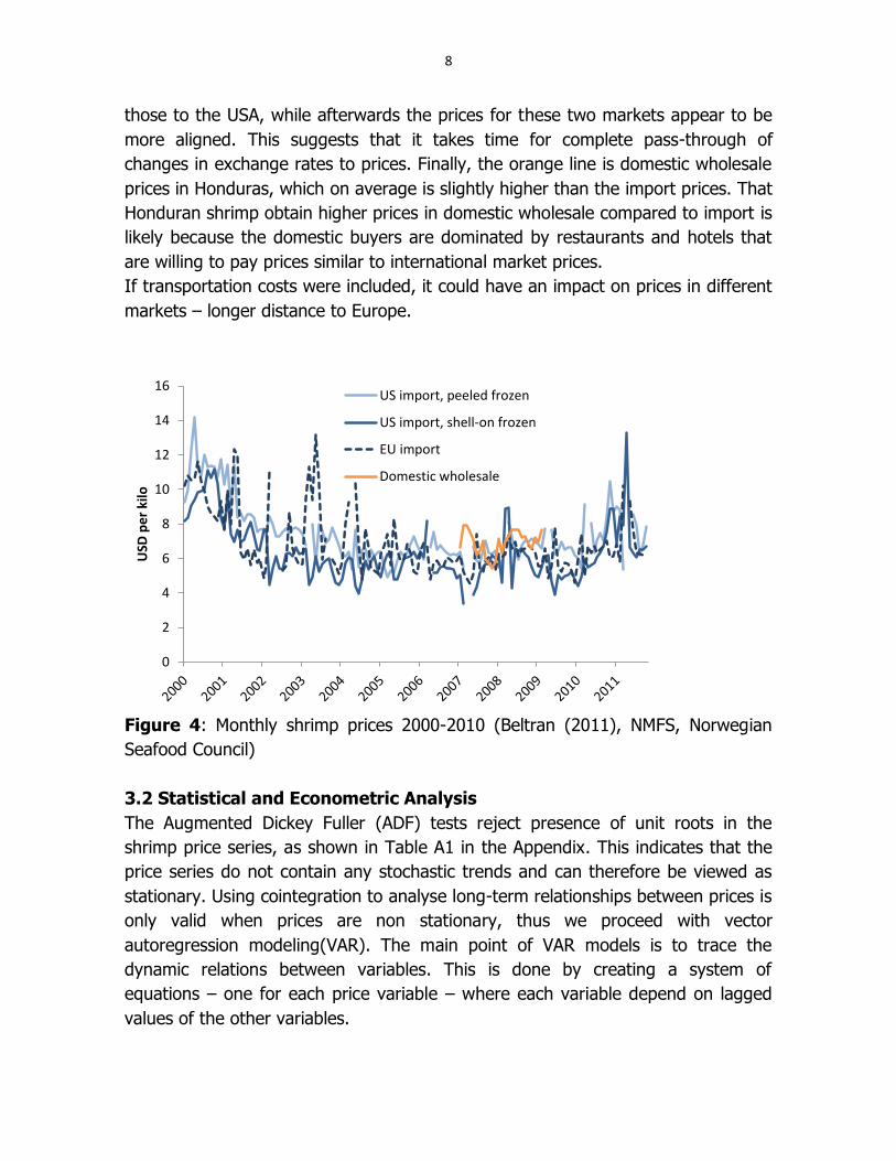
Figure 4 shows import prices paid for Honduran shrimp in different markets. These

prices support the supposition that exchange rates can have influenced relative

prices between USA and Europe. The dashed line is the import price to Europe for

frozen shrimp while the other two blue ones are for frozen whole and peeled to

the USA. From 2003 to 2005 average import price to Europe where higher than

0

2

4

6

8

10

12

14

2000 2001 2002 2003 2004 2005 2006 2007 2008 2009 2010

10

00

to

nn

es

USA

EU

8

those to the USA, while afterwards the prices for these two markets appear to be

more aligned. This suggests that it takes time for complete pass-through of

changes in exchange rates to prices. Finally, the orange line is domestic wholesale

prices in Honduras, which on average is slightly higher than the import prices. That

Honduran shrimp obtain higher prices in domestic wholesale compared to import is

likely because the domestic buyers are dominated by restaurants and hotels that

are willing to pay prices similar to international market prices.

If transportation costs were included, it could have an impact on prices in different

markets – longer distance to Europe.

Figure 4: Monthly shrimp prices 2000-2010 (Beltran (2011), NMFS, Norwegian

Seafood Council)

3.2 Statistical and Econometric Analysis

The Augmented Dickey Fuller (ADF) tests reject presence of unit roots in the

shrimp price series, as shown in Table A1 in the Appendix. This indicates that the

price series do not contain any stochastic trends and can therefore be viewed as

stationary. Using cointegration to analyse long-term relationships between prices is

only valid when prices are non stationary, thus we proceed with vector

autoregression modeling(VAR). The main point of VAR models is to trace the

dynamic relations between variables. This is done by creating a system of

equations – one for each price variable – where each variable depend on lagged

values of the other variables.

0

2

4

6

8

10

12

14

16

USD

per

kilo

US import, peeled frozen

US import, shell-on frozen

EU import

Domestic wholesale

9

According to the Aikake Information Criterion (AIC) one lag is sufficient for the

specification of the VAR model. Thus, one month lag contains most of the

predictive power in the model. The results from the estimated VAR model using

one month lag are shown in Table A2. In this model we used two variables, the

shell-on frozen shrimp to USA and frozen shrimp to EU. The estimated coefficients

indicate there is an interrelationship between the EU and US import prices of

Honduran shrimp. This is not unexpected as the shrimp market is known to be

integrated (Keithly and Poudel, 2008; Asche, Bennear, Oglend and Smith, 2011).

However, only the coefficient for the lagged US price influencing the EU price is

statistically significant and not vice versa when standard errors robust against

heteroscedasticity and autocorrelation are used. This suggests that the effect of

changes of US prices on EU prices is stronger than vice versa.

Figure 5 shows impulse response analysis based on a VAR model of frozen shrimp

prices to USA and EU. There is symmetry in the response of EU and USA prices on

each other as apparent from the diagrams in the upper-right and lower-left. The

effect of a change in EU price on the US price is somewhat stronger than vice

versa mainly because of stronger autocorrelation of US prices. For USA the

autocorrelation coefficient is 0.7 compared with 0.5 for EU (see estimation results

in table A2).

Figure 5: Impulse response analysis

0 5 10 15 20 25

0.25

0.50

0.75

1.00Lus_fz (Lus_fz eqn)

0 5 10 15 20 25

0.1

0.2

0.3 Leu_fz (Lus_fz eqn)

0 5 10 15 20 25

0.05

0.10

0.15Lus_fz (Leu_fz eqn)

0 5 10 15 20 25

0.25

0.50

0.75

1.00Leu_fz (Leu_fz eqn)

10

3.3 Comparison of traded and wholesale prices

Honduran wholesale prices are 20% higher than export prices to EU when

calculating the average shrimp prices during the period January 2007 to December

2008. The limited availability of domestic wholesale prices restricted the choice to

this period for comparison. As suggested above, the relatively high domestic prices

are due to buyers which compose mostly hotels and restaurants. However, the size

of these sectors limits the potential to increase sales in the domestic market. A

shift in the marketing from the international to the domestic market would require

a higher penetration of the consumer market. However, this would likely decrease

local market prices and it explains why producers export rather than market their

shrimp domestically.

3.4 Summary

The Honduran shrimp industry has grown rapidly and become a sizeable industry.

In value terms, shrimp is the most important seafood export product of Honduras.

The international marketplace for shrimp is highly competitive with large trade

flows coming from Asian countries to main markets such as USA and Europe. This

leads to harmonization of prices across geographical markets, something that is

also reflected in the econometric results when comparing the European and US

market for Honduran shrimp. The econometric model suggests that these prices

follow each other closely. However, the weakening of the USD relative to EUR

might explain why there was a considerable shift in the exports towards the

European market during the mid-2000s. The domestic wholesale prices are on par

or even higher than export prices. However, there are few domestic buyers willing

to pay comparable prices as the international market. In the case of small-scale

producers the local market can be a good alternative to international market.

4. ANALYSIS OF INTERNATIONAL TILAPIA VALUE CHAIN


Honduran tilapia is mainly destined as a fresh fillet product to the US market, as

shown from figure 6. It is also imported as frozen fillet, but at much lower volumes

than fresh fillet. From 2000 to 2008 US tilapia imports increased, but then fell in

2009 and grew slightly again in 2010.

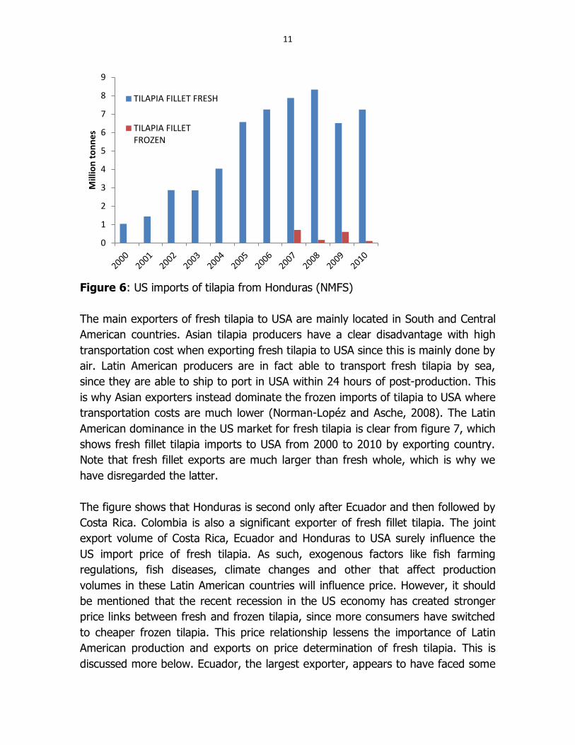
11

Figure 6: US imports of tilapia from Honduras (NMFS)

The main exporters of fresh tilapia to USA are mainly located in South and Central

American countries. Asian tilapia producers have a clear disadvantage with high

transportation cost when exporting fresh tilapia to USA since this is mainly done by

air. Latin American producers are in fact able to transport fresh tilapia by sea,

since they are able to ship to port in USA within 24 hours of post-production. This

is why Asian exporters instead dominate the frozen imports of tilapia to USA where

transportation costs are much lower (Norman-Lopéz and Asche, 2008). The Latin

American dominance in the US market for fresh tilapia is clear from figure 7, which

shows fresh fillet tilapia imports to USA from 2000 to 2010 by exporting country.

Note that fresh fillet exports are much larger than fresh whole, which is why we

have disregarded the latter.

The figure shows that Honduras is second only after Ecuador and then followed by

Costa Rica. Colombia is also a significant exporter of fresh fillet tilapia. The joint

export volume of Costa Rica, Ecuador and Honduras to USA surely influence the

US import price of fresh tilapia. As such, exogenous factors like fish farming

regulations, fish diseases, climate changes and other that affect production

volumes in these Latin American countries will influence price. However, it should

be mentioned that the recent recession in the US economy has created stronger

price links between fresh and frozen tilapia, since more consumers have switched

to cheaper frozen tilapia. This price relationship lessens the importance of Latin

American production and exports on price determination of fresh tilapia. This is

discussed more below. Ecuador, the largest exporter, appears to have faced some

0

1

2

3

4

5

6

7

8

9

Mill

ion

to

nn

es

TILAPIA FILLET FRESH

TILAPIA FILLETFROZEN

12

significant setbacks during the last years, as the US import volumes of Ecuadorian

fresh tilapia has decreased substantially since the peak year 2007. Hence, from

being the dominant source of fresh tilapia in the US market during the mid-2000s,

Ecuador is only slightly larger than Honduras in 2010 in terms of US import

volumes.

Figure 7: US imports of fresh fillet tilapia by country (NMFS)

Focusing on the fresh tilapia imports without taking into account the large volumes

of frozen tilapia that flows into the USA can be justified, since these products

appear to be separate market segments (Norman-Lopéz and Asche, 2008). These

findings suggest that consumers have different uses or preferences for these two

product formats. Therefore prices of frozen and fresh tilapia are not constrained to

follow a similar trend. This is shown partly in figure 8 that has domestic wholesale

prices together with import prices to USA for fresh and frozen fillets. The dark blue

graphs that represent frozen fillet prices do not follow the light blue of fresh fillet

prices. However, it should be said that the financial crisis of 2008 have made US

consumers more price sensitive, substituting fresh for lower-priced frozen tilapia

from Asia. Hence, the economic downturn may have strengthened price links

between fresh and frozen tilapia products. One result of this is that the US imports

of frozen tilapia have continued to grow, while fresh tilapia imports have

stagnated. However, here we will focus more on the competition between fellow

fresh tilapia exporters in Latin America, and as such leave frozen tilapia out of the

equation.

0

5

10

15

20

25

30

Mill

ion

to

nn

es

REST OF WORLD

EL SALVADOR

BRAZIL

COLOMBIA

COSTA RICA

HONDURAS

ECUADOR

13

Figure 8: Monthly domestic wholesale and USA import prices of Honduran tilapia

(Beltran (2011), NMFS)

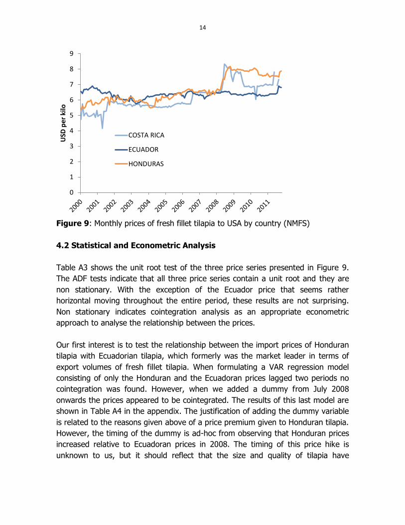
Since most of Honduran tilapia exports are fresh fillets to the USA, our analysis will

focus on the relationship with the main competitors in this specific market

segment. Figure 9 plots the US import prices of fresh tilapia fillets from Costa Rica,

Ecuador and Honduras. It is interesting to note that during 2008 both Costa Rican

and Honduran exporters experienced a price hike while the prices of Ecuadorian

tilapia remained more or less at a constant level. Then during the period from

2009 to 2011 Honduran tilapia, for most of the time, obtained higher prices

compared with its competitors in Ecuador and Costa Rica. This is interesting as it

suggests that fresh tilapia fillets from Costa Rica, Ecuador and Honduras are

imperfect substitutes. A likely explanation is the use of different production

technology used in Ecuador compared with Honduras and Costa Rica. The poly

culture of tilapia and shrimp together in Ecuador leads to harvesting of smaller

sized tilapia than in monoculture systems. The US market prefers the larger sized

tilapia fillets provided by Honduras, and the quality of tilapia meat from Honduras

has a high reputation.

0

1

2

3

4

5

6

7

8

9

USD

per

kilo

US import, fillets fresh

US import, fillet frozen

Domestic wholesale

14

Figure 9: Monthly prices of fresh fillet tilapia to USA by country (NMFS)


Table A3 shows the unit root test of the three price series presented in Figure 9.

The ADF tests indicate that all three price series contain a unit root and they are

non stationary. With the exception of the Ecuador price that seems rather

horizontal moving throughout the entire period, these results are not surprising.

Non stationary indicates cointegration analysis as an appropriate econometric

approach to analyse the relationship between the prices.

Our first interest is to test the relationship between the import prices of Honduran

tilapia with Ecuadorian tilapia, which formerly was the market leader in terms of

export volumes of fresh fillet tilapia. When formulating a VAR regression model

consisting of only the Honduran and the Ecuadoran prices lagged two periods no

cointegration was found. However, when we added a dummy from July 2008

onwards the prices appeared to be cointegrated. The results of this last model are

shown in Table A4 in the appendix. The justification of adding the dummy variable

is related to the reasons given above of a price premium given to Honduran tilapia.

However, the timing of the dummy is ad-hoc from observing that Honduran prices

increased relative to Ecuadoran prices in 2008. The timing of this price hike is

unknown to us, but it should reflect that the size and quality of tilapia have

0

1

2

3

4

5

6

7

8

9

USD

per

kilo

COSTA RICA

ECUADOR

HONDURAS

15

become important marketing factors. This is an interesting result as it gives room

for product differentiation.


From figure 8 it appears that US import prices of tilapia are higher that Honduran

wholesale prices. However, domestic prices likely refer to whole tilapia, in which

case price per kilo is lower than fillets. If we use a yield rate of 35% for fillets,

which appears to be reasonable, then the domestic price is in fact 11% higher

than the US import prices. This would suggest that local market prices can be

more lucrative than international trade prices. Generally, consumers in Honduras

have little tradition for seafood consumption, they prefer meat and chicken

(Beltrán, 2011). However, small-scale producers sell majority of their production in

the local market which is not sufficient to cover the domestic demand.

However, since large scale producers prefer to export tilapia fresh to USA, this

suggest that Honduran consumers are unwilling to pay a price premium for quality.

This is not surprising given the poor condition of marketing of fresh fish in

Honduras. Most Honduran consumers lack knowledge to determine freshness of

fish sold in either supermarkets or open markets, and they do not trust retailers to

provide top quality. Little have been done to ameliorate this situation in terms of

quality control, training and marketing of fish. The limited domestic market size

indicates that prices will fall if large volumes of tilapia are redirected from exports

to the domestic market. However, there is a clear growth potential of the domestic

market if the issues on how supermarkets and fish vendors fish market are

addressed. Such effort could provide a large payoff for small-scale producers of

tilapia and other species.

4.4 Summary

Honduras has become one of the leading exporters of fresh tilapia to USA, and in

value terms it is the largest. The high price that Honduran tilapia exporters receive

should reflect high quality standards in production. Exporters adhere to HAACP

standards and, moreover, there are standout tilapia producers in Honduras that

has receive certifications such as ISTRA standards (International Standards for

Responsible Tilapia Aquaculture) according to the WWF framework agreement and

GLOBAL GAP and other certificates. The main challenge that the industry faces in

international markets is competition from Asia combined with stagnating market

growth of fresh tilapia due to global economic recession. Fresh tilapia is a premium

16

product and consumer will tend to choose lower-priced alternatives such as frozen

tilapia in economic recessions. For small-scale producers the domestic market is an

alternative that can offer revenues as large as exporting. However, until the quality

control of fish marketed at the retail level is improved, the size of this market will

remain limited.

5. ANALYSIS OF INTERNATIONAL SPINY LOBSTER VALUE CHAIN


Spiny lobster harvesting is another important seafood industry in Honduras that is

export oriented. The lack of domestic prices for spiny lobster reflects that the

majority of the harvest is exported. The majority of international shipments are

destined for USA. Figure 10 shows total lobster imports to USA by exporting

country. The major exporter is neighbouring Canada followed by Brazil, Bahamas,

Nicaragua and Honduras. The Rest of World category is also large which reflects

that there are many countries that export lobster to USA.

Figure 10: US imports of lobster by country (NMFS)

In addition to the sizeable imports of lobster, USA also has a large lobster industry

of its own situated in New England. The Canadian and US harvest is dominated by

American lobster, of which spiny lobster species is not related. Spiny lobster (or

0

5

10

15

20

25

30

35

40

45

Mill

ion

to

nn

es

AUSTRALIA

HONDURAS

NICARAGUA

BAHAMAS

BRAZIL

CANADA

REST OF WORLD

17

rock lobster as it is more commonly known in food context) does not have claws

like American lobster. The tail contains the meat in spiny lobster, which is

considered coarser than American lobster but still known for a good flavour. In

Australia spiny lobster is known as crayfish, which further distinguishes it from true

lobster. Since the US imports from Canada are of American lobster, we will treat

this as a different market segment and concentrate on exporters of spiny lobster

from other Latin American countries.

However, the import prices of lobster from Canada are included in figure 11 along

with the four largest Latin American exporters to USA. Due to high volatility a

three-month moving average (3-MA) is used to better display long-term trends.

Even with a 3-MA there remains much short term variation in the series. However,

it is possible to observe similarities in long-term trends among the series. In

comparison to Honduras prices, the most similar appear to be Bahamas and

Nicaragua. Differences in species types can explain why US import prices of

Canadian lobster follow somewhat different cycles than the Latin American

countries. Brazil, however, harvests mainly Caribbean spiny lobster like the other

Latin American countries. Nevertheless import prices of lobster from Brazil show

strong short-term deviations in price movements from the other prices. This

suggests that different seasonal pattern in spiny lobster harvesting among

exporting countries can make it difficult for US importers to shift suppliers, at least

during certain periods of the year. It should be mentioned that US import statistics

do not distinguish between product formats. For example, spiny lobster is traded

as entire, tails and meat and this implies that the import price can be influenced by

the composition of the imports. In the following analysis we will concentrate more

on the Bahamas, Honduras and Nicaragua which prices appear to be closely

integrated. The three price series are presented in Figure 12.

18

Figure 11: US lobster import prices as 3-months moving average by the five

largest exporting countries (NMFS)

Figure 12: US lobster import prices as 3-months moving average by Bahamas,

Honduras and Nicaragua (NMFS)

0

5

10

15

20

25

30

35

40

45

50

BAHAMAS

BRAZIL

CANADA

HONDURAS

NICARAGUA

0

5

10

15

20

25

30

35

40

45

50

BAHAMAS

HONDURAS

NICARAGUA

19


Following the same econometric approach as the prior two case studies, we start

with unit root tests of price series. The series analysed are the five prices

presented in figure 11, i.e., US import prices of lobster from Bahamas, Brazil,

Canada, Honduras and Nicaragua. The results of the ADF tests of the five price

series are reported in Table A5 in the Appendix. The null of nonstationarity is

rejected for the first difference of the logarithmic prices for all five cases, which is

as expected. When the ADF tests are run on the levels of the logarithmic

transformed prices the hypothesis of nonstationarity is also rejected for most of

the price series. This suggests that the price series are stationary or near-

stationary in which case cointegration is not an appropriate tool of analysis.

Instead we formulate a VAR models using the five series.

Above we indicated that the lobster prices originating from Honduras, Nicaragua

and Bahamas appeared more tightly integrated by visual inspection of figure 11

and 12. A VAR analysis allows us to test this hypothesis by examining the dynamic

relationship between the prices. The first VAR model included all five price series.

This model confirmed our suspicion that the import prices of Canadian and Brazil

do not seem to be directly related to Central American and Caribbean prices. As a

result, we re-specify the model to only include prices from Central America and

Caribbean i.e. Bahamas, Honduras and Nicaragua. The estimation results of this

VAR model specification are presented in table A6. From the results, it is

interesting to note that Honduran prices seem to have more short-run impact on

the Bahaman and Nicaraguan prices in the short run than vice versa.

However, an impact response analysis can give additional information on the long-

term impact of changes of one price on another. Figure 13 presents the cumulative

impulse responses for the three equations. The top three diagrams represent

impulse responses for the Bahaman prices followed by the middle row for the

Honduran prices and the bottom row for Nicaraguan prices. If we concentrate on

the middle row for Honduras, it appears that Bahaman prices have a stronger

influence on Honduran prices than Nicaraguan. The larger volumes of imported

lobster originating from Bahamas compared to Nicaragua can explain its greater

influence on price formation.

20

Figure 13: Cumulative impulse response analysis

5.3 Summary

Honduran lobster, which is a product mainly destined for exports due to its

exclusivity, face competition from a number of other exporting countries. Although

Honduras belongs among the top five exporters of lobster to USA in volume terms,

it still accounts for a relatively small share of total lobster imports to the USA,

which is made up of different species. Domestic sales are mainly directed to

restaurants and upscale hotels as this is an exclusive product. This can explain why

domestic wholesale prices are not available. Even if the domestic market is small,

the exclusivity of the product can make lobster harvesting a profitable endeavour

for small-scale fishers.

6. ANALYSIS OF INTERNATIONAL SNAPPER VALUE CHAIN


The largest fisheries in Honduras are marine fishes, shrimp, stromboid conch, and

spiny lobster. Snapper and grouper make up the largest portion of the marine fish

category, in particular the former accounts for a large share. The industrial

fisheries of red snapper are export-oriented where most fish are shipped fresh

whole to the USA. Figure 14 shows US import prices of red snapper from Honduras

together with domestic wholesale prices. The figure shows that until 2009 there

was only a very weak increasing trend, while after 2009 prices have increased

0 20 40

1.5

2.0

cum Lbahamas (Lbahamas eqn)

0 20 40

0.25

0.50

0.75

1.00cum Lhonduras (Lbahamas eqn)

0 20 40

0.00

0.25

cum Lnicaragua (Lbahamas eqn)

0 20 40

0.5

1.0

1.5cum Lbahamas (Lhonduras eqn)

0 20 40

1.5

2.0cum Lhonduras (Lhonduras eqn)

0 20 40

0.00

0.25

0.50

0.75cum Lnicaragua (Lhonduras eqn)

0 20 40

1

2cum Lbahamas (Lnicaragua eqn)

0 20 40

0.5

1.0

1.5cum Lhonduras (Lnicaragua eqn)

0 20 40

2

3

cum Lnicaragua (Lnicaragua eqn)

21

rapidly. There is also a relatively high volatility in the prices influenced by

seasonality in the catches.

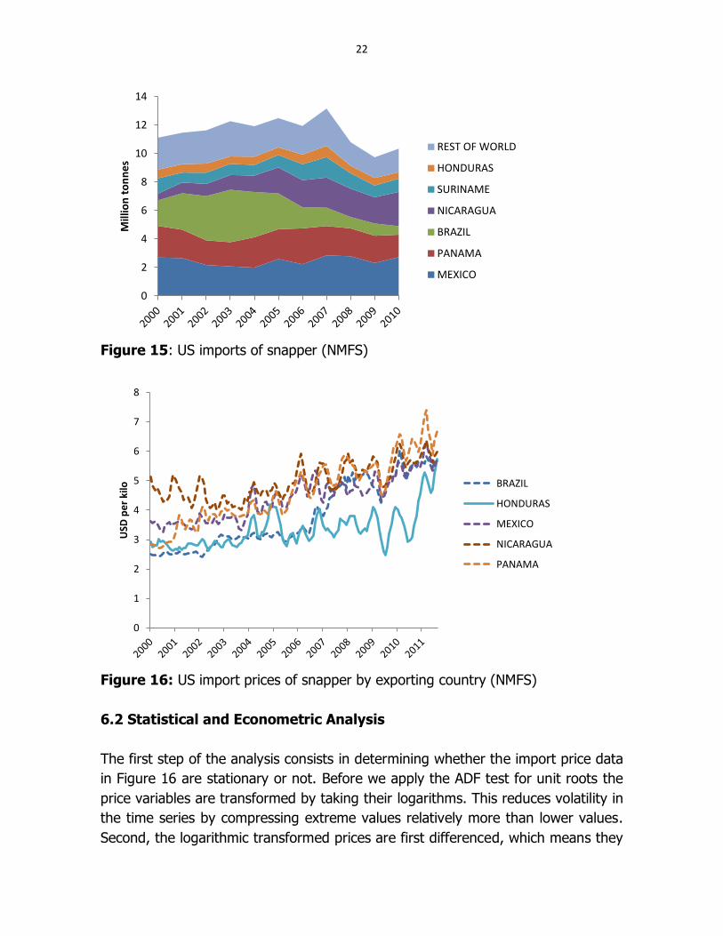
There are several countries besides Honduras that export snapper to USA as

shown in Figure 15. In the early 2000s Brazil, Mexico and Panama were the largest

exporters to USA, but during the last five years Nicaragua has grown to be the

second largest after Mexico. Countries export different snapper species, which

makes this market less commodified than say shrimp and lobster. The

heterogeneity of species, product format and size in imports of snapper to USA

makes it less obvious how import prices of red snapper from Honduras is

influenced by other US snapper imports. Figure 16 shows that most of the snapper

import prices have an increasing trend during the data period. However, the

steepness of the trend differs between the series and also the short term volatility

differs. The relationship between these prices will be analysed in the following

section.

Figure 14: US import prices and domestic wholesale prices of Red snapper

(Beltran (2011), NMFS)

0

1

2

3

4

5

6

7

USD

pe

r ki

lo

US import

Domestic wholesale

22

Figure 15: US imports of snapper (NMFS)

Figure 16: US import prices of snapper by exporting country (NMFS)


The first step of the analysis consists in determining whether the import price data

in Figure 16 are stationary or not. Before we apply the ADF test for unit roots the

price variables are transformed by taking their logarithms. This reduces volatility in

the time series by compressing extreme values relatively more than lower values.

Second, the logarithmic transformed prices are first differenced, which means they

0

2

4

6

8

10

12

14

Mill

ion

to

nn

es

REST OF WORLD

HONDURAS

SURINAME

NICARAGUA

BRAZIL

PANAMA

MEXICO

0

1

2

3

4

5

6

7

8

USD

pe

r ki

lo BRAZIL

HONDURAS

MEXICO

NICARAGUA

PANAMA

23

reflect the changes in prices from period to period rather than the price level. The

first five unit root tests in table A7 in the appendix are of the first difference of the

logarithmic price variables. As expected the hypothesis of nonstationarity is

rejected for all five series, which implies that the price series do not contain two or

more unit roots. Next we apply unit root test at the levels of the logarithmic prices,

which is now a test of whether the series contain one unit root. Brazil, Honduras

and Panama appear to contain a unit root, while Nicaragua and Mexico do not

contain when the ADF test is evaluated at the lowest AIC value. However, when

we add a trend to the ADF test most of the series appear to be trend stationary,

i.e., normally distributed around a deterministic trend.

By taking the first differencing of the log price variables implies that the trends in

the series are removed. Thus, we will analyse the price variables using the first

difference of the logarithms. The next step is formulating VAR models using the

five transformed price series. Each model will contain the US import prices of

Honduran snapper. After estimating several models with different combinations of

the price series, it becomes clear that the price linkages between Honduran

snapper and snapper from other countries are weak with exception of Panama. In

a VAR model that contain only import prices of Honduran and Panamanian

snapper, there seems to be a little effect of import prices of Honduran snapper on

Panamanian snapper. This is confirmed by applying a Granger causality test, which

fail to reject the hypothesis that price of Honduran snapper influences the import

price of Panamanian snapper. Thus, we reduce the VAR system to a single

equation model for the import price of Honduran snapper. The results of this final

model are presented in Table A8 in the Appendix. With two lags for the own prices

and the Panamanian price the model appears to be well specified. The most

important result is that a 1% increase in the price of Panamanian snapper leads to

a 0.72% increase in the price of Honduran snapper.

From figure 16 it is apparent that the import price of Honduran snapper has lagged

behind the price increase of the large exporters of snapper to USA. However, the

catching up during 2010-11 signal that these markets are not entirely separated.

The findings from the econometric model suggest that Honduran exports to USA

are influenced by Panamanian snapper exports in the long run. Given that total

import volume of snapper to USA have stagnated during the last years and if this

reduction is related to lower landings of snapper due to biological constraints of

wild snapper stocks, prices are likely to remain firm.

24


When comparing average prices of Honduran snapper in the US import market and

wholesale in Honduras from the period when domestic prices are available, we

found that import prices are 11% higher than domestic wholesale prices.

Transportation costs are likely substantial for the exports to the USA, as it is

exported fresh. This can explain some of the price differentiation. In addition, most

of limitations of the domestic market of tilapia also apply here. Lacking quality

control and marketing of fish products in Honduras limits the size of the domestic

market and can explain why a majority of snapper fish is exported.

6.4 Summary

Snapper is an important species in Honduran fisheries where a large share is

exported to USA fresh. Honduran snapper competes with snapper from several

other Latin American countries. However, the econometric analysis indicated that

the price linkages are weak among some of the trade flows of snapper to the USA,

suggesting that there is heterogeneity in species, quality and product format of

imports. Panamanian exports of snapper to USA seems to exert the strongest

influence on Honduran snapper exports, while Brazil, Mexico and Nicaragua do not

appear to influence Honduran prices much, despite the importance of those three

countries in the US snapper market. Snapper is another seafood product where

small-scale fishers have a lot to gain from improved marketing and infrastructure

for distribution of fish in Honduras.

7. SUMMARY AND CONCLUDING DISCUSSION

This report has analysed prices of some of Honduras most important seafood

products – shrimp, tilapia, spiny lobster and snapper. The objective of the study is

to shed light on how Honduran fishers and fish farmers, especially small scale

producers, can improve their livelihoods by participating in value chains that pay

higher prices for their fish. To fulfil this objective we analyse price formation in

domestic and international value chains where the Honduran seafood industry

participates.

25

A large share of the Honduran seafood production is exported to USA. This means

that seafood producers in Honduras participate directly in competitive and

demanding international markets. It can be useful to reflect on what this implies

for price determination of fish products. Globally, seafood is traded more than any

agricultural product as a share of 39% of global seafood is shipped internationally

(Food and Agricultural Organization of the United Nations, 2010). Comparing

seafood trade-to-consumption in individual countries allows us to estimate

exposure to competition in seafood markets. Tveteras et al. (2012) estimated that

78% of global seafood production is exposed to trade competition. Honduras has a

seafood trade-to-consumption ratio of 1.75. This means that in Honduras the level

of seafood imports plus exports are 175% higher than the domestic seafood

consumption. The high ratio implies that not only traded Honduran fish is exposed

to international competition, but also non-traded fish that could also have been

exported. In other words, if we analyse prices of exported fish from Honduras, this

will also have bearing on price formation domestically of the same products.

Also note that an individual exporter’s influence on prices in international seafood

markets relies on its size and the type of demand the exporter faces. Honduran

seafood producers, which are relatively small in an international context, are likely

to have limited influence on fish prices. The only exception could be if Honduran

seafood exporters dominate some market niche or segment for a product with few

substitutes. This is an issue we will explore further.

In international trade of shrimp many exporting countries compete. When

competition is strong price movements tend to be aligned across geographical

markets. Accordingly, the analysis in report shows that import price of Honduran

shrimp is very similar in EU and USA, indicating that these two markets are

integrated. Moreover, a couple of other studies have shown that the US shrimp

market is highly competitive (Asche et al 2011a; Keithly and Poudel, 2008).

Despite not influencing international prices, Honduran exporters can still choose

where to sell their shrimp. During the data period, the flow of Honduran shrimp

exports has shifted back and forth between the EU and the US market. Changes in

USD/EUR exchange rate have changed relative prices between these two markets

and thereby created profitable opportunities of shifting market. Thus even if a

shrimp producer do not have market power, higher revenues can be obtained by

being flexible in terms of product processing and marketing. This requires the

ability to monitor markets and to have sufficient processing and marketing

capabilities to be able to deliver exactly what the market demands.

26

Tilapia is other seafood where price are mostly determined in international markets

(Norman-Lopez and Asche, 2008; Norman-Lopez and Bjørndal, 2009). In the US

market, Asian producers dominate the frozen tilapia segment, while Latin American

producers dominate the fresh tilapia segment. When measured in import value,

Honduras is in fact the largest exporters of fresh tilapia to USA followed by

Ecuador and Costa Rica as the main competitors in the fresh tilapia market. Total

imports of fresh tilapia have stagnated to USA, a trend that has been linked to the

global economic recession. Fresh tilapia is a more exclusive product and many

consumers have shifted towards cheaper frozen tilapia. While import prices of

fresh tilapia sourced from different countries tend to follow the same price trend

there are some divergence in the price movements. Figure 9 shows that the price

level for Honduran tilapia increased significantly in 2009, while Ecuadorian tilapia

has remained on a lower price level. The most likely explanation is that Honduran

producers have better control with the production process, because they use

monoculture production systems instead of polyculture system used in Ecuador.

Better control allows optimization of fish size and production of higher quality fish

meat. This suggests that there are opportunities for product differentiation in the

tilapia market.

While Honduran shrimp and tilapia exports mainly derive from aquaculture, spiny

lobster is a capture fishery product. This is an exclusive product where domestic

buyers are high-end restaurants and hotels. However, the larger market is the

export market. As with shrimp and tilapia, most exports are directed to USA. In

this market spiny lobster faces competition both with domestic lobster and with

imported lobster from many other countries. Figure 10 and 11 show that the

import volume and prices of lobster to USA. The total import volume has remained

relative constant during the 10-year period although with a slight increase in 2010.

However, after import prices peaked around 2008 there was a sharp downward

correction in 2009.

The US market for lobsters is dominated by two different types of lobster,

American lobsters, which is produced domestically and imported from Canada, and

spiny lobster (also known as rock lobster) that is widely imported from Latin

American and Caribbean countries. Thus, while it is obvious from Figure 11 that

there are some common long-term price trends, it seems that short term price

variation of Honduran spiny lobster exports are more influenced by Bahaman and

Nicaraguan spiny lobster imports, rather than say US imports of Canadian lobster.

27

Finally, the last case studies analyses US import prices of snapper from Honduras.

Like spiny lobster, snapper is fisheries product that faces competition from several

other Latin American countries that export snapper to USA. Importantly, the

analyses show that US import prices of snapper from Panama appears to have a

bearing on Honduran prices. However, snapper seems to be a much more

fragmented market than, say, shrimp probably owing to the diversity of snapper

species, quality and product format and size. The fact that it is a fishery product

means there is less control with production volume and size of individual fish

caught. Heterogeneity of the imported snapper is thus one important explanation

for some of the price trends. Interestingly, US import prices of Honduran snapper

have been lagging behind the price increases observed for snapper from other

countries. This indicates that marketing of Honduran snapper could be improved.

The above discussion has concentrated on the international value chains for

Honduran seafood. However, one of the main points in the report is the potential

to improve the domestic marketing of fish. Poor infrastructure, lack of trust

between buyer and seller, variable product quality are some of the factors that

undermine the potential of the domestic market. Local supermarkets are known to

have sub-optimal storage of fish, so that it loses freshness. Also, there is little if

any effort to market fish for domestic consumption which points to a huge

potential to boost domestic consumption of fish. As of now, fish sold domestically

are influenced by export prices, especially for those species that are widely

exported. But the size of the local market is constrained by the factors mentioned

above. This is a hurdle for small-scale producers who often lack the resources

required to access export markets. The end result is that local market prices will be

depressed compared to export prices. This is not evident from the domestic

wholesale prices reported here, but the question remains how representative they

are for the average small scale producer.

For aquaculture another important growth factors are availability of land and water

resources suitable for farming shrimp and tilapia, credit and skilled labour. Land

resource constraints could be solved by intensifying aquaculture production. For

example, Asian shrimp producers have gradually shifted towards more intensive

production system. In contrast, semi-intensive production systems dominate Latin

American shrimp aquaculture. This is also the case for Honduran shrimp

aquaculture (Valderrama and Engle 2001). However, such a move requires capital

and know-how both of which tend to be scarce. Few if any banks are willing to

provide credits for aquaculture investments as this business sector is perceived as

high risk. Semi-intensive systems have advantages in terms of lower production

28

risk and are believed to produce more tasty meat - an important quality for fresh

product marketing. For now, the shrimp industry is aware of the risks associated

with rapid expansion and how chosen a cautious growth strategy (Valderrama,

2012). This appears to be a wise choice given experiences with disease outbreaks

and the subsequent need of strong control of the production environment.

Exporters of fresh tilapia to USA have been facing weaker market demand, since

the total import volume of peaked in 2007-08. Honduran exporters have been

holding up well, however, and have also been able to extract premium prices

compared to some of its competitors. This suggests that degree of professionalism

in the Honduran tilapia industry has made room for further expansion. The growth

of Caribbean and Latin American economies opens up new marketing opportunities

for Honduran seafood products. In this respect, maintaining high quality standards

is important. Moreover, tourism is another industry that can support the seafood

industry through increased consumption of seafood in Honduras, but also through

activities directly related to seafood. This could particularly be an option in fisheries

where growth is constrained by the natural productivity of the fishing grounds. As

a result, sustainable and efficient use of resources together with more value added

productions are keys for the Honduran seafood industry to keep growing and

creating new livelihoods. This suggests that small scale producers need continued

access to training and credit to keep up with the standards of demanding

international markets.

29

8. REFERENCES Asche, F., Bennear, L. Bennear, A. Oglend, and M.D. Smith. (2011a). U.S. Shrimp Market Integration (November 1, 2011). Duke University Environmental Economics

Working Paper No. EE-11-09. Asche, F. and Bjørndal, T. (2011). The Economics of Salmon Aquaculture, Second

Edition, Wiley-Blackwell, Oxford, UK

Asche, F., A. Oglend, and S. Tveteras. (2011b). Regime Shifts in the Fish Meal/Soyabean Meal Price Ratio, unpublished working paper.

Asche, F. and S. Tveterås (2004). “On the Relationship between Aquaculture and Reduction Fisheries.” Journal of Agricultural Economics, 55(2): 245-265.

Asche, F., H. Bremnes, and C. R. Wessells (1999) "Product Aggregation, Market Integration and Relationships Between Prices: An Application to World Salmon Markets", American Journal of Agricultural Economics, 81, 568-581.

Asche, F., K. G. Salvanes, and F. Steen (1997) "Market Delineation and Demand Structure", American Journal of Agricultural Economics, 79, 139-150.

Asche, F., and T. Sebulonsen (1998) "Salmon Prices in France and the UK: Does Origin or Market Place Matter?", Aquaculture Economics and Management, 2, 21-

30.

C. Beltrán (2011). Value-chain analysis of international fish trade and food security in the Republic of Honduras. (February, 2011) Food and Agricultural Organization of the united Nations.

Cheung, Y. and Lai, K. 1993. Finite Sample Sizes of Johansen’s Likelihood Ratio Tests for Cointegration. Oxford Bulletin of Economics and Statistics, 55:313-328.

Cournot, A. A. (1971) Researches into the Mathematical Principles of the Theory of Wealth, A. M. Kelly, New York.

Drakeford, B. and S. Pascoe (2008). “Substitutability of fishmeal and fish oil in diets for salmon and trout: A meta-analysis,” Aquaculture Economics &

Management, 12(3): 155-175. Engle, R. F., and C. W. J. Granger (1987) "Co-integration and Error Correction:

Representation, Estimation and Testing", Econometrica, 55, 251-276.

30

Food and Agricultural Organization of the United Nations (2010). The State of World Fisheries and Aquaculture 2010. Rome: Food and Agricultural Organization of the United Nations.

Fréon, P., Bouchon, M., Domalain, G., Estrella, C, Iriarte, F., Lazard, J., Legendre M., Quispe, I., Mendo, T., Moreau, Y., Nuñez, J., Sueiro, J.C., Tam, J., Tyedmers,

P., and Voisin, S. (2010). Impacts of the Peruvian anchoveta supply chains: from wild fish in the water to protein on the plate. GLOBEC International Newsletter, April 2010 16(1): 27-31

Goodwin, B. K., T. J. Grennes, and M. K. Wohlgenant (1990) "A Revised Test of the Law of One Price Using Rational Price Expectations", American Journal of Agricultural Economics, 72, 682-693. Gordon, D. V., K. G. Salvanes, and F. Atkins (1993) "A Fish Is a Fish Is a Fish:

Testing for Market Linkage on the Paris Fish Market", Marine Resource Economics, 8, 331-343.

Johansen, S. (1988) "Statistical Analysis of Cointegration Vectors", Journal of Economic Dynamics and Control, 12, 231-254.

Johansen, S., and K. Juselius (1990) "Maximum Likelihood Estimation and Inference on Cointegration - with Applications to the Demand for Money", Oxford Bulletin of Economics and Statistics, 52, 169-210. Johansen, S., and K. Juselius (1992) "Testing Structural Hypothesis in a

Multivariate Cointegration Analysis of the PPP and the UIP for UK", Journal of Econometrics, 53, 211-244.

Keithly Jr., W.R. and P. Poudel. 2008. The Southeast U.S.A. Shrimp Industry: Issues Related to Trade and Antidumping Duties. Marine Resource Economics 23(4):439-63.

Kristofersson, D. and J, L. Anderson (2005). “Is there a relationship between fisheries and farming? Interdependence of fisheries, animal production and

aquaculture.” Marine Policy 30(6): 721-725. Lewbel, A. (1996) "Aggregation without Separability: A Generalized Composite

Commodity Theorem", American Economic Review, 86, 524-561. Nielsen, M., J. Setala, J. Laitinen, K. Saarni, J. Virtanen and A. Honkanen (2007).

Market Integration of Farmed Trout in Germany. Marine Resource Economics, 22(2), 195-213.

31

Nordahl, P. G. (2011). Is the fishmeal industry caught in a fishmeal trap. Master

thesis. Norway, Bergen: Norwegian School of Economics (NHH). Norman-Lopez, A. and F. Asche. (2008). "Competition Between Imported Tilapia

and US Catfish in the US Market," Marine Resource Economics 23(2), 199-214.

Norman-Lopez, A. and T. Bjørndal. (2009). “Is Tilapia the Same Product Worldwide or Are Markets Segmented?” Aquaculture Economics and Management, 13(2): 138-154.

Ravallion, M. (1986) "Testing Market Integration", American Journal of Agricultural Economics, 68, 102-109.

Stigler, G. J., and R. A. Sherwin (1985) "The Extent of a Market", Journal of Law and Economics, 28, 555-585.

Tveteras, S. (2010). “Forecasting with Two Price Regimes: A Markov-Switching VAR Model for Fish Meal Price,” Journal of Centrum Catedra, 3(1), 34-40, 2010.

Tveteras, S. and R., Tveteras. (2010). “The Global Competition for Wild Fish Resources between Livestock and Aquaculture.” Journal of Agricultural Economics.

61(2), 381-397.

Tveteras, S., F. Asche, M. F. Bellemare, M. D. Smith, A. G. Guttormsen, A. Lem, K. Lien, S. Vannuccini. (2012). Fish Is Food - The FAO’s Fish Price Index. Unpublished manuscript.

Valderrama, D. and C. Engle. “Risk Analysis of Shrimp Farming in Honduras.” Aquaculture Economics and Management, 5(1): 49-68.

Valderrama, D. (2012). Personal communication through email.

32

9. APPENDIX

Table A1. Unit root tests of EU and US import prices of frozen shrimp, Jan 2000 –Sep 2011 Unit-root tests (using Shrimphonduras)

The sample is 2000 (6) - 2011 (9)

DLus_peelfz: ADF tests (T=136, Constant; 5%=-2.88 1%=-3.48)

D-lag t-adf beta Y_1 sigma t-DY_lag t-prob AIC F-prob

3 -9.589** -1.4249 0.1153 2.745 0.0069 -4.285

2 -10.02** -0.97431 0.1181 2.509 0.0133 -4.244 0.0069

1 -11.47** -0.62318 0.1204 2.089 0.0387 -4.212 0.0012

0 -17.40** -0.37690 0.1219 -4.195 0.0005

DLus_fz: ADF tests (T=136, Constant; 5%=-2.88 1%=-3.48)


3 -8.194** -1.0727 0.1623 0.9623 0.3377 -3.600

2 -10.00** -0.91351 0.1623 1.827 0.0700 -3.608 0.3377

1 -12.76** -0.65464 0.1637 3.946 0.0001 -3.598 0.1229

0 -14.95** -0.25007 0.1724 -3.502 0.0003

DLeu_fz: ADF tests (T=136, Constant; 5%=-2.88 1%=-3.48)


3 -8.333** -1.0064 0.1971 2.109 0.0369 -3.212

2 -8.809** -0.69415 0.1996 0.6462 0.5193 -3.194 0.0369

1 -12.17** -0.60382 0.1992 3.345 0.0011 -3.205 0.0913

0 -15.03** -0.25469 0.2066 -3.139 0.0015

Lus_peelfz: ADF tests (T=136, Constant; 5%=-2.88 1%=-3.48)


3 -3.027* 0.83246 0.1146 -2.088 0.0388 -4.297

2 -3.347* 0.81464 0.1160 -1.585 0.1153 -4.279 0.0388

1 -3.638** 0.80016 0.1167 -3.744 0.0003 -4.275 0.0341

0 -4.674** 0.74202 0.1222 -4.189 0.0002

Lus_fz: ADF tests (T=136, Constant; 5%=-2.88 1%=-3.48)


3 -2.787 0.82287 0.1583 -1.269 0.2067 -3.651

2 -3.102* 0.80652 0.1586 -3.035 0.0029 -3.653 0.2067

1 -4.000** 0.75329 0.1635 -1.563 0.1203 -3.600 0.0054

0 -4.822** 0.71972 0.1643 -3.597 0.0049

Leu_fz: ADF tests (T=136, Constant; 5%=-2.88 1%=-3.48)


3 -4.464** 0.61140 0.1867 0.6072 0.5448 -3.321

2 -4.487** 0.62643 0.1862 -1.647 0.1019 -3.332 0.5448

1 -5.462** 0.57532 0.1874 -0.5920 0.5548 -3.327 0.2195

0 -6.403** 0.55491 0.1870 -3.339 0.3352

Table A2. VAR model of EU and US import prices of frozen shrimp, Jan 2000 –Sep 2011 SYS(10) Estimating the system by OLS (using Shrimphonduras)

The estimation sample is: 2000 (2) to 2011 (9)

URF equation for: Lus_fz

Coefficient Std.Error HACSE t-HACSE t-prob

Lus_fz_1 0.695157 0.06154 0.08724 7.97 0.000

Leu_fz_1 0.121542 0.06326 0.07706 1.58 0.117

33

Constant U 0.318444 0.1245 0.1687 1.89 0.061

sigma = 0.162337 RSS = 3.61042439

URF equation for: Leu_fz


Lus_fz_1 0.258742 0.06822 0.07547 3.43 0.001

Leu_fz_1 0.495461 0.07012 0.09119 5.43 0.000

Constant U 0.487848 0.1380 0.1141 4.28 0.000

sigma = 0.179949 RSS = 4.436262726

log-likelihood 100.402001 -T/2log|Omega| 497.70479

|Omega| 0.000816839096 log|Y'Y/T| -5.87535026

R^2(LR) 0.709083 R^2(LM) 0.404603

no. of observations 140 no. of parameters 6

F-test on regressors except unrestricted: F(4,272) = 58.0737 [0.0000] **

F-tests on retained regressors, F(2,136) =

Lus_fz_1 69.6294 [0.000]** Leu_fz_1 26.3456 [0.000]**

Constant U 9.26612 [0.000]**

correlation of URF residuals (standard deviations on diagonal)

Lus_fz Leu_fz

Lus_fz 0.16234 0.020521

Leu_fz 0.020521 0.17995

correlation between actual and fitted

Lus_fz Leu_fz

0.75720 0.66269

Lus_fz : Portmanteau(12): 17.5133

Leu_fz : Portmanteau(12): 15.6224

Lus_fz : AR 1-7 test: F(7,130) = 1.5863 [0.1449]

Leu_fz : AR 1-7 test: F(7,130) = 0.60687 [0.7494]

Lus_fz : Normality test: Chi^2(2) = 43.444 [0.0000]**

Leu_fz : Normality test: Chi^2(2) = 12.381 [0.0020]**

Lus_fz : ARCH 1-7 test: F(7,123) = 1.6679 [0.1230]

Leu_fz : ARCH 1-7 test: F(7,123) = 1.1850 [0.3163]

Lus_fz : hetero test: F(4,132) = 2.2493 [0.0671]

Leu_fz : hetero test: F(4,132) = 1.1704 [0.3268]

Lus_fz : hetero-X test: F(5,131) = 1.8048 [0.1162]

Leu_fz : hetero-X test: F(5,131) = 1.9834 [0.0852]

Vector Portmanteau(12): 52.9053

Vector AR 1-7 test: F(28,244)= 1.0142 [0.4504]

Vector Normality test: Chi^2(4) = 55.713 [0.0000]**

Vector hetero test: F(12,344)= 1.2670 [0.2364]

Vector hetero-X test: F(15,356)= 1.4384 [0.1267]

Table A3. Unit root tests of US import prices of fresh fillet tilapia, Jan 2000 – Sep 2011 Unit-root tests (using Tilapiahonduras)

The sample is 2000 (6) - 2011 (10)

DLcostarica: ADF tests (T=137, Constant; 5%=-2.88 1%=-3.48)


3 -6.632** -0.40633 0.03978 1.537 0.1266 -6.413

2 -6.750** -0.24170 0.03999 -1.945 0.0539 -6.410 0.1266

1 -10.84** -0.48374 0.04040 1.768 0.0793 -6.396 0.0487

0 -15.65** -0.28961 0.04072 -6.388 0.0277

DLecuador: ADF tests (T=137, Constant; 5%=-2.88 1%=-3.48)

34


3 -5.970** -0.21462 0.01496 0.9443 0.3468 -8.369

2 -6.435** -0.11374 0.01495 -1.506 0.1346 -8.377 0.3468

1 -9.666** -0.28220 0.01502 0.9581 0.3397 -8.374 0.2102

0 -14.00** -0.18429 0.01502 -8.382 0.2576

DLhonduras: ADF tests (T=137, Constant; 5%=-2.88 1%=-3.48)


3 -5.035** 0.0055789 0.02320 -1.484 0.1401 -7.492

2 -6.602** -0.13910 0.02330 -0.9452 0.3463 -7.490 0.1401

1 -9.230** -0.24123 0.02329 0.1172 0.9069 -7.498 0.2156

0 -14.79** -0.22887 0.02321 -7.512 0.3774

Lcostarica: ADF tests (T=137, Constant; 5%=-2.88 1%=-3.48)


3 -1.489 0.96061 0.03980 2.112 0.0366 -6.412

2 -1.239 0.96702 0.04032 -1.624 0.1068 -6.393 0.0366

1 -1.419 0.96224 0.04056 -3.258 0.0014 -6.388 0.0305

0 -1.896 0.94844 0.04198 -6.326 0.0007

Lecuador: ADF tests (T=137, Constant; 5%=-2.88 1%=-3.48)


3 -2.197 0.91191 0.01474 1.905 0.0589 -8.398

2 -1.860 0.92596 0.01489 -0.5182 0.6052 -8.386 0.0589

1 -2.037 0.92127 0.01485 -1.627 0.1061 -8.398 0.1461

0 -2.507 0.90559 0.01494 -8.393 0.0915

Lhonduras: ADF tests (T=137, Constant; 5%=-2.88 1%=-3.48)


3 -0.7870 0.98652 0.02334 0.9941 0.3220 -7.480

2 -0.7224 0.98765 0.02334 -0.07732 0.9385 -7.487 0.3220

1 -0.7305 0.98758 0.02325 -2.662 0.0087 -7.501 0.6094

0 -0.9815 0.98302 0.02377 -7.464 0.0498

Table A4. VAR model of US import prices of fresh fillet tilapia from Honduras and

Ecuador, Jan 2002 – Sep 2011 SYS(22) Estimating the system by OLS (using Tilapiahonduras)


URF equation for: Lecuador


Lecuador_1 0.776922 0.09067 0.1038 7.49 0.000

Lecuador_2 0.120090 0.09787 0.1074 1.12 0.266

Lhonduras_1 0.133093 0.06652 0.07738 1.72 0.088

Lhonduras_2 -0.137021 0.06330 0.06831 -2.01 0.047

d2008 0.00396951 0.007466 0.007669 0.518 0.606

Constant U 0.196167 0.09335 0.07838 2.50 0.014

sigma = 0.0144822 RSS = 0.02349017252

URF equation for: Lhonduras


Lecuador_1 0.186251 0.1290 0.1102 1.69 0.094

Lecuador_2 0.108655 0.1393 0.1362 0.798 0.427

Lhonduras_1 0.707134 0.09468 0.1538 4.60 0.000

Lhonduras_2 0.164165 0.09009 0.1199 1.37 0.174

d2008 0.0209425 0.01063 0.01365 1.53 0.128

Constant U -0.302157 0.1329 0.1603 -1.89 0.062

sigma = 0.0206127 RSS = 0.04758687371

35


|Omega| 8.02749279e-008 log|Y'Y/T| -11.5357525

R^2(LR) 0.991787 R^2(LM) 0.840717




Lecuador_1 37.3199 [0.000]** Lecuador_2 1.03980 [0.357]

Lhonduras_1 29.5025 [0.000]** Lhonduras_2 3.99982 [0.021]*

d2008 2.05623 [0.133] Constant U 4.79014 [0.010]*


Lecuador Lhonduras

Lecuador 0.014482 0.0082335

Lhonduras 0.0082335 0.020613


Lecuador Lhonduras

0.89269 0.98517

Lecuador : Portmanteau(12): 10.3712

Lhonduras : Portmanteau(12): 9.06419

Lecuador : AR 1-7 test: F(7,105) = 0.57911 [0.7715]

Lhonduras : AR 1-7 test: F(7,105) = 1.2176 [0.2997]

Lecuador : Normality test: Chi^2(2) = 40.045 [0.0000]**

Lhonduras : Normality test: Chi^2(2) = 12.063 [0.0024]**

Lecuador : ARCH 1-7 test: F(7,98) = 0.51290 [0.8229]

Lhonduras : ARCH 1-7 test: F(7,98) = 1.3201 [0.2489]

Lecuador : hetero test: F(9,102) = 0.59275 [0.8004]

Lhonduras : hetero test: F(9,102) = 1.6019 [0.1245]

Lecuador : hetero-X test: F(19,92) = 0.87028 [0.6191]

Lhonduras : hetero-X test: F(19,92) = 1.4547 [0.1217]


Vector AR 1-7 test: F(28,194)= 0.85733 [0.6754]


Vector hetero test: F(27,292)= 0.92368 [0.5778]

Vector hetero-X test: F(57,269)= 1.1233 [0.2695]

I(1) cointegration analysis, 2002 (1) to 2011 (10)

eigenvalue loglik for rank

619.8170 0

0.12816 627.9087 1

0.019344 629.0612 2

rank Trace test [ Prob] Max test [ Prob] Trace test (T-nm) Max test (T-nm)

0 18.49 [0.016]* 16.18 [0.022]* 17.86 [0.020]* 15.63

[0.028]*

1 2.30 [0.129] 2.30 [0.129] 2.23 [0.136] 2.23

[0.136]

Table A5. Unit root tests of US import prices of lobster, Jan 2000 – Sep 2011 Unit-root tests (using Lobsterhonduras)

The sample is 2000 (9) - 2011 (10)

DLbahamas: ADF tests (T=134, Constant; 5%=-2.88 1%=-3.48)


6 -6.063** -2.2081 0.2522 0.2120 0.8324 -2.697

5 -7.046** -2.1486 0.2513 0.8054 0.4221 -2.712 0.8324

4 -8.100** -1.9391 0.2509 1.606 0.1107 -2.722 0.7093

3 -9.029** -1.5753 0.2524 1.572 0.1183 -2.717 0.3598

2 -10.96** -1.2641 0.2539 2.943 0.0038 -2.712 0.2279

1 -12.80** -0.81061 0.2612 3.312 0.0012 -2.663 0.0164

36

0 -17.88** -0.41619 0.2709 -2.597 0.0005

DLbrazil: ADF tests (T=134, Constant; 5%=-2.88 1%=-3.48)


6 -6.477** -1.6946 0.2893 1.813 0.0722 -2.422

5 -6.381** -1.3156 0.2919 0.3993 0.6903 -2.412 0.0722

4 -7.466** -1.2342 0.2910 1.892 0.0608 -2.425 0.1824

3 -7.663** -0.91620 0.2939 0.7585 0.4495 -2.413 0.0750

2 -9.251** -0.79706 0.2934 1.401 0.1635 -2.423 0.1119

1 -11.79** -0.60180 0.2945 2.909 0.0043 -2.423 0.0929

0 -15.40** -0.28489 0.3027 -2.375 0.0077

DLcanada: ADF tests (T=134, Constant; 5%=-2.88 1%=-3.48)


6 -7.169** -1.3257 0.1397 2.092 0.0384 -3.879

5 -7.056** -0.96535 0.1415 1.772 0.0788 -3.860 0.0384

4 -7.114** -0.71013 0.1427 2.026 0.0449 -3.850 0.0250

3 -7.028** -0.45397 0.1444 0.8186 0.4145 -3.833 0.0097

2 -7.952** -0.35873 0.1442 0.8970 0.3714 -3.843 0.0166

1 -9.616** -0.26053 0.1441 1.220 0.2245 -3.852 0.0240

0 -13.23** -0.13979 0.1444 -3.856 0.0252

DLhonduras: ADF tests (T=134, Constant; 5%=-2.88 1%=-3.48)


6 -6.274** -1.8325 0.3189 0.7989 0.4259 -2.228

5 -6.879** -1.6439 0.3184 0.8884 0.3760 -2.238 0.4259

4 -7.823** -1.4457 0.3182 1.722 0.0875 -2.247 0.4923

3 -8.402** -1.1248 0.3206 1.293 0.1984 -2.239 0.2290

2 -10.02** -0.90904 0.3214 2.527 0.0127 -2.241 0.2014

1 -11.37** -0.57032 0.3280 2.368 0.0193 -2.208 0.0333

0 -15.78** -0.30593 0.3336 -2.181 0.0076

DLnicaragua: ADF tests (T=134, Constant; 5%=-2.88 1%=-3.48)


6 -7.007** -2.4773 0.2168 2.529 0.0127 -3.000

5 -6.546** -1.8120 0.2213 2.062 0.0413 -2.966 0.0127

4 -6.311** -1.3591 0.2241 -0.5013 0.6170 -2.948 0.0056

3 -8.355** -1.4730 0.2235 0.8364 0.4044 -2.960 0.0136

2 -10.86** -1.3003 0.2232 2.808 0.0057 -2.970 0.0224

1 -12.83** -0.85622 0.2290 3.127 0.0022 -2.926 0.0020

0 -19.04** -0.46903 0.2365 -2.869 0.0001

Lbahamas: ADF tests (T=134, Constant; 5%=-2.88 1%=-3.48)


6 -2.231 0.76279 0.2474 -0.3484 0.7281 -2.736

5 -2.358 0.75527 0.2466 -1.052 0.2947 -2.749 0.7281

4 -2.668 0.73031 0.2467 -0.8816 0.3797 -2.756 0.5447

3 -2.991* 0.70776 0.2464 -1.953 0.0530 -2.765 0.5754

2 -3.745** 0.64850 0.2491 -1.787 0.0763 -2.750 0.2234

1 -4.745** 0.58471 0.2512 -2.444 0.0159 -2.741 0.1170

0 -6.847** 0.47534 0.2559 -2.711 0.0241

Lbrazil: ADF tests (T=134, Constant; 5%=-2.88 1%=-3.48)


6 -4.591** 0.33614 0.2713 1.301 0.1958 -2.551

5 -4.412** 0.40577 0.2720 -0.1130 0.9102 -2.553 0.1958

4 -4.871** 0.39975 0.2710 1.143 0.2553 -2.568 0.4290

3 -4.800** 0.45468 0.2713 0.5552 0.5797 -2.572 0.3942

2 -5.016** 0.48018 0.2706 -0.5075 0.6126 -2.585 0.5092

1 -5.927** 0.45602 0.2698 -0.1455 0.8845 -2.598 0.6138

0 -7.082** 0.44900 0.2688 -2.613 0.7309

Lcanada: ADF tests (T=134, Constant; 5%=-2.88 1%=-3.48)

37


6 -2.929* 0.77275 0.1375 -1.213 0.2275 -3.910

5 -3.225* 0.75427 0.1378 -1.105 0.2711 -3.914 0.2275

4 -3.682** 0.73054 0.1379 0.1763 0.8603 -3.919 0.2634

3 -3.791** 0.73405 0.1374 0.2402 0.8105 -3.934 0.4386

2 -3.913** 0.73911 0.1369 0.06324 0.9497 -3.948 0.5958

1 -4.134** 0.74049 0.1363 -0.1136 0.9097 -3.963 0.7320

0 -4.492** 0.73792 0.1358 -3.978 0.8316

Lhonduras: ADF tests (T=134, Constant; 5%=-2.88 1%=-3.48)


6 -3.357* 0.57145 0.3063 0.1105 0.9122 -2.309

5 -3.493** 0.57562 0.3051 -0.5736 0.5672 -2.323 0.9122

4 -3.896** 0.55316 0.3043 0.04294 0.9658 -2.336 0.8444

3 -4.143** 0.55484 0.3031 -0.8387 0.4032 -2.351 0.9521

2 -4.868** 0.51947 0.3028 -0.2095 0.8344 -2.360 0.9047

1 -5.519** 0.51053 0.3017 -0.7045 0.4824 -2.375 0.9558

0 -6.844** 0.47869 0.3011 -2.386 0.9548

Lnicaragua: ADF tests (T=134, Constant; 5%=-2.88 1%=-3.48)


6 -1.980 0.79575 0.2188 -1.571 0.1188 -2.981

5 -2.395 0.75825 0.2201 1.034 0.3030 -2.977 0.1188

4 -2.219 0.78166 0.2201 -0.2866 0.7749 -2.983 0.1738

3 -2.367 0.77483 0.2194 -1.942 0.0543 -2.998 0.3086

2 -3.128* 0.71526 0.2217 -1.851 0.0664 -2.984 0.1223

1 -4.061** 0.65322 0.2237 -3.387 0.0009 -2.973 0.0596

0 -6.549** 0.50320 0.2324 -2.904 0.0016

Table A6. VAR model of US import prices of lobster from Bahamas, Honduras and Nicaragua, Jan 2000 – Sep 2011 SYS(16) Estimating the system by OLS (using Lobsterhonduras)


URF equation for: Lbahamas


Lbahamas_1 0.218027 0.08549 0.1361 1.60 0.112

Lbahamas_2 0.119620 0.06576 0.04543 2.63 0.009

Lhonduras_1 0.474055 0.05680 0.1960 2.42 0.017

Lhonduras_2 -0.119574 0.06989 0.09930 -1.20 0.231

Lnicaragua_1 0.221907 0.07362 0.1151 1.93 0.056

Lnicaragua_2 0.000164166 0.07788 0.1053 0.00156 0.999

Constant U 0.348668 0.2743 0.2222 1.57 0.119

sigma = 0.188832 RSS = 4.742456584

URF equation for: Lhonduras


Lbahamas_1 0.119481 0.1336 0.1241 0.963 0.337

Lbahamas_2 0.0694675 0.1028 0.05390 1.29 0.200

Lhonduras_1 0.399468 0.08876 0.06820 5.86 0.000

Lhonduras_2 -0.000728172 0.1092 0.08091 -0.00900 0.993

Lnicaragua_1 0.187713 0.1151 0.1434 1.31 0.193

Lnicaragua_2 -0.120934 0.1217 0.1255 -0.963 0.337

Constant U 1.13813 0.4287 0.6439 1.77 0.079

sigma = 0.29511 RSS = 11.58292551

URF equation for: Lnicaragua


Lbahamas_1 -0.142058 0.09695 0.08688 -1.64 0.104

Lbahamas_2 0.120665 0.07457 0.1089 1.11 0.270

38

Lhonduras_1 -0.0898531 0.06441 0.04339 -2.07 0.040

Lhonduras_2 0.197462 0.07926 0.09388 2.10 0.037

Lnicaragua_1 0.386638 0.08348 0.07734 5.00 0.000

Lnicaragua_2 0.252128 0.08831 0.1134 2.22 0.028

Constant U 0.897584 0.3111 0.3948 2.27 0.025

sigma = 0.214138 RSS = 6.098704373


|Omega| 0.000112208863 log|Y'Y/T| -7.74779461

R^2(LR) 0.740073 R^2(LM) 0.31209




Lbahamas_1 3.68561 [0.014]* Lbahamas_2 1.75130 [0.160]

Lhonduras_1 32.2724 [0.000]** Lhonduras_2 3.51321 [0.017]*

Lnicaragua_1 9.08678 [0.000]**Lnicaragua_2 3.75355 [0.013]*

Constant U 4.26495 [0.007]**


Lbahamas Lhonduras Lnicaragua

Lbahamas 0.18883 0.061017 0.12230

Lhonduras 0.061017 0.29511 0.25706

Lnicaragua 0.12230 0.25706 0.21414


Lbahamas Lhonduras Lnicaragua

0.75973 0.51135 0.59941

Lbahamas : Portmanteau(12): 6.36325

Lhonduras : Portmanteau(12): 3.19648

Lnicaragua : Portmanteau(12): 20.6266

Lbahamas : AR 1-7 test: F(7,126) = 0.97838 [0.4500]

Lhonduras : AR 1-7 test: F(7,126) = 0.37755 [0.9140]

Lnicaragua : AR 1-7 test: F(7,126) = 1.3247 [0.2439]

Lbahamas : Normality test: Chi^2(2) = 124.12 [0.0000]**

Lhonduras : Normality test: Chi^2(2) = 441.65 [0.0000]**

Lnicaragua : Normality test: Chi^2(2) = 21.521 [0.0000]**

Lbahamas : ARCH 1-7 test: F(7,119) = 0.29033 [0.9566]

Lhonduras : ARCH 1-7 test: F(7,119) = 0.11887 [0.9969]

Lnicaragua : ARCH 1-7 test: F(7,119) = 0.37831 [0.9135]

Lbahamas : hetero test: F(12,120)= 6.5128 [0.0000]**

Lhonduras : hetero test: F(12,120)= 0.95280 [0.4976]

Lnicaragua : hetero test: F(12,120)= 0.89268 [0.5564]

Lbahamas : hetero-X test: F(27,105)= 11.500 [0.0000]**

Lhonduras : hetero-X test: F(27,105)= 1.3803 [0.1263]

Lnicaragua : hetero-X test: F(27,105)= 0.93570 [0.5616]


Vector AR 1-7 test: F(63,329)= 0.79107 [0.8702]


Vector hetero test: F(72,631)= 2.3761 [0.0000]**

Vector hetero-X test: F(162,595)= 4.0093 [0.0000]**

Table A7. Unit root tests of US import prices of snapper, Jan 2000 – Sep 2011 DLBRAZIL: ADF tests (T=134, Constant; 5%=-2.88 1%=-3.48)


6 -4.956** -1.4083 0.07700 -1.695 0.0926 -5.070

5 -6.741** -1.8312 0.07757 0.5307 0.5965 -5.062 0.0926

4 -7.891** -1.7030 0.07735 2.269 0.0250 -5.075 0.2103

3 -7.910** -1.2588 0.07858 -0.006826 0.9946 -5.051 0.0436

2 -11.11** -1.2602 0.07828 3.303 0.0012 -5.065 0.0863

39

1 -12.29** -0.76853 0.08119 2.793 0.0060 -5.000 0.0024

0 -18.01** -0.42962 0.08325 -4.957 0.0002

DLHONDURAS: ADF tests (T=134, Constant; 5%=-2.88 1%=-3.48)


6 -7.080** -1.4355 0.1246 2.548 0.0120 -4.107

5 -6.567** -0.99517 0.1273 0.5988 0.5504 -4.072 0.0120

4 -7.504** -0.89456 0.1270 3.076 0.0026 -4.084 0.0353

3 -6.702** -0.48733 0.1311 1.313 0.1916 -4.027 0.0013

2 -7.080** -0.33162 0.1314 -0.9554 0.3412 -4.029 0.0016

1 -10.70** -0.45567 0.1314 2.176 0.0314 -4.037 0.0024

0 -14.44** -0.22191 0.1332 -4.016 0.0008

DLMEXICO: ADF tests (T=134, Constant; 5%=-2.88 1%=-3.48)


6 -6.717** -2.3469 0.09134 0.02290 0.9818 -4.729

5 -8.304** -2.3402 0.09098 1.622 0.1073 -4.743 0.9818

4 -9.360** -1.9257 0.09156 2.132 0.0349 -4.738 0.2748

3 -10.65** -1.4720 0.09281 4.604 0.0000 -4.718 0.0716

2 -9.292** -0.79715 0.09975 1.834 0.0690 -4.581 0.0000

1 -11.10** -0.54937 0.1007 2.257 0.0257 -4.570 0.0000

0 -15.51** -0.29472 0.1022 -4.547 0.0000

DLNICARAGUA: ADF tests (T=134, Constant; 5%=-2.88 1%=-3.48)


6 -6.838** -1.7290 0.09450 1.121 0.2644 -4.661

5 -7.357** -1.4916 0.09459 2.021 0.0454 -4.666 0.2644

4 -7.345** -1.1245 0.09572 2.264 0.0253 -4.649 0.0729

3 -7.134** -0.77750 0.09724 0.9978 0.3202 -4.625 0.0168

2 -8.038** -0.63374 0.09724 -0.6409 0.5227 -4.632 0.0240

1 -12.74** -0.73046 0.09702 3.627 0.0004 -4.644 0.0394

0 -16.14** -0.32898 0.1014 -4.563 0.0005

DLPANAMA: ADF tests (T=134, Constant; 5%=-2.88 1%=-3.48)


6 -5.690** -1.1638 0.08550 -0.5988 0.5504 -4.861

5 -7.162** -1.2867 0.08528 1.503 0.1353 -4.873 0.5504

4 -7.576** -1.0197 0.08570 1.015 0.3121 -4.870 0.2754

3 -8.777** -0.85481 0.08571 2.413 0.0172 -4.877 0.3076

2 -9.256** -0.52740 0.08729 2.435 0.0162 -4.848 0.0557

1 -9.993** -0.26227 0.08891 2.187 0.0305 -4.818 0.0106

0 -12.18** -0.059441 0.09018 -4.797 0.0033

LBRAZIL: ADF tests (T=134, Constant; 5%=-2.88 1%=-3.48)


6 -0.4465 0.98936 0.07781 -0.4884 0.6261 -5.049

5 -0.4922 0.98836 0.07758 -2.221 0.0281 -5.062 0.6261

4 -0.6440 0.98457 0.07876 0.04121 0.9672 -5.039 0.0805

3 -0.6452 0.98463 0.07846 -3.228 0.0016 -5.054 0.1675

2 -0.8955 0.97798 0.08125 -2.686 0.0082 -4.991 0.0048

1 -1.146 0.97130 0.08316 -5.157 0.0000 -4.952 0.0006

0 -1.852 0.95005 0.09086 -4.782 0.0000

LHONDURAS: ADF tests (T=134, Constant; 5%=-2.88 1%=-3.48)


6 -1.332 0.88853 0.1269 -0.1268 0.8993 -4.071

5 -1.461 0.88503 0.1264 -2.489 0.0141 -4.085 0.8993

4 -2.296 0.82464 0.1290 -0.4825 0.6303 -4.053 0.0494

3 -2.619 0.81223 0.1286 1.730 0.0860 -4.066 0.0992

2 -2.179 0.85010 0.1296 -1.360 0.1763 -4.058 0.0561

1 -2.779 0.81911 0.1300 -1.244 0.2157 -4.059 0.0505

0 -3.653** 0.78450 0.1302 -4.062 0.0501

40

LMEXICO: ADF tests (T=134, Constant; 5%=-2.88 1%=-3.48)


6 -0.7141 0.96368 0.09115 -1.506 0.1346 -4.733

5 -0.9244 0.95320 0.09161 -1.981 0.0498 -4.730 0.1346

4 -1.200 0.93918 0.09265 -4.327 0.0000 -4.714 0.0478

3 -1.871 0.90044 0.09881 -1.452 0.1490 -4.593 0.0000

2 -2.186 0.88540 0.09923 -1.746 0.0832 -4.591 0.0000

1 -2.619 0.86507 0.1000 -2.660 0.0088 -4.583 0.0000

0 -3.500** 0.82407 0.1023 -4.545 0.0000

LNICARAGUA: ADF tests (T=134, Constant; 5%=-2.88 1%=-3.48)


6 -1.584 0.87696 0.09403 -1.580 0.1167 -4.670

5 -2.024 0.84674 0.09459 -1.668 0.0978 -4.666 0.1167

4 -2.544 0.81306 0.09524 -0.3271 0.7441 -4.659 0.0742

3 -2.730 0.80685 0.09491 1.313 0.1917 -4.673 0.1494

2 -2.476 0.82985 0.09517 -2.754 0.0067 -4.675 0.1342

1 -3.411* 0.77148 0.09754 -2.483 0.0143 -4.633 0.0139

0 -4.676** 0.70623 0.09943 -4.602 0.0025

LPANAMA: ADF tests (T=134, Constant; 5%=-2.88 1%=-3.48)


6 -1.486 0.95047 0.08488 -1.401 0.1638 -4.875

5 -1.584 0.94715 0.08520 -0.8800 0.3805 -4.875 0.1638

4 -1.668 0.94461 0.08512 -2.324 0.0217 -4.884 0.2576

3 -1.783 0.93991 0.08656 -2.221 0.0281 -4.857 0.0470

2 -2.036 0.93083 0.08786 -1.898 0.0599 -4.835 0.0126

1 -2.310 0.92159 0.08873 -0.2794 0.7804 -4.822 0.0061

0 -2.404 0.91993 0.08842 -4.836 0.0117

LBRAZIL: ADF tests (T=135, Constant+Trend; 5%=-3.44 1%=-4.03)


6 -2.060 0.81682 0.07663 -0.1818 0.8560 -5.073

5 -2.129 0.81411 0.07634 -1.831 0.0695 -5.088 0.8560

4 -2.545 0.78067 0.07704 0.5387 0.5910 -5.076 0.1906

3 -2.494 0.79073 0.07683 -2.542 0.0122 -5.089 0.3062

2 -3.249 0.73233 0.07842 -1.708 0.0901 -5.055 0.0433

1 -4.003* 0.68623 0.07900 -3.227 0.0016 -5.048 0.0263

0 -5.981** 0.56950 0.08176 -4.986 0.0010

LHONDURAS: ADF tests (T=135, Constant+Trend; 5%=-3.44 1%=-4.03)


6 -3.309 0.58886 0.1226 0.7825 0.4354 -4.133

5 -3.280 0.62854 0.1224 -1.613 0.1092 -4.143 0.4354

4 -4.304** 0.55322 0.1232 0.6420 0.5220 -4.137 0.2053

3 -4.475** 0.58203 0.1229 2.497 0.0138 -4.149 0.3098

2 -3.745* 0.66913 0.1254 -0.6034 0.5473 -4.117 0.0479

1 -4.364** 0.64773 0.1251 -0.3896 0.6975 -4.129 0.0756

0 -5.241** 0.63232 0.1247 -4.142 0.1176

LMEXICO: ADF tests (T=135, Constant+Trend; 5%=-3.44 1%=-4.03)


6 -3.416 0.43823 0.08755 -0.4855 0.6282 -4.807

5 -3.762* 0.41348 0.08728 -0.7726 0.4412 -4.820 0.6282

4 -4.323** 0.37082 0.08714 -2.326 0.0216 -4.830 0.6616

3 -5.994** 0.21387 0.08862 1.071 0.2862 -4.803 0.1084

2 -6.240** 0.28111 0.08867 0.9452 0.3463 -4.809 0.1250

1 -6.674** 0.33594 0.08864 0.4380 0.6621 -4.817 0.1500

0 -7.825** 0.36065 0.08836 -4.831 0.2146

LNICARAGUA: ADF tests (T=135, Constant+Trend; 5%=-3.44 1%=-4.03)


6 -4.256** 0.40435 0.08895 -0.5477 0.5849 -4.775

41

5 -4.728** 0.37856 0.08870 -0.3089 0.7579 -4.787 0.5849

4 -5.311** 0.36234 0.08839 1.161 0.2476 -4.802 0.8211

3 -5.292** 0.41934 0.08851 2.551 0.0119 -4.806 0.6321

2 -4.590** 0.52039 0.09037 -1.453 0.1486 -4.771 0.0923

1 -5.815** 0.45311 0.09075 -0.6630 0.5085 -4.770 0.0734

0 -7.315** 0.41977 0.09055 -4.782 0.1040

LPANAMA: ADF tests (T=135, Constant+Trend; 5%=-3.44 1%=-4.03)


6 -4.196** 0.48761 0.08014 -0.1131 0.9101 -4.984

5 -4.509** 0.48299 0.07982 0.5110 0.6102 -4.998 0.9101

4 -4.626** 0.50308 0.07959 -0.5432 0.5880 -5.011 0.8730

3 -5.304** 0.47965 0.07938 -0.1237 0.9017 -5.024 0.9046

2 -5.966** 0.47440 0.07907 0.6125 0.5412 -5.038 0.9651

1 -6.443** 0.49967 0.07889 2.180 0.0310 -5.050 0.9664

0 -6.029** 0.57543 0.08000 -5.029 0.4794

Table A8. Single equation model of US import prices of snapper Honduras, Jan 2000 – Sep 2011 EQ(72) Modelling DLHONDURAS by OLS (using Snapperhonduras)


Coefficient Std.Error HACSE t-HACSE t-prob Part.R^2

DLHONDURAS_1 -0.389939 0.08355 0.08294 -4.70 0.000 0.1425

DLHONDURAS_2 -0.250738 0.08434 0.08050 -3.11 0.002 0.0680

Constant 0.00126844 0.01034 0.01010 0.126 0.900 0.0001

DLPANAMA 0.484554 0.1186 0.1065 4.55 0.000 0.1346

DLPANAMA_1 0.395683 0.1220 0.1110 3.56 0.001 0.0871

DLPANAMA_2 0.295906 0.1267 0.1393 2.12 0.036 0.0328

sigma 0.120751 RSS 1.93923369

R^2 0.233851 F(5,133) = 8.119 [0.000]**

log-likelihood 99.6841 DW 1.99


mean(DLHONDURAS) 0.00547067 var(DLHONDURAS) 0.0182097

AR 1-7 test: F(7,126) = 1.7666 [0.0997]

ARCH 1-7 test: F(7,119) = 0.94493 [0.4749]

Normality test: Chi^2(2) = 2.3966 [0.3017]

hetero test: F(10,122)= 1.0225 [0.4287]

hetero-X test: F(20,112)= 0.95866 [0.5166]

RESET test: F(1,132) = 0.018286 [0.8926]

Heteroscedasticity consistent standard errors

Coefficients SE HACSE HCSE JHCSE

DLHONDURAS_1 -0.38994 0.083550 0.082936 0.087143 0.091290

DLHONDURAS_2 -0.25074 0.084344 0.080500 0.085347 0.088566

Constant 0.0012684 0.010336 0.010104 0.010298 0.010569

DLPANAMA 0.48455 0.11859 0.10654 0.14006 0.14750

DLPANAMA_1 0.39568 0.12197 0.11104 0.11020 0.11402

DLPANAMA_2 0.29591 0.12673 0.13930 0.12994 0.13577

Coefficients t-SE t-HACSE t-HCSE t-JHCSE

DLHONDURAS_1 -0.38994 -4.6671 -4.7017 -4.4747 -4.2714

DLHONDURAS_2 -0.25074 -2.9728 -3.1148 -2.9379 -2.8311

Constant 0.0012684 0.12272 0.12554 0.12317 0.12002

DLPANAMA 0.48455 4.0861 4.5479 3.4597 3.2852

DLPANAMA_1 0.39568 3.2442 3.5633 3.5907 3.4704

DLPANAMA_2 0.29591 2.3349 2.1242 2.2772 2.1794

Solved static long-run equation for DLHONDURAS

Coefficient Std.Error t-value t-prob

42

Constant 0.000773117 0.006300 0.123 0.903

DLPANAMA 0.716865 0.1389 5.16 0.000

Long-run sigma = 0.073598

ECM = DLHONDURAS - 0.000773117 - 0.716865*DLPANAMA;

WALD test: Chi^2(1) = 26.6326 [0.0000] **

Documents

Price Analysis Honduras - March 6th