Embed Size (px)
Citation preview
President University Erwin Sitompul PBST 8/1
Lecture 8
Probability and Statistics
Dr.-Ing. Erwin SitompulPresident University
http://zitompul.wordpress.com
2 0 1 3
President University Erwin Sitompul PBST 8/2
Chapter 6
Some Continuous Probability Distributions
Chapter 6 Some Continuous Probability Distributions
President University Erwin Sitompul PBST 8/3
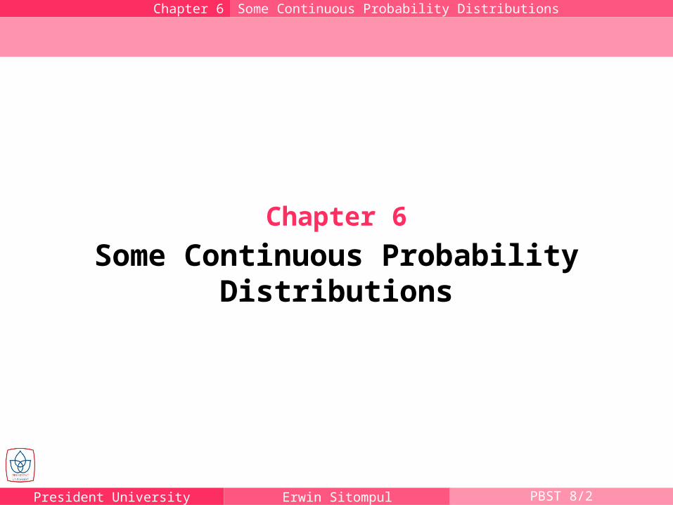
Continuous Uniform Distribution |Uniform Distribution| The density function of the continuous
uniform random variable X on the interval [A, B] is
Chapter 6.1 Continuous Uniform Distribution
1,
( ; , )
0, elsewhere
A x BB Af x A B
The uniform density function for a random variable on the interval [1, 3]
The mean and variance of the uniform distribution are2
2 ( )
2 12
A B B A and

President University Erwin Sitompul PBST 8/4
Continuous Uniform DistributionChapter 6.1 Continuous Uniform Distribution
Suppose that a large conference room for a certain company can be reserved for no more than 4 hours. However, the use of the conference room is such that both long and short conference occur quite often. In fact, it can be assumed that length X of a conference has a uniform distribution on the interval [0, 4].(a) What is the probability density function?(b) What is the probability that any given conference lasts at least 3
hours?
(a)
(b)
1, 0 4
4( )
0, elsewhere
xf x
4
3
13
4P X dx
1
4

President University Erwin Sitompul PBST 8/5
Normal Distribution Normal distribution is the most important continuous probability
distribution in the entire field of statistics. Its graph, called the normal curve, is the bell-shaped curve which
describes approximately many phenomena that occur in nature, industry, and research.
The normal distribution is often referred to as the Gaussian distribution, in honor of Karl Friedrich Gauss, who also derived its equation from a study of errors in repeated measurements of the same quantity.
Chapter 6.2 Normal Distribution
The normal curve

President University Erwin Sitompul PBST 8/6
Normal Distribution A continuous random variable X having the bell-shaped distribution
as shown on the figure is called a normal random variable.
21
21( ; , ) ,
2
x
n x e x
where π = 3.14159... and e = 2.71828...
Chapter 6.2 Normal Distribution
The density function of the normal random variable X, with mean μ and variance σ2, is

President University Erwin Sitompul PBST 8/7
Normal Curve
μ1 < μ2, σ1 = σ2 μ1 = μ2, σ1 < σ2
μ1 < μ2, σ1 < σ2
Chapter 6.2 Normal Distribution

President University Erwin Sitompul PBST 8/8
Normal CurveChapter 6.2 Normal Distribution
σ σ
x
f(x)
μ
The mode, the point where the curve is at maximum
Symmetry about a vertical axis through the mean μ
Point of inflection
Concave downward
Concave upward
Approaches zero asymptotically
Total area under the curve and above the horizontal axis is equal to 1
President University Erwin Sitompul PBST 8/9
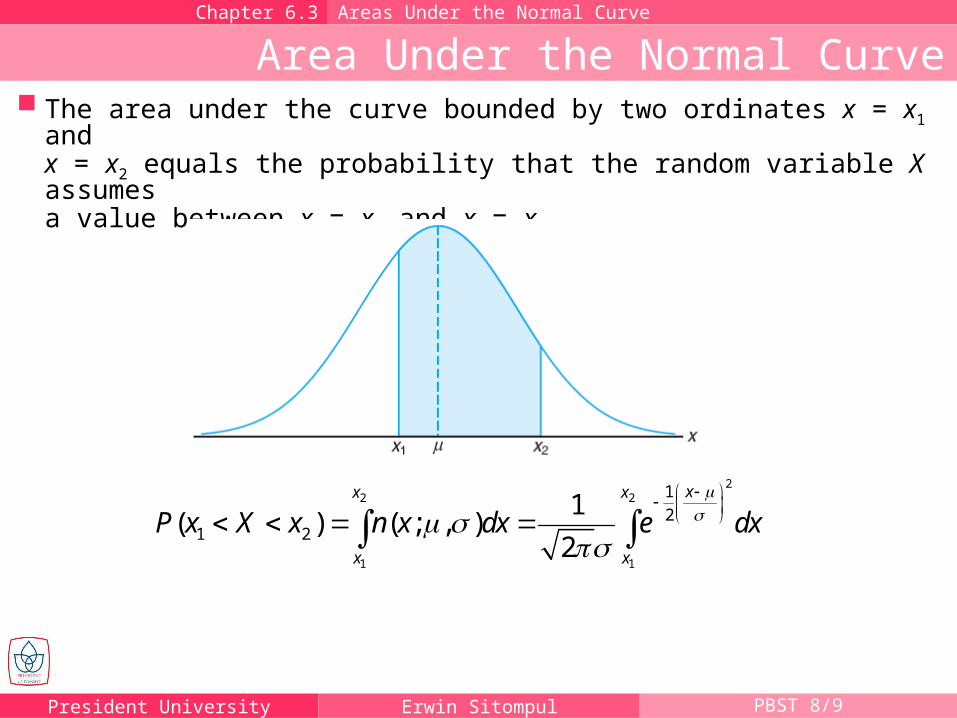
Area Under the Normal Curve The area under the curve bounded by two ordinates x = x1 and
x = x2 equals the probability that the random variable X assumes a value between x = x1 and x = x2.
Chapter 6.3 Areas Under the Normal Curve
22 2
1 1
1
21 2
1( ) ( ; , )
2
xx x
x x
P x X x n x dx e dx
President University Erwin Sitompul PBST 8/10
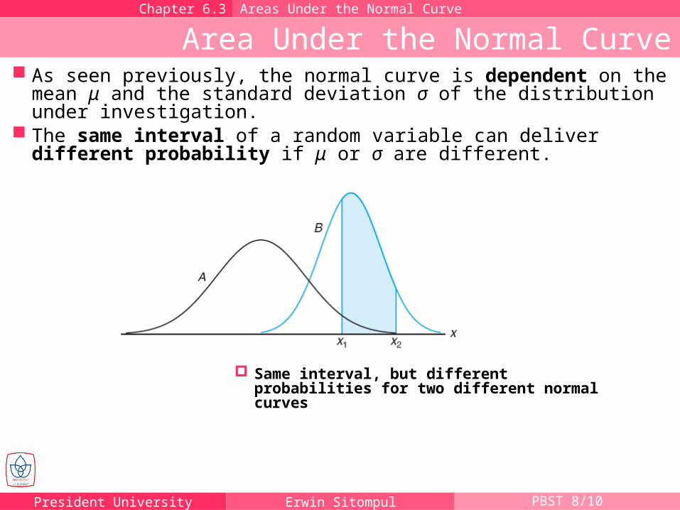
Area Under the Normal Curve As seen previously, the normal curve is dependent on the mean μ
and the standard deviation σ of the distribution under investigation.
The same interval of a random variable can deliver different probability if μ or σ are different.
Chapter 6.3 Areas Under the Normal Curve
Same interval, but different probabilities for two different normal curves
President University Erwin Sitompul PBST 8/11
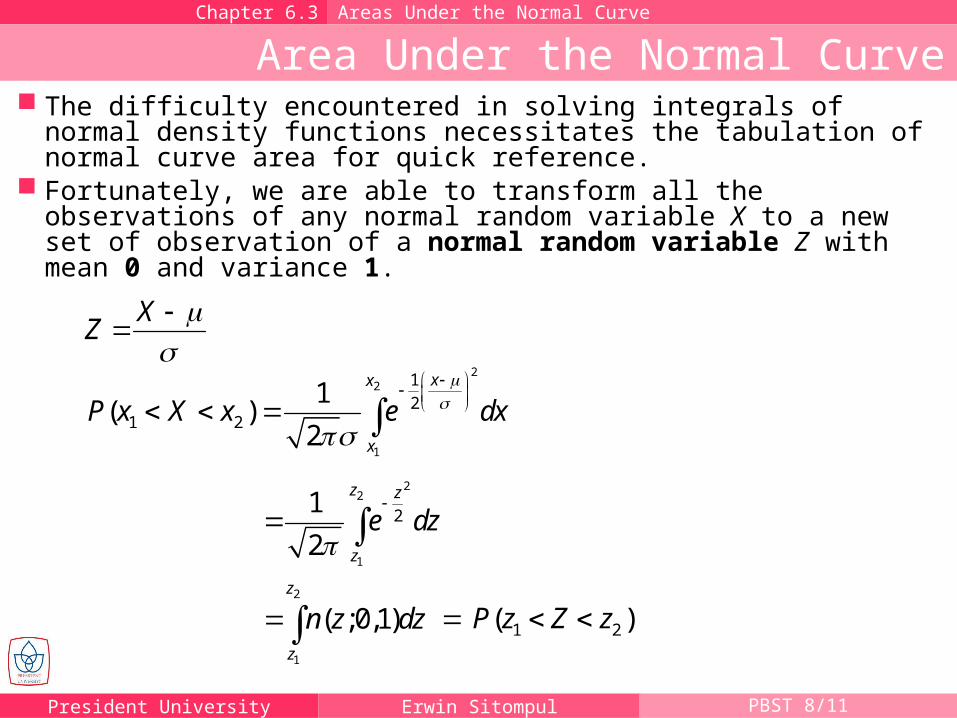
Area Under the Normal Curve The difficulty encountered in solving integrals of normal density
functions necessitates the tabulation of normal curve area for quick reference.
Fortunately, we are able to transform all the observations of any normal random variable X to a new set of observation of a normal random variable Z with mean 0 and variance 1.
Chapter 6.3 Areas Under the Normal Curve
XZ
2
2
1
1
21 2
1( )
2
xx
x
P x X x e dx
22
1
21
2
z z
z
e dz
2
1
( ;0,1)z
z
n z dz 1 2( )P z Z z
President University Erwin Sitompul PBST 8/12
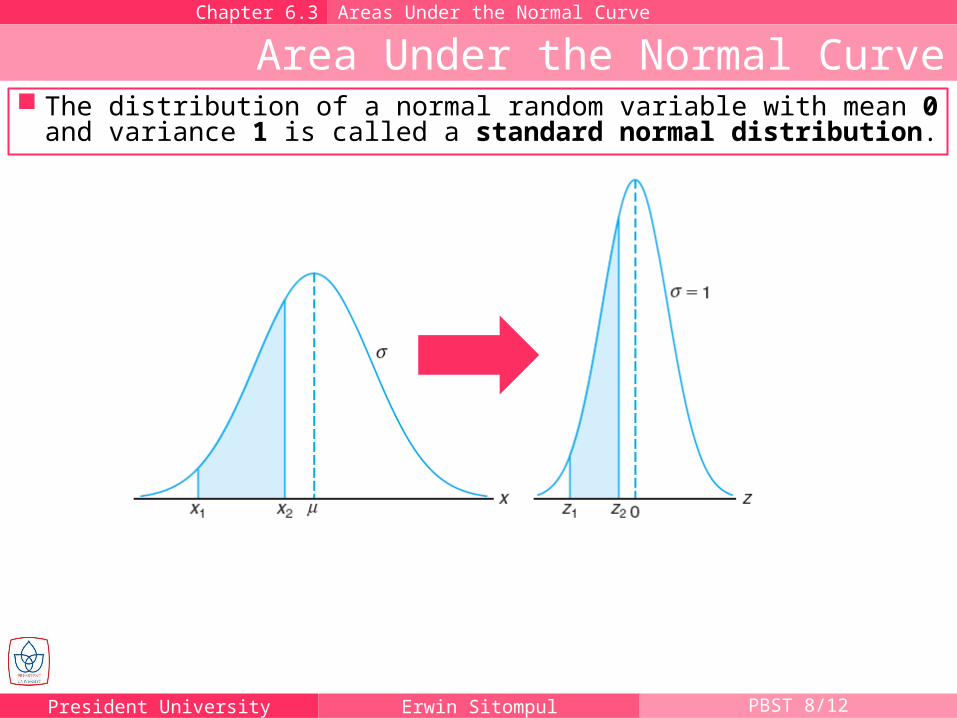
Area Under the Normal Curve The distribution of a normal random variable with mean 0 and
variance 1 is called a standard normal distribution.
Chapter 6.3 Areas Under the Normal Curve
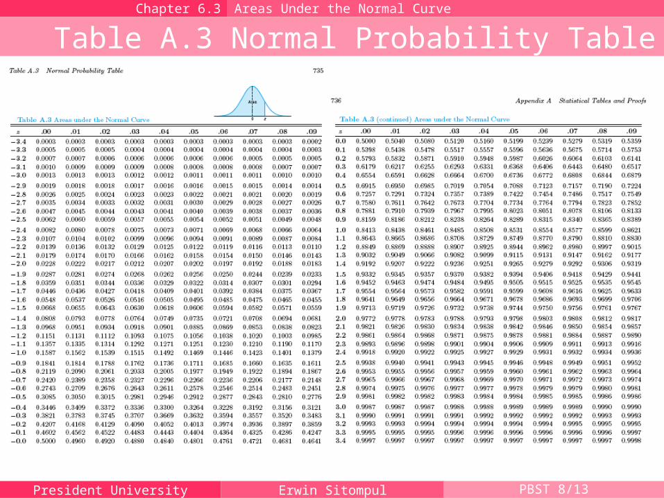
President University Erwin Sitompul PBST 8/13
Table A.3 Normal Probability TableChapter 6.3 Areas Under the Normal Curve
President University Erwin Sitompul PBST 8/14
InterpolationChapter 6.3 Areas Under the Normal Curve
a
( )f a
b
( )f b
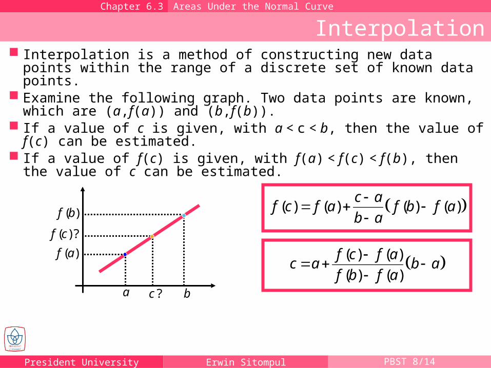
Interpolation is a method of constructing new data points within the range of a discrete set of known data points.
Examine the following graph. Two data points are known, which are (a,f(a)) and (b,f(b)).
If a value of c is given, with a < c < b, then the value of f(c) can be estimated.
If a value of f(c) is given, with f(a) < f(c) < f(b), then the value of c can be estimated.
?c
( )?f c
( ) ( ) ( ) ( )c a
f c f a f b f ab a
( ) ( )
( ) ( )
f c f ac a b a
f b f a
President University Erwin Sitompul PBST 8/15
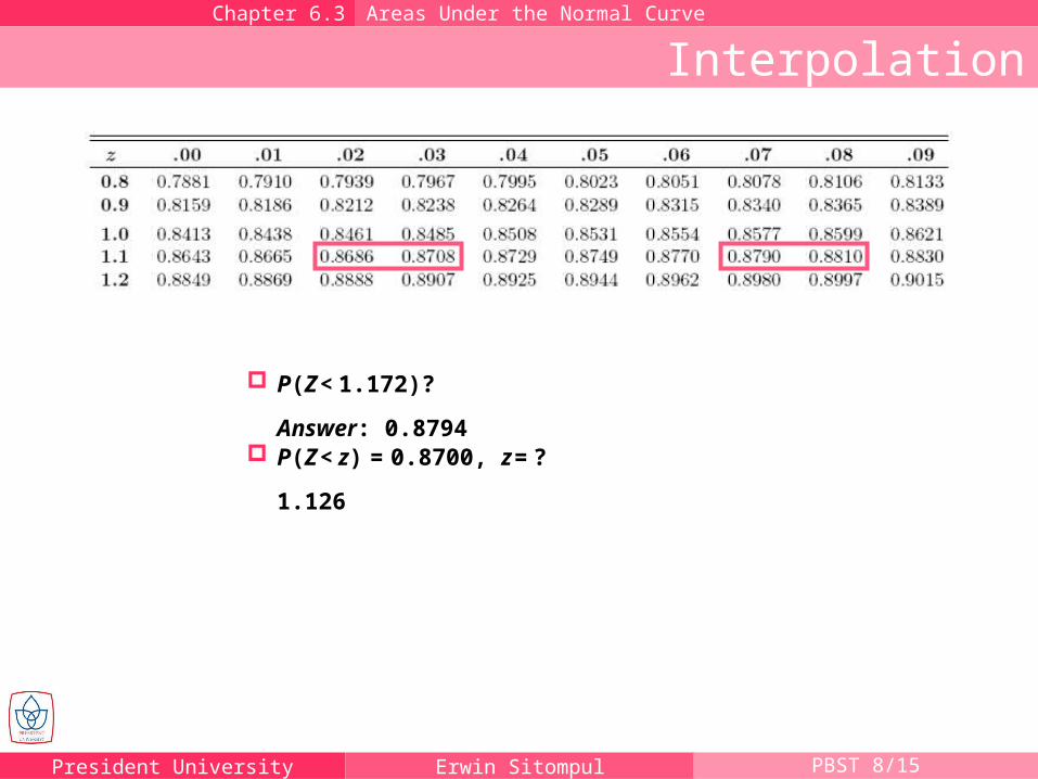
InterpolationChapter 6.3 Areas Under the Normal Curve
P(Z < 1.172)?
Answer: 0.8794 P(Z < z) = 0.8700, z = ?
1.126
President University Erwin Sitompul PBST 8/16
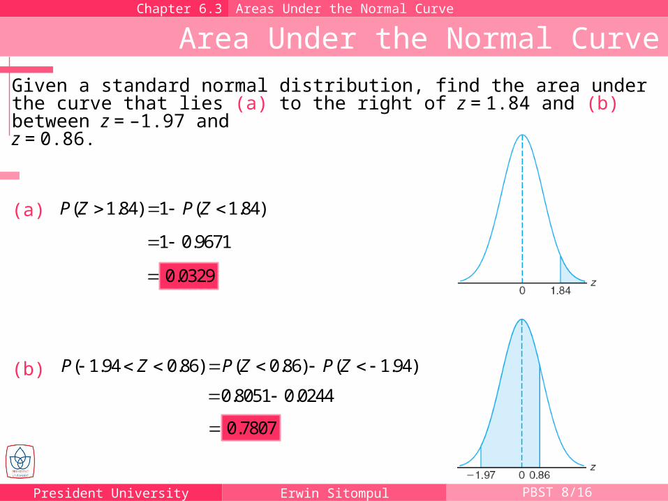
Area Under the Normal CurveChapter 6.3 Areas Under the Normal Curve
Given a standard normal distribution, find the area under the curve that lies (a) to the right of z = 1.84 and (b) between z = –1.97 and z = 0.86.
(a)
(b)
( 1.84) 1 ( 1.84)P Z P Z
1 0.9671
0.0329
( 1.94 0.86) ( 0.86) ( 1.94)P Z P Z P Z
0.8051 0.0244
0.7807

President University Erwin Sitompul PBST 8/17
Area Under the Normal CurveChapter 6.3 Areas Under the Normal Curve
Given a standard normal distribution, find the value of k such that (a) P ( Z > k ) = 0.3015, and (b) P ( k < Z < –0.18 ) = 0.4197.
(a)
(b)
( ) 1 ( )P Z k P Z k
( ) 1 ( )P Z k P Z k
0.52k
( 0.18) ( 0.18) ( )P k Z P Z P Z k
1 0.3015 0.6985
( ) ( 0.18) ( 0.18)P Z k P Z P k Z
0.4286 0.4197 0.0089
2.37k
President University Erwin Sitompul PBST 8/18
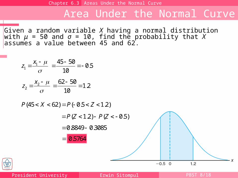
Area Under the Normal CurveChapter 6.3 Areas Under the Normal Curve
Given a random variable X having a normal distribution with μ = 50 and σ = 10, find the probability that X assumes a value between 45 and 62.
11
xz
(45 62) ( 0.5 1.2)P X P Z
22
xz
( 1.2) ( 0.5)P Z P Z
0.8849 0.3085
0.5764
45 500.5
10
62 501.2
10
President University Erwin Sitompul PBST 8/19
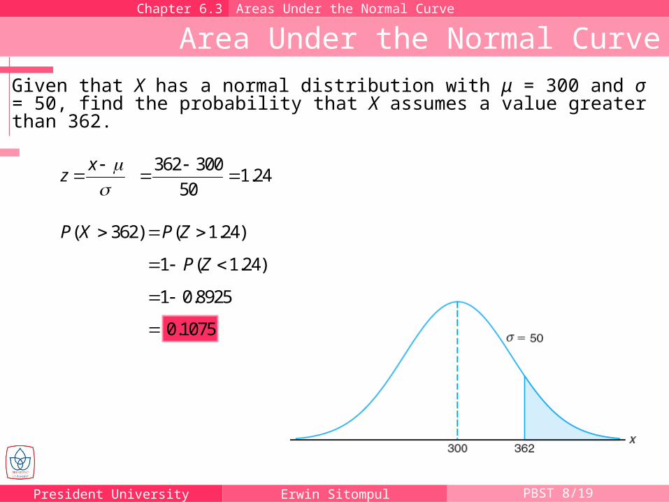
Area Under the Normal CurveChapter 6.3 Areas Under the Normal Curve
Given that X has a normal distribution with μ = 300 and σ = 50, find the probability that X assumes a value greater than 362.
xz
( 362) ( 1.24)P X P Z
1 0.8925
1 ( 1.24)P Z
0.1075
362 3001.24
50
President University Erwin Sitompul PBST 8/20
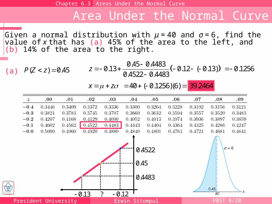
Area Under the Normal CurveChapter 6.3 Areas Under the Normal Curve
Given a normal distribution with μ = 40 and σ = 6, find the value of x that has (a) 45% of the area to the left, and (b) 14% of the area to the right.
(a) ( ) 0.45P Z z 0.45 0.44830.13 0.12 ( 0.13)
0.4522 0.4483z
0.1256
x z
0.13
0.4483
0.12
0.4522
?
0.45
40 ( 0.1256)(6) 39.2464
President University Erwin Sitompul PBST 8/21
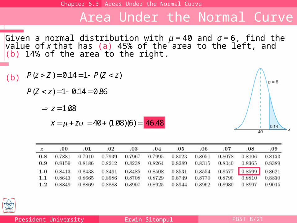
Area Under the Normal CurveChapter 6.3 Areas Under the Normal Curve
Given a normal distribution with μ = 40 and σ = 6, find the value of x that has (a) 45% of the area to the left, and (b) 14% of the area to the right.
(b) ( ) 0.14 1 ( )P z Z P Z z
( ) 1 0.14 0.86P Z z
1.08z
x z 40 (1.08)(6) 46.48
President University Erwin Sitompul PBST 8/22
Applications of the Normal DistributionChapter 6.4 Applications of the Normal Distribution
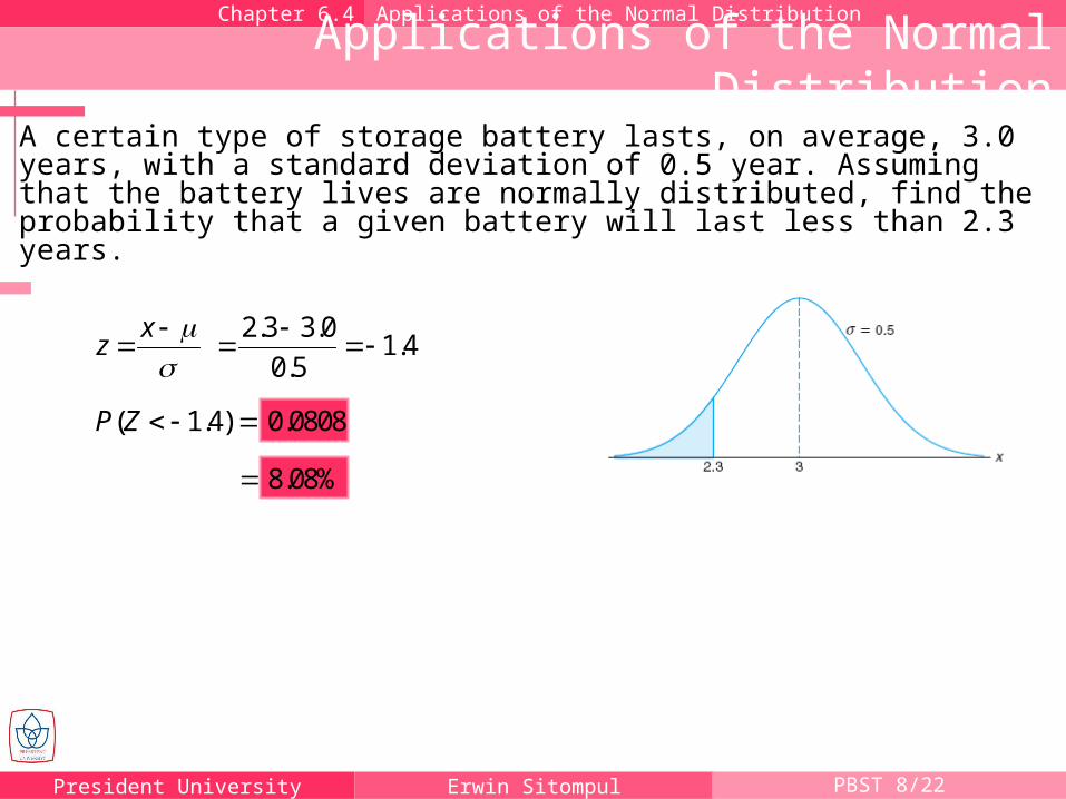
A certain type of storage battery lasts, on average, 3.0 years, with a standard deviation of 0.5 year. Assuming that the battery lives are normally distributed, find the probability that a given battery will last less than 2.3 years.
( 1.4) 0.0808P Z
xz
2.3 3.0
1.40.5
8.08%
President University Erwin Sitompul PBST 8/23
Applications of the Normal DistributionChapter 6.4 Applications of the Normal Distribution
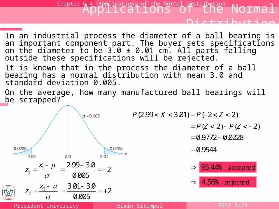
In an industrial process the diameter of a ball bearing is an important component part. The buyer sets specifications on the diameter to be 3.0 ± 0.01 cm. All parts falling outside these specifications will be rejected. It is known that in the process the diameter of a ball bearing has a normal distribution with mean 3.0 and standard deviation 0.005. On the average, how many manufactured ball bearings will be scrapped?
11
xz
22
xz
(2.99 3.01) ( 2 2)P X P Z
( 2) ( 2)P Z P Z 0.9772 0.0228
0.9544
4.56% rejected
2.99 3.02
0.005
3.01 3.02
0.005
95.44% accepted
President University Erwin Sitompul PBST 8/24
Applications of the Normal DistributionChapter 6.4 Applications of the Normal Distribution
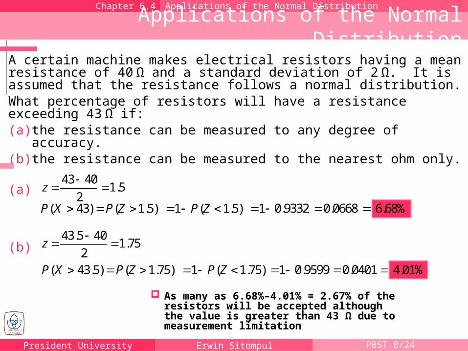
A certain machine makes electrical resistors having a mean resistance of 40 Ω and a standard deviation of 2 Ω. It is assumed that the resistance follows a normal distribution.What percentage of resistors will have a resistance exceeding 43 Ω if:(a) the resistance can be measured to any degree of accuracy.(b) the resistance can be measured to the nearest ohm only.
43 401.5
2z
( 43) ( 1.5)P X P Z 1 ( 1.5)P Z 1 0.9332 0.0668 6.68%(a)
(b)
( 43.5) ( 1.75)P X P Z 1 ( 1.75)P Z 1 0.9599 0.0401 4.01%
43.5 401.75
2z
As many as 6.68%–4.01% = 2.67% of the resistors will be accepted although the value is greater than 43 Ω due to measurement limitation
President University Erwin Sitompul PBST 8/25
Applications of the Normal DistributionChapter 6.4 Applications of the Normal Distribution
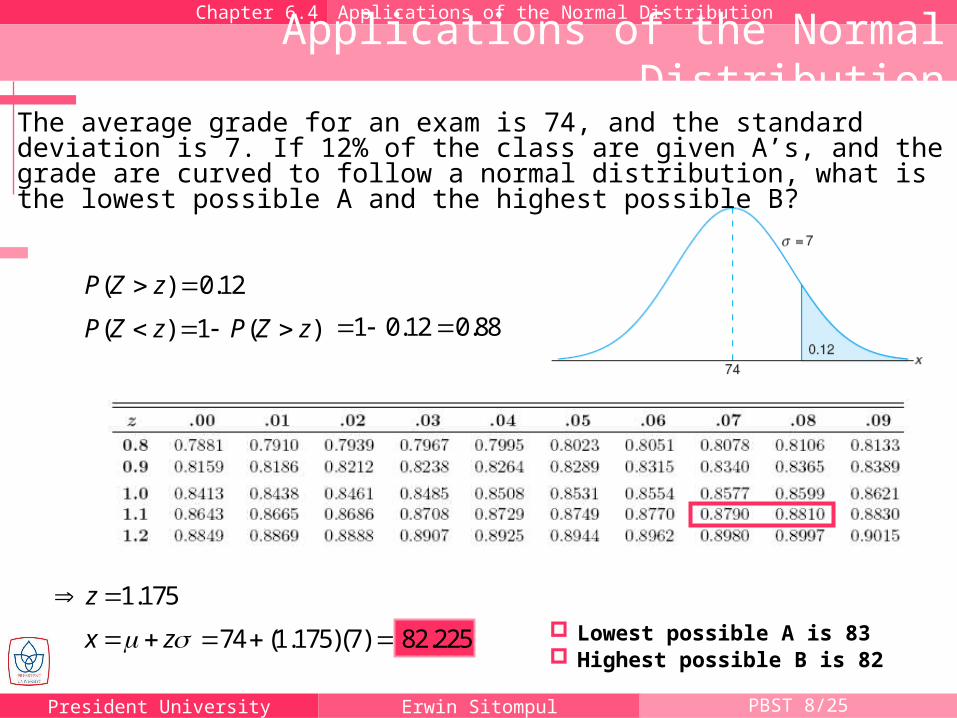
The average grade for an exam is 74, and the standard deviation is 7. If 12% of the class are given A’s, and the grade are curved to follow a normal distribution, what is the lowest possible A and the highest possible B?
( ) 0.12P Z z
( ) 1 ( )P Z z P Z z 1 0.12 0.88
1.175z
x z Lowest possible A is 83 Highest possible B is 82
74 (1.175)(7) 82.225
President University Erwin Sitompul PBST 8/26
Homework 7AProbability and Statistics
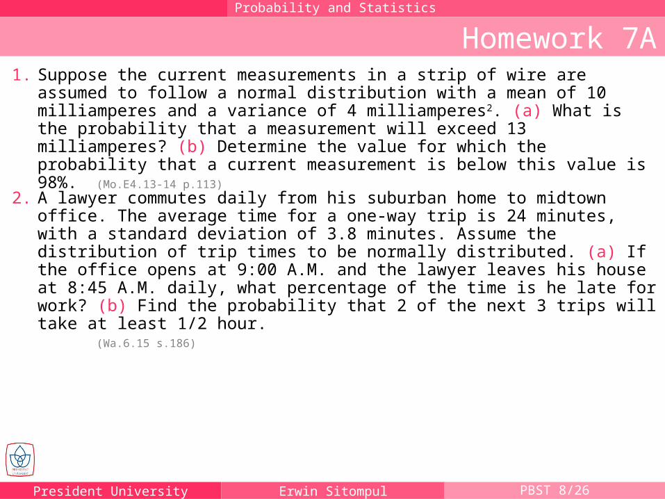
1. Suppose the current measurements in a strip of wire are assumed to follow a normal distribution with a mean of 10 milliamperes and a variance of 4 milliamperes2. (a) What is the probability that a measurement will exceed 13 milliamperes? (b) Determine the value for which the probability that a current measurement is below this value is 98%. (Mo.E4.13-14 p.113)
2. A lawyer commutes daily from his suburban home to midtown office. The average time for a one-way trip is 24 minutes, with a standard deviation of 3.8 minutes. Assume the distribution of trip times to be normally distributed. (a) If the office opens at 9:00 A.M. and the lawyer leaves his house at 8:45 A.M. daily, what percentage of the time is he late for work? (b) Find the probability that 2 of the next 3 trips will take at least 1/2 hour.
(Wa.6.15 s.186)