Embed Size (px)
Citation preview
President University Erwin Sitompul Modern Control 11/1
Dr.-Ing. Erwin SitompulPresident University
Lecture 11Modern Control
http://zitompul.wordpress.com
President University Erwin Sitompul Modern Control 11/2
Homework 9Chapter 10 Optimal Control
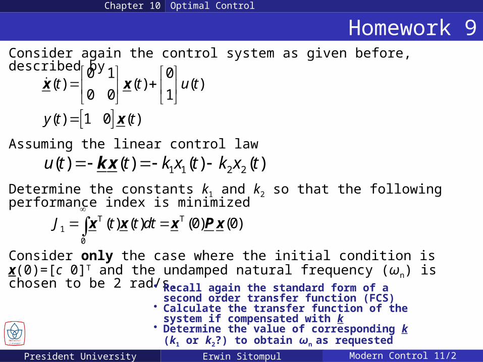
Consider again the control system as given before, described by
0 1 0( ) ( ) ( )
0 0 1
( ) 1 0 ( )
t t u t
y t t
x x
x
Assuming the linear control law
1 1 2 2( ) ( ) ( ) ( )u t t k x t k x t k x
Determine the constants k1 and k2 so that the following performance index is minimized
T T1
0
( ) ( ) (0) (0)J t t dt
x x x P x
Consider only the case where the initial condition is x(0)=[c 0]T and the undamped natural frequency (ωn) is chosen to be 2 rad/s.
• Recall again the standard form of a second order transfer function (FCS)
• Calculate the transfer function of the system if compensated with k
• Determine the value of corresponding k (k1 or k2?) to obtain ωn as requested
President University Erwin Sitompul Modern Control 11/3
Solution of Homework 9Chapter 10 Optimal Control
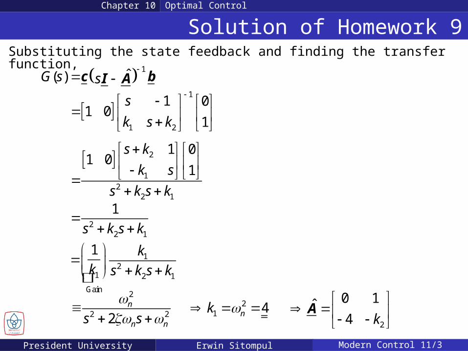
Substituting the state feedback and finding the transfer function,
1ˆ( )G s s
c bI A
1
1 2
1 01 0
1
s
k s k
2
12
2 1
1 01 0
1
s k
k s
s k s k
22 1
1
s k s k
2
2 22n
n ns s
12
1 2 1
Gain
1 kk s k s k
21 4nk
2
0 1ˆ4 k
A
President University Erwin Sitompul Modern Control 11/4
Solution of Homework 9Chapter 10 Optimal Control
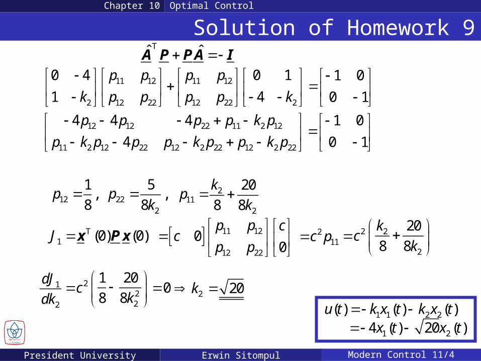
Tˆ ˆ A P PA I
11 12 11 12
2 12 22 12 22 2
0 4 0 1 1 0
1 4 0 1
p p p p
k p p p p k
12 12 22 11 2 12
11 2 12 22 12 2 22 12 2 22
4 4 4 1 0
4 0 1
p p p p k p
p k p p p k p p k p
12
1,
8p 2
112
20
8 8
kp
k 22
2
5,
8p
k
T1 (0) (0)J x P x 11 12
12 22
00
p p cc
p p
2
11c p 2 2
2
20
8 8
kc
k
21222
1 200
8 8dJ
ckdk
2 20k
1 1 2 2( ) ( ) ( )u t k x t k x t
1 24 ( ) 20 ( )x t x t
President University Erwin Sitompul Modern Control 11/5
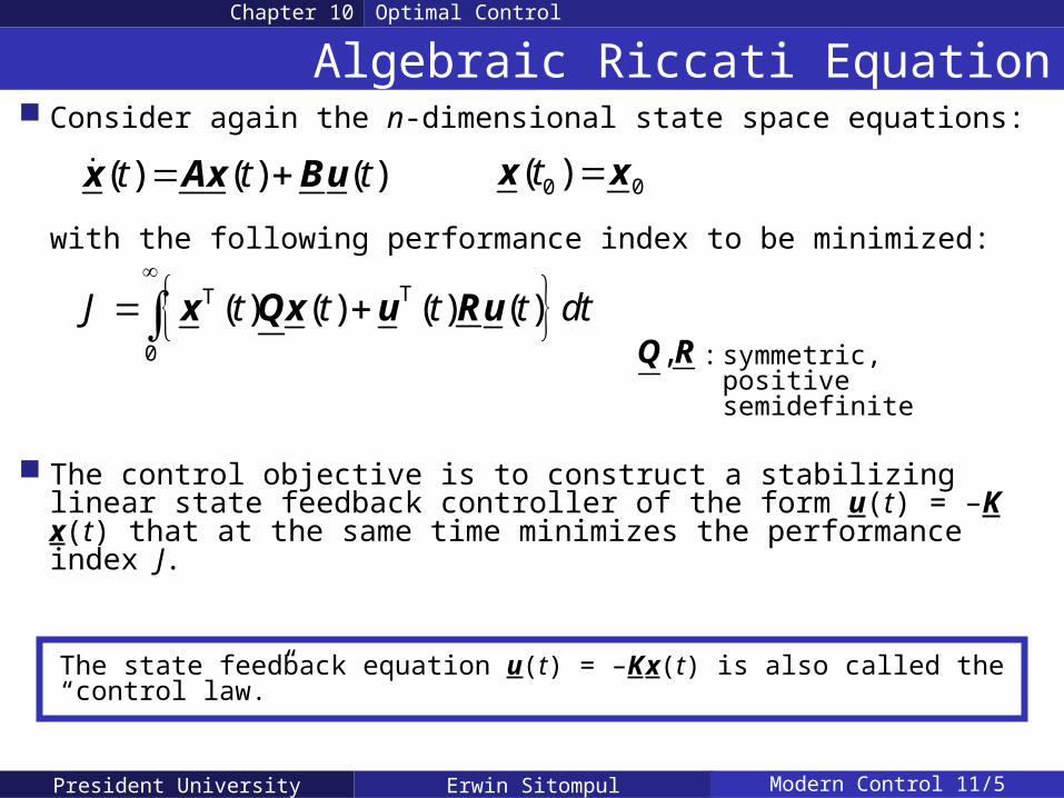
Algebraic Riccati Equation Consider again the n-dimensional state space equations:
Chapter 10 Optimal Control
( ) ( ) ( )t t t x Ax Bu 00( )t x x
with the following performance index to be minimized:
TT
0
( ) ( ) ( ) ( )J t t t t dt
x Qx u Ru,Q R : symmetric, positive
semidefinite
The control objective is to construct a stabilizing linear state feedback controller of the form u(t) = –K x(t) that at the same time minimizes the performance index J.
The state feedback equation u(t) = –K x(t) is also called the “control law.”
President University Erwin Sitompul Modern Control 11/6
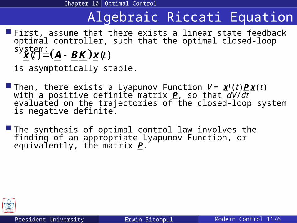
First, assume that there exists a linear state feedback optimal controller, such that the optimal closed-loop system:
Chapter 10 Optimal Control
( ) ( )t t x A BK xis asymptotically stable.
Then, there exists a Lyapunov Function V = xT(t)P x(t) with a positive definite matrix P, so that dV/dt evaluated on the trajectories of the closed-loop system is negative definite.
Algebraic Riccati Equation
The synthesis of optimal control law involves the finding of an appropriate Lyapunov Function, or equivalently, the matrix P.
President University Erwin Sitompul Modern Control 11/7
Chapter 10 Optimal Control
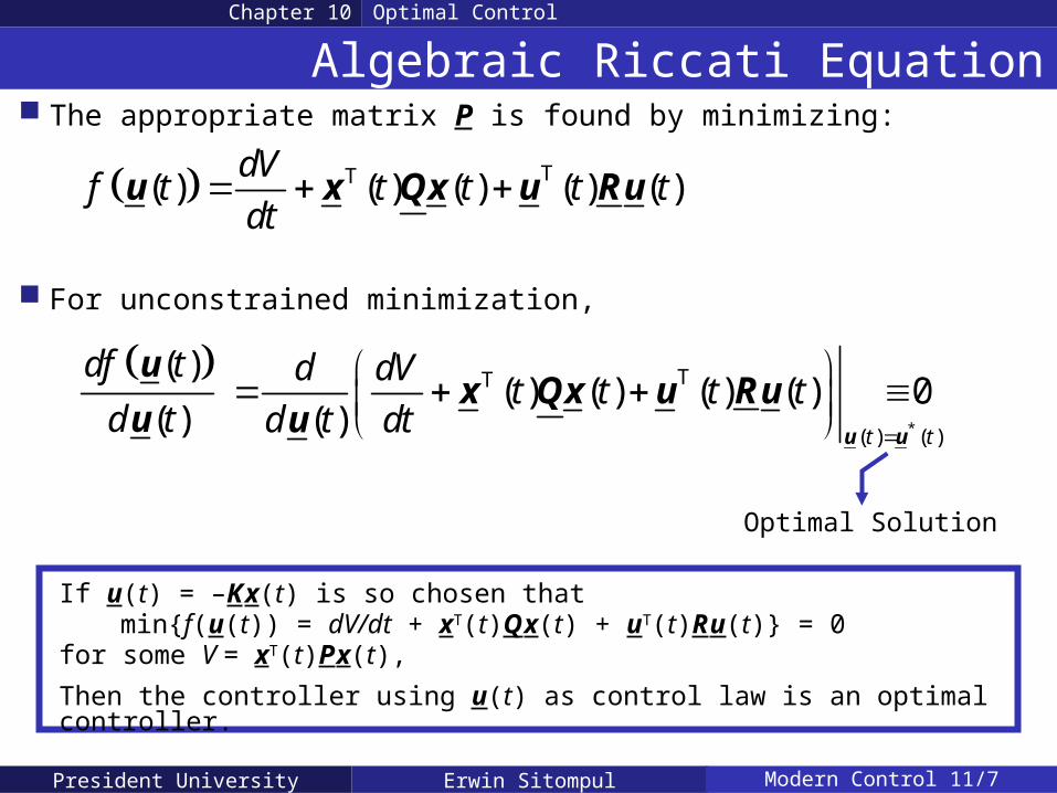
The appropriate matrix P is found by minimizing:
Algebraic Riccati Equation
TT( ) ( ) ( ) ( ) ( )dV
f t t t t tdt
u x Qx u Ru
If u(t) = –K x(t) is so chosen thatmin{f(u(t)) = dV/dt + xT(t)Q x(t) + uT(t)R u(t)} = 0
for some V = xT(t)P x(t),
Then the controller using u(t) as control law is an optimal controller.
For unconstrained minimization,
( )
( )
df t
d t
u
u *
TT
( ) ( )
( ) ( ) ( ) ( )( ) t t
d dVt t t t
d t dt
u u
x Qx u Ruu
0
Optimal Solution
President University Erwin Sitompul Modern Control 11/8
Chapter 10 Optimal Control
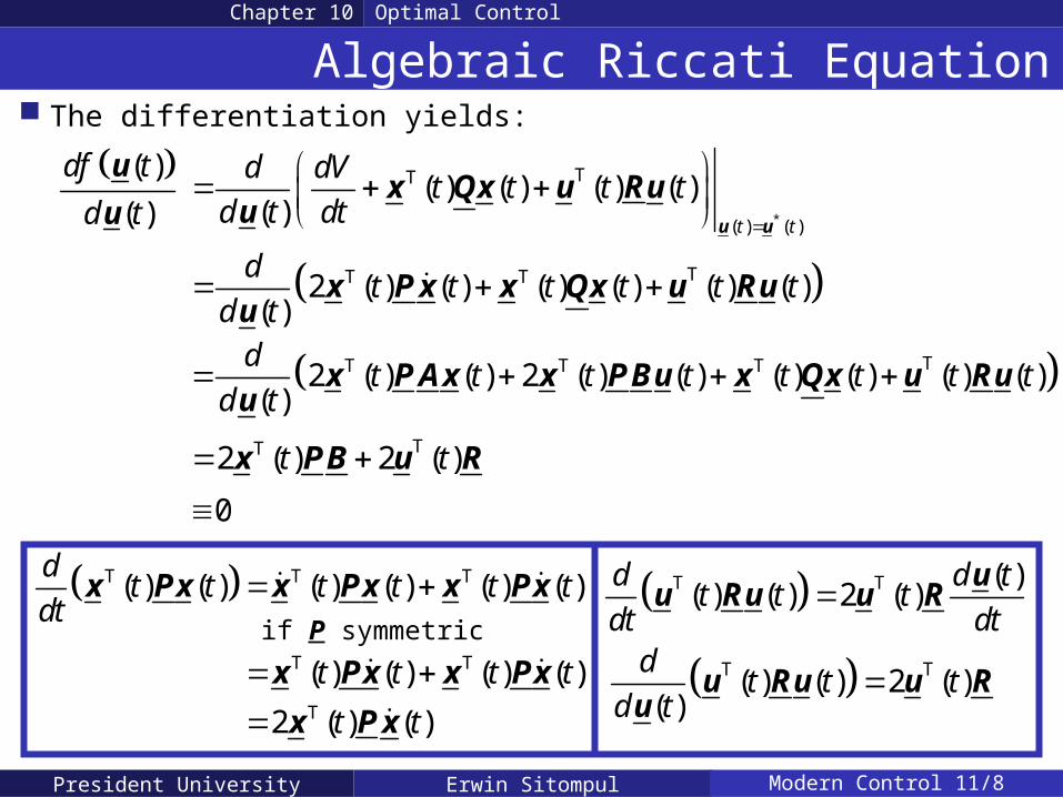
Algebraic Riccati Equation The differentiation yields:
( )
( )
df t
d t
u
u *
TT
( ) ( )
( ) ( ) ( ) ( )( ) t t
d dVt t t t
d t dt
u u
x Qx u Ruu
TT T2 ( ) ( ) ( ) ( ) ( ) ( )( )
dt t t t t t
d t x P x x Qx u Ruu
TT T T2 ( ) ( ) 2 ( ) ( ) ( ) ( ) ( ) ( )( )
dt t t t t t t t
d t x PAx x PBu x Qx u Ruu
TT2 ( ) 2 ( )t t x PB u R
0
T T T( ) ( ) ( ) ( ) ( ) ( )d
t t t t t tdt
x Px x Px x Px
T T( ) ( ) ( ) ( )t t t t x Px x PxT2 ( ) ( )t t x P x
if P symmetric T T ( )
( ) ( ) 2 ( )d d t
t t tdt dt
u
u Ru u R
T T( ) ( ) 2 ( )( )
dt t t
d tu Ru u R
u
President University Erwin Sitompul Modern Control 11/9
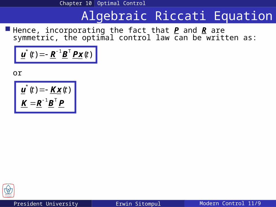
Hence, incorporating the fact that P and R are symmetric, the optimal control law can be written as:
* 1 T( ) ( )t tu R B Px
or
*( ) ( )t tu Kx1 TK R B P
Algebraic Riccati EquationChapter 10 Optimal Control
President University Erwin Sitompul Modern Control 11/10
Algebraic Riccati EquationChapter 10 Optimal Control
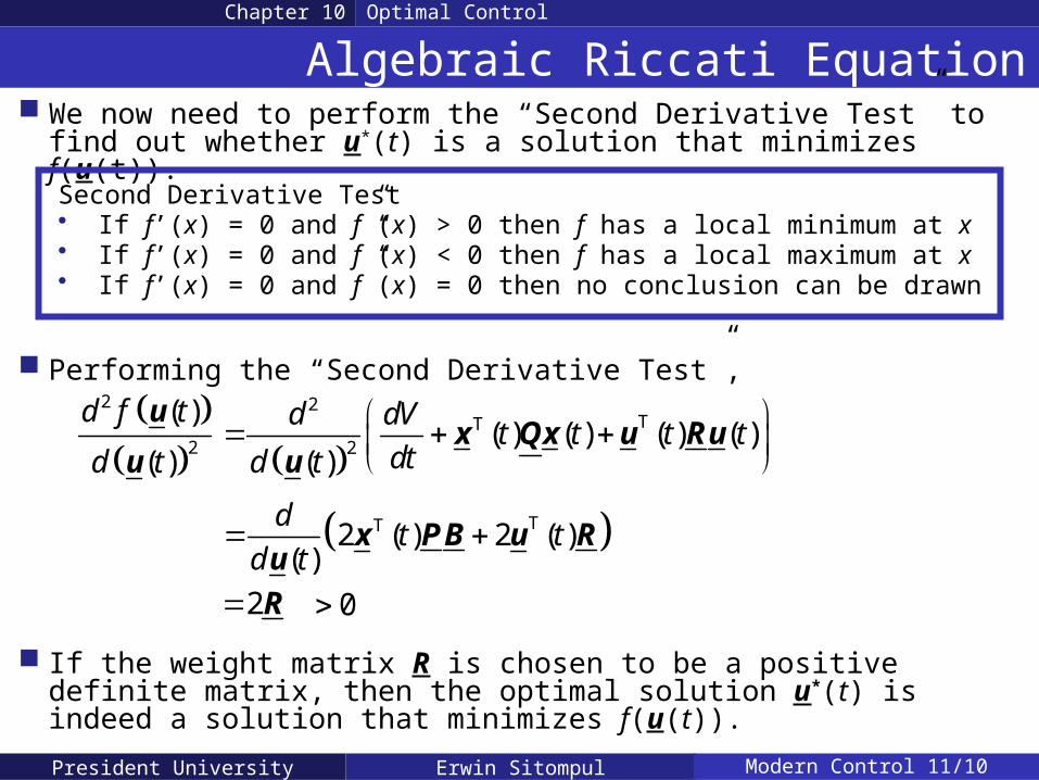
Performing the “Second Derivative Test”,
2
2
( )
( )
d f t
d t
u
u
2TT
2 ( ) ( ) ( ) ( )( )
d dVt t t t
dtd t
x Qx u Ruu
TT2 ( ) 2 ( )( )
dt t
d t x PB u Ru
2 R 0
If the weight matrix R is chosen to be a positive definite matrix, then the optimal solution u*(t) is indeed a solution that minimizes f(u(t)).
We now need to perform the “Second Derivative Test” to find out whether u*(t) is a solution that minimizes f(u(t)).
Second Derivative Test• If f’(x) = 0 and f”(x) > 0 then f has a local minimum at x• If f’(x) = 0 and f”(x) < 0 then f has a local maximum at x• If f’(x) = 0 and f”(x) = 0 then no conclusion can be drawn
President University Erwin Sitompul Modern Control 11/11
Algebraic Riccati EquationChapter 10 Optimal Control
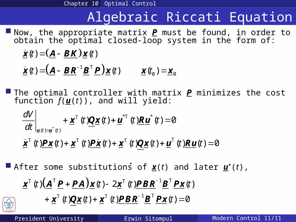
Now, the appropriate matrix P must be found, in order to obtain the optimal closed-loop system in the form of:
( ) ( )t t x A BK x
1 T( ) ( )t t x A BR B P x 00( )t x x
The optimal controller with matrix P minimizes the cost function f(u(t)), and will yield:
*
*T *T
( ) ( )
( ) ( ) ( ) ( ) 0t t
dVt t t t
dt
u u
x Qx u Ru
TT T T( ) ( ) ( ) ( ) ( ) ( ) ( ) ( ) 0t t t t t t t t x Px x Px x Qx u Ru
After some substitutions of x(t) and later u*(t),
T 1 TT T
1 TT T
( ) ( ) 2 ( ) ( )
( ) ( ) ( ) ( ) 0
t t t t
t t t t
x A P PA x x PBR B Px
x Qx x PBR B Px
President University Erwin Sitompul Modern Control 11/12
Algebraic Riccati EquationChapter 10 Optimal Control
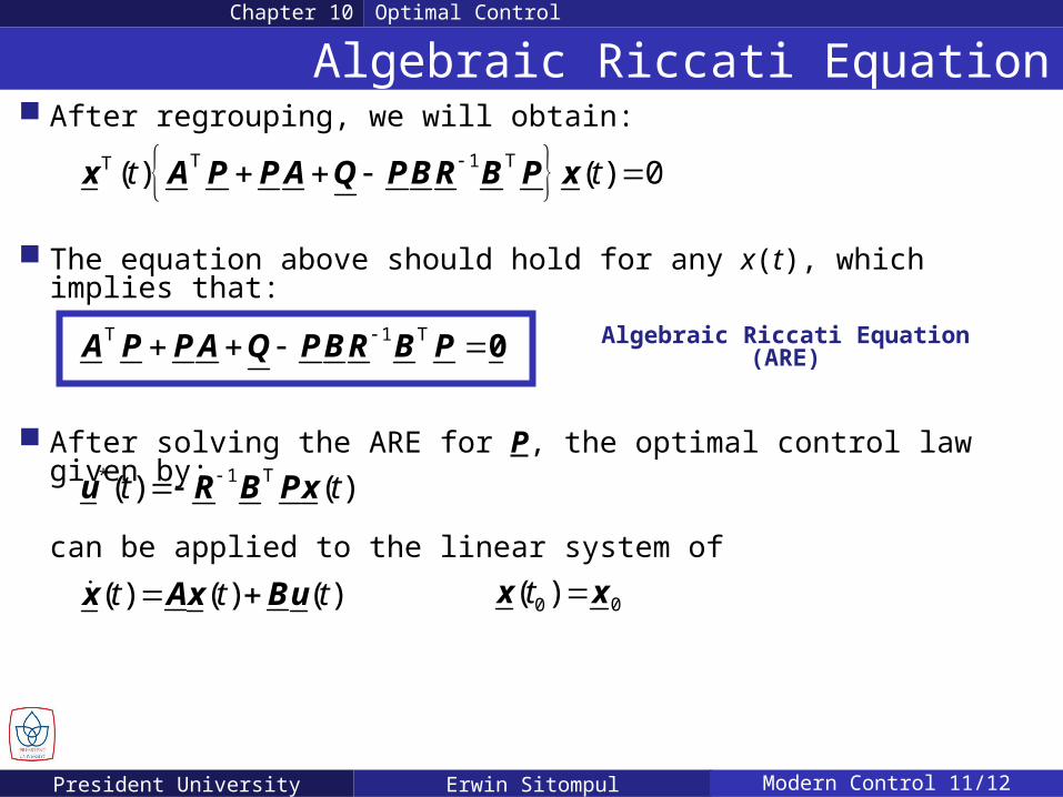
After regrouping, we will obtain:
T 1 TT ( ) ( ) 0t t x A P PA Q PBR B P x
The equation above should hold for any x(t), which implies that:
T 1 T A P PA Q PBR B P 0 Algebraic Riccati Equation (ARE)
After solving the ARE for P, the optimal control law given by:* 1 T( ) ( )t tu R B Px
can be applied to the linear system of
( ) ( ) ( )t t t x Ax Bu 00( )t x x
President University Erwin Sitompul Modern Control 11/13
1 TT 0A P PA Q P P BR B
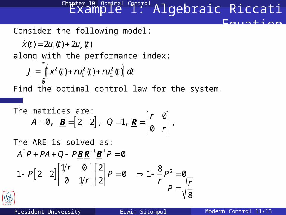
Example 1: Algebraic Riccati EquationChapter 10 Optimal Control
Consider the following model:
1 2( ) 2 ( ) 2 ( )x t u t u t along with the performance index:
2 2 21 2
0
( ) ( ) ( )J x t ru t ru t dt
Find the optimal control law for the system.
The matrices are:0,A 2 2 ,B 1,Q
0,
0
r
r
R
The ARE is solved as:
1 0 21 2 2 0
0 1 2
rP P
r
28
1 0Pr
8
rP
President University Erwin Sitompul Modern Control 11/14
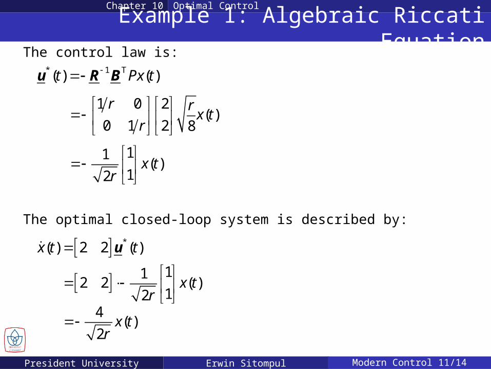
Example 1: Algebraic Riccati EquationChapter 10 Optimal Control
The control law is:* 1 T( ) ( )t Px tu R B
1 0 2( )
0 1 2 8
r rx t
r
11( )
12x t
r
The optimal closed-loop system is described by:
*( ) 2 2 ( )x t t u
112 2 ( )
12x t
r
4
( )2x t
r
President University Erwin Sitompul Modern Control 11/15
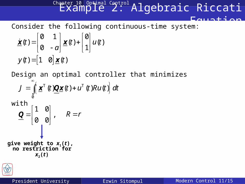
Example 2: Algebraic Riccati EquationChapter 10 Optimal Control
Consider the following continuous-time system:
Design an optimal controller that minimizes
with
0 1 0( ) ( ) ( )
0 1
( ) ( )1 0
t t u ta
y t t
x x
x
T T
0
( ) ( ) ( ) ( )J t t u t Ru t dt
x Qx
R r1 0
,0 0
Q
give weight to x1(t), no restriction for x2(t)
President University Erwin Sitompul Modern Control 11/16
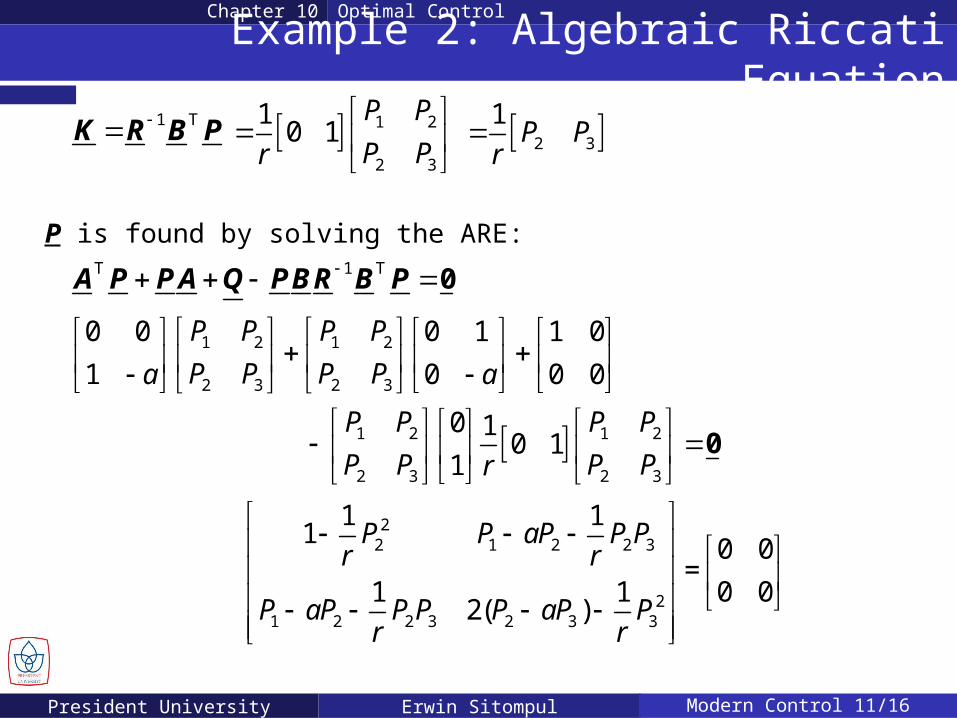
Example 2: Algebraic Riccati EquationChapter 10 Optimal Control
1 TK R B P 1 2
2 3
10 1
P P
P Pr
2 3
1P P
r
P is found by solving the ARE:T 1 T A P PA Q PBR B P 0
1 2 1 2
2 3 2 3
1 2 1 2
2 3 2 3
0 0 0 1 1 0
1 0 0 0
0 1 0 1
1
P P P P
P P P Pa a
P P P P
P P P Pr
0
22 1 2 2 3
21 2 2 3 2 3 3
1 11 0 0
=1 1 0 0
2( )
P P aP P Pr r
P aP P P P aP Pr r
President University Erwin Sitompul Modern Control 11/17
Example 2: Algebraic Riccati EquationChapter 10 Optimal Control
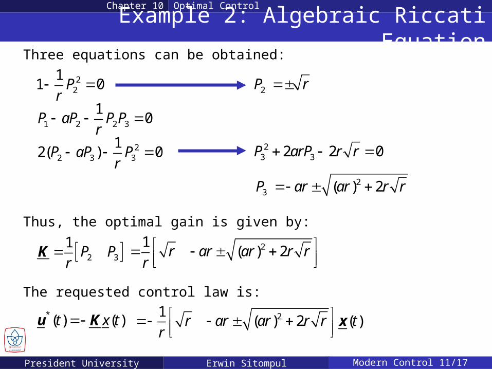
Three equations can be obtained:
22
11 0Pr
1 2 2 3
10P aP P P
r
22 3 3
12( ) 0P aP P
r
2P r
23 32 2 0P arP r r
23 ( ) 2P ar ar r r
2 3
1P P
rK 21
( ) 2r ar ar r rr
Thus, the optimal gain is given by:
The requested control law is:
*( ) ( )t x tu K 21( ) 2 ( )r ar ar r r t
r
x
President University Erwin Sitompul Modern Control 11/18
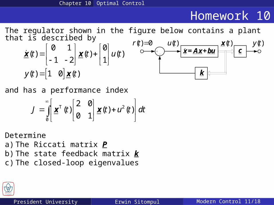
Homework 10Chapter 10 Optimal Control
The regulator shown in the figure below contains a plant that is described by
0 1 0( ) ( ) ( )
1 2 1
( ) 1 0 ( )
t t u t
y t t
x x
x
T 2
0
2 0( ) ( ) ( )
0 1J t t u t dt
x x
and has a performance index
Determinea) The Riccati matrix Pb) The state feedback matrix kc) The closed-loop eigenvalues
( )u t+–
( ) 0r t x= Ax+bu
k
c( )y t( )tx