PREPRINT 2012:11

Modelling of road profiles using roughness indicators

PÄR JOHANNESSON IGOR RYCHLIK Department of Mathematical Sciences Division of Mathematics

CHALMERS UNIVERSITY OF TECHNOLOGY UNIVERSITY OF GOTHENBURG Gothenburg Sweden 2012

Preprint 2012:11

Modelling of road profiles using roughness indicators

Pär Johannesson and Igor Rychlik

Department of Mathematical Sciences Division of Mathematics

Chalmers University of Technology and University of Gothenburg SE-412 96 Gothenburg, Sweden Gothenburg, August 2012

Preprint 2012:11

ISSN 1652-9715

Matematiska vetenskaper

Göteborg 2012

Modelling of road profiles using roughness indicators

PÄR JOHANNESSON∗ AND IGOR RYCHLIK ∗∗

Addresses:∗ SP Technical Research Institute of Sweden, SE-400 22 Göteborg, Sweden (Corresponding author)

Par.Johannesson@sp.se∗∗ Mathematical Sciences, Chalmers University of Technology, SE-412 96 Göteborg, Sweden

rychlik@chalmers.se

Abstract

The vertical road input is the most important load for durability assessments of vehicles. Wefocus on stochastic modelling of the road profile with the aimto find a simple by still usefulmodel. The proposed non-stationary Laplace model with ISO spectrum has only two param-eters, and can be efficiently estimated from a sequence of roughness indicators, such as IRIor ISO roughness coefficient. Thus, a road profile can be stochastically reconstructed fromroughness indicators. Further, explicit approximations for the fatigue damage due to Laplaceroads are developed. The usefulness of the proposed Laplace-ISO model is validated for eightmeasured road profiles.

Keywords: Road surface profile, road roughness, road irregularity, Laplace process, non-Gaussian process, power spectral density (PSD), ISO spectrum, roughness coefficient, inter-national roughness index (IRI), vehicle durability, fatigue damage.

1 Introduction

Durability assessment of vehicle components often requires a customer or market specific loaddescription. It is therefore desirable to have a model of theload environment that is vehicleindependent and which may include many factors, such as encountered road roughness, hilli-ness, curvature, cargo loading, driver behaviour and legislation. Here we are concerned withmodelling of the road surface roughness with focus on fatigue life prediction. Especially, wefocus on reconstruction of road profiles based on measurements of the so-called InternationalRoughness Index (IRI), which is often available from road administration data bases.

Traditionally, road profiles have been modelled by using Gaussian processes, see e.g.(Dodds and Robson, 1973; ISO 8608, 1995; Andrén, 2006). However, it is well known thatmeasured road profiles contain shorter segments with above average irregularity, which is aproperty that can not be modelled by a Gaussian process, and therefore several approaches hasbeen suggested, see e.g. (Bogsjö, 2007) and the references therein. In (Bogsjö et al., 2012) anew class of random processes, namely Laplace processes, has been proposed for modellingroad profiles. Simply speaking it is a Gaussian process wherethe variance is randomly chang-ing. A similar approach has been taken by (Bruscella et al., 1999; Rouillard, 2004, 2009).

In the case when only IRI data available, a simple enough model is required in order tobe able to estimate the model parameters. Therefore, we willuse the non-stationary Laplacemodel presented in (Bogsjö et al., 2012), together with the standardized spectrum accordingto (ISO 8608, 1995), which gives a Laplace model with only twoparameters to estimate. Wewill demonstrate how to efficiently estimate the Laplace parameters, where the first parameterdescribes the mean roughness, while the second parameter describes the variability of the

1

variance which is the gamma distributed. In the non-stationary Laplace model the varianceis constant for short segments of fixed length (typically oneor some hundred metres). Wewill develop a simple but accurate approximation of the fatigue damage due to Laplace roadprofiles. The last part is devoted to validating the model using measure road profiles.

List of abbreviations

BSI - British Standards InstitutionIRI - International Roughness IndexISO - International Organization for StandardizationFFT - Fast Fourier TransformMIRA - Motor Industry Research Association

List of symbols and notation

C - International Roughness Index [m3]IRI - International Roughness Index [mm/m]x - position of a vehicle [m]v - vehicle speed [m/s]Z(x) - road profile model [m]L - length of road segments [m]Lp - length of a road profile [m]Z(x) - normalized road profile model [-]YIRI(x) - IRI-response of a vehicle [m]ω - angular frequency [rad/s]Ω - spatial angular frequency [rad/m]SZ(Ω) - road profile model spectrum [m3]S0(Ω) - normalized road profile model spectrum [m]SY (Ω) - spectrum of vehicle force response [m3]SYIRI (Ω) - spectrum of vehicle IRI-response [m3]Hv(Ω) - transfer function of force response filter at speedvHIRI,v(Ω) - transfer function of IRI-response filter at speedv

g(x) - kernel for moving averages [m1/2]F - Fourier transformE[X] - expectation of random variable XV[X] - variance of random variable Xσ2 - variance of road profile [m2]κ - kurtosis of road profileν - shape parameter in Laplace models

2 Road spectra and roughness coefficient

For stationary loads, power spectra is often used to describe the energy of harmonics that builda signal. The vertical road variability consists of the slowly changing landscape (topography),the road surface unevenness (road roughness), and the high variability components (road tex-ture). For fatigue applications, the road roughness is the relevant part of the spectrum. Oftenone assumes that the energy for frequencies< 0.01 m−1 (wavelengths above 100 metres)represents landscape variability, which does not affect the vehicle dynamics and hence can be

2

removed from the spectrum. Similarly high frequencies> 10 m−1 (wavelengths below 10cm) are filtered out by the tire and thus are not included in thespectrum.

The ISO 8608 standard (ISO 8608, 1995) uses a two parameter spectrum to describe theroad profileZ(x)

SZ(Ω) = C

(

Ω

Ω0

)−w

, 2π · 0.011 ≤ Ω ≤ 2π · 2.83 rad/m, and zero otherwise, (1)

whereΩ is the spatial angular frequency, andΩ0 = 1 rad/m. The spectrum is parameterizedby the degree of unevennessC, here called the roughness coefficient, and the wavinessw. TheISO spectrum is often used for quite short road section (in the order of 100 metres). For roadclassification the ISO standard uses a fixed wavinessw = 2. This simplified ISO spectrum hasonly one parameter, the roughness coefficientC. The ISO standard and classification of roadshave been discussed by many authors, e.g. recently in (González et al., 2008; Ngwangwa et al.,2010).

The simplicity of the ISO spectrum makes it attractive to usein vehicle development. How-ever, often the spectrum parameterized as in ISO 8608 does not provide an accurate descrip-tion of real road spectra, and therefore many different parameterizations have been proposed,see e.g. (Andrén, 2006) where several spectral densitiesSZ(Ω) modelings road profiles werecompared.

! !"# $ $"#$!

!%

$!!#

$!!&

$!!'

$!!(

$!!$

$!!

$!$

!"#$%#&'()*+!,-

./#'0"%+)!)1234"506+5').'41#

748

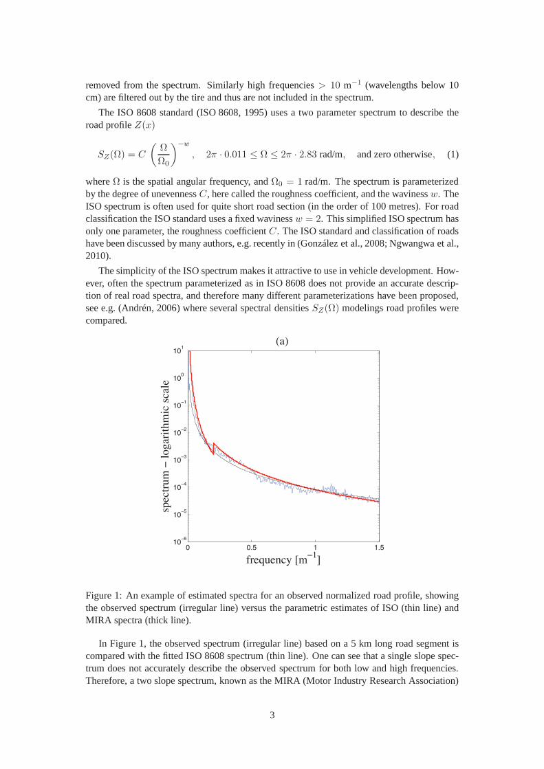
Figure 1: An example of estimated spectra for an observed normalized road profile, showingthe observed spectrum (irregular line) versus the parametric estimates of ISO (thin line) andMIRA spectra (thick line).

In Figure 1, the observed spectrum (irregular line) based ona 5 km long road segment iscompared with the fitted ISO 8608 spectrum (thin line). One can see that a single slope spec-trum does not accurately describe the observed spectrum forboth low and high frequencies.Therefore, a two slope spectrum, known as the MIRA (Motor Industry Research Association)

3

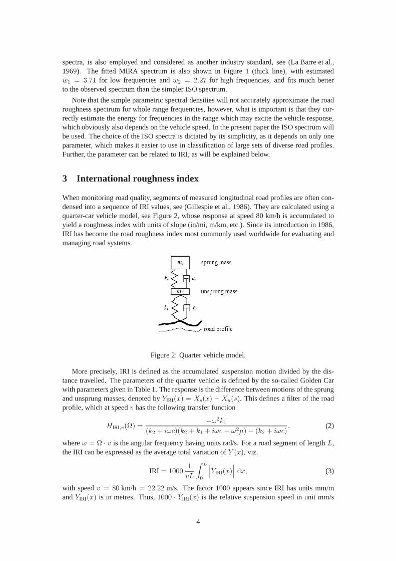
spectra, is also employed and considered as another industry standard, see (La Barre et al.,1969). The fitted MIRA spectrum is also shown in Figure 1 (thick line), with estimatedw1 = 3.71 for low frequencies andw2 = 2.27 for high frequencies, and fits much betterto the observed spectrum than the simpler ISO spectrum.

Note that the simple parametric spectral densities will notaccurately approximate the roadroughness spectrum for whole range frequencies, however, what is important is that they cor-rectly estimate the energy for frequencies in the range which may excite the vehicle response,which obviously also depends on the vehicle speed. In the present paper the ISO spectrum willbe used. The choice of the ISO spectra is dictated by its simplicity, as it depends on only oneparameter, which makes it easier to use in classification of large sets of diverse road profiles.Further, the parameter can be related to IRI, as will be explained below.

3 International roughness index

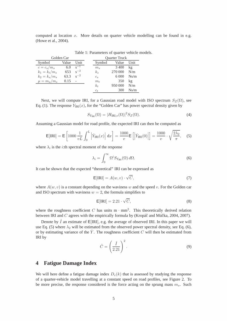
When monitoring road quality, segments of measured longitudinal road profiles are often con-densed into a sequence of IRI values, see (Gillespie et al., 1986). They are calculated using aquarter-car vehicle model, see Figure 2, whose response at speed 80 km/h is accumulated toyield a roughness index with units of slope (in/mi, m/km, etc.). Since its introduction in 1986,IRI has become the road roughness index most commonly used worldwide for evaluating andmanaging road systems.

Figure 2: Quarter vehicle model.

More precisely, IRI is defined as the accumulated suspensionmotion divided by the dis-tance travelled. The parameters of the quarter vehicle is defined by the so-called Golden Carwith parameters given in Table 1. The response is the difference between motions of the sprungand unsprung masses, denoted byYIRI(x) = Xs(x) −Xu(s). This defines a filter of the roadprofile, which at speedv has the following transfer function

HIRI,v(Ω) =−ω2k1

(k2 + iωc)(k2 + k1 + iωc− ω2µ)− (k2 + iωc), (2)

whereω = Ω · v is the angular frequency having units rad/s. For a road segment of lengthL,the IRI can be expressed as the average total variation ofY (x), viz.

IRI = 10001

vL

∫ L

0

∣

∣

∣YIRI(x)

∣

∣

∣dx, (3)

with speedv = 80 km/h = 22.22 m/s. The factor 1000 appears since IRI has units mm/mandYIRI(x) is in metres. Thus,1000 · YIRI(x) is the relative suspension speed in unit mm/s

4

computed at locationx. More details on quarter vehicle modelling can be found in e.g.(Howe et al., 2004).

Table 1: Parameters of quarter vehicle models.Golden Car

Symbol Value Unitc = cs/ms 6.0 s−1

k1 = kt/ms 653 s−2

k2 = ks/ms 63.3 s−2

µ = mu/ms 0.15 -

Quarter TruckSymbol Value Unitms 3 400 kgks 270 000 N/mcs 6 000 Ns/mmt 350 kgkt 950 000 N/mct 300 Ns/m

Next, we will compute IRI, for a Gaussian road model with ISO spectrumSZ(Ω), seeEq. (1). The responseYIRI(x), for the “Golden Car” has power spectral density given by

SYIRI (Ω) = |HIRI,v(Ω)|2SZ(Ω). (4)

Assuming a Gaussian model for road profile, the expected IRI can then be computed as

E[IRI] = E[

10001

vL

∫ L

0

∣

∣

∣YIRI(x)

∣

∣

∣dx

]

=1000

vE[∣

∣

∣YIRI(0)

∣

∣

∣

]

=1000

v·√

2λ2

π, (5)

whereλi is thei:th spectral moment of the response

λi =

∫ ∞

0

ΩiSYIRI (Ω) dΩ. (6)

It can be shown that the expected “theoretical” IRI can be expressed as

E[IRI] = A(w, v) ·√C, (7)

whereA(w, v) is a constant depending on the wavinessw and the speedv. For the Golden carand ISO spectrum with wavinessw = 2, the formula simplifies to

E[IRI] = 2.21 ·√C, (8)

where the roughness coefficientC has units m· mm2. This theoretically derived relationbetween IRI andC agrees with the empirically formula by (Kropác and Múcka, 2004, 2007).

Denote byI an estimate ofE[IRI], e.g. the average of observed IRI. In this paper we willuse Eq. (5) whereλ2 will be estimated from the observed power spectral density,see Eq. (6),or by estimating variance of theY . The roughness coefficientC will then be estimated fromIRI by

C =

(

I

2.21

)2

. (9)

4 Fatigue Damage Index

We will here define a fatigue damage indexDv(k) that is assessed by studying the responseof a quarter-vehicle model travelling at a constant speed onroad profiles, see Figure 2. Tobe more precise, the response considered is the force actingon the sprung massms. Such

5

a simplification of a physical vehicle cannot be expected to predict loads exactly, but it willhighlight the most important road characteristics as far asfatigue damage accumulation isconcerned. The parameters in the model are set to mimic heavyvehicle dynamics, following(Bogsjö, 2007). Thus, the values of the parameters differ somewhat form the ones defining theGolden car, see Table 1.

Neglecting possible “jumps”, which occur when a vehicle looses contact with the roadsurface, the response of the quarter-vehicle, i.e. the force Y (x) = msXs(x), as a function ofvehicle locationx, can be computed through linear filtering of the road profile.The filter atspeedv has the following transfer function

Hv(Ω) =msω

2(kt + iωct)

kt −(ks + iωcs)ω

2ms

−msω2 + ks + iωcs−mtω2 + iωct

(

1 +msω

2

ks −msω2 + iωcs

)

, (10)

whereω = Ω · v is the angular frequency having units rad/s.

For a stationary road modelZ(x) having power spectral densitySZ(Ω), the responseY (x),for a vehicle at speedv [m/s], has power spectral density given by

SY (Ω) = |Hv(Ω)|2SZ(Ω), SZ(Ω) = σ2S0 (Ω) , (11)

whereσ2 =∫∞

−∞SZ(Ω) dΩ. Note thatσ2 is a variance of the road profile model and it may

not be equal to the measured road profile variance, e.g. whenSZ(Ω) is ISO spectrum.

In general the responseY (x), which is the force acting on the sprung mass, is computedby means of filtering the signalZ(x) using the filter with transfer functionHv(Ω) given inEq. (10), which depends on the vehicle speedv. In the examplev = 10, 15 [m/s] have beenused. The response of the quarter vehicleY (x) is the solution of a fourth order ordinarydifferential equation or alternatively a convolution ofZ(x) with the vehicle’s impulse responsehv(x), viz.

Y (x) =

∫ x

−∞

hv(x− u)Z(u)du. (12)

In this paper responses for measured and simulated roads arecomputed using the FFT algo-rithm. Since the initial conditions of the system att = 0 are unknown the Hanning windowhas been used to make the start and the end of the ride smooth. This is necessary or otherwisethe first oscillation of the response may cause all the damage– the car is hitting a wall.

The purpose of this work is to propose models forZ(x) defined by means of few parametersthat could be used to computeY (x) or other more complex and realistic responses in such away that the risk for fatigue failure, or extremal responses, could be quantified. Hence the mostimportant criterion for a good model of a measured road profile is that the rainflow damage ofthe response is well represented.

The rainflow damage is computed in two steps. First rainflow ranges∆Srfc,i in the loadY (x), 0 ≤ x ≤ Lp, are found, then the rainflow damage per metre is computed according toPalmgren-Miner rule (Palmgren, 1924; Miner, 1945), viz.

Dv(k) =1

Lp

∑

i

∆Skrfc,i, (13)

see also (Rychlik, 1987) for details of this approach. In this paper2 ≤ k ≤ 5, have beenused. The damageDv(k) for higher exponent valuek = 5 depends mostly on the proportionand size of large cycles, while damage fork = 3, corresponding to the crack growth process,

6

depends on the sizes of both large and moderately large cycles. For a stationary load,Dv(k)converges to a limit asLp increases without bounds. However, for short road profiles,Dv(k)may vary considerably. For ergodic loads the limit is equal to the expected damageE[Dv(k)].In Section 6, computations of the expected damage will be further discussed. In these compu-tations, the response to the normalized road profileZ(x) having the spectrumS0(Ω) will beemployed, viz.

Y (x) =

∫ x

−∞

hv(x− u)Z(u)du. (14)

The spectrum ofY (x) is given by

SY (Ω) = |Hv(Ω)|2S0(Ω). (15)

5 Stochastic models for road profiles

Parts of this section follows (Bogsjö et al., 2012). First, the commonly used stationary Gaus-sian model will be presented. Then, in Section 5.2, we introduce the non-stationary Gaussianmodel with variable variances between short sections, but with smooth transitions between thesegments, and then extend it to the non-stationary Laplace model where the variable varianceis modelled by a Gamma distribution. Recall that, for a road profile Z(x) with standard devi-ationσ, we denote byZ(x) the normalized profile, i.e.E[Z(x)] = 0 andV[Z(x)] = 1. Thus,for a zero mean profile,Z(x) = σZ(x) with spectrumSZ(Ω) = σ2S0(Ω), whereS0(Ω) isthe spectrum of the normalized road profileZ(x)

In the following sections we will discuss Laplace models with ISO spectrum and givemeans to estimate parameters in the model from an observed IRI sequence. Note that the IRIis often available in road maintenance databases. MATLAB code to simulate the road modelsis given in Appendix B.

5.1 Stationary Gaussian model

A zero mean stationary Gaussian process is completely defined by its mean and power spec-trum, thus, any probability statement about properties of Gaussian processes can in principlebe expressed by means of the spectrum. This is not always practically possible and henceMonte Carlo methods are often employed. There are several ways to generate Gaussian sam-ple paths. The algorithm proposed in (Shinozuka, 1971) is often used in engineering. It isbased on the spectral representation of a stationary process. Here we use an alternative waythat expresses a Gaussian process as a moving average of white noise.

Roughly speaking a moving average process is a convolution of a kernel functiong(x), say,with a infinitesimal “white noise” process having variance equal to the spatial discretizationstep, say dx. Consider a kernel functiong(x), which is normalized so that its square integratesto one. Then the standardized Gaussian process can be approximated by

Z(x) ≈∑

g(x− xi)Zi

√dx, (16)

where theZi’s are independent standard Gaussian random variables, while dx is the discretiza-tion step, here reciprocal of the sampling frequency (dx = 5 cm). An appropriate choice ofthe length of the increment dx is related to smoothness of the kernel.

In order to get a Gaussian process with a desired spectral density one has to use an appro-priate kernelg(x). Consider a symmetric kernel, i.e.g(−x) = g(x). In this case, the spectrum

7

S0(Ω) of Z(x) uniquely defines the kernelg(x) since

S0(Ω) =1

2π|Fg(Ω)|2, (17)

whereFg(Ω) stands for the Fourier transform, and for symmetric kernelstheir Fourier trans-form is given by

Fg(Ω) =√

2π S0(Ω). (18)

5.2 Non-stationary models

Stationary Gaussian loads have been extensively studied inliterature and applied as modelsfor road roughness, see e.g. (Dodds and Robson, 1973) for an early application. However,the authors of that paper were aware that Gaussian processescannot “exactly reproduce theprofile of a real road”. In (Charles, 1993) a non-stationary model was proposed, constructedas a sequence of independent Gaussian processes of varying standard deviations but the samestandardized spectrumS0(Ω). Knowing durations and sizes of standard deviations the modelis a non-stationary Gaussian process. Similar approaches were used in (Bruscella et al., 1999;Rouillard, 2004, 2009). The variability of the standard deviationσ was modelled by a discretedistribution taking a few number of values (in published work the number of values was six).In (Rouillard, 2009) random lengths of constant variance sections were also considered. Inthose papers one was not concerned with the problem of connecting the segments with con-stant variances into one signal since the response was modelled as a non-stationary Gaussianprocess, i.e. by a process of the same type as the model of the road surface. Such individualtreatment of the constant variance segments is possible only if they are much longer than thesupport of the kernelg(x), e.g. in the order of kilometres. However, actual roads contain muchshorter sections with above-average irregularity. These irregularities cause most of the vehiclefatigue damage, as reported in (Bogsjö, 2007).

Since we are dealing with non-stationary models it is not obvious how the normalized roadprofile Z(x) should be defined. Here we will assume thatZ(x), x ∈ [0, Lp] has mean zero andvariance one, which means that the mean and variance ofZ(x) at a pointx chosen at randomfrom [0, Lp] are zero and one, respectively.

For example suppose that the normalized road profileZ(x), x ∈ [0, L], consists ofMequally long segments of lengthL = Lp/M , where the constant variance of thej:th segmentis equal torj, j = 1, . . . ,M with 1

M

∑Mj=1

rj = 1 sinceZ(x) has variance one. However,such a process is discontinuous at times where the variance is changing. Although formallycorrect, the model induces a transient largely contributing to the fatigue damage each time avehicle passes these locations. A more realistic approach can be made by continuous tran-sitions between segments of constant variance. This can be done in different ways but herewe employ moving averages of "non-stationary" white noise to define a smooth version ofZ(x). First we present the non-stationary Gaussian model with variable variances but smoothtransitions between the segments, and then extend it to the non-stationary Laplace model.

5.3 Non-stationary Gaussian model

The process consists ofM segments of lengthL = Lp/M and we wish to define a processon [0, Lp]. We would like that each segment has a prescribed standard deviation σj , j =

1, . . . ,M . Obviously the variance of the process isσ2 = 1

M

∑Mj=1

σ2

j .

8

Denote the standardized variance of thej:th segment by

rj = σ2

j/σ2. (19)

Next we will define thej:th non-stationary Gaussian processZj(x) process for all0 ≤ x ≤Lp. Let again dx be the sampling step of the process and[sj−1, sj ], sj−sj−1 = L, the intervalwhere the road profile model would have the varianceσ2

j , viz. s0 = 0 < s1 < . . . < sM = Lp.

Now defineM processesZj(x) as follows

Zj(x) ≈∑

sj−1<xi≤sj

g(x − xi)√rj Zi

√dx, (20)

where theZi’s are independent standard Gaussian variables, and dx is the discretization step.Finally the road profile modelZ(x) is given by

Z(x) = σZ(x) = σM∑

j=1

Zj(x). (21)

5.4 Non-stationary Laplace model

A reasonable length of road segments with constant varianceis 200 metres. This would meanthat in order to describe a 10 km long road with ISO spectrum one would need 50σ2

j param-eters. This is not very convenient and therefore in (Bogsjö et al., 2012) another approach wastaken. Namely, the variability of the standardized variancesrj, defined in Eq. (19), was mod-elled by means of the Gamma probability distribution, i.e.rj are independent observations ofa random variableR having probability distribution function

fR(r) =θθ

Γ(θ)rθ−1 exp(−rθ). (22)

By replacingrj in Eq. (20) by independent Gamma random variablesRj , we get

Zj(x) ≈∑

sj−1<xi≤sj

g(x− xi)√

Rj Zi

√dx. (23)

and the road profileZ(x) is given by

Z(x) = σZ(x) = σ

M∑

j=1

Zj(x). (24)

Further, for a zero mean Gaussian random variableZj, the product√

RjZj has a Laplacedistribution, and thus the processZ(x), defined in Eq. (24), has a generalized Laplace distri-bution, see (Kotz et al., 2001). MATLAB code to simulate thismodel can be found in Ap-pendix B.

It should be noted that a non-stationary Laplace road model requires only two parameters;the varianceσ2 of the process and the shape parameterθ of the Gamma distribution. In Laplacemodelling, traditionally another parameterization is used, viz. ν = 1/θ. Now if the shapeparameterν is close to zero then the Laplace process is close to be a Gaussian process. Theshape parameterν of the Laplace process can also be computed from the kurtosisκ of theprocessZ(x), namely

ν = (κ− 3)/3. (25)

9

Alternatively, if the variances of the road segments with constant variance are known, thenthe moment method gives the following estimates

σ2 =1

M

M∑

j=1

σ2

j , ν =1

M−1

∑Mj=1

(σ2

j − σ2)2

(σ2)2. (26)

5.5 Road models with ISO spectrum

The kernelg(x) defined by the ISO spectrum, which in the standardized form (variance oneand wavinessw = 2) is given by

S0(Ω) = C0

(

Ω

Ω0

)−2

, C0 = 14.4 m3, 2π · 0.011 ≤ Ω ≤ 2π · 2.83 rad/m, (27)

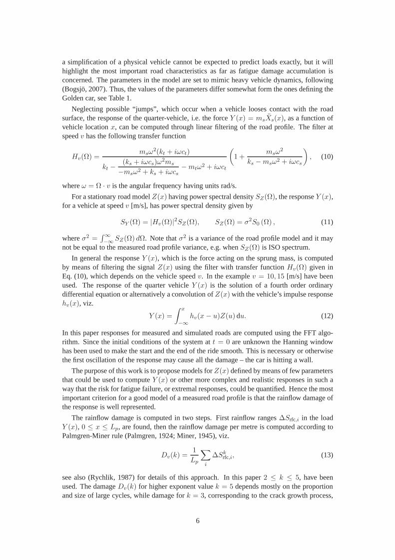
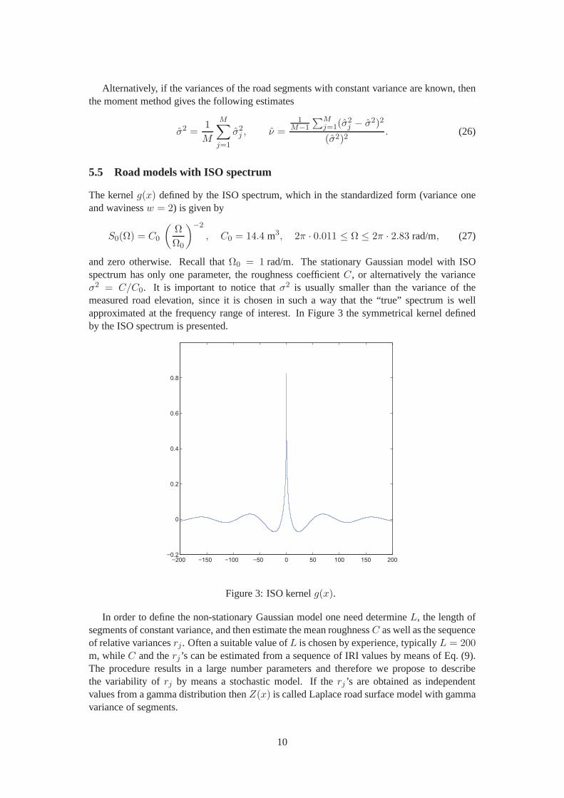
and zero otherwise. Recall thatΩ0 = 1 rad/m. The stationary Gaussian model with ISOspectrum has only one parameter, the roughness coefficientC, or alternatively the varianceσ2 = C/C0. It is important to notice thatσ2 is usually smaller than the variance of themeasured road elevation, since it is chosen in such a way thatthe “true” spectrum is wellapproximated at the frequency range of interest. In Figure 3the symmetrical kernel definedby the ISO spectrum is presented.

−200 −150 −100 −50 0 50 100 150 200−0.2

0

0.2

0.4

0.6

0.8

Figure 3: ISO kernelg(x).

In order to define the non-stationary Gaussian model one needdetermineL, the length ofsegments of constant variance, and then estimate the mean roughnessC as well as the sequenceof relative variancesrj. Often a suitable value ofL is chosen by experience, typicallyL = 200m, whileC and therj ’s can be estimated from a sequence of IRI values by means of Eq. (9).The procedure results in a large number parameters and therefore we propose to describethe variability of rj by means a stochastic model. If therj ’s are obtained as independentvalues from a gamma distribution thenZ(x) is called Laplace road surface model with gammavariance of segments.

10

In order to define the Laplace model with ISO spectrum, we needtwo parameters, themean roughnessC and the Laplace shape parameterν, modelling the gamma variances for thesegments of lengthL. Consequently, by introducing one additional parameterν, the station-ary Gaussian model is extended to the non-stationary Laplace model. Recall that setting theparameterν equal zero gives the stationary Gaussian case.

5.6 Estimation of Laplace road models with ISO spectrum

How to estimate the parameters in a Laplace, or a Gaussian model, with ISO spectrum is notobvious and many possible approaches are possible. The difficulty lies in the fact that an“useful” ISO model has varianceσ2 and kurtosisκ that differ from the variance and kurtosisestimated from measured road profile. Consequently, relations (25-26) andC = σ2C0 are noappropriate estimators whenσ2

j are estimated variances from measured road profiles.

However, Eq. (26) is still useful if theσ2

j ’s are replaced by roughness coefficientsCj ’s,defining ISO spectra, for short road segments. The roughnesscoefficientsCj could be esti-mated by means of some statistical procedure if the measuredprofile is available. However,this is seldom the case, and hence we will propose to estimateCj from a sequence of IRI val-ues using Eq. (8). Note that IRI parameters are often available from road databases maintainedby road agencies.

Summarizing, we propose to estimateCj by

Cj =

(

Ij2.21

)2

, (28)

whereIj is an estimate of IRI of thej:th segment, see Eq. (3). Having a sequence of estimatesCj, j = 1, . . . ,M , it is possible to estimateC by the average ofCj . Next, sinceCj is pro-portional to the varianceσ2

j , for Z(x) with ISO spectrum, one can also useCj/C as estimatesof rj and, for example, the maximum likelihood method can be used to estimate the shapeparameterν. However, for simplicity of presentation, the moment method will be employedhere, giving the following estimates

C =1

M

M∑

j=1

Cj, ν =1

M−1

∑Mj=1

(Cj − C)2

C2. (29)

6 Expected damage index

The purpose of this section is to present a closed form approximation for the expected dam-age index for the Laplace road profile model with ISO spectrum. The important special caseof Gaussian response,ν = 0, have been intensively studied in the literature and many ap-proximations are available, see (Bengtsson and Rychlik, 2009) for comparisons of differentapproaches. Therefore, we wish to relate the expected damage index for the Laplace model tothe expected Gaussian index.

For the Gaussian model, the damage indexDv(k), defined in Eq. (13), depends on thefollowing parameters; the speedv, the exponentk in the S-N curve, the road roughness coef-ficientC, see Eqs. (11) and (27) for ISO spectrum. For the Laplace model, the damage indexdepends additionally on the shape parameterν. In order to make the dependence explicit inthe notation we will writeDv(k,C, ν) for Dv(k).

11

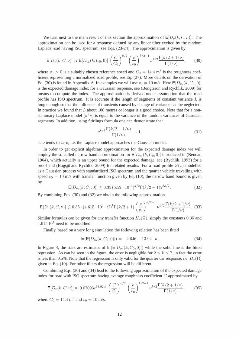
We turn next to the main result of this section the approximation of E[Dv(k,C, ν)]. Theapproximation can be used for a response defined by any linearfilter excited by the randomLaplace road having ISO spectrum, see Eqs. (23-24). The approximation is given by

E[Dv(k,C, ν)] ≈ E[Dv0(k,C0, 0)]

(

C

C0

)k/2( v

v0

)k/2−1

νk/2Γ(k/2 + 1/ν)

Γ(1/ν), (30)

wherev0 > 0 is a suitably chosen reference speed andC0 = 14.4 m3 is the roughness coef-ficient representing a normalized road profile, see Eq. (27).More details on the derivation ofEq. (30) is found in Appendix A. In examples we will usev0 = 10 m/s. HereE[Dv0(k,C0, 0)]is the expected damage index for a Gaussian response, see (Bengtsson and Rychlik, 2009) formeans to compute the index. The approximation is derived under assumption that the roadprofile has ISO spectrum. It is accurate if the length of segments of constant varianceL islong enough so that the influence of transients caused by change of variance can be neglected.In practice we found thatL about 100 metres or longer is a good choice. Note that for a non-stationary Laplace model(σ2ν) is equal to the variance of the random variances of Gaussiansegments. In addition, using Stirlings formula one can demonstrate that

νk/2Γ(k/2 + 1/ν)

Γ(1/ν)→ 1, (31)

asν tends to zero, i.e. the Laplace model approaches the Gaussian model.

In order to get explicit algebraic approximation for the expected damage index we willemploy the so-called narrow band approximation forE[Dv0(k,C0, 0)] introduced in (Bendat,1964), which actually is an upper bound for the expected damage, see (Rychlik, 1993) for aproof and (Bogsjö and Rychlik, 2009) for related results. For a road profileZ(x) modelledas a Gaussian process with standardized ISO spectrum and thequarter vehicle travelling withspeedv0 = 10 m/s with transfer function given by Eq. (10), the narrow bandbound is givenby

E[Dv0(k,C0, 0)] ≤ 0.35 (5.52 · 1010)k/2Γ(k/2 + 1)23k/2. (32)

By combining Eqs. (30) and (32) we obtain the following approximation

E[Dv(k,C, ν)] . 0.35 · (4.615 · 104 ·C)kΓ(k/2 + 1)

(

v

v0

)k/2−1

νk/2Γ(k/2 + 1/ν)

Γ(1/ν). (33)

Similar formulas can be given for any transfer functionHv(Ω), simply the constants0.35 and4.615 104 need to be modified.

Finally, based on a very long simulation the following relation has been fitted

ln(E[Dv0(k,C0, 0)]) = −2.646 + 13.92 · k. (34)

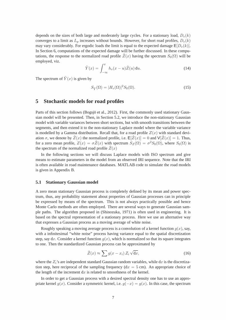
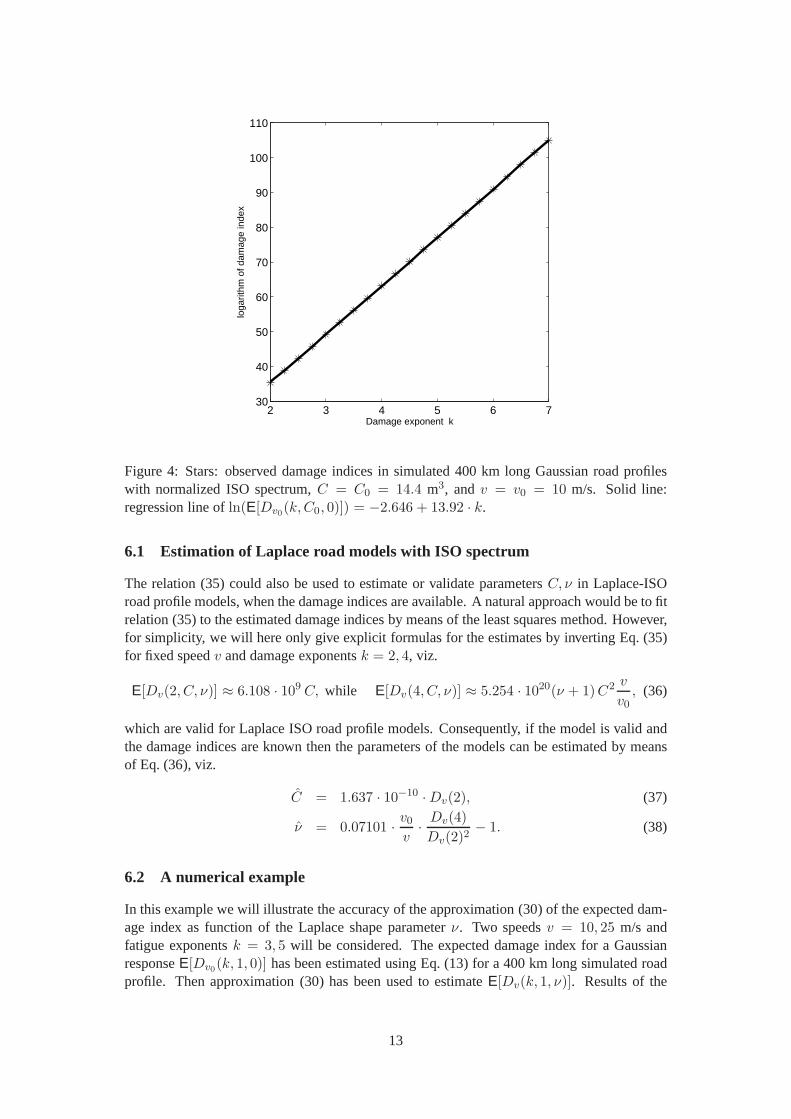
In Figure 4, the stars are estimates ofln(E[Dv0(k,C0, 0)]) while the solid line is the fittedregression. As can be seen in the figure, the error is negligible for 2 ≤ k ≤ 7, in fact the erroris less than 0.5%. Note that the regression is only valid for the quarter car response, i.e.Hv(Ω)given in Eq. (10). For other filters the regression will be different.

Combining Eqs. (30) and (34) lead to the following approximation of the expected damageindex for road with ISO spectrum having average roughness coefficientC approximated by

E[Dv(k,C, ν)] ≈ 0.07093e13.92 k

(

C

C0

)k/2 ( v

v0

)k/2−1

νk/2Γ(k/2 + 1/ν)

Γ(1/ν), (35)

whereC0 = 14.4 m3 andv0 = 10 m/s.

12

2 3 4 5 6 730

40

50

60

70

80

90

100

110

Damage exponent k

loga

rithm

of d

amag

e in

dex

Figure 4: Stars: observed damage indices in simulated 400 kmlong Gaussian road profileswith normalized ISO spectrum,C = C0 = 14.4 m3, andv = v0 = 10 m/s. Solid line:regression line ofln(E[Dv0(k,C0, 0)]) = −2.646 + 13.92 · k.

6.1 Estimation of Laplace road models with ISO spectrum

The relation (35) could also be used to estimate or validate parametersC, ν in Laplace-ISOroad profile models, when the damage indices are available. Anatural approach would be to fitrelation (35) to the estimated damage indices by means of theleast squares method. However,for simplicity, we will here only give explicit formulas forthe estimates by inverting Eq. (35)for fixed speedv and damage exponentsk = 2, 4, viz.

E[Dv(2, C, ν)] ≈ 6.108 · 109 C, while E[Dv(4, C, ν)] ≈ 5.254 · 1020(ν + 1)C2v

v0, (36)

which are valid for Laplace ISO road profile models. Consequently, if the model is valid andthe damage indices are known then the parameters of the models can be estimated by meansof Eq. (36), viz.

C = 1.637 · 10−10 ·Dv(2), (37)

ν = 0.07101 · v0v

· Dv(4)

Dv(2)2− 1. (38)

6.2 A numerical example

In this example we will illustrate the accuracy of the approximation (30) of the expected dam-age index as function of the Laplace shape parameterν. Two speedsv = 10, 25 m/s andfatigue exponentsk = 3, 5 will be considered. The expected damage index for a GaussianresponseE[Dv0(k, 1, 0)] has been estimated using Eq. (13) for a 400 km long simulated roadprofile. Then approximation (30) has been used to estimateE[Dv(k, 1, ν)]. Results of the

13

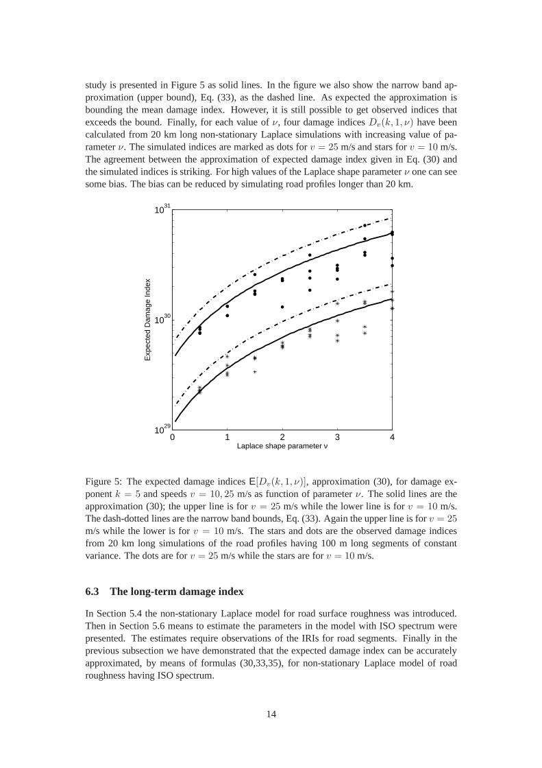
study is presented in Figure 5 as solid lines. In the figure we also show the narrow band ap-proximation (upper bound), Eq. (33), as the dashed line. As expected the approximation isbounding the mean damage index. However, it is still possible to get observed indices thatexceeds the bound. Finally, for each value ofν, four damage indicesDv(k, 1, ν) have beencalculated from 20 km long non-stationary Laplace simulations with increasing value of pa-rameterν. The simulated indices are marked as dots forv = 25 m/s and stars forv = 10 m/s.The agreement between the approximation of expected damageindex given in Eq. (30) andthe simulated indices is striking. For high values of the Laplace shape parameterν one can seesome bias. The bias can be reduced by simulating road profileslonger than 20 km.

0 1 2 3 410

29

1030

1031

Laplace shape parameter ν

Exp

ecte

d D

amag

e In

dex

Figure 5: The expected damage indicesE[Dv(k, 1, ν)], approximation (30), for damage ex-ponentk = 5 and speedsv = 10, 25 m/s as function of parameterν. The solid lines are theapproximation (30); the upper line is forv = 25 m/s while the lower line is forv = 10 m/s.The dash-dotted lines are the narrow band bounds, Eq. (33). Again the upper line is forv = 25m/s while the lower is forv = 10 m/s. The stars and dots are the observed damage indicesfrom 20 km long simulations of the road profiles having 100 m long segments of constantvariance. The dots are forv = 25 m/s while the stars are forv = 10 m/s.

6.3 The long-term damage index

In Section 5.4 the non-stationary Laplace model for road surface roughness was introduced.Then in Section 5.6 means to estimate the parameters in the model with ISO spectrum werepresented. The estimates require observations of the IRIs for road segments. Finally in theprevious subsection we have demonstrated that the expecteddamage index can be accuratelyapproximated, by means of formulas (30,33,35), for non-stationary Laplace model of roadroughness having ISO spectrum.

14

Since Eqs. (35) and (33) are given by explicit algebraic functions of model parametersthese are very convenient for estimation of the long-term damage accumulation in a vehiclecomponent. If the variability of parametersσ2; the shape parameterν in Laplace model andv driving speed for a population of customers or a market is known and if the response canbe described by means of a linear filter with an appropriate transfer functionH (here approx-imated by the quarter vehicleHv, Eq. (10)), then the expected long-term damage indexE[D]can be approximated by means of the following integral

E[D] ≈ dk

∫(∫

vk/2−1f(v|ν, σ) dv)

· (ν · σ2)k/2Γ(k/2 + 1/ν)

Γ(1/ν)f(ν, σ) dσ dν. (39)

with the damage growth intensitydk = E[Dv0(k, 1, 0)]/vk/2−1

0, see Eq. (42) in Appendix A, is

easily available, see (Bengtsson and Rychlik, 2009). The density f(ν, σ) characterizes the en-countered road quality, while the conditional densityf(v|ν, σ) represents the driver behaviour.

7 Validation of the Laplace-ISO model of road profiles

A remaining important question is how well the Laplace-ISO model fits measured road pro-files. In this section we shall validate the Laplace-ISO roadprofile model by studying thefollowing issues:

1) Can the non-stationary Laplace model be used to reconstruct road profiles?

2) Can the ISO spectrum give sufficiently accurate approximations of road profiles?

3) Can the IRI be used to estimate the ISO spectrum?

4) What is the suitable length of segments with constant variance?

For the validation a data set of eight sections of roads with measured road profiles will be used.The eight selected sections represent different types of roads as well as different geographi-cal locations. The lengths of the sections varies between 14and 45 kilometres, see Table 2second row. The measurements have been provided by Scania and were standardized to havezero mean and variance one. The signals are then filtered so that the low frequencies, withwavelength above 100 metres are removed. In the following the road profile will always meanthe filtered road profile. The third row in the table contains estimates of standard deviations ofthe filtered signals, while the fourth row their kurtosis. One can see that the estimates of thekurtosis are significantly higher than 3 implying that road profiles should not be modelled as astationary Gaussian processes.

The accuracy of the model will be validated by means of relative indices, i.e. fractionsof the damage indices derived from a model and the observed indices, for various values ofparameters the speedv the damage exponentk and lengthL of constant variance segments. Arelative index equal to one means that the damage index computed for the model is equal tothe observed index in the measured profile.

7.1 Laplace model with observed spectra

In this section we demonstrate that the general non-stationary Laplace model can be used todescribe the variability of the eight measured road profiles. In the model symmetrical kernelsg are used, which are estimated using Eq. (18) whereS0(Ω) is replaced by empirical spectra.

15

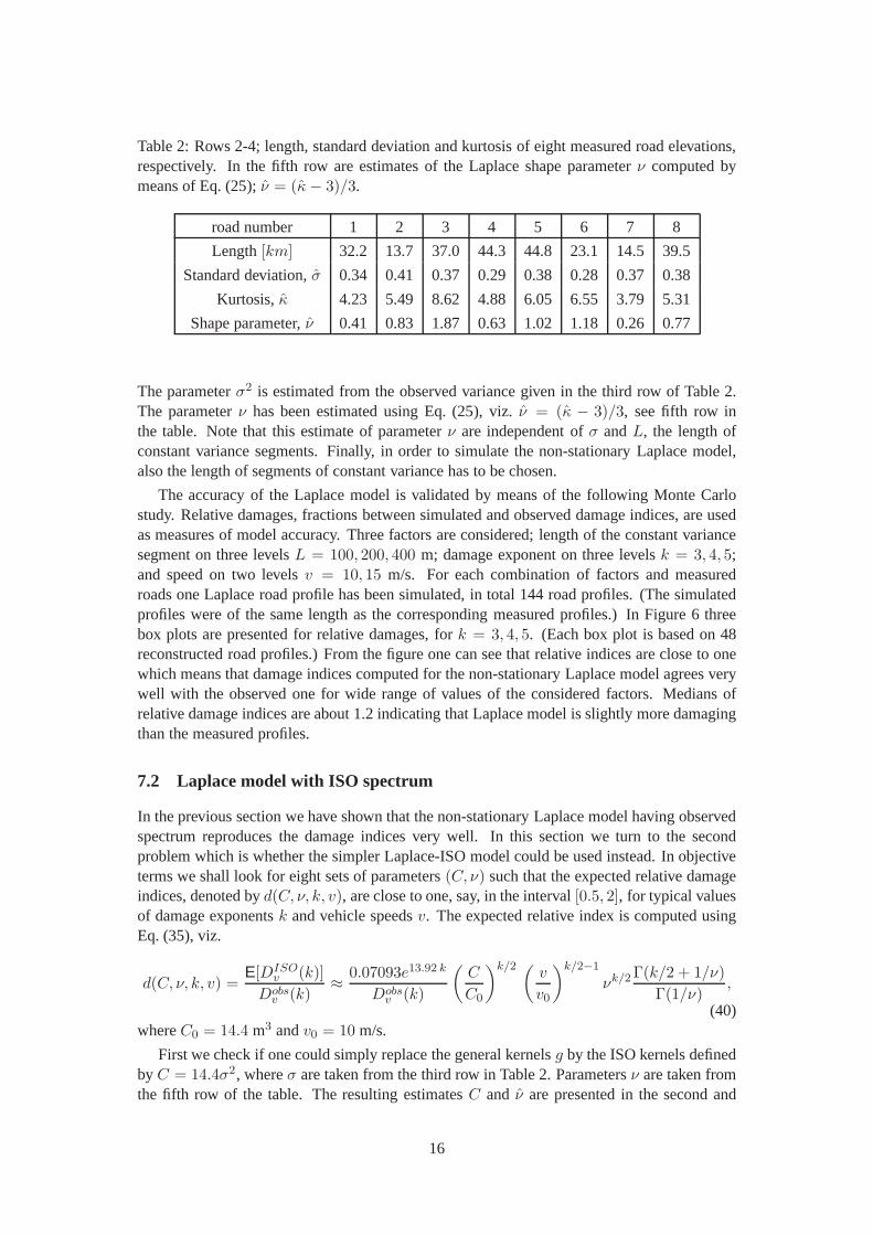
Table 2: Rows 2-4; length, standard deviation and kurtosis of eight measured road elevations,respectively. In the fifth row are estimates of the Laplace shape parameterν computed bymeans of Eq. (25);ν = (κ− 3)/3.

road number 1 2 3 4 5 6 7 8

Length[km] 32.2 13.7 37.0 44.3 44.8 23.1 14.5 39.5

Standard deviation,σ 0.34 0.41 0.37 0.29 0.38 0.28 0.37 0.38

Kurtosis,κ 4.23 5.49 8.62 4.88 6.05 6.55 3.79 5.31

Shape parameter,ν 0.41 0.83 1.87 0.63 1.02 1.18 0.26 0.77

The parameterσ2 is estimated from the observed variance given in the third row of Table 2.The parameterν has been estimated using Eq. (25), viz.ν = (κ − 3)/3, see fifth row inthe table. Note that this estimate of parameterν are independent ofσ andL, the length ofconstant variance segments. Finally, in order to simulate the non-stationary Laplace model,also the length of segments of constant variance has to be chosen.

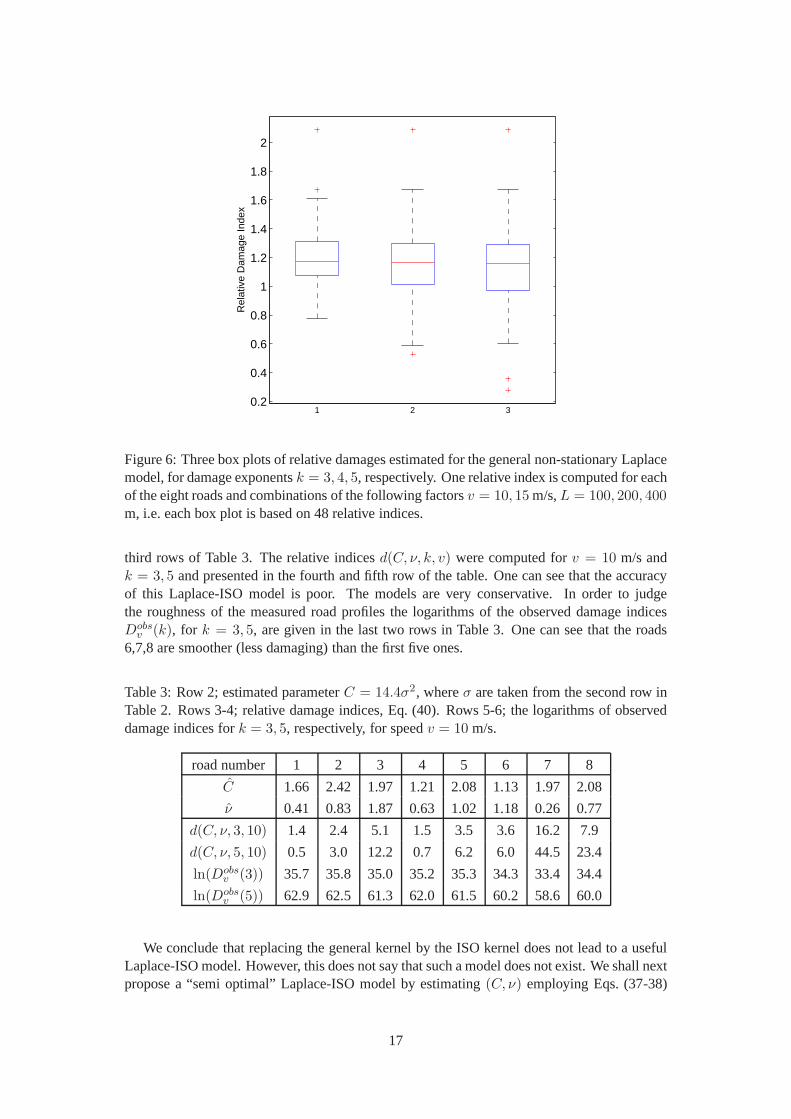
The accuracy of the Laplace model is validated by means of thefollowing Monte Carlostudy. Relative damages, fractions between simulated and observed damage indices, are usedas measures of model accuracy. Three factors are considered; length of the constant variancesegment on three levelsL = 100, 200, 400 m; damage exponent on three levelsk = 3, 4, 5;and speed on two levelsv = 10, 15 m/s. For each combination of factors and measuredroads one Laplace road profile has been simulated, in total 144 road profiles. (The simulatedprofiles were of the same length as the corresponding measured profiles.) In Figure 6 threebox plots are presented for relative damages, fork = 3, 4, 5. (Each box plot is based on 48reconstructed road profiles.) From the figure one can see thatrelative indices are close to onewhich means that damage indices computed for the non-stationary Laplace model agrees verywell with the observed one for wide range of values of the considered factors. Medians ofrelative damage indices are about 1.2 indicating that Laplace model is slightly more damagingthan the measured profiles.

7.2 Laplace model with ISO spectrum

In the previous section we have shown that the non-stationary Laplace model having observedspectrum reproduces the damage indices very well. In this section we turn to the secondproblem which is whether the simpler Laplace-ISO model could be used instead. In objectiveterms we shall look for eight sets of parameters(C, ν) such that the expected relative damageindices, denoted byd(C, ν, k, v), are close to one, say, in the interval[0.5, 2], for typical valuesof damage exponentsk and vehicle speedsv. The expected relative index is computed usingEq. (35), viz.

d(C, ν, k, v) =E[DISO

v (k)]

Dobsv (k)

≈ 0.07093e13.92 k

Dobsv (k)

(

C

C0

)k/2 ( v

v0

)k/2−1

νk/2Γ(k/2 + 1/ν)

Γ(1/ν),

(40)whereC0 = 14.4 m3 andv0 = 10 m/s.

First we check if one could simply replace the general kernels g by the ISO kernels definedbyC = 14.4σ2, whereσ are taken from the third row in Table 2. Parametersν are taken fromthe fifth row of the table. The resulting estimatesC and ν are presented in the second and

16

0.2

0.4

0.6

0.8

1

1.2

1.4

1.6

1.8

2

1 2 3

Rel

ativ

e D

amag

e In

dex

Figure 6: Three box plots of relative damages estimated for the general non-stationary Laplacemodel, for damage exponentsk = 3, 4, 5, respectively. One relative index is computed for eachof the eight roads and combinations of the following factorsv = 10, 15 m/s,L = 100, 200, 400m, i.e. each box plot is based on 48 relative indices.

third rows of Table 3. The relative indicesd(C, ν, k, v) were computed forv = 10 m/s andk = 3, 5 and presented in the fourth and fifth row of the table. One can see that the accuracyof this Laplace-ISO model is poor. The models are very conservative. In order to judgethe roughness of the measured road profiles the logarithms ofthe observed damage indicesDobs

v (k), for k = 3, 5, are given in the last two rows in Table 3. One can see that the roads6,7,8 are smoother (less damaging) than the first five ones.

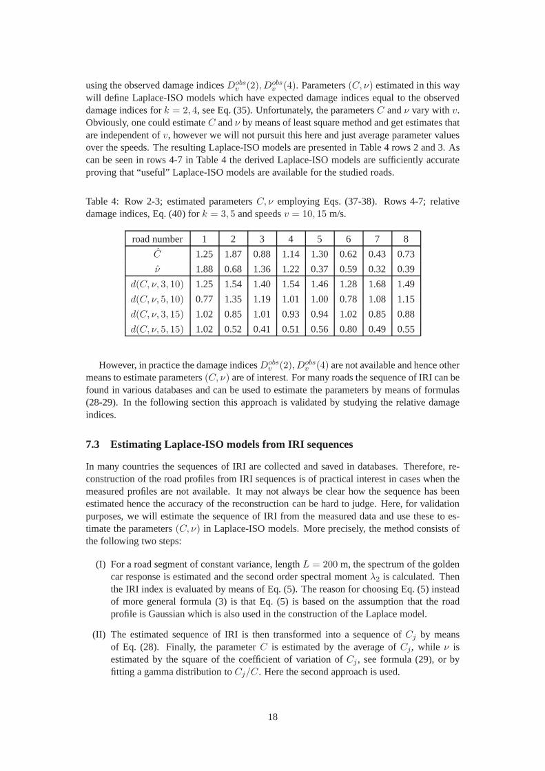
Table 3: Row 2; estimated parameterC = 14.4σ2, whereσ are taken from the second row inTable 2. Rows 3-4; relative damage indices, Eq. (40). Rows 5-6; the logarithms of observeddamage indices fork = 3, 5, respectively, for speedv = 10 m/s.

road number 1 2 3 4 5 6 7 8

C 1.66 2.42 1.97 1.21 2.08 1.13 1.97 2.08

ν 0.41 0.83 1.87 0.63 1.02 1.18 0.26 0.77

d(C, ν, 3, 10) 1.4 2.4 5.1 1.5 3.5 3.6 16.2 7.9

d(C, ν, 5, 10) 0.5 3.0 12.2 0.7 6.2 6.0 44.5 23.4

ln(Dobsv (3)) 35.7 35.8 35.0 35.2 35.3 34.3 33.4 34.4

ln(Dobsv (5)) 62.9 62.5 61.3 62.0 61.5 60.2 58.6 60.0

We conclude that replacing the general kernel by the ISO kernel does not lead to a usefulLaplace-ISO model. However, this does not say that such a model does not exist. We shall nextpropose a “semi optimal” Laplace-ISO model by estimating(C, ν) employing Eqs. (37-38)

17

using the observed damage indicesDobsv (2),Dobs

v (4). Parameters(C, ν) estimated in this waywill define Laplace-ISO models which have expected damage indices equal to the observeddamage indices fork = 2, 4, see Eq. (35). Unfortunately, the parametersC andν vary withv.Obviously, one could estimateC andν by means of least square method and get estimates thatare independent ofv, however we will not pursuit this here and just average parameter valuesover the speeds. The resulting Laplace-ISO models are presented in Table 4 rows 2 and 3. Ascan be seen in rows 4-7 in Table 4 the derived Laplace-ISO models are sufficiently accurateproving that “useful” Laplace-ISO models are available forthe studied roads.

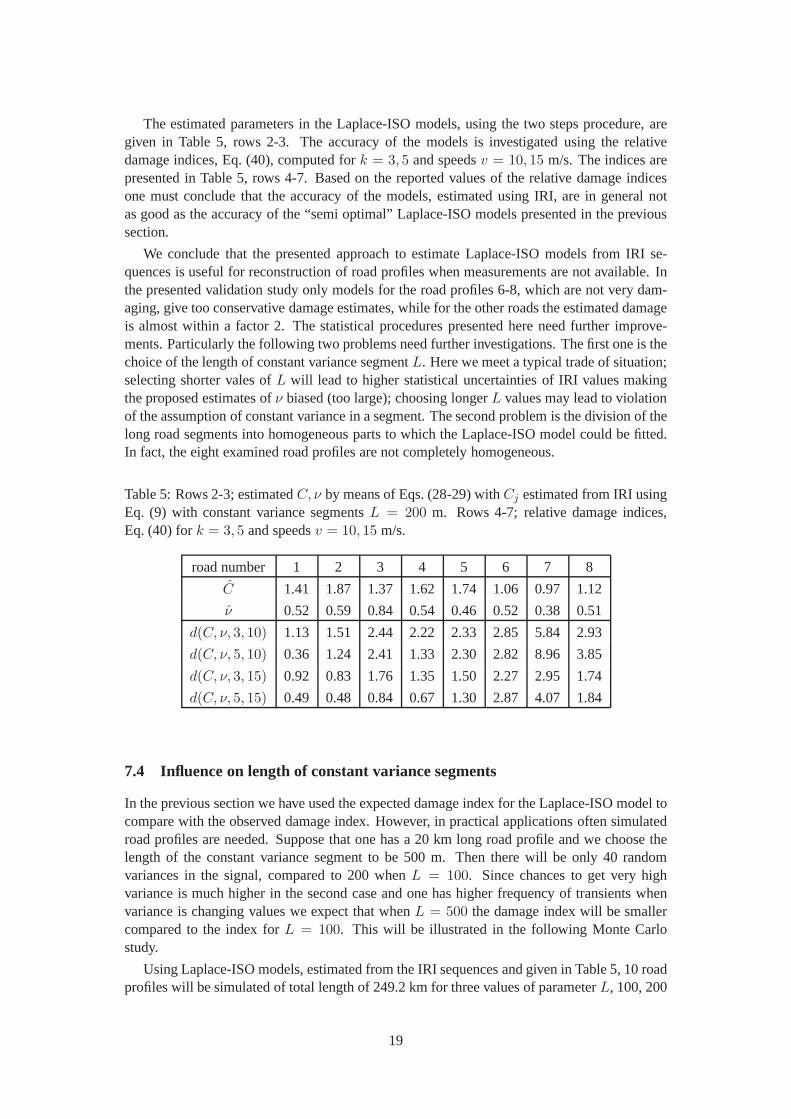
Table 4: Row 2-3; estimated parametersC, ν employing Eqs. (37-38). Rows 4-7; relativedamage indices, Eq. (40) fork = 3, 5 and speedsv = 10, 15 m/s.

road number 1 2 3 4 5 6 7 8

C 1.25 1.87 0.88 1.14 1.30 0.62 0.43 0.73

ν 1.88 0.68 1.36 1.22 0.37 0.59 0.32 0.39

d(C, ν, 3, 10) 1.25 1.54 1.40 1.54 1.46 1.28 1.68 1.49

d(C, ν, 5, 10) 0.77 1.35 1.19 1.01 1.00 0.78 1.08 1.15

d(C, ν, 3, 15) 1.02 0.85 1.01 0.93 0.94 1.02 0.85 0.88

d(C, ν, 5, 15) 1.02 0.52 0.41 0.51 0.56 0.80 0.49 0.55

However, in practice the damage indicesDobsv (2),Dobs

v (4) are not available and hence othermeans to estimate parameters(C, ν) are of interest. For many roads the sequence of IRI can befound in various databases and can be used to estimate the parameters by means of formulas(28-29). In the following section this approach is validated by studying the relative damageindices.

7.3 Estimating Laplace-ISO models from IRI sequences

In many countries the sequences of IRI are collected and saved in databases. Therefore, re-construction of the road profiles from IRI sequences is of practical interest in cases when themeasured profiles are not available. It may not always be clear how the sequence has beenestimated hence the accuracy of the reconstruction can be hard to judge. Here, for validationpurposes, we will estimate the sequence of IRI from the measured data and use these to es-timate the parameters(C, ν) in Laplace-ISO models. More precisely, the method consistsofthe following two steps:

(I) For a road segment of constant variance, lengthL = 200 m, the spectrum of the goldencar response is estimated and the second order spectral moment λ2 is calculated. Thenthe IRI index is evaluated by means of Eq. (5). The reason for choosing Eq. (5) insteadof more general formula (3) is that Eq. (5) is based on the assumption that the roadprofile is Gaussian which is also used in the construction of the Laplace model.

(II) The estimated sequence of IRI is then transformed into asequence ofCj by meansof Eq. (28). Finally, the parameterC is estimated by the average ofCj, while ν isestimated by the square of the coefficient of variation ofCj , see formula (29), or byfitting a gamma distribution toCj/C. Here the second approach is used.

18

The estimated parameters in the Laplace-ISO models, using the two steps procedure, aregiven in Table 5, rows 2-3. The accuracy of the models is investigated using the relativedamage indices, Eq. (40), computed fork = 3, 5 and speedsv = 10, 15 m/s. The indices arepresented in Table 5, rows 4-7. Based on the reported values of the relative damage indicesone must conclude that the accuracy of the models, estimatedusing IRI, are in general notas good as the accuracy of the “semi optimal” Laplace-ISO models presented in the previoussection.

We conclude that the presented approach to estimate Laplace-ISO models from IRI se-quences is useful for reconstruction of road profiles when measurements are not available. Inthe presented validation study only models for the road profiles 6-8, which are not very dam-aging, give too conservative damage estimates, while for the other roads the estimated damageis almost within a factor 2. The statistical procedures presented here need further improve-ments. Particularly the following two problems need further investigations. The first one is thechoice of the length of constant variance segmentL. Here we meet a typical trade of situation;selecting shorter vales ofL will lead to higher statistical uncertainties of IRI valuesmakingthe proposed estimates ofν biased (too large); choosing longerL values may lead to violationof the assumption of constant variance in a segment. The second problem is the division of thelong road segments into homogeneous parts to which the Laplace-ISO model could be fitted.In fact, the eight examined road profiles are not completely homogeneous.

Table 5: Rows 2-3; estimatedC, ν by means of Eqs. (28-29) withCj estimated from IRI usingEq. (9) with constant variance segmentsL = 200 m. Rows 4-7; relative damage indices,Eq. (40) fork = 3, 5 and speedsv = 10, 15 m/s.

road number 1 2 3 4 5 6 7 8

C 1.41 1.87 1.37 1.62 1.74 1.06 0.97 1.12

ν 0.52 0.59 0.84 0.54 0.46 0.52 0.38 0.51

d(C, ν, 3, 10) 1.13 1.51 2.44 2.22 2.33 2.85 5.84 2.93

d(C, ν, 5, 10) 0.36 1.24 2.41 1.33 2.30 2.82 8.96 3.85

d(C, ν, 3, 15) 0.92 0.83 1.76 1.35 1.50 2.27 2.95 1.74

d(C, ν, 5, 15) 0.49 0.48 0.84 0.67 1.30 2.87 4.07 1.84

7.4 Influence on length of constant variance segments

In the previous section we have used the expected damage index for the Laplace-ISO model tocompare with the observed damage index. However, in practical applications often simulatedroad profiles are needed. Suppose that one has a 20 km long roadprofile and we choose thelength of the constant variance segment to be 500 m. Then there will be only 40 randomvariances in the signal, compared to 200 whenL = 100. Since chances to get very highvariance is much higher in the second case and one has higher frequency of transients whenvariance is changing values we expect that whenL = 500 the damage index will be smallercompared to the index forL = 100. This will be illustrated in the following Monte Carlostudy.

Using Laplace-ISO models, estimated from the IRI sequencesand given in Table 5, 10 roadprofiles will be simulated of total length of 249.2 km for three values of parameterL, 100, 200

19

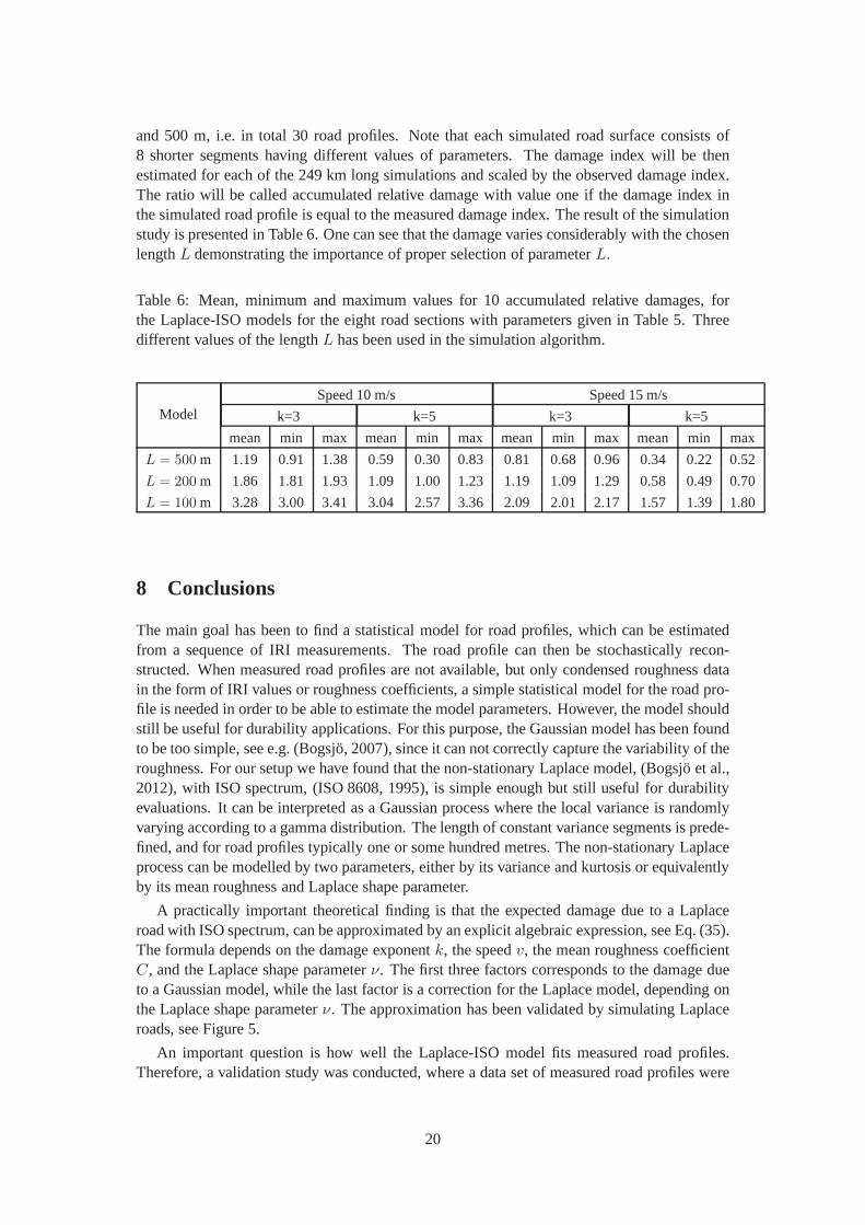
and 500 m, i.e. in total 30 road profiles. Note that each simulated road surface consists of8 shorter segments having different values of parameters. The damage index will be thenestimated for each of the 249 km long simulations and scaled by the observed damage index.The ratio will be called accumulated relative damage with value one if the damage index inthe simulated road profile is equal to the measured damage index. The result of the simulationstudy is presented in Table 6. One can see that the damage varies considerably with the chosenlengthL demonstrating the importance of proper selection of parameterL.

Table 6: Mean, minimum and maximum values for 10 accumulatedrelative damages, forthe Laplace-ISO models for the eight road sections with parameters given in Table 5. Threedifferent values of the lengthL has been used in the simulation algorithm.

ModelSpeed 10 m/s Speed 15 m/s

k=3 k=5 k=3 k=5

mean min max mean min max mean min max mean min max

L = 500 m 1.19 0.91 1.38 0.59 0.30 0.83 0.81 0.68 0.96 0.34 0.22 0.52

L = 200 m 1.86 1.81 1.93 1.09 1.00 1.23 1.19 1.09 1.29 0.58 0.49 0.70

L = 100 m 3.28 3.00 3.41 3.04 2.57 3.36 2.09 2.01 2.17 1.57 1.39 1.80

8 Conclusions

The main goal has been to find a statistical model for road profiles, which can be estimatedfrom a sequence of IRI measurements. The road profile can thenbe stochastically recon-structed. When measured road profiles are not available, butonly condensed roughness datain the form of IRI values or roughness coefficients, a simple statistical model for the road pro-file is needed in order to be able to estimate the model parameters. However, the model shouldstill be useful for durability applications. For this purpose, the Gaussian model has been foundto be too simple, see e.g. (Bogsjö, 2007), since it can not correctly capture the variability of theroughness. For our setup we have found that the non-stationary Laplace model, (Bogsjö et al.,2012), with ISO spectrum, (ISO 8608, 1995), is simple enoughbut still useful for durabilityevaluations. It can be interpreted as a Gaussian process where the local variance is randomlyvarying according to a gamma distribution. The length of constant variance segments is prede-fined, and for road profiles typically one or some hundred metres. The non-stationary Laplaceprocess can be modelled by two parameters, either by its variance and kurtosis or equivalentlyby its mean roughness and Laplace shape parameter.

A practically important theoretical finding is that the expected damage due to a Laplaceroad with ISO spectrum, can be approximated by an explicit algebraic expression, see Eq. (35).The formula depends on the damage exponentk, the speedv, the mean roughness coefficientC, and the Laplace shape parameterν. The first three factors corresponds to the damage dueto a Gaussian model, while the last factor is a correction forthe Laplace model, depending onthe Laplace shape parameterν. The approximation has been validated by simulating Laplaceroads, see Figure 5.

An important question is how well the Laplace-ISO model fits measured road profiles.Therefore, a validation study was conducted, where a data set of measured road profiles were

20

used. The eight road sections represent different types of roads as well as different geographi-cal locations. The conclusions of the study can be summarized as

1. We have demonstrated that the non-stationary Laplace model having observed spectrumreproduces the damage indices very well.

2. We investigated whether the simpler Laplace-ISO model could be used instead. Simplyreplacing the observed spectrum by the an estimated ISO spectrum gave unsatisfactoryaccuracy. However, by estimating the parameters from observed damage values, a “use-ful” Laplace-ISO model was found for the studied roads.

3. We found that the presented approach to estimate Laplace-ISO models from IRI se-quences is useful for reconstruction of road profiles when profile measurements are notavailable.

Some of measured road profiles are not statistically homogeneous and in order to improve afit of Laplace modes to data one could consider to split it in shorter segments in which homo-geneity is more likely, e.g. 5 km long segments. This would result in larger set of estimatedmodels which would allow to study the long term distributionfor the parametersC andν inthe data and then to validate Eq. (39). However, these investigations are outside of the scopeof the present study and will be conducted in the future.

There are several advantages to use the Laplace road profile model with ISO spectrum

• a small number of parameters are needed to define it (the roughness coefficient,C, theLaplace shape parameter,ν, and the length of constant variance road segment,L),

• the parametersC andν can be estimated from the sequence of IRI, see Eq. (26) whichis often available, and

• the expected damage of a response of a vehicle, modelled by a linear filter havingLaplace-ISO road as an input, can be accurately approximated by an explicit formuladepending only on the Laplace parameters,(C, ν), the damage exponent,k, and thespeedv, see e.g. Eq. (35).

The last property is particularly convenient for sensitivity studies since lengthy simulationscan be avoided. It can also be used for estimation of Laplace parameters and for classificationpurposes.

9 Acknowledgments

This work is partially supported by a research project financed by DAF, Daimler, MAN, Scaniaand Volvo. Further, we are thankful to Scania for supplying us with road profile data.

References

P. Andrén. Power spectral density approximations of longitudinal road profiles.Int. J. VehicleDesign, 40:2–14, 2006.

J. S. Bendat. Probability functions for random responses: Prediction of peaks, fatigue damageand catastrophic failures. Technical report, NASA, 1964.

21

A. K. Bengtsson and I. Rychlik. Uncertainty in fatigue life prediction of structures subject toGaussian loads.Probabilistic Engineering Mechanics, 24:224–235, 2009.

K. Bogsjö, K. Podgorski, and I. Rychlik. Models for road surface roughness.Vehicle SystemDynamics, 50:725–747, 2012.

K. Bogsjö. Road Profile Statistics Relevant for Vehicle Fatigue. PhD thesis, MathematicalStatistics, Lund University, 2007.

K. Bogsjö and I. Rychlik. Vehicle fatigue damage caused by road irregularities.Fatigue &Fracture of Engineering Materials & Structures, 32:391–402, 2009.

P. A. Brodtkorb, P. Johannesson, G. Lindgren, I. Rychlik, J.Rydén, and E. Sjö. WAFO –a Matlab toolbox for analysis of random waves and loads. InProceedings of the 10thInternational Offshore and Polar Engineering conference,Seattle, volume III, pages 343–350, 2000.

B. Bruscella, V. Rouillard, and M. Sek. Analysis of road surfaces profiles.ASCE Journal ofTransportation Engineering, 125:55–59, 1999.

D. Charles. Derivation of environment descriptions and test severities from measured roadtransportation data.Journal of the IES, 36:37–42, 1993.

C. J. Dodds and J. D. Robson. The description of road surface roughness.Journal of Soundand Vibration, 31:175–183, 1973.

T. D. Gillespie, M. W. Sayers, and C. A. V. Queiroz. The international road roughness experi-ment: Establishing correlation and calibration standard for measurement. Technical ReportNo. 45, The World Bank, 1986.

A. González, E. J. O’brie, Y.-Y. Li, and K. Cashell. The use ofvehicle acceleration measure-ments to estimate road roughness.Vehicle System Dynamics, 46:483–499, 2008.

J. G. Howe, J. P. Chrstos, R. W. Allen, T. T. Myers, D. Lee, C.-Y. Liang, D. J. Gorsich, andA. A. Reid. Quarter car model stress analysis for terrain/road profile ratings.Int. J. VehicleDesign, 36:248–269, 2004.

ISO 8608. Mechanical vibration - road surface profiles - reporting of measured data, ISO8608:1995(E). International Organization for Standardization, ISO, 1995.

S. Kotz, T. J. Kozubowski, and K. Podgórski.The Laplace Distribution and Generaliza-tions: A Revisit with Applications to Communications, Economics, Engineering and Fi-nance. Birkhaüser, Boston, 2001.

O. Kropác and P. Múcka. Non-standard longitudinal profiles of roads and indicators for theircharacterization.Int. J. Vehicle Design, 36:149–172, 2004.

O. Kropác and P. Múcka. Indicators of longitudinal road unevenness and their mutual rela-tionships.Road Materials and Pavement Design, 8:523–549, 2007.

R. P. La Barre, R. T. Forbes, and S. Andrew. The measurement and analysis of road surfaceroughness. Report 1970/5, Motor Industry Research Association, 1969.

M. A. Miner. Cumulative damage in fatigue.Journal of Applied Mechanics, 12:A159–A164,1945.

22

H. M. Ngwangwa, P. S. Heyns, F. J. J. Labuschagne, and G. K. Kululanga. Reconstruction ofroad defects and road roughness classification using vehicle responses with artificial neuralnetworks simulation.Journal of Terramechanics, 47:97–111, 2010.

A. Palmgren. Die Lebensdauer von Kugellagern.Zeitschrift des Vereins Deutscher Ingenieure,68:339–341, 1924.In German.

V. Rouillard. Using predicted ride quality to characterisepavement roughness.Int. J. VehicleDesign, 36:116–131, 2004.

V. Rouillard. Decomposing pavement surface profiles into a Gaussian sequence.Int. J. VehicleSystems Modelling and Testing, 4:288–305, 2009.

I. Rychlik. A new definition of the rainflow cycle counting method. International Journal ofFatigue, 9:119–121, 1987.

I. Rychlik. On the ‘narrow-band’ approximation for expected fatigue damage.ProbabilisticEngineering Mechanics, 8:1–4, 1993.

M. Shinozuka. Simulation of multivariate and multidimensional random processes.The Jour-nal of the Acoustical Society of America, 49:357–368, 1971.

WAFO Group. WAFO – a Matlab toolbox for analysis of random waves and loads, tutorial forWAFO 2.5. Mathematical Statistics, Lund University, 2011a.

WAFO Group. WAFO – a Matlab Toolbox for Analysis of Random Waves and Loads, Version2.5, 07-Feb-2011. Mathematical Statistics, Lund University, 2011b.Web:http://www.maths.lth.se/matstat/wafo/ (Accessed 12 August 2012).

Appendix

A Sketch of derivation of approximation (30)

We assume that the rainflow damage can be computed for a response observed for each of thesegments with constant variance separately and then added.(This is a reasonable approxima-tion if the mean response is constant for longer period of time.) Under this assumption

E[Dv(k, 1, ν)] = E[Dv(k, 1, 0)]E[Rk/2],

by independence of the factorsRj and Gaussianity of road roughness. Next

E[Rk/2] =

∫ ∞

0

rk/2 fR(r) dr = νk/2Γ(k/2 + 1/ν)

Γ(1/ν).

Finally, for a Gaussian model, one can show that for any pair of nonzero speedsv, v0 one hasthat

E[Dv(k, 1, 0)]/vk/2−1 = E[Dv0(k, 1, 0)]/v

k/2−1

0, (41)

which shows Eq. (30).

23

For simplicity Eq. (41) will be demonstrated only for Shinozuka method, (Shinozuka,1971), to simulate Gaussian processes. Consider the linearresponseYv(x) to Gaussian roadprofile having standard ISO spectrum (roughness coefficientC = 14.4);

Yv(x) =√C

n∑

i=1

Ω−1

i |Hv(Ωi)|√∆Ωcos(Ωi x+ φi). 0 ≤ x ≤ L.

Employing the relationωi = Ωi v and thatHv(Ω) = H(Ω v) then, witht = x/v, the lastequation can be written as follows

Yv(x) =√v√C

n∑

i=1

ω−1

i |H(ωi)|√∆ω cos(ωi t+ φi) =

√vY (t), 0 ≤ t ≤ L/v.

Denote bydk damage growth intensity inY (t) then

E[Dv(k, 1, 0)] =1

L·(

L

vvk/2dk

)

, (42)

and henceE[Dv(k, 1, 0)]/vk/2−1 = dk independently ofv proving the relation (41).

B MATLAB code for model simulation

For readers convenience we present the MATLAB codes used to simulate responses to theGaussian and the non-stationary Laplace models for the roadprofile. From a sequence of IRI,code for estimation of the Gaussian and non-stationary Laplace models is given, as well asdirections for simulating the non-stationary Gaussian model. Finally, code for calculation ofthe expected damage is given.

In the code some functions from the WAFO (Brodtkorb et al., 2000; WAFO Group, 2011a)toolbox are used, which can be downloaded free of charge, (WAFO Group, 2011b). The sta-tistical functionsrndnorm andrndgam are also available in the MATLAB statistics toolboxthroughnormrnd andgamrnd. Note that WAFO also contains functions to find rainflowranges used to estimate fatigue damage.

The length of the simulated function will be 5 km and the sampling interval 5 cm. Thefollowing code can be used to compute the spectrum.

>> dx=0.05; Lp=5000; NN=ceil(Lp/dx)+1; xx=(0:NN-1)’*dx;>> w = pi/dx*linspace(-1,1,NN)’; dw=w(2)-w(1);>> wL=0.011*2*pi; wR=2.83*2*pi;;>> S=zeros(size(w));>> ind=find(abs(w)>=wL & abs(w)<=wR);>> S(ind)=w(ind).^(-2)/28.8;>> G=fftshift(sqrt(S))/sqrt(dx/dw/NN);>> kernel=fftshift(real(ifft(G)));>> figure, plot(w*dx/dw,kernel)

The kernelg(x) is introduced through its Fourier transformG(Ω) = Fg(Ω). We usea normalizedg(x) so that the integral

∫

g(x)2 dx = 1, and hence we need an additionalparameterσ, i.e. the standard deviation of the road, in the code denotedby SD. If the load isGaussian thenσ is constant for whole lengthLp and need to be estimated from the signal.This is not a trivial problem since the true spectrum often differs from the ISO one, but we donot go into details in this issues.

The transfer functionHv(Ω) given by Eq. (10) is computed by

24

>> v=5; ms=3400; ks=270000; cs=6000; mu=350; kt=950000; ct=300;>> wv = w*v; i=sqrt(-1);>> S0=1+ms*wv.^2./(ks-ms*wv.^2+i*cs*wv);>> S1=kt-mu*wv.^2+i*ct*wv-ms*(ks+i*cs*wv).*wv.^2./(-ms*wv.^2+ks+i*cs*wv);>> S2=ms*wv.^2.*(kt+i*ct*wv);>> H=fftshift(S2.*S0./S1);

We turn now to simulation of Gaussian and Laplace models.

B.1 Gaussian model

First a Gaussian white noise processInpG is generated, then the road profile and quartervehicle responsezG andyG, respectively, are computed by means of FFT.

>> InpG=rndnorm(0,1,NN,1); SD=5;>> zG = SD*sqrt(dx)*real(ifft(fft(InpG).*G));>> figure, subplot(2,1,1), plot(xx,zG)>> yG = SD*sqrt(dx)*real(ifft(fft(InpG).*G.*H));>> subplot(2,1,2), plot(xx,yG)

B.2 Non-stationary Laplace model

In the Laplace model it is assumed that parameterσ is constant for a short segment of aroad, here 200 metres. First the shape parameterν, see Eq. (25), is computed from roadprofile kurtosiskurt, here set to 9. This determines the gamma distributed randomvariancesR. Then the modulation processmod is evaluated and finally road elevationzL and quartervehicle responseyL are computed.

>> L=200; M=ceil(L/dx); NM=ceil(NN/M);>> kurt=9; nu=(kurt-3)/3;>> R=nu*rndgam(1/nu,1,1,NM);>> mod=[];>> for j=1:NM;>> mod=[mod; sqrt(R(j))*ones(M,1)];>> end>> zL = SD*sqrt(dx)*real(ifft(fft(InpG.*mod(1:NN)).*G));>> figure, subplot(2,1,1), plot(xx,zL)>> yL = SD*sqrt(dx)*real(ifft(fft(InpG.*mod(1:NN)).*G.*H));>> subplot(2,1,2), plot(xx,yL)

Note that in the code the same sample of a Gaussian white noiseInpG has been used togenerate the Gaussian and non-stationary Laplace models ofthe road profile. This is done tofacilitate visual comparison of the simulated records.

B.3 Estimation of non-stationary Laplace model

Here we assume that from some database the sequence of IRI areavailable sampled also at200 metres. The sequence is saved in a vectorIRI.

>> Ci=(IRI/2.21).^2;>> C=mean(Ci);>> nu=var(Ci)/C^2;>> SD=28.8*C;

25

The estimated parametersC andnu of the non-stationary Laplace model can then be usedfor simulating profiles. Note that if the simulated gamma variablesR are replaced by a corre-sponding vector of observed normalized variancesR=Ci/C, the same simulation code can beused for simulating a non-stationary Gaussian profile.

B.4 Expected damage

Here we check the result of Eq. (30); compare Figure 5. The following code simulates Laplaceroads with different shape parametersν and calculates the observed the fatigue damage index,which is compared with the theoretical formula (30).

>> NN=5*10^5; dx=0.05; L=100; Nsim=20; k=5; v0=10; vv=0:0.2:4;>> nu=0.05:0.05:4; Knu=nu.^(k/2).*gamma(k/2+1./nu)./gamma(1./nu);>> Dv0 = ISOdam(vv,v0,k,dx,NN,L,Nsim);>> d_k=mean(Dv0(1,:));>> figure>> semilogy(vv,mean(Dv0’),’r’)>> hold on>> plot(nu,d_k*Knu,’k’)>> v=25;>> Dv = ISOdam(vv,v,k,dx,NN,L,10);>> plot(vv,mean(Dv’),’g’)>> plot(nu,(v/v0)^(k/2-1)*d_k*Knu,’k’)>> Dv_400 = ISOdam(vv,v,k,dx,NN,400,10);>> plot(vv,mean(Dv_400’),’b--’)

The code needs two functions calledISOdam.m, simulating Laplace roads and calculatingdamage

>> function DDk = ISOdam(vv,v,k,dx,NN,L,Nsim)>> %ISOdam Simulate Laplace roads and calculate damage>> % Call: DDk = ISOdam(vv,v,K,dx,NN,L,Nsim)>> % vv = parameter in Gamma model>> % v = speed>> % k = exponent in damage>> % dx = space sampling step>> % NN = number of simulated points>> % L = length of the constant variance segment>> % Nsim = number of simulated damages>> M=ceil(L/dx); wL=0.011*2*pi; wR=2.83*2*pi; NM=ceil(NN/M);>> Nhh=200; hh=hann(2*Nhh);>> w = pi/dx*linspace(-1,1,NN)’; dw=w(2)-w(1);>> Siso=zeros(size(w));>> ind=find(abs(w)>=wL & abs(w)<=wR); Siso(ind)=w(ind).^(-2);>> Siso=Siso/trapz(w,Siso);>> G=fftshift(sqrt(Siso))/sqrt(dx/dw/NN);>> H=fftshift(FilterH(w,v));>> DDk=zeros(length(vv),Nsim);>> for i1=1:length(vv)>> vv4=vv(i1);>> Dk=zeros(1,Nsim);>> for i2=1:Nsim>> InpG=rndnorm(0,1,NN,1);>> R=ones(NM,1);>> if vv4>0.025

26

>> R=vv4*rndgam(1/vv4,1,1,NM);>> end>> ONES=ones(M,1);>> mod=[];>> for j=1:NM;>> mod=[mod; sqrt(R(j)).*ONES];>> end>> xL = sqrt(dx)*real(ifft(fft(InpG.*mod(1:NN)).*G));>> xL(1:Nhh)=xL(1:Nhh).*hh(1:Nhh);>> xL(end-Nhh+1:end)=xL(end-Nhh+1:end).*hh(Nhh+1:end);>> FInpL = fft(xL).*H;>> LsimISO4 = real(ifft(FInpL));>> respISO4=[(0:NN-1)’*dx LsimISO4];>> tpISO4=dat2tp(respISO4); rfcISO4=tp2rfc(tpISO4);>> Dam5rfcISO4=sum((rfcISO4(:,2)-rfcISO4(:,1)).^k);>> Dk(i2)=Dam5rfcISO4;>> end>> DDk(i1,:)=Dk/NN/dx;>> end>> end

andFilterH.m defining the transfer function.

>> function H0 = FilterH(w,v)>> %FilterH Calculates transfer function of force response filter>> % Call: H0 = FilterH(w,v)>> % w = spacial angular frequency>> % v = speed>> ms=3400; ks=270000;cs=6000; mu=350; kt=950000; ct=300;>> wv = w*v; i=sqrt(-1);>> S0=1+ms*wv.^2./(ks-ms*wv.^2+i*cs*wv);>> S1=kt-mu*wv.^2+i*ct*wv-ms*(ks+i*cs*wv).*wv.^2./(-ms*wv.^2+ks+i*cs*wv);>> S2=ms*wv.^2.*(kt+i*ct*wv);>> H0=S2.*S0./S1;>> end

27