Preliminary Design Methods - University Of Marylandspacecraft.ssl.umd.edu/academics/483F06/483L20... · Feb 19 2003 ENAE 691 R.Farley NASA/GSFC Satellite Design Course Spacecraft

Feb 19 2003 ENAE 691 R.Farley NASA/GSFC

Satellite Design Course Spacecraft Configuration

Structural DesignPreliminary Design Methods

This material was developed by Rodger Farley (NASA GSFC) for

ENAE 691 (Satellite Design)

Feb 19 2003 ENAE 691 R.Farley NASA/GSFC2

Source of Launch Vehicle Loads


Typical Loads Time-Line ProfileMax Q

MECOSECO

H2 vehicle to geo-transfer orbit

3rd stage2nd stage

1st stage


Design Requirements, LoadsMaterial processing, assembling, handlingTestingTransportationLaunch handlingLaunch loads

• Steady state accelerations (max Q, end of burn stages)

• Sinusoidal vibrations, transient (lift off, transonic, MECO, SECO) and steady (resonant burn from solid rocket boosters)

• Acoustic and mechanical random accelerations (lift off, max Q)

• Shock vibrations (payload separation from upper stage adapter)

• Depressurization

Orbit Loads spin-up, de-spin, thermal, deployments, maneuvers


Configuration Types LEO stellar pointing

Low inclination XTE, HSTHigh inclination WIRE

Articulated solar array Fixed solar array sun-sync orbit


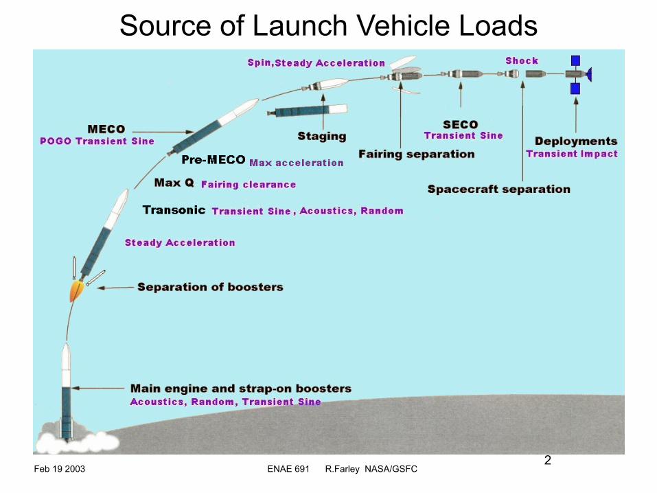
Configuration Types GEO nadir pointing

Articulated s/a spin once per 24 hoursTDRSS A

Intelsat V


Configuration Types HEO

AXAF-1 CHANDRA required to stare uninterrupted

250m long wire booms, ¼ rpm

IMAGE 2000


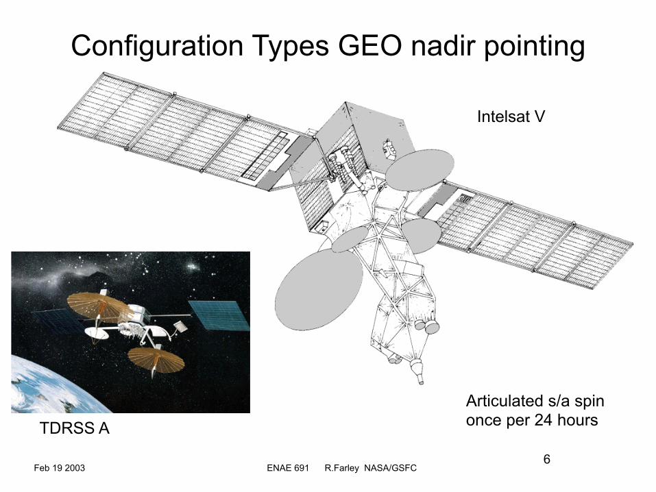
Configuration types misc

MAP at L2Magellan to Venus

Lunar Prospector

Body-mounted s/a

High-gain antenna

Cylindrical, body-mounted solar array

Sun shield


Structural Configuration Examples• Cylinders and Cones high buckling resistance

• Box structures hanging electronics and equipment

• Triangle structures sometimes needed

• Rings transition structures and interfaces

• Trusses extending a ‘hard point’ (picking up point loads)

• As much as possible, payload connections should be kinematic• Skin Frame, Honeycomb Panels, Machined Panels, Extrusions

NOTE: ALWAYS PROVIDE A STIFF AND DIRECT LOAD PATH! AVOID BENDING!

STRUCTURAL JOINTS ARE BEST IN SHEAR!


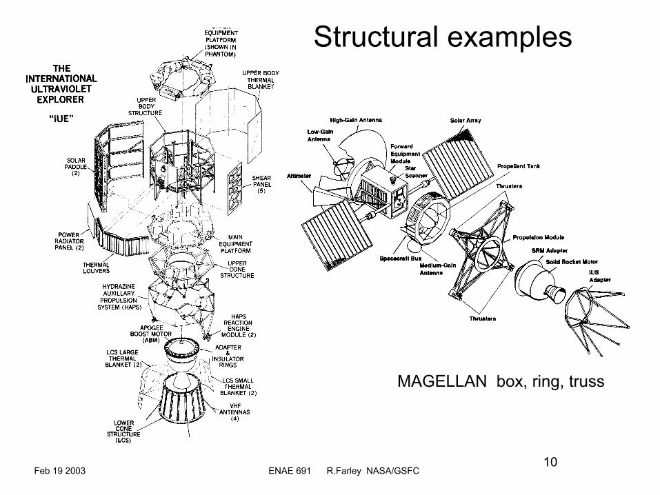
Structural examples

MAGELLAN box, ring, truss


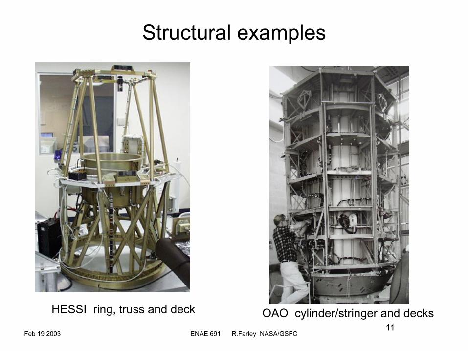
Structural examples

OAO cylinder/stringer and decksHESSI ring, truss and deck


Structural examples

Reaction wheel ‘pyramid’

Rain Radar

TRMM

Bus structure, cylinder, machined and honeycomb panels

Instrument support truss and panel structure


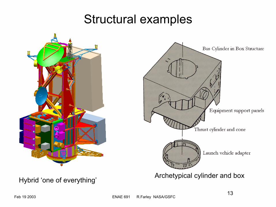
Structural examples

Archetypical cylinder and box Hybrid ‘one of everything’


Structural examplesEOS aqua, bus

Hard points created at intersections

“Egg crate” composite panel bus structure


Structural examples

COBE

Delta II version

COBE

STS version

5000 kg !

2171 kg !


Modular AssemblyInstrument Module –optics, detectorBus Module (house keeping)Propulsion Module

Modules allow separate organizations, procurements, building and testing schedules. It all comes together at observatory integration and test (I&T)

Interface control between modules is very important: structural, electrical, thermal

AXAF


Anatomy of s/c

Instrument module

Bus module

Propulsion module

Launch Vehicle adapter

Interface structure

Axial viewing, telescope type

Solid kick motor, equatorial mount

Station-keeping hydrazine, polar mountReaction wheels

Deck-mounted or wall-mounted boxes

Kinematic Flexure mounts to remove enforced displacement loads


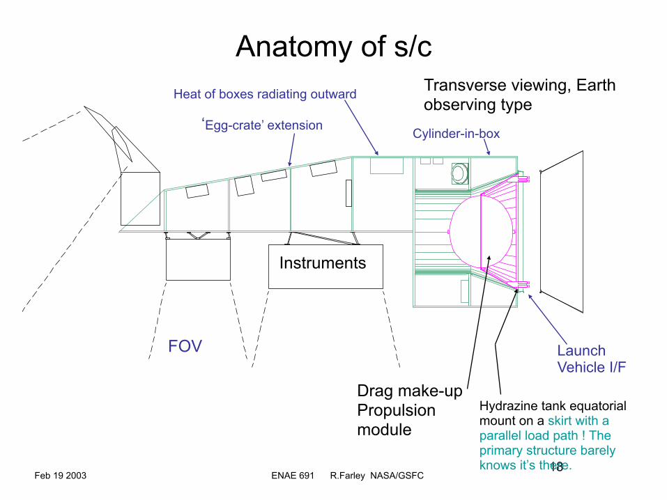
Anatomy of s/cTransverse viewing, Earth observing type

Launch Vehicle I/F

Drag make-up Propulsion module

FOV

Instruments

Cylinder-in-box‘Egg-crate’ extension

Heat of boxes radiating outward

Hydrazine tank equatorial mount on a skirt with a parallel load path ! The primary structure barely knows it’s there.


Attaching distortion-sensitive components

Ball-in-cone, Ball-in-vee, Ball on flat

Breathes from point ‘3’

2,2,2

Bi-pod legs, tangential flexures

Breathes from center point

Rod flexures arranged in 3,2,1

Breathes from point ‘3’

1,1,1,1,1,1 3

2

1

1

2

3Note: vee points towards cone

3,2,1


General Arrangement Drawings

• Stowed configuration in Launch Vehicle• Transition orbit configuration• Final on-station deployed configuration• Include Field of View (FOV) for instruments and thermal

radiators, and communication antennas, and attitude control sensors


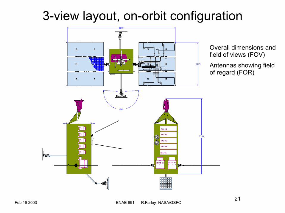
3-view layout, on-orbit configuration

Overall dimensions and field of views (FOV)

Antennas showing field of regard (FOR)


3-view layout, launch configuration

Make note of protrusions into payload envelope

Omni antennasHigh gain antenna, stowed

Star trackers PAF

Solar array panels array drive

Torquer bars


Spacecraft Drawing in Launch Vehicle

XTE in Delta II 10’ fairingFairing access port for the batteries

Pre-launch electrical access “red-tag” item

Launch Vehicle electrical interface


Drawing of deployment phase

EOS aqua

Pantograph deployment mechanism


Launch Vehicle Interfaces and VolumesPayload Fairings


Payload Envelope

If frequency requirements are not met, or for protrusions outside the designated envelope, Coupled Loads Analysis (CLA) are required to qualify the design, in cooperation with the LV engineers.

For many vehicles, if the spacecraft meets minimum lateral frequency requirements, then the envelope accounts for payload and fairing dynamic motions.


Launch Vehicle Payload Adapters

6019 3-point adapter 6915 4-point adapter

“V-band” clamp, or “Marmon” clamp-band

Clamp-band

Shear Lip


Structural MaterialsMaterial ρ

(kg/m3)E (GPa)

Fty(MPa)

E/ρ Fty/ρ α(µm/m K˚)

κ(W/m K˚)

Aluminum6061-T67075-T651

28002700

6871

276503

2426

98.6186.3

23.623.4

167130

MagnesiumAZ31B 1700 45 220 26 129.4 26 79

Titanium6Al-4V 4400 110 825 25 187.5 9 7.5

BerylliumS 65 AS R 200E

2000-

304-

207345

151-

103.5-

11.5-

170

FerrousINVAR 36AM 350304L annealed

4130 steel

8082770078007833

150200193200

62010341701123

18.5262525

76.7134.321.8143

1.6611.917.212.5

1440-601648

Heat resistantNon-magneticA286Inconel 600Inconel 718

794484148220

200206203

5852061034

252425

73.624.5125.7

16.4-23.0

12-12

Metallic Guide


Materials Guide Definitionsρ mass density

E Young’s modulus

Fty material allowable yield strength Note: Pa = Pascal = N/m2

E / ρ specific stiffness, the ratio of stiffness to density

Fty / ρ specific strength, the ratio of strength to density

α coefficient of thermal expansion CTE

κ coefficient of thermal conductivity

Material Usage Conclusions: USE ALUMINUM WHEN YOU CAN!!!Aluminum 7075 and Titanium 6Al-4V have the greatest strength to mass ratio

Beryllium has the greatest stiffness to mass ratio and high damping

4130 Steel has the greatest yield strength

INVAR has the lowest coefficient of thermal expansion, but difficult to process

Titanium has the lowest thermal conductivity, good for metallic isolators

(expensive, toxic to machine, brittle)


Metallic Materials Usage Guide

High strength to weight, good machining, low cost and available

High strength to weight, low CTE, low thermal conductivity, good at high temperatures

High stiffness, strength, low cost, weldable

High stiffness, strength at high temperatures, oxidation resistance and non-magnetic

Very high stiffness to weight, low CTE

Aluminum

Titanium

Steel

Heat-resistant Steel

Beryllium

Poor galling resistance, high CTE

Expensive, difficult to machine

Heavy, magnetic, oxidizes if not stainless steel. Stainless galls easily

Heavy, difficult to machine

Expensive, brittle, toxic to machine

Truss structure, skins, stringers, brackets, face sheets

Attach fittings for composites, thermal isolators, flexures

Fasteners, threaded parts, bearings and gears

Fasteners, high temperature parts

Mirrors, stiffness critical parts

Advantages Disadvantages Applications


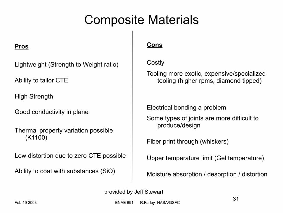
Composite Materials

Pros

Lightweight (Strength to Weight ratio)

Ability to tailor CTE

High Strength

Good conductivity in plane

Thermal property variation possible (K1100)

Low distortion due to zero CTE possible

Ability to coat with substances (SiO)

Cons

Costly

Tooling more exotic, expensive/specialized tooling (higher rpms, diamond tipped)

Electrical bonding a problem

Some types of joints are more difficult to produce/design

Fiber print through (whiskers)

Upper temperature limit (Gel temperature)

Moisture absorption / desorption / distortion

provided by Jeff Stewart


Composite Material PropertiesGraphite Fiber Reinforced Plastic (GFRP) density ~ 1800 kg/m3

If aluminum foil layers are added to create a quasi-isotropic zero coefficient of thermal expansion (CTE < 0.1 x10-6 per Co) then density ~ 2225 kg/m3

Aluminum foil layers are used to reduce mechanical shrinkage due to de-sorption / outgassing of water from the fibers and matrix (adhesive,ie. epoxy)

NOTE! A single pin hole in the aluminum foil will allow water de-sorption and shrinkage. This strategy is not one to trust…

Cynate esters are less hydroscopic than epoxies

Shrinkage of a graphite-epoxy optical metering structure due to de-sorption may be described as an asymptotic exponential (HST data):

Shrinkage ~ 27 (1 – e - 0.00113D) microns per meter of length, where D is the number of days in orbit.


Subsystem Mass Estimation TechniquesPreliminary Design Estimates for Instrument Mass

Approximate instrument mass densities, kg / m3

Spectrometers ~ 250

Mass spectrometers ~ 800

Synthetic aperture radar ~ 32

Rain radars ~ 150 thickness / diameter ~ 0.2

Cameras ~ 500

Small instruments ~ 1000

Scaling Laws: If a smaller instrument exists as a model, then if SF is the linear dimension scale factor…

Area proportional to SF2 Mass proportional to SF3

Area inertia proportional to SF4 Mass inertia proportional to SF5

BEWARE THE SQUARE-CUBE LAW! STRESS WILL INCREASE WITH SF!

Frequency proportional to 1/ SF Stress proportional to SF


Typical List of Boxes, Bus ComponentsACS

Reaction wheels Torquer bars Nutation damper Star trackers Inertial reference unit Earth scanner Digital sun sensor Coarse sun sensor Magnetometer ACE electrical box

Communication

S-band omni antenna S-band transponder X-band omni antenna X-band transmitter Parabolic dish reflector 2-axis gimbal Gimbal electronics Diplexers, RF switches Band reject filters Coaxial cable

Power

Batteries Solar array panels Articulation mechanisms Articulation electronics Array diode box Shunt dissipaters Power Supply Elec. Battery a/c ducting

Mechanical

Primary structure Deployment mechanisms Fittings, brackets, struts, equipment decks, cowling, hardware Payload Adapter Fitting

Propulsion

Propulsion tanks Pressurant tanks Thrusters Pressure sensors Filters Fill / drain valve Isolator valves Tubing

Thermal

Radiators Louvers Heat pipes Blankets Heaters Heat straps Sun shield Cryogenic pumps Cryostats

Electrical

C&DH box Wire harness

Instrument electronics

Instrument harness


Mass Estimation, mass fractionsSome Typical Mass Fractions for Preliminary Design

Payload Structure Power Electricalharness

ACS Thermal C&DH Comm Propulsion, dry

LEOnadir(GPM)

37 % 24 % 13 %Fixedarrays

7 % 6 % 4 % 1 % 3 % 5 %26 % w/fuel

LEOstellar(COBE)

52 % 14 % 12 %spins at 1 rpm

8 % 8 % 2 % 3 % 1 % 0 %

GEOnadir(DSP 15)

37 % 22 % 20 %spins at6 rpm

7 % 6 % 0.5 % 2 % 2 % 2 %

Mass fractions as percentage of total spacecraft observatory mass, less fuel

COBE with 52% payload fraction is unusually high and not representative

ACS is Attitude Control System, C&DH is Command and Data Handling, Comm is Communication subsystem


Mass Estimation, RefinementsThe largest contributors to mass are (neglecting the instrument payload)

Structural subsystem (primary, secondary)

Propulsion fuel mass, if required

Power subsystem

The following slides will show the ‘cheat-sheet’ for making preliminary estimates on some of these subsystems

Remember to target a mass margin of ~20% when compared to the throw weight of the launch vehicle and payload adapter capability. There must be room for growth, because evolving from the cartoon to the hardware, it always grows!


Mass Estimation with Mass RatiosMpayload/MDry ~ 0.4 for a first guess

MDry = Mpayload / (Mpayload/MDry) first cut estimate on total dry mass

Calculate total orbital average power required Poa as function of bus mass and payload requirements

Calculate MPower, and solar array area leading to a calculation on drag area

Calculate MFuel, and MPropDry with original MDry and drag area as guide

New Estimate of total dry mass:

MDry = Mpayload + MPower + MPropDry

+ MDry (MStruc/MDry + MElec/MDry + MCDH/MDry + MACS/MDry + MComm/MDry)

Iterate several times to achieve Total Dry Mass

Taking typical values: MDry = Mpayload + MPower + MPropDry +0.45MDry

MWet = MDry + MFuel Total wet mass, observatory launch mass


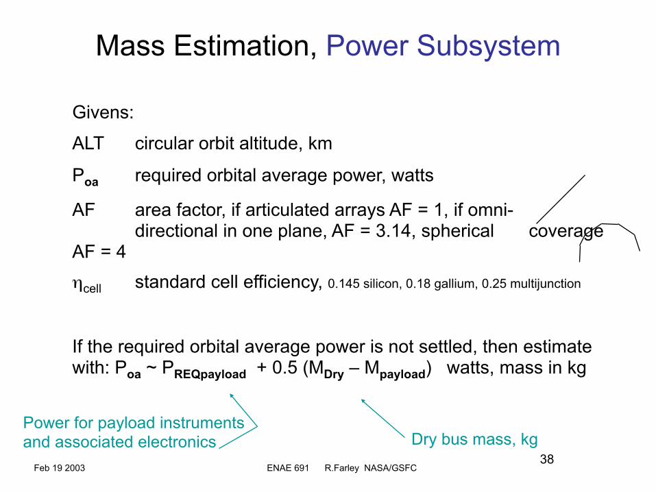
Mass Estimation, Power Subsystem

Givens:

ALT circular orbit altitude, km

Poa required orbital average power, watts

AF area factor, if articulated arrays AF = 1, if omni- directional in one plane, AF = 3.14, spherical coverage AF = 4ηcell standard cell efficiency, 0.145 silicon, 0.18 gallium, 0.25 multijunction

If the required orbital average power is not settled, then estimate with: Poa ~ PREQpayload + 0.5 (MDry – Mpayload) watts, mass in kg

Dry bus mass, kgPower for payload instruments and associated electronics



Total solar array panel area considering energy balance going thru eclipse and geometric area factors, m2

Maximum eclipse-to-daylight time ratio, estimate good for 300<ALT<1000

Required solar array projected area normal to sun, m2

Physical panel area, m2


Mass Estimation, Power SubsystemMass of cells, insulation, wires, terminal boards:

Melec ~ 3.8 x ASA for multi-junction cells kg

Melec ~ 3.4 x ASA for silicon cells kg

Mass of honeycomb substrates:

Msubstrates ~ 2.5 x ASA for aluminum panels kg

Msubstrates ~ 2.0 x ASA for composite panels kg

Mass of solar array panels, electrical and structure:

MPANELS = Melec + Msubstrates kg

Since multi junction cells usually go on composite substrates, and silicon cells went on aluminum substrates, it all comes out in the wash:

MPANELS ~ 5.85 x ASA kg

93% packing efficiency



Mbattery = 0.06 Poa Battery mass, kg Ni-Cads

MPSE = 0.04 Poa Power systems electronics, kg

MSAD = 0.33 Mpanels Solar array drives and electronics, kg

MSAdeploy = 0.27 Mpanels Solar array retention and deployment mechanisms, kg

MPower = Mpanels + MSAD + MSAdeploy + Mbattery + MPSE

Total power subsystem mass estimate, kg

(this can vary greatly due to the peak power input and charging profile allowed. ‘High noon’ power input can be enormous sometimes, depending on orbit inclination and drag reduction techniques)

Tracking array


Mass Estimation, Propulsion Subsystem

Givens:

Isp fuel specific thrust, seconds (227 for hydrazine, 307 bi-prop)ΔV deltaV required for maneuvers during the mission, m/s

TM mission time in orbit, years

YSM years since last solar maximum, 0 to 11 years

AP projected area in the velocity direction, orbital average, m2

ALT circular orbit flight altitude, km

Mdry total spacecraft observatory mass, dry of fuel, kg

Solar array orbital average projected drag area for a tracking solar array that feathers during eclipse


Mass Estimation, Propulsion Subsystem

If the mission requires altitude control, this is the approximate fuel mass for drag over the mission life

Note: g = 9.81 m/s2

Densitymax = 4.18 x 10-9 x e(-0.0136 ALT)

DF = 1 – 0.9 sin [π x YSM / 11]

Densityatm = DF x Densitymax

Approximate maximum atmospheric density at the altitude ALT (km), kg / m3

good for 300 < ALT < 700 km

Density factor, influenced by the 11 year solar maximum cycle (sin() argument in radians)

Corrected atmospheric density, kg / m3

Circular orbit velocity, m/s

Drag force, Newtons

Fuel mass for drag make-up, kg


Mass Estimation, Propulsion SubsystemFuel mass for maneuvering

If maneuvers are conducted at the beginning of the mission (attaining proper orbit):

If the fuel is to be saved for a de-orbit maneuver:

Or expressed as a ratio:


Mass Estimation, Propulsion SubsystemApproximate ΔV to de-orbit to a 50km perigee:

From 400km circular ~ 100 m/s




Remember, the dry mass estimate now includes the mass of the dry prop system components.

This means iterating with a better dry mass estimate for a better fuel calculation.

If the thrusters are too small for one large ΔV de-orbit maneuver, then 2-3 times the calculated fuel maybe required (TRMM experience)

Add 10% for ‘ullage’


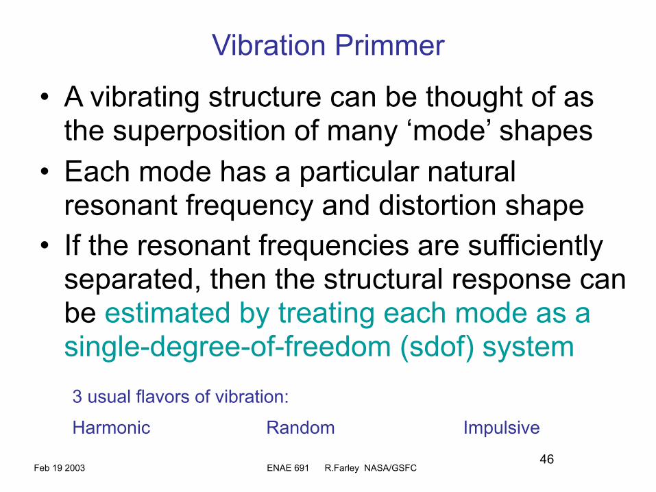
Vibration Primmer

• A vibrating structure can be thought of as the superposition of many ‘mode’ shapes

• Each mode has a particular natural resonant frequency and distortion shape

• If the resonant frequencies are sufficiently separated, then the structural response can be estimated by treating each mode as a single-degree-of-freedom (sdof) system3 usual flavors of vibration:

Harmonic Random Impulsive


Harmonic (sinusoidal) Vibration, sdof

Hz

0.05 typical

Natural frequency of vibration

Recall:

2 π f = ω ‘Circular frequency’, radians / s


Harmonic Vibration, sdof con’t

Typical structural values for Q: 10 to 20

For small amplitude (jitter), or cryo temperatures: Q >100

Resonant Load Acceleration = input acceleration x Q

f is the applied input sinusoidal frequency, Hz

fn is the natural resonant frequency

Harmonic output acceleration = Harmonic input acceleration x T


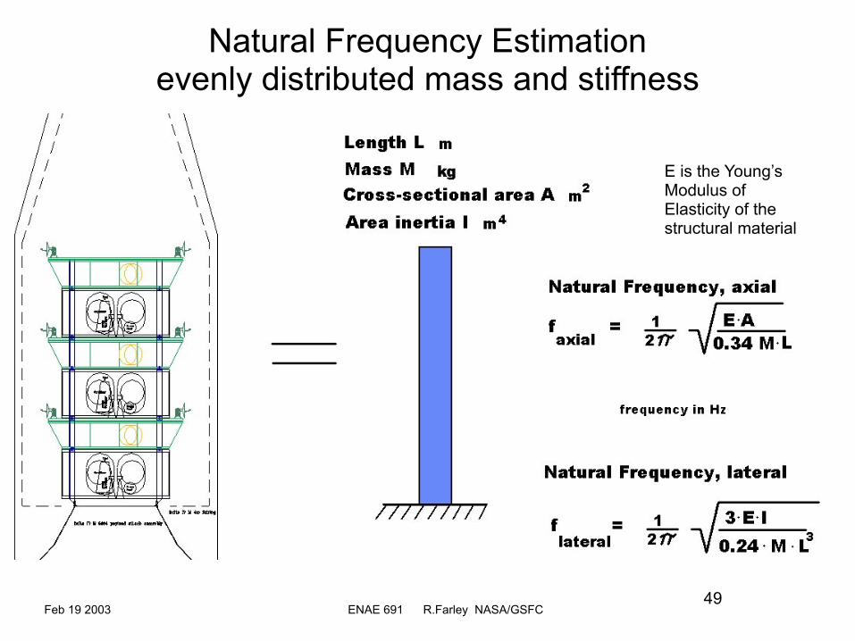
Natural Frequency Estimationevenly distributed mass and stiffness

E is the Young’s Modulus of Elasticity of the structural material


Natural Frequency Estimationdiscrete and distributed mass and stiffness



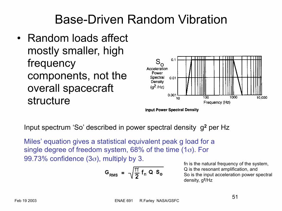
Base-Driven Random Vibration• Random loads affect

mostly smaller, high frequency components, not the overall spacecraft structure

Input spectrum ‘So’ described in power spectral density g2 per Hz

Miles’ equation gives a statistical equivalent peak g load for a single degree of freedom system, 68% of the time (1σ). For 99.73% confidence (3σ), multiply by 3.

fn is the natural frequency of the system, Q is the resonant amplification, and So is the input acceleration power spectral density, g2/Hz

So


Deployable Boom, equations for impact torque

Maximum Impact torque at lock-in, N-m

Hinge point “o”

Io Rotational mass inertia about point “o”, kg-m2

Dynamic system is critically damped

dθ/dt can just be the velocity at time of impact if not critically damped


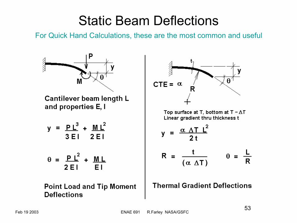
Static Beam DeflectionsFor Quick Hand Calculations, these are the most common and useful


Developing Limit Loads for Structural Design

• Quasi-Static loads– Linear and rotational accelerations + dynamicDynamic Loads included in Quasi-Static:– Harmonic vibration (sinusoidal)– Random vibration (mostly of acoustic origin)– Vibro-acoustic for light panels

• Shock loads• Thermal loads• Jitter

Don’t forget, there are payload mass vs. c.g. height limitations for the launch vehicle’s payload adapter fitting


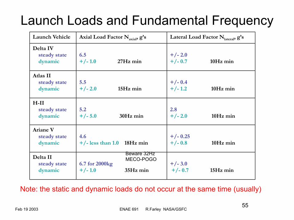
Launch Loads and Fundamental FrequencyLaunch Vehicle Axial Load Factor Naxial, g’s Lateral Load Factor Nlateral, g’s

Delta IV steady state dynamic

6.5+/- 1.0 27Hz min

+/- 2.0+/- 0.7 10Hz min

Atlas II steady state dynamic

5.5+/- 2.0 15Hz min

+/- 0.4+/- 1.2 10Hz min

H-II steady state dynamic

5.2+/- 5.0 30Hz min

2.8+/- 2.0 10Hz min

Ariane V steady state dynamic

4.6+/- less than 1.0 18Hz min

+/- 0.25+/- 0.8 10Hz min

Delta II steady state dynamic

6.7 for 2000kg+/- 1.0 35Hz min

+/- 3.0 +/- 0.7 15Hz min

Note: the static and dynamic loads do not occur at the same time (usually)

Beware 32Hz MECO-POGO


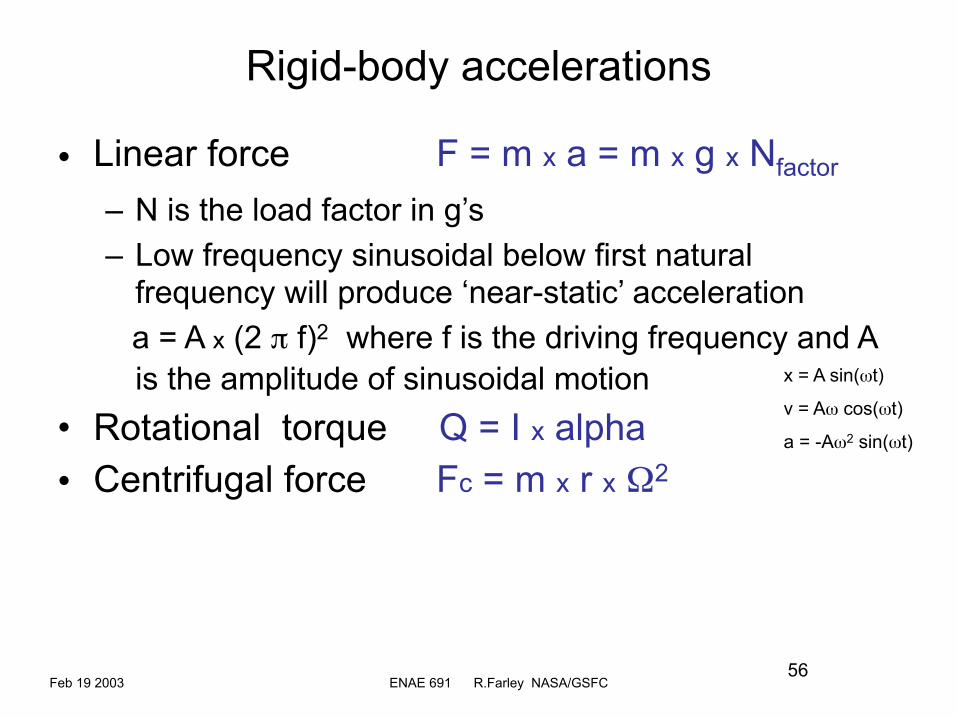
Rigid-body accelerations

• Linear force F = m x a = m x g x Nfactor

– N is the load factor in g’s– Low frequency sinusoidal below first natural

frequency will produce ‘near-static’ acceleration a = A x (2 π f)2 where f is the driving frequency and A

is the amplitude of sinusoidal motion• Rotational torque Q = I x alpha• Centrifugal force Fc = m x r x Ω2

x = A sin(ωt)

v = Aω cos(ωt)

a = -Aω2 sin(ωt)


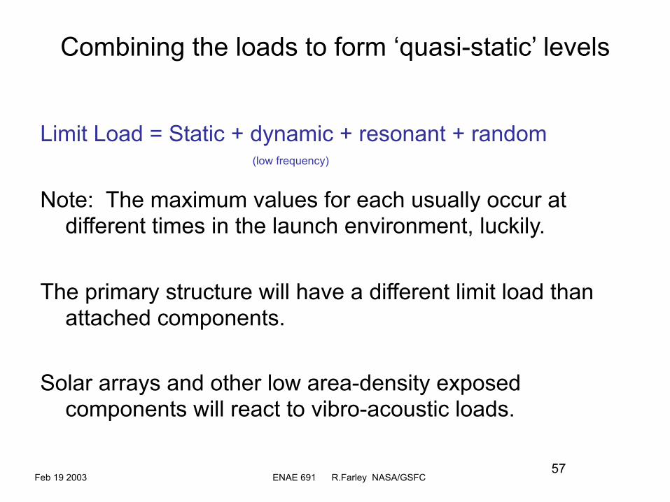
Combining the loads to form ‘quasi-static’ levels

Limit Load = Static + dynamic + resonant + random

Note: The maximum values for each usually occur at different times in the launch environment, luckily.

The primary structure will have a different limit load than attached components.

Solar arrays and other low area-density exposed components will react to vibro-acoustic loads.

(low frequency)


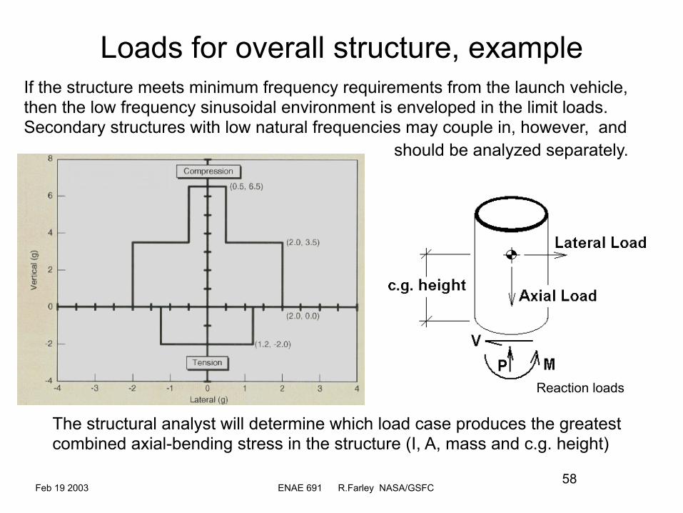
Loads for overall structure, exampleIf the structure meets minimum frequency requirements from the launch vehicle, then the low frequency sinusoidal environment is enveloped in the limit loads. Secondary structures with low natural frequencies may couple in, however, and

The structural analyst will determine which load case produces the greatest combined axial-bending stress in the structure (I, A, mass and c.g. height)

Reaction loads

should be analyzed separately.


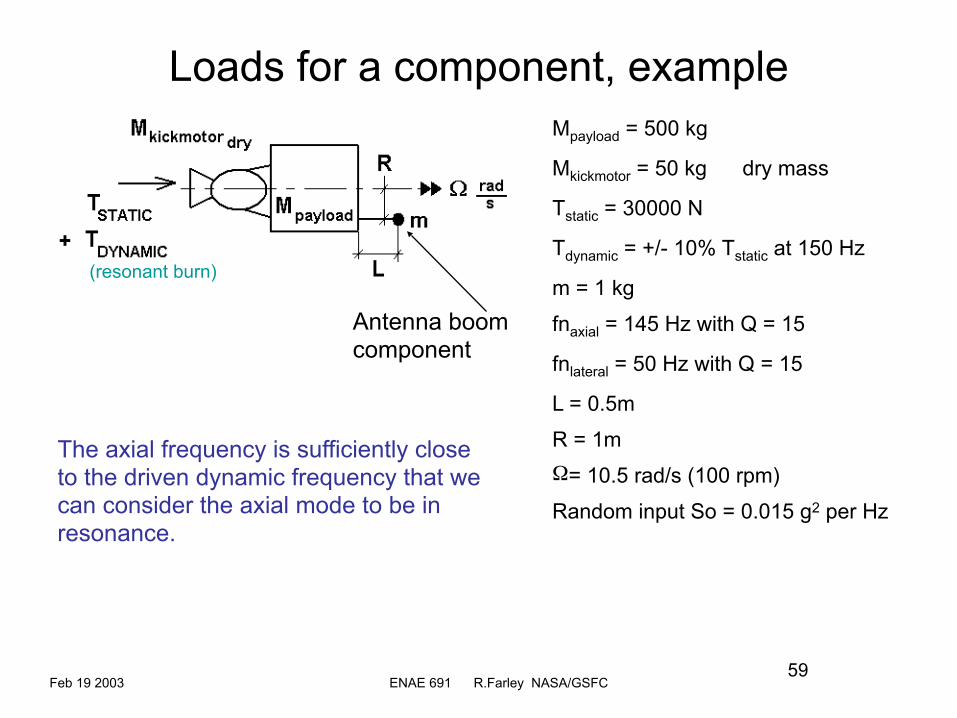
Loads for a component, exampleMpayload = 500 kg

Mkickmotor = 50 kg dry mass

Tstatic = 30000 N

Tdynamic = +/- 10% Tstatic at 150 Hz

m = 1 kg

fnaxial = 145 Hz with Q = 15

fnlateral = 50 Hz with Q = 15

L = 0.5m

R = 1mΩ= 10.5 rad/s (100 rpm)

Random input So = 0.015 g2 per Hz

Antenna boom component

The axial frequency is sufficiently close to the driven dynamic frequency that we can consider the axial mode to be in resonance.

(resonant burn)


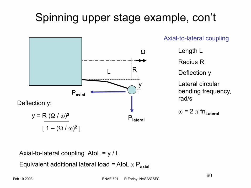
Spinning upper stage example, con’t

y

Axial-to-lateral coupling

Ω

ω = 2 π fnLateral

L R

Length L

Radius R

Deflection y

Lateral circular bending frequency, rad/s

y = R (Ω / ω)2

[ 1 – (Ω / ω)2 ]

Deflection y:

Paxial

Plateral

Axial-to-lateral coupling AtoL = y / L

Equivalent additional lateral load = AtoL x Paxial


Loads for a component, con’t

Static axial acceleration GstaticA = Tstatic / g (Mpayload + Mkickmotor) g’sDynamic axial acceleration GdynA = Tdynamic x Q / g (Mpayload + Mkickmotor) g’sRandom axial acceleration GrmdA = 3 sqr[0.5π fnaxial Q So] g’s

Axial Limit Load Factor, g’s, Naxial = GstaticA + GdynA + GrmdA g’sAxial Limit Load, Newtons, Paxial = g x m x NaxialL

Static lateral acceleration GstaticL = R Ω2 / g + AtoL x Naxial g’sRandom lateral acceleration GrmdL = AtoL x 3 sqr[0.5π fnlateral Q So] g’s

Lateral Limit Load Factor, g’s, Nlateral = GstaticL + GdynL + GrmdL g’sLateral Limit Load, Newtons Plateral = g x m x NlateralMoment at boom base M = L x Plateral


Component Loads, Mass-Acceleration Curve

Applicable Launch Vehicles:

STS

Titan

Atlas

Delta

Ariane

H2

Proton

Scout

Simplified design curve for components on ‘appendage-like’ structures under 80 Hz fundamental frequency


Sizing the Primary Structure rigidity, strength and stability

Factors of safety NASA / INDUSTRY, metallic structures

Factors of safety Verification by Test Verification by Analysis

FS yield 1.25 / 1.10 2.0 / 1.6

FS ultimate 1.4 / 1.25 2.6 / 2.0

Factors of safety for buckling (stability) elements ~ FS buckling = 1.4

(stability very dependent on boundary conditions….so watch out!)


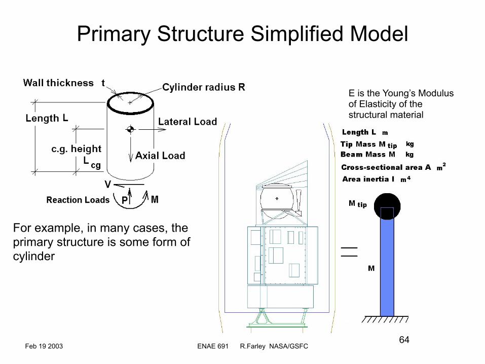
Primary Structure Simplified Model

For example, in many cases, the primary structure is some form of cylinder



Sizing for rigidity (frequency)

Working the equations backwards….

When given frequency requirements from the launch vehicle users guide for 1st major axial frequency and 1st major lateral frequency, faxial, flateral:

Material modulus E times cross sectional area A

Material modulus E times bending inertia I

For a thin-walled cylinder:

I = π R3 t , or t = I / (π R3)

A = 2π R t or t = A / (2π R) Determine the driving requirement resulting in the thickest wall t. Recalculate A and I with the chosen t.

Select material for E, usually aluminum

e.g.: 7075-T6 E = 71 x 109 N/m2

Calculate for a 10% – 15% frequency marginTapering thickness will drop frequency 5% to 12%, but greatly reduce structural mass


Sizing for Strength

Plateraldes = (M + Mtip) g NlimitL Lateral Design Load

Paxialdes = (M + Mtip) g NlimitA Axial Design Load

Design Loads using limit loads and factors of safety

Recalling from mechanics of materials:

axial stress = P/A, bending stress = Mc/I (in a cylinder, the max shear and max compressive stress occur in different areas and so for preliminary design shear is not considered)

Max stress σmax = Paxialdes / A + (Plateraldes Lcg R) / I

Margin of safety MS = {σallowable / (FS x σmax)} – 1 0 < MS acceptable

For 7075-T6 aluminum, the yield allowable , σallowable = 503 x 106 N/m2

With less stress the higher up, the more tapered the structure can be, saving mass


Sizing for Structural StabilityDetermine the critical buckling stress for the cylinder

In the general case of a cone:

Allowable Critical Buckling Stress

Compare critical stress to the maximum stress as calculated in the previous slide. Update the max stress if a new thickness is required.

Margin of safety MS = {σCR /(FSbuckling x σmax)} – 1 0 < MS acceptable

Check top and bottom of cone: σmax, I, moment arm will be different Sheet and stringer construction will save ~ 25% mass


Structural Subsystem MassFor all 3 cases of stiffness, strength, and stability, optimization calls for ‘tapering’ of the structure.

The frequency may drop between 5% to 12% with tapering

But the primary structural mass savings may be 25% to 35% - a good trade

Secondary structure (brackets, truss points, interfaces….) may equal or exceed the primary structure. An efficient structure, assume secondary structure = 1.0 x primary structure. A typical structure, assume 1.5.

So, if the mass calculated for the un-optimized constant-wall thickness cylinder (primary structure) is MCYL, then the typical structure (primary + secondary):

MSTRUCTURE ~ (2.0 to 3.5) x MCYL

This number can vary significantly

Documents

Preliminary Design Methods - University Of Marylandspacecraft.ssl.umd.edu/academics/483F06/483L20... · Feb 19 2003 ENAE 691 R.Farley NASA/GSFC Satellite Design Course Spacecraft