Embed Size (px)
Citation preview

PREFEASIBILITY STUDIES FOR MINI HYDRO POWER GENERATION ON
KINTAMPO FALLS
By
Charles Ken Adu Boahen
A thesis submitted to the Graduate School,
Kwame Nkrumah University of Science and Technology
In partial fulfillment of the requirement for the degree of
Master of Science Renewable Energy Technologies
Department of Mechanical Engineering
College of Engineering
June 2013

ii
DECLARATION
I hereby declare that this submission is my own work towards the MSc and that, to the
best of my knowledge, it contains no material previously published by another person nor
material which has been accepted for the award of any other degree of the University,
except where due acknowledgement has been made in the text.
CHARLES KEN ADU BOAHEN ……………………..…… ……. ……………..
(Student - PG6307511) (Signature) (Date)
Certified by:
DR. GABRIEL TAKYI ………………….....………………
……………………..
(Supervisor) (Signature) (Date)
Certified by:
DR. S.M SACKEY ………………….....………………
………………………
(Head of Dept.) (Signature) (Date)

iii
ACKNOWLEDGEMENT
To Jehovah God be the glory for the great things he has done and helping me to
accomplish this task. My special thanks go to my supervisor Dr. Gabriel Takyi for the
guidance, time and support he gave me throughout this study. I wish to acknowledge the
help from Messer‟s Daniel Duah and Obed Sowah for helping me carry out
measurements at the project site. I also thank the staff of Metrological Service
Department (MSD), Sunyani for their immense help in getting information for this study.
Last but not the least to my Parents, Siblings and Wife for investing in my education and
giving me the support I cannot measure. I wish them all well.

iv
DEDICATION
This study is dedicated to my wife Mrs. Rita Adu Boahen and my entire family for their
support and inspiration throughout these years.

v
ABSTRACT
Energy demand is increasing worldwide amid rising fuel cost and environmental
pollution. Small Hydro Power has emerged as alternative source of energy that can be
easily harnessed with minimal environmental impact. Since 1980, several studies have
been conducted in Ghana on potential sites for Small hydro power schemes. This thesis
assesses the prospects of developing Randal Falls or Kintampo Falls into a mini
hydropower scheme for power generation. Randal Falls has the potential for producing
electricity by using hydro turbo – generator. Area rainfall method using rainfall and
temperature data of the catchment area was used to estimate the flow rate and the
available head measured using a GPS receiver. The results of the work reported here
indicate that the proposed site has a gross head of 50.93 m and a designed flow of 0.32
m3/s which is available 95% throughout the year. Crossflow turbine was selected as the
preferred turbine with specific speed of 62, runner diameter of 380 mm and runner length
of 140 mm. An 8 poles induction motor was selected as the generator with estimated size
of 134 KVA and rotational speed of 750 rpm. The estimated power produced was 114
KW. RETScreen module was used to analyze the financial viability of the project. Annual
energy production estimated from the module was 880 MWh and the anticipated revenue
to be generated is $90,830.The initial cost of the project estimated by RETScreen was
$395,000. From the module, the simple payback of the project was 4.9 years.

vi
TABLE OF CONTENT
DECLARATION ............................................................................................................ ii
ACKNOWLEDGEMENT .............................................................................................. iii
DEDICATION ............................................................................................................... iv
ABSTRACT .................................................................................................................... v
TABLE OF CONTENT ................................................................................................. vi
LIST OF TABLES ......................................................................................................... ix
LIST OF FIGURES ........................................................................................................ xi
ABBREVIATIONS AND SYMBOLS .......................................................................... xii
CHAPTER ONE ............................................................................................................. 1
INTRODUCTION ....................................................................................................... 1
1.1 General Introduction ........................................................................................... 1
1.2 Background ........................................................................................................ 2
1.3 Objectives .......................................................................................................... 4
1.4 Methodology ...................................................................................................... 4
CHAPTER TWO ............................................................................................................ 6
LITERATURE REVIEW............................................................................................. 6
2.1 Sustainable Development ................................................................................... 6
2.2 Renewable Energy .............................................................................................. 6
2.3 Small Hydro Power ............................................................................................ 7
2.4 Hydropower and energy ..................................................................................... 9
2.5 Small hydro power component ......................................................................... 11
2.5.1 Diversion Weir and Intake.......................................................................... 12
2.5.2 Settling Basin ............................................................................................. 13
2.5.3 Headrace Canal .......................................................................................... 14
2.5.4 Forebay ...................................................................................................... 15
2.5.5 Penstock ..................................................................................................... 16
2.5.6 Tailrace ...................................................................................................... 18
2.6 Turbines ........................................................................................................... 18
2.6.1 Impulse turbines. ........................................................................................ 19
2.6.1.1 Pelton Turbine. .................................................................................... 19
2.6.1.2 Turgo Turbine...................................................................................... 21

vii
2.6.1.3 Crossflow Turbine. .............................................................................. 22
2.6.2 Reaction Turbines. ..................................................................................... 25
2.6.2.1 Francis Turbine. ................................................................................... 25
2.6.2.2 Propeller. ............................................................................................. 26
2.6.2.3 Kaplan. ................................................................................................ 28
2.6.3 Turbine Efficiency. .................................................................................... 29
2.7 Governors. ........................................................................................................ 30
2.8 Generators. ....................................................................................................... 31
2.9 Capacity Factor ................................................................................................ 32
2.10 Design Flow ................................................................................................... 32
CHAPTER THREE ....................................................................................................... 33
METHODOLOGY .................................................................................................... 33
3.1 Reconnaissance Survey .................................................................................... 33
3.2 Primary and Secondary data ............................................................................. 33
3.3 Stream Flow Measurement ............................................................................... 33
3.4 Stream Flow Estimation ................................................................................... 37
3.4.1 Area –Rainfall Method ............................................................................... 37
3.7 Measurement of Head ....................................................................................... 43
CHAPTER FOUR ......................................................................................................... 44
RESULT AND DATA ANALYSIS ........................................................................... 44
4.1 Flow-duration curve for catchment area ............................................................ 45
4.2 Compensational Flow ....................................................................................... 48
4.3 Power potential ................................................................................................. 48
4.3 Design of Civil structures ................................................................................. 49
4.3.1 Height of flood barrier walls ...................................................................... 49
4.3.2 Intake dimension ........................................................................................ 50
4.3.4 Headrace slope and width (normal flow condition) ..................................... 52
4.3.5 De-silting Basin (normal flow condition) ................................................... 53
4.3.7 Forebay Design .......................................................................................... 55
4.3.8 Penstock Design ......................................................................................... 57
4.4 Design of Mechanical equipments .................................................................... 59
4.4.1Determination of specific speed of turbine n (rpm) ...................................... 59
4.4.2 Cross flow runner diameter ........................................................................ 60

viii
4.4.3 Cross flow runner length ............................................................................ 60
4.5 Sizing of Electrical equipments ........................................................................ 61
4.5.1 Speed and number of poles ......................................................................... 61
4.6 Economic Appraisal ......................................................................................... 64
4.6.1 Project Costing ........................................................................................... 65
4.6.2 Retscreen – Energy Model and Power Project General Entries ................... 67
CHAPTER FIVE ........................................................................................................... 70
CONCLUSIONS AND RECOMMENDATIONS ...................................................... 70
5.1 Conclusions ...................................................................................................... 70
5.2 Recommendations ............................................................................................ 72
REFERENCES.............................................................................................................. 73
APPENDICES .............................................................................................................. 77
APPENDIX A. Monthly rainfall (mm) from year 1992 to 2012 ................................. 77
APPENDIX B. Monthly average temperature (oC) from year 1992 to 2012................ 78
APPENDIX C. Estimated monthly discharge (m3/s) of Pumpum River from year 1992
to 2012 ...................................................................................................................... 79
APPENDIX D. RETScreen Formula costing method Empirical formulas .................. 85
APPENDIX E. Monthly rate of annual sunshine (Northern Hemisphere) (%) ............ 87
APPENDIX F. Roughness Coefficients for Different Canals...................................... 88
APPENDIX G. RETScreen modeling of project ........................................................ 89

ix
LIST OF TABLES
Table 2.1: Electricity generation by each renewable energy.................................... 8
Table 2.2: Installed SHP capacity by world region in 2004………………….......... 9
Table 2.3: Turbine classification……………………………………....................... 18
Table 2.4: Design flow in relation to capacity factor………………….................... 32
Table 3.1: Measuring stream flow using float method............................................. 36
Table 3.2: World water balance model………...…………………………………... 40
Table 3.3: Calculation of possible evaporation and real evaporation...................... 42
Table 3.4: Calculation of mean stream discharge………………………................. 43
Table 4.1: Monthly mean discharge of Pumpum river from 1992 to 2012............. 44
Table 4.2: Monthly mean discharge and percentage probability............................. 46
Table 4.3: Vertical velocities of particles…………………………………….......... 53
Table 4.4: Summary of project technical specifications…………………….......... 64
Table 4.5: Hydro formula costing method……………………………………......... 66
Table 4.6: Cost categorization of project…………………………………………... 67
Table 4.7: Financial summary of project………………………….......................... 69

x
LIST OF FIGURES
Fig. 2.1: Available head for mini hydro power….................................................... 10
Fig. 2.2: Components of mini hydro power scheme………………………............. 12
Fig. 2.3: Diversion Weir………………................................................................... 13
Fig. 2.4: Trash Rack................................................................................................. 13
Fig. 2.5: Settling Basin………………………………………….............................. 14
Fig. 2.6: Head Race Canal…………………………………..................................... 15
Fig. 2.7: Forebay…………………………............................................................... 16
Fig. 2.8: Penstock……………………………......................................................... 17
Fig. 2.9: Impulse Turbine…………………………………………………...............19
Fig. 2.10: Pelton turbine nozzle…………................................................................ 20
Fig. 2.11: Pelton turbine bucket split into two halves............................................... 20
Fig. 2.12: Two Pelton wheels place side by side……… ........................................ 21
Fig. 2.13: Turgo turbine runner……………………………………....................... 22
Fig. 2.14: Crossflow turbine runner……………………........................................ 23
Fig. 2.15: Efficiency of Crossflow turbine at different loads…………………… 24
Fig. 2.16: Reaction Turbine………………………………..................................... 25
Fig. 2.17: Francis Turbine Assembly……………………………......................... 26
Fig. 2.18: Propeller Turbine…………………………….......................................... 27
Fig. 2.19: Propeller Turbine Assembly……………………................................... 28
Fig. 2.20: Kaplan Turbine Assembly……………………………………............... 29
Fig. 2.21: Kaplan Turbine components………………........................................... 29
Fig. 2.22: Turbine efficiency curve……………………………………….............. 30
Fig. 3.1: Measuring stream flow using float method……...................................... 34
Fig. 3.2: Measuring Stream width…....................................................................... 34

xi
Fig. 3.3: Measuring Stream width.......................................................................... 35
Fig. 3.4: Measuring Stream flow rate..................................................................... 35
Fig. 3.5: Catchment area of an MHP…………………………………………........ 37
Fig. 3.6: Water balance of drainage area…………………………........................ 39
Fig. 3.7: Pattern figure of amount of rainfall and evaporation……………........... 39
Fig. 3.8: Pattern figure of runoff…………………………………………............. 40
Fig. 4.1: Monthly hydrograph of Pumpum river……………………….................. 45
Fig. 4.2: Flow duration curve for Pumpum river……………………................... 57
Fig. 4.3: Intake barrier wall…………………………………………...................... 49
Fig. 4.4: Side Intake …………………………………………............................... 51
Fig. 4.5: Dimension of head canal......................................................................... 52
Fig. 4.6: Schematic of sedimentation basin............................................................. 54
Fig. 4.7: Forebay dimension………….................................................................... 57
Fig. 4.8: Turbine Selection Chart…….................................................................... 59
Fig. 4.9: Layout of the main components on project site......................................... 63
Fig. 4.10: Cumulative cash flow graph………………............................................ 69

xii
ABBREVIATIONS AND SYMBOLS
Abbreviations/Symbol Description
BHA British Hydropower Association
ESHA European Small Hydropower Association
FDC Flow Duration Curve
GHG Green House Gas
GPS Global Position System
GTOE Giga Ton Oil Equivalent
HDPE High Density Polythene
IEA International Energy Agency
IHA International Hydropower Association
KW Kilowatt
KWh Kilowatt –hour
KWh/yr Kilowatt –hour per year
MDG Millennium Development Goals
Qmean Mean Flow (m/s)
PVC Poly Vinyl Chloride
RPM Revolution per minute
SHP Small Hydro Power

1
CHAPTER ONE
INTRODUCTION
1.1 General Introduction
The demand for energy is increasing day by day with the growing of industry and living
standard of people. To overcome this demand, new sources of energy have to be
exploited. Dependence on fossil fuels to generate electricity results in a high greenhouse
gas emission which is leading to global warming with it associated consequence coupled
with climate change.
The total amount of fossil fuel reserves in the world is around 785 GTOE. Coal that has
been formed 300 million years ago accounts for 500 GTOE which represents 65 % of the
fossil fuel reserves. Oil also formed hundreds of million years ago and account for 150
GTOE which represents 18 %. Gas which is another hydrocarbon like oil accounts for
135 GTOE and represent 17 % of the fossil fuel reserves. At the rate of the present fossil
fuel consumption i.e. 10 GTOE per year, in less than 100 years there will be no oil, no
coal, and no Gas left on the planet.
This may be the biggest energy challenge the world will have to face. Moreover,
considering the fast economic growth of developing countries like China, India or Brazil
the average consumption is assumed to be around 20 GTOE/year in 2015.
An effort has to be made to bring down this consumption level to 15 GTOE/year at least
by 2015. Otherwise a catastrophe is to be feared.
Moreover, the cost of electricity is getting higher due to the high cost of fossil fuels.
Fluctuation in pricing also makes planning and forecasting of energy cost very difficult.
Studies have indicated a strong correlation between energy consumption and economic
growth. Access to modern energy services directly contributes to economic growth and

2
poverty reduction through the creation of income generating activities. Contributions to
poverty reduction may come from freeing up time for other productive activities.
The Millennium Development Goals (MDGs) are the international community‟s
commitment to halving poverty in the world‟s poorest countries by the year 2015. Whilst
some of these countries have seen tremendous success in poverty reduction over the past
decade, others, especially in the Sub-Saharan African region, are lagging behind.
Electricity is essential for the provision of basic social services, including education and
health, and also for powering machines that support income generating activities which
tends to reduce poverty. Harnessing hydropower to generate electricity has the potential
for ensuring energy security which can be an effective way of reducing poverty in Africa.
Ghana has been plagued with inadequate energy supply for the past decades leading to
two energy crisis within the last decade due to shortfall in water supply in the Volta basin
which is a major source of power for this country. It is therefore imperative for
governmental and private institutions to find other sustainable energy sources to argument
the country‟s energy supply. The country has small hydro power (SHP) potential of about
795 MW which can be harnessed to increase energy supply and Kintampo falls is one of
the potential locations for sitting a grid connected mini hydro plant.
1.2 Background
Energy demand is increasing worldwide. Rising fuel costs and concerns over atmospheric
pollution have spurred interest in energy from renewable sources. Many forward thinking
communities are taking a closer look at their renewable natural resources to determine
which, if any, are suitable for development. Thanks to a variety of technological

3
advancements, energy sources that were once discounted impractical are now finding
their way into the mainstream.
In this respect, small hydro power has emerged as an energy source which is accepted as
renewable, easily developed, inexpensive and harmless to the environment. These
features have increased small hydropower development in value giving rise to a new
trend in renewable energy generation. (Adigüzel et al., 2002) Moreover, because of the
considerable amount of financial requirements and insufficient financial sources of the
national budget, together with the strong opposition of environmentalist, civil
organizations, large scale hydropower projects cannot be completed in the planned
construction period generally, which leads to use of SHP in developing countries with its
low investment cost, short construction period, and environmentally friendly nature.
Comprising these features, small hydropower has been getting the attention in both
developed and developing countries. Europe and North America have already exploited
most of their hydropower potentials. On the other hand, Africa, Asia and South America
have still substantial unused potentials of hydropower (Altinbilek, 2005). Small hydro can
be the remedy of the insufficient energy in developing countries, as China did with
43,000 small schemes and 265 GW of total installed capacity. (IHA, 2003).
Since the beginning of the 1980s various studies have been carried out analyzing the
small hydro potential of the country and evaluating several sites. In the year 2000, the
Hydro Department (Ministry of Works and Housing) prepared an overview of potentially
interesting small hydro sites in Ghana, containing about 70 locations. One of these sites is
the Randall falls also known as Kintampo falls. It is located on the Pumpum River a few
kilometers north of Kintampo Township.

4
1.3 Objectives
The general objective of this study is to analyze the technical viability of grid connected
mini hydro power scheme on Kintampo falls.
The specific objectives are to:
1. Assess the stream flow rate, available head and other preliminary data for mini
hydro power generation on Kintampo falls.
2. Estimate the energy output of a mini hydro power scheme at the site
3. Conduct preliminary design of the mini hydro plant
4. Conduct financial appraisal of the hydro power scheme using RET Screen
software
1.4 Methodology
The flow-rate of a river can either be estimated using analytical techniques, such as the
area-rainfall method, or measured directly. In either case, a hydrology study should be
based on many years of daily records (Harvey, 2006). Typically, for short duration studies
like this one, the area-rainfall method is preferable because historic precipitation data can
be obtained.
In this study, flow-rates will be estimated as follows:
1. 20-years worth of daily rainfall data for the catchment area would be obtained
from the Metrological Service Division (MSD).
2. A hydrograph of the river will be plotted. This curve statistically relates
rainfall quantities to the number of days of occurrence.
3. Catchment areas would be calculated from drainage basin maps obtained from
Survey Department or Google earth maps.

5
4. Evapotranspiration of the catchment area will be estimated using Blaney-
Criddle method and Runoff quantities calculated using the area-rainfall
method.
5. Site Specific flow rate measurement using the velocity area method to confirm
the appropriateness of the estimated flow rate.
6. Site-specific flow-duration curves would be constructed to calculate the power
potentials of the sites.
7. Sizing of components of the project based on flow rate and available head.
Head determination of the site will be measured using GPS receiver to determine the
available head for the Mini hydro power scheme
Financial and economic appraisal of the site would be analyzed with RETSceen software
to determine the project financial viability.

6
CHAPTER TWO
LITERATURE REVIEW
2.1 Sustainable Development
The term sustainable development is defined as development that meets the needs of the
present without compromising the ability of future generations to meet their own needs. It
must be legally sound, politically advantageous, socially accepted, environmentally
sustainable, economically viable and technical feasible.
In the energy sector it means using the energy resources in a way that some of it is left for
the future generation. Energy poses serious environmental problems leading to the
assumption that its current use is not sustainable.
Energy sources are limited to:
1. Fossil energy (Coal, oil and natural gas)
2. Nuclear energy.
3. Renewable energy (solar, hydropower, geothermal, wind power, biomass energy
and marine energy)
Only the last group is renewable. This means that the two first groups are not sustainable
energy sources especially fossil energy sources. It has been emphasized by several
experts that fossil fuels depletion is so crucial that in a hundred years time, they will
disappeared from the earth.
2.2 Renewable Energy
Renewable energy is from energy source that is replaced by a natural process at a rate that
is equal to or faster than the rate at which the resource is being consumed. Renewable
energy can come from variety of sources such as sunlight, wind, rain, tides, waves and
geothermal heat.

7
2.3 Small Hydro Power
Hydroelectric power is electricity produced by the movement of fresh water from rivers
and lakes. At higher ground, water has stored gravitational energy that can be extracted
by turbines as the water flows downstream. Gravity causes water to flow downwards and
this downward motion of water contains kinetic energy that can be converted into
mechanical energy, and then from mechanical energy into electrical energy via
hydroelectric power stations
Small hydropower is a sustainable resource. Lins et al. (2004) states that “SHP meets the
needs of the present without compromising the ability of future generations to meet their
own needs.”
Small hydropower plants are among the cheapest systems to generate electricity. It is a
well known technology open to new technological developments. SHP has a high
untapped potential especially in developing countries (ESHA, 2005). The main
characteristics of small hydropower plants are their flexibility and reliable operation.
Moreover, depending on the rapid demand changes, its fast start up and shutdown
response is an important advantage (Dragu et al., 2001). Small hydropower plants uses
water to generate electricity therefore the electricity generation is independent from the
changes in fuel costs (Dragu et al., 2001). Without any harm or decrease to its resource it
can satisfy the energy demand (Lins et al., 2004). Moreover, SHP schemes recovers the
waste that flows with the river flow with its trash racks, thus it helps the maintenance of
river basins (Pelikan et al., 2006).
Small hydropower is a clean energy source, thus it is environmentally friendly. It does not
pollute the environment and does not generate greenhouse gases. Pelikan et al. (2006)
states that “one GWh of electricity produced by small hydropower means a reduction of
8
480 tonnes of emitted carbon dioxide”. Moreover, small hydropower schemes have long
life span and very limited maintenance is required (Paish, 2002).
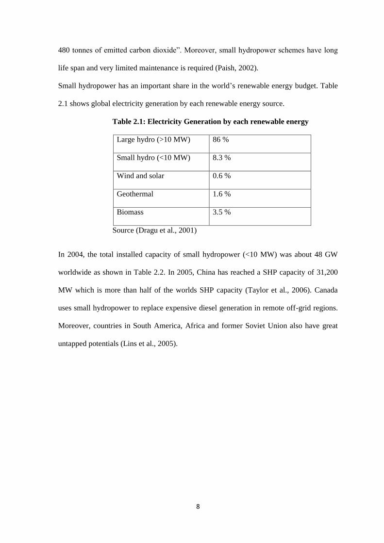
Small hydropower has an important share in the world‟s renewable energy budget. Table
2.1 shows global electricity generation by each renewable energy source.
Table 2.1: Electricity Generation by each renewable energy
Large hydro (>10 MW) 86 %
Small hydro (<10 MW) 8.3 %
Wind and solar 0.6 %
Geothermal 1.6 %
Biomass 3.5 %
Source (Dragu et al., 2001)
In 2004, the total installed capacity of small hydropower (<10 MW) was about 48 GW
worldwide as shown in Table 2.2. In 2005, China has reached a SHP capacity of 31,200
MW which is more than half of the worlds SHP capacity (Taylor et al., 2006). Canada
uses small hydropower to replace expensive diesel generation in remote off-grid regions.
Moreover, countries in South America, Africa and former Soviet Union also have great
untapped potentials (Lins et al., 2005).

9
Table 2.2: Installed SHP (<10 MW) Capacity by World Region in 2004
Region Capacity (MW) Percentage (%)
Asia 32,641 68.0
Europe 10,723 22.3
North America 2,929 6.1
South America 1,280 2.7
Africa 228 0.5
Australasia 198 0.4
Source (Taylor et al., 2006)
2.4 Hydropower and energy
Hydro power can be obtained where a flow of water falls from a higher plane to a lower
plane. This could be in a stream running down a hillside, a river over a waterfall, a weir
or from a reservoir discharge back in to a main outlet.
The amount of power available from a hydro scheme depends on the 'head' and the „flow‟
rate of the water. The head is the height difference between the inlet to the hydro turbine
and its outlet as shown in Figure 2.1
The gross head is the maximum vertical drop available to the water from the top of the
fall to the water level below. The actual head seen by a turbine is slightly less than gross
head due to losses while transferring the water into and away from the turbine, and is
therefore called the net head.
The flow rate (Q) in the water source is the volume of water passing per second.

10
Figure 2.1: Available head for Mini hydro power
This can be shown by equation 2.1.
Energy released = m g H ………….. 2.1
Where:
m = mass of water
g = gravity
H = gross head or vertical distance
The mass of the water is its density (p) multiplied by its volume (V) so that the equation
changes to:
Energy released = V ρ g H ……………. 2.2
The water enters the turbine at a rate Q value in cubic meters per second m³/s, and can be
expressed in terms of power. The S.I. unit for power is Watt.
Therefore:
Gross Power = ρ Q g H Watts ………… 2.3
Where:

11
ρ = 1000 kg/m³
g = 9.81 m/sec²
Q = volumetric flow rate m³/sec
H = gross head in meters
However the power produced by the turbine cannot equal the gross power because of
losses such as friction in pipe work and conversion machinery i.e. turbines and
generators.
A hydro turbine can have between 80% to over 90% hydraulic efficiency, although this
will reduce with size. A typical micro hydro system (<100kW) will tend to be 60% to
80% efficient.
Therefore:
Net Power = η ρ Q g H Watts ………….. 2.4
Where:
η = hydraulic efficiency of turbine
ρ = 1000 kg/m³
Q = volumetric flow rate m³/sec
g = 9.81 m/sec²
H = gross head in meters
2.5 Small hydro power component
A typical small hydro power is arranged as depicted in figure 2.2.

12
Figure 2.2: Components of Mini hydro power scheme
The principal components that are used in the MHS (Mini Hydropower System) could be
further classified into civil components, powerhouse components and transmission and
distribution networks.
2.5.1 Diversion Weir and Intake
The diversion weir depicted in figure 2.3 is a barrier built across the river and used to
divert water through an opening in the riverside (the „Intake‟ opening) into a settling
basin. Intake is the primary means of conveyance of water from the source of water in
required quantity towards the waterways of Hydro Power Project. Intake could be of side
intake type or the bottom intake type. Usually, trash racks as shown in figure 2.4 have to
be placed at the intake which acts as the filter to prevent large water borne objects to enter
the waterway of the MHP (Mini Hydro Project) (Harper, December 2011).
Forebay tank
Channel
Aqueduct Settling basin
Penstock
Power house Containing
turbine
Intake weir

13
Figure 2.3: Diversion weir
Figure 2.4: Trash rack
2.5.2 Settling Basin
Rivers generally carry high amount of sediments due to erosion activities in hills and
mountains. In order to reduce the sediments density, which have negative impact to
components of the hydropower system; de-sanding basins are used to capture sediments
by letting the particles settle by reducing the speed of the water and clearing them out
before they enter the canal. Therefore, they are usually built at the head of the canal. They
14
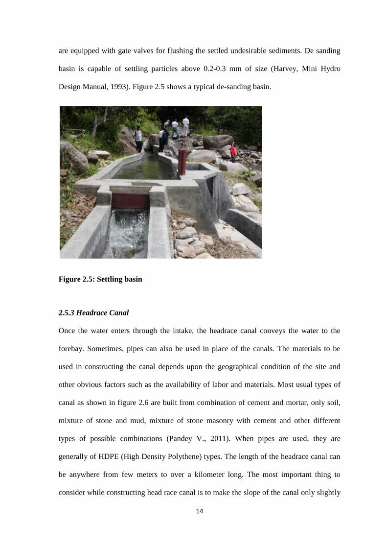
are equipped with gate valves for flushing the settled undesirable sediments. De sanding
basin is capable of settling particles above 0.2-0.3 mm of size (Harvey, Mini Hydro
Design Manual, 1993). Figure 2.5 shows a typical de-sanding basin.
Figure 2.5: Settling basin
2.5.3 Headrace Canal
Once the water enters through the intake, the headrace canal conveys the water to the
forebay. Sometimes, pipes can also be used in place of the canals. The materials to be
used in constructing the canal depends upon the geographical condition of the site and
other obvious factors such as the availability of labor and materials. Most usual types of
canal as shown in figure 2.6 are built from combination of cement and mortar, only soil,
mixture of stone and mud, mixture of stone masonry with cement and other different
types of possible combinations (Pandey V., 2011). When pipes are used, they are
generally of HDPE (High Density Polythene) types. The length of the headrace canal can
be anywhere from few meters to over a kilometer long. The most important thing to
consider while constructing head race canal is to make the slope of the canal only slightly

15
elevated because higher slope can lead to higher velocity of water which can then cause
erosion in the headrace canal surface.
Figure 2.6: Head race canal
2.5.4 Forebay
Pond at the top of a penstock or pipeline serves as final settling basin, provides
submergence of penstock inlet and accommodation of trash rack and overflow/spillway
arrangement.
Forebay tank is basically a pool at the end of headrace canal from which the penstock
pipe draws the water. The main purpose of the forebay is to reduce entry of air into the
penstock pipe, which in turn could cause cavitations (explosion of the trapped air bubbles
under high pressure) of both penstock pipes and the turbine (Masters, 2004). It is also
necessary to determine the water level at the forebay because operational head of the mini
hydro power plant is determined through this factor. A forebay again requires two sets of
additional construction. As the water speed is lowered at the forebay, it can cause
sedimentation of particles, which requires the construction of spillway as mentioned

16
before. Similarly, installation of trash racks to filter the fine sediments might be required
before the water from the forebay gets inside. Figure 2.7 illustrates a typical forebay tank.
Figure 2.7: Forebay
2.5.5 Penstock
Penstock pipes are basically close conduit pipes that help to convey the water from the
forebay tank to the turbine under pressure. The pipeline itself must be able to tolerate
sudden changes in water pressures, and to resist adequately internal and external forces,
such as the changing weather conditions for the sited area. The materials used in penstock
are usually steel, HDPE (High Density Polythene) and increasingly PVC (Poly Vinyl
Chloride).
PVC is widely used in micro-hydro because it is relatively cheap and is widely available
in a variety of sizes from 25mm to 500mm in diameter. It is suitable for high-pressure
use, has good friction loss characteristics and is corrosion resistant, but suffers from being
fragile in the respect to damage from falling rocks or trees. Mild steel is used for its
cheapness and is easily available in a wide range of diameters and pipe wall thicknesses.
It is resistant to external damage from falling rocks and trees, but when buried, it suffers

17
from long term corrosion and needs to be protected by painting or some other form of
anticorrosion coating to give an expected life of 15 years plus. Mild steel piping is heavy
but can come in convenient lengths, easier for movement and is jointed either by welding
or bolted flanges.
Penstock is one of the most important components of the MHS (Mini Hydro-power
System) because it is at this point that the potential energy of the water is converted into
kinetic energy. Due to the risk of contraction and expansion of penstock pipes due to
fluctuation in seasonal temperature, sliding type of expansion joints are placed between
two consecutive pipe lengths. Anchor block, which is basically a mass of concrete fixed
into the ground, is used to restrain the penstock from movement in undesirable directions.
Figure 2.8 depicts a mild steel penstock secured to the ground by anchor blocks.
Figure 2.8: Mild Steel Penstock

18
2.5.6 Tailrace
Tailrace is very similar to headrace canal described previously in this section. The only
difference with that of the headrace canal is that it is situated at the end of the civil
components and is used to convey the water back to the source after use in the Mini hydro
plant.
2.6 Turbines
The purpose of a turbine is to convert energy in the form of falling water into rotating
shaft power. The selection of the best turbine for any particular hydro site depends on the
site characteristics, the dominant ones being the head and flow available. Selection also
depends on the desired running speed of the generator or other device loading the turbine.
Other considerations such as whether the turbine is expected to produce power under
part-flow conditions also play an important role in the selection. All turbines have power-
speed design characteristics, as they will tend to run more efficiently at a particular speed,
head and flow combination. Turbines can be classified as high head, medium head or low
head machines.
Turbines are grouped under the following two headings: impulse turbines and reaction
turbines, as shown in the table 2.3.
Table 2.3: Turbine classification
High Head Medium Head Low Head
Impulse
Turbines
Pelton
Turgo
Multi-Jet Pelton
Cross-Flow/
Banki
Multi-Jet Pelton
Turgo
Cross-Flow/
Banki
Reaction
Turbines
Francis Propeller
Kaplan

19
2.6.1 Impulse turbines.
Impulse turbines derive their power from a jet stream striking a series of blades or
buckets as illustrated in figure 2.9. A distinct feature of an impulse turbine runner is that it
operates in air. The momentum of a high-speed water jet turns impulse turbines.
Figure 2.9: Impulse turbine
2.6.1.1 Pelton Turbine.
The Pelton wheel is probably the best known of the tangential flow impulse turbines.
Invented by a Californian mining engineer, it has changed little in the last hundred years.
It is efficient over a very wide range of flows but at lower heads the speed is a bit too low
for convenient belt drives. The Pelton wheel is used where a small flow of water is
available with a „large head‟. It resembles the waterwheels used at water mills in the past.
The Pelton wheel has small „buckets‟ all around its rim (Figure 2.10). Water from the
dam is discharged from one or more nozzles very high speed hitting the buckets, pushing
the wheel around (Figure 2.10).

20
Figure 2.10: Pelton Turbine nozzle
The buckets are split into two halves so that the central area does not act as a dead spot
incapable of deflecting water away from the oncoming jet (Figure 2.11).
Figure 2.11: Pelton Turbine bucket split into two halves
Having two or more jets enables a smaller runner to be used for a given flow and
increases the rotational speed. The required power can still be attained and the part-flow
efficiency is especially good because the wheel can be run on a reduced number of jets
with each jet in use still receiving the optimum flow.

21
Two Pelton Wheels can be placed on the same shaft either side by side or on opposite
sides of the generator (figure 2.12). This configuration is unusual and would only be used
if the number of jets per runner had already been maximized, but it allows the use of
smaller diameter and hence faster rotating runners.
Figure 2.12: Two Pelton wheels placed side by side
2.6.1.2 Turgo Turbine.
Eric Crewdson invented the Turgo impulse in 1920; it is used for heads of 12 meters or
more. The Turgo Impulse design allows a large water jet to be directed at an angled
runner blade, usually approximately 20°, giving the turbine a higher specific speed, and
therefore a smaller physical size (Figure2.13).The rugged design is particularly suited to
schemes having abrasive solids in suspension.

22
Figure 2.13: Turgo Turbine runner
Because power output from the turbine can be regulated using rapid acting deflectors
without affecting the water flow, the Turgo Impulse Turbine has been applied on many
irrigation and water treatment schemes where continuity of water flow is essential. It has
several disadvantages. Firstly it is difficult to fabricate since the buckets or vanes are
more complex in shape and overlap, it also experiences axial loading on the runner that
has to be quelled by a suitable bearing on the shaft, usually a roller bearing.
2.6.1.3 Crossflow Turbine.
In the crossflow turbine, the water in the form of a sheet is directed into the blades
tangentially at about mid way on one side. The flow of water "crosses" through the empty
centre of the turbine and exits just below the centre on the opposite side (figure 2.14).
Thus the water strikes blades on both sides of the runner.

23
Figure 2.14: Crossflow Turbine runner
It is claimed that the entry side contributes about 75% of the power extracted from the
sheet of water and that the exit side contributes the remainder. The main characteristic of
the cross-flow turbine is that it uses a broad rectangular jet of water that travels through
the turbine only once but travels across each runner blade twice, once in each direction.
This machine is therefore a turbine with two velocity stages, the water filling only part of
the runner at any one time. As far as energy utilization is concerned, the use of two
velocity stages provides no immediate advantages. The arrangement represents, however,
a very skilful design, which removes the water in a simple manner, after it has passed
through the runner without producing any backpressure. The addition of a draft tube to
the cross-flow turbine represents an idea implemented by Ossberger to enhance the
turbine's performance. Ossberger uses an air valve in the draft tube to help regulate the
head by introducing air in the draft tube.

24
Furthermore, this flow mechanism makes the turbine self-cleaning. During the first strike,
suspensions and impurities, which reach the turbine, are pressed against the blanket of the
runner. During the second strike, after a half rotation these would then be washed out.
This mechanism contributes to the long functioning period and reliability of the turbine.
They are generally built as multi-cell turbines, where the runner can be sectioned off to
allow the smaller cell to utilize small water flows and the larger cell to use medium water
flow and when both cells are opened together they utilize the full flow of the water.
(Figure 2.15)
Figure 2.15: Efficiency of Crossflow turbine at different loads

25
2.6.2 Reaction Turbines.
Reaction turbines use both velocity and pressure forces to produce power. Consequently,
large surfaces over which these forces can act are needed. Also, flow direction as the
water enters the turbine is important. They are distinguished from impulse type turbines
by having a runner that always functions within a completely water filled casing (figure
2.16). Hydrodynamic lift forces acting on the runner blades turn reaction turbines.
Figure 2.16: Reaction Turbine
2.6.2.1 Francis Turbine.
The Francis turbine is used where a large flow and a high or medium head of water is
involved. The Francis turbine is also similar to a waterwheel in that it looks like a
spinning wheel with fixed blades in between two rims. This wheel is called a „runner‟. A
circle of guide vanes surrounds the runner and controls the amount of water driving it.
Water is fed to the runner from all sides by these vanes causing it to spin. Francis turbines
are radial flow reaction turbines, with fixed runner blades and adjustable guide vanes,
used for medium heads. Francis turbines include a complex vane arrangement
surrounding the turbine itself (also called the runner) which can be seen in Figures 2.17.

26
Water is introduced around the runner through these vanes and then falls through the
runner, causing it to spin. Velocity force is applied through the vanes by causing the
water to strike the blades of the runner at an angle. Pressure forces are much more subtle
and difficult to explain, and in general, the flowing water causes pressure forces. As the
water flows across the blades, it causes a pressure drop on the back of the blades; this in
turn induces a force on the front, and along with velocity forces, causes torque.
Figure 2.17: Francis turbine assembly
Francis turbines are usually designed specifically for their intended installation; with the
complicated vane system, they are generally not used for Micro hydropower applications.
Because of their specialized design, Francis turbines are very efficient yet very costly.
2.6.2.2 Propeller.
Propeller type turbines are designed to operate where a small head of water is involved.
These turbines resemble ship‟s propellers (Figure 2.18). The basic propeller turbine

27
consists of a propeller, similar to a ship's propeller, fitted inside a continuation of the
penstock tube. The turbine shaft passes out of the tube at the point where the tube changes
direction. The propeller usually has three to six blades, three in the case of very low head
units and the water flow is regulated by static blades or swivel gates ("wicket gates") just
upstream of the propeller.
This kind of propeller turbine is known as a fixed blade axial flow turbine because the
pitch angle of the rotor blades cannot be changed. The part-flow efficiency of fixed-blade
propeller turbines tends to be very poor. However, with some of these the angle (pitch) of
the blades can be altered to suit the water flow.
The Propeller turbine in its simplest form is like a ship's propeller running in a tube. As
the water flows through the propeller rotates. Special coatings are used for increased
corrosion and abrasion resistance. For lowland and old mill sites the propeller turbine is
ideally suited since it is compact and fast running even on low heads.
Figure 2.18: Propeller Turbine
The angle of the bend can be between 30 and 90 degrees but standard layouts are either
45 or 90 degrees (Figure 2.19). A penstock can be used for higher heads up to 15 meters
and the turbine runner 'setting' can be lowered to avoid cavitations by inserting a length of
parallel tube between the bend and the turbine casting. Existing civil works associated
with old mills, navigation locks or irrigation structures often lend themselves to the

28
installation of this type of turbine. The Siphon layout is used for small turbines and axial-
flow pumps, where the unit is installed 'Over a Wall'.
Figure 2.19: Propeller turbine assembly
2.6.2.3 Kaplan.
Large-scale hydro sites make use of more sophisticated versions of the propeller turbines
(Figures 2.20). Varying the pitch of the propeller blades together with wicket gate
adjustment enables reasonable efficiency to be maintained under part flow conditions. For
good efficiency water needs to be given some swirl before entering the turbine runner,
where the swirl is absorbed by the runner and the water that emerges flows straight into
the draft tube. Methods for adding inlet swirl include the use of a set of guide vanes
mounted upstream of the runner with water spiraling into the runner through them.
Another method is to form a „snail shell‟ (Figure 2.21) housing for the runner in which
the water enters tangentially and is forced to spiral into the runner. Such turbines are
known as variable pitch or Kaplan turbines. Water flows into the turbine casing and
passes the runner blades through to the draft tube then to the tailrace .Various
configurations of Kaplan turbines exist and can be mounted horizontally, vertically or

29
angled in the same way as propeller turbines. This type of turbine has a high efficiency
over a wide range of heads and outputs and has a high specific speed.
Figure 2.20: Kaplan Turbine assembly
Figure 2.21: Kaplan Turbine components
2.6.3 Turbine Efficiency.
A significant factor in the comparison of the various turbine types is their relative
efficiencies both at their design and at reduced flows. Typical efficiency curves are shown
in Figure 2.22.

30
An important note is that the Pelton and Kaplan turbines retain very high efficiencies
when running below design flow; in contrast the efficiency of the Francis turbine falls
away more sharply if run below half their normal flow, as does the Crossflow turbine, but
the multi-celled Crossflow turbine retains a high efficiency but with a reduced output.
Most fixed pitch propeller turbines perform poorly except above 80% of full flow.
Figure 2.22: Turbine efficiency curve
2.7 Governors.
The turbine usually drives the generator through either a gearbox, through a pulley and
belt system, or directly using shock-absorbing brushes. The governor modulates the
generator speed in order to control the electrical frequency of generation. The governor
does this by detecting the change in the electrical load output of the generator, and then
altering the flow of water into the turbine using valves. They can be linked to a level
switch situated in the storage reservoir so that the flow through the turbine is also
dependent on the level, and hence the water flows. Governors can either be mechanical or
electrically operated.

31
2.8 Generators.
Generators can be either of a Synchronous or Asynchronous type. In a synchronous
generator the frequency of the electricity produced is directly related (i.e. synchronous)
with the rotational speed of the shaft. Therefore at 50 Hz generation, the shaft rotates at a
fixed sub multiple of 50Hz, depending on the gearing ratio. This type of generator must
be designed to withstand the high runaway speeds that can sometimes occur during
hydroelectric turbine system faults. They often have to be specially designed, thus
increasing their cost considerably. These generators come in single phase (for small
systems) and three phase (for larger outputs), and the single phase type is more
commonly known as an alternator. Within induction generation or asynchronous
generation a motor is used as a generator. This type of generator is simple in construction
containing fewer parts, making it cheaper and more reliable than synchronous generators.
It can withstand 200% runaway speeds without harm, and has no brushes or other parts to
require maintenance. In this type of generator power enters the grid when the speed of
rotation has a frequency greater than that of the grid. This is called slip. Usually systems
are designed for maximum power to be entering the grid at a slip of about 10%. Power is
actually drawn from the grid to provide the magnetic field until running speed is
achieved, when power is then produced. When operating in conjunction with a large
power grid, a standard single or three-phase motor may be used as a generator. Hydro
power plants designed as asynchronous installations are usually more economical than
synchronous generating sets. In the past, asynchronous plants were equipped with
minimal equipment.

32
2.9 Capacity Factor
Capacity factor is a ratio summarizing how hard a turbine is working. This is expressed as
( ) ( )
( ) ( ) ………………. 2.5
Capacity factor varies with design flows as shown in table 2.4.
Table 2.4: Design flow in relation to capacity factor
Design flow Qo Capacity Factor
Qmean 40%
0.75 Qmean 50%
0.5 Qmean 60%
0.33 Qmean 70%
2.10 Design Flow
It is not promising to have a scheme that uses significantly more than the mean river flow
since it will not be economically feasible. Therefore turbine design flow for run of the
river scheme operating with no appreciable water storage will not normally be greater
than Qmean. The greater the chosen value of the design flow, the smaller proportion of the
year that the system will be operating on full power meaning low capacity factor.
Operating at full power or high capacity factor means design flow should be less than
Qmean.

33
CHAPTER THREE
METHODOLOGY
The methodology used in this study entails the following activities: reconnaissance of the
study area, data collection of both primary and secondary data and data analysis and
preliminary design of the Mini hydro system.
3.1 Reconnaissance Survey
The purpose of the site reconnaissance was to gain understanding of the site
characteristics, site topography, flow regimes, geology of the area, access roads to the
place and nearness of transmission line. From this observation, identification of possible
location for weirs, head canal, de-silting tank, forebay and switch yard were obtained.
3.2 Primary and Secondary data
Both primary and secondary data were gathered. Primary data was collected from the
field and these were hydrological data, topographical data and geological data. Secondary
data was collected on rainfall, temperature, relative humidity and wind speed from
meteorological agency and from report and document to supplement field data.
3.3 Stream Flow Measurement
Stream velocity was measured using the float method. Measurement was taken at a place
where the axis of the streambed is straight and has fairly constant cross sectional area. A
cork was tossed from upstream of the river of known length and the time taken to traverse
that distance was noted. This sequence was repeated several times at four different
locations from the edge of the river and average time was obtained hence average
velocity. Figure 3.1 – 3.4 shows how this was done.

34
Figure 3.1: measuring stream flow using float method
Figure 3.2: measuring stream width.

35
Figure 3.3: measuring stream width.
Figure 3.4: measuring stream flow rate.

36
Table 3.1: Measuring stream flow using float method
Location from edge (m) Depth (m) Length (m) Time (s) Velocity (m/s)
0.91 0.3 5 10 0.50
1.83 0.48 5 6 0.83
1.74 0.85 5 6 0.83
3.66 0.3 5 11 0.45
Mean 0.65
Measurement of cross sectional area was made at a place where the axis of the streambed
is straight and the cross section of the river is almost uniform. The width of the river was
measured with a tape and was 5.03 meters. The depth of the river was measured at an
interval along it width and average depth calculated as shown in table 3.1. The cross
sectional area was determined by multiplying stream width by average depth of the river.
(∑
) ……………………….. 3.1
Where:
B – Stream width
h- Depth of stream
S-Cross sectional area
(
)
Stream flow was calculated using the formula
Stream discharge (m3/s) = Average Depth x Width x Average velocity
Stream discharge (m3/s) = Cross sectional area x Average velocity

37
Stream discharge (m3/s) = 2.427m
2 x 0.65m/s
= 1.58m3/s
3.4 Stream Flow Estimation
Since river Pumpum is not gauged, there is no discharge data that can be used for
planning Mini hydro power project. Since only rainfall data is available, the stream flow
was estimated using Area –Rainfall method.
Figure 3.5: Catchment area of an MHP
3.4.1 Area –Rainfall Method
The relation of rainfall, runoff (direct runoff, base runoff), and evaporation is indicated by
the viewpoint of annual water balance as shown in equation 3.2. In this case, pooling of
drainage area and inflow and runoff from/to other drainage area are not necessary.
An estimated average discharge at the considered intake point can be made from existing
precipitation records at a nearby meteorological station or a preinstalled rain gauge.
Precipitation is usually measured in mm. The total volume of rain passing through the
control point (Figure 3.5) each month is calculated by equation 3.4.

38
……………….......................................................................................... 3.2
……………………..……………….……………………………………. 3.3
( )
…………………………………………………………………….. 3.4
Where,
P: Annual rainfall (mm)
R: Annual runoff (mm)
Q: Flow rate (m3/s)
Et: Annual evaporation (mm)
Acatchment: Catchment Area (Km2)
T: Time
Consider that some of the rain does not pass through the control point, because it seeps
into the underground and drains as sub surface flow (Figure 3.6). A much larger amount
evaporates in dry and windy areas. The losses caused by seepage and evaporation are
difficult to quantify and therefore it is useful to make assumptions to be on the safe side.
Evaporation losses depend on water surfaces, irrigated surfaces and transpiring plants.
The potential evaporation losses per day from water surfaces can be calculated using the
Blaney Criddle Formula.
39
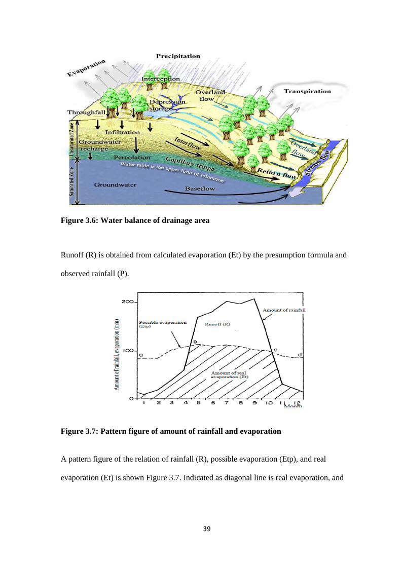
Figure 3.6: Water balance of drainage area
Runoff (R) is obtained from calculated evaporation (Et) by the presumption formula and
observed rainfall (P).
Figure 3.7: Pattern figure of amount of rainfall and evaporation
A pattern figure of the relation of rainfall (R), possible evaporation (Etp), and real
evaporation (Et) is shown Figure 3.7. Indicated as diagonal line is real evaporation, and

40
area above line b-c is river runoff including sub-surface water. Possible evaporation (a-b-
c-d) is obtained by presumption formula.
Figure 3.8: Pattern figure of runoff
(2) Direct runoff and base runoff
A pattern of annual runoff is shown Figure 3.8. The runoff is provided from sub-surface
water, and it contained base runoff with less seasonal fluctuation and direct runoff
wherein the rainfall immediately becomes the runoff. The ratio of sub-surface water to
annual runoff (R) is shown in Table 3.2. Where, Rb is sub surface water,
For Africa, Rb / R = 0.35 constant, and the base runoff is taken as constant.
Table 3.2: World Water balance model
Source: Lvovich 1973

41
Data of Japan from Ministry of Land, Infrastructure and Transport
(3) Calculation of possible evaporation
The calculation formulas are Blaney-Criddle formula, Penman formula, and Thornthwaite
formula etc. Herein, Blaney-Criddle formula was used which is the simplest method using
the longitude and temperature of the project site.
Blaney-Criddle formula is given by equation 3.5.
( )
…………………………………………………………………… 3.5
Where,
U: Monthly evaporation (mm)
K: Monthly coefficient of vegetation
P: Monthly rate of annual sunshine (%)
t: Monthly average temperature (oC)
Monthly average temperature (t) was obtained from measured temperatures at the
catchment area.
Monthly rate of annual sunshine (P) was obtained by taking the latitude of the propose
dam site (Lat. 8゜N) and selecting the appropriate P from a table in appendix E
corresponding to the selected latitude.
K value depends on the vegetation condition. Herein, a constant of 0.6 was used.
(4) Calculation of evaporation
As shown in Table 3.3; the monthly evaporations are obtained by lower value of rainfall
or possible evaporation.
(5) Computation of monthly runoff data
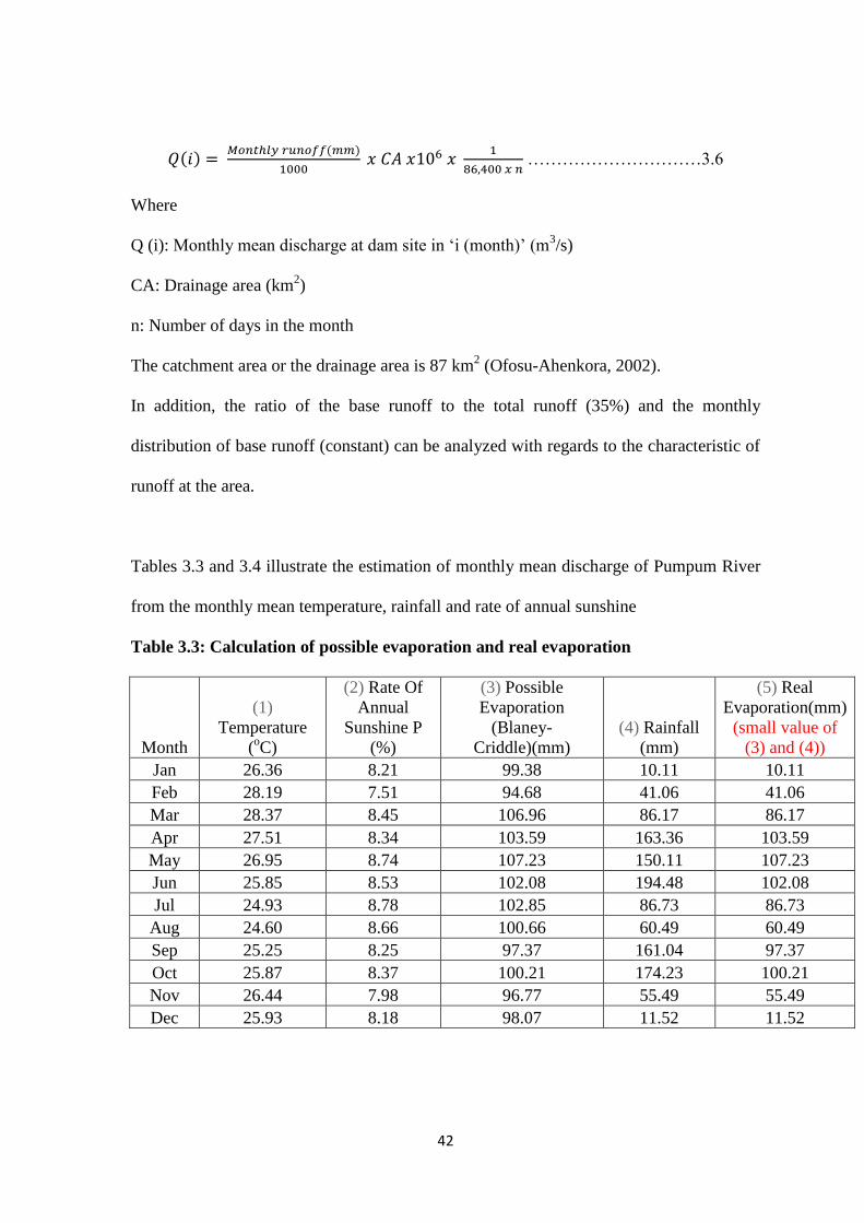
Derivation of the monthly mean discharge data at the dam site is by using equation 3.6.
42
( ) ( )
…………………………3.6
Where
Q (i): Monthly mean discharge at dam site in „i (month)‟ (m3/s)
CA: Drainage area (km2)
n: Number of days in the month
The catchment area or the drainage area is 87 km2 (Ofosu-Ahenkora, 2002).
In addition, the ratio of the base runoff to the total runoff (35%) and the monthly
distribution of base runoff (constant) can be analyzed with regards to the characteristic of
runoff at the area.
Tables 3.3 and 3.4 illustrate the estimation of monthly mean discharge of Pumpum River
from the monthly mean temperature, rainfall and rate of annual sunshine
Table 3.3: Calculation of possible evaporation and real evaporation
Month
(1)
Temperature
(oC)
(2) Rate Of
Annual
Sunshine P
(%)
(3) Possible
Evaporation
(Blaney-
Criddle)(mm)
(4) Rainfall
(mm)
(5) Real
Evaporation(mm)
(small value of
(3) and (4))
Jan 26.36 8.21 99.38 10.11 10.11
Feb 28.19 7.51 94.68 41.06 41.06
Mar 28.37 8.45 106.96 86.17 86.17
Apr 27.51 8.34 103.59 163.36 103.59
May 26.95 8.74 107.23 150.11 107.23
Jun 25.85 8.53 102.08 194.48 102.08
Jul 24.93 8.78 102.85 86.73 86.73
Aug 24.60 8.66 100.66 60.49 60.49
Sep 25.25 8.25 97.37 161.04 97.37
Oct 25.87 8.37 100.21 174.23 100.21
Nov 26.44 7.98 96.77 55.49 55.49
Dec 25.93 8.18 98.07 11.52 11.52

43
Table 3.4: Calculation of mean stream discharge
Month
(6)
Runoff(mm)
((4) -(5))
(7) Direct
Runoff(mm)
((2) x 0.65)
(8) Base
Runoff(mm)
(9) Monthly
Runoff(mm)
((7)+ (8))
(10) Monthly
mean
discharge(m3/s)
Jan 0.00 0.00 9.89 9.89 0.32
Feb 0.00 0.00 8.93 8.93 0.32
Mar 0.00 0.00 9.89 9.89 0.32
Apr 59.77 38.85 9.57 48.42 1.63
May 42.88 27.88 9.89 37.77 1.23
Jun 92.40 60.06 9.57 69.63 2.34
Jul 0.00 0.00 9.89 9.89 0.32
Aug 0.00 0.00 9.89 9.89 0.32
Sep 63.67 41.39 9.57 50.96 1.71
Oct 74.02 48.11 9.89 58.00 1.88
Nov 0.00 0.00 9.57 9.57 0.32
Dec 0.00 0.00 9.89 9.89 0.32
332.75 216.29 116.46 332.75 0.92
(Note) (8) Base runoff: distribute uniformity 332.75 ×0.35 = 116.4625 mm to each month
3.7 Measurement of Head
The head between the intake point and the power house was measured .While a surveying
level can be used for the purpose of measuring, a more simple head measuring method
using GPS device was used to determine the head. The Altitude of the intake point was
taken with the GPS receiver and noted down. Next the elevation at downstream end
where the proposed power house will be located was also taken. The measured head was
calculated by the difference in elevation of intake point and the elevation of power house.
Elevation of intake point - 292.93m
Elevation of power house point – 242m
Head = Elevation of intake point – Elevation of power house point
= 292.93m – 242m
50.93m

44
CHAPTER FOUR
RESULT AND DATA ANALYSIS
Data was collected on rainfall and temperature from the year 1992 to 2012 and was used
to estimate stream flow for the period. Table 4.1 shows the mean flow rate of Pumpum
River from the year 1992 to 2012.
Table 4.1: Monthly mean discharge of Pumpum River from 1992 to 2012
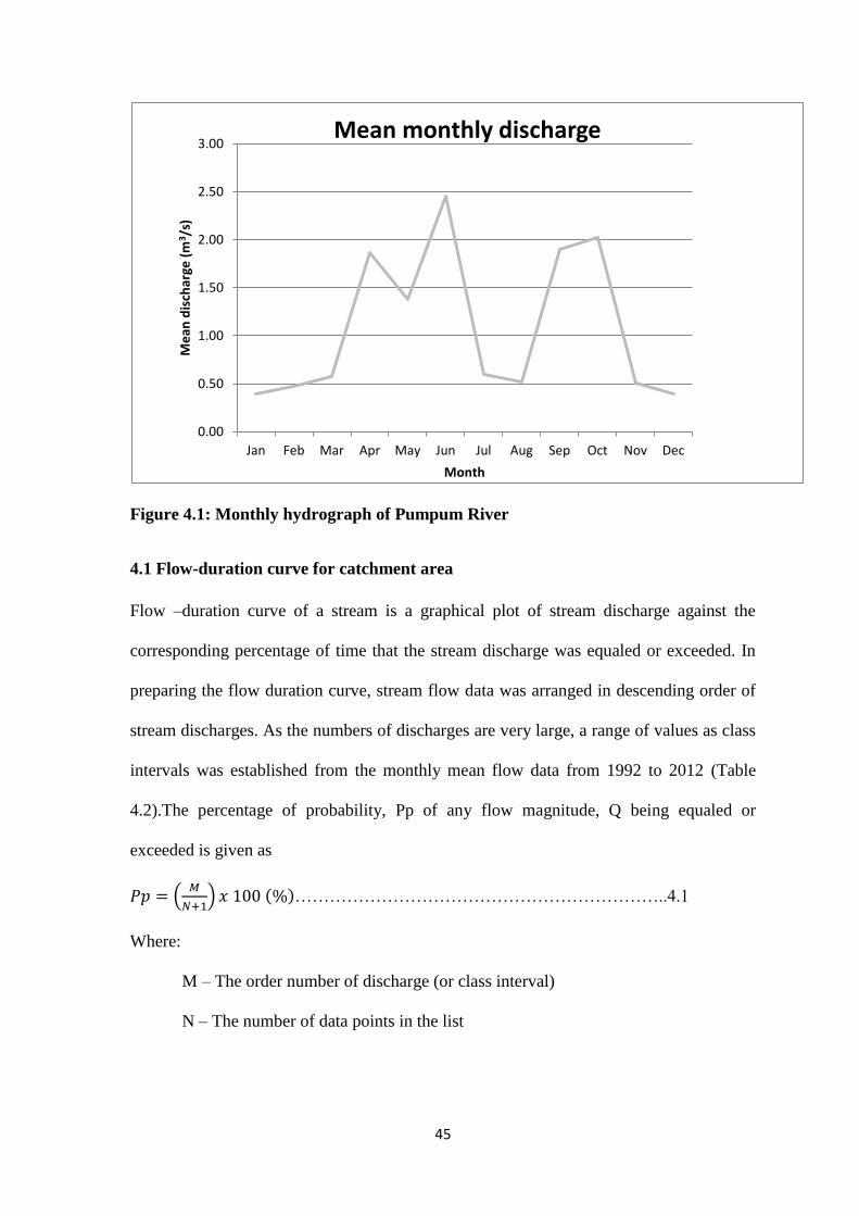
Figure 4.1 depicts the monthly average discharge or hydrograph for the past 20 years. It
shows the months with the least and highest flow rates.
Months
Year Jan Feb Mar Apr May Jun Jul Aug Sep Oct Nov Dec Mean
1992 0.39 0.39 0.39 2.25 1.46 1.39 0.39 0.39 2.73 1.20 0.39 0.39 0.98
1993 0.39 0.39 0.39 0.58 3.30 1.52 0.39 0.39 2.33 1.45 0.39 0.39 0.99
1994 0.39 0.39 0.39 0.39 0.59 1.22 0.39 0.39 2.40 3.01 0.39 0.39 0.86
1995 0.39 0.39 1.18 3.99 1.40 1.56 0.49 0.41 2.64 1.46 0.39 0.39 1.22
1996 0.39 1.94 0.39 1.09 0.52 3.07 0.93 0.91 0.39 2.23 0.39 0.39 1.05
1997 0.39 0.39 0.39 0.39 0.89 2.96 0.39 0.39 0.39 1.73 0.39 0.39 0.76
1998 0.39 0.39 0.39 1.07 0.39 2.40 0.39 0.39 1.86 3.40 0.39 0.39 0.99
1999 0.39 0.39 1.37 1.21 1.58 0.98 0.39 0.39 1.71 1.20 0.39 0.39 0.87
2000 0.39 0.39 0.39 3.45 0.39 0.89 0.39 0.79 0.39 0.39 0.49 0.39 0.73
2001 0.39 0.39 0.95 6.86 0.39 4.96 0.39 0.39 0.76 0.39 0.39 0.39 1.39
2002 0.39 0.39 0.39 3.86 1.92 1.93 0.39 0.39 0.39 1.50 0.39 0.39 1.03
2003 0.39 0.39 0.39 2.60 1.17 3.26 0.39 0.39 3.23 2.70 0.39 0.39 1.31
2004 0.39 0.39 0.39 1.16 1.88 0.39 0.39 1.03 4.40 3.62 0.39 0.39 1.24
2005 0.39 0.39 0.39 0.81 0.53 0.62 0.39 0.39 1.38 3.23 0.39 0.39 0.78
2006 0.39 0.39 0.42 0.39 2.02 3.58 0.39 0.39 0.57 3.91 0.39 0.39 1.10
2007 0.39 0.39 0.56 1.66 1.04 2.91 1.30 0.39 5.48 1.25 0.39 0.39 1.35
2008 0.39 0.39 0.39 2.62 0.94 1.97 0.39 1.51 3.05 2.26 0.39 0.39 1.23
2009 0.39 0.39 1.59 1.54 1.33 2.30 1.88 0.39 0.39 0.68 2.75 0.39 1.17
2010 0.39 0.39 0.59 2.56 1.11 4.57 1.59 0.39 1.59 1.23 0.39 0.39 1.27
2011 0.39 0.48 0.39 0.39 1.26 5.29 0.39 0.39 3.15 2.55 0.39 0.39 1.29
2012 0.39 0.39 0.39 0.39 4.92 3.78 0.39 0.39 0.61 3.17 0.39 0.39 1.30
Mean 0.39 0.47 0.58 1.87 1.38 2.45 0.59 0.52 1.90 2.03 0.51 0.39 1.09
45
Figure 4.1: Monthly hydrograph of Pumpum River
4.1 Flow-duration curve for catchment area
Flow –duration curve of a stream is a graphical plot of stream discharge against the
corresponding percentage of time that the stream discharge was equaled or exceeded. In
preparing the flow duration curve, stream flow data was arranged in descending order of
stream discharges. As the numbers of discharges are very large, a range of values as class
intervals was established from the monthly mean flow data from 1992 to 2012 (Table
4.2).The percentage of probability, Pp of any flow magnitude, Q being equaled or
exceeded is given as
(
) ( )………………………………………………………..4.1
Where:
M – The order number of discharge (or class interval)
N – The number of data points in the list
0.00
0.50
1.00
1.50
2.00
2.50
3.00
Jan Feb Mar Apr May Jun Jul Aug Sep Oct Nov Dec
Me
an d
isch
arge
(m
3 /s)
Month
Mean monthly discharge

46
Table 4.2: Monthly mean discharge and percentage probability
47
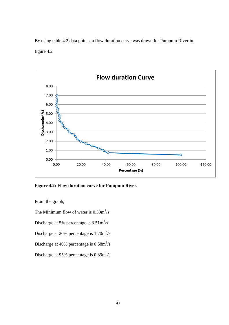
By using table 4.2 data points, a flow duration curve was drawn for Pumpum River in
figure 4.2
Figure 4.2: Flow duration curve for Pumpum River.
From the graph;
The Minimum flow of water is 0.39m3/s
Discharge at 5% percentage is 3.51m3/s
Discharge at 20% percentage is 1.70m3/s
Discharge at 40% percentage is 0.58m3/s
Discharge at 95% percentage is 0.39m3/s
0.00
1.00
2.00
3.00
4.00
5.00
6.00
7.00
8.00
0.00 20.00 40.00 60.00 80.00 100.00 120.00
Dis
char
ge(m
3/s
)
Percentage (%)
Flow duration Curve
48
4.2 Compensational Flow
Some volume of water is allowed to flow all the time so as to sustain aquatic organisms in
the stream.70 liters or 0.07m3/s is allowed for this purpose leaving 0.32m
3/s of flow
available for power generation.
4.3 Power potential
Power potential of the site is obtained from equation 4.1. The design flow obtained is
0.32m3/s which is available 95% throughout the year from the flow duration curve.
( ) ( ) ( ) ………………………………………………………..
4.2
The best turbine can have hydraulic efficiencies in the range of 80% to over 90%
although this will reduce with size. If we take 70 % (as typical water to wire efficiency
for the whole system (BHA, 2005) then the above equation simplifies to
( ) ( ) ( )….…………………………………………………….4.3
( ) ( )
( )
Energy = 114.1KW x Capacity Factor x 8760hr
= 114.1KW x 0.95 x 8760hr
= 949,540.2 KWh

49
4.3 Design of Civil structures
Based on the survey results, the preliminary design was accomplished at prefeasibility
level to determine the main specifications of the facilities and equipment.
4.3.1 Height of flood barrier walls
Height of intake barrier walls Hb is the height to which water is likely to rise in the worst
flood condition as shown in figure 4.3.
Figure 4.3: Intake barrier wall.
The characteristic discharge of a weir is given by the equation
………………………………………………………………… 4.4
Where:
Qr =River discharge (m3/s)
Cd - Coefficient of discharge for the weir
Hot – Head over top of weir (m)
Lw – Length of weir (m)
Length of weir (Lw) is the same as the width of the river = 5.03m.Mean discharge of the
stream is 1.09m3/s and the coefficient of discharge of the weir Cd = 0.6.subsituting this in
the equation the head over top of the weir is given by
Hb
Hweir
Hot

50
*
+
………………………………………………………………….. 4.5
[
]
= 0.507m
Height of the weir is assume to be 1m so the height of the flood barrier wall will be given
by
Hb = Hot + Hweir = 1m + 0.5077m = 1.5077m
4.3.2 Intake dimension
The intake behaves according to discharge equation given by
√ ( )……………………………………………………4.6
Where:
Q - Discharge through intake (m3/s)
V – Velocity of water passing through intake m/s
Cd – coefficient of discharge of intake orifice (0.6<Cd<0.8)
A – Cross sectional area of intake.
Hr – Depth of water in river channel
Hh – Depth of water in head canal

51
Figure 4.4: Side intake.
The intake dimensions are determined under two conditions; normal condition when there
is no flood and flood condition.
Normal condition
Under this condition Hh = d the depth of intake opening Hr is computed from equation.
Hweir is assumed and set to 1m during normal conditions Hot = 0
Hr (normal) = Hweir + Hot = 1.0m
√ ( )
The velocity is assumed to be 2<Vi<4 m/s. Assuming a velocity of 2m/s and coefficient
of discharge of an intake of 0.6 (assuming masonry orifice) substituting into equation 4.6,
height of intake Hh is obtained.
√ ( )
(
)
( )
( )
52
Hh = 0.434m
From
Where: Qd – Design flow = 0.32m3/s
H – Intake depth = 0.434
V -velocity of intake = 2m/s
B = 0.32/0.434x2 = 0.37m
Therefore the dimension of the side intake is 0.43m x 0.37m
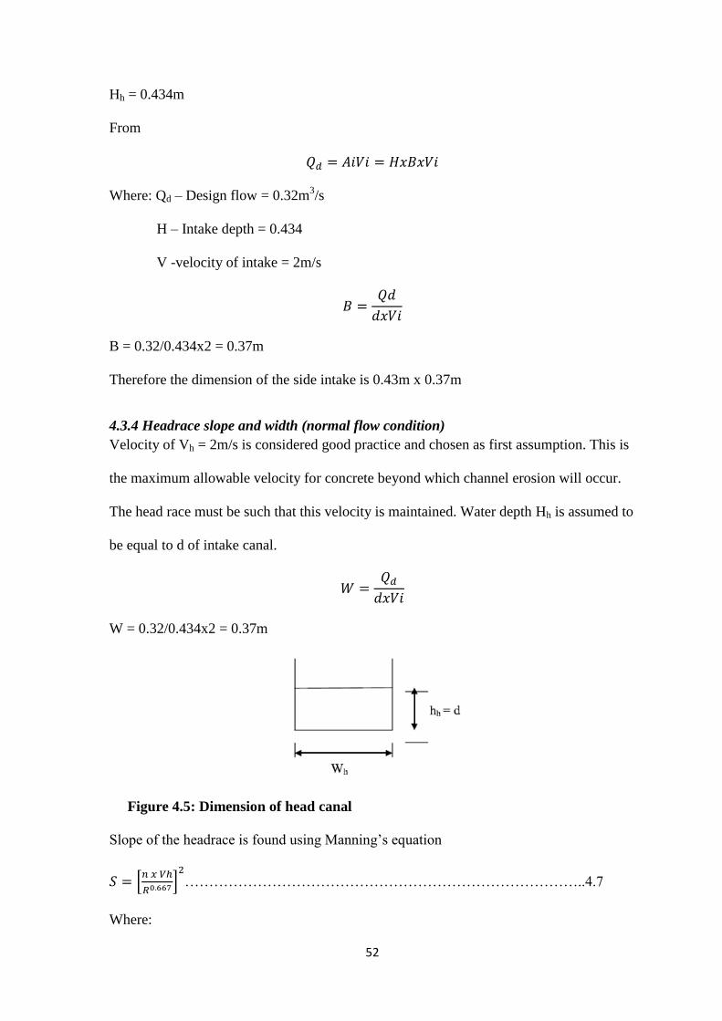
4.3.4 Headrace slope and width (normal flow condition)
Velocity of Vh = 2m/s is considered good practice and chosen as first assumption. This is
the maximum allowable velocity for concrete beyond which channel erosion will occur.
The head race must be such that this velocity is maintained. Water depth Hh is assumed to
be equal to d of intake canal.
W = 0.32/0.434x2 = 0.37m
Figure 4.5: Dimension of head canal
Slope of the headrace is found using Manning‟s equation
*
+
………………………………………………………………………..4.7
Where:
53
S = slope of the headrace
R = Wetted perimeter
n = roughness value for the material of the headrace
[
]
R = (0.37 x 0.434) / (0.37 + 2*0.434) = 0.13
[
]
S = 0.0137
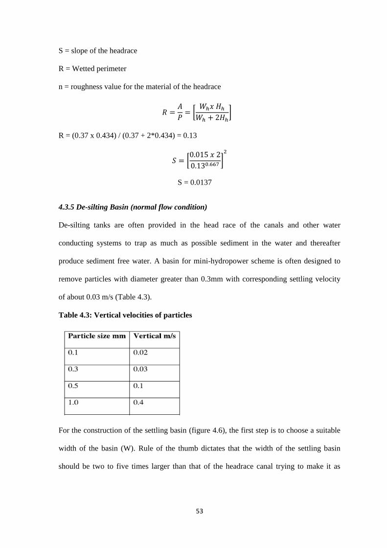
4.3.5 De-silting Basin (normal flow condition)
De-silting tanks are often provided in the head race of the canals and other water
conducting systems to trap as much as possible sediment in the water and thereafter
produce sediment free water. A basin for mini-hydropower scheme is often designed to
remove particles with diameter greater than 0.3mm with corresponding settling velocity
of about 0.03 m/s (Table 4.3).
Table 4.3: Vertical velocities of particles
For the construction of the settling basin (figure 4.6), the first step is to choose a suitable
width of the basin (W). Rule of the thumb dictates that the width of the settling basin
should be two to five times larger than that of the headrace canal trying to make it as

54
bigger as possible depending upon the available width in the MHP location (Pandey B.,
2006).
Figure 4.6: Schematic sedimentation basin
After determination of the width, the next process is to calculate the length of settling
basin (Lsettling) by using equation 4.8.
…………………………………………………………4.8
Where,
Q = design flow (m3/s)
Vvertical = fall velocity (For the settling particles of 0.3 mm diameter the fall velocity is
taken as 0.03 m/s).
By this equation the length of the settling basin is determined, but it is very important to
check at this time that the length of the settling basin is around four to ten times its width.
The width of the head race canal = 0.37m
The width of the settling basin (W) was chosen as 1.85 m which is about Five times the
width of the headrace canal and is therefore allowed.
L = 11.53m

55
Here the L/W which is 11.53/1.85 = 6.85 = 6.23 which is about 6 times the width and
therefore the width is within the range of 4-10 times the length.
4.3.7 Forebay Design
Forebay is usually designed for a live storage of 2 minutes. Stored water is utilized while
starting the turbines. The transition canal is provided for lowering the velocity gradually.
Forebay is constructed immediately before the penstock pipe and at the end of the head
race (figure 4.7). The most important element to be calculated in the design of the forebay
tank is the submergence head. The submergence head or the depth of water above
penstock pipe, should fulfill the criteria (Submergence head) hs >1.5 V2/2g
Where, V refers to the velocity of water in the penstock, which in this case is 2.5 m/s;
……………………………………………………………………4.9
hs = 0.5m
The covering water depth at the penstock inlet must be above the following value to
prevent the occurrence of inflow turbulence.
D< 1.0m -> h > 1.0d
D> 1.0m -> h > 1.0d2
Where,
h: water depth from the centre of the inlet to the lowest water level of the head tank =
covering water depth (m)
d: inner diameter of the penstock (m) which is 0.41m
According to design guidelines, the value should not be less than one times the penstock
diameter hence we assumed increase by 2 times
Hs = 2 x 0.5m = 1m
Total depth = submergence head + diameter of penstock + freeboard

56
= 1m + 0.43m + 0.5m = 1.93m
Storage period T = 30s (minimum 15s)
Size of forebay
( ) ……………………………………………………………… 4.10
( )
Volume = 8.4m3
Area of forebay
……………………………………………………………………. 4.11
Area = 9.6m2
Assume a width (W) of 2m
Length (L)
Length (L) = 4.8m
Transition length:
We assume the transition angle to be 35o
Transition length = 1.16m
Total length of forebay = 4.8m + 1.16m = 5.96m
Spillway in forebay is given by equation 4.12

57
…………………………………………………4.12
(ENTEC AG, March 2001) agrees that for a MHP, broad round edged profile where Cw =
1.6 is easy and reliable to construct. Therefore, the value of Cw taken while designing
spillway for the project is also 1.6
Hovertop = 500mm = 0.5m
Spillway length = 0.57m
Figure 4.7: Forebay dimension
4.3.8 Penstock Design
In designing the penstock, it length (L) was determined from topographic map. In this
project, the length of the penstock was 200m.Restricting head loss to 5% is considered to
be a good practice. Head loss in penstock is given by equation 4.13
………………………………………………………………… 4.13
Where:
D = Penstock diameter
h = Head loss
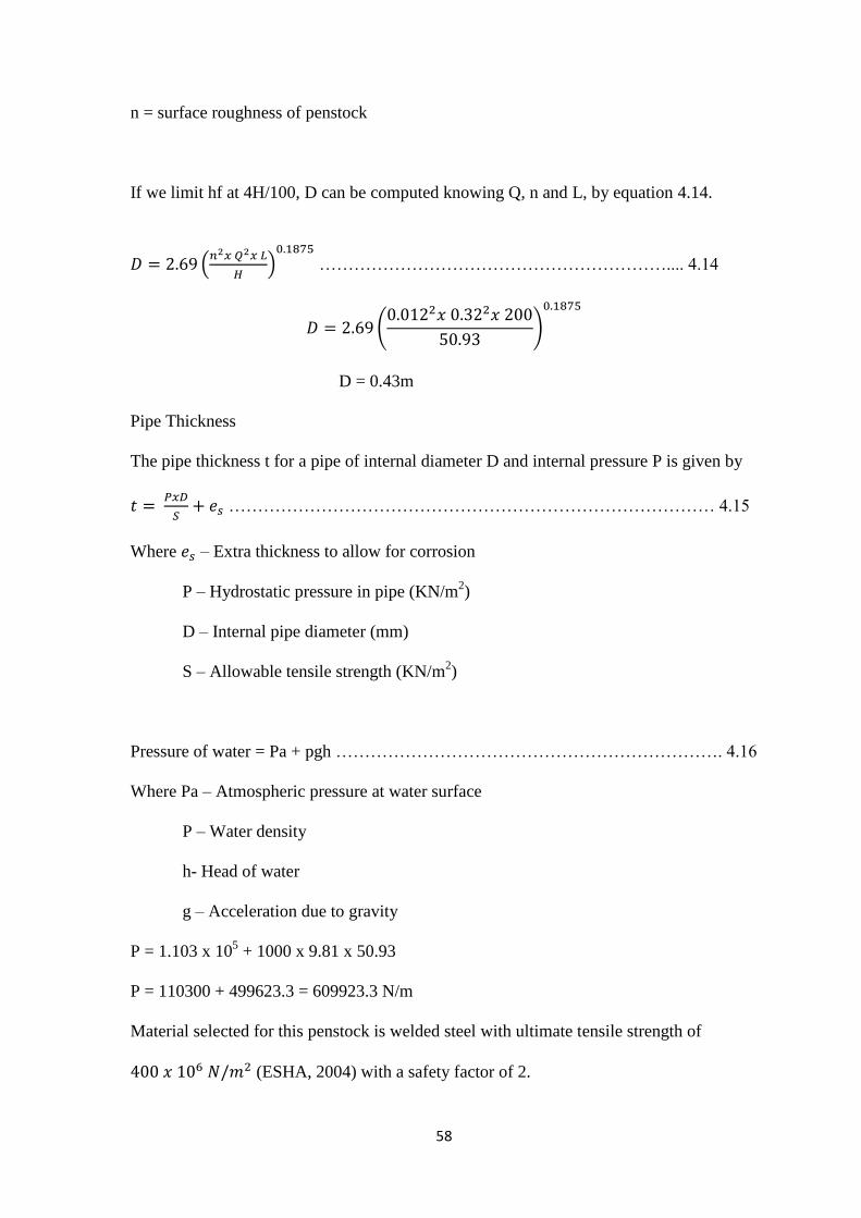
58
n = surface roughness of penstock
If we limit hf at 4H/100, D can be computed knowing Q, n and L, by equation 4.14.
(
)
…………………………………………………….... 4.14
(
)
D = 0.43m
Pipe Thickness
The pipe thickness t for a pipe of internal diameter D and internal pressure P is given by
………………………………………………………………………… 4.15
Where – Extra thickness to allow for corrosion
P – Hydrostatic pressure in pipe (KN/m2)
D – Internal pipe diameter (mm)
S – Allowable tensile strength (KN/m2)
Pressure of water = Pa + pgh …………………………………………………………. 4.16
Where Pa – Atmospheric pressure at water surface
P – Water density
h- Head of water
g – Acceleration due to gravity
P = 1.103 x 10⁵ + 1000 x 9.81 x 50.93
P = 110300 + 499623.3 = 609923.3 N/m
Material selected for this penstock is welded steel with ultimate tensile strength of
(ESHA, 2004) with a safety factor of 2.

59
T = 0.001311m + 0.001m = 0.002311m = 2.3mm
4.4 Design of Mechanical equipments
Turbine selection is based on the output of turbine and available head for the site. From
figure 4.8, the suitable turbine for this plant is Cross flow turbine.
Figure 4.8: Turbine Selection Graph
4.4.1Determination of specific speed of turbine n (rpm)
Rotational speed of the turbine is given by equation 4.18
√
………………………………………………………………………… 4.18
Net head = Gross head – Head loss
Net head = Gross head – 4% (Gross Head)
= 50.93m – (0.04x50.93) = 48.89m

60
Rotational speed of turbine = 750 rpm
√
Ns = 62
This is within the specific speed range of a cross flow turbine given as 40 < Ns < 200.
(MHP-1, 2009)
4.4.2 Cross flow runner diameter
Runner diameter of cross flow turbine is given by equation 4.19.
√
………………………………………………………….. 4.19
√
D = 0.38 m
4.4.3 Cross flow runner length
The jet thickness is usually between one tenth and one fifth of runner diameter. Having
estimated tjet, the approximate runner length Lrunner can be found from the orifice
discharge equation
√
√
√
√ …………………………………………………………….. 4.20
tjet = 1/5 x D = 0.2 x 0.38 = 0.0758
√
L = 0.139m

61
4.5 Sizing of Electrical equipments
The output of generator in KVA is calculated from the following equation
( )
…………………………………………………………. 4.21
Where H – net head
Q – Rated discharge
n – Combined efficiency of turbine, transmitter and generator
pf –power factor usually 80%
Power factor (pf) is based on the type of load in the system. However, 80% is usually
applied for convenient purpose.
( )
P (KVA) = 134
4.5.1 Speed and number of poles
The rated rotational speed is specified according to the frequency (50 or 60 Hz) of power
network and the number of poles as shown in equation 4.22 for induction generator
selected for this project.
( )
( ) …………………………………………………………….. 4.22
Where P – number of poles of generator
F – Frequency of the system (Hz)
S – Slip of generator
Slip is given by the equation
……………………………………………………………………………….
4.23
Where Ns – is the synchronous speed
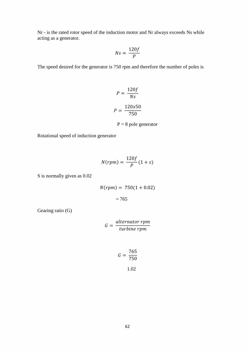
62
Nr - is the rated rotor speed of the induction motor and Nr always exceeds Ns while
acting as a generator.
The speed desired for the generator is 750 rpm and therefore the number of poles is
P = 8 pole generator
Rotational speed of induction generator
( )
( )
S is normally given as 0.02
( ) ( )
= 765
Gearing ratio (G)
1.02

63
Figure 4.9 illustrates the layout of the main components of the project on the landscape.
Table 4.4 depicts the summary of the project specifications.
Figure 4.9: Layout of the main components on site

64
Table 4.4: Summary of project technical specifications
Components Dimension/Size
Drainage Area (km2) 87
Gross head (m) 50.93
Design Discharge (m3/s) 0.32
Orifice for side intake Area – 0.37m x 0.43m
Delivery discharge – 0.32m3/s
Headrace canal Area – 0.37m x 0.43m
Wetted perimeter – 0.13m
Velocity – 2m/s
Canal bed slope – 0.0137 (1:73m)
Settling Basin Length – 11.53m
Width – 1.85m
Forebay Length -5.96m
Width -2m
Depth - 1.93m
Penstock Diameter - 0.43m
Thickness - 2.3mm
Length -250m
Turbine Crossflow -(114KW)
Specific Speed - 62
Runner diameter - 0.38m
Runner length - 0.14m
Generator
Size - 134 KVA
rotational speed -750 rpm
number of poles - 8
4.6 Economic Appraisal
The economic analysis is a comparison of cost and benefits that enables the investor(s) to
make informed choice whether to develop the project or abandon it. Small hydro cost can
be split into three segments which are: Machinery, Civil works and external costs.
Payback method was used to validate the viability of the project. The payback method

65
determines the number of years required for the invested capital to be offset by resulting
benefits. The required number of years is termed the payback, recovery, or break-even
period. The economic analysis was done using the software program RETScreen4, a clean
energy project analysis software which is provided free of charge by Natural Resources
Canada.
4.6.1 Project Costing
The Small Hydro Project Model of RETScreen software offers two methods for project
costing; the detailed costing method and the formula costing method. The costing method
is selected from the drop-down list in the beginning of Cost Analysis worksheet. The
detailed costing method will not be used in this study. The formula costing method is
based on empirical formulae that have been developed to relate project costs to key
project parameters. After selecting formula costing method for calculation of project
costs, project country should be entered (Table 4.5). The formula method uses Canadian
projects as a baseline and then allows the user to adjust the results for local conditions.
The cost of projects outside Canada compared to the cost of projects in Canada will
depend, to a great extent, on the relative cost of equipment, fuel, labour and equipment
manufacturing, and the currency of the country. For projects outside Canada, costs are
adjusted based on the relative costs of these items and the exchange rate. The ratio of the
costs of fuel and labour between Ghana and Canada for the year 2013 are examined and
the following values were found:
Canadian average diesel fuel cost was 5.1 US$/gallon and Ghana average diesel fuel cost
5.0US$/gallon. Therefore Ghana versus Canadian fuel cost ratio is calculated as 1:1.

66
Canadian versus Ghana labor cost was calculated based on the minimum wage per month.
Canada‟s minimum wage is 16,710$/Month and Ghana minimum wage is 689$/Month
(Wikipedia.com) and as such Ghana versus Canada labor cost is calculated as 0.04:1
Ghana versus Canadian equipment manufacture cost ratio is also estimated as unity since
the manufacturing sector for hydropower does not exist in Ghana and significant
percentage of the equipment needed is generally imported. The average exchange rate
between USD and CAD for the year 2013 is found as 0.98 (Bank of Canada, 2013).
The selection of project classification is an important parameter for the correct evaluation
of project costing because the costs of certain components, particularly the civil works,
are affected by this selection. This is due to larger projects requiring more conservative
designs with higher associated risks.
Table 4.5: Hydro formula costing method.
Country Ghana
Local vs. Canadian equipment cost
ratio 1.00
Local vs. Canadian fuel cost ratio 1.00
Local vs. Canadian labour cost ratio 0.04
Equipment manufacture cost coefficient 1.00
Exchange rate $/CAD 0.98
Cold climate yes/no No
Design flow m³/s 0.32 0.32
Gross head m 50.93 50.93
Number of turbines turbine 1 1
Type Cross-flow Cross-flow
Flow per turbine m³/s 0.32
Turbine runner diameter per unit m 0.29
Facility type Mini Micro
Existing dam yes/no No
New dam crest length m 1
Rock at dam site yes/no Yes
Maximum hydraulic losses % 4.0% 4.0%
Miscellaneous losses % 2.0%

67
Based on the hydro costing method, the initial cost of the project was estimated as
$395,000 breaks down as follows (Table 4.6).
Table 4.6: Cost categorization of project.
Amount Adjustment
factor
Amount Relative
costs Initial costs (credits) $ $
Feasibility study 12,000 1.00 12,000 3.0%
Development 15,000 1.00 15,000 3.8%
Engineering 75,000 1.00 75,000 19.0%
Power system
Hydro turbine 118,000 1.00 118,000 29.9%
Road construction 0 1.00 0 0.0%
Transmission line 4,000 1.00 4,000 1.0%
Substation 4,000 1.00 4,000 1.0%
Balance of system &
miscellaneous
Penstock 104,000 1.00 104,000 26.3%
Canal 2,000 1.00 2,000 0.5%
Tunnel 0 1.00 0 0.0%
Other 61,000 1.00 61,000 15.4%
Sub-total: 167,000 167,000
Total initial costs 395,000 395,000 100.0%
4.6.2 Retscreen – Energy Model and Power Project General Entries
RETScreen project information entries are list below. Items in bold refer to RETScreen
field name, and items in normal font were entered by the user. Note that descriptions of
some of the more obscure fields are given below it.
Analysis Type: Method 1
Proposed Project: Run-of -river
Gross Head: 50.93 (m)
Maximum Tail water Effect: 0.00 (m)
Residual Flow: 0.070 (m3/s)
Percent Time Firm Flow Available: 95 (%)
Design Flow: 0.32 (m3/s)
Turbine Type: Cross-flow

68
Turbine Efficiency: Standard
Number of Turbines: 1
Efficiency Adjustment: 0.0 (%)
Flow Values (m3/s) for the Flow Duration Curve (FDC): 1992-2012 estimated average
Flow Data (m3/s) were used
Maximum Hydraulic Losses: 4 (%)
Miscellaneous Losses: 2 (%)
Generator Efficiency: 89 (%)
Availability: 95 (%)
(This represents about 18 days of equivalent down time per year.)
Electricity Export Rate: 0.1 Dollars ($) per kilowatt hour (kWh), or 100 dollars
per megawatt hour ($/MWh)
Total Initial Cost: 395,000 ($)
O&M Parts and Labour: 10,000 ($)
Fuel Cost Escalation Rate: 0 (%)
Inflation Rate: 9.0 (%) (Bank of Ghana, 2010)
Project Life: 25 (yrs)
Debt Ratio: 70 (%)
(This is the amount of money borrowed compared with the money used).
Debt Interest Rate: 20 (%)
Debt Term: 15 (yrs)
(This is the length of time that debt is being paid on the project).

69
Table 4.7: Financial summary of project.
Financial viability
Pre-tax IRR - equity % 43.4%
Pre-tax IRR - assets % 21.3%
Simple payback yr 4.9
Equity payback yr 3.2
Cumulative cash flows graph
Cu
mu
lati
ve
cash
flo
ws
($)
Year
Figure 4.10: Cumulative cash flow graph
The project is feasible according to RETScreen-Small Hydro Model as the net present
value and internal rate of return are positive and the benefit cost ratio is above 1 which is
shown in Figure 4.10. The simple payback is after 4.9 years.
-1,000,000
0
1,000,000
2,000,000
3,000,000
4,000,000
5,000,000
6,000,000
7,000,000
0 1 2 3 4 5 6 7 8 9 10 11 12 13 14 15 16 17 18 19 20 21 22 23 24 25

70
CHAPTER FIVE
CONCLUSIONS AND RECOMMENDATIONS
5.1 Conclusions
The summary of the main findings based on the analysis undertaken in chapters is
presented in this section followed by key recommendations.
Stream flow rate and head of Pumpum river
Adequate head and flow are necessary requirements for hydropower
generation (ESHA, 2004). Pumpum River has a potential for
producing electricity. The available head measured was 50.93m.
Pumpum River is perennial as it has some flow at all times of the
year. There is a guarantee flow rate of 0.32m3/s throughout the
year. The designed flow obtained in this work is 0.32m3/s which is
available 95 percentage of the time and gives a power of 114 KW.
Preliminary design of small hydro power plant.
Preliminary design of the hydropower plant was carried out. Cross
flow turbine was selected since it meets both head and power
requirements which can be produced by the plant and also maintains
appreciable efficiency at low flow rate. The turbine was sized to produce
power output of 114kW with a runner diameter of 380mm and a runner
length of 140mm.An 8 poles Induction motor was used as the preferred
generator with a rated power of 134KVA and a rotational speed of
750rpm.
The following civil work components were designed: Weir and
intake, headrace, spillway, de-silting tank, forebay tank and

71
penstock. The dimension of the side intake is 0.37m x 0.43m
allowing a delivery of 0.32m3/s discharge into the headrace canal.
Headrace canal have a size of 0.37m x 0.43m with a bed slope of
0.0137.Settling basin has the following dimensions: Length -11.53m,
Width-1.85m.Forebay has the following dimensions: Length – 5.96m,
Width -2m, Depth – 1.93m.The penstock material selected is welded steel
with the following dimensions: Diameter -430mm,thickness -2.3mm and
length of 250m
Economical Appraisals of Kintampo mini hydropower plant
RETScreen module was used to analyze the economic viability of the
hydropower project. From the module, the simple payback of 4.9 years
was obtained. Initial cost of the project was $ 395,000 and estimated
annual revenue of $ 90,830.
Modeling of RETScreen module
RETScreen module was used to analyze the viability of the project.
The outputs calculated from this module were: Maximum hydraulic
losses (4%), power capacity (106 KW), Capacity factor (95%) and
electricity exported to grid (880MWh).The result of the experiment
compares favorably with the result of RETScreen. Whiles 114 KW was
obtained from the experiment as the power produced, 106 KW was
estimated by the RETScreen Software. This means the software value is
93% of the experimental value. For the annual energy delivered to the grid,
experimental result gave 950MWh whiles RETScreen gave annual energy
delivered to the grid as 880 MWh. This value is 93% of the experimental
result. The proposed project will bring benefits such as no atmospheric

72
pollutants and minimal green house gases emission; enhance air quality,
minimized depleting non-renewable fuel resources and slowing down
climate change. Proposed small hydropower plant will be
sustainable and can be implemented.
5.2 Recommendations.
The project is found to be technically attractive, financially sound and
environmentally friendly. The key recommendations can be summarized as follows:
i. The in- situ and laboratory test of rock and soil type at project site is
recommended to get further geo-technical properties of rock and soil in details.
ii. It is recommended to carry out detail investigation of flood hazards around
proposed project site.
iii. The catchment area needs to be estimated using GIS software such as ArcGIS.
iv. It is recommended that the river be gauged for at least a year for accurate
discharge information before any serious hydropower development.

73
REFERENCES
Anderson, T. D (1999), Rural Energy Services, A handbook for stainable energy
development, Intermediate Technology Development Group (ITDG), London
BHA (2005), A guide to UK mini-hydro developments. British Hydropower
Association.
Boustani, F (2009), An Assessment of the Small Hydropower Potential of Sisakht
Region of Yasuj, World Academy of Science, Engineering and Technology 57 2009
Christian Arduser, Leif Karcheter (2009), Civil Works for micro hydro power units,
Institute of civil engineering, University of Applied sciences, Northwestern Switzerland.
ESHA (2004), Guide on how to develop a small hydro plant
D. Bashir (2009), Hydrological Studies for small Hydropower planning. National Water
Resources Institute, Kaduna
Eri A. Boye (2011), A feasibility and economic study into the use of micro hydro power
applications to generate electricity from the Victoria Capital Regional District’s
municipal water facility, Victoria, British Columbia, Canada. Msc Thesis, University of
Iceland
Emmanuel Mwangomo (2010), Proposing sustainable small hydro power for rural
setting, Msc thesis University of Dar es Salaam.

74
Fritz, J. J (1984), Small and Mini Hydropower Systems , McGraw-Hill Book
Company, New York
Gordon, N. D, McMahon TA, Finlayson B.L, Gippel G.J, Nathan R.J,( 2004). Stream
Hydrology - An introduction for ecologists. 2nd Edition, Wiley
Google Earth, www.google earth
Hauer, F.R and Lambert', G. (1996), Methods in stream ecology. Academic Press.
Jayanta, K. G (2009), Geospatial Technology - its applications in small
Hydro Power Project, A paper presented at international training course on
small hydro
JICA (2003), MHP-1 Manual for Design, Implementation and Management for Micro-
hydropower volume 1.
Karekezi, S and Kimarii J (2005), "The potential contribution of non -
electrified renewable energy technologies for poverty reduction in east
Africa"
Klaus Jorde (2009), Good and Bad of Mini Hydro Power, the ASEAN Center of Energy
(ACE)
Mohibullah, M. A. (2004), Basic Design Aspects of Micro Hydro Power Plant and Its

75
Potential Development in Malaysia, National Power & Energy Conference
(PECon) 2004 Proceedings, KualaLumpur, Malaysia.
Ministerial conference on water for Agriculture and energy in Africa (2008). Hydro
Power Resource Assessment of Africa.
Orzan Korkmaz (2007), A case study of feasibility assessment of small hydropower
scheme, Middle East Technical University.
Pushpa Chitrakar (2005), Micro – Hydropower Design Aids Manual, Version 2005.10,
Small Hydropower promotion project GTZ.
Ramos H (2000), Guidelines for design of small hydropower plants-, Department of
Economic Development, Belfast, North Ireland.
Robert Bass (2009). Hydroelectric Feasibility Study. An assessment of the feasibility of
generating power using storm water in Oregon City.
RET Screen International (2010), Clean Energy Project Analysis Software. Natural
Resources Canada Ottawa.
Sarkar, S and Gundekar, H. G (2007), Geomorphologic Parameters: Are they
Indicators for Installation of a Hydropower Site, International Conference on Small
Hydropower - Hydro Sri Lanka, 22-24 October 2007.
Standards/Manuals/guidelines for small hydro development (2008), Ministry of New and

76
Renewable Energy, Government of India
Sven Dernedde, A.K. Ofosu-Ahenkorah (2002). Mini Hydro Power in Ghana Prospects
and Challenges. Energy Foundation, Ghana.
TEA (2004), World Energy Outlook-, International Energy Agency, Paris,
France.Wamukonya,N (2001), Renewable Energy Technologies in Africa,
UNEP Collaborating Centre on Energy and Environment.
Wazed, M.A and Ahmed, S (2008), Micro Hydro Energy Resources in Bangladesh, A
Review. Australian Journal of Basic and Applied Sciences . 2(4):1209-1222, 2008
TSSN 1991-8178 .0 2008, ENSTnei Publication.
Younis A. G (1996), Use of a GIS in reconnaissance studies for small -scale
hydro power development in a developing country: a case study of Tanzania-.
Proceedings of the Vienna conference, April 1996. TAHS Publ. no. 235, 1996
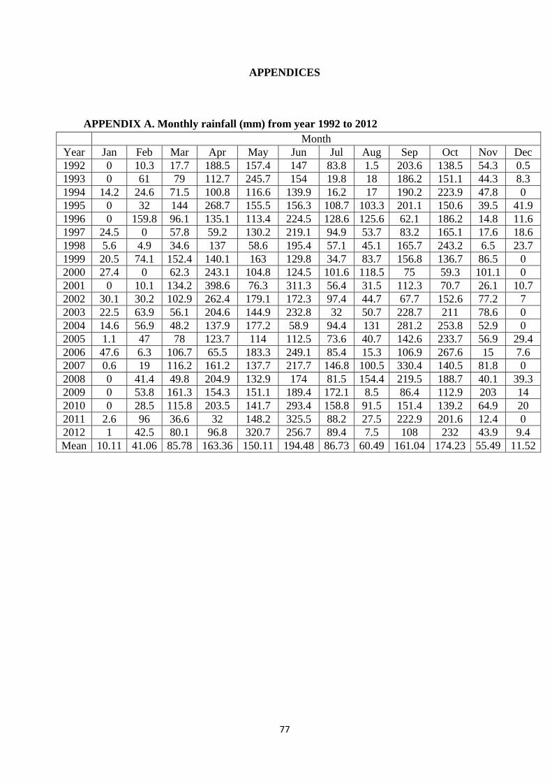
77
APPENDICES
APPENDIX A. Monthly rainfall (mm) from year 1992 to 2012
Month
Year Jan Feb Mar Apr May Jun Jul Aug Sep Oct Nov Dec
1992 0 10.3 17.7 188.5 157.4 147 83.8 1.5 203.6 138.5 54.3 0.5
1993 0 61 79 112.7 245.7 154 19.8 18 186.2 151.1 44.3 8.3
1994 14.2 24.6 71.5 100.8 116.6 139.9 16.2 17 190.2 223.9 47.8 0
1995 0 32 144 268.7 155.5 156.3 108.7 103.3 201.1 150.6 39.5 41.9
1996 0 159.8 96.1 135.1 113.4 224.5 128.6 125.6 62.1 186.2 14.8 11.6
1997 24.5 0 57.8 59.2 130.2 219.1 94.9 53.7 83.2 165.1 17.6 18.6
1998 5.6 4.9 34.6 137 58.6 195.4 57.1 45.1 165.7 243.2 6.5 23.7
1999 20.5 74.1 152.4 140.1 163 129.8 34.7 83.7 156.8 136.7 86.5 0
2000 27.4 0 62.3 243.1 104.8 124.5 101.6 118.5 75 59.3 101.1 0
2001 0 10.1 134.2 398.6 76.3 311.3 56.4 31.5 112.3 70.7 26.1 10.7
2002 30.1 30.2 102.9 262.4 179.1 172.3 97.4 44.7 67.7 152.6 77.2 7
2003 22.5 63.9 56.1 204.6 144.9 232.8 32 50.7 228.7 211 78.6 0
2004 14.6 56.9 48.2 137.9 177.2 58.9 94.4 131 281.2 253.8 52.9 0
2005 1.1 47 78 123.7 114 112.5 73.6 40.7 142.6 233.7 56.9 29.4
2006 47.6 6.3 106.7 65.5 183.3 249.1 85.4 15.3 106.9 267.6 15 7.6
2007 0.6 19 116.2 161.2 137.7 217.7 146.8 100.5 330.4 140.5 81.8 0
2008 0 41.4 49.8 204.9 132.9 174 81.5 154.4 219.5 188.7 40.1 39.3
2009 0 53.8 161.3 154.3 151.1 189.4 172.1 8.5 86.4 112.9 203 14
2010 0 28.5 115.8 203.5 141.7 293.4 158.8 91.5 151.4 139.2 64.9 20
2011 2.6 96 36.6 32 148.2 325.5 88.2 27.5 222.9 201.6 12.4 0
2012 1 42.5 80.1 96.8 320.7 256.7 89.4 7.5 108 232 43.9 9.4
Mean 10.11 41.06 85.78 163.36 150.11 194.48 86.73 60.49 161.04 174.23 55.49 11.52
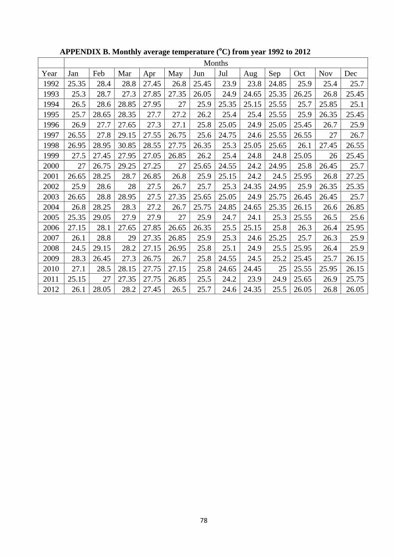
78
APPENDIX B. Monthly average temperature (oC) from year 1992 to 2012
Months
Year Jan Feb Mar Apr May Jun Jul Aug Sep Oct Nov Dec
1992 25.35 28.4 28.8 27.45 26.8 25.45 23.9 23.8 24.85 25.9 25.4 25.7
1993 25.3 28.7 27.3 27.85 27.35 26.05 24.9 24.65 25.35 26.25 26.8 25.45
1994 26.5 28.6 28.85 27.95 27 25.9 25.35 25.15 25.55 25.7 25.85 25.1
1995 25.7 28.65 28.35 27.7 27.2 26.2 25.4 25.4 25.55 25.9 26.35 25.45
1996 26.9 27.7 27.65 27.3 27.1 25.8 25.05 24.9 25.05 25.45 26.7 25.9
1997 26.55 27.8 29.15 27.55 26.75 25.6 24.75 24.6 25.55 26.55 27 26.7
1998 26.95 28.95 30.85 28.55 27.75 26.35 25.3 25.05 25.65 26.1 27.45 26.55
1999 27.5 27.45 27.95 27.05 26.85 26.2 25.4 24.8 24.8 25.05 26 25.45
2000 27 26.75 29.25 27.25 27 25.65 24.55 24.2 24.95 25.8 26.45 25.7
2001 26.65 28.25 28.7 26.85 26.8 25.9 25.15 24.2 24.5 25.95 26.8 27.25
2002 25.9 28.6 28 27.5 26.7 25.7 25.3 24.35 24.95 25.9 26.35 25.35
2003 26.65 28.8 28.95 27.5 27.35 25.65 25.05 24.9 25.75 26.45 26.45 25.7
2004 26.8 28.25 28.3 27.2 26.7 25.75 24.85 24.65 25.35 26.15 26.6 26.85
2005 25.35 29.05 27.9 27.9 27 25.9 24.7 24.1 25.3 25.55 26.5 25.6
2006 27.15 28.1 27.65 27.85 26.65 26.35 25.5 25.15 25.8 26.3 26.4 25.95
2007 26.1 28.8 29 27.35 26.85 25.9 25.3 24.6 25.25 25.7 26.3 25.9
2008 24.5 29.15 28.2 27.15 26.95 25.8 25.1 24.9 25.5 25.95 26.4 25.9
2009 28.3 26.45 27.3 26.75 26.7 25.8 24.55 24.5 25.2 25.45 25.7 26.15
2010 27.1 28.5 28.15 27.75 27.15 25.8 24.65 24.45 25 25.55 25.95 26.15
2011 25.15 27 27.35 27.75 26.85 25.5 24.2 23.9 24.9 25.65 26.9 25.75
2012 26.1 28.05 28.2 27.45 26.5 25.7 24.6 24.35 25.5 26.05 26.8 26.05

79
APPENDIX C. Estimated monthly discharge (m3/s) of Pumpum River from year
1992 to 2012
Year
Rainfa
ll
Temperat
ure
Annual
Sunshine
Possible
Evaporati
on
(Blaney-
Criddle)
Real
Evapora
tion Runoff
Direct
Runoff
Base
Runof
f
Month
ly
Runof
f
Mont
hly
mean
disch
arge
Jan-92 0 25.35 8.21 97.12 0.00 0.00 0.00 12.12 12.12 0.39
Feb-92 10.3 28.4 7.51 95.12 10.30 0.00 0.00 10.95 10.95 0.39
Mar-92 17.7 28.8 8.45 107.95 17.70 0.00 0.00 12.12 12.12 0.39
Apr-92 188.5 27.45 8.34 103.46 103.46 85.04 55.28 11.73 67.01 2.25
May-92 157.4 26.8 8.74 106.86 106.86 50.54 32.85 12.12 44.97 1.46
Jun-92 147 25.45 8.53 101.14 101.14 45.86 29.81 11.73 41.54 1.39
Jul-92 83.8 23.9 8.78 100.37 83.80 0.00 0.00 12.12 12.12 0.39
Aug-92 1.5 23.8 8.66 98.76 1.50 0.00 0.00 12.12 12.12 0.39
Sep-92 203.6 24.85 8.25 96.46 96.46 107.14 69.64 11.73 81.37 2.73
Oct-92 138.5 25.9 8.37 100.27 100.27 38.23 24.85 12.12 36.97 1.20
Nov-92 54.3 25.4 7.98 94.50 54.30 0.00 0.00 11.73 11.73 0.39
Dec-92 0.5 25.7 8.18 97.55 0.50 0.00 0.00 12.12 12.12 0.39
Jan-93 0 25.3 8.21 97.00 0.00 0.00 0.00 12.12 12.12 0.39
Feb-93 61 28.7 7.51 95.73 61.00 0.00 0.00 10.95 10.95 0.39
Mar-93 79 27.3 8.45 104.47 79.00 0.00 0.00 12.12 12.12 0.39
Apr-93 112.7 27.85 8.34 104.37 104.37 8.33 5.41 11.73 17.15 0.58
May-93 245.7 27.35 8.74 108.18 108.18 137.52 89.39 12.12 101.51 3.30
Jun-93 154 26.05 8.53 102.54 102.54 51.46 33.45 11.73 45.18 1.52
Jul-93 19.8 24.9 8.78 102.77 19.80 0.00 0.00 12.12 12.12 0.39
Aug-93 18 24.65 8.66 100.78 18.00 0.00 0.00 12.12 12.12 0.39
Sep-93 186.2 25.35 8.25 97.59 97.59 88.61 57.60 11.73 69.33 2.33
Oct-93 151.1 26.25 8.37 101.07 101.07 50.03 32.52 12.12 44.64 1.45
Nov-93 44.3 26.8 7.98 97.57 44.30 0.00 0.00 11.73 11.73 0.39
Dec-93 8.3 25.45 8.18 96.99 8.30 0.00 0.00 12.12 12.12 0.39
Jan-94 14.2 26.5 8.21 99.70 14.20 0.00 0.00 12.12 12.12 0.39
Feb-94 24.6 28.6 7.51 95.53 24.60 0.00 0.00 10.95 10.95 0.39
Mar-94 71.5 28.85 8.45 108.06 71.50 0.00 0.00 12.12 12.12 0.39
Apr-94 100.8 27.95 8.34 104.60 100.80 0.00 0.00 11.73 11.73 0.39
May-94 116.6 27 8.74 107.34 107.34 9.26 6.02 12.12 18.14 0.59
Jun-94 139.9 25.9 8.53 102.19 102.19 37.71 24.51 11.73 36.25 1.22
Jul-94 16.2 25.35 8.78 103.86 16.20 0.00 0.00 12.12 12.12 0.39
Aug-94 17 25.15 8.66 101.96 17.00 0.00 0.00 12.12 12.12 0.39
Sep-94 190.2 25.55 8.25 98.04 98.04 92.16 59.90 11.73 71.63 2.40
Oct-94 223.9 25.7 8.37 99.81 99.81 124.09 80.66 12.12 92.78 3.01
Nov-94 47.8 25.85 7.98 95.49 47.80 0.00 0.00 11.73 11.73 0.39
Dec-94 0 25.1 8.18 96.20 0.00 0.00 0.00 12.12 12.12 0.39
Jan-95 0 25.7 8.21 97.90 0.00 0.00 0.00 12.12 12.12 0.39
Feb-95 32 28.65 7.51 95.63 32.00 0.00 0.00 10.95 10.95 0.39
Mar-95 144 28.35 8.45 106.91 106.91 37.09 24.11 12.12 36.23 1.18

80
Apr-95 268.7 27.7 8.34 104.03 104.03 164.67 107.04 11.73 118.77 3.99
May-95 155.5 27.2 8.74 107.82 107.82 47.68 30.99 12.12 43.12 1.40
Jun-95 156.3 26.2 8.53 102.89 102.89 53.41 34.72 11.73 46.45 1.56
Jul-95 108.7 25.4 8.78 103.98 103.98 4.72 3.07 12.12 15.19 0.49
Aug-95 103.3 25.4 8.66 102.56 102.56 0.74 0.48 12.12 12.61 0.41
Sep-95 201.1 25.55 8.25 98.04 98.04 103.06 66.99 11.73 78.72 2.64
Oct-95 150.6 25.9 8.37 100.27 100.27 50.33 32.71 12.12 44.84 1.46
Nov-95 39.5 26.35 7.98 96.58 39.50 0.00 0.00 11.73 11.73 0.39
Dec-95 41.9 25.45 8.18 96.99 41.90 0.00 0.00 12.12 12.12 0.39
Jan-96 0 26.9 8.21 100.61 0.00 0.00 0.00 12.12 12.12 0.39
Feb-96 159.8 27.7 7.51 93.67 93.67 66.13 42.98 10.95 53.93 1.94
Mar-96 96.1 27.65 8.45 105.28 96.10 0.00 0.00 12.12 12.12 0.39
Apr-96 135.1 27.3 8.34 103.11 103.11 31.99 20.79 11.73 32.52 1.09
May-96 113.4 27.1 8.74 107.58 107.58 5.82 3.78 12.12 15.91 0.52
Jun-96 224.5 25.8 8.53 101.95 101.95 122.55 79.66 11.73 91.39 3.07
Jul-96 128.6 25.05 8.78 103.14 103.14 25.46 16.55 12.12 28.67 0.93
Aug-96 125.6 24.9 8.66 101.37 101.37 24.23 15.75 12.12 27.87 0.91
Sep-96 62.1 25.05 8.25 96.91 62.10 0.00 0.00 11.73 11.73 0.39
Oct-96 186.2 25.45 8.37 99.24 99.24 86.96 56.53 12.12 68.65 2.23
Nov-96 14.8 26.7 7.98 97.35 14.80 0.00 0.00 11.73 11.73 0.39
Dec-96 11.6 25.9 8.18 97.99 11.60 0.00 0.00 12.12 12.12 0.39
Jan-97 24.5 26.55 8.21 99.82 24.50 0.00 0.00 12.12 12.12 0.39
Feb-97 0 27.8 7.51 93.88 0.00 0.00 0.00 10.95 10.95 0.39
Mar-97 57.8 29.15 8.45 108.76 57.80 0.00 0.00 12.12 12.12 0.39
Apr-97 59.2 27.55 8.34 103.68 59.20 0.00 0.00 11.73 11.73 0.39
May-97 130.2 26.75 8.74 106.74 106.74 23.46 15.25 12.12 27.37 0.89
Jun-97 219.1 25.6 8.53 101.49 101.49 117.61 76.45 11.73 88.18 2.96
Jul-97 94.9 24.75 8.78 102.41 94.90 0.00 0.00 12.12 12.12 0.39
Aug-97 53.7 24.6 8.66 100.66 53.70 0.00 0.00 12.12 12.12 0.39
Sep-97 83.2 25.55 8.25 98.04 83.20 0.00 0.00 11.73 11.73 0.39
Oct-97 165.1 26.55 8.37 101.76 101.76 63.34 41.17 12.12 53.29 1.73
Nov-97 17.6 27 7.98 98.01 17.60 0.00 0.00 11.73 11.73 0.39
Dec-97 18.6 26.7 8.18 99.79 18.60 0.00 0.00 12.12 12.12 0.39
Jan-98 5.6 26.95 8.21 100.72 5.60 0.00 0.00 12.12 12.12 0.39
Feb-98 4.9 28.95 7.51 96.25 4.90 0.00 0.00 10.95 10.95 0.39
Mar-98 34.6 30.85 8.45 112.70 34.60 0.00 0.00 12.12 12.12 0.39
Apr-98 137 28.55 8.34 105.97 105.97 31.03 20.17 11.73 31.90 1.07
May-98 58.6 27.75 8.74 109.14 58.60 0.00 0.00 12.12 12.12 0.39
Jun-98 195.4 26.35 8.53 103.24 103.24 92.16 59.90 11.73 71.64 2.40
Jul-98 57.1 25.3 8.78 103.74 57.10 0.00 0.00 12.12 12.12 0.39
Aug-98 45.1 25.05 8.66 101.73 45.10 0.00 0.00 12.12 12.12 0.39
Sep-98 165.7 25.65 8.25 98.27 98.27 67.43 43.83 11.73 55.56 1.86
Oct-98 243.2 26.1 8.37 100.73 100.73 142.47 92.61 12.12 104.73 3.40
Nov-98 6.5 27.45 7.98 98.99 6.50 0.00 0.00 11.73 11.73 0.39
Dec-98 23.7 26.55 8.18 99.45 23.70 0.00 0.00 12.12 12.12 0.39

81
Jan-99 20.5 27.5 8.21 101.96 20.50 0.00 0.00 12.12 12.12 0.39
Feb-99 74.1 27.45 7.51 93.16 74.10 0.00 0.00 10.95 10.95 0.39
Mar-99 152.4 27.95 8.45 105.98 105.98 46.42 30.17 12.12 42.30 1.37
Apr-99 140.1 27.05 8.34 102.54 102.54 37.56 24.41 11.73 36.15 1.21
May-99 163 26.85 8.74 106.98 106.98 56.02 36.41 12.12 48.54 1.58
Jun-99 129.8 26.2 8.53 102.89 102.89 26.91 17.49 11.73 29.22 0.98
Jul-99 34.7 25.4 8.78 103.98 34.70 0.00 0.00 12.12 12.12 0.39
Aug-99 83.7 24.8 8.66 101.13 83.70 0.00 0.00 12.12 12.12 0.39
Sep-99 156.8 24.8 8.25 96.34 96.34 60.46 39.30 11.73 51.03 1.71
Oct-99 136.7 25.05 8.37 98.32 98.32 38.38 24.95 12.12 37.07 1.20
Nov-99 86.5 26 7.98 95.82 86.50 0.00 0.00 11.73 11.73 0.39
Dec-99 0 25.45 8.18 96.99 0.00 0.00 0.00 12.12 12.12 0.39
Jan-00 27.4 27 8.21 100.83 27.40 0.00 0.00 12.12 12.12 0.39
Feb-00 0 26.75 7.51 91.72 0.00 0.00 0.00 10.95 10.95 0.39
Mar-00 62.3 29.25 8.45 108.99 62.30 0.00 0.00 12.12 12.12 0.39
Apr-00 243.1 27.25 8.34 103.00 103.00 140.10 91.07 11.73 102.80 3.45
May-00 104.8 27 8.74 107.34 104.80 0.00 0.00 12.12 12.12 0.39
Jun-00 124.5 25.65 8.53 101.60 101.60 22.90 14.88 11.73 26.62 0.89
Jul-00 101.6 24.55 8.78 101.93 101.60 0.00 0.00 12.12 12.12 0.39
Aug-00 118.5 24.2 8.66 99.71 99.71 18.79 12.21 12.12 24.34 0.79
Sep-00 75 24.95 8.25 96.68 75.00 0.00 0.00 11.73 11.73 0.39
Oct-00 59.3 25.8 8.37 100.04 59.30 0.00 0.00 12.12 12.12 0.39
Nov-00 101.1 26.45 7.98 96.80 96.80 4.30 2.79 11.73 14.53 0.49
Dec-00 0 25.7 8.18 97.55 0.00 0.00 0.00 12.12 12.12 0.39
Jan-01 0 26.65 8.21 100.04 0.00 0.00 0.00 12.12 12.12 0.39
Feb-01 10.1 28.25 7.51 94.81 10.10 0.00 0.00 10.95 10.95 0.39
Mar-01 134.2 28.7 8.45 107.72 107.72 26.48 17.21 12.12 29.34 0.95
Apr-01 398.6 26.85 8.34 102.08 102.08 296.52 192.74 11.73 204.47 6.86
May-01 76.3 26.8 8.74 106.86 76.30 0.00 0.00 12.12 12.12 0.39
Jun-01 311.3 25.9 8.53 102.19 102.19 209.11 135.92 11.73 147.66 4.96
Jul-01 56.4 25.15 8.78 103.38 56.40 0.00 0.00 12.12 12.12 0.39
Aug-01 31.5 24.2 8.66 99.71 31.50 0.00 0.00 12.12 12.12 0.39
Sep-01 112.3 24.5 8.25 95.67 95.67 16.63 10.81 11.73 22.54 0.76
Oct-01 70.7 25.95 8.37 100.39 70.70 0.00 0.00 12.12 12.12 0.39
Nov-01 26.1 26.8 7.98 97.57 26.10 0.00 0.00 11.73 11.73 0.39
Dec-01 10.7 27.25 8.18 101.02 10.70 0.00 0.00 12.12 12.12 0.39
Jan-02 30.1 25.9 8.21 98.35 30.10 0.00 0.00 12.12 12.12 0.39
Feb-02 30.2 28.6 7.51 95.53 30.20 0.00 0.00 10.95 10.95 0.39
Mar-02 102.9 28 8.45 106.09 102.90 0.00 0.00 12.12 12.12 0.39
Apr-02 262.4 27.5 8.34 103.57 103.57 158.83 103.24 11.73 114.97 3.86
May-02 179.1 26.7 8.74 106.62 106.62 72.48 47.11 12.12 59.23 1.92
Jun-02 172.3 25.7 8.53 101.72 101.72 70.58 45.88 11.73 57.61 1.93
Jul-02 97.4 25.3 8.78 103.74 97.40 0.00 0.00 12.12 12.12 0.39
Aug-02 44.7 24.35 8.66 100.06 44.70 0.00 0.00 12.12 12.12 0.39
Sep-02 67.7 24.95 8.25 96.68 67.70 0.00 0.00 11.73 11.73 0.39

82
Oct-02 152.6 25.9 8.37 100.27 100.27 52.33 34.01 12.12 46.14 1.50
Nov-02 77.2 26.35 7.98 96.58 77.20 0.00 0.00 11.73 11.73 0.39
Dec-02 7 25.35 8.18 96.76 7.00 0.00 0.00 12.12 12.12 0.39
Jan-03 22.5 26.65 8.21 100.04 22.50 0.00 0.00 12.12 12.12 0.39
Feb-03 63.9 28.8 7.51 95.94 63.90 0.00 0.00 10.95 10.95 0.39
Mar-03 56.1 28.95 8.45 108.30 56.10 0.00 0.00 12.12 12.12 0.39
Apr-03 204.6 27.5 8.34 103.57 103.57 101.03 65.67 11.73 77.40 2.60
May-03 144.9 27.35 8.74 108.18 108.18 36.72 23.87 12.12 35.99 1.17
Jun-03 232.8 25.65 8.53 101.60 101.60 131.20 85.28 11.73 97.01 3.26
Jul-03 32 25.05 8.78 103.14 32.00 0.00 0.00 12.12 12.12 0.39
Aug-03 50.7 24.9 8.66 101.37 50.70 0.00 0.00 12.12 12.12 0.39
Sep-03 228.7 25.75 8.25 98.49 98.49 130.21 84.63 11.73 96.37 3.23
Oct-03 211 26.45 8.37 101.53 101.53 109.47 71.15 12.12 83.28 2.70
Nov-03 78.6 26.45 7.98 96.80 78.60 0.00 0.00 11.73 11.73 0.39
Dec-03 0 25.7 8.18 97.55 0.00 0.00 0.00 12.12 12.12 0.39
Jan-04 14.6 26.8 8.21 100.38 14.60 0.00 0.00 12.12 12.12 0.39
Feb-04 56.9 28.25 7.51 94.81 56.90 0.00 0.00 10.95 10.95 0.39
Mar-04 48.2 28.3 8.45 106.79 48.20 0.00 0.00 12.12 12.12 0.39
Apr-04 137.9 27.2 8.34 102.88 102.88 35.02 22.76 11.73 34.49 1.16
May-04 177.2 26.7 8.74 106.62 106.62 70.58 45.88 12.12 58.00 1.88
Jun-04 58.9 25.75 8.53 101.84 58.90 0.00 0.00 11.73 11.73 0.39
Jul-04 94.4 24.85 8.78 102.65 94.40 0.00 0.00 12.12 12.12 0.39
Aug-04 131 24.65 8.66 100.78 100.78 30.22 19.65 12.12 31.77 1.03
Sep-04 281.2 25.35 8.25 97.59 97.59 183.61 119.35 11.73 131.08 4.40
Oct-04 253.8 26.15 8.37 100.84 100.84 152.96 99.42 12.12 111.54 3.62
Nov-04 52.9 26.6 7.98 97.13 52.90 0.00 0.00 11.73 11.73 0.39
Dec-04 0 26.85 8.18 100.13 0.00 0.00 0.00 12.12 12.12 0.39
Jan-05 1.1 25.35 8.21 97.12 1.10 0.00 0.00 12.12 12.12 0.39
Feb-05 47 29.05 7.51 96.45 47.00 0.00 0.00 10.95 10.95 0.39
Mar-05 78 27.9 8.45 105.86 78.00 0.00 0.00 12.12 12.12 0.39
Apr-05 123.7 27.9 8.34 104.49 104.49 19.21 12.49 11.73 24.22 0.81
May-05 114 27 8.74 107.34 107.34 6.66 4.33 12.12 16.45 0.53
Jun-05 112.5 25.9 8.53 102.19 102.19 10.31 6.70 11.73 18.44 0.62
Jul-05 73.6 24.7 8.78 102.29 73.60 0.00 0.00 12.12 12.12 0.39
Aug-05 40.7 24.1 8.66 99.47 40.70 0.00 0.00 12.12 12.12 0.39
Sep-05 142.6 25.3 8.25 97.48 97.48 45.12 29.33 11.73 41.06 1.38
Oct-05 233.7 25.55 8.37 99.47 99.47 134.23 87.25 12.12 99.37 3.23
Nov-05 56.9 26.5 7.98 96.91 56.90 0.00 0.00 11.73 11.73 0.39
Dec-05 29.4 25.6 8.18 97.32 29.40 0.00 0.00 12.12 12.12 0.39
Jan-06 47.6 27.15 8.21 101.17 47.60 0.00 0.00 12.12 12.12 0.39
Feb-06 6.3 28.1 7.51 94.50 6.30 0.00 0.00 10.95 10.95 0.39
Mar-06 106.7 27.65 8.45 105.28 105.28 1.42 0.92 12.12 13.04 0.42
Apr-06 65.5 27.85 8.34 104.37 65.50 0.00 0.00 11.73 11.73 0.39
May-06 183.3 26.65 8.74 106.50 106.50 76.80 49.92 12.12 62.04 2.02
Jun-06 249.1 26.35 8.53 103.24 103.24 145.86 94.81 11.73 106.54 3.58

83
Jul-06 85.4 25.5 8.78 104.22 85.40 0.00 0.00 12.12 12.12 0.39
Aug-06 15.3 25.15 8.66 101.96 15.30 0.00 0.00 12.12 12.12 0.39
Sep-06 106.9 25.8 8.25 98.61 98.61 8.29 5.39 11.73 17.12 0.57
Oct-06 267.6 26.3 8.37 101.19 101.19 166.41 108.17 12.12 120.29 3.91
Nov-06 15 26.4 7.98 96.69 15.00 0.00 0.00 11.73 11.73 0.39
Dec-06 7.6 25.95 8.18 98.11 7.60 0.00 0.00 12.12 12.12 0.39
Jan-07 0.6 26.1 8.21 98.80 0.60 0.00 0.00 12.12 12.12 0.39
Feb-07 19 28.8 7.51 95.94 19.00 0.00 0.00 10.95 10.95 0.39
Mar-07 116.2 29 8.45 108.41 108.41 7.79 5.06 12.12 17.19 0.56
Apr-07 161.2 27.35 8.34 103.23 103.23 57.97 37.68 11.73 49.41 1.66
May-07 137.7 26.85 8.74 106.98 106.98 30.72 19.97 12.12 32.09 1.04
Jun-07 217.7 25.9 8.53 102.19 102.19 115.51 75.08 11.73 86.82 2.91
Jul-07 146.8 25.3 8.78 103.74 103.74 43.06 27.99 12.12 40.11 1.30
Aug-07 100.5 24.6 8.66 100.66 100.50 0.00 0.00 12.12 12.12 0.39
Sep-07 330.4 25.25 8.25 97.36 97.36 233.04 151.47 11.73 163.21 5.48
Oct-07 140.5 25.7 8.37 99.81 99.81 40.69 26.45 12.12 38.57 1.25
Nov-07 81.8 26.3 7.98 96.47 81.80 0.00 0.00 11.73 11.73 0.39
Dec-07 0 25.9 8.18 97.99 0.00 0.00 0.00 12.12 12.12 0.39
Jan-08 0 24.5 8.21 95.20 0.00 0.00 0.00 12.12 12.12 0.39
Feb-08 41.4 29.15 7.51 96.66 41.40 0.00 0.00 10.95 10.95 0.39
Mar-08 49.8 28.2 8.45 106.56 49.80 0.00 0.00 12.12 12.12 0.39
Apr-08 204.9 27.15 8.34 102.77 102.77 102.13 66.38 11.73 78.12 2.62
May-08 132.9 26.95 8.74 107.22 107.22 25.68 16.69 12.12 28.82 0.94
Jun-08 174 25.8 8.53 101.95 101.95 72.05 46.83 11.73 58.56 1.97
Jul-08 81.5 25.1 8.78 103.26 81.50 0.00 0.00 12.12 12.12 0.39
Aug-08 154.4 24.9 8.66 101.37 101.37 53.03 34.47 12.12 46.59 1.51
Sep-08 219.5 25.5 8.25 97.93 97.93 121.57 79.02 11.73 90.75 3.05
Oct-08 188.7 25.95 8.37 100.39 100.39 88.31 57.40 12.12 69.53 2.26
Nov-08 40.1 26.4 7.98 96.69 40.10 0.00 0.00 11.73 11.73 0.39
Dec-08 39.3 25.9 8.18 97.99 39.30 0.00 0.00 12.12 12.12 0.39
Jan-09 0 28.3 8.21 103.76 0.00 0.00 0.00 12.12 12.12 0.39
Feb-09 53.8 26.45 7.51 91.10 53.80 0.00 0.00 10.95 10.95 0.39
Mar-09 161.3 27.3 8.45 104.47 104.47 56.83 36.94 12.12 49.06 1.59
Apr-09 154.3 26.75 8.34 101.86 101.86 52.44 34.09 11.73 45.82 1.54
May-09 151.1 26.7 8.74 106.62 106.62 44.48 28.91 12.12 41.03 1.33
Jun-09 189.4 25.8 8.53 101.95 101.95 87.45 56.84 11.73 68.57 2.30
Jul-09 172.1 24.55 8.78 101.93 101.93 70.17 45.61 12.12 57.73 1.88
Aug-09 8.5 24.5 8.66 100.42 8.50 0.00 0.00 12.12 12.12 0.39
Sep-09 86.4 25.2 8.25 97.25 86.40 0.00 0.00 11.73 11.73 0.39
Oct-09 112.9 25.45 8.37 99.24 99.24 13.66 8.88 12.12 21.00 0.68
Nov-09 203 25.7 7.98 95.16 95.16 107.84 70.10 11.73 81.83 2.75
Dec-09 14 26.15 8.18 98.56 14.00 0.00 0.00 12.12 12.12 0.39
Jan-10 0 27.1 8.21 101.06 0.00 0.00 0.00 12.12 12.12 0.39
Feb-10 28.5 28.5 7.51 95.32 28.50 0.00 0.00 10.95 10.95 0.39
Mar-10 115.8 28.15 8.45 106.44 106.44 9.36 6.08 12.12 18.21 0.59

84
Apr-10 203.5 27.75 8.34 104.14 104.14 99.36 64.58 11.73 76.31 2.56
May-10 141.7 27.15 8.74 107.70 107.70 34.00 22.10 12.12 34.22 1.11
Jun-10 293.4 25.8 8.53 101.95 101.95 191.45 124.44 11.73 136.17 4.57
Jul-10 158.8 24.65 8.78 102.17 102.17 56.63 36.81 12.12 48.93 1.59
Aug-10 91.5 24.45 8.66 100.30 91.50 0.00 0.00 12.12 12.12 0.39
Sep-10 151.4 25 8.25 96.80 96.80 54.60 35.49 11.73 47.22 1.59
Oct-10 139.2 25.55 8.37 99.47 99.47 39.73 25.83 12.12 37.95 1.23
Nov-10 64.9 25.95 7.98 95.71 64.90 0.00 0.00 11.73 11.73 0.39
Dec-10 20 26.15 8.18 98.56 20.00 0.00 0.00 12.12 12.12 0.39
Jan-11 2.6 25.15 8.21 96.67 2.60 0.00 0.00 12.12 12.12 0.39
Feb-11 96 27 7.51 92.23 92.23 3.77 2.45 10.95 13.40 0.48
Mar-11 36.6 27.35 8.45 104.59 36.60 0.00 0.00 12.12 12.12 0.39
Apr-11 32 27.75 8.34 104.14 32.00 0.00 0.00 11.73 11.73 0.39
May-11 148.2 26.85 8.74 106.98 106.98 41.22 26.79 12.12 38.92 1.26
Jun-11 325.5 25.5 8.53 101.25 101.25 224.25 145.76 11.73 157.49 5.29
Jul-11 88.2 24.2 8.78 101.09 88.20 0.00 0.00 12.12 12.12 0.39
Aug-11 27.5 23.9 8.66 99.00 27.50 0.00 0.00 12.12 12.12 0.39
Sep-11 222.9 24.9 8.25 96.57 96.57 126.33 82.11 11.73 93.85 3.15
Oct-11 201.6 25.65 8.37 99.70 99.70 101.90 66.24 12.12 78.36 2.55
Nov-11 12.4 26.9 7.98 97.79 12.40 0.00 0.00 11.73 11.73 0.39
Dec-11 0 25.75 8.18 97.66 0.00 0.00 0.00 12.12 12.12 0.39
Jan-12 1 26.1 8.21 98.80 1.00 0.00 0.00 12.12 12.12 0.39
Feb-12 42.5 28.05 7.51 94.40 42.50 0.00 0.00 10.95 10.95 0.39
Mar-12 80.1 28.2 8.45 106.56 80.10 0.00 0.00 12.12 12.12 0.39
Apr-12 96.8 27.45 8.34 103.46 96.80 0.00 0.00 11.73 11.73 0.39
May-12 320.7 26.5 8.74 106.14 106.14 214.56 139.46 12.12 151.59 4.92
Jun-12 256.7 25.7 8.53 101.72 101.72 154.98 100.74 11.73 112.47 3.78
Jul-12 89.4 24.6 8.78 102.05 89.40 0.00 0.00 12.12 12.12 0.39
Aug-12 7.5 24.35 8.66 100.06 7.50 0.00 0.00 12.12 12.12 0.39
Sep-12 108 25.5 8.25 97.93 97.93 10.07 6.55 11.73 18.28 0.61
Oct-12 232 26.05 8.37 100.62 100.62 131.38 85.40 12.12 97.52 3.17
Nov-12 43.9 26.8 7.98 97.57 43.90 0.00 0.00 11.73 11.73 0.39
Dec-12 9.4 26.05 8.18 98.33 9.40 0.00 0.00 12.12 12.12 0.39

85
APPENDIX D. RETScreen Formula costing method Empirical formulas
There are 15 categorized formulae in the RETScreen-Small Hydro Model
Software to estimate the initial cost of a small hydropower project based on the
input data.The items and the corresponding formulae are listed in Table 4.5
according to the
classification of the project.1

86

87
APPENDIX E. Monthly rate of annual sunshine (Northern Hemisphere) (%)
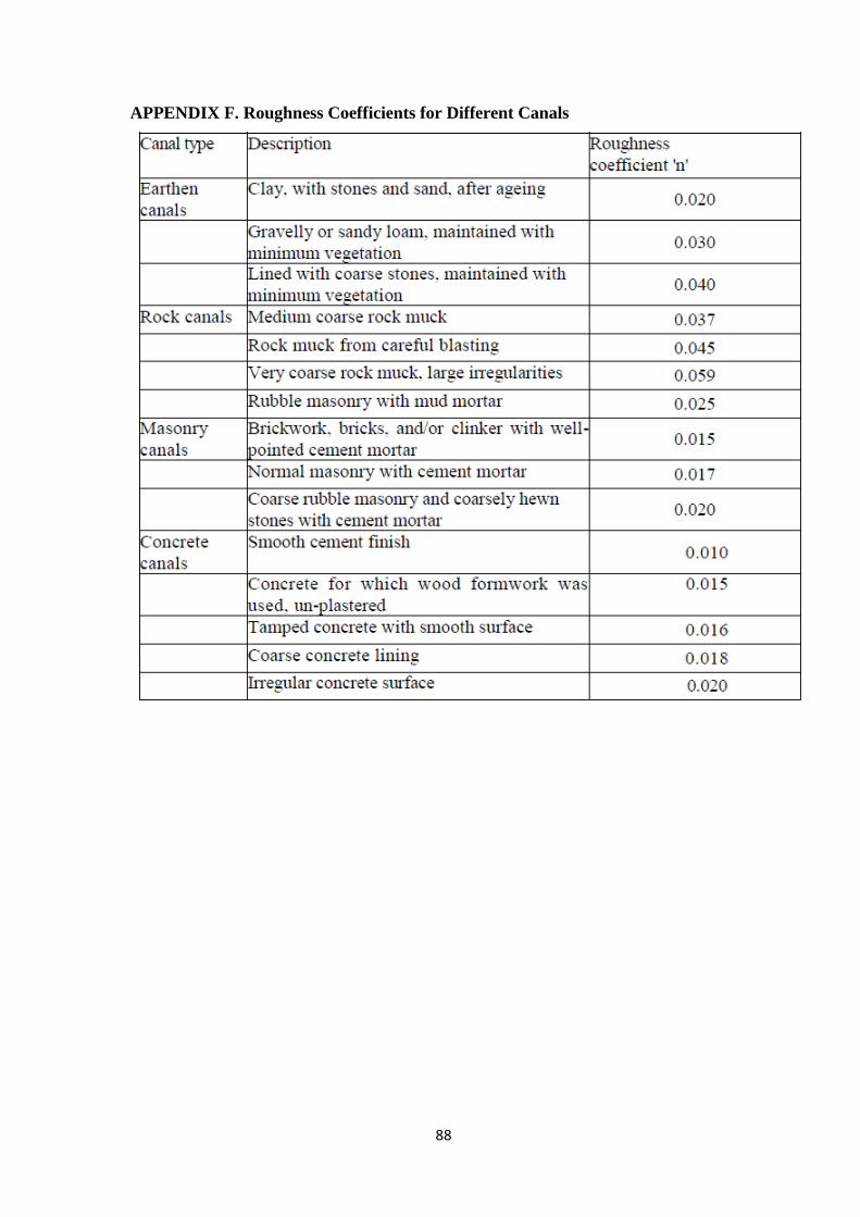
88
APPENDIX F. Roughness Coefficients for Different Canals
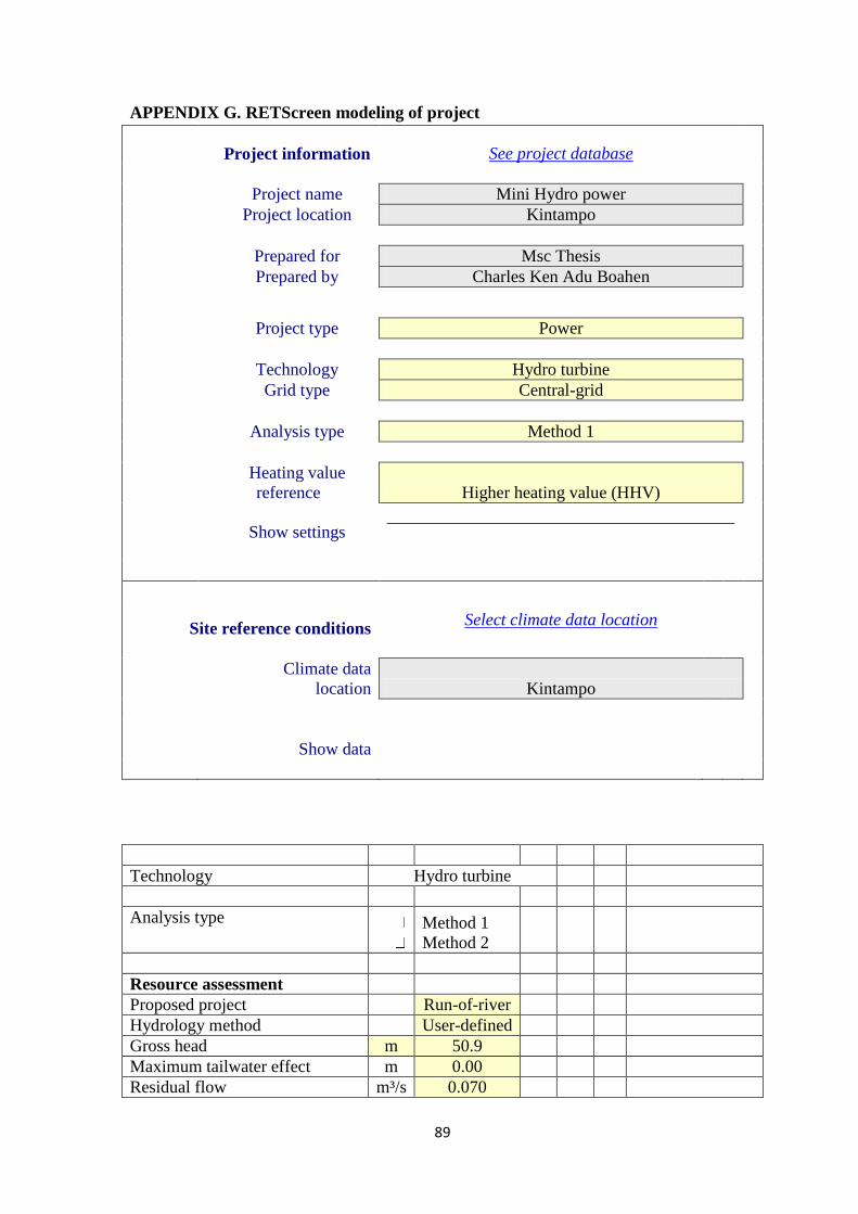
89
APPENDIX G. RETScreen modeling of project
Project information See project database
Project name Mini Hydro power
Project location Kintampo
Prepared for Msc Thesis
Prepared by Charles Ken Adu Boahen
Project type Power
Technology Hydro turbine
Grid type Central-grid
Analysis type Method 1
Heating value
reference Higher heating value (HHV)
Show settings
Site reference conditions Select climate data location
Climate data
location Kintampo
Show data
Technology Hydro turbine
Analysis type
Method 1
Method 2
Hydro turbine
Resource assessment
Proposed project Run-of-river
Hydrology method User-defined
Gross head m 50.9
Maximum tailwater effect m 0.00
Residual flow m³/s 0.070

90
Percent time firm flow available % 95.0%
Firm flow m³/s 0.45
Hydro turbine
Design flow m³/s 0.320 $ 395,000
Type Cross-flow
Turbine efficiency Standard
Number of turbines 1
Manufacturer Canyon Hydro
Model Cross-flow
Efficiency adjustment % 0.0%
Turbine peak efficiency % 0.0%
Flow at peak efficiency m³/s 0.0
Turbine efficiency at design flow % 79.0%
Flow Turbine
efficiency
Turbine
efficiency
Number
of
turbines
Combined
efficiency % m³/s
0% 5.56 0.00 0.00 0 0.00
5% 3.80 0.00 0.00 1 0.00
10% 3.10 0.34 0.34 1 0.34
15% 2.56 0.52 0.52 1 0.52
20% 1.97 0.61 0.61 1 0.61
25% 1.69 0.65 0.65 1 0.65
30% 1.43 0.68 0.68 1 0.68
35% 1.17 0.69 0.69 1 0.69
40% 0.86 0.70 0.70 1 0.70
45% 0.74 0.71 0.71 1 0.71
50% 0.71 0.71 0.71 1 0.71
55% 0.69 0.72 0.72 1 0.72
60% 0.67 0.73 0.73 1 0.73
65% 0.65 0.74 0.74 1 0.74
70% 0.63 0.74 0.74 1 0.74
75% 0.61 0.75 0.75 1 0.75
80% 0.59 0.76 0.76 1 0.76
85% 0.56 0.77 0.77 1 0.77
90% 0.54 0.77 0.77 1 0.77
95% 0.52 0.78 0.78 1 0.78
100% 0.50 0.79 0.79 1 0.79

91
Maximum hydraulic losses % 4.0%
Miscellaneous losses % 2.0%
Generator efficiency % 89.0%
Availability % 95.0%
Summary Firm
Power capacity kW 106 106
Available flow adjustment factor 1.00
Capacity factor % 95.0%
Electricity delivered to load MWh 0
Electricity exported to grid MWh 880
Fuel rate - proposed case power system $/MWh 0.00
Electricity export rate $/MWh 100.00
Emission Analysis
Base case electricity
system (Baseline)
GHG
emission
factor
(excl.
T&D)
T&D
losses
GHG
emission
factor
Country - region
Fuel
type
tCO2/M
Wh %
tCO2/M
Wh
Ghana
All
types 0.275 0.275
Electricity exported to
grid MWh 880
T&D
losses 3.0%
GHG emission
Base case tCO2 242.2
Proposed case tCO2 7.3
Gross annual GHG
emission reduction tCO2 234.9
GHG credits transaction
fee %
Net annual GHG
emission reduction tCO2 234.9
is
equiva
lent to 43.0
Cars & light
trucks not used
GHG reduction income
GHG reduction credit rate
$/tCO
2 12.00
GHG reduction credit
duration yr 20
GHG reduction credit
escalation rate % 3.0%

92
Financial Analysis
Financial parameters
Inflation rate % 9.0%
Project life yr 25
Debt ratio % 70%
Debt interest rate % 20.00%
Debt term yr 15
Initial costs
Power system $ 395,000 100.0%
Other $ 0.0%
Total initial costs $ 395,000 100.0%
Incentives and grants $ 0.0%
Annual costs and debt payments
O&M (savings) costs $ 10,000
Fuel cost - proposed case $ 0
Debt payments - 15 yrs $ 59,138
$
Total annual costs $ 69,138
Annual savings and income
Fuel cost - base case $ 0
Electricity export income $ 88,011
GHG reduction income - 20 yrs $ 2,819
$
Total annual savings and income $ 90,830
Financial viability
Pre-tax IRR - equity % 43.4%
Pre-tax IRR - assets % 21.3%
Simple payback yr 4.9
Equity payback yr 3.2