Predictor Selection in Forecasting Macro-Economic Variables

1

Predictor Selection in Forecasting Macro-Economic

Variables

By Tijn van Dongen (333682)

Abstract

This paper evaluates the forecasting power of different methods of sub-set selection on U.S.

macroeconomic time series. A data set containing 126 variables and spanning 50 years is used in

several targeted manners to employ only the variables essential to the forecast at that particular

time. Also an attempt is made at incorporating the squared values of the variables in order to allow

for non-linearity in the data. Using the normal data set the benchmark is often beaten. The data set

including the squared variables is very inconsistent.

2

1. Introduction

Working with large macro-economic data sets gives econometricians many options in designing

models. Recently a lot of progress has been made in the field of factor model forecasts. Stock and

Watson (2002) showed that using diffusion indexes can provide significant improvement over

benchmarks such as VAR and leading indicator models. This method performs an orthogonal

transformation on the data by means of principal components, in such a way that the first factor

accounts for the most variance in the data.

However, this method assumes a linear principal components framework, as well as assuming all

data is relevant. The data used in this paper includes 126 variables, and it could be unsafe to assume

that these are all of equal importance. Boivin and Ng (2006) found that adding more predictors to a

data set does not necessarily increase its performance. That is why Bai and Ng (2007) suggest a

number of different ways to shrink the data set in order to reduce noise caused by unnecessary

variables. Their methods found effective ways to improve forecasting using both hard and soft

thresholds.

Van Dongen et al. (2013) found in their paper that there are high correlations between some of the

predictors in the data set also used in this paper. That is why attempting a variety of methods is

necessary in order to determine what method deals with this problem the best. So while hard

thresholding can provide good results, we will also implement a LASSO method as seen in Tibshirani

(1996), an ‘elastic net’ approach as seen in Zou and Hastie (2005), and finally a least angle regression

(LARS) method as done in Efron et al. (2004).

Another common assumption in contemporary econometrics is the assumed linearity of the

combination of the variables. Bai and Ng (2007) showed in their work that using squared variables

can be beneficial at times. In an attempt to evaluate the significance of these squared variables, this

paper will examine how to best implement them into a model.

2. Background

The method of principal components has been an integral segment of forecasting for quite some

time now. Stock and Watson (2002) show that using this method is an improvement over models

such as AR models and leading indicator models. PCA was especially good in working with large data

sets as all these variables cannot be implemented directly with success. However, this still leads to a

part of the data being potentially useless and only noise-inducing.

Supervised principal components analysis is relatively new. However it has already been shown to be

useful in various fields. Bair et al. (2004) found it to be very useful when applied to gene expression

measurements from DNA microarrays. The methods prove helpful in many areas of medicine, as well

as environmental studies such as done in Roberts and Martin (2006).

3

The method of supervised principal components however is quite crude in the sense that the

variables are either fully included or discarded entirely. Soft thresholding however allows predictors

to be included according to how important they are. Using soft thresholding via ridge estimators as

shrinkage operators was already done at the time of Tibshirani (1996). However this paper was the

first to implement the Least Absolute Shrinkage Selection Operator (LASSO). This was the first

method to combine both the beneficial effects of subset selection and ridge regression. It quickly

showed to be superior to OLS and was often better than the methods previously used.

Efron et al. (2004) showed in their paper that LASSO is in fact a special case of what they refer to as

Least Angle Regression (LARS). The LARS method however proved to be computationally a lot less

greedy. On top of that it allows the user to be more specific in their model specification.

Zou and Hastie (2005) combined the methods of ridge regression and LASSO by means of an ‘Elastic

Net’ (EN). By including both of these operators, they mean to significantly shrink the data set, while

still including the important variables.

While econometric techniques continue to improve every year, it is often still hard to beat simple

factor models. As time passes by, the data sets used in forecasting keep rapidly increasing in size.

And while factor models seem quite good at packing a large amount of predictors in relatively few

factors, there will still be a lot of noise left in the data resulting from insignificant or highly correlated

data. Especially when accounting for possible non-linearity in the data, shrinkage of the data set can

be of fundamental importance to the forecast. So by attempting several methods of supervised

principal components (SPCA), this paper will try to find the one most suitable for the predictors.

3. Methodology

This research is for a large part based on Bai and Ng (2007) because it will be using much of their

model design. The next segment will describe how this paper will implement the forecasting

methods described in Stock and Watson (2002) in their paper. First let Xt = (X1t, … , XNt) be the N

predictor variables. In case we want to allow non-linear predictors we also add the squared

predictors which will result in the 2N variables

. Let yt+h be the

dependent variable.

3.1 Hard thresholding Hard thresholding is a method which filters out certain variables based on their t-values. Bair et al.

(2004) found supervised principal components to be effective for genetic data. Bai and Ng (2007)

made some changes to this method because of the dependent nature of their data. This paper deals

with this same problem and will therefore also be using this method. The following steps constitute

this method:

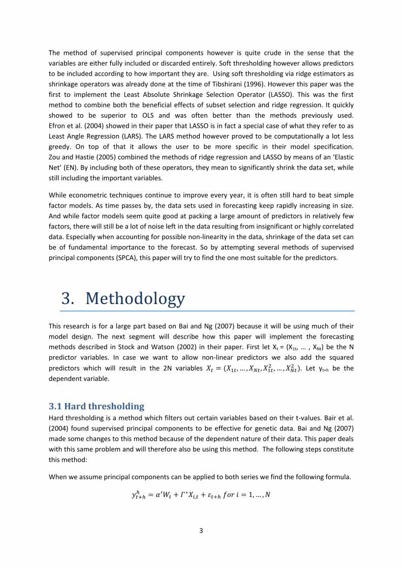
When we assume principal components can be applied to both series we find the following formula.

4

Here Wt contains a constant and lags of y. Alpha and Γ are least squares estimates. Van Dongen et al.

2013 found however that including lags did not improve the performance for personal income,

industrial production and non-agricultural employment, so the Wt will be left out. This results in an

alpha which solely estimates an intercept. After performing this regression we find the t-static ti for

each of the predictor variables. However this will not be done via the conventional way, since we

might be dealing with heteroskedasticity. Instead we will be using the heteroskedasticity and auto-

correlation consistent (HAC) standard errors as seen in Newey & West (1987). This allows us to

calculate the predictive power of Xit. We now include variable Xit in the set of targeted predictors if

|ti| exceeds a threshold significance level set by a significance level alpha. This allows us to apply

principal components, using the BIC to select the number of factors to include in our forecast. Our h

step ahead forecast will then be of the form

3.2 Soft thresholding There are several reasons why a hard thresholding method can be too crude. Because of the

discreteness of the decision rule, it can be very sensitive to small changes in the data. Also when

deciding on what variables to include, it does not take into account what information the other

predictors hold. So it is entirely possible that you will end up with very correlated predictors. Soft

thresholding on the other hand does not use this ‘all-or-nothing’ approach. Instead of setting

variables below the threshold to zero, soft thresholding methods merely attenuate them.

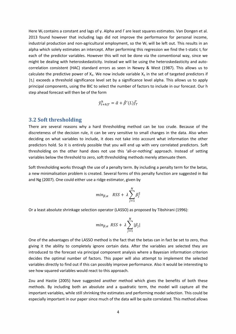
Soft thresholding works through the use of a penalty term. By including a penalty term for the betas,

a new minimalisation problem is created. Several forms of this penalty function are suggested in Bai

and Ng (2007). One could either use a ridge estimator, given by

∑

Or a least absolute shrinkage selection operator (LASSO) as proposed by Tibshirani (1996):

∑

One of the advantages of the LASSO method is the fact that the betas can in fact be set to zero, thus

giving it the ability to completely ignore certain data. After the variables are selected they are

introduced to the forecast via principal component analysis where a Bayesian information criterion

decides the optimal number of factors. This paper will also attempt to implement the selected

variables directly to find out if this can possibly improve performance. Also it would be interesting to

see how squared variables would react to this approach.

Zou and Hastie (2005) have suggested another method which gives the benefits of both these

methods. By including both an absolute and a quadratic term, the model will capture all the

important variables, while still shrinking the estimates and performing model selection. This could be

especially important in our paper since much of the data will be quite correlated. This method allows

5

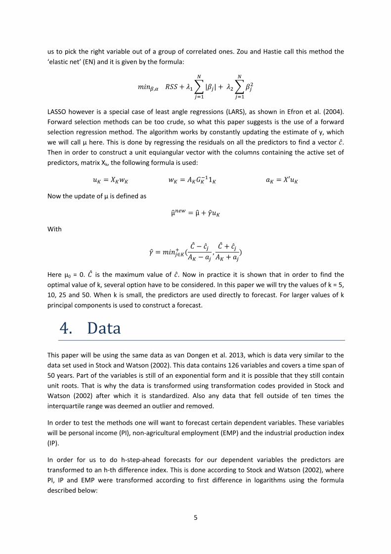
us to pick the right variable out of a group of correlated ones. Zou and Hastie call this method the

‘elastic net’ (EN) and it is given by the formula:

∑

∑

LASSO however is a special case of least angle regressions (LARS), as shown in Efron et al. (2004).

Forward selection methods can be too crude, so what this paper suggests is the use of a forward

selection regression method. The algorithm works by constantly updating the estimate of y, which

we will call µ here. This is done by regressing the residuals on all the predictors to find a vector .

Then in order to construct a unit equiangular vector with the columns containing the active set of

predictors, matrix Xk, the following formula is used:

Now the update of µ is defined as

With

Here 0 = 0. is the maximum value of . Now in practice it is shown that in order to find the

optimal value of k, several option have to be considered. In this paper we will try the values of k = 5,

10, 25 and 50. When k is small, the predictors are used directly to forecast. For larger values of k

principal components is used to construct a forecast.

4. Data

This paper will be using the same data as van Dongen et al. 2013, which is data very similar to the

data set used in Stock and Watson (2002). This data contains 126 variables and covers a time span of

50 years. Part of the variables is still of an exponential form and it is possible that they still contain

unit roots. That is why the data is transformed using transformation codes provided in Stock and

Watson (2002) after which it is standardized. Also any data that fell outside of ten times the

interquartile range was deemed an outlier and removed.

In order to test the methods one will want to forecast certain dependent variables. These variables

will be personal income (PI), non-agricultural employment (EMP) and the industrial production index

(IP).

In order for us to do h-step-ahead forecasts for our dependent variables the predictors are

transformed to an h-th difference index. This is done according to Stock and Watson (2002), where

PI, IP and EMP were transformed according to first difference in logarithms using the formula

described below:

6

(

)

In addition to this, the squared values of all variables were added to account for possible non-

linearity in the data. The end result was a data set containing 252 variables spanning a time period of

50 years.

5. Results

The in-sample period used will span the time from March 1960 until December 1989. This leaves us

with an out-of-sample period ranging from January 1990 until September 2009.

In order to compare the results, a benchmark had to be chosen. As is done in Bai & Ng (2007) an

AR(4) model was chosen. This is simple model, yet a tough benchmark to beat. In order to compare

the different methods to this benchmark the relative forecast mean squared error (RFMSE) was

calculated. This was done via the following formula:

5.1 Hard thresholding Table 1 contains the results of the three explained variables, personal income (PI), industrial

production (IP) and non-agricultural employment (EMP). For the AR(4) model we listed the actual

FMSE, since this model will play the part of benchmark. The other values indicate the RFMSE. So

here the AR(4) model would have an RFMSE of 1.00. For example the normal data set with a 5%

threshold has an RFMSE of 1.109, which means it has an FMSE of 110.9% that of the AR(4) model.

The values in this table include RFMSEs spanning four different thresholds of 1, 5, 10 and 20%. Also a

distinction is made between the normal data set, and the data set including the squared values of

the variables.

7

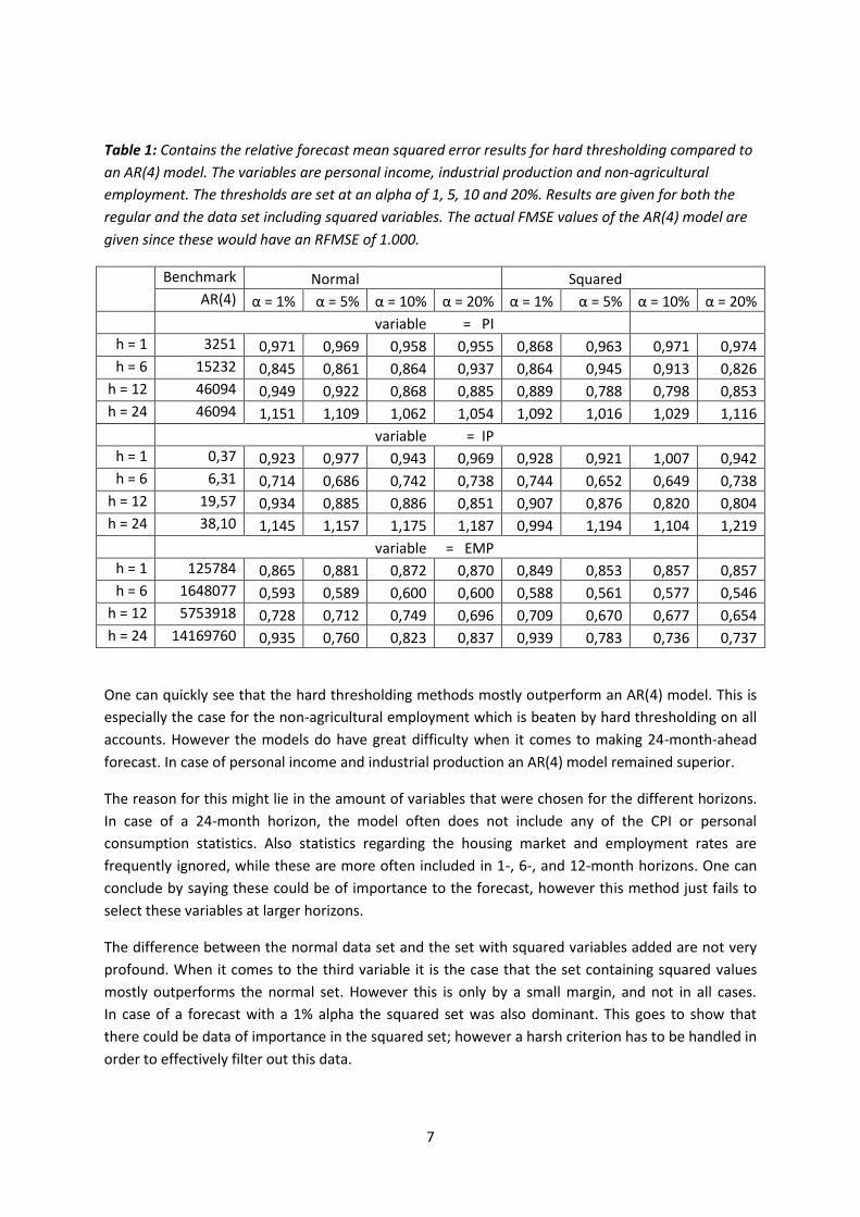
Table 1: Contains the relative forecast mean squared error results for hard thresholding compared to

an AR(4) model. The variables are personal income, industrial production and non-agricultural

employment. The thresholds are set at an alpha of 1, 5, 10 and 20%. Results are given for both the

regular and the data set including squared variables. The actual FMSE values of the AR(4) model are

given since these would have an RFMSE of 1.000.

Benchmark Normal Squared

AR(4) α = 1% α = 5% α = 10% α = 20% α = 1% α = 5% α = 10% α = 20%

variable = PI

h = 1 3251 0,971 0,969 0,958 0,955 0,868 0,963 0,971 0,974

h = 6 15232 0,845 0,861 0,864 0,937 0,864 0,945 0,913 0,826

h = 12 46094 0,949 0,922 0,868 0,885 0,889 0,788 0,798 0,853

h = 24 46094 1,151 1,109 1,062 1,054 1,092 1,016 1,029 1,116

variable = IP

h = 1 0,37 0,923 0,977 0,943 0,969 0,928 0,921 1,007 0,942

h = 6 6,31 0,714 0,686 0,742 0,738 0,744 0,652 0,649 0,738

h = 12 19,57 0,934 0,885 0,886 0,851 0,907 0,876 0,820 0,804

h = 24 38,10 1,145 1,157 1,175 1,187 0,994 1,194 1,104 1,219

variable = EMP

h = 1 125784 0,865 0,881 0,872 0,870 0,849 0,853 0,857 0,857

h = 6 1648077 0,593 0,589 0,600 0,600 0,588 0,561 0,577 0,546

h = 12 5753918 0,728 0,712 0,749 0,696 0,709 0,670 0,677 0,654

h = 24 14169760 0,935 0,760 0,823 0,837 0,939 0,783 0,736 0,737

One can quickly see that the hard thresholding methods mostly outperform an AR(4) model. This is

especially the case for the non-agricultural employment which is beaten by hard thresholding on all

accounts. However the models do have great difficulty when it comes to making 24-month-ahead

forecast. In case of personal income and industrial production an AR(4) model remained superior.

The reason for this might lie in the amount of variables that were chosen for the different horizons.

In case of a 24-month horizon, the model often does not include any of the CPI or personal

consumption statistics. Also statistics regarding the housing market and employment rates are

frequently ignored, while these are more often included in 1-, 6-, and 12-month horizons. One can

conclude by saying these could be of importance to the forecast, however this method just fails to

select these variables at larger horizons.

The difference between the normal data set and the set with squared variables added are not very

profound. When it comes to the third variable it is the case that the set containing squared values

mostly outperforms the normal set. However this is only by a small margin, and not in all cases.

In case of a forecast with a 1% alpha the squared set was also dominant. This goes to show that

there could be data of importance in the squared set; however a harsh criterion has to be handled in

order to effectively filter out this data.

8

5.2 LASSO In table 2 we find the results of the LASSO method, as suggested in Tibshirani (1996). These results

include both the selected variables being used directly in the forecast, and the results of these

variables being used in a forecast via principal component analysis.

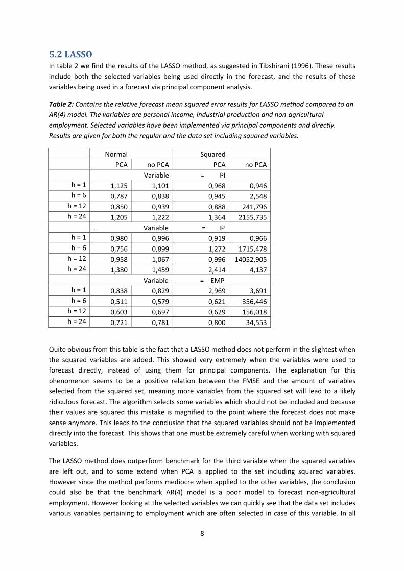
Table 2: Contains the relative forecast mean squared error results for LASSO method compared to an

AR(4) model. The variables are personal income, industrial production and non-agricultural

employment. Selected variables have been implemented via principal components and directly.

Results are given for both the regular and the data set including squared variables.

Normal Squared

PCA no PCA PCA no PCA

Variable = PI

h = 1 1,125 1,101 0,968 0,946

h = 6 0,787 0,838 0,945 2,548

h = 12 0,850 0,939 0,888 241,796

h = 24 1,205 1,222 1,364 2155,735

. Variable = IP h = 1 0,980 0,996 0,919 0,966

h = 6 0,756 0,899 1,272 1715,478

h = 12 0,958 1,067 0,996 14052,905

h = 24 1,380 1,459 2,414 4,137

Variable = EMP

h = 1 0,838 0,829 2,969 3,691

h = 6 0,511 0,579 0,621 356,446

h = 12 0,603 0,697 0,629 156,018

h = 24 0,721 0,781 0,800 34,553

Quite obvious from this table is the fact that a LASSO method does not perform in the slightest when

the squared variables are added. This showed very extremely when the variables were used to

forecast directly, instead of using them for principal components. The explanation for this

phenomenon seems to be a positive relation between the FMSE and the amount of variables

selected from the squared set, meaning more variables from the squared set will lead to a likely

ridiculous forecast. The algorithm selects some variables which should not be included and because

their values are squared this mistake is magnified to the point where the forecast does not make

sense anymore. This leads to the conclusion that the squared variables should not be implemented

directly into the forecast. This shows that one must be extremely careful when working with squared

variables.

The LASSO method does outperform benchmark for the third variable when the squared variables

are left out, and to some extend when PCA is applied to the set including squared variables.

However since the method performs mediocre when applied to the other variables, the conclusion

could also be that the benchmark AR(4) model is a poor model to forecast non-agricultural

employment. However looking at the selected variables we can quickly see that the data set includes

various variables pertaining to employment which are often selected in case of this variable. In all

9

three of the variables the variables relating to bond yields and FF-spreads were often chosen. Also

the variable pertaining to the money total classified as M2 was popular.

5.3 Elastic Net Displayed below in table 3 are the results of the ‘Elastic Net’ procedure as suggested in Zou and

Hastie (2005). It contains data for three different values of lambda, being 0.5, 0.25 and 0.10. The

variables have been implemented via principal components. The RFMSEs are given for both the

normal set, and the set containing the squared values of the data.

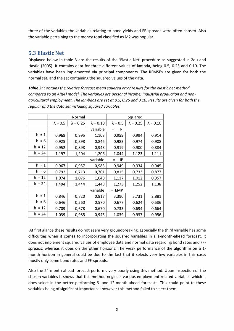
Table 3: Contains the relative forecast mean squared error results for the elastic net method

compared to an AR(4) model. The variables are personal income, industrial production and non-

agricultural employment. The lambdas are set at 0.5, 0.25 and 0.10. Results are given for both the

regular and the data set including squared variables.

Normal Squared

λ = 0.5 λ = 0.25 λ = 0.10 λ = 0.5 λ = 0.25 λ = 0.10

variable = PI

h = 1 0,968 0,995 1,103 0,959 0,994 0,914

h = 6 0,925 0,898 0,845 0,983 0,974 0,908

h = 12 0,952 0,898 0,943 0,919 0,900 0,884

h = 24 1,197 1,204 1,206 1,044 1,123 1,111

variable = IP

h = 1 0,967 0,957 0,983 0,949 0,934 0,945

h = 6 0,792 0,713 0,701 0,815 0,733 0,877

h = 12 1,074 1,076 1,048 1,117 1,012 0,957

h = 24 1,494 1,444 1,448 1,273 1,252 1,138

variable = EMP

h = 1 0,846 0,820 0,817 3,390 3,731 2,881

h = 6 0,646 0,560 0,570 0,677 0,624 0,586

h = 12 0,709 0,678 0,670 0,733 0,694 0,664

h = 24 1,039 0,985 0,945 1,039 0,937 0,956

At first glance these results do not seem very groundbreaking. Especially the third variable has some

difficulties when it comes to incorporating the squared variables in a 1-month-ahead forecast. It

does not implement squared values of employee data and normal data regarding bond rates and FF-

spreads, whereas it does on the other horizons. The weak performance of the algorithm on a 1-

month horizon in general could be due to the fact that it selects very few variables in this case,

mostly only some bond rates and FF-spreads.

Also the 24-month-ahead forecast performs very poorly using this method. Upon inspection of the

chosen variables it shows that this method neglects various employment related variables which it

does select in the better performing 6- and 12-month-ahead forecasts. This could point to these

variables being of significant importance; however this method failed to select them.

10

The lambda giving the best results is varying. These specific lambdas were chosen because lambdas

higher than these values proved to give bad results. Smaller values also gave bad results. A grid

search proved to be too computationally exhaustive. These lambdas give a reasonable selection of

values within a range of feasible results.

When comparing the results of the normal data set and the set including squared values, it is

apparent that the normal data set performs superior on almost all accounts. Especially the 1-month

horizon for the third variable gives results much worse when the squared variables are included. An

explanation for this could be that some squared variables were selected at some point in time

ruining the entire FMSE. This goes to show that when working with squared variables, one has to be

extremely careful. Including squared variables has not been giving inferior results for every method

used in this paper. This method seems unequipped to handle this extra information resulting in poor

results.

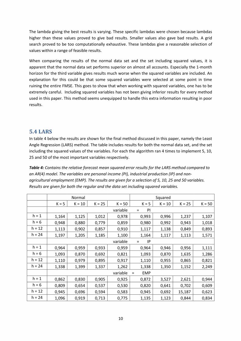
5.4 LARS In table 4 below the results are shown for the final method discussed in this paper, namely the Least

Angle Regression (LARS) method. The table includes results for both the normal data set, and the set

including the squared values of the variables. For each the algorithm ran 4 times to implement 5, 10,

25 and 50 of the most important variables respectively.

Table 4: Contains the relative forecast mean squared error results for the LARS method compared to

an AR(4) model. The variables are personal income (PI), industrial production (IP) and non-

agricultural employment (EMP). The results are given for a selection of 5, 10, 25 and 50 variables.

Results are given for both the regular and the data set including squared variables.

Normal Squared

K = 5 K = 10 K = 25 K = 50 K = 5 K = 10 K = 25 K = 50

variable = PI

h = 1 1,164 1,125 1,012 0,978 0,993 0,996 1,237 1,107

h = 6 0,948 0,880 0,779 0,859 0,980 0,992 0,943 1,018

h = 12 1,113 0,902 0,857 0,910 1,117 1,138 0,849 0,893

h = 24 1,197 1,205 1,185 1,100 1,164 1,117 1,113 1,571

variable = IP

h = 1 0,964 0,959 0,933 0,959 0,964 0,946 0,956 1,111

h = 6 1,093 0,870 0,692 0,821 1,093 0,870 1,635 1,286

h = 12 1,110 0,979 0,895 0,917 1,110 0,955 0,865 0,821

h = 24 1,338 1,399 1,337 1,262 1,338 1,350 1,152 2,249

variable = EMP

h = 1 0,862 0,830 0,905 0,925 0,872 3,527 2,621 0,944

h = 6 0,809 0,654 0,537 0,530 0,820 0,641 0,702 0,609

h = 12 0,945 0,696 0,594 0,583 0,945 0,692 15,187 0,623

h = 24 1,096 0,919 0,713 0,775 1,135 1,123 0,844 0,834

11

Also this method has the greatest of problems outperforming an AR(4) model. The outlier in

forecasting non-agricultural employment for the third variable including squared variables is hard to

explain. One instance of bad variable selection could potentially be fatal to the FMSE, which is likely

what happened here.

As well as the other methods, the LARS method especially has problems beating the AR(4) model on

a 24-month horizon. The AR(4) model is a strong benchmark for the 24-month horizon, but this is

disappointing nonetheless. As we’ve seen in previous methods, also this method focuses heavily on

the employment market (regardless of the dependent variable) and several FF-spreads. Especially

when fewer variables are available, the selection algorithm does not seem very dynamic.

The normal set dominates the larger set on most occasions. This shows that the incorporation of

squared valuables is not a task that every method is capable of handling. Furthermore it could point

to the fact that adding the squared values of the variables is not relevant given our data.

6. Conclusion

When looking at the different models, it quickly becomes apparent that it is very hard to beat a

simple benchmark model containing 4 autoregressive terms. Only in case of non-agricultural

employment where the methods used consistently better than an AR(4) model. This is in part

however due to a poor performance of the benchmark model in this case. Also given the fact that

this model performs very strongly on a 24-month horizon made for a tough challenge.

However, on various forecast horizons the different methods often prove a lot better than the AR(4)

model. Especially on 6 and 12 month horizons the benchmark was beaten most of the time.

Consistency is key here however, as a good model should work for a variety of horizons and

variables.

Variable selection proves a difficult trial throughout each of the methods used. For each variable and

horizon one can see a different subset of predictors chosen, which leads to the question of whether

or not the algorithm was right to select the variables it did. Since each of the methods incorporates

all the data into the subset selecting algorithm there is not much room for dynamics in the selected

variables. It would be interesting to see how such a model would react when only more recent data

was used to choose the predictors. In this way any structural breaks could be much better captured.

For most methods adding squared values of the data did not yield any improvement. Only the hard

thresholding method was able to make use of this data with some consistency. Though whether a

harsh or a more forgiving threshold was best is hard to say. A harsh threshold seems wisest since

this reduces the risk of introducing variables which harm the forecast. This also shows from the

results where these values proved the most consistent.

Through the use of the soft thresholding methods, incorporating squared values of the data cannot

be justified. Outliers in the results and overall poor performance make it unnecessarily risky. The

volatility of this data has proven itself quite dangerous. More extensive research or specified

12

methods have to be applied to make sure that only the right variables get selected. Again to solve

this problem a moving window would seem an interesting research opportunity, since this would

allow for more dynamic variable selection.

Another interesting venture could be the combination of several forecasts. By combining forecasts

with different thresholds the results can be hedged against potential mistakes in the data selection

process. Especially when dealing with squared variables this can be of importance because a mistake

is quickly made.

7. References

J. Bai, S. Ng, 2007, Forecasting economic time series using targeted predictors. Journal of

Econometrics, 146(2):304-317

Bair, E., Hastie, T., Paul, D. and Tibshirani, R. 2006, Prediction by Supervised Principal Components, Journal of the American Statistical Association 101:473, 119–137. Boivin, J. and Ng, S. 2006, Are More Data Always Better for Factor Analysis, Journal of Econometrics 132, 169–194. Van Dongen, T.J., Klaassens, P., Kop, J.S. and Tijssen, L.S. 2013 Averaging Forecasts Across Number of Factors Donoho, D. and Johnstone, I. 1994, Ideal Spatial Adaptiationby Wavelet Shrinkage, Biometrika 81, 425–455. Efron, B., Hastie, T., Johnstone, I. and Tibshirani, R. 2004, Least Angle Regression, Annals of Statistics

32:2, 407–499.

Newey, Whitney K. West, Kenneth D. 1987, A Simple, Positive Semi-definite, Heteroskedasticity and

Autocorrelation Consistent Covariance Matrix. Econometrica 55 (3): 703–708.

Roberts,S. Martin, M. A. 2006, Using Supervised Principal Component Analysis to Assess Multiple

Pollutant Effects, Environ Health Perspect, 114:1877-1882

Stock, J. H. and Watson, M. W. 2002, Forecasting Using Principal Components from a Large Number

of Predictors, Journal of the American Statistical Association 97, 1167–1179.

Tibshirani, R. 1996, Regression Shrinkage and Selection via the Lasso, Journal of Royal Statistical

Society Series B 58:1, 267–288.

Zou, H. and Hastie, T. 2005, Regularization and Variable Selection via the Elastic Net, Journal of Royal

Statistical Society, Series B 67:2, 301–320.

8. Appendix

13

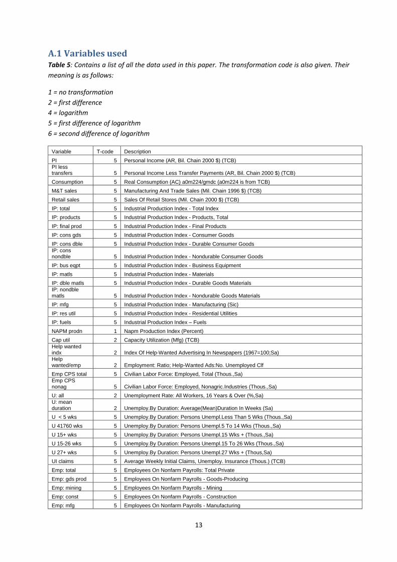
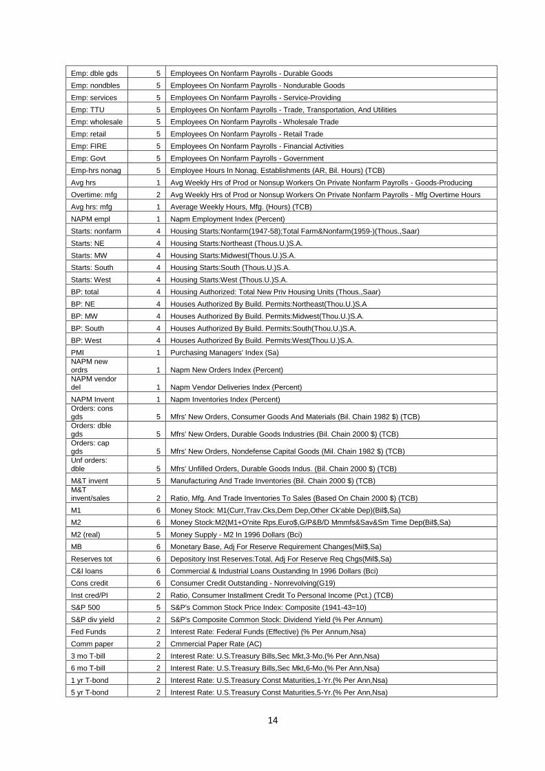
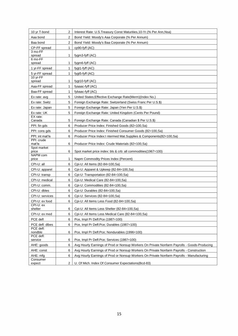
A.1 Variables used Table 5: Contains a list of all the data used in this paper. The transformation code is also given. Their

meaning is as follows:

1 = no transformation

2 = first difference

4 = logarithm

5 = first difference of logarithm

6 = second difference of logarithm

Variable T-code Description

PI 5 Personal Income (AR, Bil. Chain 2000 $) (TCB)

PI less transfers 5 Personal Income Less Transfer Payments (AR, Bil. Chain 2000 $) (TCB)

Consumption 5 Real Consumption (AC) a0m224/gmdc (a0m224 is from TCB)

M&T sales 5 Manufacturing And Trade Sales (Mil. Chain 1996 $) (TCB)

Retail sales 5 Sales Of Retail Stores (Mil. Chain 2000 $) (TCB)

IP: total 5 Industrial Production Index - Total Index

IP: products 5 Industrial Production Index - Products, Total

IP: final prod 5 Industrial Production Index - Final Products

IP: cons gds 5 Industrial Production Index - Consumer Goods

IP: cons dble 5 Industrial Production Index - Durable Consumer Goods

IP: cons nondble 5 Industrial Production Index - Nondurable Consumer Goods

IP: bus eqpt 5 Industrial Production Index - Business Equipment

IP: matls 5 Industrial Production Index - Materials

IP: dble matls 5 Industrial Production Index - Durable Goods Materials

IP: nondble matls 5 Industrial Production Index - Nondurable Goods Materials

IP: mfg 5 Industrial Production Index - Manufacturing (Sic)

IP: res util 5 Industrial Production Index - Residential Utilities

IP: fuels 5 Industrial Production Index – Fuels

NAPM prodn 1 Napm Production Index (Percent)

Cap util 2 Capacity Utilization (Mfg) (TCB)

Help wanted indx 2 Index Of Help-Wanted Advertising In Newspapers (1967=100;Sa)

Help wanted/emp 2 Employment: Ratio; Help-Wanted Ads:No. Unemployed Clf

Emp CPS total 5 Civilian Labor Force: Employed, Total (Thous.,Sa)

Emp CPS nonag 5 Civilian Labor Force: Employed, Nonagric.Industries (Thous.,Sa)

U: all 2 Unemployment Rate: All Workers, 16 Years & Over (%,Sa)

U: mean duration 2 Unemploy.By Duration: Average(Mean)Duration In Weeks (Sa)

U < 5 wks 5 Unemploy.By Duration: Persons Unempl.Less Than 5 Wks (Thous.,Sa)

U 41760 wks 5 Unemploy.By Duration: Persons Unempl.5 To 14 Wks (Thous.,Sa)

U 15+ wks 5 Unemploy.By Duration: Persons Unempl.15 Wks + (Thous.,Sa)

U 15-26 wks 5 Unemploy.By Duration: Persons Unempl.15 To 26 Wks (Thous.,Sa)

U 27+ wks 5 Unemploy.By Duration: Persons Unempl.27 Wks + (Thous,Sa)

UI claims 5 Average Weekly Initial Claims, Unemploy. Insurance (Thous.) (TCB)

Emp: total 5 Employees On Nonfarm Payrolls: Total Private

Emp: gds prod 5 Employees On Nonfarm Payrolls - Goods-Producing

Emp: mining 5 Employees On Nonfarm Payrolls - Mining

Emp: const 5 Employees On Nonfarm Payrolls - Construction

Emp: mfg 5 Employees On Nonfarm Payrolls - Manufacturing

14

Emp: dble gds 5 Employees On Nonfarm Payrolls - Durable Goods

Emp: nondbles 5 Employees On Nonfarm Payrolls - Nondurable Goods

Emp: services 5 Employees On Nonfarm Payrolls - Service-Providing

Emp: TTU 5 Employees On Nonfarm Payrolls - Trade, Transportation, And Utilities

Emp: wholesale 5 Employees On Nonfarm Payrolls - Wholesale Trade

Emp: retail 5 Employees On Nonfarm Payrolls - Retail Trade

Emp: FIRE 5 Employees On Nonfarm Payrolls - Financial Activities

Emp: Govt 5 Employees On Nonfarm Payrolls - Government

Emp-hrs nonag 5 Employee Hours In Nonag. Establishments (AR, Bil. Hours) (TCB)

Avg hrs 1 Avg Weekly Hrs of Prod or Nonsup Workers On Private Nonfarm Payrolls - Goods-Producing

Overtime: mfg 2 Avg Weekly Hrs of Prod or Nonsup Workers On Private Nonfarm Payrolls - Mfg Overtime Hours

Avg hrs: mfg 1 Average Weekly Hours, Mfg. (Hours) (TCB)

NAPM empl 1 Napm Employment Index (Percent)

Starts: nonfarm 4 Housing Starts:Nonfarm(1947-58);Total Farm&Nonfarm(1959-)(Thous.,Saar)

Starts: NE 4 Housing Starts:Northeast (Thous.U.)S.A.

Starts: MW 4 Housing Starts:Midwest(Thous.U.)S.A.

Starts: South 4 Housing Starts:South (Thous.U.)S.A.

Starts: West 4 Housing Starts:West (Thous.U.)S.A.

BP: total 4 Housing Authorized: Total New Priv Housing Units (Thous.,Saar)

BP: NE 4 Houses Authorized By Build. Permits:Northeast(Thou.U.)S.A

BP: MW 4 Houses Authorized By Build. Permits:Midwest(Thou.U.)S.A.

BP: South 4 Houses Authorized By Build. Permits:South(Thou.U.)S.A.

BP: West 4 Houses Authorized By Build. Permits:West(Thou.U.)S.A.

PMI 1 Purchasing Managers' Index (Sa)

NAPM new ordrs 1 Napm New Orders Index (Percent)

NAPM vendor del 1 Napm Vendor Deliveries Index (Percent)

NAPM Invent 1 Napm Inventories Index (Percent)

Orders: cons gds 5 Mfrs' New Orders, Consumer Goods And Materials (Bil. Chain 1982 $) (TCB)

Orders: dble gds 5 Mfrs' New Orders, Durable Goods Industries (Bil. Chain 2000 $) (TCB)

Orders: cap gds 5 Mfrs' New Orders, Nondefense Capital Goods (Mil. Chain 1982 $) (TCB)

Unf orders: dble 5 Mfrs' Unfilled Orders, Durable Goods Indus. (Bil. Chain 2000 $) (TCB)

M&T invent 5 Manufacturing And Trade Inventories (Bil. Chain 2000 $) (TCB)

M&T invent/sales 2 Ratio, Mfg. And Trade Inventories To Sales (Based On Chain 2000 $) (TCB)

M1 6 Money Stock: M1(Curr,Trav.Cks,Dem Dep,Other Ck'able Dep)(Bil$,Sa)

M2 6 Money Stock:M2(M1+O'nite Rps,Euro$,G/P&B/D Mmmfs&Sav&Sm Time Dep(Bil$,Sa)

M2 (real) 5 Money Supply - M2 In 1996 Dollars (Bci)

MB 6 Monetary Base, Adj For Reserve Requirement Changes(Mil$,Sa)

Reserves tot 6 Depository Inst Reserves:Total, Adj For Reserve Req Chgs(Mil$,Sa)

C&I loans 6 Commercial & Industrial Loans Oustanding In 1996 Dollars (Bci)

Cons credit 6 Consumer Credit Outstanding - Nonrevolving(G19)

Inst cred/PI 2 Ratio, Consumer Installment Credit To Personal Income (Pct.) (TCB)

S&P 500 5 S&P's Common Stock Price Index: Composite (1941-43=10)

S&P div yield 2 S&P's Composite Common Stock: Dividend Yield (% Per Annum)

Fed Funds 2 Interest Rate: Federal Funds (Effective) (% Per Annum,Nsa)

Comm paper 2 Cmmercial Paper Rate (AC)

3 mo T-bill 2 Interest Rate: U.S.Treasury Bills,Sec Mkt,3-Mo.(% Per Ann,Nsa)

6 mo T-bill 2 Interest Rate: U.S.Treasury Bills,Sec Mkt,6-Mo.(% Per Ann,Nsa)

1 yr T-bond 2 Interest Rate: U.S.Treasury Const Maturities,1-Yr.(% Per Ann,Nsa)


15


Aaa bond 2 Bond Yield: Moody's Aaa Corporate (% Per Annum)

Baa bond 2 Bond Yield: Moody's Baa Corporate (% Per Annum)

CP-FF spread 1 cp90-fyff (AC)

3 mo-FF spread 1 fygm3-fyff (AC)

6 mo-FF spread 1 fygm6-fyff (AC)

1 yr-FF spread 1 fygt1-fyff (AC)



Aaa-FF spread 1 fyaaac-fyff (AC)

Baa-FF spread 1 fybaac-fyff (AC)

Ex rate: avg 5 United States;Effective Exchange Rate(Merm)(Index No.)

Ex rate: Switz 5 Foreign Exchange Rate: Switzerland (Swiss Franc Per U.S.$)

Ex rate: Japan 5 Foreign Exchange Rate: Japan (Yen Per U.S.$)

Ex rate: UK 5 Foreign Exchange Rate: United Kingdom (Cents Per Pound)

EX rate: Canada 5 Foreign Exchange Rate: Canada (Canadian $ Per U.S.$)

PPI: fin gds 6 Producer Price Index: Finished Goods (82=100,Sa)

PPI: cons gds 6 Producer Price Index: Finished Consumer Goods (82=100,Sa)

PPI: int mat’ls 6 Producer Price Index:I ntermed Mat.Supplies & Components(82=100,Sa)

PPI: crude mat’ls 6 Producer Price Index: Crude Materials (82=100,Sa)

Spot market price 6 Spot market price index: bls & crb: all commodities(1967=100)

NAPM com price 1 Napm Commodity Prices Index (Percent)

CPI-U: all 6 Cpi-U: All Items (82-84=100,Sa)

CPI-U: apparel 6 Cpi-U: Apparel & Upkeep (82-84=100,Sa)

CPI-U: transp 6 Cpi-U: Transportation (82-84=100,Sa)

CPI-U: medical 6 Cpi-U: Medical Care (82-84=100,Sa)

CPI-U: comm. 6 Cpi-U: Commodities (82-84=100,Sa)

CPI-U: dbles 6 Cpi-U: Durables (82-84=100,Sa)

CPI-U: services 6 Cpi-U: Services (82-84=100,Sa)

CPI-U: ex food 6 Cpi-U: All Items Less Food (82-84=100,Sa)

CPI-U: ex shelter 6 Cpi-U: All Items Less Shelter (82-84=100,Sa)

CPI-U: ex med 6 Cpi-U: All Items Less Medical Care (82-84=100,Sa)

PCE defl 6 Pce, Impl Pr Defl:Pce (1987=100)

PCE defl: dlbes 6 Pce, Impl Pr Defl:Pce; Durables (1987=100)

PCE defl: nondble 6 Pce, Impl Pr Defl:Pce; Nondurables (1996=100)

PCE defl: service 6 Pce, Impl Pr Defl:Pce; Services (1987=100)

AHE: goods 6 Avg Hourly Earnings of Prod or Nonsup Workers On Private Nonfarm Payrolls - Goods-Producing

AHE: const 6 Avg Hourly Earnings of Prod or Nonsup Workers On Private Nonfarm Payrolls - Construction

AHE: mfg 6 Avg Hourly Earnings of Prod or Nonsup Workers On Private Nonfarm Payrolls - Manufacturing

Consumer expect 2 U. Of Mich. Index Of Consumer Expectations(Bcd-83)

16

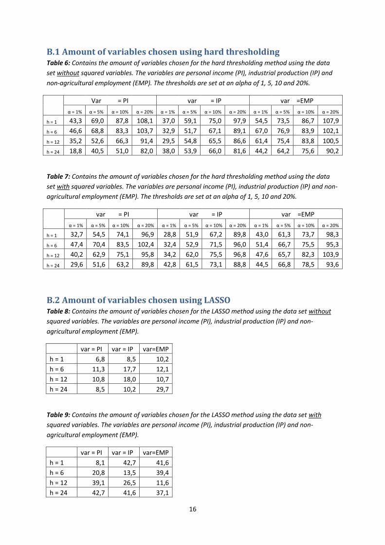
B.1 Amount of variables chosen using hard thresholding Table 6: Contains the amount of variables chosen for the hard thresholding method using the data

set without squared variables. The variables are personal income (PI), industrial production (IP) and

non-agricultural employment (EMP). The thresholds are set at an alpha of 1, 5, 10 and 20%.

Var = PI var = IP var =EMP

α = 1% α = 5% α = 10% α = 20% α = 1% α = 5% α = 10% α = 20% α = 1% α = 5% α = 10% α = 20%

h = 1 43,3 69,0 87,8 108,1 37,0 59,1 75,0 97,9 54,5 73,5 86,7 107,9

h = 6 46,6 68,8 83,3 103,7 32,9 51,7 67,1 89,1 67,0 76,9 83,9 102,1

h = 12 35,2 52,6 66,3 91,4 29,5 54,8 65,5 86,6 61,4 75,4 83,8 100,5

h = 24 18,8 40,5 51,0 82,0 38,0 53,9 66,0 81,6 44,2 64,2 75,6 90,2

Table 7: Contains the amount of variables chosen for the hard thresholding method using the data

set with squared variables. The variables are personal income (PI), industrial production (IP) and non-

agricultural employment (EMP). The thresholds are set at an alpha of 1, 5, 10 and 20%.

var = PI var = IP var =EMP

α = 1% α = 5% α = 10% α = 20% α = 1% α = 5% α = 10% α = 20% α = 1% α = 5% α = 10% α = 20%

h = 1 32,7 54,5 74,1 96,9 28,8 51,9 67,2 89,8 43,0 61,3 73,7 98,3

h = 6 47,4 70,4 83,5 102,4 32,4 52,9 71,5 96,0 51,4 66,7 75,5 95,3

h = 12 40,2 62,9 75,1 95,8 34,2 62,0 75,5 96,8 47,6 65,7 82,3 103,9

h = 24 29,6 51,6 63,2 89,8 42,8 61,5 73,1 88,8 44,5 66,8 78,5 93,6

B.2 Amount of variables chosen using LASSO Table 8: Contains the amount of variables chosen for the LASSO method using the data set without

squared variables. The variables are personal income (PI), industrial production (IP) and non-

agricultural employment (EMP).

var = PI var = IP var=EMP

h = 1 6,8 8,5 10,2

h = 6 11,3 17,7 12,1

h = 12 10,8 18,0 10,7

h = 24 8,5 10,2 29,7

Table 9: Contains the amount of variables chosen for the LASSO method using the data set with


agricultural employment (EMP).


h = 1 8,1 42,7 41,6

h = 6 20,8 13,5 39,4

h = 12 39,1 26,5 11,6

h = 24 42,7 41,6 37,1

17

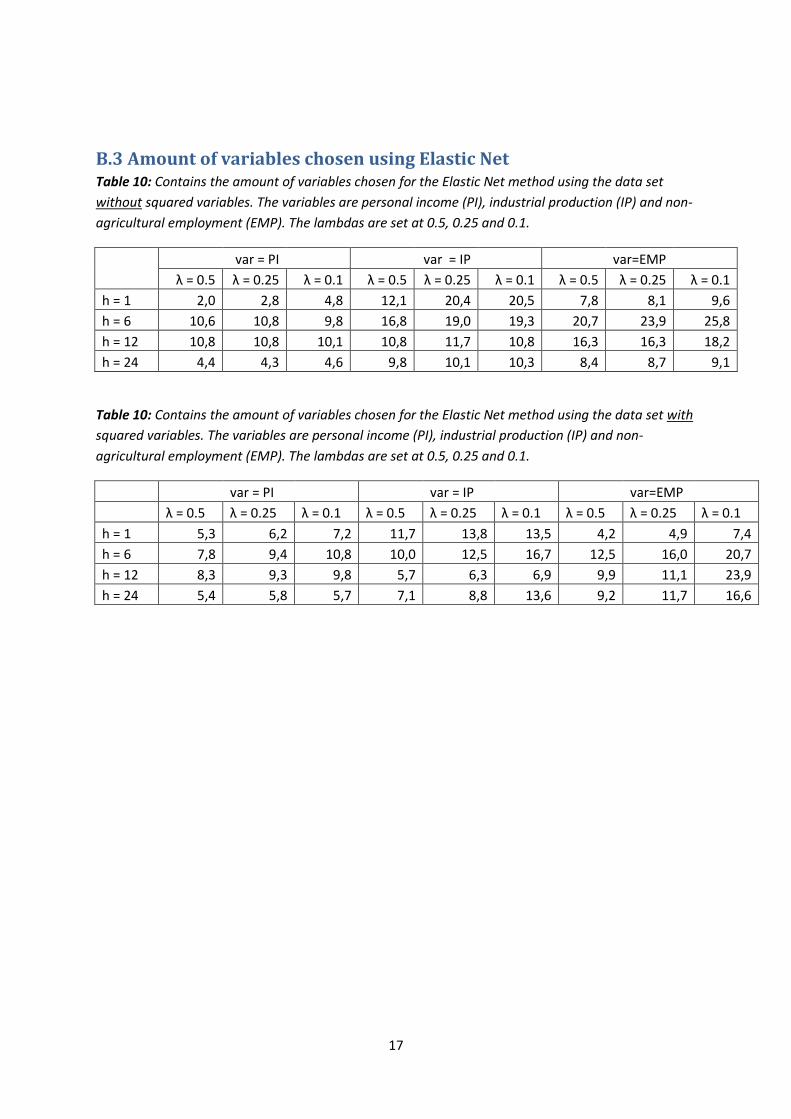
B.3 Amount of variables chosen using Elastic Net Table 10: Contains the amount of variables chosen for the Elastic Net method using the data set

without squared variables. The variables are personal income (PI), industrial production (IP) and non-

agricultural employment (EMP). The lambdas are set at 0.5, 0.25 and 0.1.


λ = 0.5 λ = 0.25 λ = 0.1 λ = 0.5 λ = 0.25 λ = 0.1 λ = 0.5 λ = 0.25 λ = 0.1

h = 1 2,0 2,8 4,8 12,1 20,4 20,5 7,8 8,1 9,6

h = 6 10,6 10,8 9,8 16,8 19,0 19,3 20,7 23,9 25,8

h = 12 10,8 10,8 10,1 10,8 11,7 10,8 16,3 16,3 18,2

h = 24 4,4 4,3 4,6 9,8 10,1 10,3 8,4 8,7 9,1

Table 10: Contains the amount of variables chosen for the Elastic Net method using the data set with


agricultural employment (EMP). The lambdas are set at 0.5, 0.25 and 0.1.


λ = 0.5 λ = 0.25 λ = 0.1 λ = 0.5 λ = 0.25 λ = 0.1 λ = 0.5 λ = 0.25 λ = 0.1

h = 1 5,3 6,2 7,2 11,7 13,8 13,5 4,2 4,9 7,4

h = 6 7,8 9,4 10,8 10,0 12,5 16,7 12,5 16,0 20,7

h = 12 8,3 9,3 9,8 5,7 6,3 6,9 9,9 11,1 23,9

h = 24 5,4 5,8 5,7 7,1 8,8 13,6 9,2 11,7 16,6

Documents

Predictor Selection in Forecasting Macro-Economic Variables