Embed Size (px)
Citation preview
Forecasting Stock Market Returns:
The Sum of the Parts is More than the Whole∗
Miguel A. Ferreira† Pedro Santa-Clara‡
This version: July 2010
Abstract
We propose forecasting separately the three components of stock market returns: the
dividend-price ratio, earnings growth, and price-earnings ratio growth – the sum-of-
the-parts (SOP) method. Our method exploits the different time-series persistence of
the components and obtains out-of-sample R-squares (compared to the historical mean)
of more than 1.3% with monthly data and 13.4% with yearly data. This compares
with typically negative R-squares obtained in a similar experiment with predictive
regressions. The performance of the SOP method comes mainly from the dividend-
price ratio and earnings growth components and the robustness of the method is due
to its low estimation error. An investor who timed the market using our method would
have had a Sharpe ratio gain of 0.3.
∗We thank an anonymous referee, Michael Brandt, Jules van Binsbergen, John Campbell, John Cochrane,Amit Goyal, Lubos Pastor, Bill Schwert (the editor), Ivo Welch, Motohiro Yogo, and Jialin Yu; seminar
participants at Barclays Global Investors, Goethe Universität Frankfurt, Hong Kong University of Science
and Technology Finance Symposium, Manchester Business School, Norwegian School of Management - BI,
and University of Piraeus; and participants at the 2009 European Finance Association Conference, 2010
American Finance Association Conference, and CSEF-IGIER Symposium on Economics and Institutions for
helpful comments. We are particularly grateful to Carolina Almeida, Filipe Lacerda, and Tymur Gabunya
for outstanding research assistance.†Universidade Nova de Lisboa - Faculdade de Economia and European Corporate Governance
Institute, Campus de Campolide, 1099-032 Lisboa, Portugal. Phone +351-21-3801600, E-mail:
[email protected].‡Millennium Chair in Finance. Universidade Nova de Lisboa - Faculdade de Economia and NBER,
Campus de Campolide, 1099-032 Lisboa, Portugal. Phone +351-21-3801600. E-mail: [email protected].

1. Introduction
There is a long literature on forecasting stock market returns using price multiples, macro-
economic variables, corporate actions, and measures of risk.1 These studies find evidence
in favor of return predictability in sample. However, a number of authors question these
findings on the grounds that the persistence of the forecasting variables and the correlation
of their innovations with returns might bias the regression coefficients and affect t-statistics;
see Nelson and Kim (1993), Cavanagh, Elliott, and Stock (1995), Stambaugh (1999), and
Lewellen (2004). A further problem is the possibility of data mining illustrated by a long
list of spurious predictive variables that regularly show up in the press, including hemlines,
football results, and butter production in Bangladesh; see Foster, Smith, and Whaley (1997),
and Ferson, Sarkissian, and Simin (2003). The predictability of stock market returns thus
remains an open question.
In important recent research, Goyal and Welch (2008) examine the out-of-sample perfor-
mance of a long list of predictors. They compare forecasts of returns at time + 1 from a
predictive regression estimated using data up to time with forecasts based on the historical
mean in the same period. They find that the historical mean actually has better out-of-
sample performance than the traditional predictive regressions. Goyal and Welch (2008)
conclude that “these models would not have helped an investor with access only to avail-
able information to profitably time the market” (p. 1455); see also Bossaerts and Hillion
(1999). While Inoue and Kilian (2004) and Cochrane (2008) argue that this is not evidence
against predictability per se but only evidence of the difficulty in exploiting predictability
1Researchers who use the dividend yield include Dow (1920), Campbell (1987), Fama and French (1988),
Hodrick (1992), Campbell and Yogo (2006), Ang and Bekaert (2007), Cochrane (2008), and Binsbergen and
Koijen (2010). The earnings-price ratio is used by Campbell and Shiller (1988) and Lamont (1998). The
book-to-market ratio is used by Kothari and Shanken (1997) and Pontiff and Schall (1998). The short-term
interest rate is used by Fama and Schwert (1977), Campbell (1987), Breen, Glosten, and Jagannathan (1989),
and Ang and Bekaert (2007). Inflation is used by Nelson (1976), Fama and Schwert (1977), Ritter and Warr
(2002), and Campbell and Vuolteenaho (2004). The term and default yield spreads are used by Campbell
(1987) and Fama and French (1988). The consumption-wealth ratio is used by Lettau and Ludvigson (2001).
Corporate issuing activity is used by Baker and Wurgler (2000) and Boudoukh, Michaely, Richardson, and
Roberts (2007). Stock volatility is used by French, Schwert, and Stambaugh (1987), Goyal and Santa-Clara
(2003), Ghysels, Santa-Clara, and Valkanov (2005), and Guo (2006).
1

with trading strategies, the Goyal and Welch (2008) challenge remains largely unanswered.
We offer an alternative approach to predict stock market returns – the sum-of-the-
parts (SOP) method. We decompose the stock market return into three components – the
dividend-price ratio, the earnings growth rate, and the price-earnings ratio growth rate –
and forecast each component separately exploiting their different time-series characteristics.
Since the dividend-price ratio is highly persistent, we forecast it using the currently observed
dividend-price ratio. Since earnings growth is close to unpredictable in the short-run but has
a low-frequency predictable component (Binsbergen and Koijen (2010)), we forecast it using
its long-run historical average (20-year moving average). Finally, we assume no growth in
the price-earnings ratio in this simplest version of the SOP method. This fits closely with
the random walk hypothesis for the dividend-price ratio. Thus, the return forecast equals
the sum of the current dividend-price ratio and the long-run historical average of earnings
growth.2
We apply the SOP method using the same data as Goyal and Welch (2008) for the
1927-2007 period.3 Our approach clearly performs better than both the historical mean
and the traditional predictive regressions. We obtain an out-of-sample R-square (relative
to the historical mean) of 1.32% with monthly data and 13.43% with yearly data (and
non-overlapping observations). This compares with out-of-sample R-squares ranging from
-1.78% to 0.69% (monthly) and from -17.57% to 7.54% (yearly) obtained using the predictive
regression approach in Goyal and Welch (2008).
The SOP method can be interpreted as a predictive regression with the dividend-price
ratio as a predictor and with the restrictions that the intercept equals the historical average
of earnings growth and the slope equals one. An important concern with our findings is that
2We also use two alternatives to predict the growth rate in the price-earnings ratio. In the first alternative,
we use predictive regressions for the growth rate in the price-earnings ratio. In the second alternative, we
regress the price-earnings ratio on macroeconomic variables and calculate the growth rate that would make
the currently observed ratio revert to the fitted value. There is some improvement in the out-of-sample
performance of the SOP method from using these alternatives.3The sample period in Goyal and Welch (2008) is 1927-2004. We use the more recent data, but the results
actually improve if we use only the 1927-2004 period.
2
we might have picked, by chance, coefficients that are close to the in-sample estimates of
the unrestricted predictive regression over the forecasting period. Then the out-of-sample
R-square would really be an in-sample R-square. We address this concern by estimating the
predictive regression and find that the in-sample estimated coefficients are very different from
the SOP method implicit assumptions. This dissipates the concern that the SOP method
is based on mining the coefficients. Using restricted versions of the predictive regression,
we show that both the dividend-price ratio and the earnings growth components are equally
responsible for the performance of the SOP method. We also find that the performance of
the SOP method is robust to alternative estimates of the persistence of the dividend-price
ratio and of the average earnings growth.
The gain in out-of-sample performance of the SOP method relative to predictive regres-
sions is mainly due to the absence of estimation error that comes from a return forecast
equal to the sum of the current dividend-price ratio and the long-run historical average of
earnings growth – i.e., there are no parameters to estimate. There is a parallel in the ex-
change rate predictability literature. Meese and Rogoff (1983) and countless authors since
show that predictive regressions on fundamentals such as interest rate differentials cannot
beat the random walk alternative out of sample. However, the literature on carry strategies
shows that buying high interest rate and shorting low interest rate currencies produces con-
sistent profits; see Burnside, Eichenbaum, and Rebelo (2007) and Burnside, Eichenbaum,
Kleshchelski, and Rebelo (2008). In a sense, these trading strategies predict exchange rates
with interest rates but do not require any estimation and therefore have no estimation error.
Our results are robust in subsamples and in international data. The SOP method per-
forms remarkably well on data from the U.K. and Japan, where there is even stronger
predictability in stock returns than in the U.S. The economic gains from a trading strategy
that uses the simplest version of the SOP method are substantial. Its certainty equivalent
gain is 1.8% per year and the Sharpe ratio is more than 0.3% higher than a trading strategy
based on the historical mean. In contrast, trading strategies based on predictive regressions
3

would have generated significant economic losses. We conclude that there is substantial
predictability in stock returns and that it would have been possible to profitably time the
market in real time.
We conduct a Monte Carlo simulation experiment to better understand the performance
of the SOP method. We simulate the economy of Binsbergen and Koijen (2010) where
returns and dividend growth are assumed to be predictable. We find that the root mean
squared error of the simplest version of the SOPmethod (relative to the true expected return,
which is known in the simulation) is 2.87%, compared to 4.94% for the historical mean and
3.73% for predictive regressions. The superior performance of the SOP estimator relative
to the predictive regression estimator is explained by its lower variance due to the absence
of estimation error. Relative to the historical mean, the SOP estimator presents similar
variance, but much higher correlation with the true expected return.
The most important practical applications in finance – cost of capital calculation and
portfolio management – require an estimate of stock market expected returns that works
robustly out of sample with high explanatory power. Our paper offers the first estimator
that meets these requirements. Going from out-of-sample R-squares that are close to zero
in previous studies to R-squares of more than 13% matters hugely in practice.
2. Forecasting returns out of sample
We first describe the predictive regression methodology to forecast stock market returns.
We then present a simple decomposition of stock returns and show how to forecast each
component. Finally, we describe our main results.
4

2.1 Predictive regressions
The traditional predictive regression methodology regresses stock returns on lagged predic-
tors:4
+1 = + + +1 (1)
We generate out-of-sample forecasts of the stock market return using a sequence of expanding
windows. Specifically, we take a subsample of the first observations = 1 of the
entire sample of observations and estimate regression (1). We denote the conditional
expected return by = E(+1) where E(·) is the expectation operator conditional onthe information available at time . We then use the estimated coefficients of the predictive
regression (denoted by hats) and the value of the predictive variable at time to predict the
return at time + 1:5
= + (2)
We follow this process for = 0 − 1, thereby generating a sequence of out-of-samplereturn forecasts . To start the procedure, we require an initial sample of size 0 (20 years
in the empirical application). This process simulates what a forecaster could have done in
real time.
We evaluate the performance of the forecasting exercise with an out-of-sample R-square
similar to the one proposed by Goyal and Welch (2008).6 This measure compares the pre-
dictive ability of the regression with the historical sample mean:
2 = 1−
(3)
4Alternatives to predictive regressions based on Bayesian methods, latent variables, analyst forecasts, and
surveys have been suggested by Welch (2000), Claus and Thomas (2001), Brandt and Kang (2004), Pastor
and Stambaugh (2009), and Binsbergen and Koijen (2010).5To be more rigorous, we should index the estimated coefficients of the regression by , b, and b as
they change with the expanding sample. We suppress the subscript for simplicity.6See Diebold and Mariano (1995) and Clark and McCracken (2001) for alternative criteria to evaluate
out-of-sample performance.
5
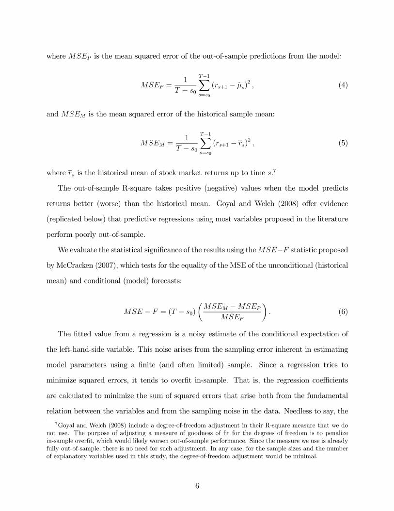
where is the mean squared error of the out-of-sample predictions from the model:
=1
− 0
−1X=0
(+1 − )2 (4)
and is the mean squared error of the historical sample mean:
=1
− 0
−1X=0
(+1 − )2 (5)
where is the historical mean of stock market returns up to time .7
The out-of-sample R-square takes positive (negative) values when the model predicts
returns better (worse) than the historical mean. Goyal and Welch (2008) offer evidence
(replicated below) that predictive regressions using most variables proposed in the literature
perform poorly out-of-sample.
We evaluate the statistical significance of the results using the− statistic proposedby McCracken (2007), which tests for the equality of the MSE of the unconditional (historical
mean) and conditional (model) forecasts:
− = ( − 0)
µ −
¶ (6)
The fitted value from a regression is a noisy estimate of the conditional expectation of
the left-hand-side variable. This noise arises from the sampling error inherent in estimating
model parameters using a finite (and often limited) sample. Since a regression tries to
minimize squared errors, it tends to overfit in-sample. That is, the regression coefficients
are calculated to minimize the sum of squared errors that arise both from the fundamental
relation between the variables and from the sampling noise in the data. Needless to say, the
7Goyal and Welch (2008) include a degree-of-freedom adjustment in their R-square measure that we do
not use. The purpose of adjusting a measure of goodness of fit for the degrees of freedom is to penalize
in-sample overfit, which would likely worsen out-of-sample performance. Since the measure we use is already
fully out-of-sample, there is no need for such adjustment. In any case, for the sample sizes and the number
of explanatory variables used in this study, the degree-of-freedom adjustment would be minimal.
6

second component is unlikely to hold robustly out-of-sample. Ashley (2006) shows that the
unbiased forecast is no longer squared-error optimal in this setting. Instead, the minimum-
MSE forecast represents a shrinkage of the unbiased forecast toward zero. This process
squares nicely with a prior of no predictability in returns. We apply a simple shrinkage
approach to the predictive regression coefficients in equation (2) suggested by Connor (1997)
as described in Appendix B.8
2.2 Return components
We decompose the total return of the stock market index into dividend yield and capital
gains:
1 ++1 = 1 + +1 ++1 (7)
=+1
++1
where +1 is the return obtained from time to time +1; +1 is the capital gain; +1
is the dividend yield; +1 is the stock price at time +1; and +1 is the dividend per share
paid during the return period.9
The capital gains component can be written as follows:
1 + +1 =+1
(8)
=+1+1
+1
=+1
+1
= (1 ++1)(1 ++1)
8Interestingly, shrinkage has been widely used in finance for portfolio optimization problems but not for
return forecasting. See Brandt (2009) for applications of shrinkage in portfolio management.9Bogle (1991a), Bogle (1991b), Fama and French (1998), Arnott and Bernstein (2002), and Ibbotson and
Chen (2003) offer similar decompositions of returns.
7

where +1 denotes earnings per share at time + 1; +1 is the price-earnings multiple;
+1 is the price-earnings multiple growth rate; and +1 is the earnings growth rate.
Instead of the price-earnings ratio, we could alternatively use any other price multiple
such as the price-dividend ratio, the price-to-book ratio, or the price-to-sales ratio. In these
alternatives, we must replace the growth in earnings by the growth rate of the denominator
in the multiple (i.e., dividends, book value of equity, or sales).10
The dividend yield can in turn be decomposed as follows:
+1 =+1
(9)
=+1
+1
+1
= +1(1 ++1)(1 ++1)
where +1 is the dividend-price ratio (which is distinct from the dividend yield in the
timing of the dividend relative to the price).
Replacing the capital gain and the dividend yield in equation (7), we can write the total
return as the product of the dividend-price ratio and the growth rates of the price-earnings
ratio and earnings:
1 ++1 = (1 ++1)(1 ++1) ++1(1 ++1)(1 ++1) (10)
= (1 ++1)(1 ++1)(1 ++1)
Finally, we make this expression additive by taking logs:
+1 = log(1 ++1) (11)
= +1 + +1 + +1
where lower-case variables denote log rates. Thus, log stock returns can be written as the
10In our empirical application we obtain similar findings using these three alternative price multiples.
8

sum of the growth in the price-earnings ratio, the growth in earnings, and the dividend-price
ratio.
2.3 The sum-of-the-parts method
We propose forecasting separately the components of the stock market return from equation
(11):
= + + (12)
We estimate the expected earnings growth using a 20-year moving average of the
growth in earnings per share up to time . This is consistent with the view that earnings
growth is nearly unforecastable (Campbell and Shiller (1988), Fama and French (2002), and
Cochrane (2008)) but has a low-frequency predictable component (Binsbergen and Koijen
(2010)) possibly due to a change over time in inflation (remember that earnings growth is a
nominal variable).
The expected dividend-price ratio is estimated by the current dividend-price ratio
(the logarithm of one plus the current dividend-price ratio). This implicitly assumes
that the dividend-price ratio follows a random walk as Campbell (2008) proposes.
The choice of estimators for earnings growth and dividend-price ratio is not entirely
uninformed. Indeed, we could be criticized for choosing the estimators with knowledge of
the persistence of earnings growth and dividend-price ratio. The concern is whether this
would have been known to an investor in the beginning of the sample, for example in the
1950s. We therefore check in a later section the robustness of our results to using different
window sizes for the moving average of earnings growth and estimating (out of sample) a
first-order auto-regression for the dividend-price ratio.
In the simplest version of the SOP method, we assume no multiple growth, i.e., = 0,
which fits closely with the random walk hypothesis for the dividend-price ratio. The SOP
9

method forecast at time of the stock return at time + 1 can thus be written as:
= + (13)
= + (14)
where is the 20-year moving average of the growth in earnings per share up to time , and
is the logarithm of one plus the current dividend-price ratio. This forecast looks like the
traditional predictive regression:
+1 = + + +1 (15)
with the restrictions that the intercept is set to and the slope is set to one.11
2.4 Results
We use the data set constructed by Goyal and Welch (2008), with monthly data to predict
the monthly stock market return and yearly data (non-overlapping) to predict the yearly
stock market return.12 The market return is proxied by the S&P 500 index continuously
compounded return including dividends. The sample period is from December 1927 to
December 2007 (or 1927 to 2007 with annual data).
Table 1 presents summary statistics of stock market return () and its components (,
, and ) at the monthly and yearly frequency. The mean annual stock market return
is 9.69% and the standard deviation is 19.42% over the whole sample period. Figure 1
plots the yearly cumulative realized components of stock market return over time. Clearly
average returns are driven mostly by earnings growth and the dividend-price ratio, while
most of the return volatility comes from earnings growth and the price-earnings ratio growth.
11We thank the referee for making this point and for suggesting the following analysis.12Goyal and Welch (2008) forecast the equity premium, i.e., the stock market return minus the short-term
riskless interest rate. In this paper, we forecast the market return but obtain similar results when we apply
our approach to the equity premium.
10

Figure 1 shows that the time series properties of the return components are very different.
The dividend-price ratio is very persistent, with an AR(1) coefficient of 0.79 at the annual
frequency, while the AR(1) coefficients of earnings growth and multiple growth are close to
zero.13
We perform an out-of-sample forecasting exercise along the lines of Goyal and Welch
(2008). We examine the out-of-sample performance of a long list of predictors of stock
returns. Appendix A provides a description of the predictors. Table 2 reports the results
for the whole sample period. The forecast period starts 20 years after the beginning of the
sample, i.e., in January 1948 and ends in December 2007 for monthly frequency (1948-2007
for yearly frequency). Panel A reports results for monthly return forecasts, and Panel B
reports results for annual return forecasts. Each row of the table uses a different forecasting
variable. The asterisks in the in-sample R-square column denote significance of the in-sample
regression as measured by the F-statistic. The asterisks in the out-of-sample R-squares
columns denote whether the performance of the conditional forecast is statistically different
from the unconditional forecasts (i.e., historical mean) using the McCracken (2007) MSE-F
statistic.
The in-sample R-square of the full-sample regression in Panel A show that most of the
variables have modest predictive power for monthly stock returns over the long sample period
considered here. The most successful variable is net equity expansion with an R-square of
1.07%. Overall, there are only four variables significant at the 5% level.
The remaining two columns evaluate the out-of-sample performance of the different fore-
casts using the out-of-sample R-square relative to the historical mean. The fourth column
reports the out-of-sample R-squares from the traditional predictive regression approach as
in Goyal and Welch (2008). The fifth column reports the out-of-sample R-squares from
the predictive regression with shrinkage. We present the out-of-sample R-squares from the
13Earnings growth shows substantial persistence at the monthly frequency, but that is because we measure
earnings over the previous 12 months, and there is therefore substantial overlap in the series from one month
to the next.
11

sum-of-the-parts method (SOP) method with no multiple growth at the bottom of the panel.
Several conclusions stand out for the monthly return forecasts in Panel A. First, consistent
with the findings in Goyal and Welch (2008), out-of-sample R-squares from the traditional
predictive regression are in general negative, ranging from -1.78% to -0.05%. The one excep-
tion is the net equity expansion variable, which presents an out-of-sample R-square of 0.69%
(significant at the 1% level).
Second, shrinkage improves the out-of-sample performance of most predictors. In the
next column there are now 8 variables with positive R-squares out of 16 variables, although
only two are significant at the 5% level. The R-squares are, however, still modest, with a
maximum of 0.53%.
We next perform the out-of-sample forecasting exercise using the simplest version of the
SOP method. Using only the dividend price and earnings growth components to forecast
monthly stock market returns, we obtain an out-of-sample R-square of 1.32% (significant
at the 1% level), which is much better than the performance of the traditional predictive
regressions.
We now look at the annual stock market return forecasts. We use non-overlapping returns
to avoid the concerns with the measurement of R-squares with overlapping returns pointed
out by Valkanov (2003) and Boudoukh, Richardson, and Whitelaw (2008). Our findings for
monthly return forecasts are also valid at the annual frequency: forecasting the components
of stock market returns separately delivers out-of-sample R-squares significantly higher than
traditional predictive regressions. There is an even more striking improvement at the yearly
frequency.
The traditional predictive regression R-squares in Panel B are in general negative at yearly
frequency (13 out of 16 variables) consistent with Goyal and Welch (2008). The R-squares
range from -17.57% to 7.54%, but only one variable is significant at the 1% level. Using
shrinkage with traditional predictive regressions (next column) produces 11 variables with
positive R-squares, but only 2 are significant at the 5% level. Forecasting the components of
12

stock market returns separately dramatically improves performance. We obtain an R-square
of 13.43% (significant at the 1% level) with the SOP method to forecast annual stock market
returns in Panel B.
We compare the performance of the SOP method with the historical mean and predictive
regression methods of forecasting stock market returns using graphical analysis. The aim is
to understand better why the SOP method outperforms the alternative methods. We present
and discuss the results at the annual frequency but the conclusions are qualitatively similar
using the monthly frequency.
Figure 2 shows the SOP forecast of stock market return with no multiple growth and
its two components. We see substantial time variation in the stock market return forecasts
over time, from nearly 4% per year around the year of 2000 to almost 15% per year in
the early 1950s and the 1970s. The time variation of expected stock market return is due
to both components. The SOP implicit equity premium in the middle panel also shows
ample variability over time, ranging from approximately -2% to 13%. Interestingly, the
equity premium was high in the early 1950s and slightly negative in the early 1980s when
the stock market return forecast reached the highest figure but interest rates were also at
record high levels. The bottom panel shows that the SOP forecast aligns with subsequent
five-year average realized returns with the exception of the late 1940s (post World War II
economic growth surprise), early 1970s (oil shock), and mid 1990s (internet bubble). In our
forecast period, the average SOP return forecast of 9.52% is below the average realized stock
market return of 11.28%, which is consistent with returns in this period having a positive
surprise component. The SOP implicit equity premium is significantly negatively correlated
with interest rates (TBL and TMS) and positively correlated with the default spread (DFY)
– the R-square of a regression of the SOP equity premium on the default spread is 45%
(untabulated results).
Figure 3 compares the return forecasts from the SOP method with forecasts from tradi-
tional predictive regressions and the historical mean. We see that there are large differences
13

in the three forecasts. The expected returns using predictive regressions change drastically
depending on the predictor used. The historical mean and, to some extent, the predictive
regressions tend to increase with past returns. Thus, after a large run up in the market
(as in 1995-2000), these two methods forecast higher returns. The opposite happens with
the SOP method since after a run up the dividend-price ratio tends to be low. The first
panel displays return forecasts from a predictive regression on the dividend-price ratio. It
is interesting to notice the large difference between this forecast and the SOP forecast that
relies on the same dividend-price ratio. This difference is driven by the regression coefficient
estimates, which we will analyze in detail in the next subsection.
Figure 4 shows cumulative out-of-sample R-squares for both the SOP method and pre-
dictive regressions. The SOP method dominates over the whole sample period, with good
fit, although there has been a drop in predictability over time.
2.5 Discussion
The SOPmethod looks like a predictive regression with the dividend-price ratio as a predictor
and with the restrictions that the intercept equals the earnings growth historical average and
the slope equals one. A concern with the SOP method is that we might have picked, by
chance, coefficients that are close to the in-sample estimates of the predictive regression (15)
over the forecasting period. In that case, the out-of-sample R-square would really be an
in-sample R-square.
We address this concern by estimating the (in sample) predictive regression (15) with
annual returns over the forecasting period 1948-2007. We obtain an estimate of -0.018,
which compares with a of 0.062 (average in the 1948-2007 period), and a estimate of 3.747,
which compares with a of one in the SOP method. Clearly the coefficients of the predictive
regression are very different from the coefficients implicit in the SOPmethod. To compare the
explanatory power of this predictive regression with the out-of-sample results obtained with
the SOP method, we compute a pseudo out-of-sample R-square of the predictive regression
14
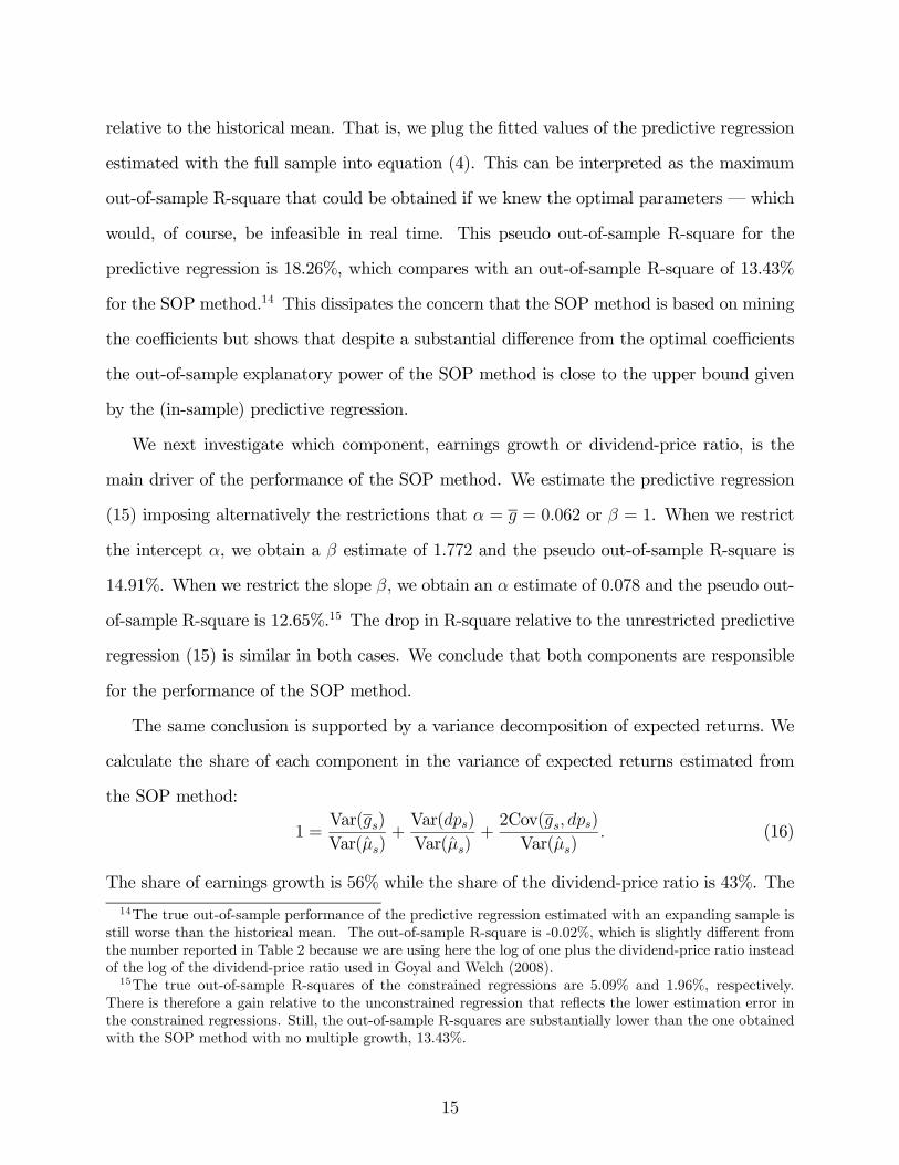
relative to the historical mean. That is, we plug the fitted values of the predictive regression
estimated with the full sample into equation (4). This can be interpreted as the maximum
out-of-sample R-square that could be obtained if we knew the optimal parameters – which
would, of course, be infeasible in real time. This pseudo out-of-sample R-square for the
predictive regression is 18.26%, which compares with an out-of-sample R-square of 13.43%
for the SOP method.14 This dissipates the concern that the SOP method is based on mining
the coefficients but shows that despite a substantial difference from the optimal coefficients
the out-of-sample explanatory power of the SOP method is close to the upper bound given
by the (in-sample) predictive regression.
We next investigate which component, earnings growth or dividend-price ratio, is the
main driver of the performance of the SOP method. We estimate the predictive regression
(15) imposing alternatively the restrictions that = = 0062 or = 1. When we restrict
the intercept , we obtain a estimate of 1.772 and the pseudo out-of-sample R-square is
14.91%. When we restrict the slope , we obtain an estimate of 0.078 and the pseudo out-
of-sample R-square is 12.65%.15 The drop in R-square relative to the unrestricted predictive
regression (15) is similar in both cases. We conclude that both components are responsible
for the performance of the SOP method.
The same conclusion is supported by a variance decomposition of expected returns. We
calculate the share of each component in the variance of expected returns estimated from
the SOP method:
1 =Var()
Var()+Var()
Var()+2Cov( )
Var() (16)
The share of earnings growth is 56% while the share of the dividend-price ratio is 43%. The
14The true out-of-sample performance of the predictive regression estimated with an expanding sample is
still worse than the historical mean. The out-of-sample R-square is -0.02%, which is slightly different from
the number reported in Table 2 because we are using here the log of one plus the dividend-price ratio instead
of the log of the dividend-price ratio used in Goyal and Welch (2008).15The true out-of-sample R-squares of the constrained regressions are 5.09% and 1.96%, respectively.
There is therefore a gain relative to the unconstrained regression that reflects the lower estimation error in
the constrained regressions. Still, the out-of-sample R-squares are substantially lower than the one obtained
with the SOP method with no multiple growth, 13.43%.
15
covariance between the earnings growth and the dividend-price ratio has a share of only
1%. These results indicate that both components contribute significantly and approximately
with the same magnitude to the estimated expected returns. Our results are not driven by
a single component.
The SOP method assumes that the persistence of the dividend-price ratio is very high
and that the persistence of earnings growth is close to nil. This is implicit in forecasting
the future dividend-price ratio with the current level of the ratio and in forecasting earnings
growth with a 20-year moving average. Thus, another concern with the SOP method is that
investors might not have known these facts about the persistence of earnings growth and of
the dividend-price ratio at earlier times in the sample. In that case, the SOP method could
not have been used in real time since the 1950s. We now investigate the sensitivity of the
SOP method to these implicit assumptions.
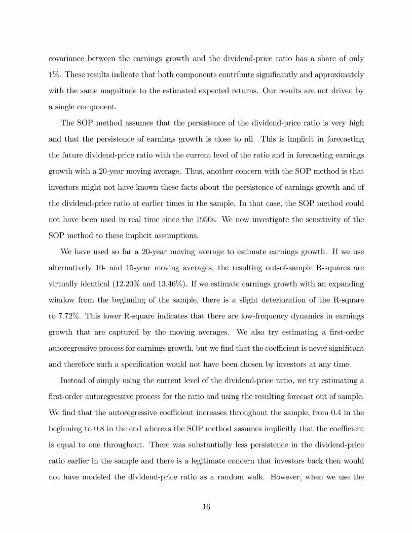
We have used so far a 20-year moving average to estimate earnings growth. If we use
alternatively 10- and 15-year moving averages, the resulting out-of-sample R-squares are
virtually identical (12.20% and 13.46%). If we estimate earnings growth with an expanding
window from the beginning of the sample, there is a slight deterioration of the R-square
to 7.72%. This lower R-square indicates that there are low-frequency dynamics in earnings
growth that are captured by the moving averages. We also try estimating a first-order
autoregressive process for earnings growth, but we find that the coefficient is never significant
and therefore such a specification would not have been chosen by investors at any time.
Instead of simply using the current level of the dividend-price ratio, we try estimating a
first-order autoregressive process for the ratio and using the resulting forecast out of sample.
We find that the autoregressive coefficient increases throughout the sample, from 0.4 in the
beginning to 0.8 in the end whereas the SOP method assumes implicitly that the coefficient
is equal to one throughout. There was substantially less persistence in the dividend-price
ratio earlier in the sample and there is a legitimate concern that investors back then would
not have modeled the dividend-price ratio as a random walk. However, when we use the
16

autoregressive forecast of the dividend-price ratio as an alternative to the current ratio, we
obtain an out-of-sample R-square as high as before, 12.47%. We conclude that the SOP
method still works well even if we take into account a level of persistence in the dividend-
price ratio well below a unit root.
It is instructive to compare our results to those in Campbell and Thompson (2008). They
show that imposing restrictions on the signs of the coefficients of the predictive regressions
modestly improves out-of-sample performance in both statistical and economic terms. More
important, they suggest using the Gordon growth model to decompose expected stock returns
(where earnings growth is entirely financed by retained earnings). Their method is a special
case of our equation (12) with b = 0 and b = (1−DE)– i.e., expected plowback
times return on equity. The last component assumes that earnings growth corresponds to
retained earnings times the return on equity. It is implicitly assumed that there are no
external financing flows and that the marginal investment opportunities earn the same as
the average return on equity.
Campbell and Thompson (2008) use historical averages to forecast the plowback (or one
minus the payout ratio) and the return on equity. We implement their method in our sample
and the out-of-sample R-square is 0.54% (significant at the 5% level) with monthly frequency
and 3.24% (significant only at the 10% level) with yearly frequency.16 Our method using
only the dividend-price ratio and earnings growth components gives significantly higher R-
squares: 1.32% with monthly frequency and 13.43% with yearly frequency. In summary,
the SOP substantially improves the out-of-sample explanatory power relative to previous
studies, and the magnitude of this improvement is economically meaningful for investors.
16Campbell and Thompson (2008) use a longer sample period from 1891 to 2005 (with forecasts begin-
ning in 1927) and obtain out-of-sample R-squares of 0.63% with monthly frequency and 4.35% with yearly
frequency. We thank John Campbell for providing their data and programs for this comparison.
17
3. Extensions and Robustness
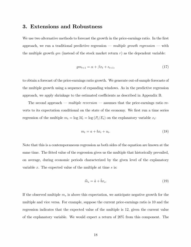
We use two alternative methods to forecast the growth in the price-earnings ratio. In the first
approach, we run a traditional predictive regression – multiple growth regression – with
the multiple growth (instead of the stock market return ) as the dependent variable:
+1 = + + +1 (17)
to obtain a forecast of the price-earnings ratio growth. We generate out-of-sample forecasts of
the multiple growth using a sequence of expanding windows. As in the predictive regression
approach, we apply shrinkage to the estimated coefficients as described in Appendix B.
The second approach – multiple reversion – assumes that the price-earnings ratio re-
verts to its expectation conditional on the state of the economy. We first run a time series
regression of the multiple = log = log () on the explanatory variable :
= + + (18)
Note that this is a contemporaneous regression as both sides of the equation are known at the
same time. The fitted value of the regression gives us the multiple that historically prevailed,
on average, during economic periods characterized by the given level of the explanatory
variable . The expected value of the multiple at time is:
b = + (19)
If the observed multiple is above this expectation, we anticipate negative growth for the
multiple and vice versa. For example, suppose the current price-earnings ratio is 10 and the
regression indicates that the expected value of the multiple is 12, given the current value
of the explanatory variable. We would expect a return of 20% from this component. The
18

estimated regression residual gives an estimate of the expected growth in the price multiple:
− = b − (20)
=
In practice, the reversion of the multiple to its expectation is quite slow, and does not
take place in a single period. To take this into account, we run a second regression of the
realized multiple growth on the expected multiple growth using the estimated residuals from
regression equation (18):
+1 = + (−) + (21)
Finally, we use these coefficients (after applying shrinkage as described in Appendix B)
to forecast as:
= b+ b (−) (22)
We generate out-of-sample forecasts of the multiple growth using a sequence of expanding
windows.
Table 3 reports the results for the whole sample period of these extensions of the SOP
method. We use the same predictors to forecast the multiple growth in the sum-of-
the-parts (SOP) method than in predictive regressions. In the SOP method with multiple
reversion we do not use the predictors that directly depend on the stock index price (EP,
SEP, DP, DY, and BM) as this would correspond to explaining the price-earnings multiple
with other multiples.
Panel A reports results for monthly return forecasts and Panel B reports results for
annual return forecasts. The R-squares in the SOP method with multiple growth regression
in Panel A are all positive and range from 0.68% (book-to-market) to 1.55% (net equity
expansion). Several variables turn in a good performance with R-squares above 1.3%, such
as the term spread, inflation, T-bill rate, and the default yield spread. All the SOP method
19
forecast results are significant at the 1% level under the McCracken (2007) MSE-F statistic.
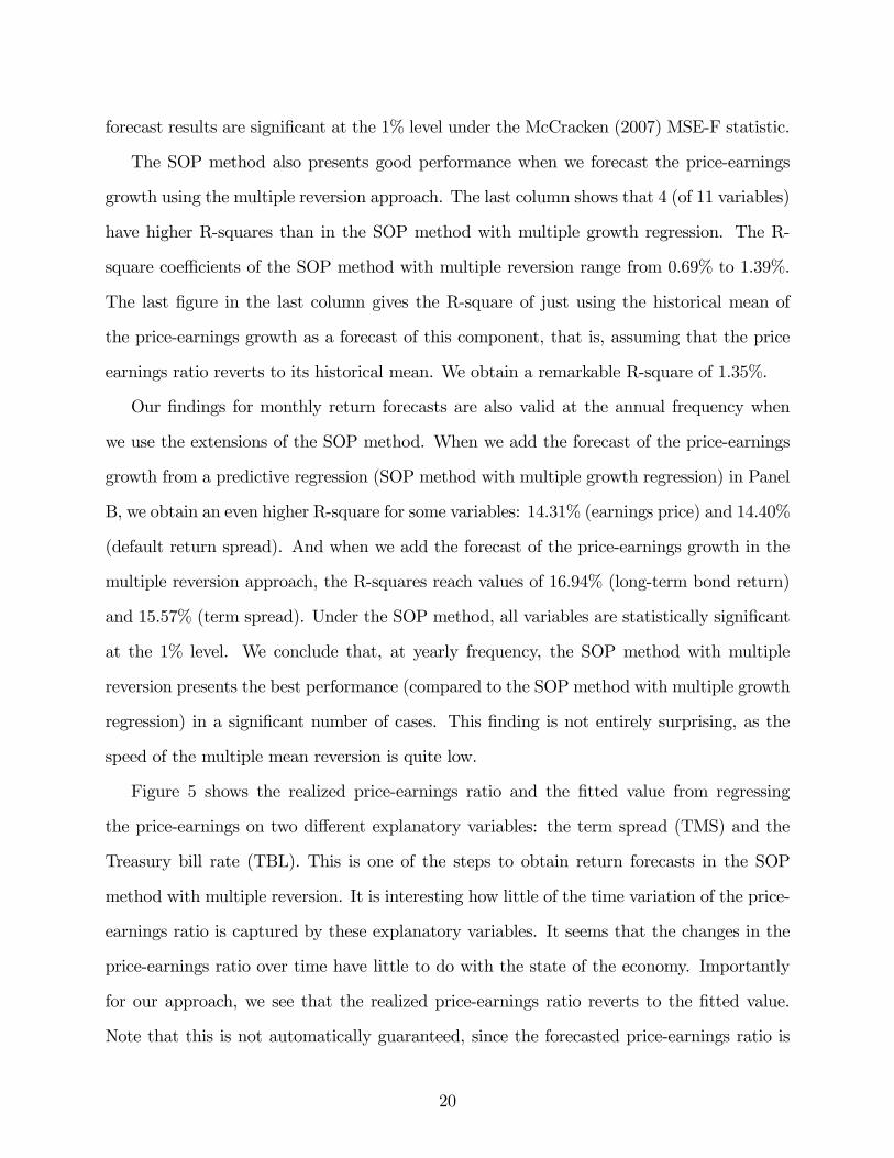
The SOP method also presents good performance when we forecast the price-earnings
growth using the multiple reversion approach. The last column shows that 4 (of 11 variables)
have higher R-squares than in the SOP method with multiple growth regression. The R-
square coefficients of the SOP method with multiple reversion range from 0.69% to 1.39%.
The last figure in the last column gives the R-square of just using the historical mean of
the price-earnings growth as a forecast of this component, that is, assuming that the price
earnings ratio reverts to its historical mean. We obtain a remarkable R-square of 1.35%.
Our findings for monthly return forecasts are also valid at the annual frequency when
we use the extensions of the SOP method. When we add the forecast of the price-earnings
growth from a predictive regression (SOP method with multiple growth regression) in Panel
B, we obtain an even higher R-square for some variables: 14.31% (earnings price) and 14.40%
(default return spread). And when we add the forecast of the price-earnings growth in the
multiple reversion approach, the R-squares reach values of 16.94% (long-term bond return)
and 15.57% (term spread). Under the SOP method, all variables are statistically significant
at the 1% level. We conclude that, at yearly frequency, the SOP method with multiple
reversion presents the best performance (compared to the SOP method with multiple growth
regression) in a significant number of cases. This finding is not entirely surprising, as the
speed of the multiple mean reversion is quite low.
Figure 5 shows the realized price-earnings ratio and the fitted value from regressing
the price-earnings on two different explanatory variables: the term spread (TMS) and the
Treasury bill rate (TBL). This is one of the steps to obtain return forecasts in the SOP
method with multiple reversion. It is interesting how little of the time variation of the price-
earnings ratio is captured by these explanatory variables. It seems that the changes in the
price-earnings ratio over time have little to do with the state of the economy. Importantly
for our approach, we see that the realized price-earnings ratio reverts to the fitted value.
Note that this is not automatically guaranteed, since the forecasted price-earnings ratio is
20
not the fitted value of a regression estimated ex post but is constructed from a series of
regressions estimated with data up to each time. Yet the reversion is quite slow and at
times takes almost ten years. The second regression in equation (21) captures this speed
of adjustment. The expected return coming from the SOP method with multiple reversion
varies substantially over time and takes both positive and negative values.
Figure 6 shows the three versions of the SOP forecasts with two alternative predictive
variables (TMS and TBL). Of course, the forecasts under the SOP method with no multiple
growth are the same in the three panels. The three versions of the SOP method are highly
correlated, but the SOP with multiple reversion displays more variability.
3.1 Subperiods
As Goyal and Welch (2008) find that predictive regressions perform particularly poor in
the last decades, we repeat our out-of-sample performance analysis using two subsamples
that divide the forecasting period in halves: from January 1948 through December 1976
and from January 1977 through December 2007. As before, forecasts begin 20 years after
the subsample start. Table 4 presents the results. Panels A.1 and A.2 present results using
monthly returns and Panels B.1 and B.2 results using annual returns (non-overlapping).
Like Goyal and Welch (2008), we also find better out-of-sample performance in the first
subsample (which includes the Great Depression and World War II) than in the second
subsample (which includes the oil shock of the 1970s and the internet bubble at the end of
the 20th Century). The sum-of-the-parts (SOP) method dominates the traditional predic-
tive regressions in both subsamples and provides significant gains in performance over the
historical mean.
Using monthly data, the out-of-sample R-squares of the traditional predictive regression
are in general negative, ranging from -2.20% to 0.37% in the first subperiod and from -2.09%
to 0.53% in the second subperiod. Net equity expansion has the best performance in both
subperiods, and it is the only significant variable at the 5% level.
21
In both subperiods, there is a very significant improvement in the out-of-sample fore-
casting performance when we separately model the components of the stock market return.
As before, a considerable part of the improvement comes from the dividend-price ratio and
earnings growth components alone: out-of-sample R-square of 1.80% in the first subperiod
and 0.98% in the second subperiod (both significant at the 5% level) at the monthly fre-
quency. The maximum R-squares using the SOP method with multiple growth regression
are 2.29% in the first subperiod and 1.44% in the second subperiod (both significant at the
1% level). This is much better than the performance of the traditional predictive regressions.
There is similar good performance when we use the SOP method with multiple reversion.
The maximum R-squares are roughly 2% (in the first subperiod) and 1% (in the second
subperiod), and they are all significant at the 5% level with one exception.
At the annual frequency, we find that most variables perform more poorly in the most
recent subperiod. Using annual data, the out-of-sample R-squares of the traditional pre-
dictive regressions are in general negative in both subperiods. Forecasting the components
of stock market returns separately, however, delivers positive and significant out-of-sample
R-squares in both subperiods. As before, a considerable part of the improvement comes from
the dividend-price ratio and earnings growth components alone. We obtain out-of-sample R-
squares of 14.66% in the first subperiod and 12.10% in the second subperiod. The maximum
R-squares using the SOP method with multiple growth regression are higher than 20% in
the first subperiod and higher than 15% in the second subperiod (both significant at the 1%
level). This is much better than the performance of the traditional predictive regressions.
3.2 Trading strategies
To assess the economic importance of the different approaches to forecast returns, we run
out-of-sample trading strategies that combine the stock market with the risk-free asset. Each
period, we use the different estimates of expected returns to calculate the Markowitz optimal
22

weight on the stock market:
= − +1
b2 (23)
where +1 denotes the risk-free return from time to + 1 (which is known at time ),
is the risk-aversion coefficient assumed to be 2, and b2 is the variance of the stock marketreturns that we estimate using all the available data up to time .17 The only thing that varies
across portfolio policies are the estimates of the expected returns either from the predictive
regressions or the sum-of-the-parts (SOP) method. Note that these portfolio policies could
have been implemented in real time with data available at the time of the decision.18
We then calculate the portfolio return at the end of each period as:
+1 = +1 + (1− )+1 (24)
We iterate this process until the end of the sample , thereby obtaining a time series of
returns for each trading strategy.
To evaluate the performance of the strategies, we calculate their certainty equivalent
return:
= −
22() (25)
where is the sample mean portfolio return, and 2() is the sample variance portfolio
return. This is the risk-free return that a mean-variance investor with a risk-aversion coeffi-
cient would consider equivalent to investing in the strategy. The certainty equivalent gain
can also be interpreted as the fee the investor would be willing to pay to use the information
in each forecast model. We also calculate the gain in Sharpe ratio (annualized) for each
strategy.
17Given the average stock market excess return and variance, a mean-variance investor with risk-aversion
coefficient of 2 would allocate all wealth to the stock market. This is therefore consistent with equilibrium
with this representative investor. Results are similar when we use other values for the risk-aversion coefficient.18In untabulated results, we obtain slightly better certainty equivalents and Sharpe ratio gains if we
impose portfolio constraints preventing investors from shorting stocks ( ≥ 0%) and assuming more than50% leverage ( ≤ 150%).
23

Table 5 reports the certainty equivalent gains (annualized and in percentage) relative to
investing based on the historical mean. Using the historical mean, the certainty equivalents
are 7.4% and 6.4% per year at monthly and yearly frequencies, respectively. Using traditional
predictive regressions leads to losses compared to the historical mean in most cases. Applying
shrinkage to the traditional predictive regression slightly improves the performance of the
trading strategies.
The SOP method always leads to economic gains relative to the historical mean. In
fact, using only the dividend-price ratio and earnings growth components, we obtain an
economic gain of 1.79% per year. The greatest gains in the SOP method with multiple
growth regression and multiple reversion are 2.33% and 1.72% per year. We obtain similar
results using annual (non-overlapping) returns.
Table 6 reports the gains in Sharpe ratio over investing using the historical mean. For the
historical mean, the Sharpe ratios are 0.45 and 0.30 at the monthly and annual frequency,
respectively. We find once again that using traditional predictive regressions leads to losses
compared to the historical mean in most cases. Applying shrinkage to the traditional pre-
dictive regression slightly improves the performance of the trading strategies.
The SOP method always leads to Sharpe ratio gains relative to the historical mean. In
fact, using only the dividend-price ratio and earnings growth components (SOP method
with no multiple growth), we obtain a Sharpe ratio gain of 0.31. The maximum gains in the
multiple growth regression and multiple reversion approaches are 0.33 and 0.24. We obtain
similar Sharpe ratio gains using annual (non-overlapping) returns.
3.3 International evidence
We repeat the analysis using international data. We obtain data on stock price indices and
dividends from Global Financial Data (GFD) for the U.K. and Japan, which are the two
largest stock markets in the world after the U.S. The sample period is from 1950 through
2007, which is shorter than the one in Tables 2 and 3 because of data availability. We
24

report results using stock market returns in local currency at the annual frequency, but we
obtain similar results using returns at the monthly frequency or returns in U.S. dollars. We
consider three macroeconomic variables (long-term yield, term spread, and Treasury bill rate
also obtained from GFD) and the dividend yield as predictors because these are the variable
that are available for the longest sample period. We apply here the sum-of-the-parts (SOP)
method using price-dividend ratio as the price multiple rather than the price-earnings ratio
because earnings for the U.K. and Japan are available only for a shorter period.
Table 7 presents the results for the international data. Panels A and B present the results
for the U.K. and Japan, and Panel C presents the results for the U.S. in the comparable
sample period (1950-2007) and using the price-dividend ratio as multiple. The traditional
predictive regression R-squares are in general negative, consistent with our previous findings.
The R-squares range from -47.54% to 3.12%, and none is significant at the 5% level. Using
shrinkage with the traditional prediction regression improves performance, and the R-square
for the dividend yield is now significant at the 5% level in the U.K. and Japan (at only the
10% level in the U.S.).
Forecasting the components of stock market returns separately dramatically improves
performance. We obtain R-squares of 10.73% and 12.14% (both significant at the 1% level)
in the U.K. and Japan when we use only the dividend-price ratio and dividend growth com-
ponents to forecast stock market returns (SOP method with no multiple growth). When
we add the forecast of the price-dividend ratio growth from a predictive regression (SOP
method with multiple growth regression), we obtain an even higher R-square for some vari-
ables: 13.28% in the U.K. using the dividend yield. When we alternatively add the forecast
of the price-dividend ratio growth from the multiple reversion approach, the R-squares reach
values of more than 11% in the U.K. and in Japan. Under the SOP method with multiple
reversion, all variables are statistically significant at the 5% level. Interestingly, the SOP
method performs better in the U.K. and in Japan than in the U.S. when we redo the analysis
for the comparable sample period and using the price-dividend ratio as the multiple (Panel
25

C). The SOP method clearly dominates predictive regressions in U.S. data.
Figure 7 shows forecasts of stock market return for the U.K., Japan, and the U.S. accord-
ing to the SOP method (with no multiple growth). There are substantial differences. The
U.K. generally offers the highest expected returns (around 11.8% on average), while expected
returns in Japan are the lowest through most of the sample (4.7% on average). At times,
the difference in return forecasts across countries is as high as 12 percentage points. There
is more variability in return forecasts in the U.K. and Japan than in the U.S. Interestingly,
the correlation between expected returns in the U.K. and the U.S. is high (on the order of
0.7), but Japanese expected returns are negatively correlated with both the U.K. and U.S.
stock markets (on the order of -0.3).
3.4 Analyst forecasts
An alternative forecast of earnings can be obtained from analyst estimates drawn from IBES
and aggregated across all S&P 500 stocks. We use these forecasts to calculate both the price
earnings ratio and the earnings growth. Panel A of Table 8 reports the results for the sample
period from January 1982 (when IBES data starts) through December 2007 with monthly
frequency. In this exercise we begin forecasts 5 years after the sample start, rather than 20
years as we did before, because of the shorter sample. Panel B replicates the analysis of
Tables 2 and 3 for the same sample period for comparison.
We find that analyst forecasts work quite well with out-of-sample R-squares between
1.70% and 3.10%. However, the SOP method based only on historical data growth works
even better than based on analyst forecasts in this sample period, with out-of-sample R-
squares between 2.81% and 4.66%. This is consistent with the well-known bias in analyst
forecasts.
26

4. Simulation analysis
In this section, we conduct a Monte Carlo simulation experiment to better understand the
performance of the sum-of-the-parts (SOP) method. We simulate the economy in Binsbergen
and Koijen (2010) where expected returns () and expected dividend growth rates () follow
AR(1) processes:
+1 = 0 + 1( − 0) + +1 (26)
+1 = 0 + 1( − 0) + +1 (27)
The dividend growth rate is equal to the expected dividend growth rate plus an orthogonal
shock:
∆+1 = + +1 (28)
The Campbell and Shiller (1988) log-linear present value model implies that:
+1 = + (+1 − +1) +∆+1 − ( − ) (29)
where and are constants of the log linearization.
Iterating equation (29) and using processes (26)-(28), it follows that:
− = −1( − 0) +2( − 0) (30)
where = 1− +
0−01− 1 =
11−1 and 2 =
11−1 .
We simulate returns, dividend growth, and the dividend-price ratio from these equations
using the estimated parameter values in Table II of Binsbergen and Koijen (2010). Since
the AR(1) process for expected dividend growth rates in (27) can be written as an infinite
moving average model, there is predictability of dividend growth by a smoothed average of
past growth rates in this model.
We simulate 10,000 samples of 80 years (which is approximately the size of our empirical
27

sample) of returns, dividend growth, and the dividend-price ratio for this economy. We use
the simulated data to study the different forecasting methods of stock market return. The
advantage of using Monte Carlo simulation is that we know the true expected return at each
particular time. Thus, we can compare our forecasts with (true) expected returns and not
just with realized returns as we do in the empirical analysis.
In each simulation of the economy, we replicate our out-of-sample empirical analysis; that
is, we compute for each year the forecast of returns from the three approaches (historical
mean, predictive regression, and SOP method with no multiple growth) using only past data.
The regressions use the log dividend-price ratio as predictive variable.
Figure 8 shows a scatter plot of each estimator of expected returns versus the true ex-
pected returns at the end of the simulated samples. The SOP expected return estimates
have the lowest bias and variance.19 The historical mean also has a low variance but it does
not capture the variation in the true expected returns. Predictive regressions have poor
performance in terms of predicting stock market returns, with a higher variance than the
SOP and historical mean methods.
To quantify this analysis, we compute the sum of the squares of the difference between
the estimates of expected returns and the true expected returns from the simulation. Panel
A of Table 9 presents the mean and the percentiles (across simulations) of the root mean
square error (RMSE) of each forecast method. The results clearly show that the SOP
method yields a better estimate of expected returns than both predictive regressions and the
historical mean of returns. The average RMSE of the SOP method is 2.87%, which is low in
absolute terms and significantly lower than the RMSE of the historical mean and predictive
regressions, 4.94% and 3.73%, respectively. This difference persists across all the percentiles
of the distribution of the RMSE.
19There is a slight “smile” shape in the relation between the true expected returns and the SOP estimates of
expected returns. This happens because we simulate expected returns from a Campbell-Shiller approximation
where there is a linear relation between expected returns and the log of the dividend-price ratio. The
corresponding relation in the decomposition underlying the SOP is between expected returns and the log of
one plus the dividend price ratio. The difference between the log of the ratio and the log of one plus the
ratio explains the non-linearity in the plot.
28

We can decompose the expected MSE (across simulations) of each estimator of expected
returns in the following way:
1
− 0
−1X=0
E£( − )
2¤ =1
− 0
−1X=0
[E ( − )]2 +
1
− 0
−1X=0
Var ()
+1
− 0
−1X=0
Var ()−1
− 0
−1X=0
2Cov ( ) (31)
where E(·), Var(·), and Cov(·) are moments across simulations. The first term corresponds tothe square of the bias of the estimates of expected returns. The second term is the variance
of the estimates of expected returns. The third term is the variance of the true expected
return (which is the same for all methods). The final term is the covariance between the
estimates of expected returns and the true expected return. Panel B of Table 9 presents the
results of this decomposition of the MSE in the simulation exercise.
While the bias squared component of all estimates of expected returns is insignificant,
the variance of the predictive regression estimates of expected returns is more than five
times larger than the variance of the SOP estimates. This variance, due to estimation error,
is therefore the main weakness of predictive regressions. The historical mean estimates
of expected returns present a variance slightly lower than the SOP estimates. Regarding
the covariance term, the SOP and predictive regressions estimates of expected return have
significant positive correlations with the true expected return, which contribute to reducing
the MSE. In contrast, the historical mean is actually negatively correlated with the true
expected return, which adds to its MSE. Overall, the superior performance of the SOP
method relative to the predictive regression comes from its lower variance and its higher
correlation with the true expected return. The superior performance of the SOP method
relative to the historical mean its explained by its much higher correlation with the true
expected return.
Finally, we compute out-of-sample R-squares in the simulations. For predictive regres-
sions and the SOP method, the R-squares are 4.03% and 7.17%, respectively. These values
29

compare with an R-square of 10.74% for the true expected return, which constitutes an
upper bound for this statistic. The SOP method is close to being as efficient as the true ex-
pected return (which is obviously unfeasible outside of simulation experiments) in predicting
returns.
5. Conclusion
We propose forecasting separately the dividend-price ratio, the earnings growth, and the
price-earnings growth components of stock market returns – the sum-of-the-parts (SOP)
method. Our method exploits the different time-series properties of the components. We
apply the SOP method to forecast stock market returns out-of-sample over 1927-2007. The
SOP method produces statistically and economically significant gains for investors and per-
forms better out-of-sample than the historical mean or predictive regressions. The gain
in performance of the SOP method relative to predictive regressions is mainly due to the
absence of estimation error.
Our results have important consequences for corporate finance and investments. The
SOP forecasts of the equity premium can be used for cost of capital calculations in project
and firm valuation. The results presented suggest that discount rates and corporate decisions
should depend more on market conditions. In the investment world, we show that there are
important gains from timing the market. Of course, to the extent that what we are capturing
is excessive predictability rather than a time-varying risk premium, the success of our analysis
will eventually destroy its usefulness. Once enough investors follow our approach to predict
returns, they will impact market prices and again make returns unpredictable.
30

Appendix A. Definition of Predictors
The predictors of stock returns are:
Stock variance (SVAR): sum of squared daily stock market returns on the S&P 500.
Default return spread (DFR): difference between long-term corporate bond and long-term
bond returns.
Long-term yield (LTY): long-term government bond yield.
Long-term return (LTR): long-term government bond return.
Inflation (INFL): growth in the Consumer Price Index with a one-month lag.
Term spread (TMS): difference between the long-term government bond yield and the T-
bill.
Treasury bill rate (TBL): three-month Treasury bill rate.
Default yield spread (DFY): difference between BAA- and AAA-rated corporate bond
yields.
Net equity expansion (NTIS): ratio of 12-month moving sums of net issues by NYSE-listed
stocks to NYSE market capitalization.
Return on equity (ROE): ratio of 12-month moving sums of earnings to book value of equity
for the S&P 500.
Dividend payout ratio (DE): difference between the log of dividends (12-month moving
sums of dividends paid on S&P 500) and the log of earnings (12-month moving sums
of earnings on S&P 500).
Earnings price ratio (EP): difference between the log of earnings (12-month moving sums
of earnings on S&P 500) and the log of prices (S&P 500 index price).
31

Smooth earnings price ratio (SEP): 10-year moving average of earnings-price ratio.
Dividend price ratio (DP): difference between the log of dividends (12-month moving sums
of dividends paid on S&P 500) and the log of prices (S&P 500 index price).
Dividend yield (DY): difference between the log of dividends (12-month moving sums of
dividends paid on S&P 500) and the log of lagged prices (S&P 500 index price).
Book-to-market (BM): ratio of book value to market value for the Dow Jones Industrial
Average.
Appendix B. Shrinkage Approach
Following Connor (1997), we transform the estimated coefficients of the predictive regression
in equation (2) by:
∗ =
+ (32)
∗ = − ∗ (33)
where is the historical mean of the predictor up to time . In this way, the slope coeffi-
cient is shrunk toward zero, and the intercept changes to preserve the unconditional mean
return. The shrinkage intensity can be thought of as the weight given to the prior of no
predictability. It is measured in units of time periods. Thus, if is set equal to the number
of data periods in the data set , the slope coefficient is reduced by half. Connor (1997)
shows that it is optimal to choose = 1, where is the expectation of a function of the
regression R-square:
= E
µ2
1−2
¶≈ E(2) (34)
This is the expected explanatory power of the model. We use = 100 with yearly
data and = 1 200 with monthly data. This would give a weight of 100 years of data to
32

the prior of no predictability. Alternatively, we can interpret this as an expected R-square
of approximately 1% for predictive regressions with yearly data and less than 0.1% with
monthly data, which seems reasonable in light of findings in the literature. This means that
if we run the predictive regression with 30 years of data, the slope coefficient is shrunk to
23% (= 30(100 + 30)) of its estimated size.
Finally, we use these coefficients to forecast the stock market return as:
= ∗ + ∗ (35)
As in the predictive regression approach in equations (32)-(34), we apply shrinkage to
the estimated coefficients of the multiple growth regression in equation (17):
∗ =
+ (36)
∗ = −∗ (37)
which makes the unconditional mean of the multiple growth equal to zero.
We also apply shrinkage to the estimated coefficients of the regression of the realized
multiple growth on the expected multiple growth in equation (21) as follows:
∗ =
+ (38)
∗ = −∗ ¡−¢ (39)
= ∗ (40)
where is the sample mean of the regression residuals up to time (not necessarily equal
to zero). This assumes that the unconditional expectation of the multiple growth is equal
to zero. That is, with no information about the state of the economy, we do not expect the
multiple to change.
33

References
Ang, Andrew, and Geert Bekaert, 2007, Stock return predictability: Is it there?, Review of
Financial Studies 20, 651—707.
Arnott, Robert, and Peter Bernstein, 2002, What risk premium is normal?, Financial Ana-
lysts Journal 58, 64—85.
Ashley, Richard, 2006, Beyond optimal forecasting, working paper, Virginia Tech.
Baker, Malcolm, and Jeffrey Wurgler, 2000, The equity share in new issues and aggregate
stock returns, Journal of Finance 55, 2219—2257.
Binsbergen, Jules van, and Ralph Koijen, 2010, Predictive regressions: A present-value
approach, Journal of Finance 65, 1439—1471.
Bogle, John, 1991a, Investing in the 1990s, Journal of Portfolio Management 17, 5—14.
Bogle, John, 1991b, Investing in the 1990s: Occam’s razor revisited, Journal of Portfolio
Management 18, 88—91.
Bossaerts, Peter, and Pierre Hillion, 1999, Implementing statistical criteria to select return
forecasting models: What do we learn?, Review of Financial Studies 12, 405—428.
Boudoukh, Jacob, Roni Michaely, Matthew Richardson, and Michael Roberts, 2007, On the
importance of measuring payout yield: Implications for empirical asset pricing, Journal
of Finance 62, 877—915.
Boudoukh, Jacob, Matthew Richardson, and Robert Whitelaw, 2008, The myth of long-
horizon predictability, Review of Financial Studies 21, 1577—1605.
Brandt, Michael, 2009, Portfolio choice problems, in Y. Ait-Sahalia and L.P. Hansen, (eds.)
Handbook of Financial Econometrics (Elsevier Science, Amsterdam).
34

Brandt, Michael, and Qiang Kang, 2004, On the relationship between the conditional mean
and volatility of stock returns: A latent VAR approach, Journal of Financial Economics
72, 217—257.
Breen, William, Lawrence Glosten, and Ravi Jagannathan, 1989, Economic significance of
predictable variations in stock index returns, Journal of Finance 64, 1177—1189.
Burnside, Craig, Martin Eichenbaum, Isaac Kleshchelski, and Sergio Rebelo, 2008, Do peso
problems explain the returns to the carry trade?, working paper, NBER.
Burnside, Craig, Martin Eichenbaum, and Sergio Rebelo, 2007, The returns to currency
speculation in emerging markets, American Economic Review Papers and Proceedings
97, 333—338.
Campbell, John, 1987, Stock returns and term structure, Journal of Financial Economics
18, 373—399.
Campbell, John, 2008, Estimating the equity premium, Canadian Economic Review 41,
1—21.
Campbell, John, and Robert Shiller, 1988, Stock prices, earnings, and expected dividends,
Journal of Finance 43, 661—676.
Campbell, John, and Samuel Thompson, 2008, Predicting the equity premium out of sample:
Can anything beat the historical average?, Review of Financial Studies 21, 1509—1531.
Campbell, John, and Tuomo Vuolteenaho, 2004, Inflation illusion and stock prices, American
Economic Review 94, 19—23.
Campbell, John, and Motohiro Yogo, 2006, Efficient tests of stock return predictability,
Journal of Financial Economics 81, 27—60.
Cavanagh, Christopher, Graham Elliott, and James Stock, 1995, Inference in models with
nearly integrated regressors, Econometric Theory 11, 1131—1147.
35

Clark, Todd, and Michael McCracken, 2001, Test of equal forecast accuracy and encompass-
ing for nested models, Journal of Econometrics 105, 85—110.
Claus, James, and Jacob Thomas, 2001, Equity premia as low as three percent? Evidence
from analysts’ earnings forecasts for domestic and international stock markets, Journal
of Finance 56, 1629—1666.
Cochrane, John, 2008, The dog that did not bark: A defense of return predictability, Review
of Financial Studies 21, 1533—1575.
Connor, Gregory, 1997, Sensible return forecasting for portfolio management, Financial An-
alysts Journal 53, 44—51.
Diebold, Francis, and Roberto Mariano, 1995, Comparing predictice accuracy, Journal of
Business and Economic Statistics 13, 253—263.
Dow, Charles, 1920, Scientific stock speculation, The Magazine of Wall Street.
Fama, Eugene, and Kenneth French, 1988, Dividend yields and expected stock returns,
Journal of Financial Economics 22, 3—25.
Fama, Eugene, and Kenneth French, 1998, Value versus growth: The international evidence,
Journal of Finance 53, 1975—1999.
Fama, Eugene, and Kenneth French, 2002, The equity premium, Journal of Finance 57,
637—659.
Fama, Eugene, and G. William Schwert, 1977, Asset returns and inflation, Journal of Fi-
nancial Economics 5, 155—146.
Ferson, Wayne, Sergei Sarkissian, and Timothy Simin, 2003, Spurious regressions in financial
economics, Journal of Finance 58, 1393—1413.
36

Foster, F. Douglas, Tom Smith, and Robert Whaley, 1997, Assessing goodness-of-fit of asset
pricing models: The distribution of the maximal r2, Journal of Finance 52, 591—607.
French, Kenneth, G. William Schwert, and Robert Stambaugh, 1987, Expected stock returns
and volatility, Journal of Financial Economics 19, 3—30.
Ghysels, Eric, Pedro Santa-Clara, and Rossen Valkanov, 2005, There is a risk-return trade-off
after all, Journal of Financial Economics 76, 509—548.
Goyal, Amit, and Pedro Santa-Clara, 2003, Idiosyncratic risk matters!, Journal of Finance
58, 975—1007.
Goyal, Amit, and Ivo Welch, 2008, A comprehensive look at the empirical performance of
equity premium prediction, Review of Financial Studies 21, 1455—1508.
Guo, Hui, 2006, On the out-of-sample predictability of stock market returns, Journal of
Business 79, 645—670.
Hodrick, Robert, 1992, Dividend yields and expected stock returns: Alternative procedures
for inference and measurement, Review of Financial Studies 5, 357—386.
Ibbotson, Roger, and Peng Chen, 2003, Long-run stock returns: Participating in the real
economy, Financial Analysts Journal 59, 88—98.
Inoue, Atsushi, and Lillian Kilian, 2004, In-sample or out-of-sample tests of predictability:
Which one should we use?, Econometric Reviews 23, 371—402.
Kothari, S. P., and Jay Shanken, 1997, Book-to-market, dividend yield, and expected market
returns: A time-series analysis, Journal of Financial Economics 44, 169—203.
Lamont, Owen, 1998, Earnings and expected returns, Journal of Finance 53, 1563—1587.
Lettau, Martin, and Sydney Ludvigson, 2001, Consumption, aggregate wealth and expected
stock returns, Journal of Finance 56, 815—849.
37

Lewellen, Jonathan, 2004, Predicting returns with financial ratios, Journal of Financial
Economics 74, 209—235.
McCracken, Michael, 2007, Asymptotics for out of sample tests of Granger causality, Journal
of Econometrics 140, 719—752.
Meese, Richard, and Kenneth Rogoff, 1983, Empirical exchange rate models of the seventies:
Do they fit out of sample?, Journal of International Economics 14, 3—24.
Nelson, Charles, 1976, Inflation and rates of return on common stocks, Journal of Finance
31, 471—483.
Nelson, Charles, and Myung Kim, 1993, Predictable stock returns: The role of small sample
bias, Journal of Finance 48, 641—661.
Pastor, Lubos, and Robert Stambaugh, 2009, Predictive systems: Living with imperfect
predictors, Journal of Finance 64, 1583—1628.
Pontiff, Jeffrey, and Lawrence Schall, 1998, Book-to-market ratios as predictors of market
returns, Journal of Financial Economics 49, 141—160.
Ritter, Jay, and Richard Warr, 2002, The decline of inflation and the bull market of 1982-
1999, Journal of Financial and Quantitative Analysis 37, 29—61.
Stambaugh, Robert, 1999, Predictive regressions, Journal of Financial Economics 54, 375—
421.
Valkanov, Rossen, 2003, Long-horizon regressions: Theoretical results and applications,
Journal of Financial Economics 68, 201—232.
Welch, Ivo, 2000, Views of financial economists on the equity premium and other issues,
Journal of Business 73, 501—537.
38

Table 1
Summary Statistics of Return Components
This table reports mean, median, standard deviation, minimum, maximum, skewness, kurtosis and first-
order autocorrelation coefficient of the realized components of stocks market returns. is the growth in
the price-earnings ratio. is the growth in earnings. is the dividend-price ratio. is the stock market
return. The sample period is from December 1927 through December 2007.
Panel A: Univariate Statistics
Mean Median Std Dev Minimum Maximum Skewness Kurtosis AR(1)
Panel A.1: Monthly frequency (December 1927 - December 2007)
0.03 0.14 5.95 -30.41 36.71 0.05 9.74 0.16
0.42 0.65 2.23 -9.52 15.12 -0.23 8.19 0.88
0.33 0.31 0.14 0.09 1.27 1.15 6.84 0.98
0.79 1.26 5.55 -33.88 34.82 -0.43 11.19 0.08
Panel A.2: Annual frequency (1927 - 2007)
0.44 -1.44 26.33 -62.26 78.83 0.27 3.12 -0.17
5.09 9.64 21.49 -70.56 56.90 -1.02 5.42 0.17
3.90 3.60 1.64 1.13 9.62 0.75 3.99 0.79
9.69 13.51 19.42 -60.97 43.60 -0.97 4.50 0.09
Panel B: Correlations
Panel B.1: Monthly frequency (December 1927 - December 2007)
1
-0.35 1
-0.07 -0.20 1
0.93 0.02 -0.13 1
Panel B.2: Annual frequency (1927 - 2007)
1
-0.66 1
-0.21 -0.16 1
0.60 0.19 -0.38 1
39
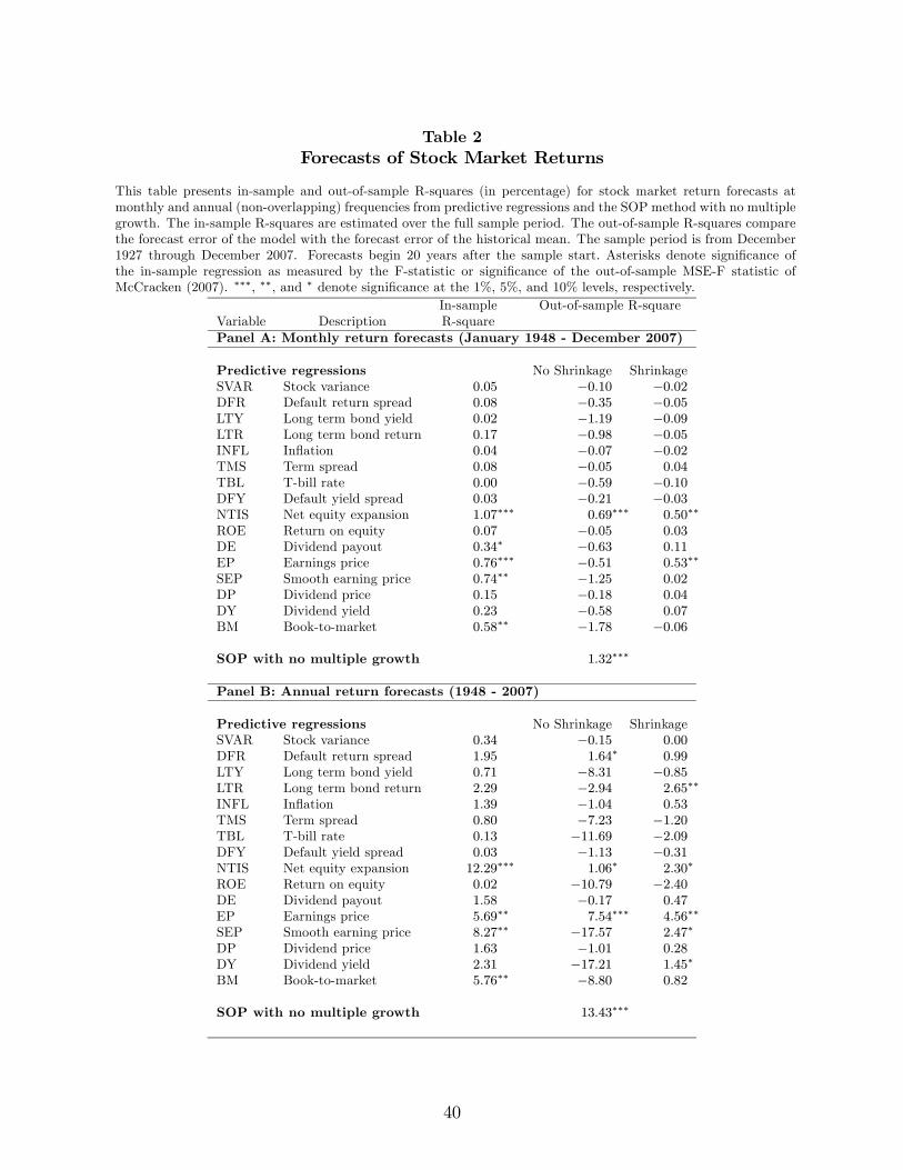
Table 2
Forecasts of Stock Market Returns
This table presents in-sample and out-of-sample R-squares (in percentage) for stock market return forecasts at
monthly and annual (non-overlapping) frequencies from predictive regressions and the SOP method with no multiple
growth. The in-sample R-squares are estimated over the full sample period. The out-of-sample R-squares compare
the forecast error of the model with the forecast error of the historical mean. The sample period is from December
1927 through December 2007. Forecasts begin 20 years after the sample start. Asterisks denote significance of
the in-sample regression as measured by the F-statistic or significance of the out-of-sample MSE-F statistic of
McCracken (2007). ∗∗∗, ∗∗, and ∗ denote significance at the 1%, 5%, and 10% levels, respectively.
In-sample Out-of-sample R-square
Variable Description R-square
Panel A: Monthly return forecasts (January 1948 - December 2007)
Predictive regressions No Shrinkage Shrinkage
SVAR Stock variance 005 −010 −002DFR Default return spread 008 −035 −005LTY Long term bond yield 002 −119 −009LTR Long term bond return 017 −098 −005INFL Inflation 004 −007 −002TMS Term spread 008 −005 004TBL T-bill rate 000 −059 −010DFY Default yield spread 003 −021 −003NTIS Net equity expansion 107∗∗∗ 069∗∗∗ 050∗∗
ROE Return on equity 007 −005 003DE Dividend payout 034∗ −063 011EP Earnings price 076∗∗∗ −051 053∗∗
SEP Smooth earning price 074∗∗ −125 002DP Dividend price 015 −018 004DY Dividend yield 023 −058 007BM Book-to-market 058∗∗ −178 −006
SOP with no multiple growth 132∗∗∗
Panel B: Annual return forecasts (1948 - 2007)
Predictive regressions No Shrinkage Shrinkage
SVAR Stock variance 034 −015 000DFR Default return spread 195 164∗ 099LTY Long term bond yield 071 −831 −085LTR Long term bond return 229 −294 265∗∗
INFL Inflation 139 −104 053TMS Term spread 080 −723 −120TBL T-bill rate 013 −1169 −209DFY Default yield spread 003 −113 −031NTIS Net equity expansion 1229∗∗∗ 106∗ 230∗
ROE Return on equity 002 −1079 −240DE Dividend payout 158 −017 047EP Earnings price 569∗∗ 754∗∗∗ 456∗∗
SEP Smooth earning price 827∗∗ −1757 247∗
DP Dividend price 163 −101 028DY Dividend yield 231 −1721 145∗
BM Book-to-market 576∗∗ −880 082
SOP with no multiple growth 1343∗∗∗
40
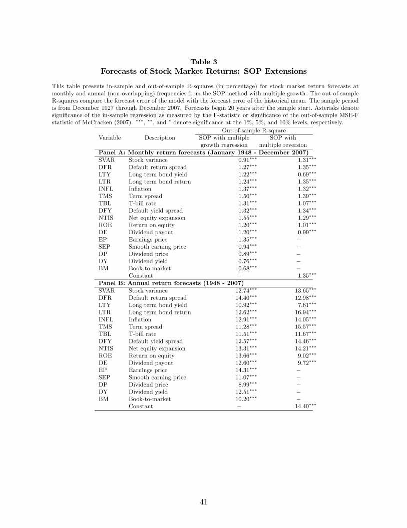
Table 3
Forecasts of Stock Market Returns: SOP Extensions
This table presents in-sample and out-of-sample R-squares (in percentage) for stock market return forecasts at
monthly and annual (non-overlapping) frequencies from the SOP method with multiple growth. The out-of-sample
R-squares compare the forecast error of the model with the forecast error of the historical mean. The sample period
is from December 1927 through December 2007. Forecasts begin 20 years after the sample start. Asterisks denote
significance of the in-sample regression as measured by the F-statistic or significance of the out-of-sample MSE-F
statistic of McCracken (2007). ∗∗∗, ∗∗, and ∗ denote significance at the 1%, 5%, and 10% levels, respectively.
Out-of-sample R-square
Variable Description SOP with multiple SOP with
growth regression multiple reversion
Panel A: Monthly return forecasts (January 1948 - December 2007)
SVAR Stock variance 091∗∗∗ 131∗∗∗
DFR Default return spread 127∗∗∗ 135∗∗∗
LTY Long term bond yield 122∗∗∗ 069∗∗∗
LTR Long term bond return 124∗∗∗ 135∗∗∗
INFL Inflation 137∗∗∗ 132∗∗∗
TMS Term spread 150∗∗∗ 139∗∗∗
TBL T-bill rate 131∗∗∗ 107∗∗∗
DFY Default yield spread 132∗∗∗ 134∗∗∗
NTIS Net equity expansion 155∗∗∗ 129∗∗∗
ROE Return on equity 120∗∗∗ 101∗∗∗
DE Dividend payout 120∗∗∗ 099∗∗∗
EP Earnings price 135∗∗∗ −SEP Smooth earning price 094∗∗∗ −DP Dividend price 089∗∗∗ −DY Dividend yield 076∗∗∗ −BM Book-to-market 068∗∗∗ −
Constant − 135∗∗∗
Panel B: Annual return forecasts (1948 - 2007)
SVAR Stock variance 1274∗∗∗ 1365∗∗∗
DFR Default return spread 1440∗∗∗ 1298∗∗∗
LTY Long term bond yield 1092∗∗∗ 761∗∗∗
LTR Long term bond return 1262∗∗∗ 1694∗∗∗
INFL Inflation 1291∗∗∗ 1405∗∗∗
TMS Term spread 1128∗∗∗ 1557∗∗∗
TBL T-bill rate 1151∗∗∗ 1167∗∗∗
DFY Default yield spread 1257∗∗∗ 1446∗∗∗
NTIS Net equity expansion 1331∗∗∗ 1421∗∗∗
ROE Return on equity 1366∗∗∗ 902∗∗∗
DE Dividend payout 1260∗∗∗ 972∗∗∗
EP Earnings price 1431∗∗∗ −SEP Smooth earning price 1107∗∗∗ −DP Dividend price 899∗∗∗ −DY Dividend yield 1251∗∗∗ −BM Book-to-market 1020∗∗∗ −
Constant − 1440∗∗∗
41

Table 4
Forecasts of Stock Market Returns: Subsamples
This table presents in-sample and out-of-sample R-squares (in percentage) for stock market return forecasts at monthly and
annual (non-overlapping) frequencies from predictive regressions and the SOP method. The in-sample R-squares are estimated
over the full sample period. The out-of-sample R-squares compare the forecast error of the model with the forecast error of
the historical mean. The sample period is from December 1927 through December 2007. Forecasts begin 20 years after the
sample start. The subsamples divide the forecast period in half. Asterisks denote significance of the in-sample regression as
measured by the F-statistic or significance of the out-of-sample MSE-F statistic of McCracken (2007). ∗∗∗, ∗∗, and ∗ denotesignificance at the 1%, 5%, and 10% levels, respectively.
In-sample Out-of-sample R-square
Variable Description R-square Predictive Predictive SOP SOP SOP
regression regression no multiple multiple multiple
(shrinkage) growth growth reg. reversion
Panel A.1: Monthly return forecasts (January 1948 - December 1976)
− − − − 180∗∗∗ − −SVAR Stock variance 000 −018 −004 − 164∗∗∗ 213∗∗∗
DFR Default return spread 001 −104 −022 − 157∗∗∗ 210∗∗∗
LTY Long term bond yield 011 −172 004 − 161∗∗∗ 093∗∗∗
LTR Long term bond return 012 −220 −034 − 142∗∗∗ 221∗∗∗
INFL Inflation 013 021∗ 008 − 219∗∗∗ 223∗∗∗
TMS Term spread 012 024∗ 010 − 206∗∗∗ 218∗∗∗
TBL T-bill rate 017 −015 009 − 190∗∗∗ 164∗∗∗
DFY Default yield spread 001 −053 −009 − 180∗∗∗ 211∗∗∗
NTIS Net equity expansion 108∗∗ 037∗ 016 − 185∗∗∗ 212∗∗∗
ROE Return on equity 001 −017 −003 − 174∗∗∗ 225∗∗∗
DE Dividend payout 047∗ −109 002 − 173∗∗∗ 216∗∗∗
EP Earnings price 107∗∗ −040 065∗∗ − 215∗∗∗ −SEP Smooth earnings price 183∗∗∗ −145 011 − 206∗∗∗ −DP Dividend price 024 029∗ 020∗ − 226∗∗∗ −DY Dividend yield 047∗ −007 033∗ − 229∗∗∗ −BM Book-to-market 162∗∗∗ 004 039∗ − 228∗∗∗ −
Constant − − − − − 214∗∗∗
Panel B.1: Annual return forecasts (1948 - 1976)
− − − − 1466∗∗∗ − −SVAR Stock variance 019 −076 −021 − 1393∗∗∗ 2154∗∗∗
DFR Default return spread 234 452∗ 166 − 1482∗∗∗ 2017∗∗∗
LTY Long term bond yield 070 −1095 −082 − 962∗∗ 1340∗∗∗
LTR Long term bond return 682∗ 964∗ 510∗∗ − 1344∗∗∗ 2518∗∗∗
INFL Inflation 149 −099 072 − 1377∗∗∗ 2218∗∗∗
TMS Term spread 191 −666 −068 − 1280∗∗∗ 2185∗∗∗
TBL T-bill rate 159 −1214 −143 − 1166∗∗ 1831∗∗∗
DFY Default yield spread 005 −164 −043 − 1456∗∗∗ 2198∗∗∗
NTIS Net equity expansion 1491∗∗∗ 065 031 − 1459∗∗∗ 2175∗∗∗
ROE Return on equity 091 −1262 −193 − 1473∗∗∗ 2282∗∗∗
DE Dividend payout 130 −023 −012 − 1309∗∗∗ 2152∗∗∗
EP Earnings price 674∗ 1414∗∗∗ 471∗ − 2177∗∗∗ −SEP Smooth earnings price 2244∗∗∗ −1042 591∗∗ − 2321∗∗∗ −DP Dividend price 293 448∗ 182 − 2102∗∗∗ −DY Dividend yield 528 −1774 434∗ − 1816∗∗∗ −BM Book-to-market 1473∗∗∗ 830∗∗∗ 441∗ − 1987∗∗∗ −
Constant − − − − − 2176∗∗∗
42
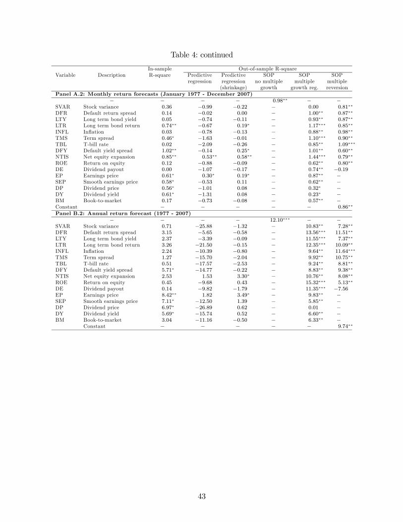
Table 4: continued
In-sample Out-of-sample R-square
Variable Description R-square Predictive Predictive SOP SOP SOP
regression regression no multiple multiple multiple
(shrinkage) growth growth reg. reversion
Panel A.2: Monthly return forecasts (January 1977 - December 2007)
− − − − 098∗∗ − −SVAR Stock variance 036 −099 −022 − 000 081∗∗
DFR Default return spread 014 −002 000 − 100∗∗ 087∗∗
LTY Long term bond yield 005 −074 −011 − 093∗∗ 087∗∗
LTR Long term bond return 074∗∗ −067 019∗ − 117∗∗∗ 085∗∗
INFL Inflation 003 −078 −013 − 088∗∗ 098∗∗
TMS Term spread 046∗ −163 −001 − 110∗∗∗ 090∗∗
TBL T-bill rate 002 −209 −026 − 085∗∗ 109∗∗∗
DFY Default yield spread 102∗∗ −014 025∗ − 101∗∗ 060∗∗
NTIS Net equity expansion 085∗∗ 053∗∗ 058∗∗ − 144∗∗∗ 079∗∗
ROE Return on equity 012 −088 −009 − 062∗∗ 080∗∗
DE Dividend payout 000 −107 −017 − 074∗∗ −019EP Earnings price 061∗ 030∗ 019∗ − 087∗∗ −SEP Smooth earnings price 058∗ −053 011 − 062∗∗ −DP Dividend price 056∗ −101 008 − 032∗ −DY Dividend yield 061∗ −131 008 − 023∗ −BM Book-to-market 017 −073 −008 − 057∗∗ −Constant − − − − − 086∗∗
Panel B.2: Annual return forecast (1977 - 2007)
− − − − 1210∗∗∗ − −SVAR Stock variance 071 −2588 −132 − 1083∗∗ 728∗∗
DFR Default return spread 315 −565 −058 − 1356∗∗∗ 1151∗∗
LTY Long term bond yield 237 −339 −009 − 1155∗∗∗ 737∗∗
LTR Long term bond return 326 −2150 −015 − 1235∗∗∗ 1009∗∗
INFL Inflation 224 −1039 −080 − 964∗∗ 1164∗∗∗
TMS Term spread 127 −1570 −204 − 992∗∗ 1075∗∗
TBL T-bill rate 051 −1757 −253 − 924∗∗ 881∗∗
DFY Default yield spread 571∗ −1477 −022 − 883∗∗ 938∗∗
NTIS Net equity expansion 253 153 330∗ − 1076∗∗ 808∗∗
ROE Return on equity 045 −968 043 − 1532∗∗∗ 513∗∗
DE Dividend payout 014 −982 −179 − 1135∗∗∗ −756EP Earnings price 842∗∗ 182 349∗ − 983∗∗ −SEP Smooth earnings price 711∗ −1250 139 − 585∗∗ −DP Dividend price 697∗ −2689 062 − 001 −DY Dividend yield 569∗ −1574 052 − 660∗∗ −BM Book-to-market 304 −1116 −050 − 633∗∗ −
Constant − − − − − 974∗∗
43

Table 5
Trading Strategies: Certainty Equivalent Gains
This table presents out-of-sample portfolio choice results at monthly and annual (non-overlapping) frequencies from
predictive regressions and the SOP method. The numbers are the certainty equivalent gains (in percentage) of a
trading strategy timing the market with different return forecasts relative to timing the market with the historical
mean return. The certainty equivalent return is −
22() with a risk-aversion coefficient of = 2. All numbers
are annualized (monthly certainty equivalent gains are multiplied by 12). The sample period is from December
1927 through December 2007. Forecasts begin 20 years after the sample start.
Variable Description Predictive Predictive SOP SOP SOP
regression regression no multiple multiple multiple
(shrinkage) growth growth reg. reversion
Panel A: Monthly return forecasts (January 1948 - December 2007)
− − − 179 − −SVAR Stock variance −004 000 − 097 161DFR Default return spread −026 −004 − 175 172LTY Long term bond yield −156 −029 − 176 126LTR Long term bond return −025 010 − 192 168INFL Inflation −007 −002 − 186 165TMS Term spread 041 018 − 213 172TBL T-bill rate −086 −018 − 175 138DFY Default yield spread −019 −005 − 153 165NTIS Net equity expansion 214 094 − 233 159ROE Return on equity 028 017 − 169 118DE Dividend payout 140 057 − 156 094EP Earnings price 020 035 − 169 −SEP Smooth earnings price −115 −041 − 073 −DP Dividend price −084 −026 − 062 −DY Dividend yield −121 −033 − 045 −BM Book-to-market −258 −052 − 049 −
Constant − − − − 169Panel B: Annual return forecasts (1948 - 2007)
− − − 182 − −SVAR Stock variance 012 004 − 166 154DFR Default return spread 048 020 − 207 151LTY Long term bond yield −105 −019 − 175 092LTR Long term bond return 148 066 − 188 195INFL Inflation −008 008 − 173 147TMS Term spread −058 −008 − 152 184TBL T-bill rate −148 −031 − 169 125DFY Default yield spread −001 −001 − 158 165NTIS Net equity expansion 125 054 − 189 164ROE Return on equity −109 −028 − 204 078DE Dividend payout 060 024 − 191 074EP Earnings price 058 034 − 166 −SEP Smooth earnings price −139 −014 − 088 −DP Dividend price −071 −022 − 054 −DY Dividend yield −204 −016 − 141 −BM Book-to-market −153 −027 − 097 −
Constant − − − − 167
44

Table 6
Trading Strategies: Sharpe Ratio Gains
This table presents out-of-sample portfolio choice results at monthly and annual (non-overlapping) frequencies from
predictive regressions and the SOP method. The numbers are the change in Sharpe ratio of a trading strategy
timing the market with different return forecasts relative to timing the market with the historical mean return. All
numbers are annualized. The sample period is from December 1927 through December 2007. Forecasts begin 20
years after the sample start.
Variable Description Predictive Predictive SOP SOP SOP
regression regression no multiple multiple multiple
(shrinkage) growth growth reg. reversion
Panel A: Monthly return forecasts (January 1948 - December 2007)
− − − 031 − −SVAR Stock variance 000 000 − 012 022DFR Default return spread −006 −001 − 030 024LTY Long term bond yield −025 −006 − 029 009LTR Long term bond return −012 −002 − 023 024INFL Inflation −004 −001 − 031 019TMS Term spread −005 −002 − 028 023TBL T-bill rate −018 −004 − 032 016DFY Default yield spread −002 000 − 033 024NTIS Net equity expansion 004 006 − 028 024ROE Return on equity −006 −002 − 027 012DE Dividend payout −002 000 − 032 014EP Earnings price −009 030 − 023 −SEP Smooth earnings price −021 012 − 012 −DP Dividend price 011 008 − 014 −DY Dividend yield −013 015 − 007 −BM Book-to-market −034 004 − 001 −
Constant − − − − 024Panel B: Annual return forecasts (1948 - 2007)
− − − 022 − −SVAR Stock variance 001 000 − 023 011DFR Default return spread 003 002 − 023 012LTY Long term bond yield −014 −003 − 019 002LTR Long term bond return 008 006 − 023 015INFL Inflation 001 002 − 021 009TMS Term spread −010 −002 − 018 015TBL T-bill rate −019 −004 − 019 008DFY Default yield spread −001 −001 − 024 013NTIS Net equity expansion 005 004 − 022 012ROE Return on equity −015 −004 − 016 003DE Dividend payout 000 000 − 021 004EP Earnings price 005 015 − 012 −SEP Smooth earnings price −015 007 − 006 −DP Dividend price −002 002 − 004 −DY Dividend yield −021 007 − 020 −BM Book-to-market −019 003 − 009 −
Constant − − − − 013
45

Table 7
Forecasts of Stock Market Returns: International Evidence
This table presents in-sample and out-of-sample R-squares (in percentage) for stock market return forecasts at annual (non-overlapping) frequency in the U.K.
(Panel A), Japan (Panel B), and the U.S. (Panel C) from predictive regressions and the SOP method. The in-sample R-squares are estimated over the full sample
period. The out-of-sample R-squares compare the forecast error of the model with the forecast error of the historical mean. The sample period is from 1950 or
1960 through 2007. Forecasts begin 20 years after the sample start. Asterisks denote significance of the in-sample regression as measured by the F-statistic or
significance of the out-of-sample MSE-F statistic of McCracken (2007). ∗∗∗, ∗∗, and ∗ denote significance at the 1%, 5%, and 10% levels, respectively.
In-sample Out-of-sample R-square
Variable Description Forecast R-square Predictive Predictive SOP SOP SOP
start regression regression no multiple multiple multiple
(shrinkage) growth growth reg. reversion
Panel A: U.K. annual return forecasts
− 1970 − − − 1073∗∗∗ − −LTY Long term bond yield 1970 529∗ −4754 −561 − 416∗∗ 1127∗∗∗
TMS Term spread 1970 310 −1471 −113 − 926∗∗ 1160∗∗∗
TBL T-bill rate 1970 147 −2087 −307 − 639∗∗ 1151∗∗∗
DY Dividend yield 1970 1197∗∗∗ −919 507∗∗ − 1328∗∗∗ 1078∗∗∗
Constant 1970 − − − − − 1175∗∗∗
Panel B: Japan annual return forecasts
− 1970 − − − 1214∗∗∗ − −LTY Long term bond yield 1970 169 −1101 −186 − 1211∗∗∗ 1187∗∗∗
TMS Term spread 1980 036 −546 −089 − 575∗∗ 582∗∗
TBL T-bill rate 1980 176 −757 −062 − 514∗ 562∗∗
DY Dividend yield 1970 1524∗∗∗ 312∗ 663∗∗ − 1025∗∗∗ 1199∗∗∗
Constant 1970 − − − − − 1191∗∗∗
Panel C: U.S. annual return forecasts
− 1970 − − − 775∗∗ − −LTY Long term bond yield 1970 017 −2073 −151 − 447∗∗ 312∗
TMS Term spread 1970 111 −1205 −099 − 824∗∗ 550∗∗
TBL T-bill rate 1970 003 −2118 −200 − 506∗∗ 340∗
DY Dividend yield 1970 795∗∗ 096 268∗ − 664∗∗ 573∗∗
Constant 1970 − − − − − 592∗∗
46

Table 8
Forecasts of Stock Market Returns: Analyst Earnings Forecasts
This table presents in-sample and out-of-sample R-squares (in percentage) for stock market return forecasts at monthly frequency from predictive regressions and the SOP
method. The in-sample R-squares are estimated over the full sample period. The out-of-sample R-squares compare the forecast error of the model with the forecast error of
the historical mean. The SOP method uses alternatively analyst earnings forecasts and historical earnings to calculate and . The sample period is from January 1982
through December 2007. Forecasts begin 5 years after the sample start. Asterisks denote significance of the in-sample regression as measured by the F-statistic or significance
of the out-of-sample MSE-F statistic of McCracken (2007). ∗∗∗, ∗∗, and ∗ denote significance at the 1%, 5%, and 10% levels, respectively.
In-sample Out-of-sample R-square
Variable Description R-square Predictive Predictive SOP - Analyst forecasts SOP - Historical data
regression regression no multiple multiple multiple no multiple multiple multiple
(shrinkage) growth growth reg. reversion growth growth reversion
Monthly return forecasts (January 1987 - December 2007)
- − − − 232∗∗∗ − − 362∗∗∗ − −SVAR Stock variance 088 −297 −017 − 226∗∗∗ 215∗∗∗ − 281∗∗∗ 359∗∗∗
DFR Default return spread 060 −220 −014 − 220∗∗∗ 219∗∗∗ − 351∗∗∗ 362∗∗∗
LTY Long term bond yield 026 −067 −002 − 225∗∗∗ 310∗∗∗ − 352∗∗∗ 466∗∗∗
LTR Long term bond return 026 −045 −001 − 226∗∗∗ 217∗∗∗ − 360∗∗∗ 358∗∗∗
INFL Inflation 004 −076 −006 − 222∗∗∗ 213∗∗∗ − 354∗∗∗ 362∗∗∗
TMS Term spread 001 −200 −015 − 215∗∗∗ 207∗∗∗ − 322∗∗∗ 359∗∗∗
TBL T-bill rate 029 −118 −003 − 219∗∗∗ 260∗∗∗ − 337∗∗∗ 423∗∗∗
DFY Default yield spread 051 −049 004 − 212∗∗∗ 231∗∗∗ − 334∗∗∗ 350∗∗∗
NTIS Net equity expansion 066 −123 006 − 201∗∗∗ 237∗∗∗ − 297∗∗∗ 362∗∗∗
ROE Return on equity 002 −184 −010 − 197∗∗∗ 223∗∗∗ − 317∗∗∗ 354∗∗∗
DE Dividend payout 002 −179 −012 − 226∗∗∗ 170∗∗∗ − 359∗∗∗ 313∗∗∗
EP Earnings price 268∗∗∗ 178∗∗∗ 056∗ − 239∗∗∗ − − 361∗∗∗ −SEP Smooth earnings price 125∗∗ −022 019 − 213∗∗∗ − − 339∗∗∗ −DP Dividend price 174∗∗ 000 029∗ − 208∗∗∗ − − 329∗∗∗ −DY Dividend yield 174∗∗ −023 028∗ − 207∗∗∗ − − 325∗∗∗ −BM Book-to-market 102∗ 014 014 − 216∗∗∗ − − 339∗∗∗ −
Constant − − − − − 217∗∗∗ − − 361∗∗∗
47
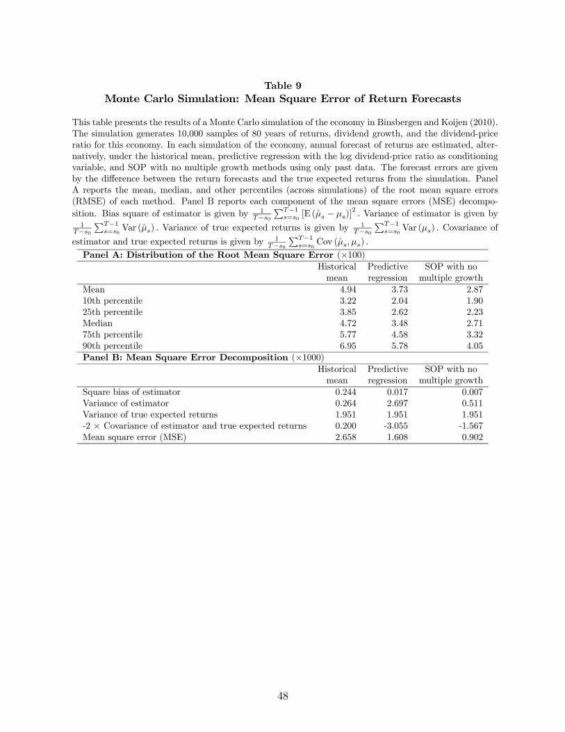
Table 9
Monte Carlo Simulation: Mean Square Error of Return Forecasts
This table presents the results of a Monte Carlo simulation of the economy in Binsbergen and Koijen (2010).
The simulation generates 10,000 samples of 80 years of returns, dividend growth, and the dividend-price
ratio for this economy. In each simulation of the economy, annual forecast of returns are estimated, alter-
natively, under the historical mean, predictive regression with the log dividend-price ratio as conditioning
variable, and SOP with no multiple growth methods using only past data. The forecast errors are given
by the difference between the return forecasts and the true expected returns from the simulation. Panel
A reports the mean, median, and other percentiles (across simulations) of the root mean square errors
(RMSE) of each method. Panel B reports each component of the mean square errors (MSE) decompo-
sition. Bias square of estimator is given by 1−0
P−1=0
[E ( − )]2 Variance of estimator is given by
1−0
P−1=0
Var () Variance of true expected returns is given by1
−0P−1
=0Var () Covariance of
estimator and true expected returns is given by 1−0
P−1=0
Cov ( )
Panel A: Distribution of the Root Mean Square Error (×100)Historical Predictive SOP with no
mean regression multiple growth
Mean 4.94 3.73 2.87
10th percentile 3.22 2.04 1.90
25th percentile 3.85 2.62 2.23
Median 4.72 3.48 2.71
75th percentile 5.77 4.58 3.32
90th percentile 6.95 5.78 4.05
Panel B: Mean Square Error Decomposition (×1000)Historical Predictive SOP with no
mean regression multiple growth
Square bias of estimator 0.244 0.017 0.007
Variance of estimator 0.264 2.697 0.511
Variance of true expected returns 1.951 1.951 1.951
-2 × Covariance of estimator and true expected returns 0.200 -3.055 -1.567
Mean square error (MSE) 2.658 1.608 0.902
48

Figure 1. Cumulative Realized Stock Market ComponentsThis figure shows of annual realized price-earnings ratio growth (), earnings growth (), dividend price(), and stock market return () index (base year is 1947 = 1).
An
nu
al c
um
ula
tive
re
turn
ind
ex
1947 1951 1955 1959 1963 1967 1971 1975 1979 1983 1987 1991 1995 1999 2003 20070
1
2
3
4
5
6
7
8gm
ge
dp
r
49
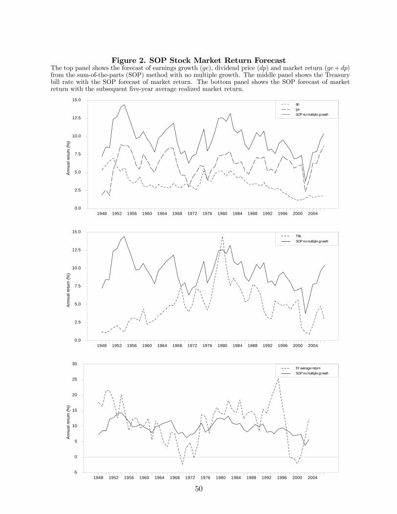
Figure 2. SOP Stock Market Return ForecastThe top panel shows the forecast of earnings growth (), dividend price () and market return (+ )from the sum-of-the-parts (SOP) method with no multiple growth. The middle panel shows the Treasurybill rate with the SOP forecast of market return. The bottom panel shows the SOP forecast of marketreturn with the subsequent five-year average realized market return.
An
nu
al r
etu
rn (
%)
1948 1952 1956 1960 1964 1968 1972 1976 1980 1984 1988 1992 1996 2000 20040.0
2.5
5.0
7.5
10.0
12.5
15.0dp
ge
SOP no multiple growth
An
nu
al r
etu
rn (
%)
1948 1952 1956 1960 1964 1968 1972 1976 1980 1984 1988 1992 1996 2000 20040.0
2.5
5.0
7.5
10.0
12.5
15.0TBL
SOP no multiple growth
An
nu
al r
etu
rn (
%)
1948 1952 1956 1960 1964 1968 1972 1976 1980 1984 1988 1992 1996 2000 2004-5
0
5
10
15
20
25
305Y average return
SOP no multiple growth
50

Figure 3. Forecast of Stock Market Return - Alternative MethodsThese figures show the forecast of market return from the historical mean, predictive regressions with DP,TMS and TBL as predictors, and sum-of-the-parts method (SOP) with no multiple growth.
DP
An
nu
al r
etu
rn (
%)
1948 1952 1956 1960 1964 1968 1972 1976 1980 1984 1988 1992 1996 2000 2004-5.0
-2.5
0.0
2.5
5.0
7.5
10.0
12.5
15.0historical mean
predictive regression
SOP no multiple growth
TMS
An
nu
al r
etu
rn (
%)
1948 1952 1956 1960 1964 1968 1972 1976 1980 1984 1988 1992 1996 2000 2004-5.0
-2.5
0.0
2.5
5.0
7.5
10.0
12.5
15.0historical mean
predictive regression
SOP no multiple growth
TBL
An
nu
al r
etu
rn (
%)
1948 1952 1956 1960 1964 1968 1972 1976 1980 1984 1988 1992 1996 2000 2004-5.0
-2.5
0.0
2.5
5.0
7.5
10.0
12.5
15.0historical mean
predictive regression
SOP no multiple growth
51

Figure 4. Cumulative R-squareThese figures show out-of-sample cumulative R-square up to each year from predictive regressions with DP,TMS and TBL as predictors, and the sum-of-the-parts method (SOP) with no multiple growth relative tothe historical mean.
DP
Cu
mu
lativ
e R
-sq
ua
red
diff
ere
nce
(%
)
1948 1952 1956 1960 1964 1968 1972 1976 1980 1984 1988 1992 1996 2000 2004-75
-50
-25
0
25
50
75predictive regression
SOP no multiple growth
TMS
Cu
mu
lativ
e R
-sq
ua
red
diff
ere
nce
(%
)
1948 1952 1956 1960 1964 1968 1972 1976 1980 1984 1988 1992 1996 2000 2004-75
-50
-25
0
25
50
75predictive regression
SOP no multiple growth
TBL
Cu
mu
lativ
e R
-sq
ua
red
diff
ere
nce
(%
)
1948 1952 1956 1960 1964 1968 1972 1976 1980 1984 1988 1992 1996 2000 2004-75
-50
-25
0
25
50
75predictive regression
SOP no multiple growth
52
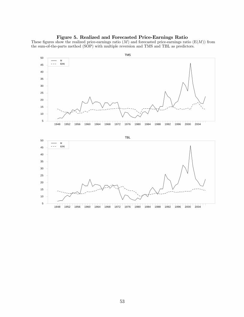
Figure 5. Realized and Forecasted Price-Earnings RatioThese figures show the realized price-earnings ratio () and forecasted price-earnings ratio (E()) fromthe sum-of-the-parts method (SOP) with multiple reversion and TMS and TBL as predictors.
TMS
1948 1952 1956 1960 1964 1968 1972 1976 1980 1984 1988 1992 1996 2000 20045
10
15
20
25
30
35
40
45
50M
E(M)
TBL
1948 1952 1956 1960 1964 1968 1972 1976 1980 1984 1988 1992 1996 2000 20045
10
15
20
25
30
35
40
45
50M
E(M)
53
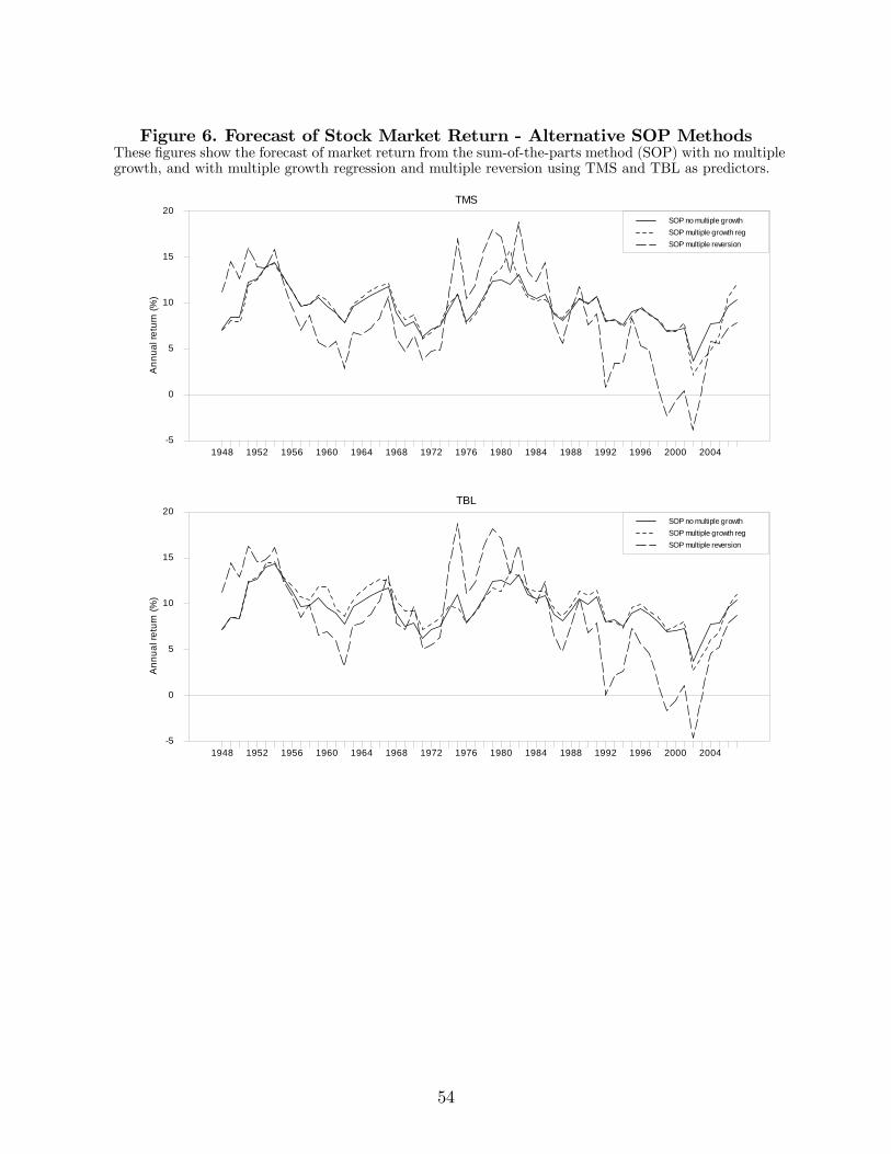
Figure 6. Forecast of Stock Market Return - Alternative SOP MethodsThese figures show the forecast of market return from the sum-of-the-parts method (SOP) with no multiplegrowth, and with multiple growth regression and multiple reversion using TMS and TBL as predictors.
TMS
An
nu
al r
etu
rn (
%)
1948 1952 1956 1960 1964 1968 1972 1976 1980 1984 1988 1992 1996 2000 2004-5
0
5
10
15
20SOP no multiple growth
SOP multiple growth reg
SOP multiple reversion
TBL
An
nu
al r
etu
rn (
%)
1948 1952 1956 1960 1964 1968 1972 1976 1980 1984 1988 1992 1996 2000 2004-5
0
5
10
15
20SOP no multiple growth
SOP multiple growth reg
SOP multiple reversion
54
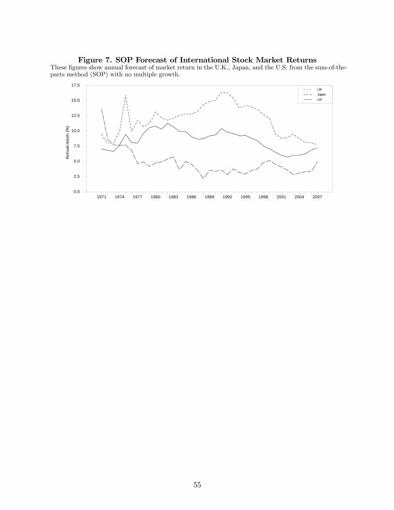
Figure 7. SOP Forecast of International Stock Market ReturnsThese figures show annual forecast of market return in the U.K., Japan, and the U.S. from the sum-of-the-parts method (SOP) with no multiple growth.
An
nu
al r
etu
rn (
%)
1971 1974 1977 1980 1983 1986 1989 1992 1995 1998 2001 2004 20070.0
2.5
5.0
7.5
10.0
12.5
15.0
17.5UK
Japan
US
55

Figure 8. Monte Carlo SimulationThis figure plots expected return estimates against true expected returns from a Monte Carlo simulationof the economy in Binsbergen and Koijen (2010). The simulation generates 10,000 samples of 80 years ofreturns, dividend growth, and the dividend-price ratio for this economy. In each simulation of the economy,annual expected returns are estimated with past data using the historical mean, predictive regression withthe log dividend-price ratio as conditioning variable, and the SOP method with no multiple growth. Thesolid line is a 45 degree line.
56


![Time Series Analysis on Stock Returns - WordPress.com · of Markowitz (1959) [2]. However, model using a market factor does a poor job at forecasting future returns. One needs to](https://img.pdfslide.us/doc/110x75/5f7ffb5940c70070752eea33/time-series-analysis-on-stock-returns-of-markowitz-1959-2-however-model.jpg)