PREDICTIVE LOSS RATIO MODELING WITH … loss ratio modeling with credit scores, ... build sample ... 61 commercial auto

PREDICTIVE LOSS RATIO

MODELING WITH CREDIT SCORES, FOR INSURANCE PURPOSES

Major Qualifying Project submitted to the faculty of Worcester Polytechnic Institute in partial

fulfillment of the requirements for the Degree of Bachelor of Science in Actuarial Mathematics

4/26/2012 Jon Abraham, Advisor Isin Ozaksoy, Liaison

Corey Alfieri Taylor Ketterer

Ricardo Obasare Kyaw Thiha

1

TABLE OF CONTENTS

ACKNOWLEDGEMENTS ................................................................................................................ 3

EXECUTIVE SUMMARY .................................................................................................................. 4

INTRODUCTION ............................................................................................................................... 6

BACKGROUND ................................................................................................................................. 9

HANOVER INSURANCE BACKGROUND .............................................................................................. 9

PREDICTIVE MODELING .................................................................................................................... 10

CREDIT SCORE USAGE IN INSURANCE .............................................................................................. 11

GOVERNMENT REGULATORY ENVIRONMENT ................................................................................ 14

MULTIVARIATE MODELS ................................................................................................................... 14

GENERALIZED LINEAR MODELS ......................................................................................................... 14

DECISION TREE ANALYSIS ................................................................................................................... 16

MULTIVARIATE ADAPTIVE REGRESSION SPLINES (MARS) ............................................................... 16

MODEL DISTRIBUTION TYPE: TWEEDIE DISTRIBUTION ................................................................ 17

METHODOLOGY ............................................................................................................................ 19

ANALYSIS AND DISCUSSION ................................................................................................... 25

1. FINANCIAL STABILITY LOSS RATIO RELATIVITIES ................................................................. 26

2. POLICY TYPE LOSS RATIO RELATIVITIES.................................................................................. 27

3. BUSINESS TYPE LOSS RATIO RELATIVITIES ............................................................................. 28

4. MARKET SEGMENT LOSS RATIO RELATIVITIES ...................................................................... 29

5. FLEET SIZE LOSS RATIO RELATIVITIES ..................................................................................... 30

6. POLICY EFFECTIVE AGE LOSS RATIO RELATIVITIES ............................................................... 31

7. C-POINTS LOSS RATIO RELATIVITIES ....................................................................................... 32

8. F-POINTS LOSS RATIO RELATIVITIES ....................................................................................... 33

CONCLUSIONS AND RECOMMENDATIONS ....................................................................... 34

APPENDIX A: GLOSSARY............................................................................................................. 37

APPENDIX B: PROCESS OVERVIEW CHART ......................................................................... 39

APPENDIX C: COMMERCIAL AUTO CHARTS ...................................................................... 40

FINANCIAL STABILITY LIFT CHARTS ................................................................................................ 40

BUILD SAMPLE ..................................................................................................................................... 40

VALIDATION SAMPLE .......................................................................................................................... 40

POLICY TYPE LIFT CHARTS ................................................................................................................ 41

BUILD SAMPLE ..................................................................................................................................... 41


2

BUSINESS TYPE LIFT CHARTS ............................................................................................................ 42

BUILD SAMPLE ..................................................................................................................................... 42


MARKET SEGMENT LIFT CHARTS ..................................................................................................... 43

BUILD SAMPLE ..................................................................................................................................... 43


FLEET SIZE LIFT CHARTS ................................................................................................................... 44

BUILD SAMPLE ..................................................................................................................................... 44


POLICY EFFECTIVE AGE LIFT CHARTS .............................................................................................. 45

BUILD SAMPLE ..................................................................................................................................... 45


C-POINTS LIFT CHARTS ..................................................................................................................... 46

BUILD SAMPLE ..................................................................................................................................... 46


F-POINTS LIFT CHARTS ...................................................................................................................... 47

BUILD SAMPLE ..................................................................................................................................... 47


FINANCIAL STABILITY LIFT CHARTS ................................................................................................ 48

BUILD SAMPLE ..................................................................................................................................... 48


APPENDIX D: BUSINESS OWNER’S POLICY CHARTS........................................................ 49

APPENDIX E: MODEL COEFFICIENTS ..................................................................................... 59

COMMERCIAL AUTO .......................................................................................................................... 59

BUSINESS OWNER’S POLICY .............................................................................................................. 60

APPENDIX F: CODE ........................................................................................................................ 61

COMMERCIAL AUTO .......................................................................................................................... 61

DATA PREPARATION ........................................................................................................................... 61

FITTING ................................................................................................................................................. 61

LIFT CHARTS ........................................................................................................................................ 62

BUSINESS OWNERS POLICY ............................................................................................................... 63

REFERENCES .................................................................................................................................... 64

3

ACKNOWLEDGEMENTS

Our team would like to first thank our sponsor The Hanover Insurance Group and

the entire team working there; without them, the idea for this project would not have

existed. We would especially like to thank Isin Osaksoy and Marc Cournoyer for all their

guidance and support throughout the duration of our project. Additionally, we would like

to thank the Commercial Auto team; Jaris Wicklund and Andrew Evans; as well as the

Business Owners Policy team; Jonathon Blake, Alyssa Potter and Chen Li. We are very

grateful to these individuals for assisting us in shaping the direction of our project and for

their willingness to share their knowledge and expertise on the insurance industry. Finally,

we would like to thank Professor Jon Abraham for constantly pushing us to do our best and

for his continued support when we faced challenges along the way. We also extend our

thanks to everyone at Worcester Polytechnic Institute (WPI) and The Hanover Insurance

Group that made this experience possible.

4

EXECUTIVE SUMMARY

Hanover Insurance Group is a publicly traded property and casualty insurance

company that is based in Worcester, Massachusetts. They provide their customers with a

wide range of insurance products for both personal and commercial business lines. In recent

times, credit scores have gained widespread popularity within the insurance industry,

especially in the underwriting and pricing, due to its powerful predictive value. Hanover

Insurance commissioned a team of four students from Worcester Polytechnic Institute (WPI)

to design a statistical model that incorporates the credit score of each policy to better predict

the future level of risk associated with this policy.

The goal of this project was to create a loss ratio model that would improve the

predictive ability of the current Hanover premium model through implementation of credit

scores. This would enable Hanover to benefit from more informed underwriting and pricing

techniques, greater competitive advantage in commercial insurance lines of business and

most importantly, more robust underwriting profit. Steps included:

Conducting weekly meetings with the project advisors to interpret and

analyze weekly results.

Utilizing statistical software such as Microsoft Excel, SAS and R to analyze

and model data.

Developing graphical charts of variables that are statistically significant to the

model, in order to determine model accuracy.

Recommendations for improving current underwriting and pricing

techniques.

The methodology consists of 3 primary steps. Our first step was to analyze the

current techniques that Hanover employs in pricing and underwriting. This was done in

order to identify the risk factors considered and to develop a solution to uniquely address

5

their business issue. Our next step was to familiarize ourselves with the data set to detect

data quality issues and prepare the data for modeling. It is vital that the data be cleaned

before usage as our model’s predictive ability depends primarily on the quality of the input

data. We noted any outliers, missing data, and inconsistent or invalid data points and

identified statistically significant variables to be used in the model. Once we completed our

data preparation we proceeded with the final step, data modeling. We used a generalized

linear model with Tweedie distribution to predict the loss ratios of the policies, and used

trial and error methods to test model accuracy. Once we were satisfied with the model, we

analyzed the results to develop appropriate risk categories to differentiate customers based

on the level of risk indicated by their predicted loss ratio.

The purpose of this project was to improve Hanover’s underwriting and pricing

techniques through the implementation of credit scores. We believe that Hanover’s usage of

these credit scores combined with additional company specific data, will be a powerful tool

in predicting incurred loss ratio of a policy. Incorporating these credit scores will ensure that

Hanover’s underwriting and pricing techniques are competitive and more advanced than

similar companies within commercial insurance. Hanover’s ability to better differentiate the

risk types of their customers will ultimately improve their underwriting profit by ensuring

that they do not underwrite policies with excessively high risk.

6

INTRODUCTION

The relatively recent integration of credit score information since the late 20th

Century has significantly impacted the insurance industry; however its usage has resulted

in some level of controversy (Wu & Guszcz, 2003). A credit score is a numeric value

developed using statistical methods used to represent a customer’s level of credit worthiness

or ability to repay financial obligations. In insurance, credit scores have been used with

additional variables (driver record, type of vehicle, location of vehicle, etc.) to establish

relationships between individual responsibility and probability of a loss in the future. The

underlying assumption here is that customers who are more responsible in managing

personal finances will also be prudent in management of other aspects of their life. These

traits would lead insurance underwriters to believe that customers with a respectable credit

score will be low risk customers, hence making them desirable (Hartwig & Wilkinson, 2003,

Wu & Guszczs, 2003). If an insurance company can better classify low and high risk

customers from a pool of applicants, it can prevent them from taking on risky customers

who will have more claims and cause the company to make more payouts in the future.

Therefore more and more companies in the insurance industry have begun to harness the

predictive value of credit information.

In spite of this widespread usage, there have been several concerns raised over the

extent to which credit scores are an accurate predictive measure. Credit scores are generated

using a combination of past credit behavior of a consumer; therefore there is an issue as to

whether its usage can be used to conclusively represent their behavior in the future. Several

studies have, however, indicated that a relationship does exist between credit scores and

loss frequency. Furthermore, the inclusion of credit scores in combination with other

variables increases the accuracy. Many consumers have challenged the link between credit

scores and customer creditworthiness since a poor credit score can put them at a significant

7

disadvantage when seeking to purchase insurance. As a result of this the government has

placed restrictions and regulations on the manner in which insurance companies can use

credit information. Nonetheless, its continued usage attests to the fact that there is valuable

information that can be gained by using credit information, which will ultimately serve to

improve the financial position of a business (Hartwig & Wilkinson, 2003) (Wu & Guszcz,

2003) (Hanover Insurance Group, 2011).

The Hanover Insurance Group is a publicly traded property and casualty insurance

provider that is looking to utilize consumer credit information to improve underwriting

profit. Headquartered in Worcester, Massachusetts, Hanover focuses on providing

comprehensive insurance products to consumers in personal and commercial business lines.

Their core commercial business segments can be further broken down into commercial auto

insurance, commercial property and liability insurance, worker’s compensation insurance

and other forms of specialized insurance packages (Hanover Insurance Group, 2011).

Within the insurance industry, great emphasis is placed on developing techniques that allow

for more accurate modeling and prediction of risk. As business trends have developed, there

has been a noticeable shift to the inclusion of credit score data as a predictive measure of the

likelihood of losses associated with a customer account. Innovative implementation of a

credit score variable would allow Hanover to enhance their current pricing and

underwriting mechanisms giving them a competitive advantage. This directly influences

Hanover’s long-term profitability and market control and as a result has a key business

value to the firm. The business issue is therefore how the implementation of credit

information can improve the predictive ability of the current Hanover premium model for

the commercial lines of business.

This paper will outline the details surrounding the business issue facing the Hanover

Insurance Group and the development of the solution. We will discuss the initial appearance

of credit information in the insurance industry and how it has been used in predictive

8

modeling. Afterwards, we will indicate typical statistical models that have been used to

conduct predictive analysis. From there, we will outline specific project goals and objectives

and the approach that was taken to achieve them. Following this, we will display the results

of the model, highlighting key points and trends and analyzing the significance that the

model results have for the Hanover Insurance Group. At this stage, it will be necessary to

understand the implications of implementing this model and additional future concerns that

may affect the manner in which business is conducted at the Hanover Insurance Group.

9

BACKGROUND

Hanover Insurance Background

The Hanover Insurance Group is a property and casualty insurance company based

in Worcester, Massachusetts. They have over four thousand employees and offer a wide

range of products spanning personal and commercial lines of business. In addition, they are

a holding company for a group of insurers, offering property and casualty products and

services through a group of independent agents.

Within personal lines, Hanover offers home insurance, with four levels of coverage

from basic to select premium. Basic coverage offers replacement benefits for most common

causes of loss. In addition, it insures other structures such as sheds and garages, covers some

personal belongings, handles liability claims, and offers medical payments to non-household

members injured on the property. Each additional policy offers more coverage in addition to

the basic coverage. Hanover also offers personal auto insurance, which offers various

liability limits in addition to comprehensive and collision options, roadside assistance,

transportation expense, medical payments and personal injury protection, and value-added

endorsements. For personal insurance customers who already have home or auto insurance,

Hanover offers personal add-ons. The add-on called “Toys” covers recreational vehicles,

watercraft insurance, and account extras. Umbrella Coverage provides additional coverage

on top of the original policy, the Identity Integrity Program protects against identity theft,

and valuables insurance is also offered.

Hanover offers both small business insurance and midsize business insurance. For

small business insurance, there is standard insurance that includes Business Owners Policy

for businesses that fit specific criteria. They also offer Commercial Package Policy for the

small businesses that do not fit the criteria for a Business Owners Policy. Hanover also offers

workers’ compensation, commercial auto, and commercial umbrella policies. In addition,

10

they have special coverage and policies for small technology businesses. Hanover offers

similar policies for midsize businesses as they do for small businesses. In addition, they offer

inland marine policies, policies for marinas, jewelers’ block, and performance and surety

bonds. They also offer special policies for schools, human services, chauffeured

transportation, document management, moving and storage, religious institutions, specialty

industrial, sports and fitness, and investment management.

Predictive Modeling

Predictive modeling is an analytical method used to create statistical models that

predict future behavior or results. It is a form of data-mining that uses advanced statistical

modeling techniques to forecast probabilities and trends (Mosley, 2005). For example, a

company can use predictive modeling to identify insurance risks, which can lead to

improved underwriting, pricing and marketing decisions. For many insurance companies,

predictive modeling plays an important role in pricing techniques since it can help them

differentiate low or high risk customers based on several characteristics and, most

importantly, give them a price optimization strategy.

In recent times, predictive modeling has gained popularity and has been heavily

utilized by property and casualty insurance companies in personal lines because it gives

them a competitive advantage. Insurers believe that predictive modeling can significantly

help their rating plans by identifying mispriced risks thus increasing profitability (Mosley,

2005). By identifying new rating variables or new relationships between existing variables,

predictive modeling can find different ways to segment risks. One such method of

segmenting risk is through the inclusion of a customer’s credit history. Today, most

companies have used credit score information in predictive analysis because they have

identified a relationship between customer credit scores and likelihood of future loss. In

addition, several companies have realized the accuracy of using multivariate analyses in

11

conjunction with credit information. Even for small to medium sized companies, a custom

insurance score can greatly improve the results of current underwriting and pricing

techniques. Therefore, the usage of credit scores as a predictor of losses in commercial lines

will yield more accurate results.

There are three main stages involved in predictive modeling. Typically, identifying

the issues a company wants the model to solve is the first stage. Collecting the appropriate

data that would be needed to solve these issues is the second stage, and finally, developing

the model that best fits the data and analyzing the results are the third stage (Mosley, 2005).

The types of predictive modeling analysis methods that have received widespread attention

are the Generalized Linear Modeling (GLM), Decision Tree Analysis and Multivariate

Adaptive Regression Splines (MARS). A discussion of these modeling techniques will be

done at the end of the section.

Credit score usage in Insurance

There are several risk factors that are used by insurance companies to evaluate the

risk of customers in order to assign a proper individual premium to each. Competition

continuously forces companies to find new and more accurate factors to add to their pricing

strategies, thus ensuring more competitive pricing. In the 1980’s through the early 1990’s,

insurance companies first began to formally use elements associated with credit such as

bankruptcy history in premium pricing (Federal Trade Commission, 2007). Beginning in the

1990’s, alternative credit scores were developed and made commercially available. As the

years went on, new technology allowed for a wide range of differentiated scores to be

developed using new modeling techniques (Oscherwitz & Reemts, 2011). In 1993, Fair Isaac

Corporation developed the first credit-based insurance score. This and competing insurance

scores were developed to reflect the predicted risk for an insurance loss based on a

customer’s credit report. Since then, a number of companies have developed their own

12

credit-based insurance scores for many different insurance markets (Federal Trade

Commission, 2007). In addition, the wide availability of these scores and the increasing use

of computers and database software allowed companies to better model this credit data to

develop more practical applications of insurance scores. In fact, it was found that credit-

based insurance scores were a reliable and successful predictor of risk. Experian, a major

credit score company, found that credit scores are successfully indicative of loss 60-80% of

the time (Krickus, 2011). Today the 15 largest personal auto insurers use credit scores for

premium pricing (Federal Trade Commission, 2007).

Despite the wide acceptance of credit scores in the insurance industry, consumers

have been reluctant to accept their use. In 2001 and 2002 a number of lawsuits were filed

against GEICO and Safeco claiming they violated the Fair Credit Reporting Act, which

“requires notice to any consumer who is subjected to adverse action … based in whole or in

part on any consumer [credit] report” (Allen, Perry, Reynolds, & Long, 2008). The lawsuits

suggested that insurance companies were required to inform customers whenever their

credit history was used to negatively affect their premiums within personal auto insurance.

Eventually the Supreme Court considered the case and the issue became public. The

Supreme Court ruled “the insurance industry, under the Fair Credit Reporting Act, must

notify customers that it is charging higher insurance rates only when the higher rate is based

on a low credit score. Companies aren’t in violation of the law, the high court said, if the

consideration of a credit score, as one of several considerations, didn't alter the pricing”

(Anderson, 2007). As long as the credit score was not the cause of a premium increase,

insurance companies are not required to inform the customer their credit score was used. As

a mere factor amongst many others, credit score does not have to be treated differently

(Allen, Perry, Reynolds, & Long, 2008). Consumers were still not pleased with the practice,

claiming it was unrelated to driving risk and possibly a discriminatory proxy for race. In

2007, the Federal Trade Commission made a report to congress detailing the effectiveness of

13

credit scores in insurance loss predictions. The study found that credit scores were a highly

effective predictor of loss and that it was ineffective as a proxy for race (Federal Trade

Commission, 2007). Even so, the general public is not fond of the practice, especially in

harder financial times as their credit scores are often falling. In 2010 and 2011 the issue was

again brought to the foreground in a number of news articles and new attempts to legally

eliminate the practice (Lipka, 2011).

While the use of credit scores has permeated much of the personal line insurance

business, commercial insurance has only recently introduced the idea. Most of the use of

credit scores in commercial insurance appears on the underwriting side. Generally policies

written in the middle market are at the discretion of the underwriter allowing for the use of

credit scores subjectively. Companies are beginning to increase the use of credit in the

pricing side in order to create a more uniform application of credit across the policies

written (Walling III, 2011). However, there are some issues with the implementation of

credit scores in commercial lines. There is a greater problem of thin file or no hit results as

small businesses are less likely to have a commercial credit score available. This could be

rectified by using the credit score of the small business owner, provided that the company

has the right to do so (Krickus, 2011). Otherwise, the model will have to find an appropriate

way to predict losses considering the lack of information of these no hit policies. There are

also issues with relying too heavily on the credit data alone. Often the credit data will utilize

other variables already considered in the model, so while it is an effective predictor of loss

by itself, when incorporated into an existing model it may amplify its effects (Walling III,

2011). Modeling credit data should be done in conjunction with all the other factors to

ensure that too much reliance is not placed on the credit scores, which might not give

optimal results.

14

Government Regulatory Environment

The use of insurance scores within the commercial lines industry has been fairly

recent; as such it is important to assess the role that government regulation will have in its

usage. Some states have developed their own unique laws to govern the use of credit data in

insurance. In Massachusetts these laws are detailed in the General Laws: Regulation of trade

and certain enterprise and by Massachusetts instated regulations presided by the

commissioner of insurance in Massachusetts. These laws state that credit information can be

used for underwriting purposes. A section in the Massachusetts regulations, however,

further states that credit information cannot be used for underwriting related to personal

auto insurance. Due to the recent inclusion of credit scores in commercial insurance, there is

very little literature available on this topic. A concern from the government could possibly

be whether the insurance score inherently biases certain sectors of business more than

others. In such a case this sector would be at a disadvantage and may be charged a higher

premium because of limitations of the insurance scores. If the government feels as though

the usage of insurance scores are unfair or pose undue restrictions on business customers

they may feel the need to intervene. The relative uncertainty of the government regulations

at this point may be an issue for concern in the future. Therefore, it will be necessary to

monitor development within the industry and monitor how these could change if

government were to impose more regulations (Massachusetts Government).

Multivariate Models

Generalized Linear Models

A generalized linear model (GLM) is a multivariate model which can be fit to

datasets that follow probability distributions such as Poisson, Binomial and Multinomial

distributions. Recently, there has been an increased interest in using GLMs in predictive

15

analysis. In particular, the incorporation of multivariate analysis is widely accepted as the

results generally prove to be more conclusive and comprehensive than univariate results.

The purpose of a GLM is to quantify the relationship between several independent or

predictor variables and a dependent variable. It can be seen as an extension of linear

multiple regression for a single dependent variable. It is extremely useful in finding the best

pricing method as it gives an overall view of how each independent variable relates to the

price. Furthermore, GLM is more advantageous than univariate analysis as it allows the user

to readily adjust for both exposure and response correlations that cause one-way analysis to

fail. For example, when the underwriters do not want to change the internal constraints

associated with their existing policies, they can force GLM to perform consistently by using

offset techniques. Offset techniques allow users to adjust the input data and force the

variables to be consistent with the desired values (Werner & Guven, 2007).

Generalized linear models can also remove unsystematic variation or the “noise” in

the data. They are more robust and less susceptible to over-fitting than other predictive

modeling techniques. Over-fitting occurs when the model incorporates patterns present in

the sample data that are not present in the overall population. GLMs are not black box

models because their calculations are relatively easy to follow and interpret. As such, the

users are better able to understand how each of the predictors affects the final results of the

predictive model. For our credit analysis project, GLM would be a suitable option to create

our risk models. In addition to the advantages mentioned earlier, GLMs generally follow

distributions such as Poisson and Gamma which are commonly used to model insurance

data. This would allow for some level of consistency when being compared to other analyses

(Werner & Guven, 2007).

16

Decision Tree Analysis

Besides Generalized Linear Modeling (GLM), other models such as Decision Tree

Analysis are also popular models used in predictive modeling. Decision Tree Analysis is a

type of predictive modeling that is used to separate a group of risks into homogenous

groups based on an identified response variable. It is also an important tool for decision-

making processes. Decision Tree Analyses are useful when there is a situation where a lot of

decisions have to be made at each step and each decision could lead to determine the

decision to be made in the next step. The user has to take into account how the choices and

the outcomes of earlier events influence the events at later stages. In Decision Tree Analysis,

analysis of each independent variable has to be done to determine which creates the largest

degree of separation in the dependent variable. The whole data is split into different

branches with two or more groups. Only then must each branch be analyzed to see which

independent characteristic is most important in distinguishing the levels of the dependent

variable for that branch (Mosley, 2005).

Multivariate Adaptive Regression Splines (MARS)

MARS is another type of regression analysis which also can be used to analyze the

relationship between a response variable and independent variables. What MARS does is

create a linear model based on the independent variables that you input into the model. Like

other regression analyses, it shows the user how the value of the dependent variable

changes when some of the independent variables vary while others are held fixed. Because

of this nature, it can be used to model losses and insurance claims in the insurance industry.

However, MARS differs from Generalized Linear Model and Decision Tree Analysis in that

they are non-parametric statistical methods and they are useful in cases where the data do

not have significant numerical interpretation but have a ranking. For example, MARS could

be used by a company to assess whether customers have preference for high or low quality

products. In such a case, MARS would be more suitable than a GLM due to the fact that a

17

customer’s preference can be grouped in terms of categories; they can have high, medium or

low preferences for the services or the products that they receive. If we are dealing with this

type of data in which a ranking exists, we should use non-parametric methods like MARS.

Looking at the various types of models for multivariate analysis there are several

benefits and drawbacks of using different models. While they are all a part of the same

multivariate family, they are used in different ways depending on the type of the data being

dealt with. For our data set, we have continuous variables in the form of the credit variables;

however, in general MARS has been shown to be better at handling discrete data and as a

result may not be suitable for our model. Regression Trees and MARS also require

significantly large datasets in order to produce credible results, while with GLMs it is

possible to generate concrete analysis given less data, and they are less susceptible to over

fitting data. In addition, GLMs allow for the usage of numerous independent variables

simultaneously and have a flexible model that can be fit to varied datasets. For these

reasons, GLMs are widely used in the insurance industry and are effective in determining

the impacts of different claim characteristics on the outcome. Therefore, based on our

research of the relevant models we believe that a Generalized Linear Model will be the most

suitable method for this project.

Model Distribution Type: Tweedie Distribution

The Tweedie distribution is a grouping of distributions that can consist of continuous

distributions such as the Normal, Gamma, or the Pure Discrete Poisson. It can also be

formed from the compound Poisson distributions which have positive mass at zero and are

continuous elsewhere. The Tweedie distribution is useful in modeling data that is both

discrete and continuous in which case it is called the compound Poisson process. It also has

important parameters such as mean, variance, dispersion and power parameter p.

Depending on this p-value, the Tweedie distribution can be modeled as Normal or Gamma,

18

or it can be modeled using the pure discrete Poisson distribution or the compound Poisson

distribution (Shi, 2007).

If we were to incorporate the Tweedie distribution in our project, we would use

compound Poisson distribution for several reasons. From our credit data, we are likely to

incorporate claim frequency and the random number of claims filed which follows Poisson

distribution. In addition, we will use random size of each claim which follows Gamma

distribution. Therefore, it will be beneficial to use the compound Poisson distribution as it

can handle both discrete and continuous distributions. Finally, since it is also a type of GLM,

it can also take numerous variables as input. For our project, our concerns are how

frequently a business account will report a claim and the severity or size of the claim.

Therefore, using the insurance score data as well as additional risk factors as inputs we

could create a compound Poisson distribution model to predict incurred losses, premium,

and other future risks (Shi, 2007). The Tweedie distribution will also be appropriate as it is a

form of GLM that has the ability to model both discrete and continuous distributions.

Therefore, we believe that using a combination of the GLM and Tweedie models will offer

more comprehensive predictive analysis results.

19

METHODOLOGY

In this section we outline the major steps that were taken to develop a predictive

statistical model using credit information for Hanover’s commercial lines of business.

Hanover’s commercial line of business is comprised of: Commercial Auto, Worker’s

Compensation, Business Owners Policy (BOP), and Commercial Package Policy (CPP). For

our project we focused primarily on developing a model for the Commercial Auto and the

Business Owners Policy (BOP) group. The statistical models incorporated the credit scores of

a policy into current rating techniques (the process by which the company determines risk

associated with each policy) and produced a single measurable summary, the incurred loss

ratio. To develop this model there were three primary steps we took in order to ensure

accurate and meaningful results. Our first step was to assess Hanover’s current pricing and

underwriting techniques to determine how to best incorporate credit score information into

current calculations. Then we determined a base set of risk factors for each line of business

that was used to predict the loss associated with a policy. Finally, we calculated an incurred

loss ratio for each policy and then grouped policies based on their indicated level of risk

determined by comparing their individual loss ratio to the overall loss ratio.

We decided to build our model design starting with the Commercial Auto line of

business. We made this decision because Commercial Auto is a relatively simple policy with

a single coverage. It would be the most straightforward to implement since the concepts

behind the model design were relatively simpler to tackle than other business lines. Once we

finished our work on Commercial Auto we moved onto the Business Owners Policy (BOP)

group. Through our research and discussions with Hanover, we determined that BOP

would most benefit from incorporating credit as the pricing techniques are the most

automated which would allow for easier implementation of our model. Due to the limited

underwriter involvement in BOP, any step to improve the accuracy of the pricing

20

calculations will have a greater effect on results than for lines that regularly incorporate

underwriter judgment, such as Commercial Package Policy (CPP). With the time constraints

on the project, we were able to complete these two lines of business, leaving Worker’s Comp

and CPP for future projects.

Before we began modeling the data, we first had to have a thorough understanding

of the business issue. The goal of the project is to improve the predictive ability of the

current Hanover premium model by implementing credit information. Using this

information from Hanover’s credit vendors, in addition to Hanover specific information

ensured that current rating techniques used by Hanover are more informed and adequately

account for varied risks. Our first step was, therefore, to analyze the current techniques that

Hanover employs in pricing and underwriting to produce a solution that uniquely

addresses their business needs. Through our discussion with Hanover representatives from

each business department we identified the range of risk factors considered in that

department and how they are measured and calibrated. We determined the stage in the

current pricing model that would be most appropriate to input the credit variables and the

most suitable form to output the results of our predictive analysis. Additionally, we

determined the role that individual subjectivity plays in the calculation process and the

extent to which an underwriter’s experience affects the ultimate decision to underwrite a

policy. This will be important for us in order to determine which aspects of the current

system can be automated or which might need further individual attention. Ultimately,

understanding their existing measurements of risk will allow us to ensure that the results of

our credit model can easily be incorporated into current methods.

Once we were clear on the business issue, it was important to familiarize ourselves

with the data set to detect data quality issues and prepare the data for modeling. For the

Commercial Auto group, we were provided with a data set containing 165,142 policies and

35 fields with relevant information about each policy. The research at this stage can be

21

broken up into exploratory analysis and data preparation. During the exploratory analysis

stage we noted any interesting relationships and factual details about the data and evaluated

the data quality. We looked at the numeric and categorical data to test for validity, accuracy,

reasonableness and completeness of data. This involved performing graphical

representations of data variables such as histograms, bar graphs, scatterplots and box and

whisker plots. We also conducted a range of statistical analysis on the data set in Excel and R

statistical software to better understand the breakdown of each variable and their

distributions. In addition, we observed relationships between various data fields and the

loss ratio to identify whether any correlation existed between variables and loss ratio.

Another major step was the identification of invalid, missing or inconsistent data. We

observed data points that in their current form would not be suitable for use in the model

(such as negative losses and rerated premiums). There were also several outliers and

extreme values, mostly for incurred loss and loss ratios (we focused on loss ratio for extreme

value cleaning since it considers loss relative to premium). More importantly we noted that

35.30% of credit data was missing (58,718 policies), this is vital as the credit variables are the

main elements that we want to use in the model. It was important to understand this

information early on as it assisted us in understanding what model results to expect. In

addition, making certain that the data going in the model is of high quality will ensure that

the model results are valid and meaningful.

In the data preparation stage we performed the specific data cleaning and

adjustments in order to prepare the data for modeling. We began with 165,142 policies but

based on our exploratory analysis we decided to delete policies with no credit information,

missing rerated premium and that were manually written, reducing the data set to 95,173

polices. After these deletions, we adjusted the polices so that negative incurred losses were

set to zero, incurred loss ratios were capped at the 95th percentile and rerated premiums

were set to at least $500. Another aspect that had to be considered was correlation between

22

variables to be used in the model. Multi-collinearity is a situation where independent

predictors have correlation with one or more other variables being used. This is a problem

as it makes it hard to identify which of the variables has the greatest effect of the dependent

variable being modeled. Based on our exploratory analysis, we found that the two credit

variables used by Hanover were correlated. To correct this, an uncorrelated variable was

created using factor analysis code in SAS software to combine these two credit variables into

a new uncorrelated variable named Financial Stability, which was then assigned to each

policy. Once we were confident that the quality of the data was at a superior level, we

proceeded with the data modeling steps.

The first stage of the modeling process was to determine the response variable being

modeled; we could either model pure premium or loss ratio of a policy. In determining

whether to pursue a pure premium or loss ratio model, we looked at the business questions

being asked and what we were hoping to accomplish with the model. Our goal is to improve

the existing Hanover premium formulas with the inclusion of credit data as a variable.

Hanover’s existing premium formula is based on loss predicting models so in order to be

consistent, a loss predicting model for credit scores is needed. Also, using the pure premium

model would require that we have exposure information that was not provided in the data

set given, as it is generally harder to attain. Therefore, our final choice was to use incurred

loss ratio as the response variable.

Given that we chose the response variable, it was important to determine the type of

model to be used. We chose to use the Generalized Linear Model for several reasons. GLMs

are able to look at several variables at the same time and adjust for correlations that enhance

the type of analysis that the predictive model can produce. They are also are helpful in

reducing unsystematic noise from data, focusing more in statistical relationships that the

modeler is attempting to test. Furthermore, GLMs can identify useful interactions and

relationships between the rating variables, which can increase the predictive value of the

23

model. In comparison to other types of multiple regression analysis (such as Multivariate

Analysis Regression Splines), GLMs allow for a transparent calculation process so the user is

able to follow the steps and have a better understanding of the final result. However, we

had to bear in mind a few significant assumptions of the GLM. First, the GLM assumes a

probability distribution in the exponent family (normal, binomial, Poisson, multinomial,

gamma, etc.). We chose to use a Tweedie distribution with p value between 1<p<2 as a

Tweedie distribution allows for a lump sum of probability at zero and continuous

probability beyond that, perfectly suiting normal loss ratio distributions. Other primary

assumptions of the GLM are that the relationship between dependent and independent

variables that are linear in nature and the predictor variables are statistically independent.

The next stage was to identify which variables bear a predictive relationship with

incurred loss ratio, focusing on the credit data variable. Correctly identifying explanatory

variables is an important aspect of generalized linear modeling as results of the model are

interpreted considering the impact and role of these predictors. Through trial and error we

measured the impact that each variable had on the model accuracy and determined to use

Policy Type, Business Type, Market Segment, Fleet Size and Financial Stability (combined

credit variable) as input variables in the model. Before we moved on to modeling we had to

separate the data into a build sample and a validation sample. When modeling we used a

random 80% of the data (Build Sample) and saved 20% for testing of the model (Validation

Sample). This was done to ensure that the data was not over-fit to the data set that was used

to create the model, but rather would perform well on any data set provided. We separated

the data by using the “randbetween” function in Excel to assign each policy a random

number from 1-50000. After this we rearranged the policies in numerical order then chose

the first 80% as the build sample. Afterwards, we tested the model on the validation sample

which helped us to determine if the model works overall and was not over-fit to the build

sample.

24

The loss ratios of the policies were fit to a Tweedie distribution using an iterative least

squares method to fit data in R statistical software. An initial process determined the

Tweedie distribution p value which was incorporated into the GLM model fitting process. A

number of fits were created through a guided trial and error method using goodness of fit

tests and variable significance tests to determine what changes to attempt. We used the

Akaike Information Criteria (AIC) test to analyze the relative overall goodness of fit of each

model iteration in comparison to the previous ones. The chi-squared test was used to

determine the significance of each variable to the model fit and was used to determine

which variables were to be kept in the next iteration and which were to be removed. Lift

charts were used to assess the fit of each variable visually and determine the need for non-

linear terms (lift charts will be further discussed in the following section). After the model

was fit, we applied the proposed model to calculate predicted values for loss ratio on the

validation sample of our data. We analyzed the fit on the validation sample for signs of over

fitting in which the model is fit too tightly to the build sample, predicting build sample

specific random occurrences in other samples. When we encountered errors and determined

the possible cause of the error (such as over correlated input variables) we went through and

changed the formula for the model and continued testing it on the 20% until the results on

the test model seemed to be more accurate. Once we determined the fit on the test sample to

be satisfactory, we refit the data on the full sample (100 percent of the policies) and made the

necessary adjustments to the model formula until it produced solid results. After we

completed the model adjusting, we presented our results to Hanover and got the feedback

on the model. We finalized our model calculations based on the recommendations from

Hanover to ensure that the final incurred loss ratios produced were valid and met their

expectations from a business perspective.

25

ANALYSIS AND DISCUSSION

In this section we will display the results of our analysis through the use of lift

charts. Lift charts serve primarily as a visual representation of the effectiveness of the model

in predicting the loss ratio. The following section contains various lift charts demonstrating

the particular effectiveness of the model measured against the variables in the data. Each

chart breaks the data into groups based on the variable being measured and calculates the

total loss ratio for each group. It does this for both the actual and the predicted loss ratios.

By then charting each series of loss ratios, we are able to see the actual trend and the model’s

predicted trend of the loss ratio over the possible variable values. Total policy count and

total premium for each group are included to allow for sample size and premium amount to

be considered in analyzing the total loss ratios. In a lift chart, a noticeable trend indicates the

predictive quality of a variable. An ideal model fit would have actual and predicted loss

ratios that are equal to each other. For our project to determine the effectiveness of the

model prediction, we made three lift charts for each of the eight variables present in our

model: one showing the build sample, one showing the validation sample, and one showing

the full sample. Included in this section are the eight full sample lift charts from the

Commercial Auto group. The full display of all the graphs (Build, validation and full

sample) for each Commercial Auto variable can be seen in the Appendix B and for each BOP

variable in Appendix C.

26

1. Financial Stability Loss Ratio Relativities

This is a lift chart showing how financial stability affects the actual and predicted

loss ratio relativities. It plots financial stability, which is a variable that takes into account

both C and F Points. We grouped financial stability into ten categories for this chart, each

with approximately the same premiums to make it easier to compare them. You can see that

premium and account count are plotted as bar graphs next to each other and above them are

two lines showing actual loss ratio relativity and predicted loss ratio relativity (bucket loss

ratio divided by overall loss ratio) as affected by each bucket of financial stability. Since

actual and predicted loss ratios relativities are close with only a few fluctuations both

trending downwards, you can see that financial stability is an accurate predictor of loss ratio

and thus is useful for our model. This downward trend indicates that policies with a low

financial stability value tend to have higher loss ratios and vice versa; therefore there is

business value that can be gained by looking at the financial stability value of a policy.

Actual versus Predicted LR Relativities by Financial Stability

$0

$2,000

$4,000

$6,000

$8,000

$10,000

$12,000

$14,000

$16,000

$18,000

Ac

co

un

t P

rem

ium

($

)

[x1

0,0

00

]

0.0

0.2

0.4

0.6

0.8

1.0

1.2

1.4

Lo

ss

Ra

tio

Re

lati

vit

y

Account count 9,839 10,648 9,931 10,334 10,278 9,837 9,372 9,733 9,169 6,032

Premium $6,246.43 $6,239.23 $6,247.46 $6,246.28 $6,244.76 $6,241.51 $6,227.36 $6,260.65 $6,255.70 $6,245.82

Act LR Relativity 1.14 1.02 1.08 0.98 1.06 1.09 0.91 0.96 0.87 0.9

Pred LR Relativity 1.2 1.07 1.05 1 0.96 0.96 0.96 0.92 0.93 0.94

Lower Limit -5.03 -1.31 -0.73 -0.29 0 0.26 0.49 0.72 0.93 1.2

Upper Limit -1.31 -0.73 -0.29 0 0.26 0.49 0.72 0.93 1.2 3.17

1 2 3 4 5 6 7 8 9 10

27

2. Policy Type Loss Ratio Relativities

This lift chart shows the actual and predicted loss ratio relativities by policy type. We

have four categories of policy type in the chart. PP represents policies that only have private

passenger type vehicles, LP represents those that contain private passenger and light truck

vehicles, and MH represents policies with private passenger, light truck, or medium/heavy

vehicles with at least 25% of total vehicles being medium/heavy. “Other” represents all

policy types not contained in the other three categories. The actual and predicted loss ratio

relativities are closely matched with very minor fluctuation, so policy type is a valid

predictor of loss ratio. The “Other” category has the highest relative loss ratio and is

therefore riskier than the other categories, with PP being the second riskiest relative to the

other three categories of policy type.

Actual versus Predicted LR Relativities by Policy Type

$0

$10,000

$20,000

$30,000

$40,000

$50,000

Ac

co

un

t P

rem

ium

($

)

[x1

0,0

00

]

0.0

0.2

0.4

0.6

0.8

1.0

1.2

1.4

Lo

ss

Ra

tio

Re

lati

vit

y

Account count 18,401 41,043 23,075 12,654

Premium $5,464.66 $18,924.83 $24,593.18 $13,472.53

Act LR Relativity 1.03 0.98 0.98 1.06

Pred LR Relativity 1.02 0.98 0.94 1.14

PP LP MH Other

28

3. Business Type Loss Ratio Relativities

Here is a lift chart showing the actual versus predicted loss ratio relativities by

business type. Business type indicates the ownership structure of the company, with the vast

majority of both policies and premiums falling under the corporation category. The “Other”

category has comparable predicted loss ratio relativity, but the actual is lower than for

corporation. A possible reason for this significant difference in the actual and predicted loss

ratio relativities is that there are fewer policies to model on. Because the actual and predicted

loss ratio relativities are so close to each other, with them actually being identical for

corporations, business type was shown to be a useful predictor of loss ratio.

Actual versus Predicted LR Relativities by Business Type

$0

$10,000

$20,000

$30,000

$40,000

$50,000

$60,000

$70,000

$80,000

Ac

co

un

t P

rem

ium

($

)

[x1

0,0

00

]

0.0

0.2

0.4

0.6

0.8

1.0

1.2

1.4

Lo

ss

Ra

tio

Re

lati

vit

y

Account count 73,435 5,859 11,274 4,605

Premium $55,383.04 $2,846.00 $2,747.89 $1,478.26



Corporation Partnership Sole Proprietorship Other

29

4. Market Segment Loss Ratio Relativities

This lift chart shows the actual versus predicted loss ratio relativity by market

segment, which is a Hanover-specific distinction based on the size and complexity of the

specific account. There are two market segments: small commercial (SM) and middle market

(MM). The predicted loss ratio relativity and actual loss ratio relativity were very closely

matched and both increased from small market to middle market accounts. Thus, we

determined that market segment is a good indicator of loss ratio and would be useful in our

model.

Actual versus Predicted LR Relativities by Market Segment

$0

$10,000

$20,000

$30,000

$40,000

$50,000

$60,000

$70,000

$80,000

Ac

co

un

t P

rem

ium

($

)

[x1

0,0

00

]

0.0

0.2

0.4

0.6

0.8

1.0

1.2

1.4

Lo

ss

Ra

tio

Re

lati

vit

y

Account count 67,476 27,697

Premium $23,374.82 $39,080.38

Act LR Relativity 0.88 1.07

Pred LR Relativity 0.86 1.09

SM MM

30

5. Fleet Size Loss Ratio Relativities

This lift chart shows the actual and predicted loss ratio relativities by fleet size. Fleet size

is the number of powered motor vehicles on a policy, with a value of ten given to a policy

with ten or more power units. A value of zero is given to a policy that may contain motor

vehicles but which does not own any, such as a garage. When we first made a lift chart for

fleet size, the actual loss ratio relativity had a non-linear plot, but the predicted loss ratio

relativity was linear. We therefore had to try multiple things to get the predicted loss ratio to

fit with the actual. Ultimately we used four variables with fleet size in our model. These

were fleet size, (fleet size)2, ln(fleet size + 1), and an interaction between fleet size and policy

type. The combination of these predictors allowed the model to pick up on the non-linear

aspects and become a much better predictor. In addition, there is some fluctuation between

the actual and predicted loss ratios, in particular for fleet sizes between 0 and 3, the

predicted loss ratio relativity underestimate the actual loss ratios, whereas from 6 to 9, the

predicted relativities overestimate the actual loss ratio relativities.

Actual versus Predicted LR Relativities by Fleet Size

$0

$10,000

$20,000

$30,000

$40,000

$50,000

Ac

co

un

t P

rem

ium

($

)

[x1

0,0

00

]

0.0

0.2

0.4

0.6

0.8

1.0

1.2

1.4

Lo

ss

Ra

tio

Re

lati

vit

y

Account count 1,485 26,157 17,626 11,900 8,547 6,007 4,313 3,224 2,517 2,000 11,397

Premium $89.33 $3,658.74 $4,341.88 $4,273.81 $4,156.83 $3,929.52 $3,423.57 $2,919.19 $2,891.27 $2,605.45 $30,165.60

Act LR Relativity 0.36 0.67 0.84 1.01 1 0.93 0.93 0.93 0.95 0.87 1.1

Pred LR Relativity 0.28 0.65 0.81 0.91 0.95 0.93 0.97 1 1.01 1.05 1.1

0 1 2 3 4 5 6 7 8 9 ≥ 10

31

6. Policy Effective Age Loss Ratio Relativities

The window for claims is 36 months; therefore recent policies will have fewer claims

resulting in lower loss ratios. This is reflected by looking into the Policy Effective Age. Policy

Effective Age is a variable we created defined as the current year minus the Policy Effective

Year. It is a better indicator than Policy Effective Year because it shows how old the policy is

rather than what year it became effective and remains applicable as the current year

changes. This results in a more predictive positive correlation between Policy Effective Age

and the actual and predicted loss ratio relativities, as shown in the lift chart.

Actual versus Predicted LR Relativities by Policy Effective Age

$0

$10,000

$20,000

$30,000

$40,000

$50,000

Ac

co

un

t P

rem

ium

($

)

[x1

0,0

00

]

0.0

0.2

0.4

0.6

0.8

1.0

1.2

1.4

Lo

ss

Ra

tio

Re

lati

vit

y

Account count 5,575 18,403 16,830 16,694 16,118 15,416 6,137

Premium $3,444.20 $12,007.22 $11,209.58 $11,209.22 $10,923.88 $10,065.32 $3,595.78

Act LR Relativity 0.12 0.7 1.13 1.13 1.2 1.1 1.19

Pred LR Relativity 0.14 0.77 1.12 1.11 1.16 1.1 1.12

1 2 3 4 5 6 7

32

7. C-Points Loss Ratio Relativities

This lift chart shows how effective C-Points are in predicting Loss Ratio. The C-Point

variable is an indicator of future severe delinquency. The scores range from 101-670, where a

101 represents the highest probability of severe delinquency, with the marginal odds of

being good doubling for each 40 point increase. Thus, a score of 150 is twice as risky as a

score of 190. You can see a downward trend in loss ratio as C-Points increase, which is to be

expected since higher scores are given to less risky businesses. C-Points are a good predictor

of loss ratio as shown in this chart because there is only a little difference between actual and

predicted loss ratio relativities. There is some fluctuation as is to be expected from random

sampling, but not enough to cause concern.

Actual versus Predicted LR Relativities by C-Points

$0

$2,000

$4,000

$6,000

$8,000

$10,000

$12,000

$14,000

$16,000

$18,000

Ac

co

un

t P

rem

ium

($

)

[x1

0,0

00

]

0.0

0.2

0.4

0.6

0.8

1.0

1.2

1.4

Lo

ss

Ra

tio

Re

lati

vit

y

Account count 9,594 8,939 9,869 8,793 11,434 10,437 9,551 9,642 9,716 7,198

Premium $6,213.14 $6,141.37 $6,376.25 $5,577.17 $6,475.39 $6,446.94 $6,075.53 $6,474.84 $6,294.70 $6,379.87


Pred LR Relativity 1.2 1.09 1.04 1.03 0.99 0.95 0.96 0.92 0.93 0.91

Lower Limit 101 369 412 435 451 465 478 490 503 519

Upper Limit 369 412 435 451 465 478 490 503 519 655

1 2 3 4 5 6 7 8 9 10

33

8. F-Points Loss Ratio Relativities

This lift chart shows the predictability of F-Points. F-Points represent the risk of

future financial stress. It is a score from 1,001-1,875, where 1,001 represents businesses with

the highest chance of future financial stress. Similar to C-Points, the marginal odds of being

good doubles with each 40 point increase. F-Points were a slightly better predictor of loss

ratio, with less of a difference between the actual and predicted loss ratio relativities. The

slight fluctuations we see are to be expected due to random sampling and appear to a lesser

extent than those in the C-Points lift chart. In this case, a higher F-Score corresponds with a

lower loss ratio, which is intuitive since a higher F-Score represents less of a chance of future

financial stress.

Actual versus Predicted LR Relativities by F-Points

$0

$2,000

$4,000

$6,000

$8,000

$10,000

$12,000

$14,000

$16,000

$18,000

Ac

co

un

t P

rem

ium

($

)

[x1

0,0

00

]

0.0

0.2

0.4

0.6

0.8

1.0

1.2

1.4

Lo

ss

Ra

tio

Re

lati

vit

y

Account count 10,784 10,265 10,665 9,631 9,442 10,139 6,510 12,467 9,038 6,232

Premium $6,026.29 $6,403.25 $6,188.18 $6,095.60 $6,058.55 $6,644.52 $4,436.31 $7,732.18 $6,298.98 $6,571.32



Lower Limit 1,198 1,410 1,450 1,473 1,493 1,510 1,526 1,538 1,554 1,579

Upper Limit 1,410 1,450 1,473 1,493 1,510 1,526 1,538 1,554 1,579 1,827

1 2 3 4 5 6 7 8 9 10

34

CONCLUSIONS AND RECOMMENDATIONS

With the recent integration of credit score information, insurance companies within

personal and commercial lines have changed rating methods to incorporate this information.

This rapid transition has occurred because these insurance companies understand the value

that credit scores have in better segmenting risk types of customers. For our project, we

analyzed the current underwriting and rating techniques used by the Hanover group and

determined how to best implement credit score information. We further developed a

generalized linear model for their Commercial Auto and Business Owners Policy (BOP)

groups to predict incurred loss ratio. Based on this incurred loss ratio, we grouped policies

into different risk buckets and compared the actual incurred loss ratio to the predicted

incurred loss ratio produced by the model. Looking at the results of this analysis we came to

three main conclusions:

The credit variable, Financial Stability, when combined with additional company specific

data, is a powerful predictor of future incurred loss ratio of a policy. Through our lift chart

analysis, we were able to see that polices with lower financial stability scores have higher

loss ratios and vice versa. Therefore this credit variable has predictive value which will

enable Hanover to make more informed business decisions when underwriting.

Employing techniques that use credit information will allow for better differentiation of

risk, ultimately improving underwriting profit. Due to the fact that the credit variable does

have powerful predictive value, usage in the early stages of pricing and underwriting will

enable Hanover to be more informed about the risk type of a customer on the outset. This

will ensure that risky policies are priced an appropriately high premium and high risk

policies that may have high losses in the future are rejected from the outset as they are just

too risky to be underwritten.

35

Usage of credit scores will ensure that Hanover’s underwriting and pricing techniques are

competitive and more advanced. The usage of credit information in the insurance industry

is still in its developing stages. Therefore, Hanover’s ability to harness and strategically

implement credit information can attract more desirable customers. If Hanover is able to

price low risk customers a better rate than competitors because of credit information, they

will attract more and more customers with low probability of future loss. This is the type of

customer that is ideal for an insurance company and will enable them to maintain and

increase profit while minimizing the underwriting of high risk policies.

In addition to these conclusions, we outlined several recommendations that could be

used to improve the usability of our model in the future:

Our first recommendation is to use lift charts for financial stability scores to identify

major tier groupings in the predicted loss ratio relativities. The loss ratios for each tier

should be calculated by summing predicted losses for each policy and dividing by the sum

of the rerated premiums. The predicted loss is therefore determined by multiplying the

predicted loss ratio from our model output and multiplying that by the rerated premium.

These should then be rearranged numerically based on this loss ratio relativity. This will

help us to understand the average level of risk in each tier and that could indicate an ideal

place where a break in risk tiers could be made. Based on this, we plan to identify range of

loss ratios that seems to represent the average and assign that with a credit factor of one.

From there we will rank other groupings in comparison to that average so that a tier with a

credit factor above one would indicate a high risk policy and those below one would

indicate low-good risk policies.

This assigned credit factor would be applied to pricing and would be a way of indicating

the future level of risk of a policy holder indicated by their credit score information.

36

However, there will be an issue of dealing with policies with no credit information (no-hits),

to handle this we suggest two recommendations. For one option, we would assign these

policies a credit factor of 1 indicating that credit information should have no bearing on their

premium as they do not have any information. The second possibility is to take the average

loss ratios for all no-hits and determine an appropriate credit factor range it could fall into

based on our data from our credit factors for the policies with credit information.

We also recommend that high-risk policies be flagged so that agents can determine

whether they should be outright denied or if they should go to an underwriter for further

investigation. In order to accomplish this flagging, a threshold for risky loss ratios needs to

be determined to differentiate these customers based on our predictive analysis of their risk

position. This step will primarily consist of analyzing and testing the model results against

actual incurred losses. This will allow us to identify the general range and extent of

customer losses which will inform any threshold set for extremely high risk polices. The

business will also have to use business judgment to determine the appropriate steps that

should be taken for these high risk policies, that is whether they should be underwritten or

whether they need underwriter approval. In this way the model would allow for automation

and ensure that those high risk polices are identified early on at which point the business

has to determine the necessary actions suitable for that in order to underwrite that business

customer. These recommendations will greatly improve the effectiveness of the model and

ultimately ensure that the underwriting and pricing process is streamlined and able to

produce concrete results in minimal time.

37

APPENDIX A: GLOSSARY

ANOVA (Analysis of Variance) — is a statistical analysis to measure the significance of

each input variable to the overall model fit.

Data-mining—is the process of extracting predictive information from large databases.

Data capping—is the process by which extreme values in the data are modified or adjusted

to smaller values in order to improve the data quality.

Commercial Line—refers to provision on insurance for businesses and corporations as

opposed to individual consumers.

Credit score—is a numeric value developed by using statistical methods used to represent a

customer’s level of credit worthiness or ability to repay financial obligations.

Exposure—is the likelihood or probability that an entity will be in a situation that may have

detrimental effects or negative influences (in other words risky situations).

Goodness of Fit—describes measures used to test how well a model is able to fit the data set

to produce accurate results. This is generally measured by looking at the difference between

actual and predicted values of the model, if there is a small fit then the model is a good fit.

Lift Chart—are graphs used to assess the performance and effectiveness of the statistical

model developed. For out project, these charts serve primarily as a visual representation of

the effectiveness of the model in predicting the loss ratio.

Loss Ratio—is calculated by dividing incurred loss by premium.

Multi-Collinearity—is a situation in which more than one variable are correlated with the

other variables.

No-hits—are policies with no credit information provided, generally seen with new

businesses that have little financial information.

38

Over-fitting- is a situation when the model incorporates patterns present in the sample data

that are not present in the overall population. This means that the model is able to produce

acceptable results for a given data set, but when the data set is changed results may not be

reliable.

Premium— is the money charged by insurance companies for coverage.

Pricing- is the process of assigning a policy holder a premium or monetary charge. This

premium is the cost the policy holder pays in exchange for coverage by the insurance

company in the case of an occurrence of an event stipulated under their insurance

agreement.

Property and Casualty insurance—is a type of insurance concerned with the protection

against legal liabilities and losses caused from damages to persons or their properties.

Underwriting— is process by which an insurance company assesses the risk associated with

a customer and determines where or not the company is willing to take on or insure that

risk.

39

APPENDIX B: PROCESS OVERVIEW CHART

40

APPENDIX C: COMMERCIAL AUTO CHARTS

Financial Stability Lift Charts

Build Sample

Validation Sample


$0

$2,000

$4,000

$6,000

$8,000

$10,000

$12,000

$14,000

$16,000

$18,000

Ac

co

un

t P

rem

ium

($

)

[x1

0,0

00

]

0.0

0.2

0.4

0.6

0.8

1.0

1.2

1.4

Lo

ss

Ra

tio

Re

lati

vit

y

Account count 7,880 8,518 7,993 8,348 8,287 7,900 7,452 7,710 7,322 4,727

Premium $5,007.77 $5,009.78 $4,998.51 $5,027.92 $4,993.79 $5,014.25 $5,009.04 $5,007.46 $5,007.91 $5,010.24



Lower Limit -4.84 -1.3 -0.72 -0.29 0 0.27 0.5 0.72 0.94 1.21

Upper Limit -1.3 -0.72 -0.29 0 0.27 0.5 0.72 0.94 1.21 3.17

1 2 3 4 5 6 7 8 9 10


$0

$2,000

$4,000

$6,000

$8,000

$10,000

$12,000

$14,000

$16,000

$18,000

Ac

co

un

t P

rem

ium

($

)

[x1

0,0

00

]

0.0

0.2

0.4

0.6

0.8

1.0

1.2

1.4

Lo

ss

Ra

tio

Re

lati

vit

y

Account count 1,975.00 2,115.00 1,906.00 2,041.00 1,973.00 1,880.00 1,951.00 2,037.00 1,886.00 1,272.00

Premium $1,231.17 $1,231.32 $1,248.05 $1,236.48 $1,237.40 $1,236.56 $1,235.29 $1,230.72 $1,235.52 $1,246.01



Lower Limit -4.58 -1.32 -0.73 -0.31 -0.03 0.22 0.45 0.69 0.91 1.18

Upper Limit -1.32 -0.73 -0.31 -0.03 0.22 0.45 0.69 0.91 1.18 3.02

1 2 3 4 5 6 7 8 9 10

41

Policy Type Lift Charts

Build Sample

Validation Sample


$0

$10,000

$20,000

$30,000

$40,000

$50,000

Ac

co

un

t P

rem

ium

($

)

[x1

0,0

00

]

0.0

0.2

0.4

0.6

0.8

1.0

1.2

1.4

Lo

ss

Ra

tio

Re

lati

vit

y

Account count 14,652 32,980 18,457 10,048

Premium $4,324.86 $15,218.13 $19,752.75 $10,790.94

Act LR Relativity 1.04 1 0.96 1.07


PP LP MH Other


$0

$10,000

$20,000

$30,000

$40,000

$50,000

Ac

co

un

t P

rem

ium

($

)

[x1

0,0

00

]

0.0

0.2

0.4

0.6

0.8

1.0

1.2

1.4

Lo

ss

Ra

tio

Re

lati

vit

y

Account count 3,749 8,063 4,618 2,606

Premium $1,139.80 $3,706.70 $4,840.42 $2,681.59


Pred LR Relativity 1.03 1 0.93 1.11

PP LP MH Other

42

Business Type Lift Charts

Build Sample

Validation Sample


$0

$10,000

$20,000

$30,000

$40,000

$50,000

$60,000

$70,000

$80,000

Ac

co

un

t P

rem

ium

($

)

[x1

0,0

00

]

0.0

0.2

0.4

0.6

0.8

1.0

1.2

1.4

Lo

ss

Ra

tio

Re

lati

vit

y

Account count 58,756 4,680 9,040 3,661

Premium $44,425.23 $2,271.06 $2,205.82 $1,184.57





$0

$10,000

$20,000

$30,000

$40,000

$50,000

$60,000

$70,000

$80,000

Ac

co

un

t P

rem

ium

($

)

[x1

0,0

00

]

0.0

0.2

0.4

0.6

0.8

1.0

1.2

1.4

Lo

ss

Ra

tio

Re

lati

vit

y

Account count 14,679 1,179 2,234 944

Premium $10,957.81 $574.94 $542.07 $293.70


Pred LR Relativity 1 0.97 0.93 1.1


43

Market Segment Lift Charts

Build Sample

Validation Sample


$0

$10,000

$20,000

$30,000

$40,000

$50,000

$60,000

$70,000

$80,000

Ac

co

un

t P

rem

ium

($

)

[x1

0,0

00

]

0.0

0.2

0.4

0.6

0.8

1.0

1.2

1.4

Lo

ss

Ra

tio

Re

lati

vit

y


Premium $18,581.30 $31,505.38



SM MM


$0

$10,000

$20,000

$30,000

$40,000

$50,000

$60,000

$70,000

$80,000

Ac

co

un

t P

rem

ium

($

)

[x1

0,0

00

]

0.0

0.2

0.4

0.6

0.8

1.0

1.2

1.4

Lo

ss

Ra

tio

Re

lati

vit

y


Premium $4,793.52 $7,575.00



SM MM

44

Fleet Size Lift Charts

Build Sample

Validation Sample


$0

$10,000

$20,000

$30,000

$40,000

$50,000

Ac

co

un

t P

rem

ium

($

)

[x1

0,0

00

]

0.0

0.2

0.4

0.6

0.8

1.0

1.2

1.4

Lo

ss

Ra

tio

Re

lati

vit

y

Account count 1,163 20,948 14,106 9,515 6,805 4,810 3,484 2,540 1,995 1,623 9,148

Premium $70.40 $2,928.44 $3,453.92 $3,432.91 $3,299.99 $3,157.91 $2,767.78 $2,293.97 $2,278.07 $2,105.29 $24,297.99

Act LR Relativity 0.35 0.68 0.84 1.04 0.98 0.93 0.92 0.91 0.98 0.83 1.1

Pred LR Relativity 0.27 0.65 0.81 0.9 0.95 0.93 0.97 1 1 1.04 1.1

0 1 2 3 4 5 6 7 8 9 ≥ 10


$0

$10,000

$20,000

$30,000

$40,000

$50,000

Ac

co

un

t P

rem

ium

($

)

[x1

0,0

00

]

0.0

0.2

0.4

0.6

0.8

1.0

1.2

1.4

Lo

ss

Ra

tio

Re

lati

vit

y

Account count 322 5,209 3,520 2,385 1,742 1,197 829 684 522 377 2,249

Premium $18.93 $730.30 $887.97 $840.90 $856.84 $771.61 $655.79 $625.22 $613.19 $500.16 $5,867.62

Act LR Relativity 0.41 0.63 0.83 0.86 1.08 0.93 0.95 1 0.86 0.99 1.11

Pred LR Relativity 0.27 0.66 0.81 0.92 0.97 0.94 0.96 0.98 1.01 1.04 1.1

0 1 2 3 4 5 6 7 8 9 ≥ 10

45

Policy Effective Age Lift Charts

Build Sample

Validation Sample


$0

$10,000

$20,000

$30,000

$40,000

$50,000

Ac

co

un

t P

rem

ium

($

)

[x1

0,0

00

]

0.0

0.2

0.4

0.6

0.8

1.0

1.2

1.4

Lo

ss

Ra

tio

Re

lati

vit

y

Account count 4,451 14,666 13,487 13,385 12,904 12,360 4,884

Premium $2,781.52 $9,605.59 $8,987.71 $8,968.34 $8,785.85 $8,109.44 $2,848.22



1 2 3 4 5 6 7


$0

$10,000

$20,000

$30,000

$40,000

$50,000

Ac

co

un

t P

rem

ium

($

)

[x1

0,0

00

]

0.0

0.2

0.4

0.6

0.8

1.0

1.2

1.4

Lo

ss

Ra

tio

Re

lati

vit

y

Account count 1,124 3,737 3,343 3,309 3,214 3,056 1,253

Premium $662.68 $2,401.63 $2,221.87 $2,240.88 $2,138.03 $1,955.88 $747.56



1 2 3 4 5 6 7

46

C-Points Lift Charts

Build Sample

Validation Sample


$0

$2,000

$4,000

$6,000

$8,000

$10,000

$12,000

$14,000

$16,000

$18,000

Ac

co

un

t P

rem

ium

($

)

[x1

0,0

00

]

0.0

0.2

0.4

0.6

0.8

1.0

1.2

1.4

Lo

ss

Ra

tio

Re

lati

vit

y

Account count 7,581 7,471 7,600 7,936 9,000 7,637 8,133 7,175 7,783 5,821

Premium $4,939.31 $5,043.44 $4,860.10 $5,034.92 $5,069.00 $4,738.45 $5,298.24 $4,852.65 $5,048.97 $5,201.58



Lower Limit 101 368 413 435 452 466 478 491 503 519

Upper Limit 368 413 435 452 466 478 491 503 519 655

1 2 3 4 5 6 7 8 9 10


$0

$2,000

$4,000

$6,000

$8,000

$10,000

$12,000

$14,000

$16,000

$18,000

Ac

co

un

t P

rem

ium

($

)

[x1

0,0

00

]

0.0

0.2

0.4

0.6

0.8

1.0

1.2

1.4

Lo

ss

Ra

tio

Re

lati

vit

y

Account count 1,944 1,669 1,774 1,987 2,456 2,140 1,846 1,793 1,970 1,455

Premium $1,244.59 $1,258.69 $1,143.50 $1,239.97 $1,382.58 $1,250.61 $1,228.24 $1,285.17 $1,249.11 $1,278.49



Lower Limit 101 368 410 433 451 466 479 491 503 519

Upper Limit 368 410 433 451 466 479 491 503 519 628

1 2 3 4 5 6 7 8 9 10

47

F-Points Lift Charts

Build Sample

Validation Sample


$0

$2,000

$4,000

$6,000

$8,000

$10,000

$12,000

$14,000

$16,000

$18,000

Ac

co

un

t P

rem

ium

($

)

[x1

0,0

00

]

0.0

0.2

0.4

0.6

0.8

1.0

1.2

1.4

Lo

ss

Ra

tio

Re

lati

vit

y

Account count 8,889 7,949 8,538 7,669 7,569 8,234 4,998 10,016 7,562 4,713

Premium $4,990.62 $4,963.43 $4,951.42 $4,866.05 $4,837.51 $5,434.85 $3,441.96 $6,199.23 $5,362.14 $5,039.48

Act LR Relativity 1.13 1 1.04 1.05 1.05 1.05 1.02 0.89 0.86 0.95


Lower Limit 1,210 1,411 1,450 1,473 1,493 1,510 1,527 1,538 1,554 1,580

Upper Limit 1,411 1,450 1,473 1,493 1,510 1,527 1,538 1,554 1,580 1,827

1 2 3 4 5 6 7 8 9 10


$0

$2,000

$4,000

$6,000

$8,000

$10,000

$12,000

$14,000

$16,000

$18,000

Ac

co

un

t P

rem

ium

($

)

[x1

0,0

00

]

0.0

0.2

0.4

0.6

0.8

1.0

1.2

1.4

Lo

ss

Ra

tio

Re

lati

vit

y

Account count 2,165 1,997 2,108 2,030 1,873 1,845 1,572 2,420 1,788 1,238

Premium $1,219.85 $1,209.76 $1,224.74 $1,287.48 $1,221.04 $1,136.68 $1,067.35 $1,509.81 $1,241.77 $1,250.05



Lower Limit 1,198 1,410 1,449 1,472 1,493 1,510 1,524 1,538 1,553 1,578

Upper Limit 1,410 1,449 1,472 1,493 1,510 1,524 1,538 1,553 1,578 1,799

1 2 3 4 5 6 7 8 9 10

48

Financial Stability Lift Charts

Build Sample

Validation Sample


$0

$2,000

$4,000

$6,000

$8,000

$10,000

$12,000

$14,000

$16,000

$18,000

Ac

co

un

t P

rem

ium

($

)

[x1

0,0

00

]

0.0

0.2

0.4

0.6

0.8

1.0

1.2

1.4

Lo

ss

Ra

tio

Re

lati

vit

y

Account count 7,880 8,518 7,993 8,348 8,287 7,900 7,452 7,710 7,322 4,727

Premium $5,007.77 $5,009.78 $4,998.51 $5,027.92 $4,993.79 $5,014.25 $5,009.04 $5,007.46 $5,007.91 $5,010.24



Lower Limit -4.84 -1.3 -0.72 -0.29 0 0.27 0.5 0.72 0.94 1.21

Upper Limit -1.3 -0.72 -0.29 0 0.27 0.5 0.72 0.94 1.21 3.17

1 2 3 4 5 6 7 8 9 10


$0

$2,000

$4,000

$6,000

$8,000

$10,000

$12,000

$14,000

$16,000

$18,000

Ac

co

un

t P

rem

ium

($

)

[x1

0,0

00

]

0.0

0.2

0.4

0.6

0.8

1.0

1.2

1.4

Lo

ss

Ra

tio

Re

lati

vit

y

Account count 1,975.00 2,115.00 1,906.00 2,041.00 1,973.00 1,880.00 1,951.00 2,037.00 1,886.00 1,272.00

Premium $1,231.17 $1,231.32 $1,248.05 $1,236.48 $1,237.40 $1,236.56 $1,235.29 $1,230.72 $1,235.52 $1,246.01



Lower Limit -4.58 -1.32 -0.73 -0.31 -0.03 0.22 0.45 0.69 0.91 1.18

Upper Limit -1.32 -0.73 -0.31 -0.03 0.22 0.45 0.69 0.91 1.18 3.02

1 2 3 4 5 6 7 8 9 10

49

APPENDIX D: BUSINESS OWNER’S POLICY CHARTS

After we completed the work on Commercial Auto, we began the modeling

process again with another line, Business Owners Policy (BOP). BOP focuses on

insuring small businesses that fit a specific criteria. It was more complex to model

than Commercial Auto due to having more predictive variables. BOP has more

credit variables. In addition to C Points and F Points, there were liens, suits,

judgements, and legal status. It also has different variables in general because it’s

pertaining to businesses and losses associated with buildings, contents, and liability

rather than vehicles.

Due to BOP’s complex nature, we ended up creating a model that took into

account 22 different variables. These included C Points, F Points, Program Name,

Region, Construction Type, Property Limit, Legal Status, Property Deductible,

New/Renew, Financial Stability, Control Age, Effective Age, Limit Indicator,

Location Count, and Protection Group. The next section depicts the full lift charts

that were done for the variables.

50

Actual versus Predicted LR Relativities by CPoints

$0

$4,000

$8,000

$12,000

$16,000

$20,000

$24,000

$28,000

$32,000

Ac

co

un

t P

rem

ium

($

)

[x1

0,0

00

]

0.0

0.2

0.4

0.6

0.8

1.0

1.2

1.4

Lo

ss

Ra

tio

Re

lati

vit

y

Policy Count 17,556 16,741 17,219 19,979 20,581 19,384 18,181 18,528 16,197 14,514

Premium $5,958 $6,225 $5,810 $6,217 $6,175 $5,990 $5,990 $6,263 $5,791 $6,530



Lower Limit 101 369 411 433 450 462 473 484 497 511

Upper Limit 369 411 433 450 462 473 484 497 511 670

1 2 3 4 5 6 7 8 9 10

Actual versus Predicted LR Relativities by FPoints

$0

$4,000

$8,000

$12,000

$16,000

$20,000

$24,000

$28,000

$32,000

Ac

co

un

t P

rem

ium

($

)

[x1

0,0

00

]

0.0

0.2

0.4

0.6

0.8

1.0

1.2

1.4

Lo

ss

Ra

tio

Re

lati

vit

yPolicy Count 17,726 19,782 17,668 19,655 15,700 20,905 15,558 21,849 17,634 12,403

Premium $5,773 $6,354 $6,122 $6,090 $5,598 $6,333 $5,462 $6,865 $6,232 $6,120



Lower Limit 1,182 1,408 1,439 1,463 1,481 1,500 1,516 1,530 1,546 1,560

Upper Limit 1,408 1,439 1,463 1,481 1,500 1,516 1,530 1,546 1,560 1,783

1 2 3 4 5 6 7 8 9 10

51


$0

$4,000

$8,000

$12,000

$16,000

$20,000

$24,000

$28,000

$32,000

Ac

co

un

t P

rem

ium

($

)

[x1

0,0

00

]

0.0

0.2

0.4

0.6

0.8

1.0

1.2

1.4

Lo

ss

Ra

tio

Re

lati

vit

y

Policy Count 17,910 18,911 17,305 19,831 18,546 20,110 18,311 17,960 17,341 12,655

Premium $6,095 $6,095 $6,094 $6,096 $6,091 $6,099 $6,083 $6,104 $6,095 $6,097

Act LR Relativity 1.31 1.1 1.03 1.07 1 0.94 0.82 0.88 0.83 1.01


Lower Limit -5.21 -1.28 -0.8 -0.34 -0.04 0.23 0.46 0.7 0.94 1.18

Upper Limit -1.28 -0.8 -0.34 -0.04 0.23 0.46 0.7 0.94 1.18 3.37

1 2 3 4 5 6 7 8 9 10

Actual versus Predicted LR Relativities by Property Limit

$0

$5,000

$10,000

$15,000

$20,000

$25,000

$30,000

$35,000

$40,000

$45,000

Ac

co

un

t P

rem

ium

($

)

[x1

0,0

00

]

0.0

0.2

0.4

0.6

0.8

1.0

1.2

1.4

Lo

ss

Ra

tio

Re

lati

vit

yPolicy Count 42,109 34,623 24,257 19,365 15,513 13,229 10,651 8,303 6,582 4,248

Premium $6,095 $6,095 $6,095 $6,095 $6,095 $6,094 $6,096 $6,092 $6,097 $6,096

Act LR Relativity 0.75 0.9 0.95 0.96 0.89 1 1.04 1.2 1.3 1.02


Lower Limit 100 44,557 140,932 264,596 413,750 599,245 856,752 1,234,223 1,890,036 3,391,567

Upper Limit 44,557 140,932 264,596 413,750 599,245 856,752 1,234,223 1,890,036 3,391,567 28,121,600

1 2 3 4 5 6 7 8 9 10

52

Actual versus Predicted LR Relativities by Control Age

$0

$4,000

$8,000

$12,000

$16,000

$20,000

$24,000

$28,000

$32,000

Ac

co

un

t P

rem

ium

($

)

[x1

0,0

00

]

0.0

0.2

0.4

0.6

0.8

1.0

1.2

1.4

Lo

ss

Ra

tio

Re

lati

vit

y

Policy Count 22,916 17,397 22,536 20,933 16,183 19,064 17,346 15,737 14,938 11,830

Premium $6,491 $4,713 $6,288 $6,751 $5,334 $6,415 $6,525 $6,049 $6,287 $6,097


Pred LR Relativity 1.05 0.74 0.99 1.07 1.06 1.01 1.02 0.99 1 1.01

Lower Limit 0 1 7 12 17 21 26 31 37 48

Upper Limit 0 7 12 17 21 26 31 37 48 277

1 2 3 4 5 6 7 8 9 10

Actual versus Predicted LR Relativities by Effective Age

$0

$10,000

$20,000

$30,000

$40,000

$50,000

Ac

co

un

t P

rem

ium

($

)

[x1

0,0

00

]

0.0

0.2

0.4

0.6

0.8

1.0

1.2

1.4

Lo

ss

Ra

tio

Re

lati

vit

y

Policy Count 41,550 29,348 27,484 27,442 26,584 26,472

Premium $13,806 $9,838 $9,320 $9,698 $9,315 $8,973

Act LR Relativity 0.4 1.13 1.13 1.25 1.19 1.17

Pred LR Relativity 0.44 1.1 1.1 1.23 1.22 1.17

Year 2011 2010 2009 2008 2007 2006

1 2 3 4 5 6

53

Actual versus Predicted LR Relativities by Region

$0

$10,000

$20,000

$30,000

$40,000

$50,000

Ac

co

un

t P

rem

ium

($

)

[x1

0,0

00

]

0.0

0.2

0.4

0.6

0.8

1.0

1.2

1.4

Lo

ss

Ra

tio

Re

lati

vit

y

Policy Count 5,254 9,923 19,533 6,012 4,407 16,873 34,412 9,993 11,425 6,930 9,111 24,858 5,658 7,598 6,893

Premium $1,507 $2,792 $7,428 $2,114 $1,744 $5,503 $8,943 $2,862 $5,589 $2,258 $3,165 $9,592 $1,867 $2,853 $2,732

Act LR Relativity 0.44 0.76 0.69 0.96 1.3 0.96 1.1 1.15 0.89 1 1.04 1.15 1.11 1.14 1.24

Pred LR Relativity 0.49 0.7 0.76 0.82 0.87 0.93 0.98 1.01 1.03 1.05 1.06 1.18 1.21 1.24 1.44

West ME MA NH LASouthe

ast MI

Midwe

stNJ CT IL NY GA OK TX


$0

$20,000

$40,000

$60,000

$80,000

$100,000

$120,000

$140,000

$160,000

$180,000

$200,000

Ac

co

un

t P

rem

ium

($

)

[x1

0,0

00

]

0.0

0.2

0.4

0.6

0.8

1.0

1.2

1.4

Lo

ss

Ra

tio

Re

lati

vit

y

Policy Count 173,107 5,773

Premium $51,645 $9,304



Commercial Small Commercial Middle

54

LR Relativities by Protection Group

$0

$50,000

$100,000

$150,000

Pre

miu

m (

$)

[x1

0,0

00

]

0.0

0.2

0.4

0.6

0.8

1.0

1.2

1.4

Lo

ss

Ra

tio

Re

lati

vit

y

Policy Count 31,360 43,410 94,535 9,575

Premium (x 10,000) $11,841 $14,513 $31,700 $2,895



"1-2" "3" "4-6" "7-10"

LR Relativities by Book Transfer Code

$0

$20,000

$40,000

$60,000

$80,000

$100,000

$120,000

$140,000

$160,000

$180,000

Pre

miu

m (

$)

[x1

0,0

00

]

0.0

0.2

0.4

0.6

0.8

1.0

1.2

1.4

Lo

ss

Ra

tio

Re

lati

vit

y

Policy Count 165,514 4,315 9,051

Premium (x 10,000) $56,371 $1,090 $3,488

Act LR Relativity 1.05 0.47 0.43

Pred LR Relativity 1.04 0.45 0.46

None BTX OBI

55

LR Relativities by Construction Type

$0

$50,000

$100,000

$150,000

Pre

miu

m (

$)

[x1

0,0

00

]

0.0

0.2

0.4

0.6

0.8

1.0

1.2

1.4

Lo

ss

Ra

tio

Re

lati

vit

y

Policy Count 8,398 13,611 41,397 61,364 54,110

Premium (x 10,000) $2,995 $6,170 $16,470 $20,141 $15,174

Act LR Relativity 1.05 0.91 1.24 1.03 0.72

Pred LR Relativity 1.23 1.05 1.26 0.98 0.68

Fire Resistive Non-CombustibleMasonry and Non-

CombustibleJoisted Frame

LR Relativities by Legal Status

$0

$50,000

$100,000

$150,000

Pre

miu

m (

$)

[x1

0,0

00

]

0.0

0.2

0.4

0.6

0.8

1.0

1.2

1.4

Lo

ss

Ra

tio

Re

lati

vit

y

Policy Count 48,492 36,314 13,197 80,877

Premium (x 10,000) $13,209 $8,343 $4,497 $34,900



No Data Available Proprietorship Partnership Corporation

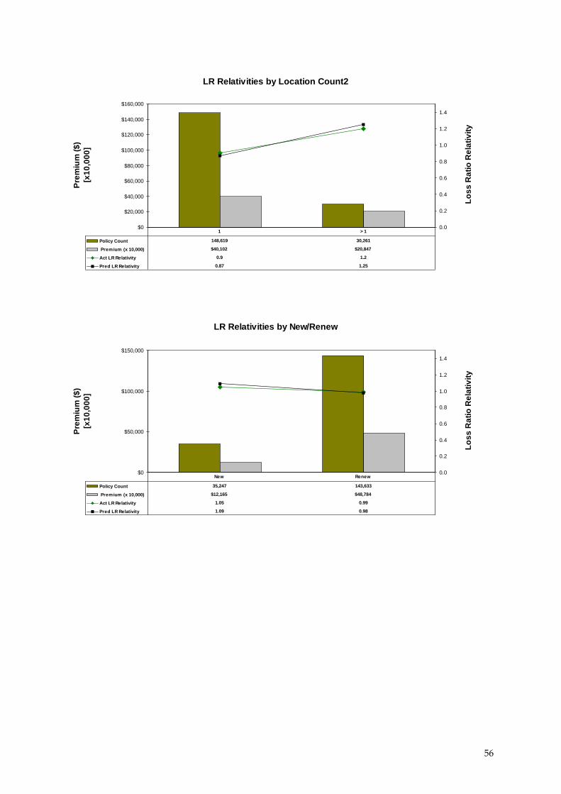
56

LR Relativities by Location Count2

$0

$20,000

$40,000

$60,000

$80,000

$100,000

$120,000

$140,000

$160,000

Pre

miu

m (

$)

[x1

0,0

00

]

0.0

0.2

0.4

0.6

0.8

1.0

1.2

1.4

Lo

ss

Ra

tio

Re

lati

vit

y


Premium (x 10,000) $40,102 $20,847



1 > 1

LR Relativities by New/Renew

$0

$50,000

$100,000

$150,000

Pre

miu

m (

$)

[x1

0,0

00

]

0.0

0.2

0.4

0.6

0.8

1.0

1.2

1.4

Lo

ss

Ra

tio

Re

lati

vit

y


Premium (x 10,000) $12,165 $48,784



New Renew

57

LR Relativities by Program Name

$0

$50,000

$100,000

$150,000

Pre

miu

m (

$)

[x1

0,0

00

]

0.0

0.2

0.4

0.6

0.8

1.0

1.2

1.4

Lo

ss

Ra

tio

Re

lati

vit

y

Policy Count 3,038 13,288 12,628 3,793 24,670 61,849 32,366 14,706 12,542

Premium (x 10,000) $2,765 $4,639 $6,059 $1,497 $7,675 $14,115 $14,475 $3,645 $6,079

Act LR Relativity 0.51 0.75 0.93 0.83 1.03 1.04 1.05 1.35 1.07

Pred LR Relativity 0.54 0.75 0.92 0.94 1 1.04 1.08 1.12 1.13

Apartment &

Condominiu

m

ContractorManufacture

rGarage Service Office Retail Professional Wholesale

LR Relativities by Limit Indicator

$0

$50,000

$100,000

$150,000

Pre

miu

m (

$)

[x1

0,0

00

]

0.0

0.2

0.4

0.6

0.8

1.0

1.2

1.4

Lo

ss

Ra

tio

Re

lati

vit

y

Policy Count 22,084 53,111 103,685

Premium (x 10,000) $12,202 $25,758 $22,989

Act LR Relativity 0.86 1.07 1

Pred LR Relativity 0.88 1.07 0.98

B BC C

58

LR Relativities by Property Deductible2

$0

$50,000

$100,000

$150,000

Pre

miu

m (

$)

[x1

0,0

00

]

0.0

0.2

0.4

0.6

0.8

1.0

1.2

1.4

Lo

ss

Ra

tio

Re

lati

vit

y

Policy Count 8,091 104,967 54,924 10,898

Premium (x 10,000) $1,408 $24,126 $25,735 $9,679



250 500 1,000 > 1,000

59

APPENDIX E: MODEL COEFFICIENTS

Commercial Auto

60

Business Owner’s Policy

61

APPENDIX F: CODE

Commercial Auto

Data Preparation

LLdataread.csv(“data.csv”,header=TRUE,sep=”,”)

LLdatasubset(LLdata,is.na(LLdata$Rerated_Prem)==FALSE)

LLdatasubset(LLdata,is.na(LLdata$CPOINTS_MODEL)==FALSE)

LLdatasubset(LLdata,LLdata$ManualPolicy==”Y”)

LLdatasubset(LLdata,(LLdata$MarketSegment==”Other”)==FALSE)

LLdatasubset(LLdata,(LLdata$LiabGrp==3)==FALSE)

LLdata$Rerated_Premifelse(LLdata$Rerated_Prem<500,500,LLdata$Rerated_Prem)

LLdata$Incurred_Lossifelse(LLdata$Incurred_Loss<0,0,LLdata$Incurred_Loss)

LLdata$Loss_RatioLLdata$Incurred_Loss/LLdata$Rerated_Prem

Capquantile(LLdata$Loss_Ratio,0.99)

LLdata$Loss_Ratioifelse(LLdata$Loss_Ratio>Cap,Cap,LLdata$Loss_Ratio)

PolEffAge2012-PoEffYear

CorpIndifelse(LLdata$Business_Type==A,1,0)

Fitting

modeltweedie.profile(Loss_Ratio~Financial_Stability+CorpInd+PolicyType+MarketSegment+PolEff

Age+FleetSize+I(FleetSize^2)+I(log(FleetSize+1))+FleetSize:PolicyType,data=LLdata,verbose=2)

fitglm(Loss_Ratio~Financial_Stability+CorpInd+PolicyType+MarketSegment+PolEffAge+

FleetSize+I(FleetSize^2)+I(log(FleetSize + 1))+FleetSize:PolicyType, family = tweedie(link.power = 0,

var.power = 1.636735), data = LLdata)

62

Lift Charts

Categorical Variables

sumPrem<-tapply(Rerated_Prem,MarketSegment,sum)

countPrem<-tapply(Rerated_Prem,MarketSegment,length)

sumLoss<-tapply(Loss_Ratio*Rerated_Prem,MarketSegment,sum)

sumPLoss<-tapply(fit22$fitted.values*Rerated_Prem,MarketSegment,sum)

LR<-sumLoss/sumPrem

PLR<-sumPLoss/sumPrem

cutoff<-data.frame(countPrem,sumPrem,sumLoss,sumPLoss,LR,PLR)

write.csv(cutoff," MarketSegment.csv")

Continuous Variables

VAR<-Financial_Stability

q <- wtd.quantile(VAR, weights=as.numeric(Rerated_Prem), probs=seq(0,1,.1), normwt=TRUE,

na.rm =TRUE)

a <- c(0,q[2],q[3],q[4],q[5],q[6],q[7],q[8],q[9],q[10],400)

quant<-rep(c("Z"),length(VAR))

for ( i in 2: (length(a))) { quant <- ifelse (Financial_Stability < a[i], ifelse (Financial_Stability >= a[i-

1], LETTERS[i-1],quant), quant)}

quant<-as.factor(quant)

sumPrem<-tapply(Rerated_Prem,quant,sum)

countPrem<-tapply(Rerated_Prem,quant,length)

sumLoss<-tapply(Loss_Ratio*Rerated_Prem,quant,sum)

sumPLoss<-tapply(fit22$fitted.values*Rerated_Prem,quant,sum)

LR<-sumLoss/sumPrem

PLR<-sumPLoss/sumPrem

lower_cut <- c(q[1],q[2],q[3],q[4],q[5],q[6],q[7],q[8],q[9],q[10])

upper_cut <- c(q[2],q[3],q[4],q[5],q[6],q[7],q[8],q[9],q[10],q[11])

63

cutoff <- data.frame(lower_cut, upper_cut, countPrem, sumPrem, sumLoss, sumPLoss, LR, PLR)

write.csv(cutoff, "Financial_Stability.csv")

Business Owners Policy

> model tweedie.profile(Loss_Ratio~Financial_Stability+EffAge+Region+Program_Name

+Control_Age+Protection_Group+Construction_Type+Property_Limit+LimitInd

+Legal_Status+Location_Count2+Property_Deductible2+NewRenew +Property_Limit:LimitInd

+Program_Name:LimitInd +NewTransfer,data=LLdata,verbose=2)

Output:

ML Estimates: xi = 1.636735 with phi= 23.55729 giving L= -49755.23

> fit29glm(Loss_Ratio~Financial_Stability+EffAge+Region+Program_Name

+Control_Age+Protection_Group+Construction_Type+Property_Limit+LimitInd

+Legal_Status+Location_Count2+Property_Deductible2+NewRenew+Property_Limit:LimitInd

+Program_Name:LimitInd +NewTransfer,data=LLdata

,family=tweedie(link.power=0,var.power=1.636735))

64

REFERENCES

Allen, R. D., Perry, M. C., Reynolds, K. V., & Long, B. P. (2008, April). Supreme Court Ruling

on the Fair Credit Reporting Act and Auto Insurers' Use of Insurance Scores to Set

Premiums. Defense Counsel Journal, 75(2), 151-160.

Anderson, M. H. (2007, June 4). Safeco, Geico Ruling Limits Credit Score Lawsuits. Market

Watch.

Factor Analysis Using SAS proc factor. (n.d.). Retrieved December 14, 2011, from UCLA:

Academic Technology Services, Statistical Consulting Group:

http://www.ats.ucla.edu/stat/sas/library/factor_ut.htm

Federal Trade Commission. (2007). Credit Based Insurance Scores: Impacts on Consumers of

Automobile Insurance.

Hanover Insurance Group. (2011, October). Personal Commmunication with Commercial

Auto Team .

Hartwig, R. P., & Wilkinson, C. (2003). The use of credit information in personal lines insurance

underwriting. New York: Insurance Information Institute.

Johnston, G. (2000). SAS Software to Fit the Generalized Linear Model. Cary, NC: SAS Institute

Inc.

Krickus, J. (2011, September 28). Experian Insurance Services. CAS Webinar.

Lipka, M. (2011, September 6). Should Using Credit Scores to Set Auto Insurance Rates be

Banned? The Boston Globe.

Massachusetts Government. (n.d.). Chapter 93: Regulation of trade and certain enterprises

(Section 62). In Administration of the government: General Laws; Regulation of Trade.

Mosley, R. (2005). The Use of Predictive Modeling in the insurance Industry. PINNACLE.

Oscherwitz, T., & Reemts, P. (2011). Alternative Credit Scores. Mortgage Banking, 71(9), 102-

105, 138.

Shi, S. (2007). Direct Analysis of Pre-Adjusted Loss Cost, Frequency or Severity in Tweedie Models.

Retrieved September 15, 2011, from Casualty Actuarial Society:

www.casact.org/pubs/forum/10wforum/shi.pdf

Suhr, D. D. ( March 26-29, 2006.). Exploratory or Confirmatory Factor Analysis? SUGI 31

Proceedings. Statistics and Data Analysis.

Suhr, D. D. (March 26-29, 2006.). Principal Component Analysis vs. Exploratory Factor

Analysis. SUGI 31 Proceedings. Statistics and Data Analysis.

Walling III, R. J. (2011, September 28). Credit-Based Tools in Commercial Lines. Pinnacle.

65

Weisbaum, H. (2010, January 27). Insurance Firms Blasted for Credit Score Rules. MSNBC.

Werner, G., & Guven, S. (2007). GLM Basic Modeling: Avoiding Common Pitfalls. Casualty

Actuarial Society Forum.

Wu, C.-S., & Guszcz, J. (2003). Does Credit Score Really Explain Insurance Losses?

Multivariate Analysis from a Data Mining Point of View. Casualty Actuarial Society

Forum, 113-138.

Documents

PREDICTIVE LOSS RATIO MODELING WITH … loss ratio modeling with credit scores, ... build sample ... 61 commercial auto