2012 RPM - Loss Cost Modeling vs FS Modeling

Loss Cost Modeling vs.

Frequency and Severity Modeling

Jun Yan Deloitte Consulting LLP

2010 CAS Ratemaking and Product Management Seminar March 21, 2011

New Orleans, LA

Antitrust Notice • The Casualty Actuarial Society is committed to adhering strictly to

the letter and spirit of the antitrust laws. Seminars conducted under the auspices of the CAS are designed solely to provide a forum for the expression of various points of view on topics described in the programs or agendas for such meetings.

• Under no circumstances shall CAS seminars be used as a means for competing companies or firms to reach any understanding – expressed or implied – that restricts competition or in any way impairs the ability of members to exercise independent business judgment regarding matters affecting competition.

• It is the responsibility of all seminar participants to be aware of antitrust regulations, to prevent any written or verbal discussions that appear to violate these laws, and to adhere in every respect to the CAS antitrust compliance policy.

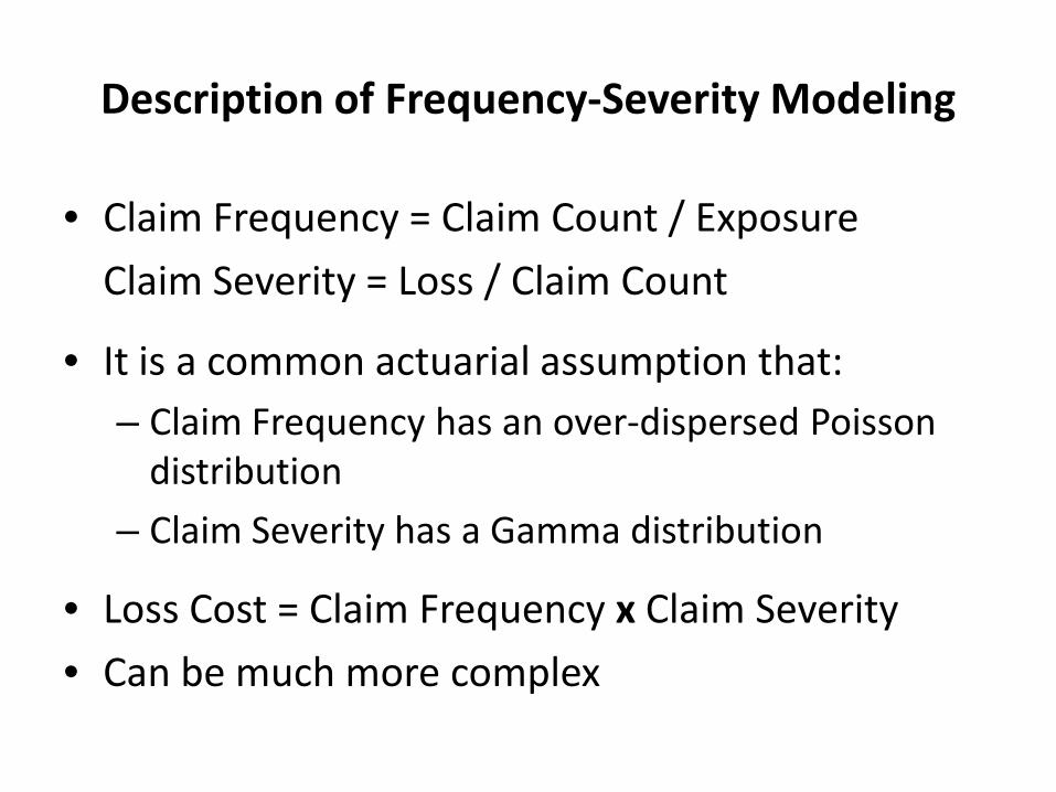
Description of Frequency-Severity Modeling

• Claim Frequency = Claim Count / Exposure Claim Severity = Loss / Claim Count

• It is a common actuarial assumption that: – Claim Frequency has an over-dispersed Poisson

distribution – Claim Severity has a Gamma distribution

• Loss Cost = Claim Frequency x Claim Severity • Can be much more complex

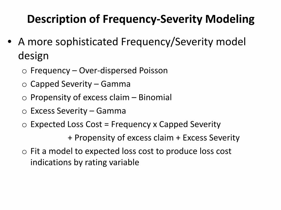
Description of Frequency-Severity Modeling

• A more sophisticated Frequency/Severity model design o Frequency – Over-dispersed Poisson o Capped Severity – Gamma o Propensity of excess claim – Binomial o Excess Severity – Gamma o Expected Loss Cost = Frequency x Capped Severity + Propensity of excess claim + Excess Severity o Fit a model to expected loss cost to produce loss cost

indications by rating variable

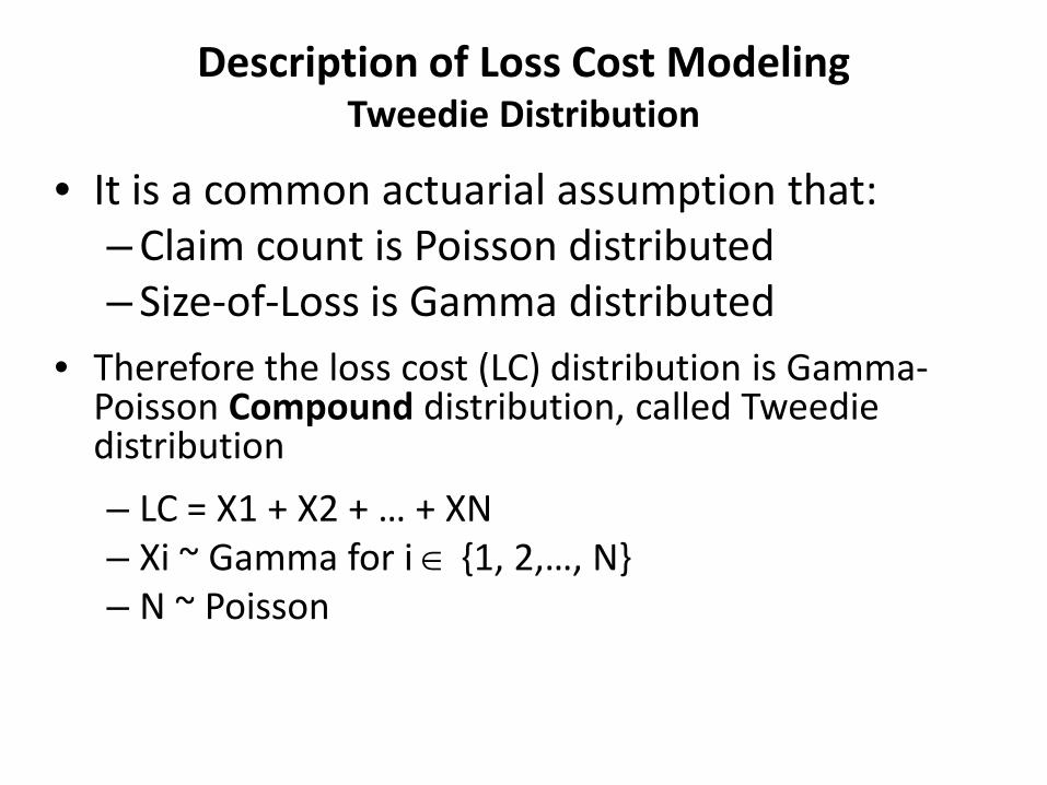
Description of Loss Cost Modeling Tweedie Distribution

• It is a common actuarial assumption that: – Claim count is Poisson distributed – Size-of-Loss is Gamma distributed

• Therefore the loss cost (LC) distribution is Gamma-Poisson Compound distribution, called Tweedie distribution

– LC = X1 + X2 + … + XN – Xi ~ Gamma for i ∈ {1, 2,…, N} – N ~ Poisson

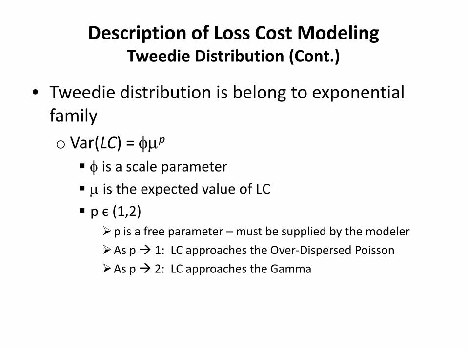
Description of Loss Cost Modeling Tweedie Distribution (Cont.)

• Tweedie distribution is belong to exponential family o Var(LC) = φµp

φ is a scale parameter µ is the expected value of LC p є (1,2)

p is a free parameter – must be supplied by the modeler As p 1: LC approaches the Over-Dispersed Poisson As p 2: LC approaches the Gamma

Data Description

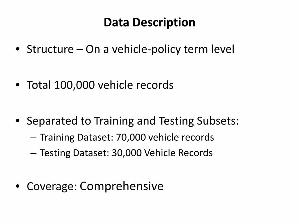
• Structure – On a vehicle-policy term level

• Total 100,000 vehicle records

• Separated to Training and Testing Subsets: – Training Dataset: 70,000 vehicle records – Testing Dataset: 30,000 Vehicle Records

• Coverage: Comprehensive

Numerical Example 1 GLM Setup – In Total Dataset

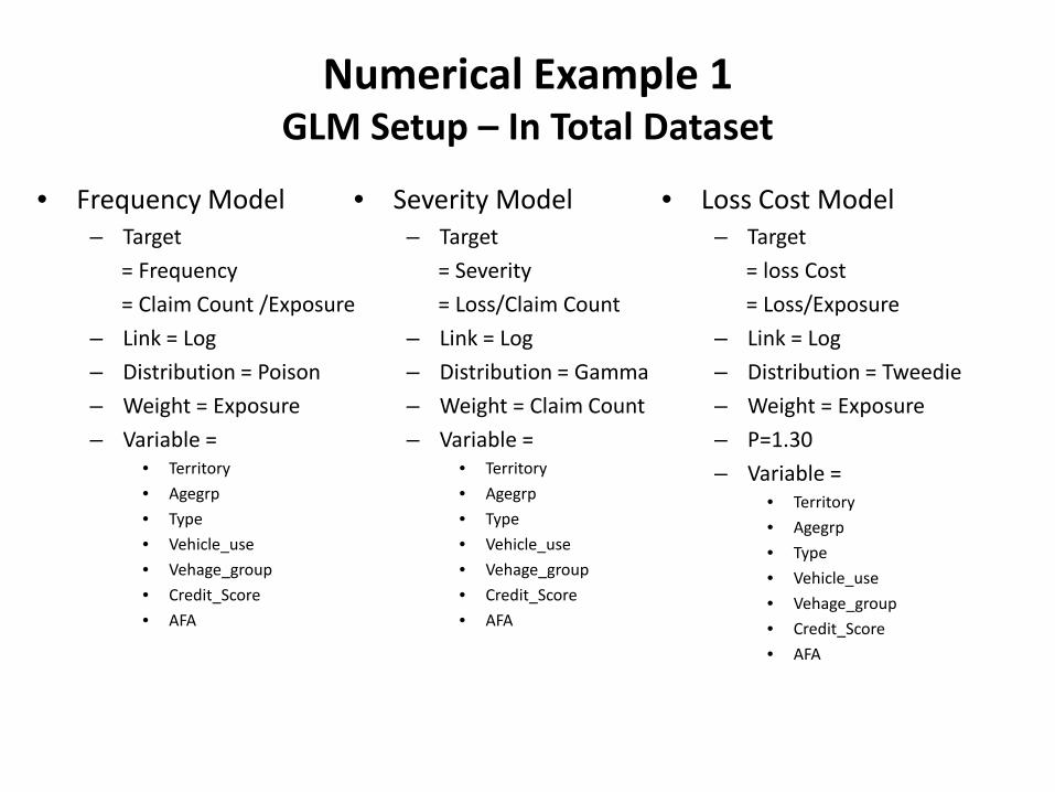
• Frequency Model – Target = Frequency = Claim Count /Exposure – Link = Log – Distribution = Poison – Weight = Exposure – Variable =

• Territory • Agegrp • Type • Vehicle_use • Vehage_group • Credit_Score • AFA

• Severity Model – Target = Severity = Loss/Claim Count – Link = Log – Distribution = Gamma – Weight = Claim Count – Variable =


• Loss Cost Model – Target = loss Cost = Loss/Exposure – Link = Log – Distribution = Tweedie – Weight = Exposure – P=1.30 – Variable =


Numerical Example 1 How to select “p” for the Tweedie model?

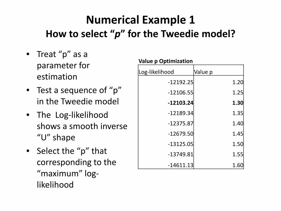
• Treat “p” as a parameter for estimation

• Test a sequence of “p” in the Tweedie model

• The Log-likelihood shows a smooth inverse “U” shape

• Select the “p” that corresponding to the “maximum” log-likelihood

Value p Optimization

Log-likelihood Value p

-12192.25 1.20

-12106.55 1.25

-12103.24 1.30

-12189.34 1.35

-12375.87 1.40

-12679.50 1.45

-13125.05 1.50

-13749.81 1.55

-14611.13 1.60

Numerical Example 1 GLM Output (Models Built in Total Data)

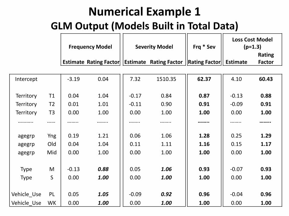
Frequency Model Severity Model Frq * Sev Loss Cost Model

(p=1.3)

Estimate Rating Factor Estimate Rating Factor Rating Factor Estimate Rating Factor

Intercept -3.19 0.04 7.32 1510.35 62.37 4.10 60.43

Territory T1 0.04 1.04 -0.17 0.84 0.87 -0.13 0.88 Territory T2 0.01 1.01 -0.11 0.90 0.91 -0.09 0.91 Territory T3 0.00 1.00 0.00 1.00 1.00 0.00 1.00 ……….. …… …….. …….. …….. …….. …….. …….. ……..

agegrp Yng 0.19 1.21 0.06 1.06 1.28 0.25 1.29 agegrp Old 0.04 1.04 0.11 1.11 1.16 0.15 1.17 agegrp Mid 0.00 1.00 0.00 1.00 1.00 0.00 1.00

Type M -0.13 0.88 0.05 1.06 0.93 -0.07 0.93 Type S 0.00 1.00 0.00 1.00 1.00 0.00 1.00

Vehicle_Use PL 0.05 1.05 -0.09 0.92 0.96 -0.04 0.96 Vehicle_Use WK 0.00 1.00 0.00 1.00 1.00 0.00 1.00

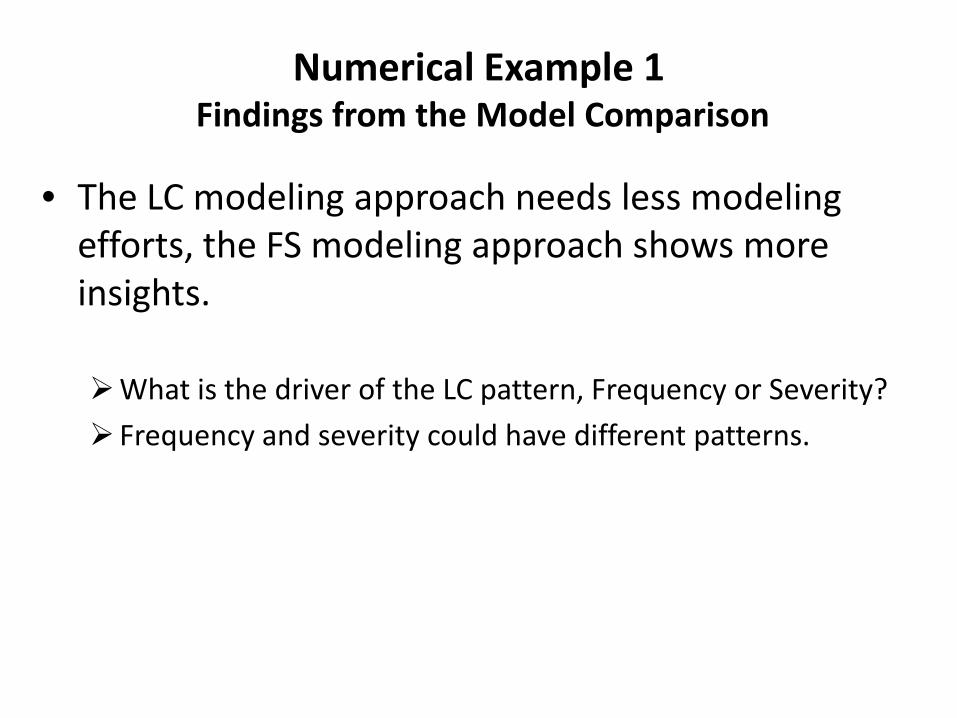
Numerical Example 1 Findings from the Model Comparison

• The LC modeling approach needs less modeling efforts, the FS modeling approach shows more insights.

What is the driver of the LC pattern, Frequency or Severity? Frequency and severity could have different patterns.

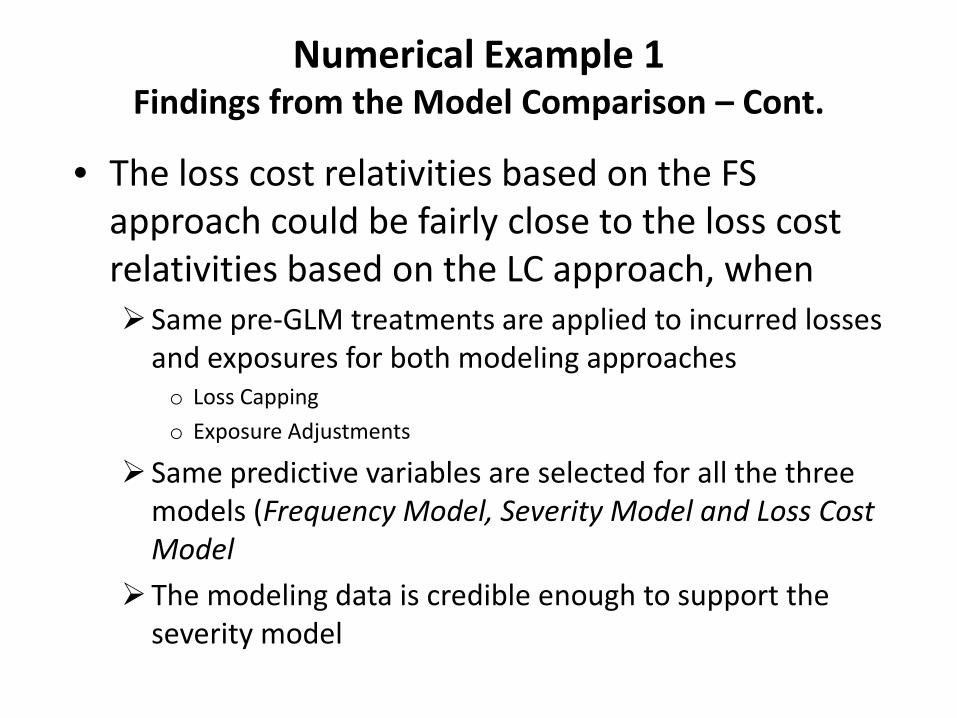
Numerical Example 1 Findings from the Model Comparison – Cont.

• The loss cost relativities based on the FS approach could be fairly close to the loss cost relativities based on the LC approach, when Same pre-GLM treatments are applied to incurred losses

and exposures for both modeling approaches o Loss Capping o Exposure Adjustments

Same predictive variables are selected for all the three models (Frequency Model, Severity Model and Loss Cost Model

The modeling data is credible enough to support the severity model

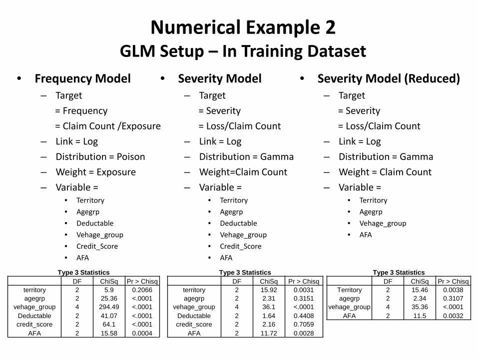
Numerical Example 2 GLM Setup – In Training Dataset

• Frequency Model – Target = Frequency = Claim Count /Exposure – Link = Log – Distribution = Poison – Weight = Exposure – Variable =

• Territory • Agegrp • Deductable • Vehage_group • Credit_Score • AFA

• Severity Model – Target = Severity = Loss/Claim Count – Link = Log – Distribution = Gamma – Weight=Claim Count – Variable =

• Territory • Agegrp • Deductable • Vehage_group • Credit_Score • AFA

• Severity Model (Reduced) – Target = Severity = Loss/Claim Count – Link = Log – Distribution = Gamma – Weight = Claim Count – Variable =

• Territory • Agegrp • Vehage_group • AFA

Type 3 Statistics DF ChiSq Pr > Chisq

territory 2 5.9 0.2066 agegrp 2 25.36 <.0001

vehage_group 4 294.49 <.0001 Deductable 2 41.07 <.0001 credit_score 2 64.1 <.0001

AFA 2 15.58 0.0004


territory 2 15.92 0.0031 agegrp 2 2.31 0.3151

vehage_group 4 36.1 <.0001 Deductable 2 1.64 0.4408 credit_score 2 2.16 0.7059

AFA 2 11.72 0.0028


Territory 2 15.46 0.0038 agegrp 2 2.34 0.3107

vehage_group 4 35.36 <.0001 AFA 2 11.5 0.0032

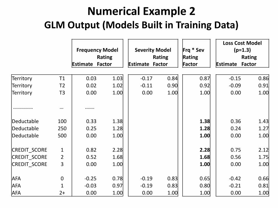
Numerical Example 2 GLM Output (Models Built in Training Data)

Frequency Model Severity Model Frq * Sev Loss Cost Model

(p=1.3)

Estimate Rating Factor Estimate

Rating Factor

Rating Factor Estimate

Rating Factor

Territory T1 0.03 1.03 -0.17 0.84 0.87 -0.15 0.86 Territory T2 0.02 1.02 -0.11 0.90 0.92 -0.09 0.91 Territory T3 0.00 1.00 0.00 1.00 1.00 0.00 1.00 …………… … ……. Deductable 100 0.33 1.38 1.38 0.36 1.43 Deductable 250 0.25 1.28 1.28 0.24 1.27 Deductable 500 0.00 1.00 1.00 0.00 1.00 CREDIT_SCORE 1 0.82 2.28 2.28 0.75 2.12 CREDIT_SCORE 2 0.52 1.68 1.68 0.56 1.75 CREDIT_SCORE 3 0.00 1.00 1.00 0.00 1.00 AFA 0 -0.25 0.78 -0.19 0.83 0.65 -0.42 0.66 AFA 1 -0.03 0.97 -0.19 0.83 0.80 -0.21 0.81 AFA 2+ 0.00 1.00 0.00 1.00 1.00 0.00 1.00

Numerical Example 2 Model Comparison In Testing Dataset

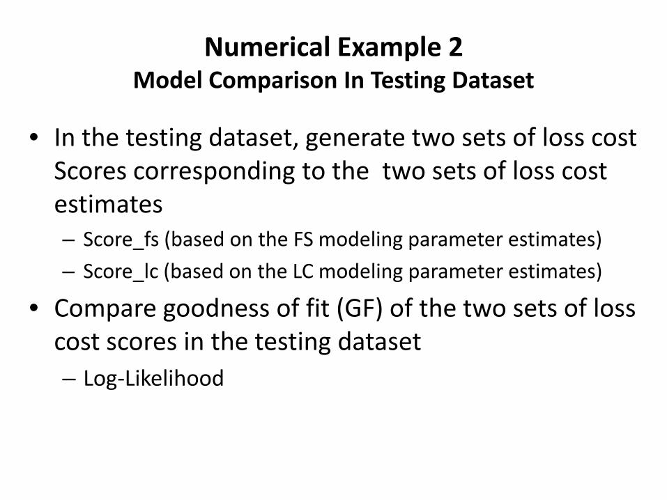
• In the testing dataset, generate two sets of loss cost Scores corresponding to the two sets of loss cost estimates – Score_fs (based on the FS modeling parameter estimates) – Score_lc (based on the LC modeling parameter estimates)

• Compare goodness of fit (GF) of the two sets of loss cost scores in the testing dataset – Log-Likelihood

Numerical Example 2 Model Comparison In Testing Dataset - Cont

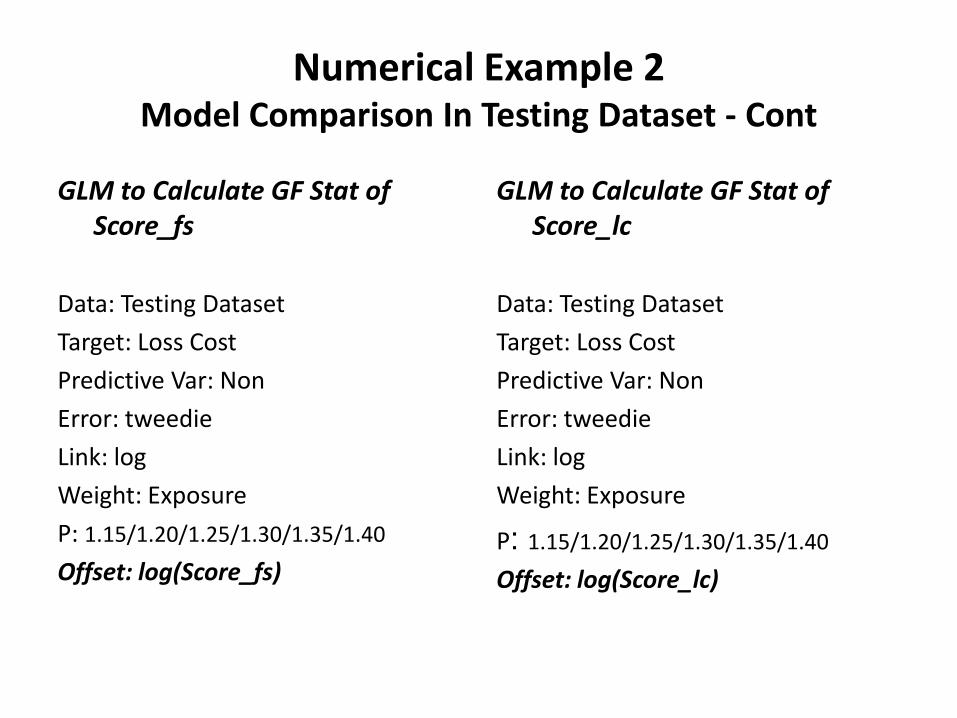
GLM to Calculate GF Stat of Score_fs

Data: Testing Dataset Target: Loss Cost Predictive Var: Non Error: tweedie Link: log Weight: Exposure P: 1.15/1.20/1.25/1.30/1.35/1.40

Offset: log(Score_fs)

GLM to Calculate GF Stat of Score_lc

Data: Testing Dataset Target: Loss Cost Predictive Var: Non Error: tweedie Link: log Weight: Exposure

P: 1.15/1.20/1.25/1.30/1.35/1.40

Offset: log(Score_lc)

Numerical Example 2 Model Comparison In Testing Dataset - Cont

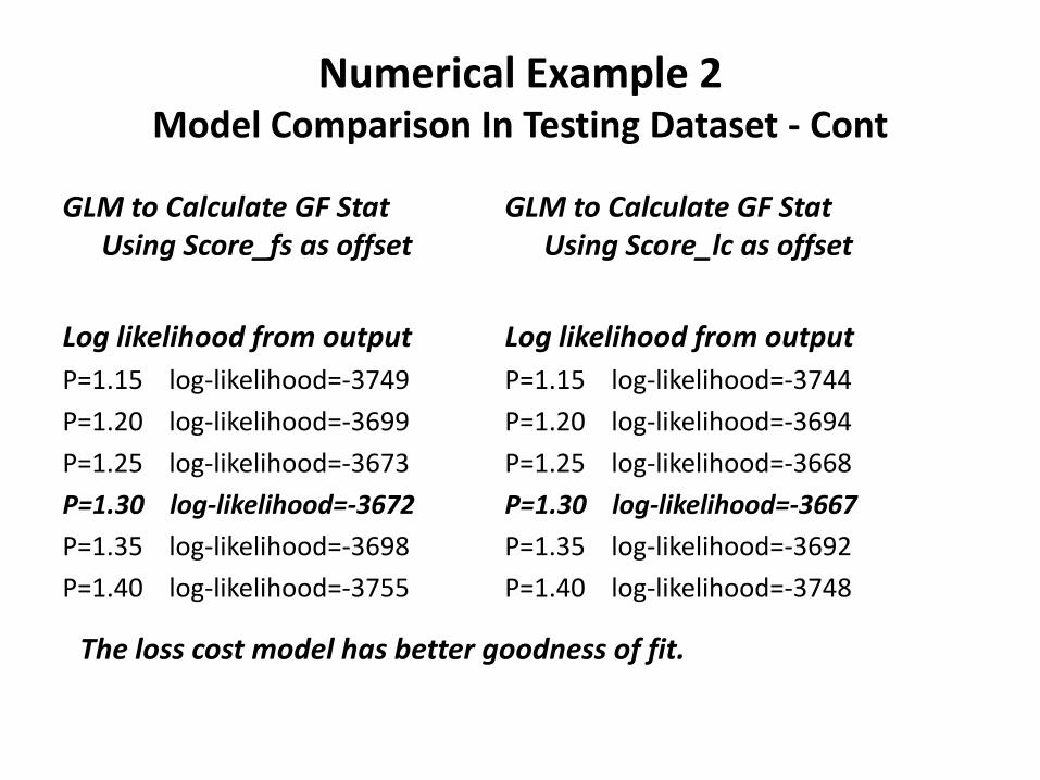
GLM to Calculate GF Stat Using Score_fs as offset

Log likelihood from output P=1.15 log-likelihood=-3749 P=1.20 log-likelihood=-3699 P=1.25 log-likelihood=-3673 P=1.30 log-likelihood=-3672 P=1.35 log-likelihood=-3698 P=1.40 log-likelihood=-3755

GLM to Calculate GF Stat Using Score_lc as offset

Log likelihood from output P=1.15 log-likelihood=-3744 P=1.20 log-likelihood=-3694 P=1.25 log-likelihood=-3668 P=1.30 log-likelihood=-3667 P=1.35 log-likelihood=-3692 P=1.40 log-likelihood=-3748

The loss cost model has better goodness of fit.

Numerical Example 2 Findings from the Model Comparison

• In many cases, the frequency model and the severity model will end up with different sets of variables. More than likely, less variables will be selected for the severity model Data credibility for middle size or small size companies For certain low frequency coverage, such as BI…

• As a result F_S approach shows more insights, but needs additional

effort to roll up the frequency estimates and severity estimates to LC relativities

In these cases, frequently, the LC model shows better goodness of fit

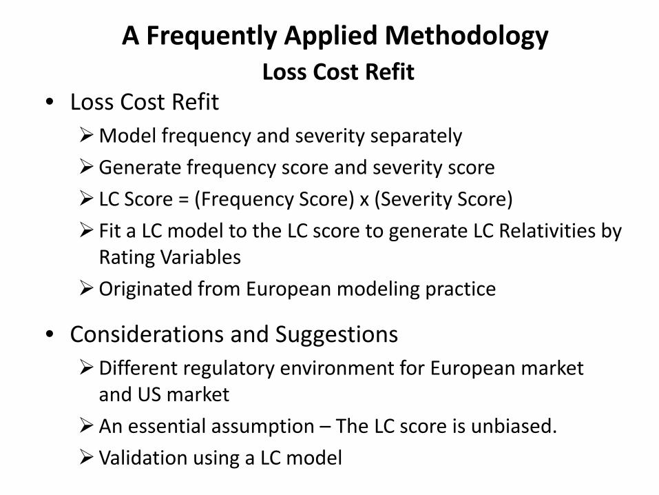
A Frequently Applied Methodology Loss Cost Refit

• Loss Cost Refit Model frequency and severity separately Generate frequency score and severity score LC Score = (Frequency Score) x (Severity Score) Fit a LC model to the LC score to generate LC Relativities by

Rating Variables Originated from European modeling practice

• Considerations and Suggestions Different regulatory environment for European market

and US market An essential assumption – The LC score is unbiased. Validation using a LC model

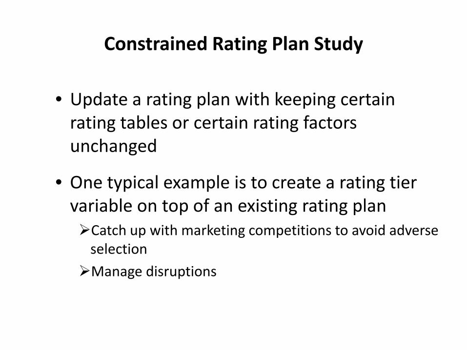
Constrained Rating Plan Study • Update a rating plan with keeping certain

rating tables or certain rating factors unchanged

• One typical example is to create a rating tier variable on top of an existing rating plan Catch up with marketing competitions to avoid adverse

selection Manage disruptions

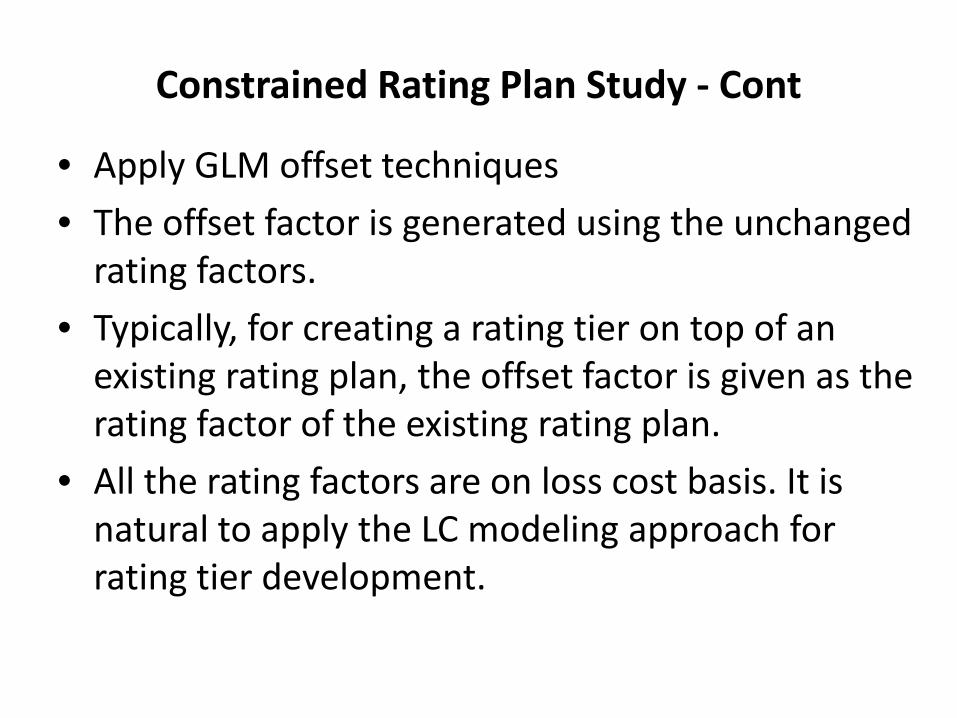
Constrained Rating Plan Study - Cont

• Apply GLM offset techniques • The offset factor is generated using the unchanged

rating factors. • Typically, for creating a rating tier on top of an

existing rating plan, the offset factor is given as the rating factor of the existing rating plan.

• All the rating factors are on loss cost basis. It is natural to apply the LC modeling approach for rating tier development.

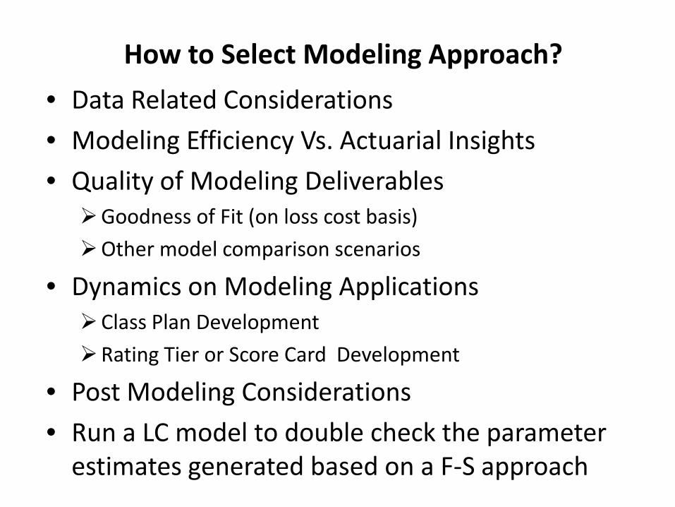
How to Select Modeling Approach? • Data Related Considerations • Modeling Efficiency Vs. Actuarial Insights • Quality of Modeling Deliverables Goodness of Fit (on loss cost basis) Other model comparison scenarios

• Dynamics on Modeling Applications Class Plan Development Rating Tier or Score Card Development

• Post Modeling Considerations • Run a LC model to double check the parameter

estimates generated based on a F-S approach

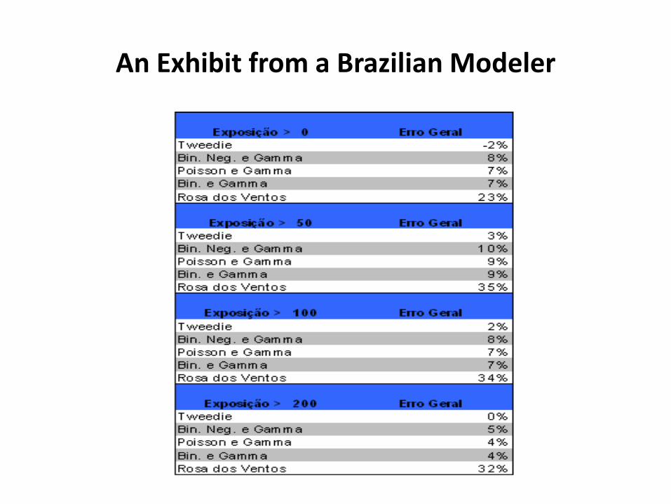
An Exhibit from a Brazilian Modeler

Documents

2012 RPM - Loss Cost Modeling vs FS Modeling