PREDICTION OF PIPE PERFORMANCE WITH MACHINE LEARNING USING R

Name: XXXXXX

Student Number: XXXXXXX

2016-11-29

1. Instruction

As one of the most important infrastructures in cities, water mains buried underground require

an efficient infrastructure management system to manage complicated deteriorating pipeline

systems, since the failure of pipeline can result in high maintenance cost and serious threats to

society and the environment. The core component of the management system is the technology for

condition assessment of water mains, specifically, methods to evaluate the pipeline condition and

methods to predict the pipe’s remaining service life. Hence, lots of studies have been undertaken,

utilizing data to develop a decision model to assess the pipe performance and analyze the key

factors leading to pipeline failure.

For water mains assessment, statistical models are a cost-effective means of analysis. The

generalized multivariate exponential model proposed by Kleiner and Rajani et al. (2003)

considered time-dependent variables and allows for simple evaluation and variation prediction in

pipe breaks. Multivariate exponential model was also developed, compared with transition state-

life regression model and validated later (Osman, Ph, & Bainbridge, 2011). Recently, another

statistical model: a Bayesian belief network model (BNN) was proposed, which used soil

properties to predict the remaining service life of water mains (Demissie, Tesfamariam, & Sadiq,

2014). It determined soil corrosion index by sorting the soil parameters into major groups and

minor groups. Then, combining with a mathematical model, the safety index is calculated with pit

depth, corrosion initiation time and pipe wall thickness using BBN. Such statistical approaches

mentioned above may help pipeline management by predicting remaining service life or break rate

of water mains. However, in parallel with the statistical approaches, the complexity of water

networks has led to wider employment of data mining techniques to predict pipe failures (Berardi,

Giustolisi, Kapelan, & Savic, 2008).

Based on data mining techniques, artificial neural networks (ANN) methods have been widely

employed in pipe’s performance prediction. To improve previous failure prediction of pipelines,

ANN model: multilayer perceptron (MLP) is proposed (Achim, Ghotb, & Mcmanus, 2007). It

achieved an improvement 19% in terms of 𝑟2 when compared with shifted time exponential model.

Then a model integrated Analytical Hierarchy Process and ANN was developed (Al-barqawi &

Zayed, 2008). After utilizing AHP to determine weights of factors and their sub-factors, supervised

ANN and back propagation algorithm were used to predict pipe performance and its deterioration

rate. Fahmy et al. (2009) applied multiple regression, MLP and general regression neural network

(GRNN) to forecast the remaining useful life of cast iron water mains. Considering two

rehabilitation strategies: Cement Mortar Lining and Cathodic Protection, Asnaashari et al. (2013)

predicted the watermain failure rates successfully using ANN modelling.

However, in a recent study, when GRNN and Feed Forward Neural Networks were used to

estimate the pipe failure rates, their performance was worse than that of a novel approach

combining fuzzy clustering and least square support vector machine (LS-SVM) (Aydogdu & Firat,

2015). Through the review of previous studies, integrated modelling tends to have a more

outstanding prediction performance because they would have the advantages of two or more

models. Therefore, this project presents a stacking ensemble prediction method, combining the

predictions from different advanced models, to modify existing models. Armed with the tools

learnt from the class, this project first used Excel to do data transformation, cleaning and some

basic data analysis. Then cleaned data was read into R to do more data visualization and analysis

first based on ggplot package. Finally, machine learning was employed to predict the pipe

performance based on the caret package in R.

2. Data Description

The original dataset is a xlsx file which contains 119 rows and 19 columns data with missing

values and irrelevant variables. These datasets of water mains were collected from Toronto (Doyle,

2000) including pipe identity, external pit depth, internal pit depth, pipe age, pipe wall thickness

and five soil properties.

3. Overview of Techniques

Based on the techniques covered in the class, Microsoft Excel and R were selected in this

project. Microsoft Excel is the most popular spreadsheet program that allows users to quickly sort,

analyze and report data. In this project, Excel was used to do data transformation and data cleaning.

For R, it is an open source programming language for statistical computing and graphics with the

most comprehensive available statistical analysis package. Since the graphical capabilities of R

are outstanding, it was utilized to visualize data based on the ggplot package in this project. With

respect to machine learning, the caret package in R offers a nifty way of developing it. In addition,

since the new technology and ideas often appear first in R, ensemble method implemented was

based on the latest package in R, caretEnsemble.

4. Data Cleaning Using Excel

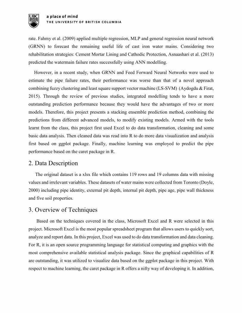
Because of the difficulty of collecting data related to soil properties and pipe features, shown

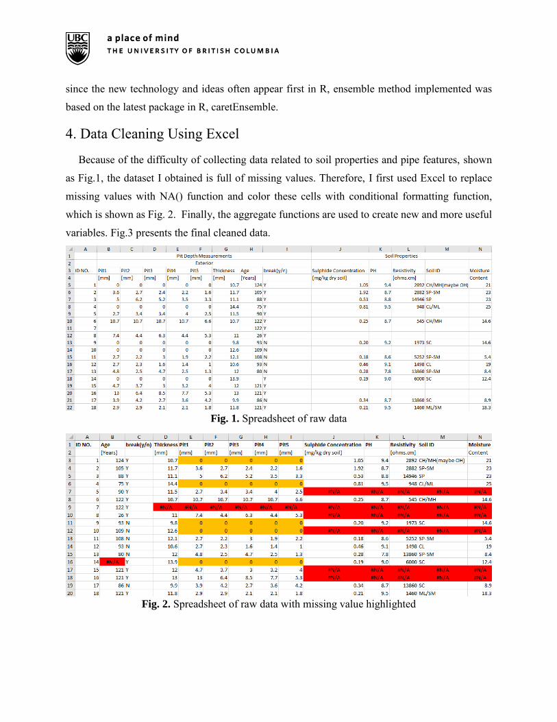
as Fig.1, the dataset I obtained is full of missing values. Therefore, I first used Excel to replace

missing values with NA() function and color these cells with conditional formatting function,

which is shown as Fig. 2. Finally, the aggregate functions are used to create new and more useful

variables. Fig.3 presents the final cleaned data.

Fig. 1. Spreadsheet of raw data

Fig. 2. Spreadsheet of raw data with missing value highlighted

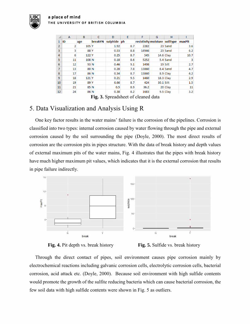
Fig. 3. Spreadsheet of cleaned data

5. Data Visualization and Analysis Using R

One key factor results in the water mains’ failure is the corrosion of the pipelines. Corrosion is

classified into two types: internal corrosion caused by water flowing through the pipe and external

corrosion caused by the soil surrounding the pipe (Doyle, 2000). The most direct results of

corrosion are the corrosion pits in pipes structure. With the data of break history and depth values

of external maximum pits of the water mains, Fig. 4 illustrates that the pipes with break history

have much higher maximum pit values, which indicates that it is the external corrosion that results

in pipe failure indirectly.

Fig. 4. Pit depth vs. break history Fig. 5. Sulfide vs. break history

Through the direct contact of pipes, soil environment causes pipe corrosion mainly by

electrochemical reactions including galvanic corrosion cells, electrolytic corrosion cells, bacterial

corrosion, acid attack etc. (Doyle, 2000). Because soil environment with high sulfide contents

would promote the growth of the sulfite reducing bacteria which can cause bacterial corrosion, the

few soil data with high sulfide contents were shown in Fig. 5 as outliers.

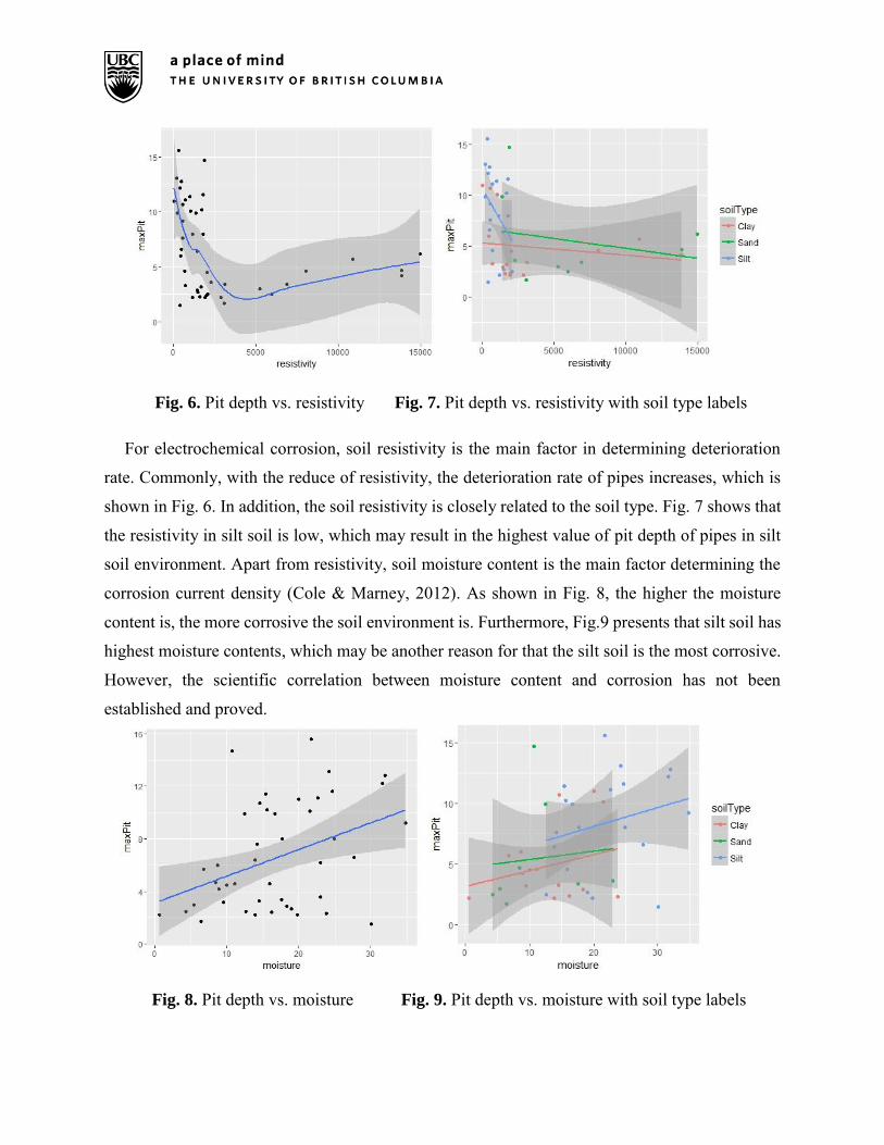
Fig. 6. Pit depth vs. resistivity Fig. 7. Pit depth vs. resistivity with soil type labels

For electrochemical corrosion, soil resistivity is the main factor in determining deterioration

rate. Commonly, with the reduce of resistivity, the deterioration rate of pipes increases, which is

shown in Fig. 6. In addition, the soil resistivity is closely related to the soil type. Fig. 7 shows that

the resistivity in silt soil is low, which may result in the highest value of pit depth of pipes in silt

soil environment. Apart from resistivity, soil moisture content is the main factor determining the

corrosion current density (Cole & Marney, 2012). As shown in Fig. 8, the higher the moisture

content is, the more corrosive the soil environment is. Furthermore, Fig.9 presents that silt soil has

highest moisture contents, which may be another reason for that the silt soil is the most corrosive.

However, the scientific correlation between moisture content and corrosion has not been

established and proved.

Fig. 8. Pit depth vs. moisture Fig. 9. Pit depth vs. moisture with soil type labels

6. Prediction of Pipe Performance Using R

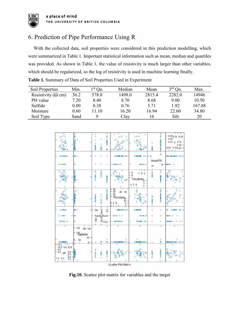
With the collected data, soil properties were considered in this prediction modelling, which

were summarized in Table 1. Important statistical information such as mean, median and quartiles

was provided. As shown in Table 1, the value of resistivity is much larger than other variables,

which should be regularized, so the log of resistivity is used in machine learning finally.

Table 1. Summary of Data of Soil Properties Used in Experiment

Soil Properties Min. 1st Qu. Median Mean 3rd Qu. Max. Resistivity (Ω cm) 36.2 578.0 1498.0 2815.4 2282.0 14946 PH value 7.20 8.40 8.70 8.68 9.00 10.50 Sulfide 0.00 0.38 0.76 5.71 1.92 167.88 Moisture 0.60 11.10 16.20 16.94 22.60 34.80 Soil Type Sand 9 Clay 16 Silt 20

Fig.10. Scatter plot matrix for variables and the target

To evaluate pipe condition, pipe deterioration rate (DR) was used as the predictive target in this

experiment, which was expressed as the ratio between the maximum pitting depth and pipe age

(Liu, Sadiq, Rajani, & Najjaran, 2010). Then, corresponding scatter plot with the DR as 𝑦 was

shown in Fig. 10, which provided an overview of the relationship between every two variables. As

depicted in Fig.10, the plot relating DR to pH are scattered randomly, which may indicate there is

no strong correlation between the soil pH and DR.

6.1 Random Forest (RF)

RF gets its name from the concept that each tree is grown with a randomized subset of predictors,

and that a forest consists of a large number of trees (Liu et al., 2010). It starts with a standard

machine learning technique, decision tree. Not only does it has fast runtimes, but it also can deal

with unbalanced and missing data. However, it also has disadvantage that when it is used for

regression, it may overfit datasets that are particularly noisy. As an ensemble method, the random

forest was first tried in this project.

6.2 Gaussian Process

A Gaussian process is a collection of random variables that have joint Gaussian distributions,

which can be employed as a supervised learning method to solve flexible non-linear regression

problems. The appearance of kernel machines such as SVM and Gaussian opens the new

perspectives with practical prediction and nonlinear modeling (Rasmussen, 2006). Therefore,

Gaussian process with a radial basis function (RBF) kernel model was built in this study to help

predict DR of pipelines. The RBF kernel is stationary kernel, which can be expressed as following:

κ(𝑥𝑖 , 𝑥𝑗) = 𝑒𝑥𝑝 (−𝑑(𝑥𝑖 𝑙⁄ ,𝑥𝑗/𝑙)

2

2) (1)

where ι > 0, which is a length-scale hyperparameter (Yang, Smola, Song, & Wilson, 2015).

6.3 SVM

The SVM algorithm derived from a nonlinear generalization of generalized portrait algorithm

in 1993 and entered the standard methods toolbox of machine learning in around 1998 (Smola &

Schölkopf, 2004). The SVM is scalable, which can generalize well, even on relatively small given

training data sets (Suykens & Vandewalle, 2000). The SVM is applied to regression problems by

the introduction of an alternative loss function (Brereton & Lloyd, 2010). In this experiment, SVM

with a RBF kernel was used to predict the pipe performance. In the training process, two

parameters should be noticed: λ and c. λ parameter defines the influence weights of a single

training examples while c parameter weights the error of training samples against simplicity of

decision surface. After model tuning, the final parameters used for the model were λ = 0.0245517

and c = 1.

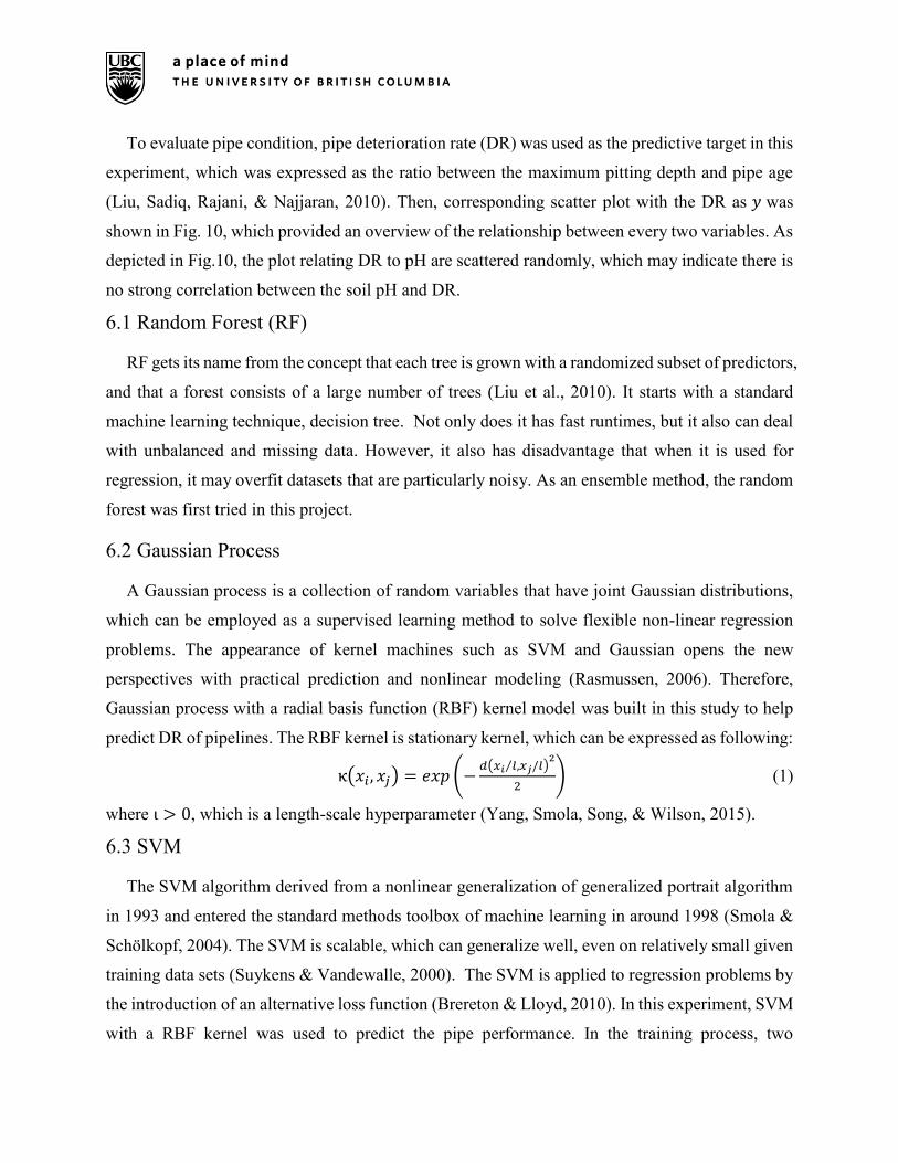
6.4 Combine Model Prediction into Ensemble Predictions

Stacking is about combining multiple models built by using different learning algorithm on the

same dataset. After a set of base-level models are built and evaluated, a meta-level model is

introduced to learn how to combine the results of the base-level models (Dzeroski & Zenko, 2004).

Intuitively, ensembles allow the different needs of a difficult problem to be handled by models

suited to those particular needs (Oza & Tumer, 2008). In this study, stacking ensemble method

used higher-order model, generalized linear model (GLM) to learn how to best combine two best

performance models: Gaussian and SVM.

Fig.11. Flowchart of methodology of stacking ensemble

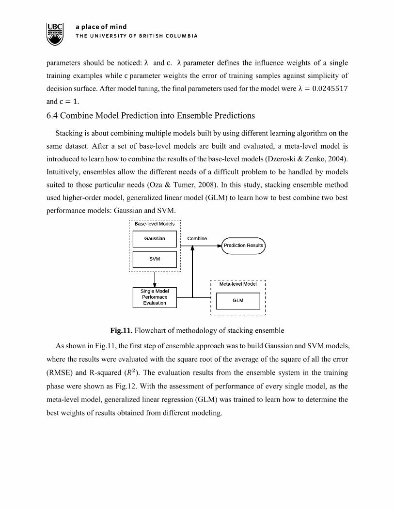
As shown in Fig.11, the first step of ensemble approach was to build Gaussian and SVM models,

where the results were evaluated with the square root of the average of the square of all the error

(RMSE) and R-squared (𝑅2). The evaluation results from the ensemble system in the training

phase were shown as Fig.12. With the assessment of performance of every single model, as the

meta-level model, generalized linear regression (GLM) was trained to learn how to determine the

best weights of results obtained from different modeling.

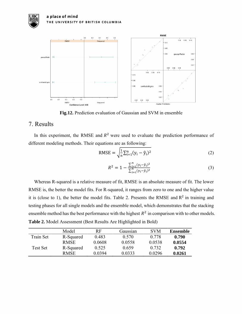
Fig.12. Prediction evaluation of Gaussian and SVM in ensemble

7. Results

In this experiment, the RMSE and 𝑅2 were used to evaluate the prediction performance of

different modeling methods. Their equations are as following:

RMSE = √1

n∑ (yi − yi)2ni=1 (2)

𝑅2 = 1 −∑ (𝑦𝑖−𝑖)

2𝑛

𝑖=1

∑ (𝑦𝑖−𝑖)2𝑛

𝑖=1

(3)

Whereas R-squared is a relative measure of fit, RMSE is an absolute measure of fit. The lower

RMSE is, the better the model fits. For R-squared, it ranges from zero to one and the higher value

it is (close to 1), the better the model fits. Table 2. Presents the RMSE and R2 in training and

testing phases for all single models and the ensemble model, which demonstrates that the stacking

ensemble method has the best performance with the highest 𝑅2 in comparison with to other models.

Table 2. Model Assessment (Best Results Are Highlighted in Bold)

Model RF Gaussian SVM Ensemble

Train Set R-Squared 0.483 0.570 0.778 0.790

RMSE 0.0608 0.0558 0.0538 0.0554

Test Set R-Squared 0.525 0.659 0.732 0.792

RMSE 0.0394 0.0333 0.0296 0.0261

Even though the data collected is small, the ensemble modeling proposed in this paper still has

a good prediction performance with the highest 𝑅2 value of 0.792 and the lowest RMSE value of

0.0261. Compared with Gaussian and SVM modeling, its accuracy of the prediction also has a

certain level of improvement.

8. Conclusion Since the need to assess watermain performance efficiently is growing, forecasting the

condition of water main becomes increasingly important. This project employed a novel approach

to better forecast the pipe performance based on machine learning with stacking ensemble

modeling. Four models including the ensemble model were implemented to predict the condition

of pipelines. Compared with the performance of RF, Gaussian and SVM models, the superiority

of ensemble methods is demonstrated, reducing the RMSE up to 45%. Since the ensemble

modeling developed in this paper is robust and accurate, it can assist pipe management system to

do pipe performance measure using data of soil properties.

Reference Achim, D., Ghotb, F., & Mcmanus, K. J. (2007). Prediction of Water Pipe Asset Life Using

Neural Networks, 13(1), 26–30.

Al-barqawi, H., & Zayed, T. (2008). Infrastructure Management: Integrated AHP / ANN Model to Evaluate Municipal Water Mains ’ Performance, 14(December), 305–318.

Aydogdu, M., & Firat, M. (2015). Estimation of Failure Rate in Water Distribution Network Using Fuzzy Clustering and LS-SVM Methods, 1575–1590. http://doi.org/10.1007/s11269-014-0895-5

Berardi, L., Giustolisi, O., Kapelan, Z., & Savic, D. a. (2008). Development of pipe deterioration models for water distribution systems using EPR. Journal of Hydroinformatics, 10(2), 113. http://doi.org/10.2166/hydro.2008.012

Brereton, R. G., & Lloyd, G. R. (2010). Support vector machines for classification and regression. The Analyst, 135(2), 230–267. http://doi.org/10.1039/b918972f

Cole, I. S., & Marney, D. (2012). The science of pipe corrosion: A review of the literature on the corrosion of ferrous metals in soils. Corrosion Science, 56, 5–16. http://doi.org/10.1016/j.corsci.2011.12.001

Demissie, G., Tesfamariam, S., & Sadiq, R. (2014). Considering soil parameters in prediction of remaining service life of metallic pipes: a Bayesian belief network model. Journal of

Pipeline Systems Engineering and PracticePipeline Systems -Engineering and Practice, 7(1994), 1–12. http://doi.org/10.1061/(ASCE)PS.1949-1204.0000229.

Doyle, G. (2000). The Role Of Soil In The External Corrosion Of Cast-Iron Water Mains In

Toronto , Canada. A Thesis for M.A.Sc.

Dzeroski, S., & Zenko, B. (2004). Is combining classifiers with stacking better than selecting the best one? Machine Learning, 54(3), 255–273. http://doi.org/10.1023/B:MACH.0000015881.36452.6e

Liu, Z., Sadiq, R., Rajani, B., & Najjaran, H. (2010). Exploring the Relationship between Soil Properties and Deterioration of Metallic Pipes Using Predictive Data Mining Methods, 24(June), 289–301.

Osman, H., Ph, D., & Bainbridge, K. (2011). Comparison of Statistical Deterioration Models for Water Distribution Networks, 25(June), 259–266. http://doi.org/10.1061/(ASCE)CF.1943-5509

Oza, N. C., & Tumer, K. (2008). Classifier ensembles: Select real-world applications. Information Fusion, 9(1), 4–20. http://doi.org/10.1016/j.inffus.2007.07.002

Rasmussen, C. E. (2006). Gaussian processes for machine learning. International Journal of

Neural Systems, 14(2), 69–106. http://doi.org/10.1142/S0129065704001899

Smola, A. J., & Schölkopf, B. (2004). A tutorial on support vector regression. Statistics and

Computing, 14(3), 199–222. http://doi.org/10.1023/B:STCO.0000035301.49549.88

Suykens, J., & Vandewalle, J. (2000). Recurrent Least Squares Support Vector Machines. Circuits and Systems I: …, 47(7), 349–354. Retrieved from http://ieeexplore.ieee.org/xpls/abs_all.jsp?arnumber=855471

Yang, Z., Smola, A. J., Song, L., & Wilson, A. G. (2015). A la Carte — Learning Fast Kernels. Aistats, 38.