Prediction of gas holdup in a column flotation cell using … · 2019-03-07 · Prediction of gas holdup in a column flotation cell using computational fluid dynamics (CFD) 2009;

Column flotation is an important concentrationtechnology that is used in the mineralprocessing and coal beneficiation industries.The growing interest in the use of columnflotation in mineral processing has beenattributed to the simpler flotation circuits andimproved metallurgical performance comparedto conventional flotation cells (Finch andDobby, 1990). Flotation columns have alsofound other applications outside mineralprocessing, such as de-inking of recycledpaper (Finch and Hardie, 1999).

In column flotation, a rising swarm of airbubbles generated by means of air spargers isemployed to collect the valuable mineralparticles and separate them from the gangueminerals in a countercurrent process. Washwater, which is continuously fed at the top ofthe column, is used to eliminate entrainedparticles and stabilize the froth. The columnvolume can be divided into two sections – thecollection zone in which the bubbles collect thefloatable mineral particles, and the cleaningzone (or froth zone) where product upgradingis enhanced through the removal of unwanted

particles entrained in the water mixed withbubbles from the collection zone.

One of the most important operationalvariables affecting the metallurgicalperformance of flotation columns is gas holdupin the collection zone (Gomez et al., 1991).Gas holdup is defined as the volumetricfraction (or percentage) occupied by gas at anypoint in a column (Finch and Dobby, 1990).Some studies have reported that gas holdupaffected both the recovery and grade inindustrial and pilot-scale flotation columns(Leichtle, 1998; López-Saucedo et al., 2012).These studies reported a linear relationshipbetween gas holdup and recovery. Linearrelationships between gas holdup and theflotation rate constant have also beenidentified, highlighting its effect on flotationkinetics (Hernandez, Gomez, and Finch, 2003;Massinaei et al., 2009). On the other hand,other researchers have suggested that gasholdup could be used for control purposes incolumn flotation (Dobby, Amelunxen, andFinch, 1985). However, apart from its potentialin control, gas holdup also has diagnosticapplications, for example the sudden drop ingas holdup that occurs when a sparger ismalfunctioning.

Because of its importance in columnflotation, gas holdup has been studied byseveral researchers who have reported averageand local gas holdup measurements in thecolumn (Gomez et al., 1991, 1995; Paleari, Xu,and Finch, 1994; Tavera, Escudero, and Finch,2001). Computational fluid dynamics (CFD)has emerged as a numerical modelling toolthat can be used to enhance the understandingof the complex hydrodynamics pertaining toflotation cells (Deng, Mehta, and Warren,1996; Koh et al., 2003; Koh and Schwarz,

Prediction of gas holdup in a columnflotation cell using computational fluiddynamics (CFD)by I. Mwandawande*, G. Akdogan*, S.M. Bradshaw*, M. Karimi†, and N. Snyders*

Computational fluid dynamics (CFD) was applied to predict the averagegas holdup and the axial gas holdup variation in a 13.5 m high cylindricalcolumn 0.91 m diameter. The column was operating in batch mode. AEulerian-Eulerian multiphase approach with appropriate interphasemomentum exchange terms was applied to simulate the gas-liquid flowinside the column. Turbulence in the continuous phase was modelled usingthe k-� realizable turbulence model. The predicted average gas holdupvalues were in good agreement with experimental data. The axial gasholdup prediction was generally good for the middle and top parts of thecolumn, but was over-predicted for the bottom part of the column. Bubblevelocity profiles were observed in which the axial velocity of the airbubbles decreased with height in the column. This may be related to theupward increase in gas holdup in the column. Simulations were alsoconducted to compare the gas holdup predicted with the universal, theSchiller-Naumann, and the Morsi-Alexander drag models. The gas holduppredictions for the three drag models were not significantly different.

column flotation, computational fluid dynamics (CFD), gas holdup.

* University of Stellenbosch, South Africa.† Chalmers University of Technology, Gothenburg,

Sweden.© The Southern African Institute of Mining and

Metallurgy, 2019. ISSN 2225-6253. Paper receivedDec. 2017; revised paper received Mar. 2018.

81VOLUME 119 �

http://dx.doi.org/10.17159/2411-9717/2019/v119n1a10

Prediction of gas holdup in a column flotation cell using computational fluid dynamics (CFD)

2009; Chakraborty, Guha, and Banerjee, 2009). For columnflotation cells, CFD modelling has been applied to predict theaverage gas holdup for the whole column (Koh and Schwarz,2009; Chakraborty, Guha, and Banerjee, 2009). However, thegas holdup has been observed to vary with height along thecollection zone of the flotation column (Gomez et al., 1991,1995; Yianatos et al., 1995), increasing by almost 100% fromthe bottom to the top of the column. The increase in gasholdup with height is attributed to the hydrostatic expansionof bubbles (Yianatos et al., 1995; Zhou and Egiebor, 1993).

Despite the reported increase in gas holdup along thecolumn height, the CFD literature on column flotation doesnot account for this phenomenon. This could result in theunder-prediction of gas holdup, particularly in cases wherethe available experimental measurements were taken nearthe top of the column. For example, Koh and Schwarz (2009)reported an average gas holdup of 0.176 for the wholecolumn compared with 0.23 measured at the top part of thecolumn. The height of this column was 4.9 m. Industrialflotation columns are typically 9-15 m high (Finch andDobby, 1990). This highlights the significance of consideringthe axial gas holdup variation in column flotation CFDmodels.

The aim of the present work was therefore to investigatethe application of CFD for predicting not only the average gasholdup, but also the axial gas holdup variation in the column.In this regard, CFD was used to model a cylindrical pilotcolumn that was used in previous studies on axial gas holdupdistribution (Gomez et al., 1991, 1995). Since thecorresponding experimental work was performed in two-phase systems with water and air only (in the presence of afrother), two-phase simulations were conducted in thepresent study in order to simulate the actual conditions in thepilot column.

In an attempt to understand the observed axial variationsin gas holdup, Sam. Gomez, and Finch (1996) conductedexperiments in which axial velocity profiles of single bubbleswere measured. However, column flotation involves a swarmof bubbles as opposed to single bubbles. Swarms of movingbubbles are known to have velocities that are different fromthose derived for the case of single bubbles (Gal-Or andWaslo, 1968; Delnoij, Kuipers, and van Swaaij, 1997). CFD iscapable of predicting the entire flow fields of the variousphases involved in the flotation process. For this reason, CFDis a suitable tool that can be used to simulate the axialvariation in bubble velocity in order to understand the spatialgas holdup distribution in the column. Axial bubble velocityprofiles are therefore included in this study in the context oftheir possible relationship with the axial gas holdup profilealong the column height.

The pilot flotation column was used in previous research(Gomez et al., 1991, 1995) to study gas holdup in thecollection zone. It has a diameter of 0.91 m and a height ofapproximately 13.5 m. The experimental work was conductedwith air and water only in a batch process. Air wasintroduced into the column through three Cominco-typespargers.

This column was selected for the present CFD modellingstudies because axial gas holdup variation had been earlier

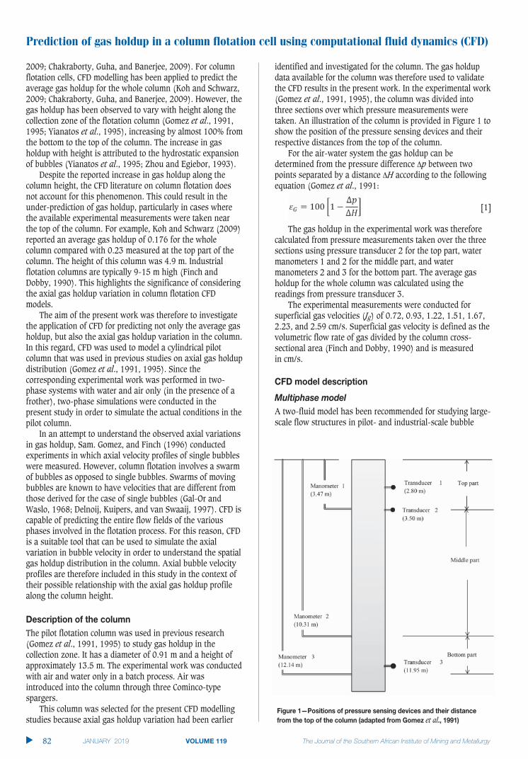
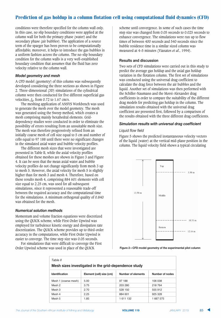
identified and investigated for the column. The gas holdupdata available for the column was therefore used to validatethe CFD results in the present work. In the experimental work(Gomez et al., 1991, 1995), the column was divided intothree sections over which pressure measurements weretaken. An illustration of the column is provided in Figure 1 toshow the position of the pressure sensing devices and theirrespective distances from the top of the column.

For the air-water system the gas holdup can bedetermined from the pressure difference p between twopoints separated by a distance H according to the followingequation (Gomez et al., 1991:

[1]

The gas holdup in the experimental work was thereforecalculated from pressure measurements taken over the threesections using pressure transducer 2 for the top part, watermanometers 1 and 2 for the middle part, and watermanometers 2 and 3 for the bottom part. The average gasholdup for the whole column was calculated using thereadings from pressure transducer 3.

The experimental measurements were conducted forsuperficial gas velocities (Jg) of 0.72, 0.93, 1.22, 1.51, 1.67,2.23, and 2.59 cm/s. Superficial gas velocity is defined as thevolumetric flow rate of gas divided by the column cross-sectional area (Finch and Dobby, 1990) and is measured in cm/s.

A two-fluid model has been recommended for studying large-scale flow structures in pilot- and industrial-scale bubble

�

82

et al

columns, due to its relatively low computational cost (Delnoij,Kuipers, and van Swaaij, 1997). A Eulerian-Eulerian two-fluid model was therefore selected in the present research,considering the large size of the pilot flotation column thatwas to be modelled. Subsequent CFD simulations in thisstudy were performed using the Ansys Fluent 14.5 softwarepackage.

In the Eulerian-Eulerian approach the different phasesare considered separately as interpenetrating continua.Momentum and mass conservation equations are then solvedfor each of the phases separately. Interaction between thephases is generally accounted for through inclusion of thedrag force, while other forces such as the virtual mass and liftforce can be neglected (Chen, Sanyal, and Dudukovic, 2004;Chen, Dudukovic, and Sanyal, 2005; Chen et al., 2009).Momentum exchange between the phases in this study wastherefore accounted for by means of the drag force only.Since there is no mass transfer between the phases, theReynolds -averaged mass and momentum equations aregiven as:

[2]

[3]

where q is the phase indicator, q = L for the liquid phase andq = G for the gas phase, q is the volume fraction, q is thephase density, and (U q ) is the Reynolds-averaged velocity ofthe qth phase, while Sq is the mass source term, F G-L is the interaction force between the phases, and q qg isthe gravity force. Closure relations are required in order toclose the Reynolds stress tensor which arises from thevelocity fluctuations u'. The liquid phase was modelled asincompressible, hence its continuity (mass conservation)equation is simplified as follows:

[4]

In the present study, water was modelled as thecontinuous phase (primary phase) while air bubbles weretreated as a secondary phase which is dispersed in thecontinuous phase. The volume fraction (or gas holdup) of thesecondary phase was calculated from the mass conservationequations as:

[5]

where rG is the volume-averaged density of the secondaryphase in the computational domain. The volume fraction ofthe primary phase was calculated from that of the secondaryphase, considering that the sum of the volume fractions isequal to unity.

In order to obtain the correct local distribution of the gasphase, previous researchers implemented compressibilityeffects in their CFD models using the ideal gas law(Schallenberg, Enß, and Hempel, 2005; Michele and Hempel,2002). Similarly, the axial gas holdup variation in the presentstudy was incorporated in the CFD simulations by applying

the ideal gas law to compute the density of the secondaryphase ( G) as a function of the local pressure distribution inthe column according to the following equation:

[6]

where is the local relative (or gauge) pressure predicted byCFD, pop is operating pressure, R is the universal gasconstant, Mw is the molecular weight of the gas, and T istemperature.

Generally, the drag force per unit volume for bubbles in aswarm is given by:

[7]

where CD is the drag coefficient, dB is the bubble diameter,and UG – UL is the slip velocity. There are several empiricalcorrelations for the drag coefficient, CD, in the literature. Thedrag coefficient is normally presented in these correlations asa function of the bubble Reynolds number (Re). A constantvalue of the drag coefficient may also be used (Pfleger et al.,1999; Pfleger and Becker, 2001). The bubble Reynoldsnumber is defined as:

[8]

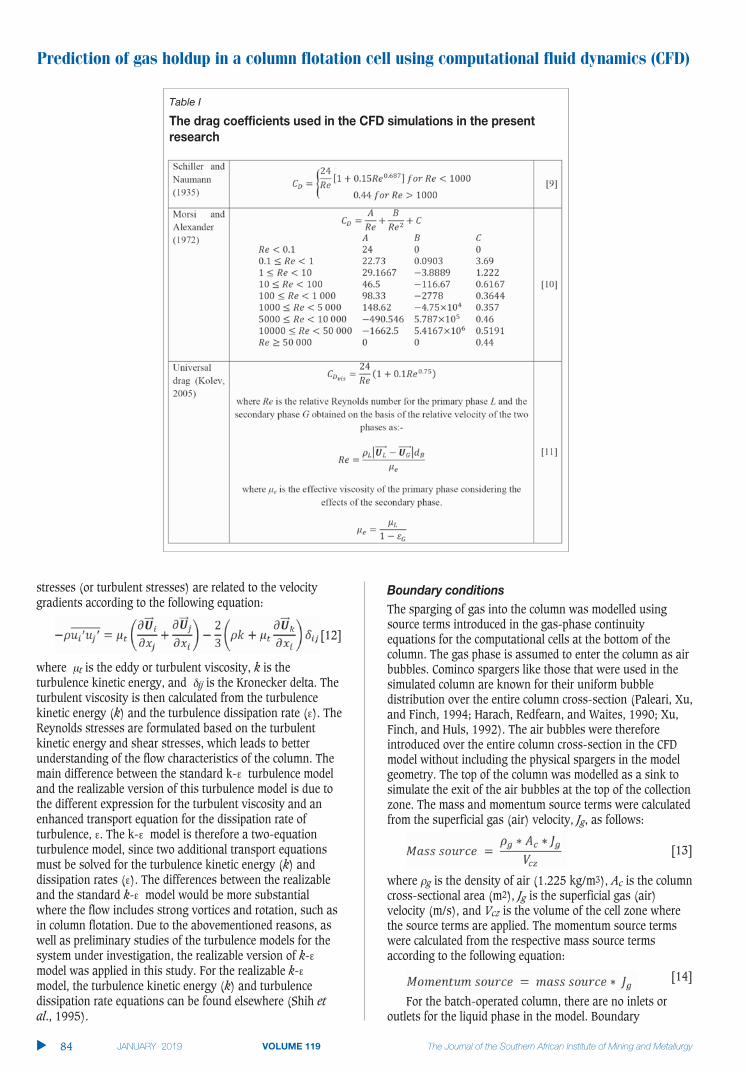
In the present research, simulations were carried out withthree different drag coefficients. The first set of simulationswas performed using the universal drag coefficient (Kolev,2005). Subsequent simulations were conducted with theSchiller-Naumann (Schiller and Naumann, 1935) and Morsi-Alexander (Morsi and Alexander, 1972) drag coefficients inorder to compare the suitability of the three drag models forthe average and axial gas holdup computation in the flotationcolumn. The equations describing the three drag coefficientsare outlined in Table I.

The universal drag coefficient is defined differently forflows that are categorized as either in the viscous regime, thedistorted bubble regime, or the strongly deformed cappedbubbles regime, as determined by the Reynolds number. Atthe moderate superficial gas velocities simulated in thisstudy, the viscous regime conditions apply. The equationpresented in Table I is the one that is applicable when theprevailing flow is in the viscous regime. Further details aboutthe universal drag laws are available in a recent multiphaseflow dynamics book (Kolev, 2005).

Turbulence was modelled using the realizable k-� turbulencemodel (Shih et al., 1995) which is a RANS (Reynolds-Averaged Navier-Stokes) based model. In the RANSmodelling approach, the instantaneous Navier-Stokesequations are replaced with the time-averaged Navier-Stokes(RANS) equations, which are solved to produce a time-averaged flow field. The averaging procedure introducesadditional unknowns; the Reynolds stresses. The Reynoldsstresses are subsequently resolved by employingBoussinesq’s eddy viscosity concept, where the Reynolds


83 �

stresses (or turbulent stresses) are related to the velocitygradients according to the following equation:

[12]

where t is the eddy or turbulent viscosity, k is theturbulence kinetic energy, and ij is the Kronecker delta. Theturbulent viscosity is then calculated from the turbulencekinetic energy (k) and the turbulence dissipation rate ( ). TheReynolds stresses are formulated based on the turbulentkinetic energy and shear stresses, which leads to betterunderstanding of the flow characteristics of the column. Themain difference between the standard k- turbulence modeland the realizable version of this turbulence model is due tothe different expression for the turbulent viscosity and anenhanced transport equation for the dissipation rate ofturbulence, . The k- model is therefore a two-equationturbulence model, since two additional transport equationsmust be solved for the turbulence kinetic energy (k) anddissipation rates ( ). The differences between the realizableand the standard k- model would be more substantialwhere the flow includes strong vortices and rotation, such asin column flotation. Due to the abovementioned reasons, aswell as preliminary studies of the turbulence models for thesystem under investigation, the realizable version of k-model was applied in this study. For the realizable k-model, the turbulence kinetic energy (k) and turbulencedissipation rate equations can be found elsewhere (Shih etal., 1995).

The sparging of gas into the column was modelled usingsource terms introduced in the gas-phase continuityequations for the computational cells at the bottom of thecolumn. The gas phase is assumed to enter the column as airbubbles. Cominco spargers like those that were used in thesimulated column are known for their uniform bubbledistribution over the entire column cross-section (Paleari, Xu,and Finch, 1994; Harach, Redfearn, and Waites, 1990; Xu,Finch, and Huls, 1992). The air bubbles were thereforeintroduced over the entire column cross-section in the CFDmodel without including the physical spargers in the modelgeometry. The top of the column was modelled as a sink tosimulate the exit of the air bubbles at the top of the collectionzone. The mass and momentum source terms were calculatedfrom the superficial gas (air) velocity, Jg, as follows:

[13]

where g is the density of air (1.225 kg/m3), Ac is the columncross-sectional area (m2), Jg is the superficial gas (air)velocity (m/s), and Vcz is the volume of the cell zone wherethe source terms are applied. The momentum source termswere calculated from the respective mass source termsaccording to the following equation:

[14]

For the batch-operated column, there are no inlets oroutlets for the liquid phase in the model. Boundary


�

84

Table I


85 �

conditions were therefore specified for the column wall only.In this case, no slip boundary conditions were applied at thecolumn wall for both the primary phase (water) and thesecondary phase (air bubbles). The application of a sourceterm of the sparger has been proven to be computationallyaffordable; moreover, it helps to introduce the gas bubbles ina uniform fashion across the column. The no-slip boundarycondition for the column walls is a very well-establishedboundary condition that assumes that the fluid has zerovelocity relative to the column wall.

A CFD model (geometry) of this column was subsequentlydeveloped considering the three sections as shown in Figure2. Three-dimensional (3D) simulations of the cylindricalcolumn were then conducted for five different superficial gasvelocities, Jg, from 0.72 to 1.67 cm/s.

The meshing application of ANSYS Workbench was usedto generate the mesh over the model geometry. The meshwas generated using the Sweep method, which creates amesh comprising mainly hexahedral elements. Grid-dependency studies were conducted in order to eliminate thepossibility of errors resulting from an unsuitable mesh size.The mesh was therefore progressively refined from aninitially coarse mesh of cell size equal to 5 cm and number ofcells equal to 97 188 until there were no significant changesin the simulated axial water and bubble velocity profiles.

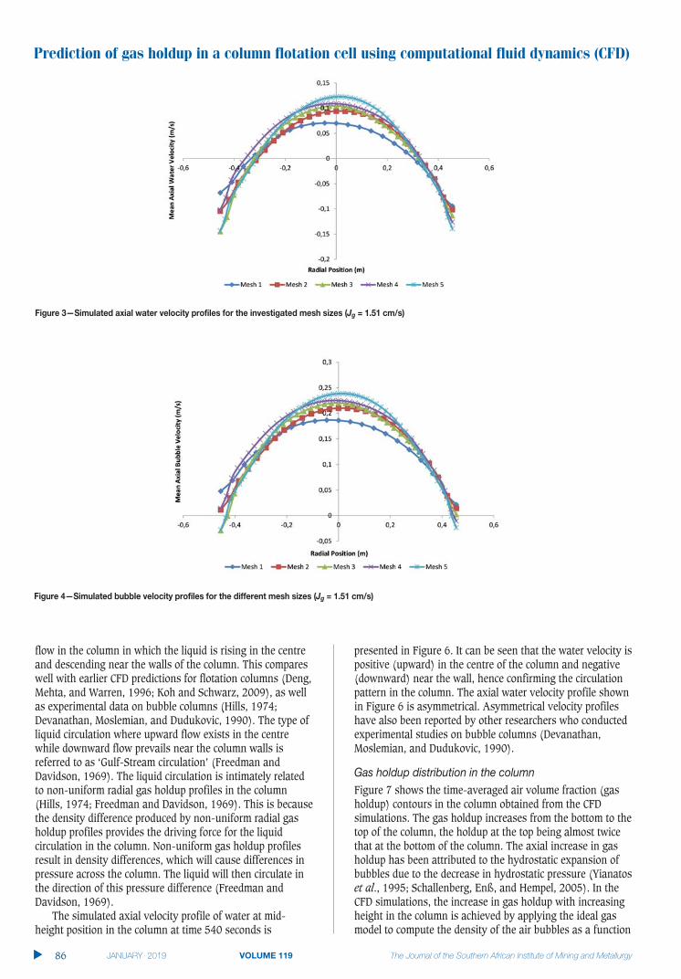
The different mesh sizes that were investigated arepresented in Table II, while the axial velocity profilesobtained for these meshes are shown in Figure 3 and Figure4. It can be seen that the mean axial water and bubblevelocity profiles do not change significantly from mesh 3 upto mesh 5. However, the axial velocity for mesh 5 is slightlyhigher than for mesh 3 and mesh 4. Therefore, based onthese results mesh 4, comprising 884 601 elements with cellsize equal to 2.25 cm, was used for all subsequentsimulations, since it represented a reasonable trade-offbetween the required accuracy and the computational timefor the simulations. A minimum orthogonal quality of 0.840was obtained for the mesh.

Momentum and volume fraction equations were discretizedusing the QUICK scheme, while First Order Upwind wasemployed for turbulence kinetic energy and dissipation ratediscretization. The QUICK scheme provides up to third-orderaccuracy in the computations, while First Order Upwind iseasier to converge. The time step size was 0.05 seconds.

For simulations that were difficult to converge the FirstOrder Upwind scheme was used in place of the QUICK

scheme until convergence. In some of such cases the timestep size was changed from 0.05 seconds to 0.025 seconds toenhance convergence. The simulations were run up to flowtimes of between 400 seconds and 540 seconds since thebubble residence time in a similar sized column wasmeasured at 4–5 minutes (Yianatos et al., 1994).

Two sets of CFD simulations were carried out in this study topredict the average gas holdup and the axial gas holdupvariation in the flotation column. The first set of simulationswas conducted using the universal drag coefficient tocalculate the drag force between the air bubbles and theliquid. Another set of simulations was then performed withthe Schiller-Naumann and the Morsi-Alexander dragcoefficients in order to compare the suitability of the differentdrag models for predicting gas holdup in the column. Thesimulation results obtained with the universal dragcoefficient are presented first, followed by a comparison ofthe results obtained with the three different drag coefficients.

Figure 5 shows the predicted instantaneous velocity vectorsof the liquid (water) at the vertical mid-plane position in thecolumn. The liquid velocity field shows a typical circulating

Table II

Mesh 1 (coarse mesh) 5.00 97 188 106 038Mesh 2 3.75 203 280 218 764Mesh 3 2.70 528 150 555 912Mesh 4 2.25 884 601 925 328Mesh 5 1.85 1 611 132 1 667 575


�

86

flow in the column in which the liquid is rising in the centreand descending near the walls of the column. This compareswell with earlier CFD predictions for flotation columns (Deng,Mehta, and Warren, 1996; Koh and Schwarz, 2009), as wellas experimental data on bubble columns (Hills, 1974;Devanathan, Moslemian, and Dudukovic, 1990). The type ofliquid circulation where upward flow exists in the centrewhile downward flow prevails near the column walls isreferred to as ‘Gulf-Stream circulation’ (Freedman andDavidson, 1969). The liquid circulation is intimately relatedto non-uniform radial gas holdup profiles in the column(Hills, 1974; Freedman and Davidson, 1969). This is becausethe density difference produced by non-uniform radial gasholdup profiles provides the driving force for the liquidcirculation in the column. Non-uniform gas holdup profilesresult in density differences, which will cause differences inpressure across the column. The liquid will then circulate inthe direction of this pressure difference (Freedman andDavidson, 1969).

The simulated axial velocity profile of water at mid-height position in the column at time 540 seconds is

presented in Figure 6. It can be seen that the water velocity ispositive (upward) in the centre of the column and negative(downward) near the wall, hence confirming the circulationpattern in the column. The axial water velocity profile shownin Figure 6 is asymmetrical. Asymmetrical velocity profileshave also been reported by other researchers who conductedexperimental studies on bubble columns (Devanathan,Moslemian, and Dudukovic, 1990).

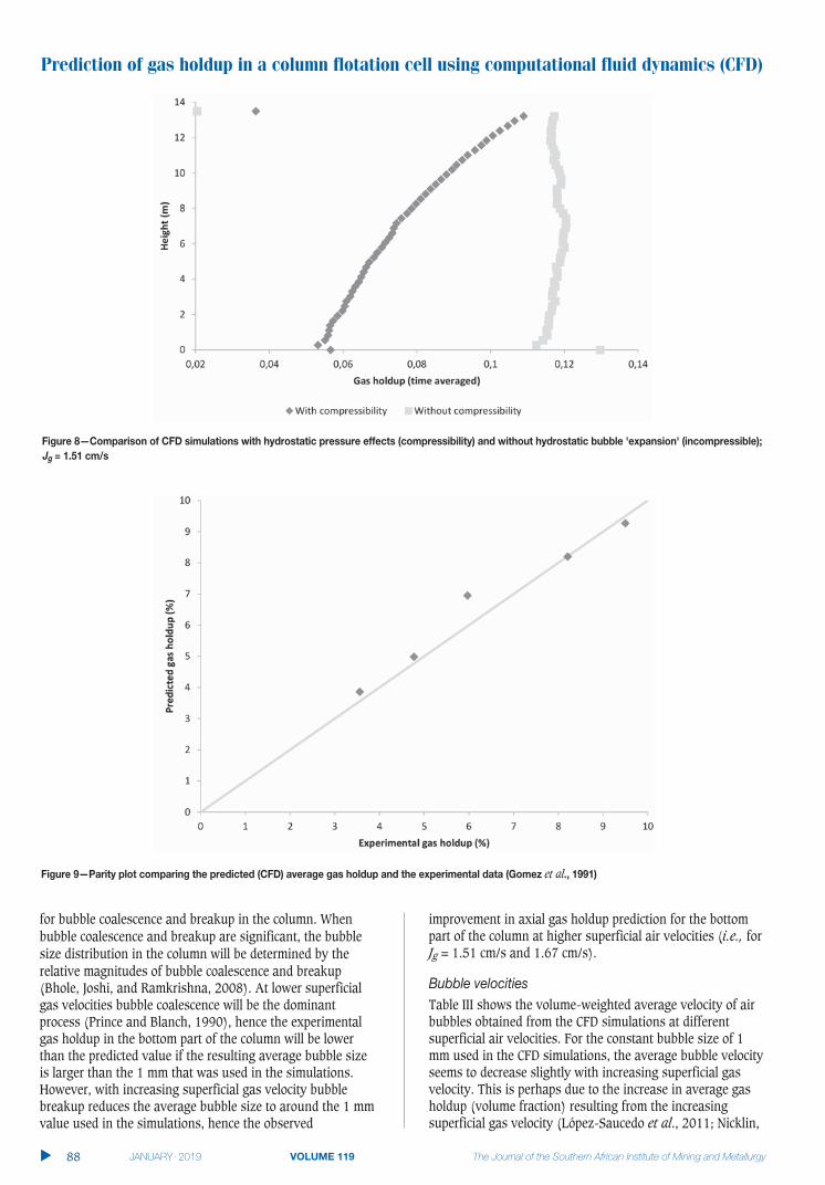
Figure 7 shows the time-averaged air volume fraction (gasholdup) contours in the column obtained from the CFDsimulations. The gas holdup increases from the bottom to thetop of the column, the holdup at the top being almost twicethat at the bottom of the column. The axial increase in gasholdup has been attributed to the hydrostatic expansion ofbubbles due to the decrease in hydrostatic pressure (Yianatoset al., 1995; Schallenberg, Enß, and Hempel, 2005). In theCFD simulations, the increase in gas holdup with increasingheight in the column is achieved by applying the ideal gasmodel to compute the density of the air bubbles as a function

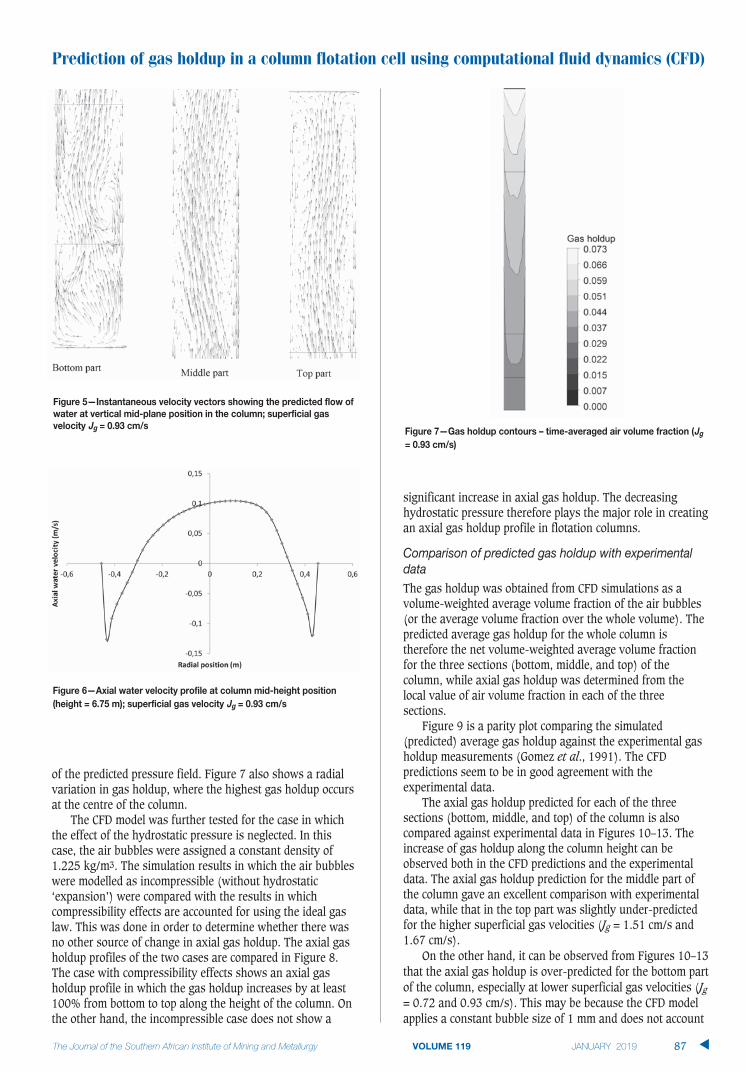
of the predicted pressure field. Figure 7 also shows a radialvariation in gas holdup, where the highest gas holdup occursat the centre of the column.

The CFD model was further tested for the case in whichthe effect of the hydrostatic pressure is neglected. In thiscase, the air bubbles were assigned a constant density of1.225 kg/m3. The simulation results in which the air bubbleswere modelled as incompressible (without hydrostatic‘expansion’) were compared with the results in whichcompressibility effects are accounted for using the ideal gaslaw. This was done in order to determine whether there wasno other source of change in axial gas holdup. The axial gasholdup profiles of the two cases are compared in Figure 8.The case with compressibility effects shows an axial gasholdup profile in which the gas holdup increases by at least100% from bottom to top along the height of the column. Onthe other hand, the incompressible case does not show a

significant increase in axial gas holdup. The decreasinghydrostatic pressure therefore plays the major role in creatingan axial gas holdup profile in flotation columns.

The gas holdup was obtained from CFD simulations as avolume-weighted average volume fraction of the air bubbles(or the average volume fraction over the whole volume). Thepredicted average gas holdup for the whole column istherefore the net volume-weighted average volume fractionfor the three sections (bottom, middle, and top) of thecolumn, while axial gas holdup was determined from thelocal value of air volume fraction in each of the threesections.

Figure 9 is a parity plot comparing the simulated(predicted) average gas holdup against the experimental gasholdup measurements (Gomez et al., 1991). The CFDpredictions seem to be in good agreement with theexperimental data.

The axial gas holdup predicted for each of the threesections (bottom, middle, and top) of the column is alsocompared against experimental data in Figures 10–13. Theincrease of gas holdup along the column height can beobserved both in the CFD predictions and the experimentaldata. The axial gas holdup prediction for the middle part ofthe column gave an excellent comparison with experimentaldata, while that in the top part was slightly under-predictedfor the higher superficial gas velocities (Jg = 1.51 cm/s and1.67 cm/s).

On the other hand, it can be observed from Figures 10–13that the axial gas holdup is over-predicted for the bottom partof the column, especially at lower superficial gas velocities (Jg= 0.72 and 0.93 cm/s). This may be because the CFD modelapplies a constant bubble size of 1 mm and does not account


87 �

Jg

Jg

Jg


for bubble coalescence and breakup in the column. Whenbubble coalescence and breakup are significant, the bubblesize distribution in the column will be determined by therelative magnitudes of bubble coalescence and breakup(Bhole, Joshi, and Ramkrishna, 2008). At lower superficialgas velocities bubble coalescence will be the dominantprocess (Prince and Blanch, 1990), hence the experimentalgas holdup in the bottom part of the column will be lowerthan the predicted value if the resulting average bubble sizeis larger than the 1 mm that was used in the simulations.However, with increasing superficial gas velocity bubblebreakup reduces the average bubble size to around the 1 mmvalue used in the simulations, hence the observed

improvement in axial gas holdup prediction for the bottompart of the column at higher superficial air velocities (i.e., forJg = 1.51 cm/s and 1.67 cm/s).

Table III shows the volume-weighted average velocity of airbubbles obtained from the CFD simulations at differentsuperficial air velocities. For the constant bubble size of 1mm used in the CFD simulations, the average bubble velocityseems to decrease slightly with increasing superficial gasvelocity. This is perhaps due to the increase in average gasholdup (volume fraction) resulting from the increasingsuperficial gas velocity (López-Saucedo et al., 2011; Nicklin,

�

88

et al

Jg

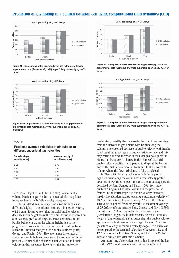
1962; Zhou, Egiebor, and Plitt, L. 1993). When bubblevolume fraction or gas holdup is increased, the drag forceincreases hence the bubble velocity decreases.

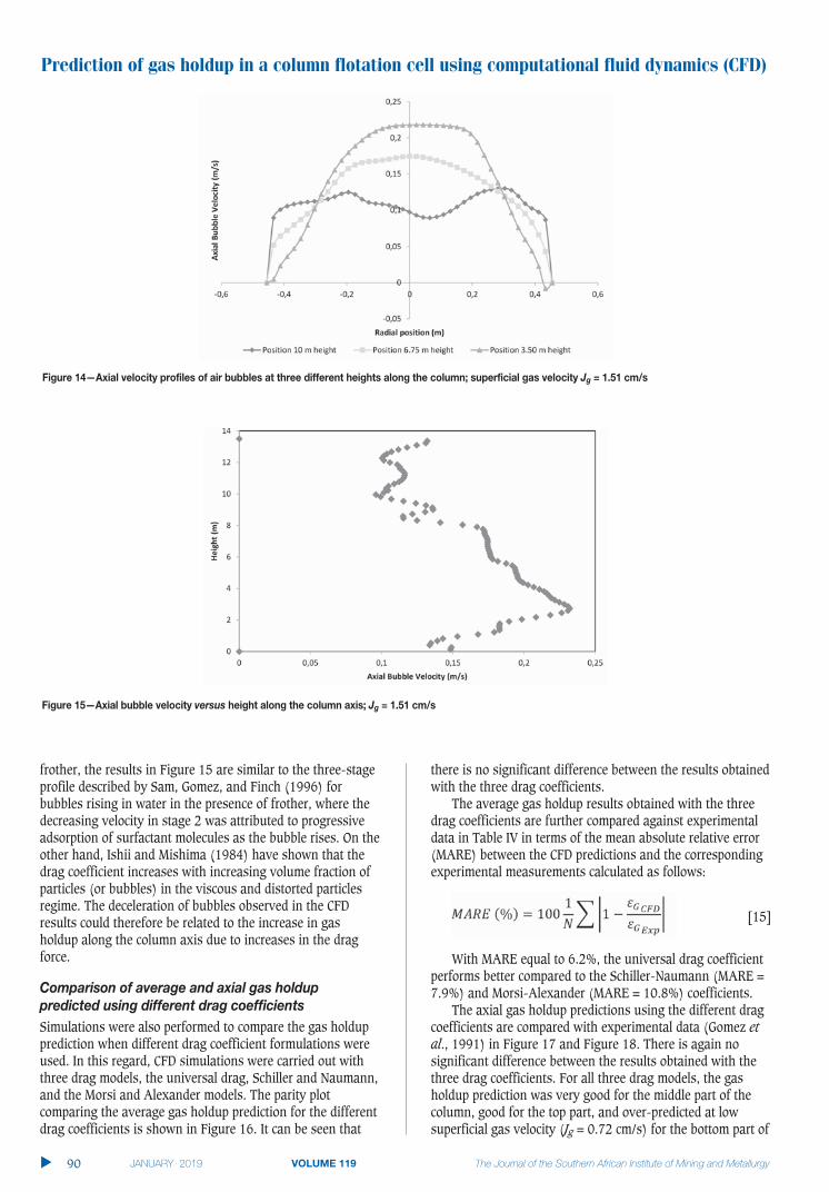
The simulated axial velocity profiles of air bubbles atdifferent heights in the column are shown in Figure 14 for Jg= 1.51 cm/s. It can be seen that the axial bubble velocitydecreases with height along the column. Previous research onaxial velocity profiles of single bubbles identified similarbubble behaviour along the column height due to theprogressive increase in the drag coefficient resulting fromsurfactant-induced changes at the bubble surfaces (Sam,Gomez, and Finch, 1996). However, since the effects ofsurfactants on bubble surfaces are not accounted for in thepresent CFD model, the observed axial variation in bubblevelocity in this case must have its origins in some other

mechanism, possibly the increase in the drag force resultingfrom the increase in gas holdup with height along thecolumn. The observed decrease in bubble velocity with heightcould result in an increase in bubble residence time and thismay cause a further increase in the axial gas holdup profile.Figure 14 also shows a change in the shape of the axialbubble velocity profile from a parabolic shape at the bottomand in the middle to a more uniform profile at the top of thecolumn where the flow turbulence is fully developed.

In Figure 15, the axial velocity of bubbles is plottedagainst height along the column axis. The velocity profileobtained shows three stages, similar to the three-stage profiledescribed by Sam, Gomez, and Finch (1996) for singlebubbles rising in a 4 m water column in the presence offrother. In the initial stage, the bubble velocity increasesrapidly (acceleration stage), reaching a maximum velocity of23.2 cm/s at height of approximately 2.7 m in the column.This value compares favourably with the maximum velocityof 25.0±0.4 cm/s reported by Sam, Gomez, and Finch (1996)for bubbles of 0.9 mm diameter. In the second stage(deceleration stage), the bubble velocity decreases until at aheight of approximately 8.5 m. After that, the bubble velocityappears to fluctuate around an average of about 11.5 cm/s(constant velocity or terminal velocity stage). This value canbe compared to the terminal velocities of between 11.0 and12.0 cm/s observed by Sam, Gomez, and Finch (1996) forsimilar a bubble size (0.9 mm diameter).

An interesting observation here is that in spite of the factthat this CFD model does not account for the effects of


89 �

Table III

0.72 12.790.93 12.331.22 11.781.51 11.841.67 11.61


frother, the results in Figure 15 are similar to the three-stageprofile described by Sam, Gomez, and Finch (1996) forbubbles rising in water in the presence of frother, where thedecreasing velocity in stage 2 was attributed to progressiveadsorption of surfactant molecules as the bubble rises. On theother hand, Ishii and Mishima (1984) have shown that thedrag coefficient increases with increasing volume fraction ofparticles (or bubbles) in the viscous and distorted particlesregime. The deceleration of bubbles observed in the CFDresults could therefore be related to the increase in gasholdup along the column axis due to increases in the dragforce.

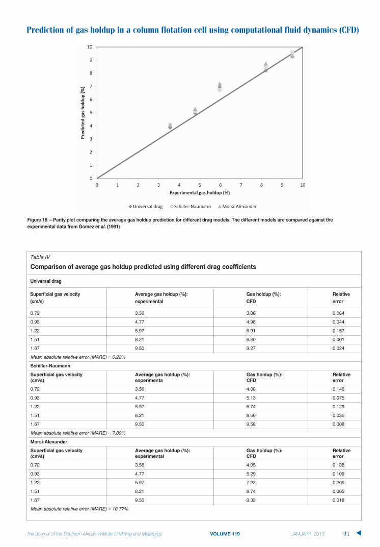
Simulations were also performed to compare the gas holdupprediction when different drag coefficient formulations wereused. In this regard, CFD simulations were carried out withthree drag models, the universal drag, Schiller and Naumann,and the Morsi and Alexander models. The parity plotcomparing the average gas holdup prediction for the differentdrag coefficients is shown in Figure 16. It can be seen that

there is no significant difference between the results obtainedwith the three drag coefficients.

The average gas holdup results obtained with the threedrag coefficients are further compared against experimentaldata in Table IV in terms of the mean absolute relative error(MARE) between the CFD predictions and the correspondingexperimental measurements calculated as follows:

[15]

With MARE equal to 6.2%, the universal drag coefficientperforms better compared to the Schiller-Naumann (MARE =7.9%) and Morsi-Alexander (MARE = 10.8%) coefficients.

The axial gas holdup predictions using the different dragcoefficients are compared with experimental data (Gomez etal., 1991) in Figure 17 and Figure 18. There is again nosignificant difference between the results obtained with thethree drag coefficients. For all three drag models, the gasholdup prediction was very good for the middle part of thecolumn, good for the top part, and over-predicted at lowsuperficial gas velocity (Jg = 0.72 cm/s) for the bottom part of

�

90


91 �

Table IV

0.72 3.56 3.86 0.084

0.93 4.77 4.98 0.044

1.22 5.97 6.91 0.157

1.51 8.21 8.20 0.001

1.67 9.50 9.27 0.024

Mean absolute relative error (MARE) = 6.22%Schiller-Naumann

Superficial gas velocity Average gas holdup (%): Gas holdup (%): Relative

(cm/s) experimenta CFD error

0.72 3.56 4.08 0.146

0.93 4.77 5.13 0.075

1.22 5.97 6.74 0.129

1.51 8.21 8.50 0.035

1.67 9.50 9.58 0.008

Mean absolute relative error (MARE) = 7.89%Morsi-Alexander

Superficial gas velocity Average gas holdup (%): Gas holdup (%): Relative

(cm/s) experimental CFD error

0.72 3.56 4.05 0.138

0.93 4.77 5.29 0.109

1.22 5.97 7.22 0.209

1.51 8.21 8.74 0.065

1.67 9.50 9.33 0.018

Mean absolute relative error (MARE) = 10.77%

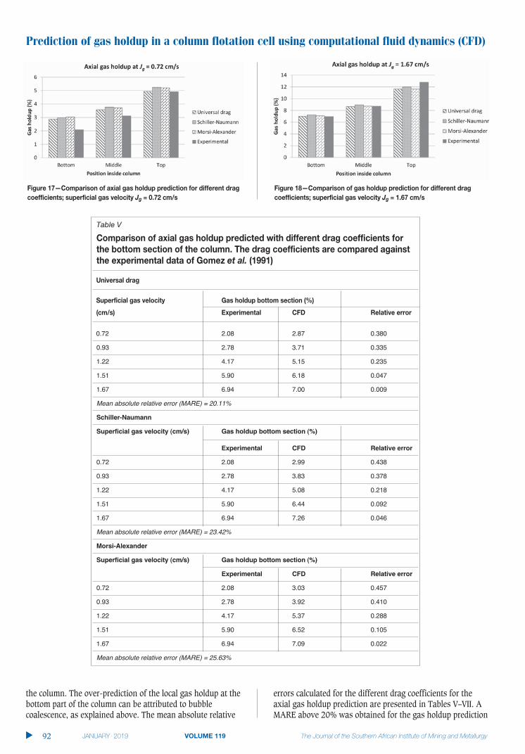
the column. The over-prediction of the local gas holdup at thebottom part of the column can be attributed to bubblecoalescence, as explained above. The mean absolute relative

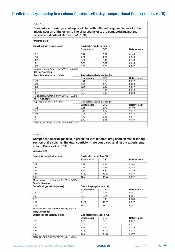
errors calculated for the different drag coefficients for theaxial gas holdup prediction are presented in Tables V–VII. AMARE above 20% was obtained for the gas holdup prediction


�

92

Table V

0.72 2.08 2.87 0.380

0.93 2.78 3.71 0.335

1.22 4.17 5.15 0.235

1.51 5.90 6.18 0.047

1.67 6.94 7.00 0.009


Schiller-Naumann

Superficial gas velocity (cm/s) Gas holdup bottom section (%)

Experimental CFD Relative error

0.72 2.08 2.99 0.438

0.93 2.78 3.83 0.378

1.22 4.17 5.08 0.218

1.51 5.90 6.44 0.092

1.67 6.94 7.26 0.046


Morsi-Alexander

Superficial gas velocity (cm/s) Gas holdup bottom section (%)


0.72 2.08 3.03 0.457

0.93 2.78 3.92 0.410

1.22 4.17 5.37 0.288

1.51 5.90 6.52 0.105

1.67 6.94 7.09 0.022



93 �

Table VI

0.72 3.11 3.57 0.1480.93 4.64 4.61 0.0061.22 5.84 6.44 0.1031.51 7.79 7.67 0.0151.67 8.72 8.66 0.007Mean absolute relative error (MARE) = 5.59%Schiller-Naumann

Superficial gas velocity (cm/s) Gas holdup middle section (%)


0.72 3.11 3.77 0.2120.93 4.64 4.78 0.0301.22 5.84 6.29 0.0771.51 7.79 7.94 0.0191.67 8.72 8.96 0.028Mean absolute relative error (MARE) = 7.32%Morsi-Alexander

Superficial gas velocity (cm/s) Gas holdup middle section (%)


0.72 3.11 3.73 0.1990.93 4.64 4.90 0.0561.22 5.84 6.70 0.1471.51 7.79 8.16 0.0471.67 8.72 8.75 0.003Mean absolute relative error (MARE) = 9.072%

Table VII

et al.

0.72 4.92 4.94 0.0040.93 6.67 6.38 0.0431.22 8.22 8.87 0.0791.51 11.32 10.32 0.0881.67 12.8 11.66 0.089Mean absolute relative error (MARE) = 6.08%Schiller-Naumann

Superficial gas velocity (cm/s) Gas holdup top section (%)


0.72 4.92 5.24 0.0650.93 6.67 6.51 0.0241.22 8.22 8.49 0.0331.51 11.32 10.68 0.0571.67 12.8 12.01 0.062Mean absolute relative error (MARE) = 4.80%Morsi-Alexander

Superficial gas velocity (cm/s) Gas holdup top section (%)


0.72 4.92 5.2 0.0570.93 6.67 6.75 0.0121.22 8.22 9.2 0.1191.51 11.32 11.04 0.0251.67 12.8 11.65 0.090Mean absolute relative error (MARE) = 6.05%


�

94

in the bottom part of the column with all three dragcoefficients. On the other hand, the gas holdup in the middleand top parts of the column was predicted with less than 10%relative error.

CFD modelling was applied to study the gas holdup and itsvariation along the collection zone of a pilot flotation column.Both the predicted average gas holdup and the axial (local)gas holdup were in good agreement with the experimentaldata available in the literature. The generally known gasholdup profile, with the gas holdup values increasing upwardin the column and having maximum values in the centre ofthe column, was also predicted by the CFD simulations.

Three drag models, the universal drag, Schiller-Naumann,and Morsi-Alexander drag coefficients, were compared inorder to determine the suitable drag model for average andaxial gas holdup prediction in the column. The three dragcoefficients all produced good prediction of both the averageand local gas holdup. Therefore, any of these three dragcoefficients can be used to model flotation columnhydrodynamics.

An axial bubble velocity profile was also observed inwhich the bubble velocity magnitude decreased with heightalong the column. The reason for this could be the increase indrag coefficient resulting from the axial increase in gasholdup along the column height. However, the decrease inaxial bubble velocity along the column height can result in afurther increase in the axial gas holdup variations comparedto the effect of the hydrostatic pressure only. The axialvariation in gas holdup could therefore be explained ashaving its origins in two interrelated processes; thehydrostatic expansion of air bubbles and the development ofa bubble velocity profile in which the axial velocity of bubblesdecreases with height along the column.

The authors would like to thank the Nuffic Heart Project, theCopperbelt University, and the Process EngineeringDepartment of Stellenbosch University for providing thefunding and facilities which made this research possible.Computations were performed using the University ofStellenbosch's Rhasatsha High Performance Computing(HPC) cluster.

FD Drag force per unit volume, N/m3

u' Velocity fluctuation, m/s

U Reynolds-averaged velocity, m/s

g Gravitational acceleration, 9.81 m/s2

Ac Column cross-sectional area, m2

CD Drag coefficient, dimensionless

dB Bubble diameter, mm

Jg Superficial gas velocity, cm/s

k Turbulence kinetic energy, m2/s2

P Pressure, Pa

R Universal gas constant

Re Reynolds number, dimensionless

Sq Mass source term for phase q, kg/m3-s

T Temperature

V Volume, m3

H Separation distance for gas holdup measurement

P Pressure difference

T Viscous stress tensor, Pa

G Air volume fraction or gas holdup

k Prandtl number for turbulence kinetic energy,dimensionless

Prandtl number for turbulence energy dissipation rate,dimensionless

Volume fraction

Turbulence dissipation rate, m2/s3

Viscosity, kg/m-s

t Turbulent viscosity, kg/m-s

Density, kg/m3

B BubbleD DragG, g Gasi, j Spatial directionsL Liquidq Phase

BHOLE, M., JOSHI, J., and RAMKRISHNA, D. 2008. CFD simulation of bubble

columns incorporating population balance modeling. Chemical Engineering

Science, vol. 63, no. 8.. pp. 2267–2282.

CHAKRABORTY, D., GUHA, M., and BANERJEE, P. 2009. CFD simulation on influence

of superficial gas velocity, column size, sparger arrangement, and taper

angle on hydrodynamics of the column flotation cell. Chemical

Engineering Communications, vol. 196, no. 9. pp. 1102–1116.

CHEN, J., YANG, N., GE, W., and LI, J. 2009. Computational fluid dynamics

simulation of regime transition in bubble columns incorporating the dual-

bubble-size model. Industrial & Engineering Chemistry Research vol. 48,

no. 17. p. 8172–8179.

CHEN, P., DUDUKOVI , M., and SANYAL, J. 2005. Three dimensional simulation of

bubble column flows with bubble coalescence and breakup. AIChE Journal,

vol. 51, no. 3. pp. 696–712.

CHEN, P., SANYAL, J., and DUDUKOVIC, M. 2004. CFD modeling of bubble columns

flows: Implementation of population balance. Chemical Engineering

Science, vol. 59, no. 22. pp. 5201–5207.

DELNOIJ. E., KUIPERS. J.A.M., and VAN SWAAIJ. W.P.M. 1997. Computational fluid

dynamics applied to gas-liquid contactors. Chemical Engineering Science,

vol. 52, no. 21–22, pp. 3623-3368.

DENG, H., MEHTA, R., and WARREN, G. 1996. Numerical modeling of flows in

flotation columns. International Journal of Mineral Processing, vol. 48,

no. 1. pp, 61–72.

DEVANATHAN, N., MOSLEMIAN, D., and DUDUKOVIC, M. 1990. Flow mapping in

bubble columns using CARPT. Chemical Engineering Science, vol. 45,

no. 8. pp. 2285–2291.

DOBBY, G., AMELUNXEN, R., and FINCH, J. 1985. Column flotation: Some plant

experience and model development. Proceedings of the IFAC Symposium

on Automation for Mineral Development, Brisbane. Norris, A.W., and

Rurner, D.R. (eds). Australasian Institute of Mining and Metallurgy,

Melbourne. pp. 259–264.

FINCH, J.A. and DOBBY, G.S. 1990. Column Flotation. Pergamon Press, Oxford

UK.

FINCH, J. and HARDIE, C. 1999. An example of innovation from the waste

management industry: Deinking flotation cells. Minerals Engineering, vol.

12, no. 5. pp. 467–475.

FREEDMAN, W. and DAVIDSON, J. 1969. Hold-up and liquid circulation in bubble

columns. Transactions of the Institution of Chemical Engineers and the

Chemical Engineer, vol. 47, no. 8. pp, T251–T262.

GAL-OR, B. and WASLO, S. 1968. Hydrodynamics of an ensemble of drops (or

bubbles) in the presence or absence of surfactants. Chemical Engineering

Science, vol. 23, no. 12. pp. 1431–1446.

GOMEZ, C., URIBE-SALAS, A., FINCH, J., and HULS, B. 1991. Gas holdup

measurement in flotation columns using electrical conductivity. Canadian

Metallurgical Quarterly, vol. 30, no. 4. pp. 201–205.

GOMEZ, C., URIBE-SALAS, A., FINCH, J., and HULS, B. 1995. Axial gas holdup

profiles in the collection zones of flotation columns. Minerals and

Metallurgical Processing, vol. 12, no. 1. pp. 16–23.

HARACH, P.L., REDFEARN, M.A., and WAITES, D.B. 1990 Sparging system for

column flotation. US patent 4,911,826. Cominco Ltd.

HERNANDEZ, H., GOMEZ, C., and FINCH, J. 2003. Gas dispersion and de-inking in a

flotation column. Minerals Engineering, vol. 16, no. 8. pp. 739–744.

HILLS, J. 1974. Radial non-uniformity of velocity and voidage in a bubble

column. Tranactions of the Institution of Chemical Enginering, vol. 52,

no. 1. pp. 1–9.

ISHII, M. and MISHIMA, K. 1984. Two-fluid model and hydrodynamic constitutive

relations. Nuclear Engineering and Design, vol. 82, no. 2. pp. 107–126.

KOH, P. and SCHWARZ, M. 2009. CFD models of microcel and Jameson flotation

cells. Proceedings of the Seventh International Conference on CFD in the

Minerals and Process Industries, CSIRO, Melbourne, Australia. CSIRO.

KOH, P., SCHWARZ, M., ZHU, Y., BOURKE, P., PEAKER, R., and FRANZIDIS, J. 2003.:

Development of CFD models of mineral flotation cells. Proceedings of the

Third International Conference on Computational Fluid Dynamics in the

Minerals and Process Industries, Melbourne, Australia. Witt, P.J. and

Schwarz, M.P. (eds). CSIRO, Australia. pp. 171–175.

KOLEV, N.I. 2005. Multiphase Flow Dynamics. Vol. 2 Thermal and Mechanical

Interactions. 2nd edn. Springer, Berlin.

LEICHTLE, G.F. 1998. Analysis of bubble generating devices in a deinking

column. MEng thesis, McGill University.

LÓPEZ-SAUCEDO, F., URIBE-SALAS, A., PÉREZ-GARIBAY, R., MAGALLANES-HERNÁNDEZ

L, and LARA-VALENZUELA C. 2011. Modelling of bubble size in industrial

flotation columns. Canadian Metallurgical Quarterly, vol. 50, no. 2.

pp. 95–101.

LÓPEZ-SAUCEDO, F., URIBE-SALAS, A., PÉREZ-GARIBAY, R., and MAGALLANES-

HERNÁNDEZ, L. 2012. Gas dispersion in column flotation and its effect on

recovery and grade. Canadian Metallurgical Quarterly, vol. 51, no. 2. pp.

11–17.

MASSINAEI, M., KOLAHDOOZAN, M., NOAPARAST M., OLIAZADEH, M., YIANATOS, J.,

SHAMSADINI, R., and YARAHMADID, M. 2009. Hydrodynamic and kinetic

characterization of industrial columns in rougher circuit. Minerals

Engineering, vol. 22, no. 4. pp. 357–365.

MICHELE. V. and HEMPEL, D.C. 2002. Liquid flow and phase holdup—

measurement and CFD modeling for two-and three-phase bubble columns.

Chemical Engineering Science, vol. 57, no. 11. pp. 1899-1908.

MORSI, S. and ALEXANDER, 1972. An investigation of particle trajectories in two-

phase flow systems. Journal of Fluid Mechanics, vol. 55, no. 2.

pp. 193–208.

NICKLIN, D. 1962. Two-phase bubble flow. Chemical Engineering Science, vol.

17, no. 9. pp. 693–702.

PALEARI, F., XU, M., and FINCH, J. 1994. Radial gas holdup profiles: The

influence of sparger systems. Minerals and Metallurgical Processing, vol.

11, no. 2. pp. 111–117.

PFLEGER, D. and BECKER, S. 2001. Modelling and simulation of the dynamic flow

behaviour in a bubble column. Chemical Engineering Science, vol. 56, no.

4. pp. 1737–47.

PFLEGER, D., GOMES S., GILBERT, N., and WAGNER, H. 1999. Hydrodynamic

simulations of laboratory scale bubble columns fundamental studies of the

Eulerian–Eulerian modelling approach. Chemical Engineering Science, vol.

54, no. 21. pp. 5091–5099.

PRINCE, M.J. and BLANCH, H.W. 1990. Bubble coalescence and break up in

air sparged bubble columns. AIChE Journal, vol. 36, no. 10.

pp. 1485–1499.

SAM, A., GOMEZ, C., and FINCH, J. 1996. Axial velocity profiles of single bubbles

in water/frother solutions. International Journal of Mineral Processing,

vol. 47, no. 3. pp. 177–196.

SCHALLENBERG, J., ENß, J.H., and HEMPEL, D.C. 2005. The important role of local

dispersed phase hold-ups for the calculation of three-phase bubble

columns. Chemical Engineering Science, vol. 60, no. 22. pp. 6027–6033.

SCHILLER, L. and NAUMANN, A. 1935. A drag coefficient correlation. Vdi Zeitung.

vol. 77. pp. 318–20.

SHIH, T., LIOU, W.W., SHABBIR, A., YANG, Z., and ZHU, J. 1995. A new k- eddy

viscosity model for high Reynolds number turbulent flows. Computers &

Fluids, vol. 24, no. 3. pp. 227–238.

TAVERA, F., ESCUDERO, R., and FINCH, J. 2001. Gas holdup in flotation columns:

Laboratory measurements. International Journal of Mineral Processing,

vol. 61, no. 1. pp. 23–40.

XU, M., FINCH, J., and HULS, B. 1992. Measurement of radial gas holdup profiles

in a flotation column. International Journal of Mineral Processing, vol. 36,

no. 3. pp. 229–244.

YIANATOS, J., BERGH, L., DURÁN, O., DIAZ, F., and HERESI, N. 1994. Measurement

of residence time distribution of the gas phase in flotation columns.

Minerals Engineering, vol. 7, no. 2. pp. 333–344.

YIANATOS, J., BERGH, L., SEPULVEDA, C., and NÚÑEZ, R. 1995. Measurement of

axial pressure profiles in large-size industrial flotation columns. Minerals

Engineering, vol. 8, no. 1. pp. 101–109.

ZHOU, Z, EGIEBOR, N., and PLITT, L. 1993. Frother effects on bubble motion in a

swarm. Canadian Metallurgical Quarterly, vol. 32, no. 2. pp. 89–96.

ZHOU, Z. and EGIEBOR, N. 1993. Prediction of axial gas holdup profiles in

flotation columns. Minerals Engineering. vol. 6, no. 3. pp. 307–312.

ZHOU, Z., EGIEBOR, N., and PLITT, L. 1993. Frother effects on bubble motion in a

swarm. Canadian Metallurgical Quarterly, vol. 32, no. 2. pp. 89–96. �


95 �

Documents

Prediction of gas holdup in a column flotation cell using … · 2019-03-07 · Prediction of gas holdup in a column flotation cell using computational fluid dynamics (CFD) 2009;