Embed Size (px)
Citation preview
Contents lists available at ScienceDirect
Journal of the Mechanics and Physics of Solids
Journal of the Mechanics and Physics of Solids 59 (2011) 297–319
0022-50
doi:10.1
n Corr
E-m
journal homepage: www.elsevier.com/locate/jmps
Predicting variability in the dynamic failure strength of brittlematerials considering pre-existing flaws
Nitin P. Daphalapurkar a,n, K.T. Ramesh a, Lori Graham-Brady b, Jean-Francois Molinari c
a The Johns Hopkins University, Department of Mechanical Engineering, Baltimore, MD 21218, USAb The Johns Hopkins University, Department of Civil Engineering, Baltimore, MD 21218, USAc L.S.M.S.—I.I.S.—E.N.A.C., Ecole Polytechnique Federale de Lausanne, 1015, Lausanne, Switzerland
a r t i c l e i n f o
Article history:
Received 13 June 2010
Received in revised form
2 October 2010
Accepted 24 October 2010Available online 30 October 2010
Keywords:
Dynamic strengths
Finite element method
Flaw distributions
Brittle failure
Crack interactions
96/$ - see front matter & 2010 Elsevier Ltd. A
016/j.jmps.2010.10.006
esponding author. Tel.: +1 410 516 8781; fax
ail address: [email protected] (N.P. Daphalapurka
a b s t r a c t
We perform two-dimensional dynamic fracture simulations of a specimen in biaxial
tension, incorporating various distributions of pre-existing microcracks. The simulations
consider the spatial distribution of flaws while modeling the discrete failure processes of
crack interactions and coalescence, and predict the macroscopic variability in failure
strength. The model quantitatively predicts the effect (on the dynamic failure strength) of
different shapes of the flaw size distribution function, the random spatial distribution of
flaws, and the random local resistance to crack growth (i.e. strength) associated with each
flaw. The effect of changing material volumes on the variability in failure strengths is also
examined in relation to the flaw size distribution. The effect of loading rate on the
variability in failure strengths is presented in a form that will enable improved
constitutive modeling using non-local formulations at the continuum scale.
& 2010 Elsevier Ltd. All rights reserved.
1. Introduction and background
Brittle materials such as ceramics have low toughness and are very sensitive to processing-related defects (we will refer tothese as flaws). Flaw size distributions have been known for many years to lead to variability in the quasistatic strength ofbrittle materials. This strength variability is normally accounted for through a weakest link approach such as that of Weibull(1939), and the distribution of quasistatic strength has been associated with the internal flaw size distribution by Jayatilakaand Trustrum (1977). However, the influence of the flaw size distribution on the dynamic compressive response of brittlematerials has been shown by Paliwal and Ramesh (2008) to be much more complex than described by Weibull-typeapproaches because of the competition between flaw activation, the dynamics of crack growth, and the rate of loading. Thispaper seeks to address the influence of these intrinsic flaw size distributions on the variability in the dynamic failure strengthin tension.
The physical nature of the typical flaw distribution in a model ceramic (sintered aluminum nitride, AlN) is presented, forexample, in Fig. 1. There are several different types of flaws that are present at various length scales, as shown in the scanningelectron micrographs of typical fracture surfaces in this material. At the smallest scale of interest, Fig. 1a shows thepolycrystalline nature of the ceramic with an average grain size of about 6 mm. The lighter phase seen between the AlN grainsin this micrograph is yttrium oxide (Y2O3), which is a sintering agent used to help densify the polycrystalline material duringthe sintering process. This ‘‘interphase’’ material leads to variability in the grain boundary strengths, and these boundariescan present sites for crack nucleation and paths for crack growth (note the generally intergranular nature of the fracture
ll rights reserved.
: + 1 410 516 4316.
r).
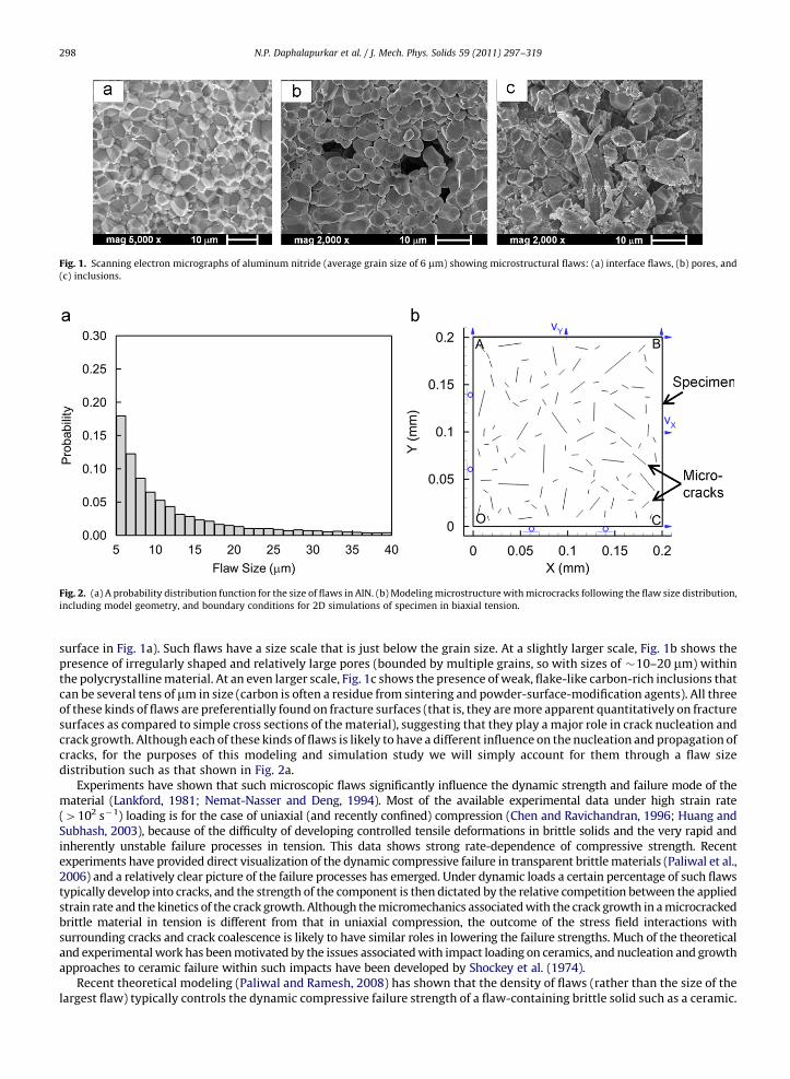
Fig. 1. Scanning electron micrographs of aluminum nitride (average grain size of 6 mm) showing microstructural flaws: (a) interface flaws, (b) pores, and
(c) inclusions.
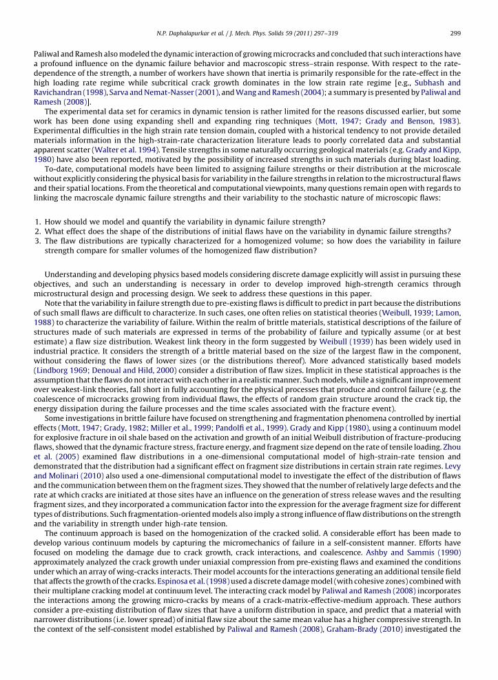
Fig. 2. (a) A probability distribution function for the size of flaws in AlN. (b) Modeling microstructure with microcracks following the flaw size distribution,
including model geometry, and boundary conditions for 2D simulations of specimen in biaxial tension.
N.P. Daphalapurkar et al. / J. Mech. Phys. Solids 59 (2011) 297–319298
surface in Fig. 1a). Such flaws have a size scale that is just below the grain size. At a slightly larger scale, Fig. 1b shows thepresence of irregularly shaped and relatively large pores (bounded by multiple grains, so with sizes of �10–20 mm) withinthe polycrystalline material. At an even larger scale, Fig. 1c shows the presence of weak, flake-like carbon-rich inclusions thatcan be several tens of mm in size (carbon is often a residue from sintering and powder-surface-modification agents). All threeof these kinds of flaws are preferentially found on fracture surfaces (that is, they are more apparent quantitatively on fracturesurfaces as compared to simple cross sections of the material), suggesting that they play a major role in crack nucleation andcrack growth. Although each of these kinds of flaws is likely to have a different influence on the nucleation and propagation ofcracks, for the purposes of this modeling and simulation study we will simply account for them through a flaw sizedistribution such as that shown in Fig. 2a.
Experiments have shown that such microscopic flaws significantly influence the dynamic strength and failure mode of thematerial (Lankford, 1981; Nemat-Nasser and Deng, 1994). Most of the available experimental data under high strain rate(4102 s�1) loading is for the case of uniaxial (and recently confined) compression (Chen and Ravichandran, 1996; Huang andSubhash, 2003), because of the difficulty of developing controlled tensile deformations in brittle solids and the very rapid andinherently unstable failure processes in tension. This data shows strong rate-dependence of compressive strength. Recentexperiments have provided direct visualization of the dynamic compressive failure in transparent brittle materials (Paliwal et al.,2006) and a relatively clear picture of the failure processes has emerged. Under dynamic loads a certain percentage of such flawstypically develop into cracks, and the strength of the component is then dictated by the relative competition between the appliedstrain rate and the kinetics of the crack growth. Although the micromechanics associated with the crack growth in a microcrackedbrittle material in tension is different from that in uniaxial compression, the outcome of the stress field interactions withsurrounding cracks and crack coalescence is likely to have similar roles in lowering the failure strengths. Much of the theoreticaland experimental work has been motivated by the issues associated with impact loading on ceramics, and nucleation and growthapproaches to ceramic failure within such impacts have been developed by Shockey et al. (1974).
Recent theoretical modeling (Paliwal and Ramesh, 2008) has shown that the density of flaws (rather than the size of thelargest flaw) typically controls the dynamic compressive failure strength of a flaw-containing brittle solid such as a ceramic.
N.P. Daphalapurkar et al. / J. Mech. Phys. Solids 59 (2011) 297–319 299
Paliwal and Ramesh also modeled the dynamic interaction of growing microcracks and concluded that such interactions havea profound influence on the dynamic failure behavior and macroscopic stress–strain response. With respect to the rate-dependence of the strength, a number of workers have shown that inertia is primarily responsible for the rate-effect in thehigh loading rate regime while subcritical crack growth dominates in the low strain rate regime [e.g., Subhash andRavichandran (1998), Sarva and Nemat-Nasser (2001), and Wang and Ramesh (2004); a summary is presented by Paliwal andRamesh (2008)].
The experimental data set for ceramics in dynamic tension is rather limited for the reasons discussed earlier, but somework has been done using expanding shell and expanding ring techniques (Mott, 1947; Grady and Benson, 1983).Experimental difficulties in the high strain rate tension domain, coupled with a historical tendency to not provide detailedmaterials information in the high-strain-rate characterization literature leads to poorly correlated data and substantialapparent scatter (Walter et al. 1994). Tensile strengths in some naturally occurring geological materials (e.g. Grady and Kipp,1980) have also been reported, motivated by the possibility of increased strengths in such materials during blast loading.
To-date, computational models have been limited to assigning failure strengths or their distribution at the microscalewithout explicitly considering the physical basis for variability in the failure strengths in relation to the microstructural flawsand their spatial locations. From the theoretical and computational viewpoints, many questions remain open with regards tolinking the macroscale dynamic failure strengths and their variability to the stochastic nature of microscopic flaws:
1.
How should we model and quantify the variability in dynamic failure strength? 2. What effect does the shape of the distributions of initial flaws have on the variability in dynamic failure strengths? 3. The flaw distributions are typically characterized for a homogenized volume; so how does the variability in failurestrength compare for smaller volumes of the homogenized flaw distribution?
Understanding and developing physics based models considering discrete damage explicitly will assist in pursuing theseobjectives, and such an understanding is necessary in order to develop improved high-strength ceramics throughmicrostructural design and processing design. We seek to address these questions in this paper.
Note that the variability in failure strength due to pre-existing flaws is difficult to predict in part because the distributionsof such small flaws are difficult to characterize. In such cases, one often relies on statistical theories (Weibull, 1939; Lamon,1988) to characterize the variability of failure. Within the realm of brittle materials, statistical descriptions of the failure ofstructures made of such materials are expressed in terms of the probability of failure and typically assume (or at bestestimate) a flaw size distribution. Weakest link theory in the form suggested by Weibull (1939) has been widely used inindustrial practice. It considers the strength of a brittle material based on the size of the largest flaw in the component,without considering the flaws of lower sizes (or the distributions thereof). More advanced statistically based models(Lindborg 1969; Denoual and Hild, 2000) consider a distribution of flaw sizes. Implicit in these statistical approaches is theassumption that the flaws do not interact with each other in a realistic manner. Such models, while a significant improvementover weakest-link theories, fall short in fully accounting for the physical processes that produce and control failure (e.g. thecoalescence of microcracks growing from individual flaws, the effects of random grain structure around the crack tip, theenergy dissipation during the failure processes and the time scales associated with the fracture event).
Some investigations in brittle failure have focused on strengthening and fragmentation phenomena controlled by inertialeffects (Mott, 1947; Grady, 1982; Miller et al., 1999; Pandolfi et al., 1999). Grady and Kipp (1980), using a continuum modelfor explosive fracture in oil shale based on the activation and growth of an initial Weibull distribution of fracture-producingflaws, showed that the dynamic fracture stress, fracture energy, and fragment size depend on the rate of tensile loading. Zhouet al. (2005) examined flaw distributions in a one-dimensional computational model of high-strain-rate tension anddemonstrated that the distribution had a significant effect on fragment size distributions in certain strain rate regimes. Levyand Molinari (2010) also used a one-dimensional computational model to investigate the effect of the distribution of flawsand the communication between them on the fragment sizes. They showed that the number of relatively large defects and therate at which cracks are initiated at those sites have an influence on the generation of stress release waves and the resultingfragment sizes, and they incorporated a communication factor into the expression for the average fragment size for differenttypes of distributions. Such fragmentation-oriented models also imply a strong influence of flaw distributions on the strengthand the variability in strength under high-rate tension.
The continuum approach is based on the homogenization of the cracked solid. A considerable effort has been made todevelop various continuum models by capturing the micromechanics of failure in a self-consistent manner. Efforts havefocused on modeling the damage due to crack growth, crack interactions, and coalescence. Ashby and Sammis (1990)approximately analyzed the crack growth under uniaxial compression from pre-existing flaws and examined the conditionsunder which an array of wing-cracks interacts. Their model accounts for the interactions generating an additional tensile fieldthat affects the growth of the cracks. Espinosa et al. (1998) used a discrete damage model (with cohesive zones) combined withtheir multiplane cracking model at continuum level. The interacting crack model by Paliwal and Ramesh (2008) incorporatesthe interactions among the growing micro-cracks by means of a crack-matrix-effective-medium approach. These authorsconsider a pre-existing distribution of flaw sizes that have a uniform distribution in space, and predict that a material withnarrower distributions (i.e. lower spread) of initial flaw size about the same mean value has a higher compressive strength. Inthe context of the self-consistent model established by Paliwal and Ramesh (2008), Graham-Brady (2010) investigated the
N.P. Daphalapurkar et al. / J. Mech. Phys. Solids 59 (2011) 297–319300
variability of dynamic uniaxial compressive strength resulting from random spatial and size distributions of flaws, andprovides a significant improvement over the weakest-link theory.
While the models described above account for random flaw sizes and strengths, they are not able to explicitly representthe microstructure. A body of recent literature has developed explicit microstructure-based models. For example, due to thecomplexity of the dynamic fracture problem, computations explicitly considering a grain-level analysis have providedinsights into a number of phenomena. Zavattieri and Espinosa (2001) demonstrated crack initiation and propagation at theinterface for brittle materials with material failure dominated by intergranular cracking. To capture the stochasticityassociated with the microfracture process they used predefined cohesive elements at the boundaries, which werecharacterized by a Weibull distribution of interfacial strengths. Their analyses showed that a detailed modeling of grainmorphology is required in order to capture the damage kinetics. Maiti et al. (2005) used a similar scheme (assumingintergranular crack propagation) to carry out mesoscale analyses of fragmentation of ceramics under tension. They reportedthat the average grain size influences the final damage in the material, and has an effect on the average fragment size at highloading rates. Kraft et al. (2008) used dynamic insertion of cohesive zones at the grain boundaries of the polycrystallinemicrostructure to investigate the effect of microcrack density on the failure strength in compression. The strengths obtainedwere a realization of the random flaw size and spatial distribution, and their results captured the general trend of increasingfailure strengths with decreasing flaw density. Overall, the results from grain level analyses demonstrate that an additionallength scale is required to capture the characteristics of damage evolution. However, the computational expense associatedwith these models makes it difficult to incorporate measures of resulting strength and variability.
In order to simplify such explicit microstructural models, approaches using cohesive zone models have used a distributionof cohesive strengths representing flaw distributions rather than carrying out the entire grain-level analysis to understandsensitivity of parameters (e.g. Srolovitz and Beale, 1988). Often, cohesive strengths based on the macroscopic tensilestrengths are assigned to the microstructure. The spatial locations having relatively weak cohesive strengths (within thedistribution) then affect the way in which the cracks nucleate, propagate and coalesce, leading to variability in failurestrengths (Denoual and Hild, 2000). Models by Zhou and Molinari (2004) and Brannon et al. (2007) take into account materialheterogeneities in the microstructure by assigning smeared mechanical properties.
In this paper, we couple the statistical nature of flaw distributions with dynamic failure mechanics simulations tounderstand strength variability in a model brittle material. Simulations are performed by explicitly incorporating various flawdistributions through pre-defined microcracks to obtain macroscopic variability in failure strength (similar to Zhou andMolinari, 2004; Zhou and Molinari, 2005). Both flaw size distributions and spatial distributions of flaws are accounted for in theanalyses. A bounded Pareto distribution function and a 4-parameter Weibull distribution function are used to modeldistributions of flaw sizes and length scale dependent cohesive strengths, respectively, while their spatial distribution israndomly assigned. Note that we keep the flaw density the same, the effect of this having been studied in the work of Graham-Brady (2010). The dynamic failure process is simulated through activation of microcracks and their growth within the(initially) pristine material. The paper is organized as follows: Section 2 describes the procedure used to create modelmicrostructures incorporating flaw distributions. Section 3 describes the computational model. Section 4 presents typicalsimulation results and discussions, followed by a summary of the major conclusions.
2. Incorporating flaw distributions
The statistical nature of macroscopic strengths in brittle materials can be traced to the flaws at the microstructural level, andwe will model these as initial microcracks in a pristine material, as shown in Fig. 2b. The approach here considers two differentstatistical influences that contribute to the mechanical behavior of the overall material: (a) the size distribution and spatialdistribution of flaws and (b) the length scale dependent microscopic properties of the pristine material (the material between theflaws in Fig. 2b). The first of these can be obtained by means of physical examination of microstructures and fracture surfaces suchas those shown in Fig. 1. The second of these is based on the physical argument that the definition of the pristine material requiresthe definition of a representative volume element (with the size on the order of the spacing between flaws), and that the subscalemicrostructure of the material will result in length scale dependent mechanical properties for the pristine material, due forinstance to finite grain size distributions and sampling thereof. We discuss each of these influences in what follows.
With respect to the first of these influences, for the example case of AlN, we can estimate the probability of occurrences offlaws based on a large number (200) of SEM images such as those in Fig. 1. This tells us that the density of interface relatedflaws is the largest, followed by the flaw densities of the pores and then the relatively low probability of finding inclusions.We will refer to the flaw density as the combined densities of all the flaws. The overall flaw density is on the order of107–1010 m�2 for this specific material. Based on the limits of characterization instruments at the high end and simulationcapabilities on the low end, we bound the distribution in the range 5–40 mm. The different types of flaws occurring in theceramics are treated as equivalent microcracks in the simulations presented herein. The flaw size distribution is typically(Trustrum and Jayatilaka, 1983) represented using a distribution function which decays like an inverse power law function(Fig. 2a). We use a bounded version of the Pareto distribution function to describe the probability density of flaw sizes. We willrefer to the characteristic probability distribution function of the flaw sizes as g(s, k), described using
gðs,kÞ ¼kLks�k�1
1�ðL=HÞk, ð1Þ
N.P. Daphalapurkar et al. / J. Mech. Phys. Solids 59 (2011) 297–319 301
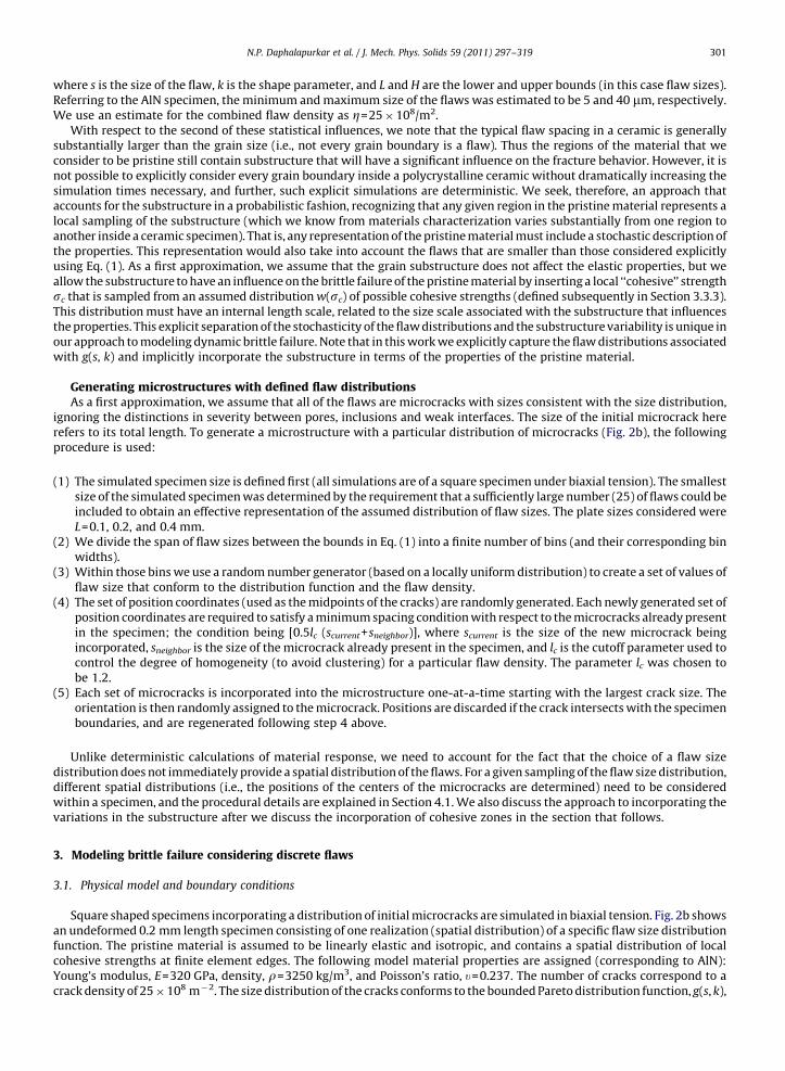
where s is the size of the flaw, k is the shape parameter, and L and H are the lower and upper bounds (in this case flaw sizes).Referring to the AlN specimen, the minimum and maximum size of the flaws was estimated to be 5 and 40 mm, respectively.We use an estimate for the combined flaw density as Z=25�108/m2.
With respect to the second of these statistical influences, we note that the typical flaw spacing in a ceramic is generallysubstantially larger than the grain size (i.e., not every grain boundary is a flaw). Thus the regions of the material that weconsider to be pristine still contain substructure that will have a significant influence on the fracture behavior. However, it isnot possible to explicitly consider every grain boundary inside a polycrystalline ceramic without dramatically increasing thesimulation times necessary, and further, such explicit simulations are deterministic. We seek, therefore, an approach thataccounts for the substructure in a probabilistic fashion, recognizing that any given region in the pristine material represents alocal sampling of the substructure (which we know from materials characterization varies substantially from one region toanother inside a ceramic specimen). That is, any representation of the pristine material must include a stochastic description ofthe properties. This representation would also take into account the flaws that are smaller than those considered explicitlyusing Eq. (1). As a first approximation, we assume that the grain substructure does not affect the elastic properties, but weallow the substructure to have an influence on the brittle failure of the pristine material by inserting a local ‘‘cohesive’’ strengthsc that is sampled from an assumed distribution w(sc) of possible cohesive strengths (defined subsequently in Section 3.3.3).This distribution must have an internal length scale, related to the size scale associated with the substructure that influencesthe properties. This explicit separation of the stochasticity of the flaw distributions and the substructure variability is unique inour approach to modeling dynamic brittle failure. Note that in this work we explicitly capture the flaw distributions associatedwith g(s, k) and implicitly incorporate the substructure in terms of the properties of the pristine material.
Generating microstructures with defined flaw distributionsAs a first approximation, we assume that all of the flaws are microcracks with sizes consistent with the size distribution,
ignoring the distinctions in severity between pores, inclusions and weak interfaces. The size of the initial microcrack hererefers to its total length. To generate a microstructure with a particular distribution of microcracks (Fig. 2b), the followingprocedure is used:
(1)
The simulated specimen size is defined first (all simulations are of a square specimen under biaxial tension). The smallestsize of the simulated specimen was determined by the requirement that a sufficiently large number (25) of flaws could beincluded to obtain an effective representation of the assumed distribution of flaw sizes. The plate sizes considered wereL=0.1, 0.2, and 0.4 mm.(2)
We divide the span of flaw sizes between the bounds in Eq. (1) into a finite number of bins (and their corresponding binwidths).(3)
Within those bins we use a random number generator (based on a locally uniform distribution) to create a set of values offlaw size that conform to the distribution function and the flaw density.(4)
The set of position coordinates (used as the midpoints of the cracks) are randomly generated. Each newly generated set ofposition coordinates are required to satisfy a minimum spacing condition with respect to the microcracks already presentin the specimen; the condition being [0.5lc (scurrent+sneighbor)], where scurrent is the size of the new microcrack beingincorporated, sneighbor is the size of the microcrack already present in the specimen, and lc is the cutoff parameter used tocontrol the degree of homogeneity (to avoid clustering) for a particular flaw density. The parameter lc was chosen tobe 1.2.(5)
Each set of microcracks is incorporated into the microstructure one-at-a-time starting with the largest crack size. Theorientation is then randomly assigned to the microcrack. Positions are discarded if the crack intersects with the specimenboundaries, and are regenerated following step 4 above.Unlike deterministic calculations of material response, we need to account for the fact that the choice of a flaw sizedistribution does not immediately provide a spatial distribution of the flaws. For a given sampling of the flaw size distribution,different spatial distributions (i.e., the positions of the centers of the microcracks are determined) need to be consideredwithin a specimen, and the procedural details are explained in Section 4.1. We also discuss the approach to incorporating thevariations in the substructure after we discuss the incorporation of cohesive zones in the section that follows.
3. Modeling brittle failure considering discrete flaws
3.1. Physical model and boundary conditions
Square shaped specimens incorporating a distribution of initial microcracks are simulated in biaxial tension. Fig. 2b showsan undeformed 0.2 mm length specimen consisting of one realization (spatial distribution) of a specific flaw size distributionfunction. The pristine material is assumed to be linearly elastic and isotropic, and contains a spatial distribution of localcohesive strengths at finite element edges. The following model material properties are assigned (corresponding to AlN):Young’s modulus, E=320 GPa, density, r=3250 kg/m3, and Poisson’s ratio, u=0.237. The number of cracks correspond to acrack density of 25�108 m�2. The size distribution of the cracks conforms to the bounded Pareto distribution function, g(s, k),
N.P. Daphalapurkar et al. / J. Mech. Phys. Solids 59 (2011) 297–319302
with the shape parameter k=1, which we will designate as g(s, 1). The initial microcracks are discretized using cohesiveelements (described in the next section).
Zero displacement boundary conditions are applied for nodes on edge OA along the X degree of freedom, and nodes onedge OC along the Y degree of freedom. The displacement of point O is thus constrained along the X as well as the Y degrees offreedom. Constant velocity boundary conditions are applied, (0, vy) on edge AB and (vx, 0) on edge BC. Here vx and vy arecomponents of velocities along X and Y, with vx ¼ L_e and vy ¼ L_e, where L is the original length of the specimen, and _e is thenominal strain rate. In this study we apply an initial velocity field which corresponds to an initial uniform strain rate andavoids the issue of interactions of the initial loading wave with the crack tips. The components of the initial velocity field (onall the nodes) are: vx ¼ x_e and vy ¼ y_e, where x and y are the components of the position vector of a node with respect to theorigin (at point O). The stable time step used in our simulations for an average mesh size of 1.25 mm is 2.2 ps, and satisfactorilyresolves the time scales (discussed in the next section) associated with the cohesive law.
3.2. Finite element method
Consider a general case of a body in its reference configuration in Euclidean space B0CR3 corresponding to time t0. Itsmotion can be described by a displacement field, u(X,t) corresponding to time t. Equations of dynamic equilibrium areenforced using the weak form of linear momentum balance as follows:Z
B0
P : r0vdV0þ
ZB0
r0bUvdV0þ
Z@B0t
te : r0vdS0�
ZB0
r0€uUvdV0 ¼ 0 ð2Þ
where P is the first Piola–Kirchoff stress, r0 is the material gradient, r0 is the mass density, b are the body forces, €u is theacceleration, te and uðX,tÞ are the prescribed tractions and displacement on boundaries qB0t and qB0u, respectively, such thatqB0u\qB0t=|. In addition, v is an admissible virtual displacement satisfying boundary conditions on qB0t. The symbol ‘:’ heredenotes an inner product between tensors and the superimposed dots on u denote the material time derivative. Eq. (2)implies that the work done by internal forces and external work is balanced by the inertial virtual work.
Discrete discontinuities are modeled explicitly using interfaces by introducing a jump condition which satisfiesZS0
tcU½½v��dS0 ð3Þ
where ½½v�� represents a displacement jump across an interface, located at S0, and tc is the cohesive traction. The weak form ofthe principle of virtual work is thenZ
B0
P : r0vdV0þ
ZB0
r0bUvdV0þ
Z@B0
te : r0vdS0�
ZB0
r0aUv dV0�
ZS0
tcU ½v�½ �dS0 ¼ 0 ð4Þ
In the finite element method (FEM), a discretized version of Eq. (3) is solved, which is
MaþRintðxÞ ¼ Rext
ðtÞ ð5Þ
where M is a lumped mass matrix, a is the nodal acceleration, Rext and Rint are the external and internal forces, and x is thenodal coordinate. We use a Newmark’s scheme (see Belytschko, 1983; Hughes, 1987) of integration over time and second-order accurate explicit version to determine the solution of the problem. The finite elements use quadratic shape functions.The time step used for this explicit time-marching scheme is based on Courant–Friedrichs–Lewy condition for convergence as
Dtstablera lec
� �ð6Þ
where c is the dilatational wave speed based on material properties, le is the smallest element size out of the discretized bodyB0, and a is a factor whose value is 0.1 or less. The factor a is necessary in cohesive element simulations so that the simulationscan progressively travel through the linearly decreasing curve of the cohesive law, and it ensures numerical stability.
3.3. Modeling crack growth
We view the modeling of crack growth under tensile loading as amounting to capturing the crack-tip process zone in termsof a phenomenological traction-separation model (a cohesive zone model). We implement this in terms of a cohesive modelfor crack growth within the pristine material, with the dynamic insertion of cohesive elements based on a stochasticapproximation of the subgrid physics, as described in the previous section.
3.3.1. Cohesive zone model
The essential feature of implementing a cohesive zone into numerical analysis is the cohesive element (red dashed line inFig. 3a), which simulates the crack-tip process zone. In a cohesive element, the material separation is governed by thecohesive law which defines the relation between crack surface traction and opening displacement. We use the mixed-modecohesive model developed by Camacho and Ortiz (1996), and Pandolfi et al. (1999), accounting for tension-shear coupling.
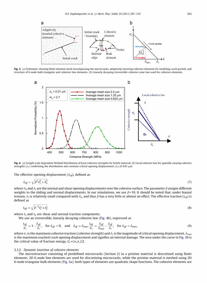
Fig. 3. (a) Schematic showing finite element mesh encompassing the microcracks, adaptively inserting cohesive elements for modeling crack growth, and
structure of 6-node bulk triangular and cohesive line elements. (b) Linearly decaying irreversible cohesive zone law used for cohesive elements.
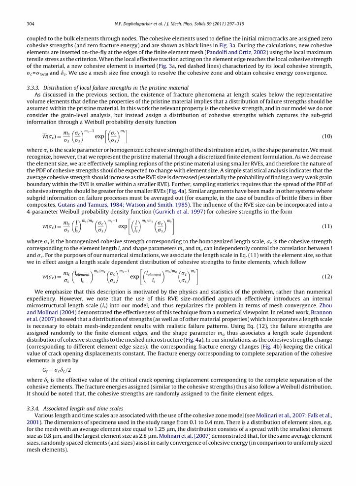
Fig. 4. (a) Length scale dependent Weibull distribution of local cohesive strengths for brittle material. (b) Local cohesive law for spatially varying cohesive
strengths (sc) confirming the distribution and constant critical opening displacement (dc) of 0.01 mm.
N.P. Daphalapurkar et al. / J. Mech. Phys. Solids 59 (2011) 297–319 303
The effective opening displacement (deff), defined as
deff ¼
ffiffiffiffiffiffiffiffiffiffiffiffiffiffiffiffiffiffiffiffib2d2
s þd2n
qð7Þ
where dn and ds are the normal and shear opening displacements over the cohesive surface. The parameter b assigns differentweights to the sliding and normal displacements. In our simulations, we use b=10. It should be noted that, under biaxialtension, ds is relatively small compared with dn, and thus b has a very little or almost no effect. The effective traction (teff) isdefined as
teff ¼
ffiffiffiffiffiffiffiffiffiffiffiffiffiffiffiffiffiffiffiffiffib�2t2
s þt2n
qð8Þ
where ts and tn are shear and normal traction components.We use an irreversible, linearly decaying cohesive law (Fig. 4b), expressed as
teff
sc¼ 1�
deff
dc, for deff 40, and deff ¼ dmax,
teff
sc¼
deff
dmax�deff
dc, for deff odmax, ð9Þ
wheresc is the maximum cohesive traction (cohesive strength) and dc is the magnitude of critical opening displacement. dmax
is the maximum reached crack opening displacement and signifies an internal damage. The area under the curve in Fig. 3b isthe critical value of fracture energy, Gc=(scdc)/2.
3.3.2. Dynamic insertion of cohesive elements
The microstructure consisting of predefined microcracks (Section 2) in a pristine material is discretized using finiteelements. 2D 6-node line elements are used for discretizing microcracks, while the pristine material is meshed using 2D6-node triangular bulk elements (Fig. 3a); both types of elements use quadratic shape functions. The cohesive elements are
N.P. Daphalapurkar et al. / J. Mech. Phys. Solids 59 (2011) 297–319304
coupled to the bulk elements through nodes. The cohesive elements used to define the initial microcracks are assigned zerocohesive strengths (and zero fracture energy) and are shown as black lines in Fig. 3a. During the calculations, new cohesiveelements are inserted on-the-fly at the edges of the finite element mesh (Pandolfi and Ortiz, 2002) using the local maximumtensile stress as the criterion. When the local effective traction acting on the element edge reaches the local cohesive strengthof the material, a new cohesive element is inserted (Fig. 3a, red dashed lines) characterized by its local cohesive strength,sc=slocal and dc. We use a mesh size fine enough to resolve the cohesive zone and obtain cohesive energy convergence.
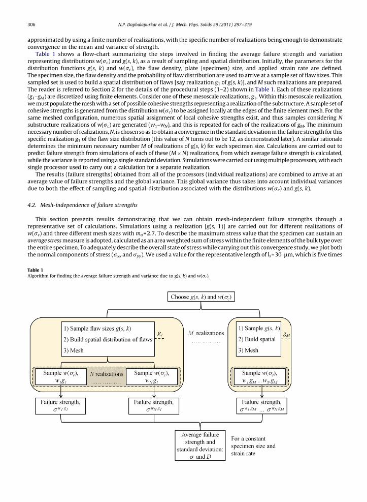
3.3.3. Distribution of local failure strengths in the pristine material
As discussed in the previous section, the existence of fracture phenomena at length scales below the representativevolume elements that define the properties of the pristine material implies that a distribution of failure strengths should beassumed within the pristine material. In this work the relevant property is the cohesive strength, and in our model we do notconsider the grain-level analysis, but instead assign a distribution of cohesive strengths which captures the sub-gridinformation through a Weibull probability density function
wðscÞ ¼ms
ss
sc
ss
� �ms�1
expsc
ss
� �ms� �
ð10Þ
wheress is the scale parameter or homogenized cohesive strength of the distribution and ms is the shape parameter. We mustrecognize, however, that we represent the pristine material through a discretized finite element formulation. As we decreasethe element size, we are effectively sampling regions of the pristine material using smaller RVEs, and therefore the nature ofthe PDF of cohesive strengths should be expected to change with element size. A simple statistical analysis indicates that theaverage cohesive strength should increase as the RVE size is decreased (essentially the probability of finding a very weak grainboundary within the RVE is smaller within a smaller RVE). Further, sampling statistics requires that the spread of the PDF ofcohesive strengths should be greater for the smaller RVEs (Fig. 4a). Similar arguments have been made in other systems wheresubgrid information on failure processes must be averaged out (for example, in the case of bundles of brittle fibers in fibercomposites, Gutans and Tamuzs, 1984; Watson and Smith, 1985). The influence of the RVE size can be incorporated into a4-parameter Weibull probability density function (Gurvich et al. 1997) for cohesive strengths in the form
wðscÞ ¼ms
ss
l
ls
� �ms=ma sc
ss
� �ms�1
expl
ls
� �ms=ma sc
ss
� �ms" #
ð11Þ
where ss is the homogenized cohesive strength corresponding to the homogenized length scale, sc is the cohesive strengthcorresponding to the element length l, and shape parameters ms and ma can independently control the correlation between l
and sc. For the purposes of our numerical simulations, we associate the length scale in Eq. (11) with the element size, so thatwe in effect assign a length scale dependent distribution of cohesive strengths to finite elements, which follow
wðscÞ ¼ms
ss
lelement
ls
� �ms=ma sc
ss
� �ms�1
explelement
ls
� �ms=ma sc
ss
� �ms" #
ð12Þ
We emphasize that this description is motivated by the physics and statistics of the problem, rather than numericalexpediency. However, we note that the use of this RVE size-modified approach effectively introduces an internalmicrostructural length scale (ls) into our model, and thus regularizes the problem in terms of mesh convergence. Zhouand Molinari (2004) demonstrated the effectiveness of this technique from a numerical viewpoint. In related work, Brannonet al. (2007) showed that a distribution of strengths (as well as of other material properties) which incorporates a length scaleis necessary to obtain mesh-independent results with realistic failure patterns. Using Eq. (12), the failure strengths areassigned randomly to the finite element edges, and the shape parameter ma thus associates a length scale dependentdistribution of cohesive strengths to the meshed microstructure (Fig. 4a). In our simulations, as the cohesive strengths change(corresponding to different element edge sizes); the corresponding fracture energy changes (Fig. 4b) keeping the criticalvalue of crack opening displacements constant. The fracture energy corresponding to complete separation of the cohesiveelements is given by
Gc ¼ scdc=2
where dc is the effective value of the critical crack opening displacement corresponding to the complete separation of thecohesive elements. The fracture energies assigned (similar to the cohesive strengths) thus also follow a Weibull distribution.It should be noted that, the cohesive strengths are randomly assigned to the finite element edges.
3.3.4. Associated length and time scales
Various length and time scales are associated with the use of the cohesive zone model (see Molinari et al., 2007; Falk et al.,2001). The dimensions of specimens used in the study range from 0.1 to 0.4 mm. There is a distribution of element sizes, e.g.for the mesh with an average element size equal to 1.25 mm, the distribution consists of a spread with the smallest elementsize as 0.8 mm, and the largest element size as 2.8 mm. Molinari et al. (2007) demonstrated that, for the same average elementsizes, randomly spaced elements (and sizes) assist in early convergence of cohesive energy (in comparison to uniformly sizedmesh elements).
N.P. Daphalapurkar et al. / J. Mech. Phys. Solids 59 (2011) 297–319 305
For the type of cohesive law considered, where the failure stress varies linearly within the cohesive zone, the length of theprocess zone ahead of a stationary crack was estimated by Palmer and Rice (1973) to be
lz ¼9p32
KIC
sc
� �2
ð13Þ
where for plane strain conditions
KIC ¼E
1�n2Gc
� �1=2
ð14Þ
Note that this process zone size decreases for a dynamically propagating crack (Broberg, 1999); we do not attempt tocapture this latter behavior. Numerical studies carried out by Kraft et al. (2008) indicate that at least two cohesive elementscharacterized by a quadratic shape function are required to resolve the cohesive zone and to obtain convergence ofmacroscopic failure stresses, and we satisfy this condition. The finite elements used in our simulations thus satisfactorilyresolve the cohesive zone sizes associated with the distribution of cohesive strengths, and this will be demonstrated in theresults section.
Kraft et al. (2008) investigated the toughness controlled regime of macroscopic failure strengths of an edge crackedspecimen for different ratios of cohesive zone length (at zero crack-tip velocity) to specimen length, and arrived at a criticalratio of 1/20 above which there is a gradually increasing tendency for strength controlled fracture. Our specimen sizesconform to this condition in terms of the ratio. Note that for simulations considered in this work which incorporate adistribution of flaws, the interaction of specimen boundaries with the microcrack cohesive zones located near the edge of theplate is not precluded, and is physical (Kraft et al., 2008).
An investigation of the effects of high rate of loading demands examination of various time scales in the simulation. Thereare two time scales associated with the cohesive interfaces. The first is the response time associated with the cohesive law,and is given by (Camacho and Ortiz, 1996; Molinari et al., 2007)
t0 ¼E
c
Gc
s2c
ð15Þ
The variable t0 is an intrinsic material parameter that determines whether an applied strain rate is perceived as a low orhigh strain rate by the cohesive interface during the crack opening process.
The corresponding characteristic strain rate (Molinari et al., 2007) is
_e0 ¼sc=E
t0ð16Þ
Another time scale is associated with the time required for complete decohesion of the cohesive law and is extrinsic in thatit takes into account the rate-of-deformation
tc ¼dc
c _e
� �1=2
ð17Þ
where _e is the applied strain rate and dc is the critical crack opening displacement. The stable time step used in oursimulations is able to resolve this time-scale.
4. Results and discussion
4.1. Stochastic nature associated with the spatial distribution
We will refer to the terms sampling (of a distribution function) and spatial-distribution (associated with the sampledpopulation) for the local failure strength (sc) and the flaw size (s). The probability density functions for each of thesequantities, w(sc) and g(s, k) are described in Sections 3.3.3 and 2, respectively. Sampling is the process of selecting a subset ofvalues (e.g. a finite subset of flaw sizes) within a larger representative population (e.g., a continuous distribution of flaw sizes).Once the sampling has been performed, each of the individual values has a spatial location within the specimen randomlyassigned to them (e.g. cohesive strengths are randomly assigned to the edges of the finite element mesh, while the centers ofthe microcracks are randomly placed within the dimensions of the specimen). A realization is a specific configuration of thespecimen with a specific set of spatial locations assigned to the individual elements (e.g. flaw sizes) in a specific sampled set. Itis apparent that there are infinitely many possible realizations of a specimen of a given material (i.e., once a specimen size ischosen for a material with a specified attribute distribution, there are infinitely many possible realizations of the specimenthat satisfy the specified probability distributions). This is analogous to the idea that there are infinitely many possiblespecimens one might cut out of an infinitely large block of material, with each specimen consisting of a different sampling,both in spatial location and size, of the distribution of flaws. However, presumably all of these specimens (realizations) havesomething in common—they represent the material in some way. For example, the specimens will have a distribution ofstrengths that correspond in some way to their internal structure. Our interest is in characterizing this distribution ofstrengths, and we choose to do so in terms of a representative average strength and a variance in strength. This is
N.P. Daphalapurkar et al. / J. Mech. Phys. Solids 59 (2011) 297–319306
approximated by using a finite number of realizations, with the specific number of realizations being enough to demonstrateconvergence in the mean and variance of strength.
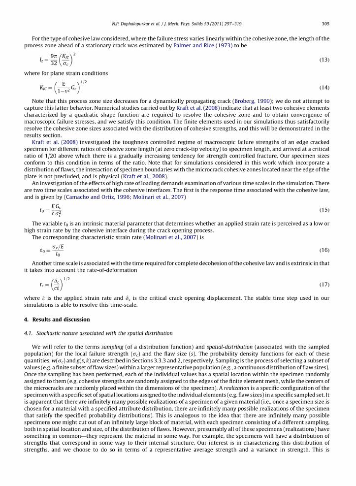
Table 1 shows a flow-chart summarizing the steps involved in finding the average failure strength and variationrepresenting distributions w(sc) and g(s, k), as a result of sampling and spatial distribution. Initially, the parameters for thedistribution functions g(s, k) and w(sc), the flaw density, plate (specimen) size, and applied strain rate are defined.The specimen size, the flaw density and the probability of flaw distribution are used to arrive at a sample set of flaw sizes. Thissampled set is used to build a spatial distribution of flaws [say realization g1 of g(s, k)], and M such realizations are prepared.The reader is referred to Section 2 for the details of the procedural steps (1–2) shown in Table 1. Each of these realizations(g1–gM) are discretized using finite elements. Consider one of these mesoscale realizations, g1. Within this mesoscale realization,we must populate the mesh with a set of possible cohesive strengths representing a realization of the substructure. A sample set ofcohesive strengths is generated from the distribution w(sc) to be assigned locally at the edges of the finite element mesh. For thesame meshed configuration, numerous spatial assignment of local cohesive strengths exist, and thus samples considering N
substructure realizations of w(sc) are generated (w1–wN), and this is repeated for each of the realizations of gM. The minimumnecessary number of realizations, N, is chosen so as to obtain a convergence in the standard deviation in the failure strength for thisspecific realization g1 of the flaw size distribution (this value of N turns out to be 12, as demonstrated later). A similar rationaledetermines the minimum necessary number M of realizations of g(s, k) for each specimen size. Calculations are carried out topredict failure strength from simulations of each of these (M�N) realizations, from which average failure strength is calculated,while the variance is reported using a single standard deviation. Simulations were carried out using multiple processors, with eachsingle processor used to carry out a calculation for a separate realization.
The results (failure strengths) obtained from all of the processors (individual realizations) are combined to arrive at anaverage value of failure strengths and the global variance. This global variance thus takes into account individual variancesdue to both the effect of sampling and spatial-distribution associated with the distributions w(sc) and g(s, k).
4.2. Mesh-independence of failure strengths
This section presents results demonstrating that we can obtain mesh-independent failure strengths through arepresentative set of calculations. Simulations using a realization [g(s, 1)] are carried out for different realizations ofw(sc) and three different mesh sizes with ma=2.7. To describe the maximum stress value that the specimen can sustain anaverage stress measure is adopted, calculated as an area weighted sum of stress within the finite elements of the bulk type overthe entire specimen. To adequately describe the overall state of stress while carrying out this convergence study, we plot boththe normal components of stress (sxx and syy). We used a value for the representative length of ls=30 mm, which is five times
Table 1Algorithm for finding the average failure strength and variance due to g(s, k) and w(sc).
N.P. Daphalapurkar et al. / J. Mech. Phys. Solids 59 (2011) 297–319 307
the average grain size (to obtain homogenization). The critical values of crack-opening displacement (dc) and homogenizedstress (ss) were chosen as 0.01 mm and 200 MPa, respectively. Fig. 4a shows the probability distribution of cohesive strengthsbeing assigned at the microstructural level at a length scale corresponding to the size of the finite element. For the finiteelements in a particular average mesh size the critical value of crack opening displacement is kept constant, and the cohesivestrengths have a spatial variation, illustrated schematically in Fig. 4b. As a consequence there is a spatial distribution of Gc
being assigned. The average length of cohesive zone in our simulations is 5 mm (ranges from 3.75 to 6 mm). An average meshsize of 1.25 mm satisfactorily resolves the cohesive zone lengths (with two or more quadratic elements in each case, Kraftet al., 2008). Fig. 4a shows the different distributions of cohesive strengths automatically assigned for three different sizes offinite element mesh using this approach. The average value of cohesive strength being assigned is 610 MPa. Note that in oursimulations the ratio of size of the specimen to the cohesive zone length is generally greater than 20 (Kraft et al., 2008). Wedefine convergence for a set of results from a particular mesh size if the average value and standard-deviation of peak stressescompared with one finer mesh-size are within an acceptable limit (4% in this work). The results presented for convergence ofpeak stress and cohesive energy were carried out for biaxial tension loading under a constant strain rate of 105/s. Fig. A1aand b, in the Appendix, shows convergence in average peak stress value and cohesive energy for three different mesh sizes,demonstrating converged results for an average mesh size of 1.25 mm. This mesh size and the corresponding mesh sizemodification factor (ma=2.7) are kept constant in the simulation results that follow.
4.3. Representative result for a specimen under biaxial tension
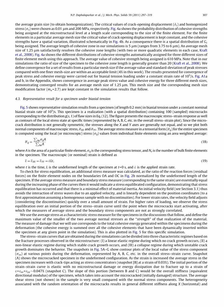
Fig. 5 shows representative simulation results from a specimen (of length 0.2 mm) in biaxial tension under a constant nominalbiaxial strain rate of 105/s. This specimen is a realization (with a spatial distribution) containing 100 (sampled) microcrackscorresponding to the distribution g(s, 1) of flaw sizes in Eq. (12). The figure presents the macroscopic stress–strain response as wellas contours of the local stress state at specific times (represented by A, B, C, etc. in the overall stress–strain plot). Since the micro-crack distribution is not generally symmetric, the stresses along the X and Y axes are generally not equal, and so we plot bothnormal components of macroscopic stress,sXX andsYY . The average stress measure in a tensorial form (sij) for the entire specimenis computed using the local (or microscopic) stress (sij) values from individual finite elements using an area weighted average:
s ij ¼
PNesijAP
NeAð18Þ
where A is the area of a particular finite element,sij is the corresponding stress tensor, and Ne is the number of bulk finite elementsin the specimen. The macroscopic (or nominal) strain is defined as
e ¼ eXX ¼ eYY ¼ _eLt, ð19Þ
where t is the time, L is the undeformed length of the specimen at t=0 s, and _e is the applied strain rate.To check for stress equilibration, an additional stress measure was calculated, as the ratio of the reaction forces (residual
forces) on the finite element nodes on the boundaries OA and OC in Fig. 2b normalized by the undeformed length of thespecimen. If the average stress measure and boundary stress measure (corresponding to the same strain) are essentially equalduring the increasing phase of the curves then it would indicate a stress equilibrated configuration, demonstrating that stressequilibration has occurred and that there is a minimal effect of material inertia. An initial velocity field (see Section 3.1) thusavoids the interaction of stress waves due to an applied velocity, and is linearly dependent on the position coordinates (to afirst approximation assuming a homogenous sample with no discontinuities). For lower strain rates, the velocity field adjusts(considering the discontinuities) quickly over a small amount of strain. For higher rates of loading, we observe the stressequilibration over an initial portion of the stress–strain curve until the point when the microcracks start activating, afterwhich the measures of average stress and the boundary stress components are not as strongly correlated.
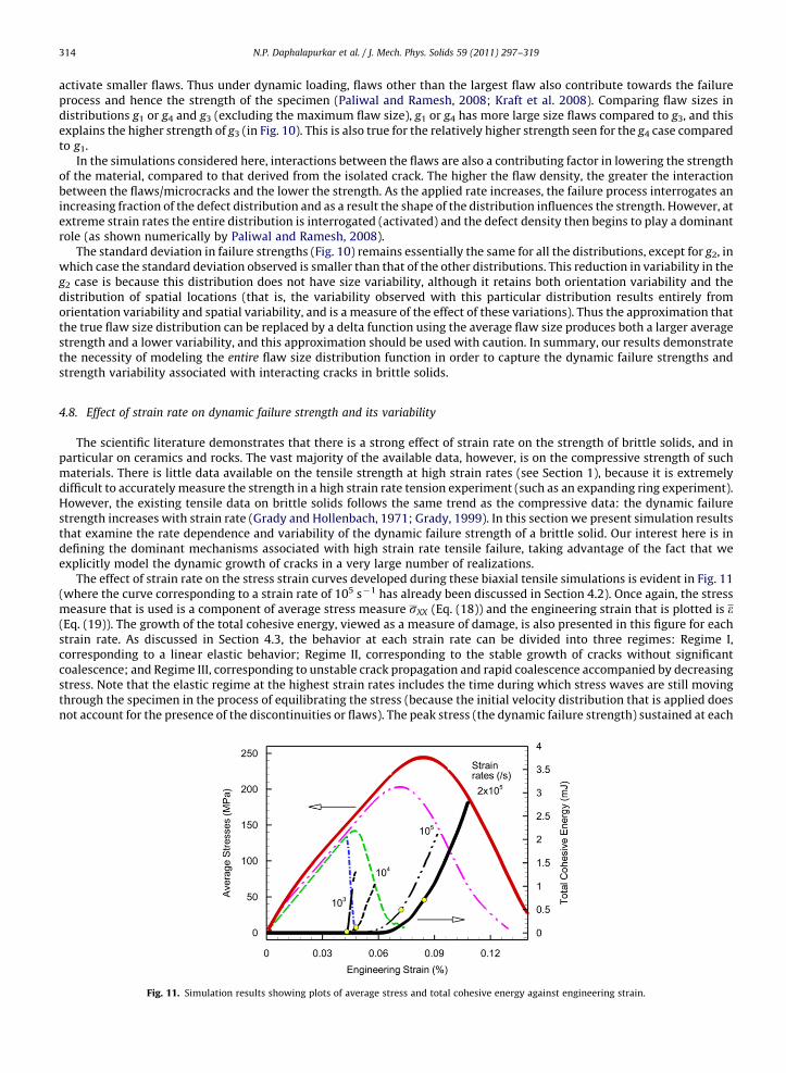
We use the average stress as a characteristic stress measure for the specimens in the discussions that follow, and define themaximum value of the smaller of the two average normal stresses as the ‘‘strength’’ of that realization of the material.The measure of damage that we will use corresponds to the total cohesive energy generated within the specimens during thedeformation (the cohesive energy is summed over all the cohesive elements that have been dynamically inserted withinthe specimen at any given point in the simulation). This is also plotted in Fig. 5 for this specific simulation.
The stress–strain curves that are obtained during the simulations can be divided into three characteristic regimes based onthe fracture processes observed in the microstructure: (I) a linear elastic regime during which no crack growth occurs, (II) anon-linear elastic regime during which stable crack growth occurs, and (III) a collapse regime during which unstable crackgrowth dominates the behavior. The snapshots in Fig. 5A–G show contour plots of the local value of the stress component(sxx) at various points during the deformation, represented by A, B, C, etc. in the overall stress–strain curve. Snapshot(A) shows the microcracked specimen in the undeformed configuration. As the strain is increased the average stress in thespecimen increases with crack-tips acting as stress concentrators (snapshot [B] at a strain of 0.03%). The initial portion of thestrain–strain curve is elastic with no microstructural damage or energy dissipation due to fracture up to a strain ofe=exx=eyy�0.047% (snapshot C). The slope of this portion (between B and C) would be the overall stiffness (equivalentdirectional modulus) of the specimen, which takes into account the microcracked (initially damaged) structure. The averageshear stress (not shown) in the sample is very small compared with the normal stress components. The heterogeneityassociated with the random orientation of the microcracks results in general different stiffness along X (horizontal) and
Fig. 5. Representative simulation results of specimen in biaxial tension showing the resulting stress–strain, damage–strain curves, and microstructural
evolution (A–G) showing microcracked patterns and contours of local stress component sxx. Snapshots indicate specimen in (A) initial configuration,
(B) within elastic regime with no damage, (C) a microcrack is activated and damage initiates, (D) at peak stress, (E) at the peak value for rate of damage growth
and softening on the stress–strain curve, (F) within a regime corresponding to decreasing rate of damage, and (G) corresponding to complete failure and zero
stress (sXX) on the stress–strain curve.
N.P. Daphalapurkar et al. / J. Mech. Phys. Solids 59 (2011) 297–319308
Y (vertical) axes for any given realization. In this particular initial microcracked structure, there are a number of larger cracksoriented preferably along the Y-axis, thus leading to a relatively stiffer response along the Y-axis, as is apparent by comparingthe slopes in the stress–strain plots for sxx and syy.
The beginning of damage (fracture energy dissipation) is associated with the beginning of the second regime (Regime II)during which stable crack-tip propagation occurs, and this typically corresponds to a non-linear portion of the stress–straincurve until a peak stress is reached, between C and D. The amount of additional stress that the specimen can withstand oncecrack growth begins depends on the dominance of loading rate over the kinetics of crack growth. For this particular strain rateof 105/s this non-linear regime spans over a strain (De�0.024%) indicating that the crack growth rates are relatively highcompared with the loading rate (for these tensile conditions the limiting crack speed is a portion of the Rayleigh wave speed).The cohesive energy dissipated in the growing cracks begins to increase at the start of Regime II as shown in Fig. 5, and at theend of this regime the stress reaches a peak, which is the specimen strength.
N.P. Daphalapurkar et al. / J. Mech. Phys. Solids 59 (2011) 297–319 309
The third regime (Regime III) corresponds to the portion of the stress–strain characterized by decreasing stress for furtherincrease in strain, corresponding to the unstable growth of microcracks in the specimen. Snapshot (D), corresponding to astrain of 0.071%, shows that numerous microcracks are activated (a few of them are indicated using circles). Due to thediscrete orientations assigned to the microcracks, it is evident that the stress-field interactions between cracks are not justdependent on the spacing of cracks, but also on the relative orientations of the neighboring cracks and their sizes. This resultsin the activation of flaw sizes which are even smaller than the largest flaw size (indicated by an arrow) in snapshot (D). Thestress drop occurs over a strain of �0.059%, as opposed to a sharp drop in the stress–strain curve observed in experiments.This serves as an indication that the loading rate (105/s in this case) is in the dynamic regime and strength is dominated by thekinetics of crack growth. For this rate of loading, failure of the specimen is as a result of activation, growth and coalescence of anumber of pre-defined microcracks. These processes are evident in snapshot (E) during which the rate of damage has reacheda peak and continue until a strain of 0.1% indicated by snapshot (F), and divides the specimen into a number of fragments[snapshot (G)]. Some smaller sized microcracks (33% of the total flaws in Fig. 5F remain unactivated and are indicated bydotted circles in snapshot). This is consistent with the dynamic regime of flaw dominated fracture.
4.4. The influence of stochasticity on the failure strength
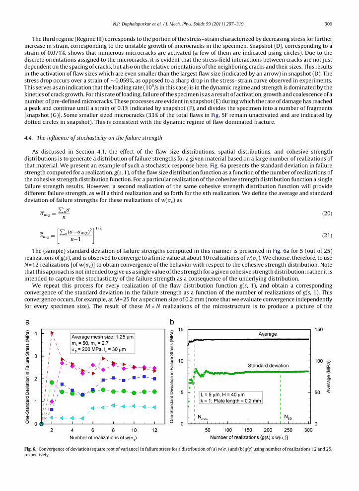
As discussed in Section 4.1, the effect of the flaw size distributions, spatial distributions, and cohesive strengthdistributions is to generate a distribution of failure strengths for a given material based on a large number of realizations ofthat material. We present an example of such a stochastic response here. Fig. 6a presents the standard deviation in failurestrength computed for a realization, g(s, 1), of the flaw size distribution function as a function of the number of realizations ofthe cohesive strength distribution function. For a particular realization of the cohesive strength distribution function a singlefailure strength results. However, a second realization of the same cohesive strength distribution function will providedifferent failure strength, as will a third realization and so forth for the nth realization. We define the average and standarddeviation of failure strengths for these realizations of w(sc) as
savg ¼
Pns
nð20Þ
Savg ¼
Pnðs�savgÞ
2
n�1
" #1=2
ð21Þ
The (sample) standard deviation of failure strengths computed in this manner is presented in Fig. 6a for 5 (out of 25)realizations of g(s), and is observed to converge to a finite value at about 10 realizations of w(sc). We choose, therefore, to useN=12 realizations [of w(sc)] to obtain convergence of the behavior with respect to the cohesive strength distribution. Notethat this approach is not intended to give us a single value of the strength for a given cohesive strength distribution; rather it isintended to capture the stochasticity of the failure strength as a consequence of the underlying distribution.
We repeat this process for every realization of the flaw distribution function g(s, 1), and obtain a correspondingconvergence of the standard deviation in the failure strength as a function of the number of realizations of g(s, 1). Thisconvergence occurs, for example, at M=25 for a specimen size of 0.2 mm (note that we evaluate convergence independentlyfor every specimen size). The result of these M�N realizations of the microstructure is to produce a picture of the
Fig. 6. Convergence of deviation (square root of variance) in failure stress for a distribution of (a) w(sc) and (b) g(s) using number of realizations 12 and 25,
respectively.
N.P. Daphalapurkar et al. / J. Mech. Phys. Solids 59 (2011) 297–319310
stochasticity of the failure strength of the material, and the total number of realizations needed to do this is shown in Fig. 6b tobe on the order of 250–300. Given that we are capturing the dynamic growth of an explicit population of microcracks, this is avery extensive and intensive set of calculations that is needed in order to understand the stochasticity.
Note that the standard deviation in failure strength was of the order of 1.5 MPa when realizations of the cohesive strengthdistribution alone were being considered (Fig. 6a), but the standard deviation of the failure strength is of the order of 8 MPa(Fig. 6b) when the combination of both flaw size distribution and cohesive strength (and their random spatial) distributionare considered. This might be expected, since there is a greater range of variability provided by adding a second distributionfunction, but to obtain a quantitative estimate of this variability requires simulations such as the ones performed here. Fig. 6bshows the number of samples required to obtain an estimated error of 1% (with respect to the value obtained for 300 samples)for average (NAVG) and standard deviation (NSD). It indicates that larger number of samples are required to get convergence inthe standard deviation than the average value.
Traditionally, the variation in failure strengths is considered to be mainly due to variability in the maximum size of defects,and is commonly represented in terms of Weibull-type discussions of size effects (discussed in the next section). However, inthe approach considered here, even though the maximum size of the defect remains the same in all the realizations, avariation in failure strengths is captured as a result of the spatial location of initial microcracks, the interaction between theirstress fields with the neighboring microcracks and the distributions of cohesive strengths associated with subscalemicrostructure. These result in intrinsic stochasticity that couples into the dynamic loading problem through crack growthdynamics, and such behavior is critical for the large-scale computational modeling of brittle materials subjected to dynamicloading (e.g. through incorporation into local variability in material response in the work of Brannon et al., 2007).
4.5. Effect of homogenization of flaw distribution on failure properties
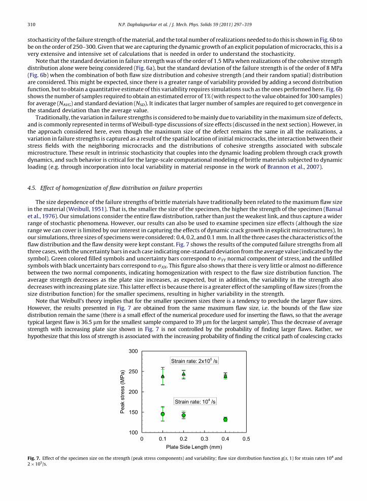
The size dependence of the failure strengths of brittle materials have traditionally been related to the maximum flaw sizein the material (Weibull, 1951). That is, the smaller the size of the specimen, the higher the strength of the specimen (Bansalet al., 1976). Our simulations consider the entire flaw distribution, rather than just the weakest link, and thus capture a widerrange of stochastic phenomena. However, our results can also be used to examine specimen size effects (although the sizerange we can cover is limited by our interest in capturing the effects of dynamic crack growth in explicit microstructures). Inour simulations, three sizes of specimens were considered: 0.4, 0.2, and 0.1 mm. In all the three cases the characteristics of theflaw distribution and the flaw density were kept constant. Fig. 7 shows the results of the computed failure strengths from allthree cases, with the uncertainty bars in each case indicating one-standard deviation from the average value (indicated by thesymbol). Green colored filled symbols and uncertainty bars correspond to sYY normal component of stress, and the unfilledsymbols with black uncertainty bars correspond to sXX. This figure also shows that there is very little or almost no differencebetween the two normal components, indicating homogenization with respect to the flaw size distribution function. Theaverage strength decreases as the plate size increases, as expected, but in addition, the variability in the strength alsodecreases with increasing plate size. This latter effect is because there is a greater effect of the sampling of flaw sizes (from thesize distribution function) for the smaller specimens, resulting in higher variability in the strength.
Note that Weibull’s theory implies that for the smaller specimen sizes there is a tendency to preclude the larger flaw sizes.However, the results presented in Fig. 7 are obtained from the same maximum flaw size, i.e. the bounds of the flaw sizedistribution remain the same (there is a small effect of the numerical procedure used for inserting the flaws, so that the averagetypical largest flaw is 36.5 mm for the smallest sample compared to 39 mm for the largest sample). Thus the decrease of averagestrength with increasing plate size shown in Fig. 7 is not controlled by the probability of finding larger flaws. Rather, wehypothesize that this loss of strength is associated with the increasing probability of finding the critical path of coalescing cracks
Fig. 7. Effect of the specimen size on the strength (peak stress components) and variability; flaw size distribution function g(s, 1) for strain rates 104 and
2�105/s.
N.P. Daphalapurkar et al. / J. Mech. Phys. Solids 59 (2011) 297–319 311
that determines the strength of a given plate (Kraft et al., 2008), since one would expect that the probability of finding such acritical path is higher at any given stress level for a larger plate. In addition to the possibility of achieving a critical path, a loss ofstrength may be associated with the development of critical crack clusters that lead to highly unstable crack growth (and theprobability of developing such a cluster may increase with specimen size). Note that we are examining a large number ofrealizations for every plate as discussed in the previous section, and it is likely that some of those realizations for any given platesize will have arrangements of flaws that provide the critical path at a low stress, resulting (in some exceptional cases) in relativelylow strengths for the smaller plates (as seen in the variability). Similar trends in the size-scaling of failure strengths have beenobserved in the experimental results from ring-on-ring (biaxial tension) tests on AlN reported by Wereszczak et al. (1999). There isvery little systematic study of the variability in the strength of the solids as a function of specimen size, and we would like toencourage the development of such data. Broadly similar observations of decreasing strength with increasing specimen size areabundant in the literature under other stress states, although it is usually claimed that this is due to the probability of finding largeflaws, without paying as much attention to the influence of the shape of the flaw size distribution function. We show in Section 4.7that the shape of the flaw size distribution function can play a significant role in size scaling and strength variability.
4.6. Implications for the variation of strength in large-scale simulations
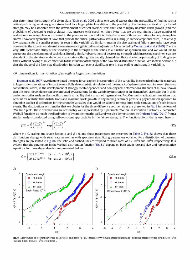
Brannon et al., 2007 have demonstrated the need for an explicit incorporation of the variability in strength of ceramic materialsin large-scale simulations of impact events. Fully deterministic simulations of the impact of spheres into ceramics result (in mostconventional codes) in the development of strongly mesh-dependent and non-physical deformations. Brannon et al. have shownthat the mesh-dependence can be eliminated by accounting for the variability in strength at an element/cell size scale, but in theirand other similar analyses the specific strength variability that is assumed is generally ad hoc. Our multi-realization simulations thataccount for realistic flaw distributions and dynamic crack growth in engineering ceramics provide a physics-based approach toobtaining explicit distributions for the strengths at scales that would be subgrid to most large-scale simulations of such impactevents. The distributions of strengths that we obtain for the three different specimen sizes are presented in Fig. 8 in the form of‘‘Weibull’’ plots. These distributions are reasonably well represented by 3-parameter Weibull distribution functions. 2-parameterWeibull functions do not fit the distribution of dynamic strengths well, and was also demonstrated by Graham-Brady (2010) from asimilar analysis conducted using self-consistent approach for brittle failure strengths. The functional form that is used here is
f ðsÞ ¼ ba
s�C
a
� �b�1
exps�C
a
� �b" #
ð22Þ
where s4C, scaling and shape factors a and b40, and these parameters are presented in Table 2. Fig. 8a shows that thesedistributions change with strain rate as well as with specimen size. Fitting parameters obtained for a distribution of dynamicstrengths are presented in Fig. 8b; the solid and dashed lines correspond to strain rates of 2�105/s and 104/s, respectively. It isevident that the parameters in the Weibull distribution function (Fig. 8b) depend on both strain rate and size, and representativeequations for these dependencies are presented below:
C ¼132:7L0:0429 for _e ¼ 1� 104=s
251:74L0:055 for _e ¼ 2� 105=s
( )ð23aÞ
Fig. 8. Distribution of strength (average peak stress) and fits for a (a) 3-parameter Weibull distribution fits and (b) fitting parameters for strain rates 104/s
(dashed lines) and 2�105/s (solid lines).
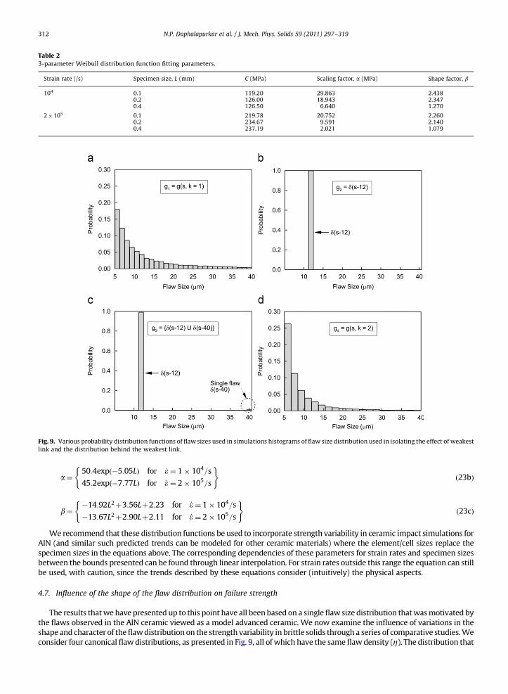
Table 23-parameter Weibull distribution function fitting parameters.
Strain rate (/s) Specimen size, L (mm) C (MPa) Scaling factor, a (MPa) Shape factor, b
104 0.1 119.20 29.863 2.4380.2 126.00 18.943 2.3470.4 126.50 6.640 1.270
2�105 0.1 219.78 20.752 2.2600.2 234.67 9.591 2.1400.4 237.19 2.021 1.079
Fig. 9. Various probability distribution functions of flaw sizes used in simulations histograms of flaw size distribution used in isolating the effect of weakest
link and the distribution behind the weakest link.
N.P. Daphalapurkar et al. / J. Mech. Phys. Solids 59 (2011) 297–319312
a¼50:4expð�5:05LÞ for _e ¼ 1� 104=s
45:2expð�7:77LÞ for _e ¼ 2� 105=s
( )ð23bÞ
b¼�14:92L2þ3:56Lþ2:23 for _e ¼ 1� 104=s
�13:67L2þ2:90Lþ2:11 for _e ¼ 2� 105=s
( )ð23cÞ
We recommend that these distribution functions be used to incorporate strength variability in ceramic impact simulations forAlN (and similar such predicted trends can be modeled for other ceramic materials) where the element/cell sizes replace thespecimen sizes in the equations above. The corresponding dependencies of these parameters for strain rates and specimen sizesbetween the bounds presented can be found through linear interpolation. For strain rates outside this range the equation can stillbe used, with caution, since the trends described by these equations consider (intuitively) the physical aspects.
4.7. Influence of the shape of the flaw distribution on failure strength
The results that we have presented up to this point have all been based on a single flaw size distribution that was motivated bythe flaws observed in the AlN ceramic viewed as a model advanced ceramic. We now examine the influence of variations in theshape and character of the flaw distribution on the strength variability in brittle solids through a series of comparative studies. Weconsider four canonical flaw distributions, as presented in Fig. 9, all of which have the same flaw density (Z). The distribution that
N.P. Daphalapurkar et al. / J. Mech. Phys. Solids 59 (2011) 297–319 313
we have considered up to this point is presented in Fig. 9a and will be referred to as distribution g1. Fig. 9b presents a flawdistribution (g2) that is equivalent to that in Fig. 9a in that it has the same average flaw size, but the distribution is a delta function(that is, all of the flaws have the same size as the average flaw size in g1). Note that this implies that all of the flaws in the ceramichave the same size, but they still have uniform distributions of orientation and spatial location. A comparison of the effects ofdistributions g1 and g2 allows us to focus on the influence of distributions of size. We next introduce a third flaw size distributiong3, which is identical to g2 except that it contains a single large flaw at the upper bound of the size distribution in g1. A comparisonof the effects of flaw distributions g2 and g3 allows us to focus on the influence of the weakest link (that is the largest flaw) on thebehavior of the ceramic. Finally, we consider a Pareto distribution similar to that in g1 except that the shape parameter k is set to 2(Fig. 9d), so that a comparison of the effects of distributions g4 and g1 provides an understanding of the influence of the shape of theflaw distribution (we note that companies that make engineering ceramics must determine what shapes of the flaw sizedistribution function to target for their ceramic products). The primary difference between g4 and g1 is that the ceramic containingg4 has many more small flaws and fewer large flaws.
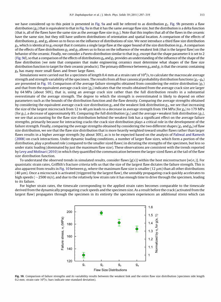
Simulations were carried out for a specimen of length 0.4 mm at a strain rate of 104/s, to calculate the macroscale averagestrength and strength variability of the specimen. The results from all four canonical probability distribution functions (g1–g4)are presented in Fig. 10. Comparison of the average failure strengths obtained from considering the entire distribution (g1)and that from the equivalent average crack size (g2) indicates that the results obtained from the average crack size are largerby 64 MPa (about 50%), that is, using an average crack size rather than the full distribution results in a substantialoverestimate of the average strength. The degree to which the strength is overestimated is likely to depend on otherparameters such as the bounds of the distribution function and the flaw density. Comparing the average strengths obtainedby considering the equivalent average crack size distribution g2 and the weakest link distribution g3, we see that increasingthe size of the largest microcrack from 12 to 40 mm leads to a decrease in average strength from 194 MPa (for g2) to 179 MPa(for g3), a decrease of approximately 8%. Comparing the full distribution (g1) and the average+weakest link distribution (g3),we see that accounting for the flaw size distribution behind the weakest link has a significant effect on the average failurestrengths, primarily because for interacting cracks the crack size distribution plays a critical role in the development of thefailure strength. Finally, comparing the average strengths obtained by considering the two different shapes (g1 and g4) of flawsize distribution, we see that the flaw size distribution that is more heavily weighted toward smaller flaws rather than largerflaws results in a higher average strength (by about 30%), as is to be expected based on the analysis of Paliwal and Ramesh(2008) on crack interactions. Under dynamic loading conditions, a number of larger flaw sizes, which form a portion of thedistribution, play a profound role (compared to the smaller sized flaws) in dictating the strengths of the specimen, but less sounder static loading (dominated by just the maximum flaw size). These observations are consistent with the trends reportedby Levy and Molinari (2010) in which they quantified the communication between the larger sized flaws at the tail of the flawsize distribution function.
To understand the observed trends in simulated results, consider flaws [g(s)] within the host microstructure [w(sc)]. Forquasistatic strain rates, Griffith’s fracture criteria tells us that the size of the largest flaw dictates the failure strength. This isalso apparent from results in Fig. 10 between g2 where the maximum flaw size is smaller (12 mm) than all other distributions(40 mm). Once a microcrack is activated (triggered by the largest flaw), the unstably propagating crack quickly accelerates tohigh speeds (�2500 m/s), and due to the relatively low strain rate it has enough time to drive through the specimen, leadingto its failure.
For higher strain rates, the timescale corresponding to the applied strain rates becomes comparable to the timescalederived from the dynamically propagating crack speeds and the specimen size. As a result before the crack (activated from thelargest flaw) propagates through the specimen in its entirety the specimen experiences an additional stress which can
Fig. 10. Comparison of failure strengths and its variability results between the weakest link and the entire flaw size distribution (specimen side length
0.2 mm; strain-rate 104/s; bars indicate one-standard deviation).
N.P. Daphalapurkar et al. / J. Mech. Phys. Solids 59 (2011) 297–319314
activate smaller flaws. Thus under dynamic loading, flaws other than the largest flaw also contribute towards the failureprocess and hence the strength of the specimen (Paliwal and Ramesh, 2008; Kraft et al. 2008). Comparing flaw sizes indistributions g1 or g4 and g3 (excluding the maximum flaw size), g1 or g4 has more large size flaws compared to g3, and thisexplains the higher strength of g3 (in Fig. 10). This is also true for the relatively higher strength seen for the g4 case comparedto g1.
In the simulations considered here, interactions between the flaws are also a contributing factor in lowering the strengthof the material, compared to that derived from the isolated crack. The higher the flaw density, the greater the interactionbetween the flaws/microcracks and the lower the strength. As the applied rate increases, the failure process interrogates anincreasing fraction of the defect distribution and as a result the shape of the distribution influences the strength. However, atextreme strain rates the entire distribution is interrogated (activated) and the defect density then begins to play a dominantrole (as shown numerically by Paliwal and Ramesh, 2008).
The standard deviation in failure strengths (Fig. 10) remains essentially the same for all the distributions, except for g2, inwhich case the standard deviation observed is smaller than that of the other distributions. This reduction in variability in theg2 case is because this distribution does not have size variability, although it retains both orientation variability and thedistribution of spatial locations (that is, the variability observed with this particular distribution results entirely fromorientation variability and spatial variability, and is a measure of the effect of these variations). Thus the approximation thatthe true flaw size distribution can be replaced by a delta function using the average flaw size produces both a larger averagestrength and a lower variability, and this approximation should be used with caution. In summary, our results demonstratethe necessity of modeling the entire flaw size distribution function in order to capture the dynamic failure strengths andstrength variability associated with interacting cracks in brittle solids.
4.8. Effect of strain rate on dynamic failure strength and its variability
The scientific literature demonstrates that there is a strong effect of strain rate on the strength of brittle solids, and inparticular on ceramics and rocks. The vast majority of the available data, however, is on the compressive strength of suchmaterials. There is little data available on the tensile strength at high strain rates (see Section 1), because it is extremelydifficult to accurately measure the strength in a high strain rate tension experiment (such as an expanding ring experiment).However, the existing tensile data on brittle solids follows the same trend as the compressive data: the dynamic failurestrength increases with strain rate (Grady and Hollenbach, 1971; Grady, 1999). In this section we present simulation resultsthat examine the rate dependence and variability of the dynamic failure strength of a brittle solid. Our interest here is indefining the dominant mechanisms associated with high strain rate tensile failure, taking advantage of the fact that weexplicitly model the dynamic growth of cracks in a very large number of realizations.
The effect of strain rate on the stress strain curves developed during these biaxial tensile simulations is evident in Fig. 11(where the curve corresponding to a strain rate of 105 s�1 has already been discussed in Section 4.2). Once again, the stressmeasure that is used is a component of average stress measure sXX (Eq. (18)) and the engineering strain that is plotted is e(Eq. (19)). The growth of the total cohesive energy, viewed as a measure of damage, is also presented in this figure for eachstrain rate. As discussed in Section 4.3, the behavior at each strain rate can be divided into three regimes: Regime I,corresponding to a linear elastic behavior; Regime II, corresponding to the stable growth of cracks without significantcoalescence; and Regime III, corresponding to unstable crack propagation and rapid coalescence accompanied by decreasingstress. Note that the elastic regime at the highest strain rates includes the time during which stress waves are still movingthrough the specimen in the process of equilibrating the stress (because the initial velocity distribution that is applied doesnot account for the presence of the discontinuities or flaws). The peak stress (the dynamic failure strength) sustained at each
Fig. 11. Simulation results showing plots of average stress and total cohesive energy against engineering strain.
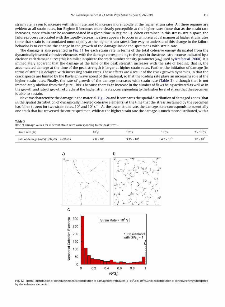
N.P. Daphalapurkar et al. / J. Mech. Phys. Solids 59 (2011) 297–319 315
strain rate is seen to increase with strain rate, and to increase more rapidly at the higher strain rates. All three regimes areevident at all strain rates, but Regime II becomes more clearly perceptible at the higher rates (note that as the strain rateincreases, more strain can be accommodated in a given time in Regime II). When examined in this stress–strain space, thefailure process associated with the rapidly decreasing stress appears to occur in a more gradual manner at higher strain rates(note that strain is accumulated more rapidly at the higher strain rates). One way to understand this change in the failurebehavior is to examine the change in the growth of the damage inside the specimens with strain rate.
The damage is also presented in Fig. 11 for each strain rate in terms of the total cohesive energy dissipated from thedynamically inserted cohesive elements, with the damage corresponding to the peak in the stress–strain curve indicated by acircle on each damage curve (this is similar in spirit to the crack number density parameter (oN) used by Kraft et al., 2008). It isimmediately apparent that the damage at the time of the peak strength increases with the rate of loading, that is, theaccumulated damage at the time of the peak strength is larger at higher strain rates. Further, the initiation of damage (interms of strain) is delayed with increasing strain rates. These effects are a result of the crack growth dynamics, in that thecrack speeds are limited by the Rayleigh wave speed of the material, so that the loading rate plays an increasing role at thehigher strain rates. Finally, the rate of growth of the damage increases with strain rate (Table 3), although that is notimmediately obvious from the figure. This is because there is an increase in the number of flaws being activated as well as inthe growth and rate of growth of cracks at the higher strain rates, corresponding to the higher level of stress that the specimenis able to sustain.
Next, we characterize the damage in the material. Fig. 12a and b compares the spatial distribution of damaged zones (thatis, the spatial distribution of dynamically inserted cohesive elements) at the time that the stress sustained by the specimenhas fallen to zero for two strain rates, 103 and 105 s�1. At the lower strain rate, the damage state corresponds to essentiallyone crack that has traversed the entire specimen, while at the higher strain rate the damage is much more distributed, with a
Table 3Rate of damage values for different strain rates corresponding to the peak stress.
Strain rate (/s) 103/s 104/s 105/s 2�105/s
Rate of damage (mJ/s): ð@O=@tÞ ¼ _eð@O=@eÞ 2.8�104 3.35�104 4.7�105 12�105
Fig. 12. Spatial-distribution of cohesive elements contribution to damage for strain rates (a) 103, (b) 105/s, and (c) distribution of cohesive energy dissipated
by the cohesive elements.
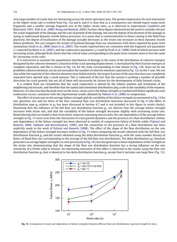
N.P. Daphalapurkar et al. / J. Mech. Phys. Solids 59 (2011) 297–319316
very large number of cracks that are interacting across the entire specimen area. The greater importance of crack interactionat the higher strain rate is evident from Fig. 12a and b, and it is clear that as a consequence one should expect many morefragments and a smaller average fragment size at the higher strain rates, as is observed in experiments (Lankford andBlanchard, 1991; Shih et al., 2000; Wang and Ramesh, 2004). Further, these figures demonstrate the need to consider not justthe scalar magnitude of the damage and the rate of growth of the damage, but also the degree of localization of the damage intrying to understand dynamic tensile failure processes. In a sense that is counterintuitive to those coming to the field fromplasticity, the degree of localization of the damage actually decreases as the strain rate increases in these dynamic tensilefailure problems. We can compare the results of localized damage from our simulations with those reported by grain-levelsimulations (Kraft et al., 2008; Maiti et al., 2005). The results reported here are consistent with the fragment size parameter(l) reported by Maiti et al. (2005), and the coalescence parameter (w) used by Kraft et al. (2008), both of which increase withincreasing strain, although Kraft shows that the critical value corresponding to the peak stress remains more or less the samefor increasing strain rates.
It is instructive to examine the quantitative distribution of damage in the sense of the distribution of cohesive energiesdissipated by the cohesive elements (a function of the crack opening displacement, d) normalized by their fracture energies atcomplete separation, and this is shown in Fig. 12c for the state corresponding to that shown in Fig. 12b. Since we do notpredefine cohesive elements, we do not normalize the number of cohesive elements reported in Fig. 12c on the Y-axis. We seethat while the majority of the cohesive elements have failed entirely, the largest fraction of the ones that have not completelyseparated have opened only a small amount. This is indicated of the fact that the system is probing a number of possibledirections for crack growth, but not all of them will necessarily be chosen for the development of fully formed cracks.
It is evident from our simulations that the crack coalescence is altered by the relative position and orientation of theneighboring microcracks, and therefore that the spatial and orientation distributions play a role in the variability of the response.However, it is also true that the peak stress on the stress–strain curve (the failure strength) is reached well before significant crackcoalescence occurs, consistent with the experimental results obtained by Paliwal et al. (2006) in compression.
The effect of strain rate on the average failure strength and the variability of the failure strength are presented in Fig. 13 forone specimen size and for three of the four canonical flaw size distribution functions discussed in Fig. 9 (the effect ofdistribution type g4 relative to g3 has been discussed in Section 4.7 and is not included in this figure to retain clarity).Examining first the influence of the full flaw size distribution function g1, we observe that the average failure strengthincreases with strain rate, and that the variability of the failure strength decreases slightly with increasing strain rate.Remembering that our model is that of an elastic material containing microcracks, the rate dependence of the average failurestrength in Fig. 13 must arise from the interaction of crack growth dynamics and the presence of a flaw distribution. Similarrate dependence of the failure strength has been observed in models of compressive failure of brittle solids (Paliwal andRamesh, 2008; Subhash and Ravichandran, 1998), and the connection to the presence of a flaw distribution has beenexplicitly made in the work of Paliwal and Ramesh (2008). The effect of the shape of the flaw distribution on the ratedependence of the failure strength becomes evident in Fig. 13 when comparing the results obtained with the full flaw sizedistribution function g1 and the results obtained using the delta distribution function g2 with the same number density offlaws (of fixed flaw size corresponding to the average of the full flaw size distribution). The delta distribution (g2) functiongenerates on average higher strengths (as seen previously in Fig. 10), but also generates a lower dependence of the strength onthe strain rate, demonstrating that the shape of the flaw size distribution function has a strong influence on the ratesensitivity of a brittle solid in tension. An interesting extension of this effect is observed in the results using the flaw sizedistribution function g3 that is identical to the delta distribution function g2 except that it includes one large flaw (Fig. 13).
Fig. 13. Comparison of strain-rate dependence of failure strengths between different flaw size distributions (specimen length 0.2 mm).
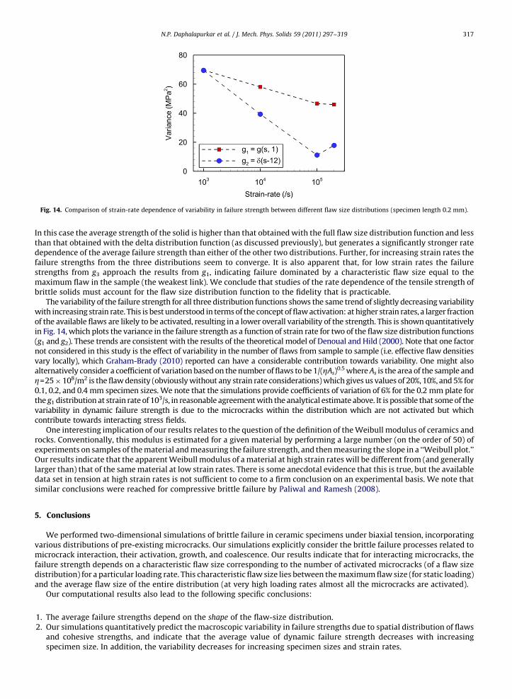
Fig. 14. Comparison of strain-rate dependence of variability in failure strength between different flaw size distributions (specimen length 0.2 mm).
N.P. Daphalapurkar et al. / J. Mech. Phys. Solids 59 (2011) 297–319 317
In this case the average strength of the solid is higher than that obtained with the full flaw size distribution function and lessthan that obtained with the delta distribution function (as discussed previously), but generates a significantly stronger ratedependence of the average failure strength than either of the other two distributions. Further, for increasing strain rates thefailure strengths from the three distributions seem to converge. It is also apparent that, for low strain rates the failurestrengths from g3 approach the results from g1, indicating failure dominated by a characteristic flaw size equal to themaximum flaw in the sample (the weakest link). We conclude that studies of the rate dependence of the tensile strength ofbrittle solids must account for the flaw size distribution function to the fidelity that is practicable.
The variability of the failure strength for all three distribution functions shows the same trend of slightly decreasing variabilitywith increasing strain rate. This is best understood in terms of the concept of flaw activation: at higher strain rates, a larger fractionof the available flaws are likely to be activated, resulting in a lower overall variability of the strength. This is shown quantitativelyin Fig. 14, which plots the variance in the failure strength as a function of strain rate for two of the flaw size distribution functions(g1 and g2). These trends are consistent with the results of the theoretical model of Denoual and Hild (2000). Note that one factornot considered in this study is the effect of variability in the number of flaws from sample to sample (i.e. effective flaw densitiesvary locally), which Graham-Brady (2010) reported can have a considerable contribution towards variability. One might alsoalternatively consider a coefficient of variation based on the number of flaws to be 1/(ZAs)
0.5 where As is the area of the sample andZ=25�108/m2 is the flaw density (obviously without any strain rate considerations) which gives us values of 20%, 10%, and 5% for0.1, 0.2, and 0.4 mm specimen sizes. We note that the simulations provide coefficients of variation of 6% for the 0.2 mm plate forthe g1 distribution at strain rate of 103/s, in reasonable agreement with the analytical estimate above. It is possible that some of thevariability in dynamic failure strength is due to the microcracks within the distribution which are not activated but whichcontribute towards interacting stress fields.
One interesting implication of our results relates to the question of the definition of the Weibull modulus of ceramics androcks. Conventionally, this modulus is estimated for a given material by performing a large number (on the order of 50) ofexperiments on samples of the material and measuring the failure strength, and then measuring the slope in a ‘‘Weibull plot.’’Our results indicate that the apparent Weibull modulus of a material at high strain rates will be different from (and generallylarger than) that of the same material at low strain rates. There is some anecdotal evidence that this is true, but the availabledata set in tension at high strain rates is not sufficient to come to a firm conclusion on an experimental basis. We note thatsimilar conclusions were reached for compressive brittle failure by Paliwal and Ramesh (2008).
5. Conclusions
We performed two-dimensional simulations of brittle failure in ceramic specimens under biaxial tension, incorporatingvarious distributions of pre-existing microcracks. Our simulations explicitly consider the brittle failure processes related tomicrocrack interaction, their activation, growth, and coalescence. Our results indicate that for interacting microcracks, thefailure strength depends on a characteristic flaw size corresponding to the number of activated microcracks (of a flaw sizedistribution) for a particular loading rate. This characteristic flaw size lies between the maximum flaw size (for static loading)and the average flaw size of the entire distribution (at very high loading rates almost all the microcracks are activated).
Our computational results also lead to the following specific conclusions:
1.
The average failure strengths depend on the shape of the flaw-size distribution. 2. Our simulations quantitatively predict the macroscopic variability in failure strengths due to spatial distribution of flawsand cohesive strengths, and indicate that the average value of dynamic failure strength decreases with increasingspecimen size. In addition, the variability decreases for increasing specimen sizes and strain rates.
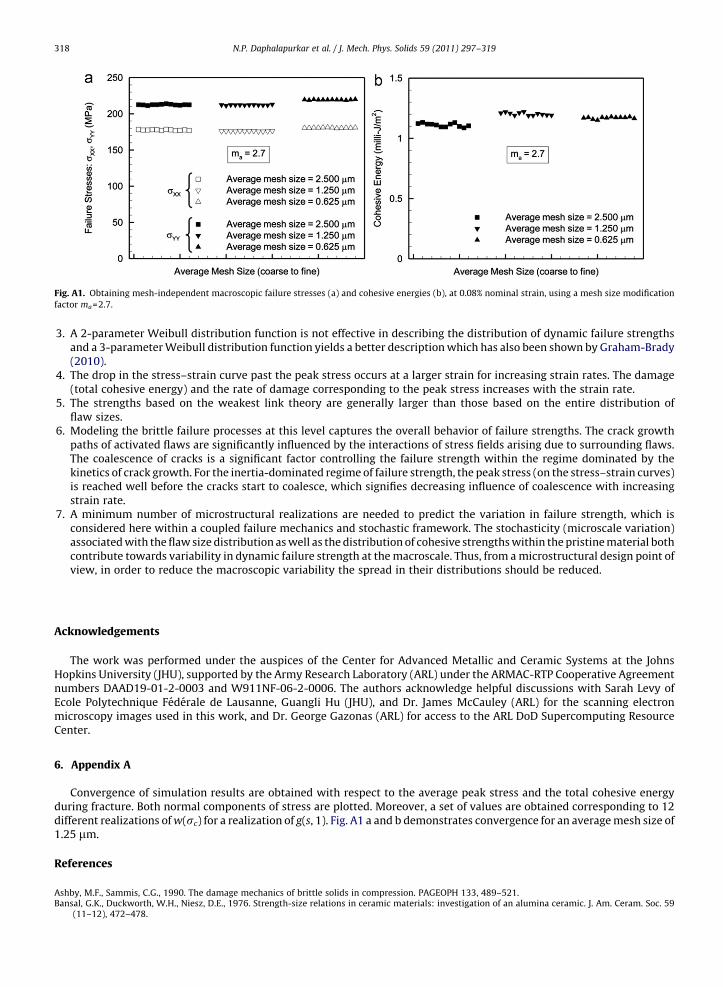
Fig. A1. Obtaining mesh-independent macroscopic failure stresses (a) and cohesive energies (b), at 0.08% nominal strain, using a mesh size modification
factor ma=2.7.
N.P. Daphalapurkar et al. / J. Mech. Phys. Solids 59 (2011) 297–319318
3.
A 2-parameter Weibull distribution function is not effective in describing the distribution of dynamic failure strengthsand a 3-parameter Weibull distribution function yields a better description which has also been shown by Graham-Brady(2010).4.
The drop in the stress–strain curve past the peak stress occurs at a larger strain for increasing strain rates. The damage(total cohesive energy) and the rate of damage corresponding to the peak stress increases with the strain rate.5.
The strengths based on the weakest link theory are generally larger than those based on the entire distribution offlaw sizes.6.
Modeling the brittle failure processes at this level captures the overall behavior of failure strengths. The crack growthpaths of activated flaws are significantly influenced by the interactions of stress fields arising due to surrounding flaws.The coalescence of cracks is a significant factor controlling the failure strength within the regime dominated by thekinetics of crack growth. For the inertia-dominated regime of failure strength, the peak stress (on the stress–strain curves)is reached well before the cracks start to coalesce, which signifies decreasing influence of coalescence with increasingstrain rate.7.
A minimum number of microstructural realizations are needed to predict the variation in failure strength, which isconsidered here within a coupled failure mechanics and stochastic framework. The stochasticity (microscale variation)associated with the flaw size distribution as well as the distribution of cohesive strengths within the pristine material bothcontribute towards variability in dynamic failure strength at the macroscale. Thus, from a microstructural design point ofview, in order to reduce the macroscopic variability the spread in their distributions should be reduced.Acknowledgements
The work was performed under the auspices of the Center for Advanced Metallic and Ceramic Systems at the JohnsHopkins University (JHU), supported by the Army Research Laboratory (ARL) under the ARMAC-RTP Cooperative Agreementnumbers DAAD19-01-2-0003 and W911NF-06-2-0006. The authors acknowledge helpful discussions with Sarah Levy ofEcole Polytechnique Federale de Lausanne, Guangli Hu (JHU), and Dr. James McCauley (ARL) for the scanning electronmicroscopy images used in this work, and Dr. George Gazonas (ARL) for access to the ARL DoD Supercomputing ResourceCenter.
6. Appendix A
Convergence of simulation results are obtained with respect to the average peak stress and the total cohesive energyduring fracture. Both normal components of stress are plotted. Moreover, a set of values are obtained corresponding to 12different realizations of w(sc) for a realization of g(s, 1). Fig. A1 a and b demonstrates convergence for an average mesh size of1.25 mm.
References
Ashby, M.F., Sammis, C.G., 1990. The damage mechanics of brittle solids in compression. PAGEOPH 133, 489–521.Bansal, G.K., Duckworth, W.H., Niesz, D.E., 1976. Strength-size relations in ceramic materials: investigation of an alumina ceramic. J. Am. Ceram. Soc. 59
(11–12), 472–478.
N.P. Daphalapurkar et al. / J. Mech. Phys. Solids 59 (2011) 297–319 319
Belytschko, T., 1983. An overview of semi-discretization and time integration procedures. In: Belytschko, T., Hughes, T.L.J. (Eds.), Computational Methods forTransient Analysis. North-Holland, pp. 1–65.
Brannon, R.M., Wells, J.M., Eric Strack, O., 2007. Validating theories of brittle damage. Metall. Mater. Trans. A 38A, 2861–2868.Broberg, K.B., 1999. Cracks and Fracture. Academic Press.Camacho, G.T., Ortiz, M., 1996. Computational modelling of impact damage in brittle materials. Int. J. Solids Struct. 33 (20–22), 2899–2938.Chen, W.N., Ravichandran, G., 1996. Static and dynamic compressive behavior of aluminum nitride under moderate confinement. J. Am. Ceram. Soc. 79 (3),
579–584.Denoual, C., Hild, F., 2000. A damage model for the dynamic fragmentation of brittle solids. Comput. Methods Appl. Mech. Eng. 183, 247–258.Espinosa, H.D., Zavattieri, P.D., Dwivedi, S., 1998. A finite deformation continuum discrete model for the description of fragmentation and damage in brittle
materials. J. Mech. Phys. Solids 46, 1909–1942.Falk, M.L., Needleman, A., Rice, J.R., 2001. A critical evaluation of cohesive zone models of dynamic fracture. J. Phys. IV Proc., Pr.5.43–Pr.5.50.Grady, D.E., Kipp, M.E., 1980. Continuum modeling of explosive fracture in oil shale. Int. J. Rock. Mech. Min. Sci. Geomech. 17, 147–157.Grady, D.E., 1982. Local inertial effects in dynamic fragmentation. J. Appl. Phys. 53 (1), 322–325.Grady, D.E., Benson, D.A., 1983. Fragmentation of metal rings by electromagnetic loading. Expt. Mech. 23, 393–400.Grady, D.E., Hollenbach, R.E., 1971. Dynamic fracture strength of rock. Geophys. Res. Lett. 6 (2), 73–76.Grady, D.E., 1999. Impact failure and fragmentation properties of tungsten carbide. Int. J. Impact Eng. 23, 307–317.Graham-Brady, L., 2010. Statistical characterization of meso-scale uniaxial compressive strength in brittle materials with randomly occurring flaws. Int. J.
Solids Struct. 47, 2398–2413.Gurvich, M.R., DiBenedetto, A.T., Ranade, S.V., 1997. A new statistical distribution for characterizing the random strength of brittle materials. J. Mater. Sci. 32,
2559–2564.Gutans, J., Tamuzs, V., 1984. Scale effect of the Weibull distribution of fiber strengths. Mech. Comp. Mater. 20, 1107–1109.Huang, C., Subhash, G., 2003. Influence of lateral confinement on dynamic damage evolution during uniaxial compressive response of brittle solids. J. Mech.
Phys. Solids 51, 1089–1106.Hughes, T.L.J., 1987. The Finite Element Method: Linear Static and Dynamic Finite Element Analysis. Prentice-Hall, Englewood Cliffs, NJ.Jayatilaka, A.D.S., Trustrum, K., 1977. Statistical approach to brittle fracture. J. Mater. Sci. 12, 1426–1430.Kraft, R.H., Molinari, J.F., Ramesh, K.T., Warner, D.H., 2008. Computational micromechanics of dynamic compressive loading of a brittle polycrystalline
material using a distribution of grain boundary properties. J. Mech. Phys. Solids 56, 2618–2641.Lamon, J., 1988. Statistical approaches to failure for ceramic reliability assessment. J. Am. Ceram. Soc. 71 (2), 106–112.Lankford, J., 1981. Mechanisms responsible for strain rate dependent compressive strength in ceramic materials. J. Am. Ceram. Soc. 64, C33–C35.Lankford, J., Blanchard, C.R., 1991. Fragmentation of brittle materials at high rates of loading. J. Mater. Sci. 26, 3067–3072.Levy, S., Molinari, J.-F., 2010. Dynamic fragmentation of ceramics, signature of flaws and scaling of fragment sizes. J. Mech. Phys. Solids 58, 12–26.Lindborg, U., 1969. A statistical model for the linking of microcracks. Acta Metall. 17, 521–526.Maiti, S., Rangaswamy, K., Geubelle, P.H., 2005. Mesoscale analysis of dynamic fragmentation of ceramics under tension. Acta Mater. 53, 823–834.Miller, O., Freund, L.B., Needleman, A., 1999. Modeling and simulation of dynamic fragmentation in brittle materials. Int. J. Fract. 96, 101–125.Molinari, J.F., Gazonas, G., Raghupathy, R., Rusinek, A., Zhou, F., 2007. The cohesive element approach to dynamic fragmentation: the question of energy
convergence. Int. J. Numer. Meth. Eng. 69, 484–503.Mott, N.F., 1947. Fragmentation of shell cases. Proc. R. Soc. London A 189, 300–308.Nemat-Nasser, S., Deng, H., 1994. Strain-rate effect on brittle failure in compression. Acta Metall. Mater. 42 (3), 1013–1024.Paliwal, B., Ramesh, K.T., McCauley, J.W., 2006. Direct observation of the dynamic compressive failure of a transparent polycrystalline ceramic (AlON). J. Am.
Ceram. Soc. 89, 2128–2133.Paliwal, B., Ramesh, K.T., 2008. An interacting microcrack damage model for failure of brittle materials under compression. J. Mech. Phys. Solids 56, 896–923.Palmer, A.C., Rice, J.R., 1973. The growth of slip surfaces in the progressive failure of over-consolidated clay. Philos. Trans. R. Soc. London Ser. A 332, 527–548.Pandolfi, A., Krysl, P., Ortiz, M., 1999. Finite element simulation of ring expansion and fragmentation: the capturing of length and time scales through
cohesive models of fracture. Int. J. Fract. 95, 279–297.Pandolfi, A., Ortiz, M., 2002. An efficient adaptive procedure for three-dimensional fragmentation simulations. Eng. Comput. 18, 148–159.Sarva, S., Nemat-Nasser, S., 2001. Dynamic compressive strength of silicon carbide under uniaxial compression. Mater. Sci. Eng. A317, 140–144.Shih, C.J., Meyers, M.A., Nesterenko, V.F., Chen, S.J., 2000. Damage evolution in dynamic deformation of silicon carbide. Acta Mater. 48, 2399–2420.Shockey, D.A., Curran, D.R., Seaman, L., Rosenberg, J.T., Peterson, C.F., 1974. Fragmentation of rocks under dynamic loads. Int. J. Rock Mech. Min. Sci. 11,
303–317.Srolovitz, D.J., Beale, P.D., 1988. Computer simulation of failure in an elastic model with randomly distributed flaws. J. Am. Ceram. Soc. 71 (5), 362–369.Subhash, G., Ravichandran, G., 1998. Mechanical behavior of a hot pressed aluminum nitride under uniaxial compression. J. Mater. Sci. 33, 1933–1939.Trustrum, K., Jayatilaka, A.De.S., 1983. Applicability of Weibull analysis for brittle materials. J. Mater. Sci. 18, 2765–2770.Walter, M.E., Owen, D.W., Ravichandran, G., 1994. Static and dynamic tension testing of ceramics and ceramic composites. Mechanical Testing of Ceramics
and Composites, AMD-Vol. 197.Wang, H., Ramesh, K.T., 2004. Dynamic strength and fragmentation of hot-pressed silicon carbide under uniaxial compression. Acta Mater. 52, 335–367.Watson, A.S., Smith, R.L., 1985. An examination of statistical theories for fibrous materials in the light of experimental data. J. Mater. Sci. 20, 3260–3270.Weibull, W., 1939. A statistical theory of the strength of materials. Proc. R. Swedish Inst. Eng. Res. 151.Weibull, W., 1951. A statistical distribution function of wide applicability. J. Appl. Mech. 18, 292–297.Wereszczak, A.A., Kirkland, T.P., Breder, K., Lin, H.-T., Andrews, A.J., 1999. Biaxial strength, strength-size-scaling, and fatigue resistance of alumina and
aluminum nitride substrates. Int. J. Microcircuits Electron. Packaging 22 (4), 446–458.Zavattieri, P.D., Espinosa, H.D., 2001. Grain level analysis of crack initiation and propagation in brittle materials. Acta Mater. 49 (20), 4291–4311.Zhou, F., Molinari, J.F., 2004. Stochastic fracture of ceramics under dynamic tensile loading. Int. J. Solids Struct. 41, 6573–6596.Zhou, F., Molinari, J.F., 2005. On the rate-dependency of dynamic tensile strength of a model ceramic system. Comput. Meth. Appl. Mech. Eng. 194, 1693–1709.Zhou, F., Molinari, J.F., Ramesh, K.T., 2005. A cohesive model based fragmentation analysis: effects of strain rate and initial flaws distribution. Int. J. Solids
Struct. 42, 5181–5207.