Modeling strength and failure variability due to

porosity in additively manufactured metals

M. Khalil‡, G. H. Teichert], C. Alleman‡, N.M. Heckman†,R.E. Jones‡∗, K. Garikipati], B.L. Boyce†

‡Sandia National Laboratories, Livermore, CA 94551]University of Michigan, Ann Arbor, MI 48109

†Sandia National Laboratories, Albuquerque, NM 87185

Abstract

To model and quantify the variability in plasticity and failure of additively manufacturedmetals due to imperfections in their microstructure, we have developed uncertainty quantifica-tion methodology based on pseudo marginal likelihood and embedded variability techniques.We account for both the porosity resolvable in computed tomography scans of the initial ma-terial and the sub-threshold distribution of voids through a physically motivated model. Cali-bration of the model indicates that the sub-threshold population of defects dominates the yieldand failure response. The technique also allows us to quantify the distribution of material pa-rameters connected to microstructural variability created by the manufacturing process, and,thereby, make assessments of material quality and process control.

1 Introduction

Many materials, such as natural and additively manufactured (AM) materials, have widely varyingproperties due to variations in microstructure. To predict the response of these technologicallyrelevant materials and provide robust safety estimates and designs, the microstructural effects onthe response must be accounted for in tractable numerical models. Furthermore, representativemodels allow for inference of the sources of variability and structure-property relationships. In thiswork, we present an uncertainty quantification based modeling technique enabled by multiscalesimulation focused on AM metals.

AM components have advantages over conventionally fabricated parts. AM enables complexgeometries, rapid prototyping, and economical single and small batch builds, and yet AM materialstend to have significant variability due to the current state of the manufacturing process. Sources ofmechanical variability in AM materials are multifold: porosity, residual stresses, sintered interfaces,grain structures, surface imperfections, and gross deviations in geometry, and yet are primarilyexaggerated versions of what can be found in traditionally fabricated parts.

In this work we focus on the porosity and damage aspects of the mechanical response of thesematerials. We use high-throughput experimental stress-strain data and three dimensional highly

∗corresponding: rjones@sandia.gov

1

resolved computed tomography (CT) scans that reveal widely varying failure characteristics andpervasive porosity in 17-4PH stainless steel dogbone-shaped test samples. We model this AMmaterial via realizations of the sample geometry on a finite element mesh with explicit representationof the observable voids together with a background density of unresolved voids via the selectedconstitutive damage model. The effects of the sub-grid porosity are treated with the establishedapproach of applying damage evolution models for ductile failure [1–3] to model void nucleation andgrowth. Where the separation of scales assumed in this approach is violated by the larger defects,the voids are explicitly resolved by the topology of the finite element mesh, and their evolution isgoverned by the bulk transport of material dictated by the balance laws and constitutive models.This hybrid approach has been found to be effective, for example, in evaluating the coupled effectsof fine-scale voids and bulk defects [4] and in modeling the effects of particle cracking and ductiledamage evolution in dual-phase materials [5]. It also provides a straightforward and expedientmethod for incorporating the experimental evidence available in this study. There are many aspectsof damage evolution, such as the detailed phenomenology of advancing cracks, that are not addressedby this type of approach, but the simulated failure behavior is qualitatively similar to that of realductile materials, and good quantitative agreement will be demonstrated with respect to modelingvariability of macroscopic performance metrics such as strain-to-failure.

The explicit characterization of porosity in AM materials for subsequent uncertainty propagationnecessitates a stochastic description. Quiblier [6] proposed a method that transforms white noiseprocess realizations into discrete process counterparts, matching the target marginal probabilitydensity function (PDF) and autocorrelation function that characterize the porous media. Adler etal. [7] subsequently extended that method to handle periodic boundary conditions. An alternativestrategy with ties to simulated annealing was proposed by Yeong and Torquato [8] in which arandom initial binary process realization is iteratively morphed into one that matches the targettwo-point correlation function. Those approaches, albeit being able to handle various types ofautocorrelation functions as well as anisotropy, are purely computational. Recently, Ilango et al. [9]developed an approach that constructs Karhunen-Loeve expansion (KLE, see e.g. Ref. [10]) modelsfor 2-dimensional porosity processes. KLE, also known as proper orthogonal decomposition orprincipal component analysis, is an efficient, reduced-order representation of a stochastic processthat relies on the spectral decomposition of the corresponding correlation function. This optimalityin KLE representation (i.e. capturing the variance of the process with the least number of modes) isessential in facilitating uncertainty propagation for subsequent Bayesian calibration by minimizingthe number of random coefficients in representing porosity process. We will extend this methodologyto represent the 3-dimensional AM porosity processes as viewed from the CT data.

In this investigation, we are ultimately interested in inferring the physical parameters of theconstitutive damage model so as to make robust predictions of performance and conjectures aboutthe manufacturing process. In order to handle various forms of error/uncertainties (e.g. measure-ment noise, porosity variability), we adopt the Bayesian approach for statistical inference of theunknown physical parameters pertaining to the constitutive damage model. In this context, theset of random coefficients that are used to model the high-dimensional (in terms of the numberof random coefficients of the KLE) porosity process act as “nuisance” parameters which must beincorporated in the Bayesian calibration exercise. The classical approach of jointly inferring thoseunknown coefficients is not feasible in this case due to the extreme dimensionality (104–105) ofthe nuisance parameter vector. Instead, we will treat the observable porosity field as an uncon-trollable or irreducible source of uncertainty in the physical system. In uncertainty quantification(UQ) terms, such a source of uncertainty contributes to aleatory uncertainty [11], arising from the

2

inherent variability of a phenomenon (in this case the random porosity distribution) which cannotbe further reduced from the available data. In contrast, the unknown parameter vector of interestcontributes to epistemic uncertainty [11] arising from incomplete knowledge of the phenomenonand can be reduced with the available data. In this context, both types of uncertainty have proba-bilistic characterization while requiring separate treatment in a Bayesian setting (see Ref. [12] for arelevant discussion). We will formulate an approximation to the marginal likelihood of the physicalparameters which marginalizes (integrates out) the random porosity process coefficients using aMonte Carlo (MC) method. The resulting approximation falls under a general class of Pseudo-marginal Metropolis–Hastings methods [13], with our specific approach being a variation of theMonte Carlo within Metropolis (MCWM) algorithm [14] since it also relies on Metropolis-HastingsMarkov chain Monte Carlo (MCMC) sampling [15,16] of the physical parameters according to theresulting marginal posterior PDF.

Applications of Bayesian inference for model calibration often involve computational modelsthat are assumed to be sufficiently consistent with reality. In this context, the chosen constitutivedamage model (described in Sec. 3) can sufficiently capture the quantities of interest (QoIs), suchas ultimate strength and failure strain, relating to plasticity and failure of AM metals on averageacross specimens or for specific specimens alone. We will show that the physical model with nominalparameters however, does not fully capture the observed variability in the QoIs for the ensemble ofspecimens even with explicit porosity from a calibrated process. In order to enhance the predictiveaccuracy and precision of calibrated constitutive models, we will capture the observed variabilityusing model-form error to be calibrated in a Bayesian setting. There are two popular approacheswith Bayesian interpretation, the first of which employs an additive Gaussian process model dis-crepancy term for each observed QoI, as first proposed by Kennedy and O’Hagan [17]. Despiteits successful application in many contexts, modelers may prefer to adopt alternative approachessince (a) there is no guarantee that the predicted response will satisfy the underlying governingequations with all probability (i.e. for all possible realizations) and (b) the additive error modelis only able to provide predictive variability on the corresponding QoI that it was calibrated with(i.e. it is unable to extrapolate variability to other QoIs). For those reasons, another approachrelying on the embedding of stochastic variables into the governing equations has recently gainedmomentum with the aim of capturing the observed variability with calibrated distributions of thestochastic variables [18–25]. We will employ the framework first proposed by Sargsyan et al. [20]which embeds the variability in the model parameters with a parametric stochastic representationwhich is subsequently calibrated using the available observations. We have used this approach in aprevious study [26], and, in this investigation, we build and expand upon that work in the richercontext of failure and observed porosity. In this work, we rely on the explicit porosity model aswell as observational error model to capture, in part, the total observed variability.

In addition to our previous investigation [26], the proposed framework relates to other works withprobabilistic modeling applied to solid mechanics. For example, Emery et al. [27] constructed surro-gate models based on stochastic reduced-order models [28] to capture the material and processingvariability associated with laser welding and subsequent propagation to prediction of component re-liability. Rappel et al. [29] used Bayesian calibration for elastoplasticity models while accounting forerrors in observed stress and strain measurements in addition to additive modeling error. Kucerovaand Matthies [30] applied Bayesian updating of a material property of an arbitrary heterogeneousmaterial described by a Gaussian random field relating to a manufactured specimen.

The contributions of this work are multifold. The primary contribution is that we treat di-verse categories of uncertainties related to the resolvable and sub-threshold porosity in plasticity

3

and failure in a unified, physically motivated framework. For this application we are able to mapthe observed variability to distributions of physical parameters. The method we develop couldbe directly applied to other materials with voids or inclusions, and could be extended to treatmaterials, e.g. polymers and wood, with other microstructural sources of variability . Particularmethodological novelties that enable these results are: (a) the formulation and application of mul-tivariate normal approximation to the full likelihood for embedded variability calibration (Sec.4.3),(b) the development of pseudo-marginal MCMC for dealing with an extremely high-dimensionalsource of uncertainty derived from a microstructural (porosity) field (Sec.4.1), (c) the use of KLE tomodel 3-dimensional porosity process (previously only 2-dimensional models were constructed [9]),calibrated with statistical information extracted from CT scan images (Sec. 3.2), and (d) the useof radial basis functions in the construction of effective, accurate surrogate models of strain- andstress-based QoIs of the ensemble of mechanical responses (Sec. 3.5).

In Sec.2, we provide a brief overview of the experimental data from Boyce et al. [31] that informsthe model. In Sec. 3 we give details of the models for simulating plasticity and the failure processusing explicit mesh based realizations of the observed porosity and sub-resolution porosity implicit inthe constitutive damage model. In addition, we describe how we represent and reduce the very highdimensional space of porosity to a Karhunen-Loeve process based on the observed voids. In Sec. 4,we develop the uncertainty quantification methods to treat four classes of uncertain parameters,namely: (a) the observable porosity, (b) physical parameters of the constitutive damage model,(c) the parameters of embedded parametric uncertainty used to represent the variability across theensemble of samples, and (d) the noise/discrepancy between the complete porosity-damage modeland the data. Then, in Sec. 5, we discuss the results of the model selection and calibration. Wealso draw conclusions about the proportion of the observed variance explained by the explicitlyrepresented porosity and the model-based damage. Finally, in Sec. 6, we summarize results anddiscuss their importance to future work.

2 Experimental Data

The experiments of Boyce et al. [31] provide tensile stress-strain data quantifying the mechanicalresponse up to failure (refer to Fig. 1) and corresponding computed tomography (CT) scans thatreveal the internal porosity of the AM 17-4PH stainless steel dogbone specimens (refer to Fig. 2).One build provided 120 nominally identical replica dogbones with 1mm×1mm×4mm gauge sections,a subset of each build were imaged over the entire gauge section with CT prior to mechanical testing.For this study we examined 105 stress-strain curves and 18 CT scans from the same build.

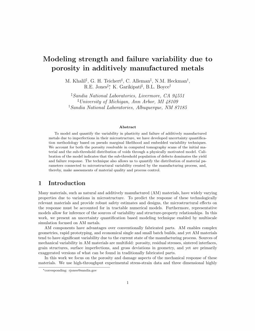
All the tensile tests were performed at a 10−3/s strain rate effected by grips engaging thedovetail ends of the specimen seen in the inset of Fig. 1. Engineering stress was measured with aload cell, the cross-section measured by CT and optical techniques, and the strain was determinedby digital image correlation (DIC) of the gauge section. Fig. 1 illustrates the ensemble of tensiletests which display variation in their elastic response, yield and hardening behavior, and failurecharacteristics. Clearly, the variability tends to increase across the ensemble from the elastic to thefailure regime. From these experimental stress-strain curves we extracted a number of QoIs, F : theeffective elastic modulus E from the initial slope, the yield strength σY from a 0.001 offset straincriterion, the yield strain εY from the strain corresponding to the yield stress, the ultimate tensilestrength σU from the maximum stress, the ultimate tensile strain εU from the strain correspondingto the maximum stress, the failure strain εf from maximum strain achieved, and the failure stressσf stress corresponding to maximum strain. Model calibration described in Sec.4 utilized this data,

4

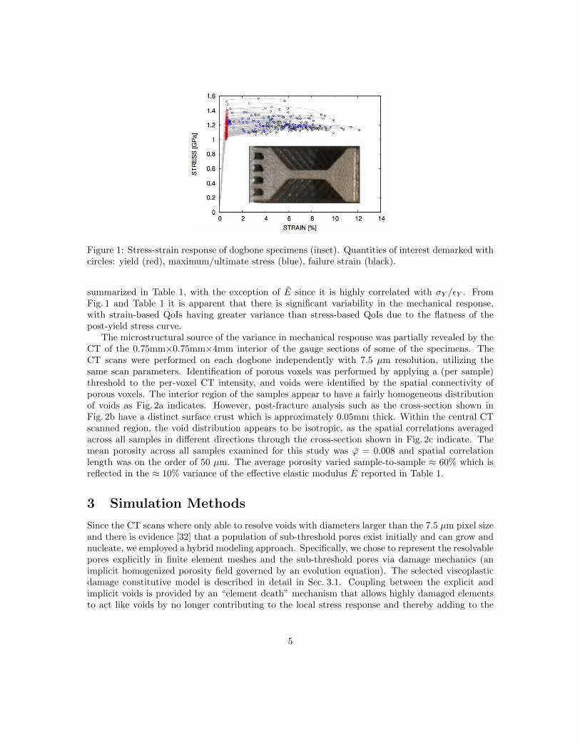
Figure 1: Stress-strain response of dogbone specimens (inset). Quantities of interest demarked withcircles: yield (red), maximum/ultimate stress (blue), failure strain (black).

summarized in Table 1, with the exception of E since it is highly correlated with σY /εY . FromFig. 1 and Table 1 it is apparent that there is significant variability in the mechanical response,with strain-based QoIs having greater variance than stress-based QoIs due to the flatness of thepost-yield stress curve.

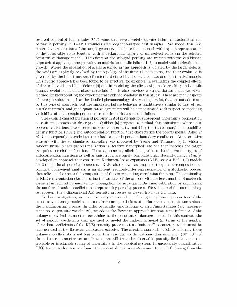
The microstructural source of the variance in mechanical response was partially revealed by theCT of the 0.75mm×0.75mm×4mm interior of the gauge sections of some of the specimens. TheCT scans were performed on each dogbone independently with 7.5 µm resolution, utilizing thesame scan parameters. Identification of porous voxels was performed by applying a (per sample)threshold to the per-voxel CT intensity, and voids were identified by the spatial connectivity ofporous voxels. The interior region of the samples appear to have a fairly homogeneous distributionof voids as Fig. 2a indicates. However, post-fracture analysis such as the cross-section shown inFig. 2b have a distinct surface crust which is approximately 0.05mm thick. Within the central CTscanned region, the void distribution appears to be isotropic, as the spatial correlations averagedacross all samples in different directions through the cross-section shown in Fig. 2c indicate. Themean porosity across all samples examined for this study was ϕ = 0.008 and spatial correlationlength was on the order of 50 µm. The average porosity varied sample-to-sample ≈ 60% which isreflected in the ≈ 10% variance of the effective elastic modulus E reported in Table 1.

3 Simulation Methods

Since the CT scans where only able to resolve voids with diameters larger than the 7.5 µm pixel sizeand there is evidence [32] that a population of sub-threshold pores exist initially and can grow andnucleate, we employed a hybrid modeling approach. Specifically, we chose to represent the resolvablepores explicitly in finite element meshes and the sub-threshold pores via damage mechanics (animplicit homogenized porosity field governed by an evolution equation). The selected viscoplasticdamage constitutive model is described in detail in Sec. 3.1. Coupling between the explicit andimplicit voids is provided by an “element death” mechanism that allows highly damaged elementsto act like voids by no longer contributing to the local stress response and thereby adding to the

5

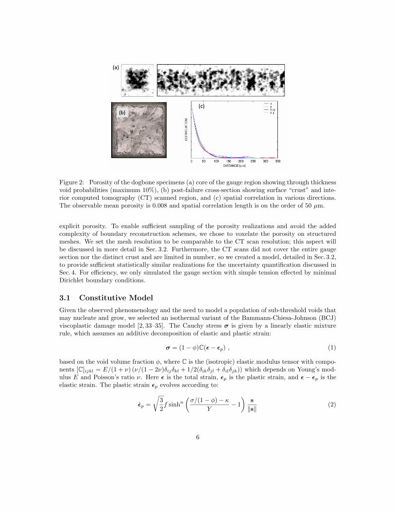
Figure 2: Porosity of the dogbone specimens (a) core of the gauge region showing through thicknessvoid probabilities (maximum 10%), (b) post-failure cross-section showing surface “crust” and inte-rior computed tomography (CT) scanned region, and (c) spatial correlation in various directions.The observable mean porosity is 0.008 and spatial correlation length is on the order of 50 µm.

explicit porosity. To enable sufficient sampling of the porosity realizations and avoid the addedcomplexity of boundary reconstruction schemes, we chose to voxelate the porosity on structuredmeshes. We set the mesh resolution to be comparable to the CT scan resolution; this aspect willbe discussed in more detail in Sec. 3.2. Furthermore, the CT scans did not cover the entire gaugesection nor the distinct crust and are limited in number, so we created a model, detailed in Sec.3.2,to provide sufficient statistically similar realizations for the uncertainty quantification discussed inSec. 4. For efficiency, we only simulated the gauge section with simple tension effected by minimalDirichlet boundary conditions.

3.1 Constitutive Model

Given the observed phenomenology and the need to model a population of sub-threshold voids thatmay nucleate and grow, we selected an isothermal variant of the Bammann-Chiesa-Johnson (BCJ)viscoplastic damage model [2, 33–35]. The Cauchy stress σ is given by a linearly elastic mixturerule, which assumes an additive decomposition of elastic and plastic strain:

σ = (1− φ)C(ε− εp) , (1)

based on the void volume fraction φ, where C is the (isotropic) elastic modulus tensor with compo-nents [C]ijkl = E/(1 + ν) (ν/(1− 2ν)δijδkl + 1/2(δikδjl + δilδjk)) which depends on Young’s mod-ulus E and Poisson’s ratio ν. Here ε is the total strain, εp is the plastic strain, and ε − εp is theelastic strain. The plastic strain εp evolves according to:

εp =

√3

2f sinhn

(σ/(1− φ)− κ

Y− 1

)s

‖s‖(2)

6

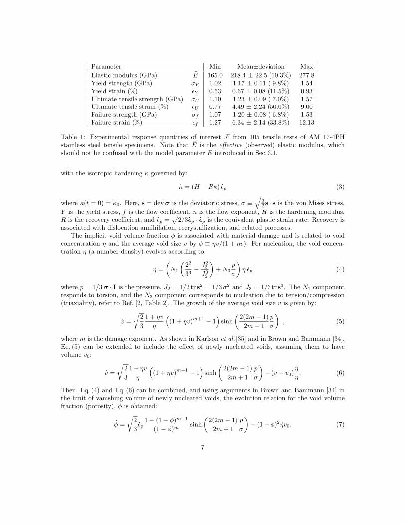
Parameter Min Mean±deviation Max

Elastic modulus (GPa) E 165.0 218.4 ± 22.5 (10.3%) 277.8Yield strength (GPa) σY 1.02 1.17 ± 0.11 ( 9.8%) 1.54Yield strain (%) εY 0.53 0.67 ± 0.08 (11.5%) 0.93Ultimate tensile strength (GPa) σU 1.10 1.23 ± 0.09 ( 7.0%) 1.57Ultimate tensile strain (%) εU 0.77 4.49 ± 2.24 (50.0%) 9.00Failure strength (GPa) σf 1.07 1.20 ± 0.08 ( 6.8%) 1.53Failure strain (%) εf 1.27 6.34 ± 2.14 (33.8%) 12.13

Table 1: Experimental response quantities of interest F from 105 tensile tests of AM 17-4PHstainless steel tensile specimens. Note that E is the effective (observed) elastic modulus, whichshould not be confused with the model parameter E introduced in Sec. 3.1.

with the isotropic hardening κ governed by:

κ = (H −Rκ) εp (3)

where κ(t = 0) = κ0. Here, s = devσ is the deviatoric stress, σ ≡√

32s · s is the von Mises stress,

Y is the yield stress, f is the flow coefficient, n is the flow exponent, H is the hardening modulus,R is the recovery coefficient, and εp =

√2/3εp · εp is the equivalent plastic strain rate. Recovery is

associated with dislocation annihilation, recrystallization, and related processes.The implicit void volume fraction φ is associated with material damage and is related to void

concentration η and the average void size v by φ ≡ ηv/(1 + ηv). For nucleation, the void concen-tration η (a number density) evolves according to:

η =

(N1

(22

33− J2

3

J32

)+N3

p

σ

)η εp (4)

where p = 1/3σ · I is the pressure, J2 = 1/2 tr s2 = 1/3σ2 and J3 = 1/3 tr s3. The N1 componentresponds to torsion, and the N3 component corresponds to nucleation due to tension/compression(triaxiality), refer to Ref. [2, Table 2]. The growth of the average void size v is given by:

v =

√2

3

1 + ηv

η

((1 + ηv)

m+1 − 1)

sinh

(2(2m− 1)

2m+ 1

p

σ

), (5)

where m is the damage exponent. As shown in Karlson et al. [35] and in Brown and Bammann [34],Eq. (5) can be extended to include the effect of newly nucleated voids, assuming them to havevolume v0:

v =

√2

3

1 + ηv

η

((1 + ηv)

m+1 − 1)

sinh

(2(2m− 1)

2m+ 1

p

σ

)− (v − v0)

η

η. (6)

Then, Eq. (4) and Eq. (6) can be combined, and using arguments in Brown and Bammann [34] inthe limit of vanishing volume of newly nucleated voids, the evolution relation for the void volumefraction (porosity), φ is obtained:

φ =

√2

3εp

1− (1− φ)m+1

(1− φ)msinh

(2(2m− 1)

2m+ 1

p

σ

)+ (1− φ)2ηv0. (7)

7

Lastly, once the void fraction φ exceeds a threshold φmax the material, as discretized by the finiteelement mesh, is considered completely failed.

3.2 Generation of Synthetic Microstructures

To develop models that are consistent with experimentally-observed failure metrics while accountingfor the resolvable porosity, we need a means of generating mesh-based realizations of the CT visibleporosity. Various approaches have previously been proposed in the literature to model randomlyporous media [6–8]. We used a Karhunen-Loeve expansion (KLE) (see e.g. Ref. [10]) to modelporous media as a random process through an intermediate Gaussian random process. KLE is amean-square optimal representation of square-integrable stochastic processes and has been widelyused in many engineering and scientific fields. Much like a Fourier series representation, KLErepresents a stochastic process using a linear combination of orthogonal functions; however, KLEdiffers from Fourier series in that the coefficients are random variables (as opposed to deterministicscalar quantities) and the basis depends on the correlation function of the process being modeled(as opposed to pre-specified harmonic functions).

Ilango et al. [9] proposed a methodology to construct KLE models (see App. A for a synopsisand generalization) for 2-dimensional porosity processes. Herein, we will extend the methodology toconstruct KLE models for the 3-dimensional porosity process of the core and crust regions such asthose visible in Fig. 2b. Given the experimental data, we assumed that the binary random processmodeling porosity ϕ(x) is homogeneous and isotropic [7, 36], with a two-point correlation functiongiven by

Rϕϕ (x1,x2) = E [ϕ(x1)ϕ(x2)] = Rϕϕ(r) (8)

where r = ‖x1 − x2‖ is the distance between positions x1 and x2.A modeling choice was made to construct one KLE model for the ensemble of specimens as

opposed to a separate KLE model for each dogbone sample. This choice was justified by the factthat the extracted empirical correlation function did not vary significantly across samples of thecore region (no data was available for the crust), and thus our aim was to represent the varianceof the physical response across an ensemble of structures produced under nominally identical con-ditions. With this choice, we approximated the statistics: mean porosity ϕ and spatial correlationRϕϕ, as ensemble averages utilizing the available CT scans across all samples of the porous mediaas described in Ref. [7]. The ensemble average was taken to be the average over all specimens andall available pairwise combinations of voxels and associated distances. The constructed KLE repre-sentation of ϕ(x) was subsequently used to generate realizations by sampling ϕ(x) on a structuredmesh covering the nominal gauge section of the tensile specimens and at a resolution commensuratewith the CT voxels. Specifically, we generated realizations of these processes on a structured gridof 135×135×534 voxels identical to the CT scan with 7.5µm pixel resolution, where the outer 10voxels in a cross-section were designated as the crust and the remainder as core.

Starting with the core region, we obtained a mean porosity of ϕ= 0.008 and Fig. 2c providesthe experimental correlation function Rϕϕ(r) as a function of distance r between voxels. There isnoise in the underlying experimental data which is predominantly attributed to (a) a finite sampleof specimens being analyzed and (b) the process of obtaining and post-processing CT images. Inorder to filter out this noise while satisfying physical constraints relating to correlation functions,we fit the data to the widely-used power-exponential correlation function [37,38]:

R(r) = exp(−( rκ

)ρ), (9)

8

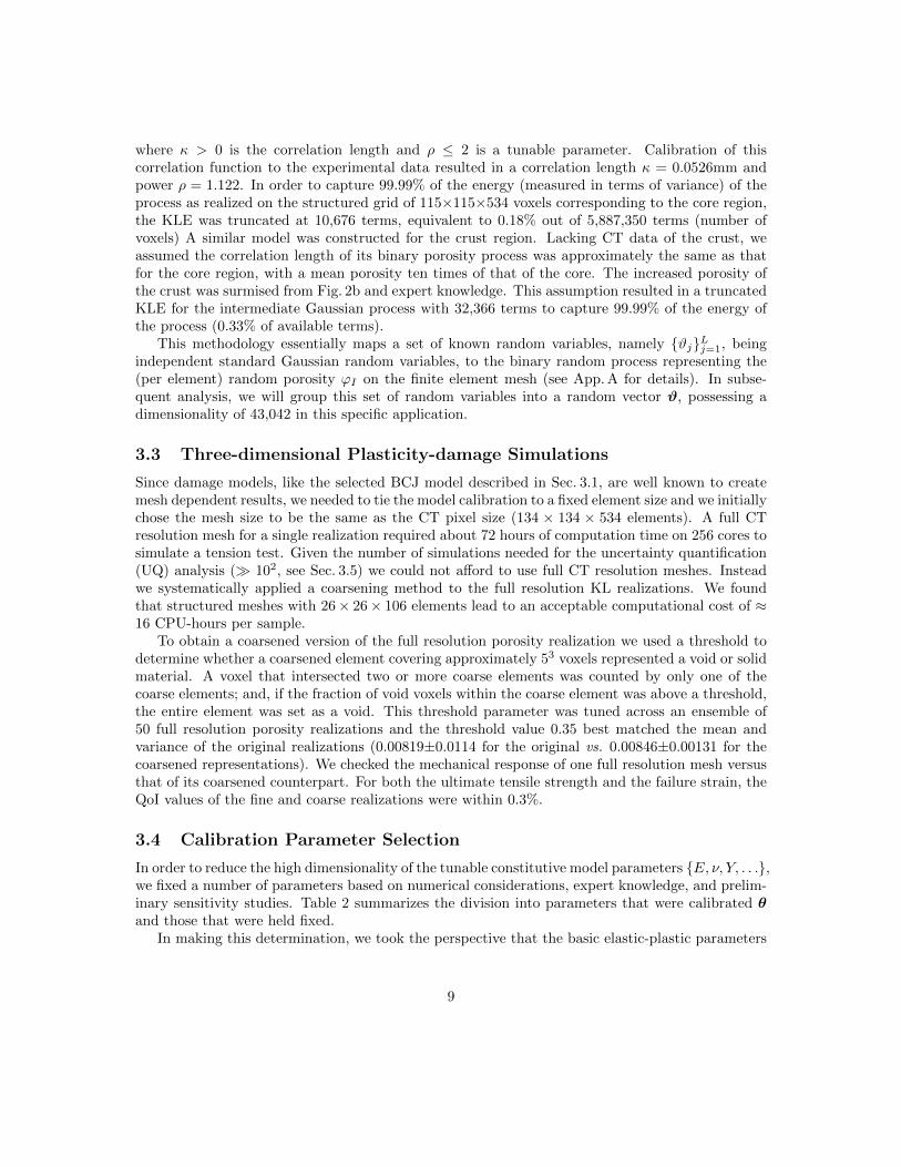
where κ > 0 is the correlation length and ρ ≤ 2 is a tunable parameter. Calibration of thiscorrelation function to the experimental data resulted in a correlation length κ = 0.0526mm andpower ρ = 1.122. In order to capture 99.99% of the energy (measured in terms of variance) of theprocess as realized on the structured grid of 115×115×534 voxels corresponding to the core region,the KLE was truncated at 10,676 terms, equivalent to 0.18% out of 5,887,350 terms (number ofvoxels) A similar model was constructed for the crust region. Lacking CT data of the crust, weassumed the correlation length of its binary porosity process was approximately the same as thatfor the core region, with a mean porosity ten times of that of the core. The increased porosity ofthe crust was surmised from Fig. 2b and expert knowledge. This assumption resulted in a truncatedKLE for the intermediate Gaussian process with 32,366 terms to capture 99.99% of the energy ofthe process (0.33% of available terms).

This methodology essentially maps a set of known random variables, namely ϑjLj=1, beingindependent standard Gaussian random variables, to the binary random process representing the(per element) random porosity ϕI on the finite element mesh (see App. A for details). In subse-quent analysis, we will group this set of random variables into a random vector ϑ, possessing adimensionality of 43,042 in this specific application.

3.3 Three-dimensional Plasticity-damage Simulations

Since damage models, like the selected BCJ model described in Sec. 3.1, are well known to createmesh dependent results, we needed to tie the model calibration to a fixed element size and we initiallychose the mesh size to be the same as the CT pixel size (134 × 134 × 534 elements). A full CTresolution mesh for a single realization required about 72 hours of computation time on 256 cores tosimulate a tension test. Given the number of simulations needed for the uncertainty quantification(UQ) analysis ( 102, see Sec. 3.5) we could not afford to use full CT resolution meshes. Insteadwe systematically applied a coarsening method to the full resolution KL realizations. We foundthat structured meshes with 26× 26× 106 elements lead to an acceptable computational cost of ≈16 CPU-hours per sample.

To obtain a coarsened version of the full resolution porosity realization we used a threshold todetermine whether a coarsened element covering approximately 53 voxels represented a void or solidmaterial. A voxel that intersected two or more coarse elements was counted by only one of thecoarse elements; and, if the fraction of void voxels within the coarse element was above a threshold,the entire element was set as a void. This threshold parameter was tuned across an ensemble of50 full resolution porosity realizations and the threshold value 0.35 best matched the mean andvariance of the original realizations (0.00819±0.0114 for the original vs. 0.00846±0.00131 for thecoarsened representations). We checked the mechanical response of one full resolution mesh versusthat of its coarsened counterpart. For both the ultimate tensile strength and the failure strain, theQoI values of the fine and coarse realizations were within 0.3%.

3.4 Calibration Parameter Selection

In order to reduce the high dimensionality of the tunable constitutive model parameters E, ν, Y, . . .,we fixed a number of parameters based on numerical considerations, expert knowledge, and prelim-inary sensitivity studies. Table 2 summarizes the division into parameters that were calibrated θand those that were held fixed.

In making this determination, we took the perspective that the basic elastic-plastic parameters

9

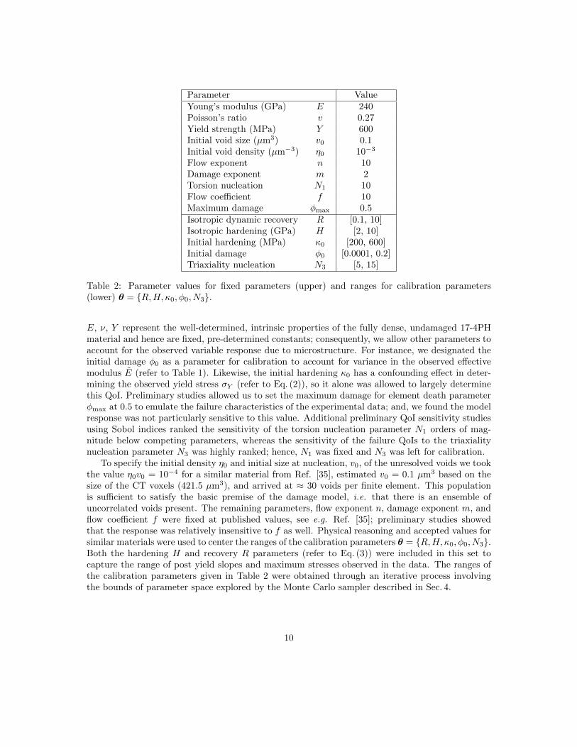
Parameter ValueYoung’s modulus (GPa) E 240Poisson’s ratio v 0.27Yield strength (MPa) Y 600Initial void size (µm3) v0 0.1Initial void density (µm−3) η0 10−3

Flow exponent n 10Damage exponent m 2Torsion nucleation N1 10Flow coefficient f 10Maximum damage φmax 0.5Isotropic dynamic recovery R [0.1, 10]Isotropic hardening (GPa) H [2, 10]Initial hardening (MPa) κ0 [200, 600]Initial damage φ0 [0.0001, 0.2]Triaxiality nucleation N3 [5, 15]

Table 2: Parameter values for fixed parameters (upper) and ranges for calibration parameters(lower) θ = R,H, κ0, φ0, N3.

E, ν, Y represent the well-determined, intrinsic properties of the fully dense, undamaged 17-4PHmaterial and hence are fixed, pre-determined constants; consequently, we allow other parameters toaccount for the observed variable response due to microstructure. For instance, we designated theinitial damage φ0 as a parameter for calibration to account for variance in the observed effectivemodulus E (refer to Table 1). Likewise, the initial hardening κ0 has a confounding effect in deter-mining the observed yield stress σY (refer to Eq. (2)), so it alone was allowed to largely determinethis QoI. Preliminary studies allowed us to set the maximum damage for element death parameterφmax at 0.5 to emulate the failure characteristics of the experimental data; and, we found the modelresponse was not particularly sensitive to this value. Additional preliminary QoI sensitivity studiesusing Sobol indices ranked the sensitivity of the torsion nucleation parameter N1 orders of mag-nitude below competing parameters, whereas the sensitivity of the failure QoIs to the triaxialitynucleation parameter N3 was highly ranked; hence, N1 was fixed and N3 was left for calibration.

To specify the initial density η0 and initial size at nucleation, v0, of the unresolved voids we tookthe value η0v0 = 10−4 for a similar material from Ref. [35], estimated v0 = 0.1 µm3 based on thesize of the CT voxels (421.5 µm3), and arrived at ≈ 30 voids per finite element. This populationis sufficient to satisfy the basic premise of the damage model, i.e. that there is an ensemble ofuncorrelated voids present. The remaining parameters, flow exponent n, damage exponent m, andflow coefficient f were fixed at published values, see e.g. Ref. [35]; preliminary studies showedthat the response was relatively insensitive to f as well. Physical reasoning and accepted values forsimilar materials were used to center the ranges of the calibration parameters θ = R,H, κ0, φ0, N3.Both the hardening H and recovery R parameters (refer to Eq. (3)) were included in this set tocapture the range of post yield slopes and maximum stresses observed in the data. The ranges ofthe calibration parameters given in Table 2 were obtained through an iterative process involvingthe bounds of parameter space explored by the Monte Carlo sampler described in Sec. 4.

10

3.5 Response Surrogate Model

To calibrate likely values for the parameters θ given the experimental data, we used Bayesian modelcalibration techniques developed in Sec. 4. This statistical inversion relies on the joint samplingof the posterior PDF of the parameters θ using Markov chain Monte Carlo (MCMC) sampling-based strategies. The joint characterization of the posterior parameter PDF of 5 independentparameters usually requires at least 106 samples (at 16 CPU-hours per sample), where each sampleis a forward model simulation of the computationally-intensive finite element model described inSec. 3.3. One popular strategy that reduces this computational burden relies on surrogate modelsof the physical response. Such surrogates capture the complex, often nonlinear, mapping from theunknown parameters θ to observable, system QoIs F . Although not general purpose, QoI surrogatemodels are designed to be relatively cheap to evaluate while being of sufficient accuracy.

Following the strategy used in in a previous study [26], we first attempted to employ a poly-nomial chaos expansion (PCE) [39, 40] to construct surrogates over the domain of plausible valuesof the unknown parameters. Such a methodology exploits a global polynomial basis for captur-ing nonlinear input-output mappings (as exhibited by the response surfaces for the observed QoIsin Fig. 4). Specifically, PCE surrogates require higher-order bases to capture the nonlinearitiesaccurately. This implies an exponential growth in the number of unknown PCE coefficients totune, which is proportional to the number of forward model simulations required to construct suchsurrogates. For this work, we first attempted the construction of third-order PCE surrogates inthe 5-dimensional parameter space. The PCE coefficients were obtained using Galerkin projectionutilizing 241 simulations corresponding to quadrature points obtained using Smolyak’s sparse ten-sorization and the nested Clenshaw-Curtis quadrature formula [10]. The accuracy, as measuredusing normalized root-mean-square error with 100 additional simulations corresponding to MonteCarlo samples, was deemed insufficient for subsequent calibration tasks. Such surrogates also ex-hibited slow convergence against increasing PCE order from 1 through 3. In such situations, onemay attempt to construct higher order PCE surrogates, but a 4th order PCE surrogate wouldhave required a prohibitive 801 sparse-quadrature points (simulations) for construction. Given theunacceptable computational cost of pursuing this approach, we decided to abandon the PCE-basedapproach, and to turn to an approach using radial basis functions (RBF’s) [41–43].

Specifically, we used RBF’s to construct surrogate response models for each physical QoI F asa function of the calibration parameters θ, since they are one of the most capable multidimensionalapproximation methods [44]. For each porosity realization constructed using the methodologyoutlined in Sec.3.2, we fit a RBF surrogate for each of the 6 QoIs F reported in Table 1. One couldconstruct a global surrogate (over all realizations) per QoI to cover the space of KLE coefficientsused in modeling the explicit porosity process as well as the unknown parameters, but we optedagainst that approach due to the extremely high-dimensionality of the KLE coefficient space (seeSec.3.2 for details). Instead, we constructed surrogate models for the observed QoIs in terms of onlythe unknown parameters over a finite number of porosity realizations (one surrogate per QoI for aspecific porosity realization), with the number of porosity realizations (< 100) being significantlylower than the dimensionality of the porosity process (> 10,000). To construct such approximations,we started with a set of parameter points θi, i = 1, . . . , n, and corresponding QoI values, fi = f (θi)for each QoI fi in F .

The RBF approximation, f ≈ f (θ), is a linear combination of basis functions (kernels) thatdepend on the distances between the evaluation point, θ, and a set of kernel centers, θJ , J =

11

1, . . . ,M given by

f (θ) =

M∑J=1

cJK (‖θ − θJ‖) (10)

where ‖·‖ denotes the Euclidean norm, and coefficients cJ are to be determined. Widely-used kernels

include Gaussian, K (r) = e−(εr)2 , multiquadratic, K (r) =

√1 + (εr)

2, and cubic, K (r) = εr3,

where ε is a tunable shape parameter (see Ref. [45] for a more complete list of RBF kernels). Afterpreliminary comparative investigations (results omitted for brevity), we chose to utilize Gaussiankernels, since they lead to sufficiently-low cross-validation errors in this context. Regarding thechoice of shape parameter ε, there exist many rules of thumb as well as data-driven approaches (seeRef. [46] for a brief survey). For simplicity, we chose to use the value of D/

√M as recommended

by Franke [47], with D representing the diameter of the smallest hypersphere containing all datapoints. Since we work with normalized parameters in the range of [−1, 1], D is then equal to 2

√np,

with np = 5 being the dimensionality of the parameter space θ. A quick sensitivity study yieldedno significant increase in accuracy of the resulting surrogates with varying choice of ε about thisrecommended value.

In many applications, the centers θJ are chosen to be the data points θJ = θi, withM = n. The constants cJ , in that setting, may be determined by having the approximationexactly match the given data at the data points, leading to an interpolative approximation functionbased on collocation. In this realistic application, the QoIs extracted from the simulations werecorrupted by relatively small, yet significant, noise relating to errors in the QoI-extraction fromstress-strain curves sampled at a finite set of strain values. In other words, the true value fi = f (θi),corresponding to parameter realization θi, was known only up to a small amount of unknown noise.In this case, an interpolative RBF approximation is equivalent to fitting the unknown noise alongwith the underlying QoI. More generally, over-fitting leads to erroneous surrogates even in thenoise-free case due to parameter identifiability issues.

The issue of over-fitting the noise in the extracted QoIs may be alleviated through regularization[48], for example. We reduced the effect of noise by choosing the number of centers to be less thanthe number of available data points, i.e. M < n, as form of projection. An advantage of this choiceis the reduced cost in evaluating the trained RBF surrogates. The specific number of centers Mis a modeling choice that was made using cross-validation, with the leave-one-out cross-validation(LOOCV) error available in closed-form [49]. The locations of both sets of data points and centersfor RBF surrogate construction were obtained using Latin hypercube sampling (LHS) [50], resultingin a sample set that was predominantly random, but uniform in each separate dimension. Althoughmore optimal strategies exist for choosing the data points and centers adaptively (see Ref. [51] forexample), we chose this space-filling design.

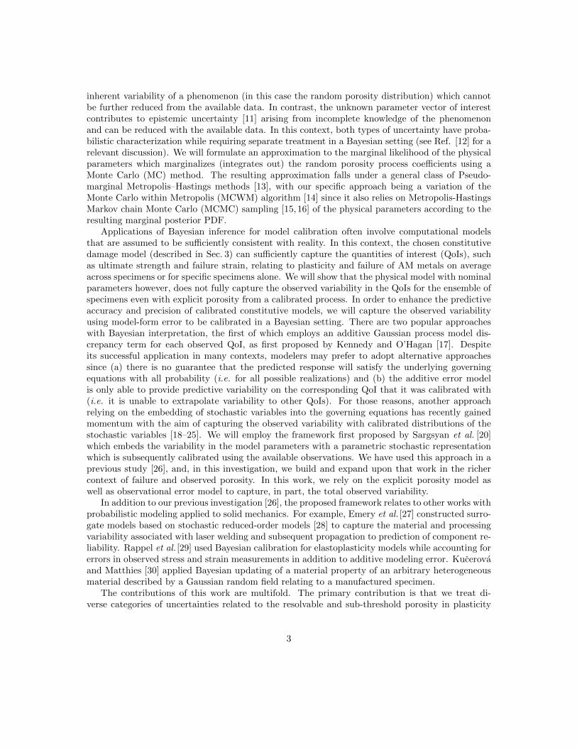
To obtain data at points θi for each porosity realization, we ran n = 200 forward modelsimulations at a set of corresponding LHS samples in parameter space with parameter ranges givenin Table 2. The extracted QoIs Fi from those simulations were used in training the RBF surrogates.We varied the number of RBF centers θJ , J = 1, . . .M using M from 20 to 80, and extracted theLOOCV error for each trained RBF surrogate. To obtain the average LOOCV error, normalizedby the corresponding QoI, the process was repeated over the 50 available porosity realizations, anda further 30 times (per porosity realization) over different LHS realizations of the centers. Theresults are shown in Fig. 3. Overall, a choice of M = 50 centers results in RBF surrogates withclose to minimal error for all QoIs, an increase in M results in negligible reduction in the LOOCVerror for some QoIs and a substantial increase in error for the noisier QoIs εU and εf .

12

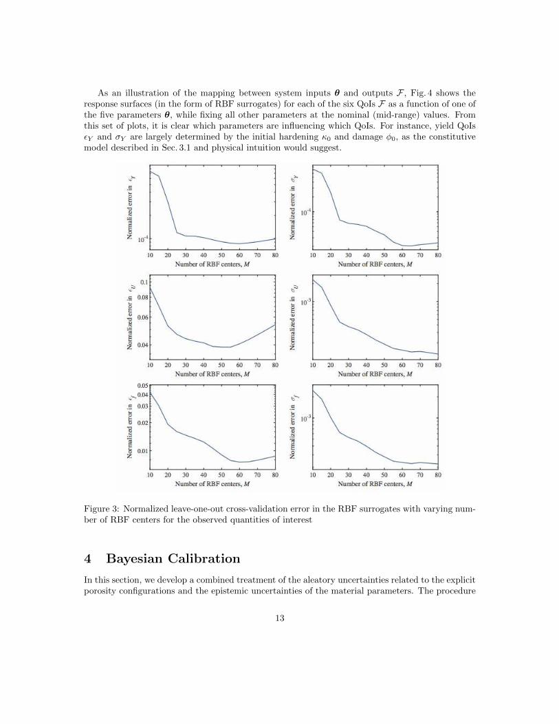
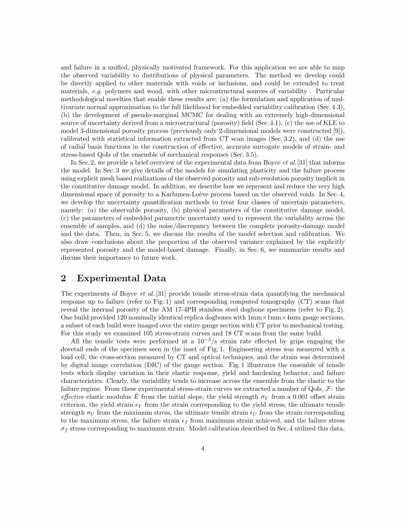
As an illustration of the mapping between system inputs θ and outputs F , Fig. 4 shows theresponse surfaces (in the form of RBF surrogates) for each of the six QoIs F as a function of one ofthe five parameters θ, while fixing all other parameters at the nominal (mid-range) values. Fromthis set of plots, it is clear which parameters are influencing which QoIs. For instance, yield QoIsεY and σY are largely determined by the initial hardening κ0 and damage φ0, as the constitutivemodel described in Sec. 3.1 and physical intuition would suggest.

Figure 3: Normalized leave-one-out cross-validation error in the RBF surrogates with varying num-ber of RBF centers for the observed quantities of interest

4 Bayesian Calibration

In this section, we develop a combined treatment of the aleatory uncertainties related to the explicitporosity configurations and the epistemic uncertainties of the material parameters. The procedure

13

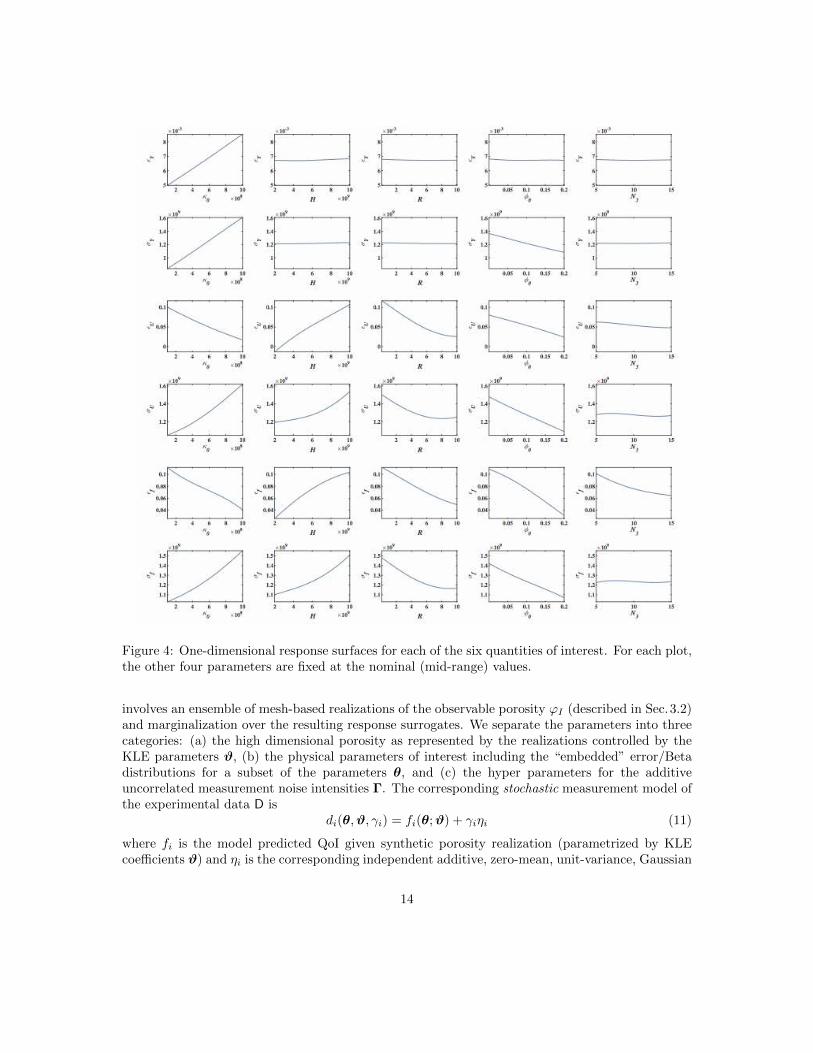
Figure 4: One-dimensional response surfaces for each of the six quantities of interest. For each plot,the other four parameters are fixed at the nominal (mid-range) values.

involves an ensemble of mesh-based realizations of the observable porosity ϕI (described in Sec.3.2)and marginalization over the resulting response surrogates. We separate the parameters into threecategories: (a) the high dimensional porosity as represented by the realizations controlled by theKLE parameters ϑ, (b) the physical parameters of interest including the “embedded” error/Betadistributions for a subset of the parameters θ, and (c) the hyper parameters for the additiveuncorrelated measurement noise intensities Γ. The corresponding stochastic measurement model ofthe experimental data D is

di(θ,ϑ, γi) = fi(θ;ϑ) + γiηi (11)

where fi is the model predicted QoI given synthetic porosity realization (parametrized by KLEcoefficients ϑ) and ηi is the corresponding independent additive, zero-mean, unit-variance, Gaussian

14

noise, scaled by parameter γi. We can rewrite Eq. (11) in vector format, grouping all observed QoIsand model-predicted counterparts into vectors d and F , respectively, to obtain

d(θ,ϑ,Γ) = F(θ;ϑ) + Γη , (12)

with Γ denoting the diagonal matrix with the diagonal elements Γi,i = γi, and η being the vectorof identical independently distributed (IID) zero-mean, unit-variance, Gaussian random variables

ηi. The available data D is comprised of the six QoIs d(j) = F (i) (see Table 1) as extracted from105 tensile tests (j = 1, . . . , 105), one per available AM dogbone specimen.

4.1 Inference in the Presence of High-Dimensional Aleatory Uncertainty:Pseudo-Marginal Likelihood Approach

Generally speaking, the statistical calibration of models using experimental data involves inferringa set of unknown, or weakly known, parameters. Often, a subset of those parameters are notdirectly relevant for subsequent analysis (such as sensitivity analysis or forward propagation ofuncertainty). Such parameters, generally termed “nuisance” parameters, are still important in thecalibration process and are thus jointly inferred with the parameters of interest. The parametersγi scaling the measurement noise ηi are a common example of this kind of parameter.

In this section, we describe how we deal with a different kind of nuisance parameter vector, ϑ,which is used to model (via Karhunen-Loeve expansion described in Sec. 3.2) the high-dimensionalrandom process. This is the observable porosity field ϕ(x), which acts as an uncontrollable sourceof uncertainty in the physical system, i.e. the location and sizes of voids. In UQ terms, such asource of uncertainty contributes to aleatory uncertainty [11], arising from the inherent variabilityof a phenomenon (in this case the random porosity distribution) which cannot be further reducedfrom the available data. Here, this means that we cannot rely on knowing the locations of voidswhen making predictions. In contrast, the unknown parameter vector θ of interest contributesto epistemic uncertainty [11] arising from incomplete knowledge of the phenomenon and can bereduced with the available data D. In this context, both types of uncertainty have probabilisticcharacterization. However, modelers utilizing UQ techniques make this distinction as the two typesof uncertainties require separate treatment in a Bayesian setting (see Ref. [12] for a philosophicaldiscussion on the need to separate sources of uncertainties in this fashion).

In such a setting, one performs joint inference of the uncertain parameters and nuisance param-eters. The joint posterior PDF of the uncertain parameter vector θ and nuisance parameter vectorϑ is first decomposed using Bayes’ law:

p (θ,ϑ |D) ∝ p (D |θ, ϑ) p (θ, ϑ) , (13)

with the first and second right-hand-side terms corresponding to the joint likelihood and priorPDFs of the vectors θ and ϑ, respectively. We proceed by inferring the marginal posterior PDFof θ, instead of joint inference of θ along with ϑ. Since ϑ is of high dimensionality (more than43,000 dimensions) in comparison to θ (5-dimensional), we marginalize over ϑ using a few MonteCarlo realizations (50 samples) distributed according to the marginal prior PDF, p (ϑ), of ϑ. Thisallows us to construct surrogate models for the observed QoIs in terms of θ over a limited num-ber of realizations of ϑ, and thus significantly reduce the computational cost involved in forwardmodel simulations. The other justification for this marginalization-based approach is the lack ofrequirement for a joint uncertain characterization of θ and ϑ since, as described, ϑ parametrizes

15

an uncontrollable source of uncertainty in the physical system, i.e. the location and sizes of voidsacross different AM specimens, and, hence, is not a quantity of direct engineering design interest.Note that for subsequent uncertainty propagation analysis, we will utilize a marginal posterior PDFof θ derived with this approach.

Towards that end, we first rewrite Eq. (13) as

p (θ,ϑ |D) ∝ p (D |θ, ϑ) p (θ) p (ϑ) , (14)

which assumes θ and ϑ are independent prior to the assimilation of data. (Given the lack ofprevious analysis/knowledge for a joint characterization this is a reasonable assumption to be madein practice.) Consequently, the marginal posterior PDF of θ is

p (θ |D) ∝[∫

p (D |θ, ϑ) p (ϑ) dϑ

]p (θ) . (15)

The integral in Eq. (15) corresponds to the marginal likelihood of θ, being the likelihood of θ aver-aged over ϑ, weighted by the prior PDF of ϑ, p (ϑ). In general, this marginal likelihood PDF doesnot have an analytical solution and one must resort to deterministic or stochastic schemes of numer-ical integration. One conceptually simple approach utilizes Monte Carlo (stochastic) integration toarrive at the following approximation p (θ |D) for the marginal posterior:

p (θ |D) ∝

1

NMC

NMC∑k=1

p (D |θ,ϑk)

p (θ) , (16)

with p (D |θ,ϑk) being the likelihood of the parameter vector θ conditional on the specific realizationof nuisance parameter vector ϑk and those realizations are distributed according to the prior PDFp (ϑ). For subsequent sampling of θ according to the approximate posterior PDF in Eq. (16),p (θ |D), we rely on adaptive Metropolis-Hastings Markov chain Monte Carlo (MCMC) sampling[15, 16]. In this context, the Monte Carlo approximation to the marginal likelihood falls undera general class of Pseudo-marginal Metropolis–Hastings methods [13], with our specific approachbeing a variation of the Monte Carlo within Metropolis (MCWM) algorithm [14]. More specifically,our variant of MCWM (suggested but not pursued in Ref. [13]) relies on the same set of realizationsof ϑ to compute the marginal likelihood for all samples of θ as generated by the MCMC simulation.This allows us to construct and reuse surrogates over a fixed ensemble of ϑ, namely ϑk, k =1, . . . , N

MC, corresponding to KLE realizations of the porosity process (obtained using Monte Carlo

sampling of KLE coefficients).In the next section, we will fully investigate the convergence properties of this pseudo-marginal

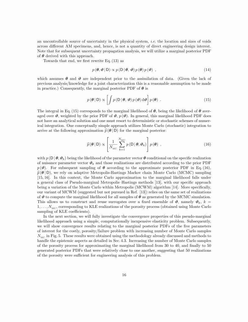
likelihood approach using a simple, computationally inexpensive elasticity problem. Subsequently,we will show convergence results relating to the marginal posterior PDFs of the five parametersof interest for the costly, porosity/failure problem with increasing number of Monte Carlo samplesN

MCin Fig. 5. These results were obtained using the methodology already discussed and methods to

handle the epistemic aspects as detailed in Sec. 4.3. Increasing the number of Monte Carlo samplesof the porosity process for approximating the marginal likelihood from 30 to 40, and finally to 50generated posterior PDFs that were relatively close to one another, suggesting that 50 realizationsof the porosity were sufficient for engineering analysis of this problem.

16

Figure 5: Parameter PDFs. Convergence with increasing number of realizations of the porosity formarginal likelihood computation.

4.2 Demonstrative Mechanics Example of the Pseudo-Marginal Likeli-hood Approach

To analyze the convergence properties of the Pseudo-Marginal Likelihood approach in a tractableway, we consider the following governing stochastic partial differential equation (SPDE) describingthe one-dimensional axial deformation of a rod [52] with stochastic geometry

∂

∂x

[EA (x;ϑ)

∂u

∂x

]+ f (x) = 0 , x ∈ Ω := (0, 1)

u (0) = u (1) = 0 , (17)

f (x) = 1 ,

with u being the displacement due to deformation, f being the axially-applied distributed force,E being the elastic modulus, and A being the stochastic, spatially-varying cross-sectional area(inducing heterogeneity) determined by the vector of KLE coefficients ϑ (introduced in Sec. 3.2).

Treating this as an inverse problem, we take the parameter E to be an unknown quantity tobe inferred from a set of 10 noisy observations of the mid-span deflection (i.e. u(x = 1/2), one perdifferent random realization of A(x) (i.e. a total of 10 repeated experiments). The observationalnoise is assumed to be independent and identically distributed (IID) Gaussian with zero mean andvariance of 5 × 10−7 (in comparison to an average mid-span deflection of 1.25 × 10−5). We willdiscretize Eq. (17) using the finite-element method (FEM) with 200 linear finite elements, whichproves sufficient resolution to represent the KLE modes. The stochastic cross-sectional area A(x;ϑ)is modeled as a log-normal random process, i.e.

A (x;ϑ) = A [1 + εα (x,ϑ)] , (18)

where A = 0.01 is the mean cross-sectional area, ε is the coefficient of variation, and α is a log-normalprocess:

α (x,ϑ) =1√

e (e− 1)exp

(g (x,ϑ)− e 1

2

), (19)

with zero mean and unit variance. Here, g (x,ϑ) is a zero-mean, unit-variance Gaussian stochasticprocess with an exponential covariance function [10]:

E [g (x, ·) g (x′, ·)] = exp

(−|x− x

′|b

), (20)

where b is the correlation length of the underlying Gaussian random process. Such choice of covari-ance function is convenient in this setting as it leads to analytical expressions for the eigenvalues

17

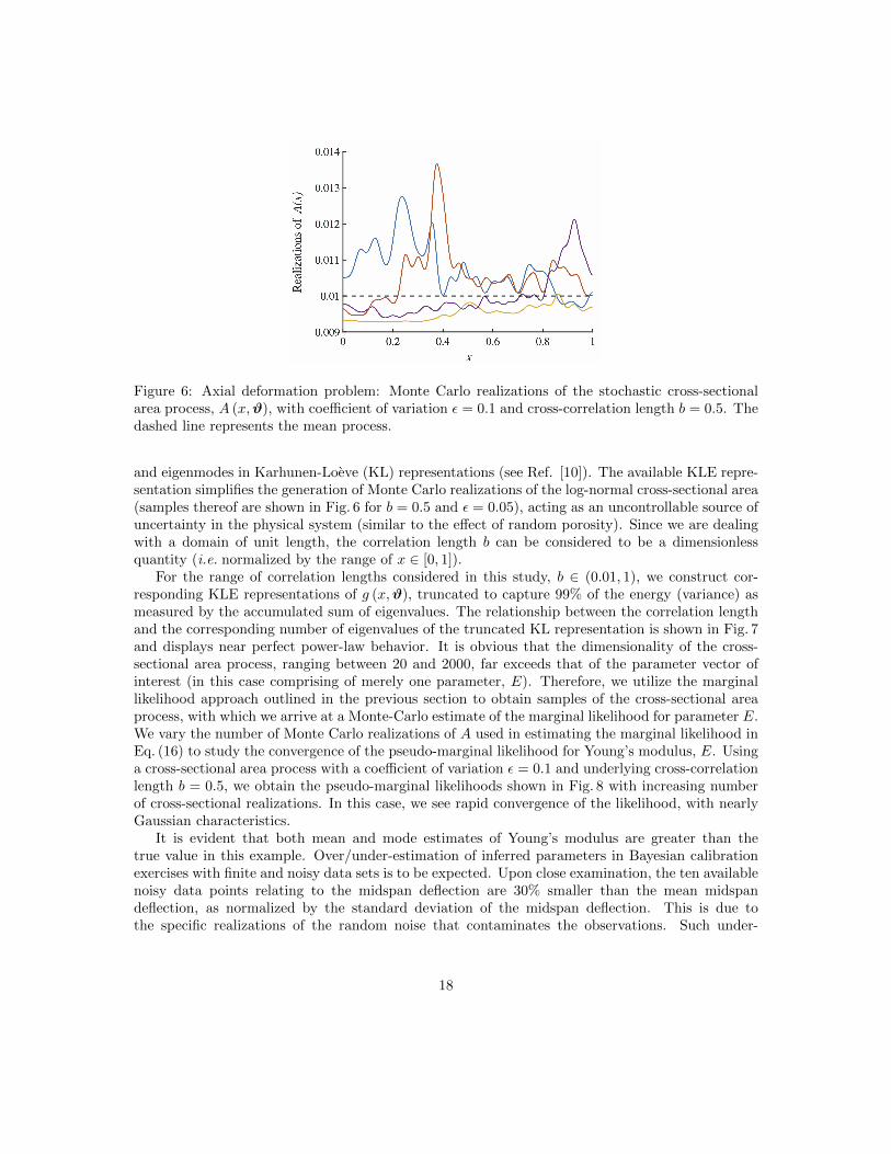
Figure 6: Axial deformation problem: Monte Carlo realizations of the stochastic cross-sectionalarea process, A (x,ϑ), with coefficient of variation ε = 0.1 and cross-correlation length b = 0.5. Thedashed line represents the mean process.

and eigenmodes in Karhunen-Loeve (KL) representations (see Ref. [10]). The available KLE repre-sentation simplifies the generation of Monte Carlo realizations of the log-normal cross-sectional area(samples thereof are shown in Fig. 6 for b = 0.5 and ε = 0.05), acting as an uncontrollable source ofuncertainty in the physical system (similar to the effect of random porosity). Since we are dealingwith a domain of unit length, the correlation length b can be considered to be a dimensionlessquantity (i.e. normalized by the range of x ∈ [0, 1]).

For the range of correlation lengths considered in this study, b ∈ (0.01, 1), we construct cor-responding KLE representations of g (x,ϑ), truncated to capture 99% of the energy (variance) asmeasured by the accumulated sum of eigenvalues. The relationship between the correlation lengthand the corresponding number of eigenvalues of the truncated KL representation is shown in Fig. 7and displays near perfect power-law behavior. It is obvious that the dimensionality of the cross-sectional area process, ranging between 20 and 2000, far exceeds that of the parameter vector ofinterest (in this case comprising of merely one parameter, E). Therefore, we utilize the marginallikelihood approach outlined in the previous section to obtain samples of the cross-sectional areaprocess, with which we arrive at a Monte-Carlo estimate of the marginal likelihood for parameter E.We vary the number of Monte Carlo realizations of A used in estimating the marginal likelihood inEq. (16) to study the convergence of the pseudo-marginal likelihood for Young’s modulus, E. Usinga cross-sectional area process with a coefficient of variation ε = 0.1 and underlying cross-correlationlength b = 0.5, we obtain the pseudo-marginal likelihoods shown in Fig. 8 with increasing numberof cross-sectional realizations. In this case, we see rapid convergence of the likelihood, with nearlyGaussian characteristics.

It is evident that both mean and mode estimates of Young’s modulus are greater than thetrue value in this example. Over/under-estimation of inferred parameters in Bayesian calibrationexercises with finite and noisy data sets is to be expected. Upon close examination, the ten availablenoisy data points relating to the midspan deflection are 30% smaller than the mean midspandeflection, as normalized by the standard deviation of the midspan deflection. This is due tothe specific realizations of the random noise that contaminates the observations. Such under-

18

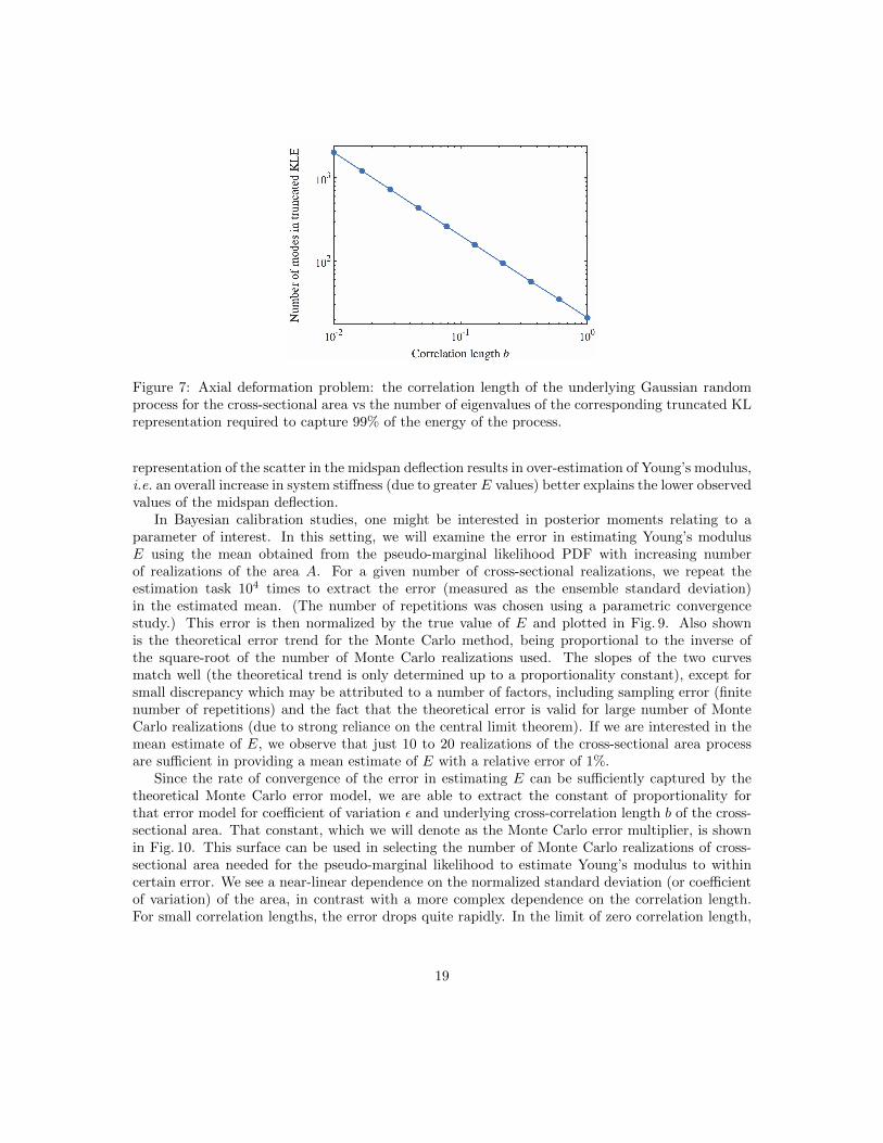
Figure 7: Axial deformation problem: the correlation length of the underlying Gaussian randomprocess for the cross-sectional area vs the number of eigenvalues of the corresponding truncated KLrepresentation required to capture 99% of the energy of the process.

representation of the scatter in the midspan deflection results in over-estimation of Young’s modulus,i.e. an overall increase in system stiffness (due to greater E values) better explains the lower observedvalues of the midspan deflection.

In Bayesian calibration studies, one might be interested in posterior moments relating to aparameter of interest. In this setting, we will examine the error in estimating Young’s modulusE using the mean obtained from the pseudo-marginal likelihood PDF with increasing numberof realizations of the area A. For a given number of cross-sectional realizations, we repeat theestimation task 104 times to extract the error (measured as the ensemble standard deviation)in the estimated mean. (The number of repetitions was chosen using a parametric convergencestudy.) This error is then normalized by the true value of E and plotted in Fig. 9. Also shownis the theoretical error trend for the Monte Carlo method, being proportional to the inverse ofthe square-root of the number of Monte Carlo realizations used. The slopes of the two curvesmatch well (the theoretical trend is only determined up to a proportionality constant), except forsmall discrepancy which may be attributed to a number of factors, including sampling error (finitenumber of repetitions) and the fact that the theoretical error is valid for large number of MonteCarlo realizations (due to strong reliance on the central limit theorem). If we are interested in themean estimate of E, we observe that just 10 to 20 realizations of the cross-sectional area processare sufficient in providing a mean estimate of E with a relative error of 1%.

Since the rate of convergence of the error in estimating E can be sufficiently captured by thetheoretical Monte Carlo error model, we are able to extract the constant of proportionality forthat error model for coefficient of variation ε and underlying cross-correlation length b of the cross-sectional area. That constant, which we will denote as the Monte Carlo error multiplier, is shownin Fig. 10. This surface can be used in selecting the number of Monte Carlo realizations of cross-sectional area needed for the pseudo-marginal likelihood to estimate Young’s modulus to withincertain error. We see a near-linear dependence on the normalized standard deviation (or coefficientof variation) of the area, in contrast with a more complex dependence on the correlation length.For small correlation lengths, the error drops quite rapidly. In the limit of zero correlation length,

19

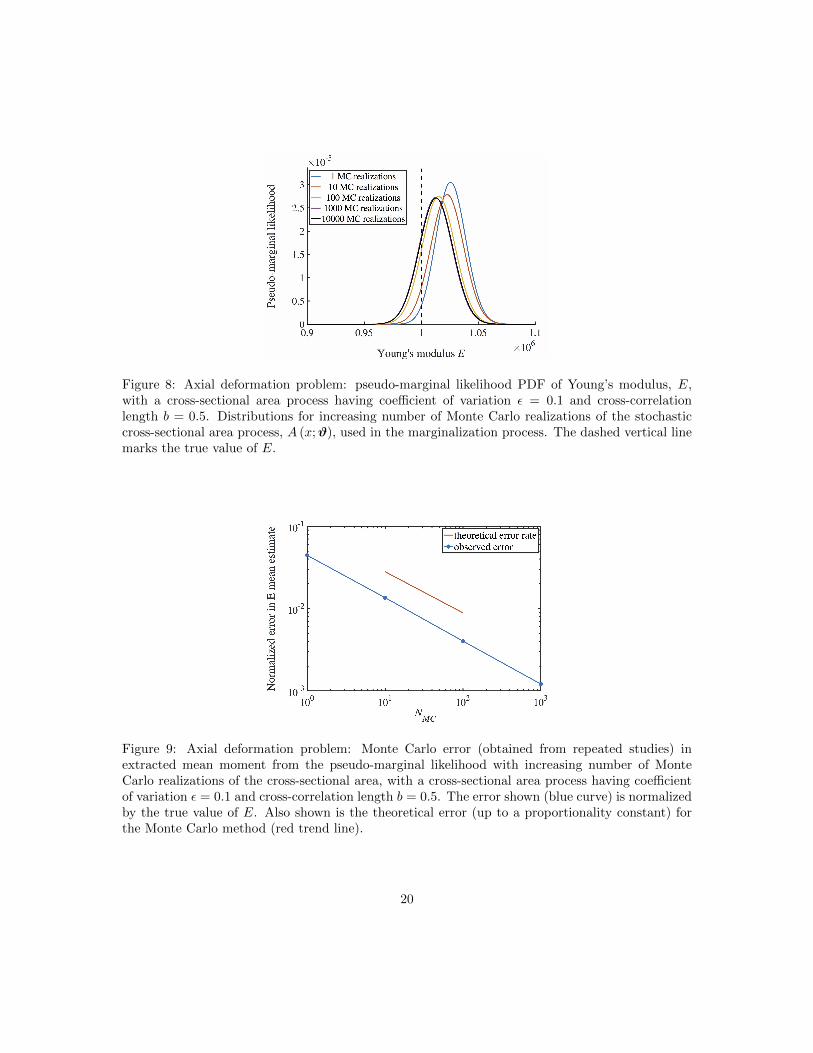
Figure 8: Axial deformation problem: pseudo-marginal likelihood PDF of Young’s modulus, E,with a cross-sectional area process having coefficient of variation ε = 0.1 and cross-correlationlength b = 0.5. Distributions for increasing number of Monte Carlo realizations of the stochasticcross-sectional area process, A (x;ϑ), used in the marginalization process. The dashed vertical linemarks the true value of E.

Figure 9: Axial deformation problem: Monte Carlo error (obtained from repeated studies) inextracted mean moment from the pseudo-marginal likelihood with increasing number of MonteCarlo realizations of the cross-sectional area, with a cross-sectional area process having coefficientof variation ε = 0.1 and cross-correlation length b = 0.5. The error shown (blue curve) is normalizedby the true value of E. Also shown is the theoretical error (up to a proportionality constant) forthe Monte Carlo method (red trend line).

20

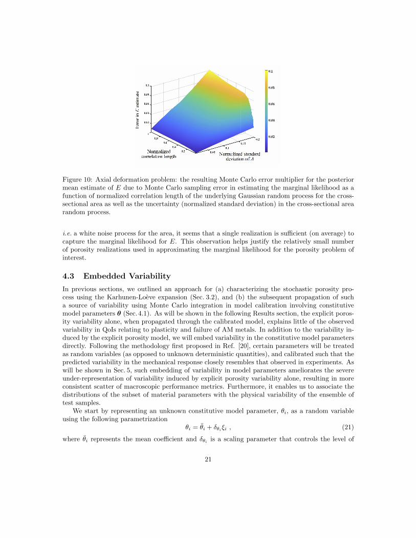
Figure 10: Axial deformation problem: the resulting Monte Carlo error multiplier for the posteriormean estimate of E due to Monte Carlo sampling error in estimating the marginal likelihood as afunction of normalized correlation length of the underlying Gaussian random process for the cross-sectional area as well as the uncertainty (normalized standard deviation) in the cross-sectional arearandom process.

i.e. a white noise process for the area, it seems that a single realization is sufficient (on average) tocapture the marginal likelihood for E. This observation helps justify the relatively small numberof porosity realizations used in approximating the marginal likelihood for the porosity problem ofinterest.

4.3 Embedded Variability

In previous sections, we outlined an approach for (a) characterizing the stochastic porosity pro-cess using the Karhunen-Loeve expansion (Sec. 3.2), and (b) the subsequent propagation of sucha source of variability using Monte Carlo integration in model calibration involving constitutivemodel parameters θ (Sec.4.1). As will be shown in the following Results section, the explicit poros-ity variability alone, when propagated through the calibrated model, explains little of the observedvariability in QoIs relating to plasticity and failure of AM metals. In addition to the variability in-duced by the explicit porosity model, we will embed variability in the constitutive model parametersdirectly. Following the methodology first proposed in Ref. [20], certain parameters will be treatedas random variables (as opposed to unknown deterministic quantities), and calibrated such that thepredicted variability in the mechanical response closely resembles that observed in experiments. Aswill be shown in Sec. 5, such embedding of variability in model parameters ameliorates the severeunder-representation of variability induced by explicit porosity variability alone, resulting in moreconsistent scatter of macroscopic performance metrics. Furthermore, it enables us to associate thedistributions of the subset of material parameters with the physical variability of the ensemble oftest samples.

We start by representing an unknown constitutive model parameter, θi, as a random variableusing the following parametrization

θi = θi + δθiξi , (21)

where θi represents the mean coefficient and δθi is a scaling parameter that controls the level of

21

variability of θi. Here, ξi is a zero-mean independent random variable with a corresponding knownPDF, chosen to be one of the commonly used distributions in the family of generalized polyno-mial chaos (gPC) [53]. Such parametrization facilitates the characterization and propagation ofuncertainty through computational models. Popular choices of distributions for continuous randomvariables include Gaussian, uniform and Beta. Due to positivity constraints on the model parame-ters, we would like for the underlying random variables ξi to have finite support. As such, we choseto utilize random variables with Beta PDFs centered at zero rather than uniform due to a modelingpreference for gradually decaying PDFs. The shape parameters for the Beta distribution are chosento be a = b = 5, resulting in symmetric and unimodal density with near-Gaussian shape (but offinite support). With such choices, Eq. (21) is a first-order Jacobi-Beta PCE, with coefficients θiand δθi to be inferred from the available observations.

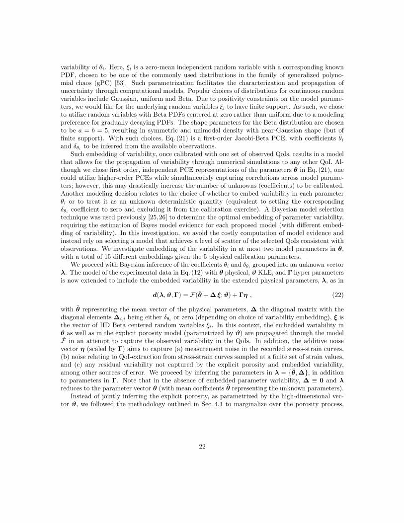
Such embedding of variability, once calibrated with one set of observed QoIs, results in a modelthat allows for the propagation of variability through numerical simulations to any other QoI. Al-though we chose first order, independent PCE representations of the parameters θ in Eq. (21), onecould utilize higher-order PCEs while simultaneously capturing correlations across model parame-ters; however, this may drastically increase the number of unknowns (coefficients) to be calibrated.Another modeling decision relates to the choice of whether to embed variability in each parameterθi or to treat it as an unknown deterministic quantity (equivalent to setting the correspondingδθi coefficient to zero and excluding it from the calibration exercise). A Bayesian model selectiontechnique was used previously [25,26] to determine the optimal embedding of parameter variability,requiring the estimation of Bayes model evidence for each proposed model (with different embed-ding of variability). In this investigation, we avoid the costly computation of model evidence andinstead rely on selecting a model that achieves a level of scatter of the selected QoIs consistent withobservations. We investigate embedding of the variability in at most two model parameters in θ,with a total of 15 different embeddings given the 5 physical calibration parameters.

We proceed with Bayesian inference of the coefficients θi and δθi grouped into an unknown vectorλ. The model of the experimental data in Eq. (12) with θ physical, ϑ KLE, and Γ hyper parametersis now extended to include the embedded variability in the extended physical parameters, λ, as in

d(λ,ϑ,Γ) = F(θ + ∆ ξ;ϑ) + Γη , (22)

with θ representing the mean vector of the physical parameters, ∆ the diagonal matrix with thediagonal elements ∆i,i being either δθi or zero (depending on choice of variability embedding), ξ isthe vector of IID Beta centered random variables ξi. In this context, the embedded variability inθ as well as in the explicit porosity model (parametrized by ϑ) are propagated through the modelF in an attempt to capture the observed variability in the QoIs. In addition, the additive noisevector η (scaled by Γ) aims to capture (a) measurement noise in the recorded stress-strain curves,(b) noise relating to QoI-extraction from stress-strain curves sampled at a finite set of strain values,and (c) any residual variability not captured by the explicit porosity and embedded variability,among other sources of error. We proceed by inferring the parameters in λ = θ,∆, in additionto parameters in Γ. Note that in the absence of embedded parameter variability, ∆ ≡ 0 and λreduces to the parameter vector θ (with mean coefficients θ representing the unknown parameters).

Instead of jointly inferring the explicit porosity, as parametrized by the high-dimensional vec-tor ϑ, we followed the methodology outlined in Sec. 4.1 to marginalize over the porosity process,

22

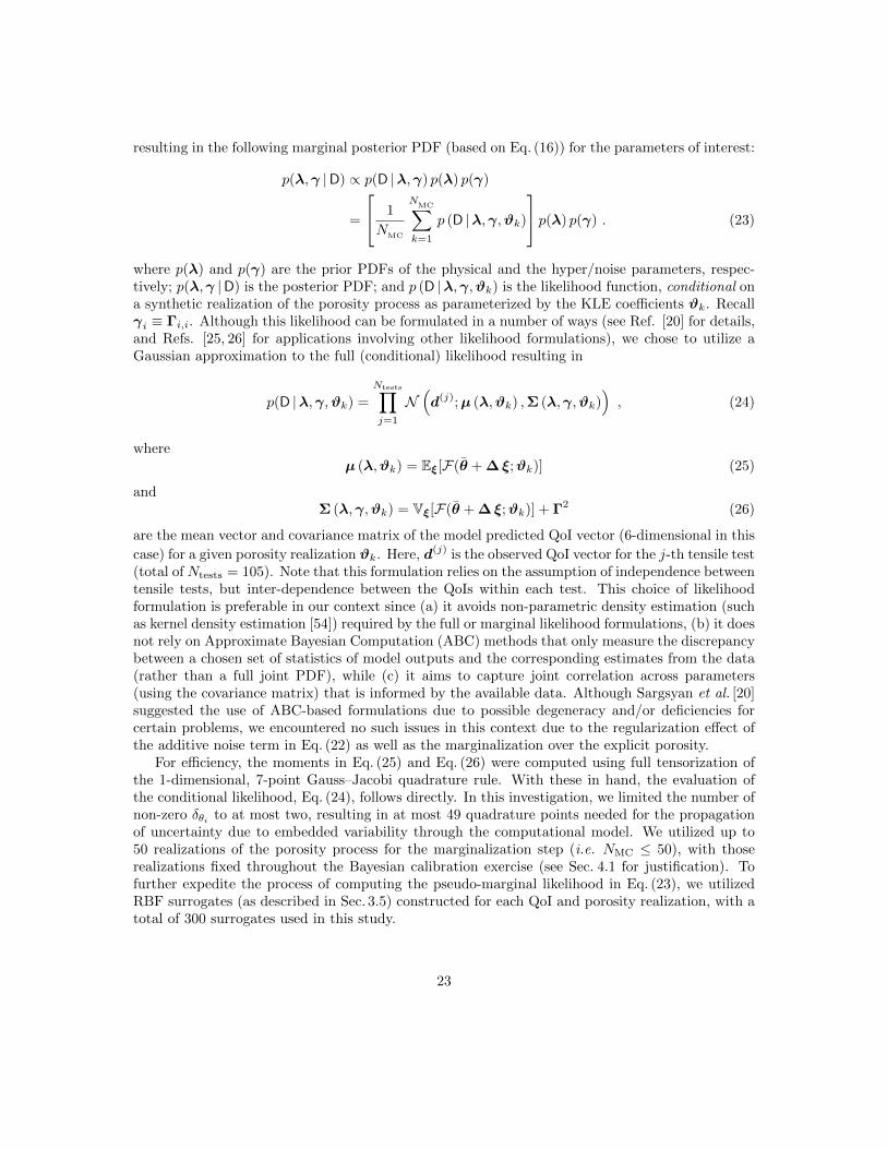
resulting in the following marginal posterior PDF (based on Eq. (16)) for the parameters of interest:

p(λ,γ |D) ∝ p(D |λ,γ) p(λ) p(γ)

=

1

NMC

NMC∑k=1

p (D |λ,γ,ϑk)

p(λ) p(γ) . (23)

where p(λ) and p(γ) are the prior PDFs of the physical and the hyper/noise parameters, respec-tively; p(λ,γ |D) is the posterior PDF; and p (D |λ,γ,ϑk) is the likelihood function, conditional ona synthetic realization of the porosity process as parameterized by the KLE coefficients ϑk. Recallγi ≡ Γi,i. Although this likelihood can be formulated in a number of ways (see Ref. [20] for details,and Refs. [25, 26] for applications involving other likelihood formulations), we chose to utilize aGaussian approximation to the full (conditional) likelihood resulting in

p(D |λ,γ,ϑk) =

Ntests∏j=1

N(d(j);µ (λ,ϑk) ,Σ (λ,γ,ϑk)

), (24)

whereµ (λ,ϑk) = Eξ[F(θ + ∆ ξ;ϑk)] (25)

andΣ (λ,γ,ϑk) = Vξ[F(θ + ∆ ξ;ϑk)] + Γ2 (26)

are the mean vector and covariance matrix of the model predicted QoI vector (6-dimensional in this

case) for a given porosity realization ϑk. Here, d(j) is the observed QoI vector for the j-th tensile test(total of Ntests = 105). Note that this formulation relies on the assumption of independence betweentensile tests, but inter-dependence between the QoIs within each test. This choice of likelihoodformulation is preferable in our context since (a) it avoids non-parametric density estimation (suchas kernel density estimation [54]) required by the full or marginal likelihood formulations, (b) it doesnot rely on Approximate Bayesian Computation (ABC) methods that only measure the discrepancybetween a chosen set of statistics of model outputs and the corresponding estimates from the data(rather than a full joint PDF), while (c) it aims to capture joint correlation across parameters(using the covariance matrix) that is informed by the available data. Although Sargsyan et al. [20]suggested the use of ABC-based formulations due to possible degeneracy and/or deficiencies forcertain problems, we encountered no such issues in this context due to the regularization effect ofthe additive noise term in Eq. (22) as well as the marginalization over the explicit porosity.

For efficiency, the moments in Eq. (25) and Eq. (26) were computed using full tensorization ofthe 1-dimensional, 7-point Gauss–Jacobi quadrature rule. With these in hand, the evaluation ofthe conditional likelihood, Eq. (24), follows directly. In this investigation, we limited the number ofnon-zero δθi to at most two, resulting in at most 49 quadrature points needed for the propagationof uncertainty due to embedded variability through the computational model. We utilized up to50 realizations of the porosity process for the marginalization step (i.e. NMC ≤ 50), with thoserealizations fixed throughout the Bayesian calibration exercise (see Sec. 4.1 for justification). Tofurther expedite the process of computing the pseudo-marginal likelihood in Eq. (23), we utilizedRBF surrogates (as described in Sec. 3.5) constructed for each QoI and porosity realization, with atotal of 300 surrogates used in this study.

23

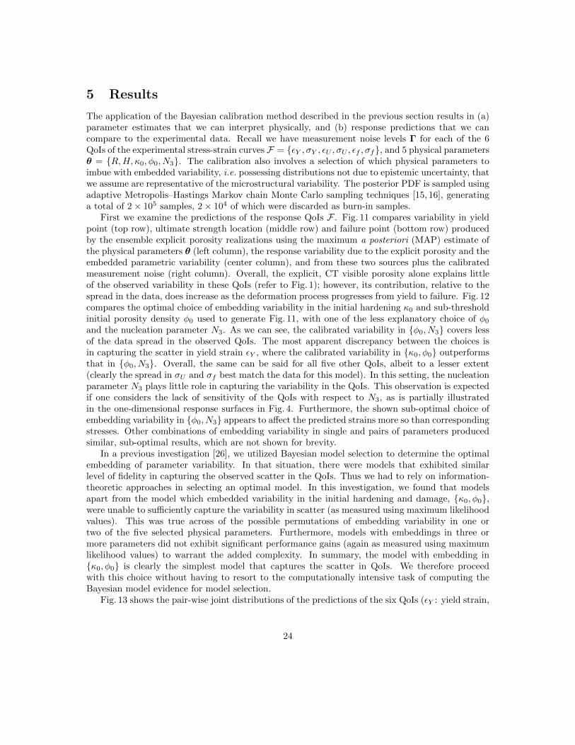
5 Results

The application of the Bayesian calibration method described in the previous section results in (a)parameter estimates that we can interpret physically, and (b) response predictions that we cancompare to the experimental data. Recall we have measurement noise levels Γ for each of the 6QoIs of the experimental stress-strain curves F = εY , σY , εU , σU , εf , σf, and 5 physical parametersθ = R,H, κ0, φ0, N3. The calibration also involves a selection of which physical parameters toimbue with embedded variability, i.e. possessing distributions not due to epistemic uncertainty, thatwe assume are representative of the microstructural variability. The posterior PDF is sampled usingadaptive Metropolis–Hastings Markov chain Monte Carlo sampling techniques [15, 16], generatinga total of 2× 105 samples, 2× 104 of which were discarded as burn-in samples.

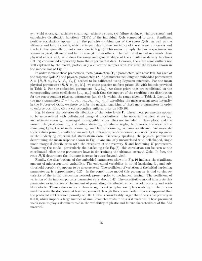
First we examine the predictions of the response QoIs F . Fig. 11 compares variability in yieldpoint (top row), ultimate strength location (middle row) and failure point (bottom row) producedby the ensemble explicit porosity realizations using the maximum a posteriori (MAP) estimate ofthe physical parameters θ (left column), the response variability due to the explicit porosity and theembedded parametric variability (center column), and from these two sources plus the calibratedmeasurement noise (right column). Overall, the explicit, CT visible porosity alone explains littleof the observed variability in these QoIs (refer to Fig. 1); however, its contribution, relative to thespread in the data, does increase as the deformation process progresses from yield to failure. Fig. 12compares the optimal choice of embedding variability in the initial hardening κ0 and sub-thresholdinitial porosity density φ0 used to generate Fig. 11, with one of the less explanatory choice of φ0

and the nucleation parameter N3. As we can see, the calibrated variability in φ0, N3 covers lessof the data spread in the observed QoIs. The most apparent discrepancy between the choices isin capturing the scatter in yield strain εY , where the calibrated variability in κ0, φ0 outperformsthat in φ0, N3. Overall, the same can be said for all five other QoIs, albeit to a lesser extent(clearly the spread in σU and σf best match the data for this model). In this setting, the nucleationparameter N3 plays little role in capturing the variability in the QoIs. This observation is expectedif one considers the lack of sensitivity of the QoIs with respect to N3, as is partially illustratedin the one-dimensional response surfaces in Fig. 4. Furthermore, the shown sub-optimal choice ofembedding variability in φ0, N3 appears to affect the predicted strains more so than correspondingstresses. Other combinations of embedding variability in single and pairs of parameters producedsimilar, sub-optimal results, which are not shown for brevity.

In a previous investigation [26], we utilized Bayesian model selection to determine the optimalembedding of parameter variability. In that situation, there were models that exhibited similarlevel of fidelity in capturing the observed scatter in the QoIs. Thus we had to rely on information-theoretic approaches in selecting an optimal model. In this investigation, we found that modelsapart from the model which embedded variability in the initial hardening and damage, κ0, φ0,were unable to sufficiently capture the variability in scatter (as measured using maximum likelihoodvalues). This was true across of the possible permutations of embedding variability in one ortwo of the five selected physical parameters. Furthermore, models with embeddings in three ormore parameters did not exhibit significant performance gains (again as measured using maximumlikelihood values) to warrant the added complexity. In summary, the model with embedding inκ0, φ0 is clearly the simplest model that captures the scatter in QoIs. We therefore proceedwith this choice without having to resort to the computationally intensive task of computing theBayesian model evidence for model selection.

Fig. 13 shows the pair-wise joint distributions of the predictions of the six QoIs (εY : yield strain,

24

σY : yield stress, εU : ultimate strain, σU : ultimate stress, εf : failure strain, σf : failure stress) andcumulative distribution functions (CDFs) of the individual QoIs compared to data. Significantpositive correlations appear in all the pairwise combinations of the stress QoIs, as well as theultimate and failure strains, which is in part due to due continuity of the stress-strain curves andthe fact they generally do not cross (refer to Fig. 1). This seems to imply that some specimens areweaker in yield, ultimate and failure strength than others. The calibrated model represents thesephysical effects well, as it does the range and general shape of the cumulative density functions(CDFs) constructed empirically from the experimental data. However, there are some outliers notwell captured by the model, particularly a cluster of samples with low ultimate stresses shown inthe middle row of Fig. 13.

In order to make these predictions, meta parameters (Γ, 6 parameters, one noise level for each ofthe response QoIs F) and physical parameters (λ, 7 parameters including the embedded parameters:λ = R, H, κ0, φ0, N3, δκ0 , δφ0) needed to be calibrated using Bayesian inference. For the meanphysical parameters R, H, κ0, φ0, N3, we chose positive uniform priors [55] with bounds providedin Table 2. For the embedded parameters δκ0

, δφ0, we chose priors that are conditional on the

corresponding mean coefficients µκ0, µφ0 such that the support of the resulting beta distribution

for the corresponding physical parameters κ0, φ0 is within the range given in Table 2. Lastly, forthe meta parameters Γ = γεY , γσY

, γεU , γσU, γεf , γσf

describing the measurement noise intensityin the 6 observed QoIs, we chose to infer the natural logarithm of those meta parameters in orderto enforce positivity, with a corresponding uniform prior on [-20,20].

Fig. 14 shows the posterior distributions of the noise levels Γ. These meta parameters appearto be uncorrelated with bell-shaped marginal distributions. The noise in the yield stress γσY

and ultimate stress γσUconverged to negligible values (thus not included in these plots) and the

noise in the yield strain γεY and failure stress γσfare almost negligible; however, the noise in the

remaining QoIs, the ultimate strain γεU and failure strain γεf remains significant. We associatethese values primarily with the inexact QoI extraction, since measurement noise is not apparentin the underlying experimental stress-strain data. Generally speaking, the physical parametersdetermining the mean response shown in Fig. 15 are similarly uncorrelated with bell-shaped, singlemode marginal distributions with the exception of the recovery R and hardening H parameters.Examining the model, particularly the hardening rule Eq. (3), this correlation can be seen as thecoordinated effect these parameters have in determining the ultimate strength QoIs. In fact, theratio H/R determines the ultimate increase in stress beyond yield.

Finally, the distributions of the embedded parameters shown in Fig. 16 indicate the significantamount of microstructural variability. The embedded variability in initial hardening δκ0 and sub-threshold porosity δφ0 appear to be uncorrelated. The coefficient of variation of the initial hardeningparameter κ0 is approximately 0.25. In the constitutive model this parameter is tied to charac-teristics of the initial dislocation network present prior to mechanical testing. The coefficient ofvariation of the implicit porosity parameter φ0 is about 0.42. The constitutive model interprets thisparameter as indicative of the amount of preexisting, distributed, sub-threshold porosity and void-like defects. These values indicate there is significant sample-to-sample variability in the processused to create the dogbones, at least as perceived through the chosen model. It is also apparent thatthe predicted subthreshold porosity of 0.09 ± 0.04 is considerably larger than the visible porosity ≈0.008, which implies a large number of small diameter voids in this AM material. These presumedvoids seem to play a dominant role in the variability of plastic and failure characteristics of the AMmaterial.

25

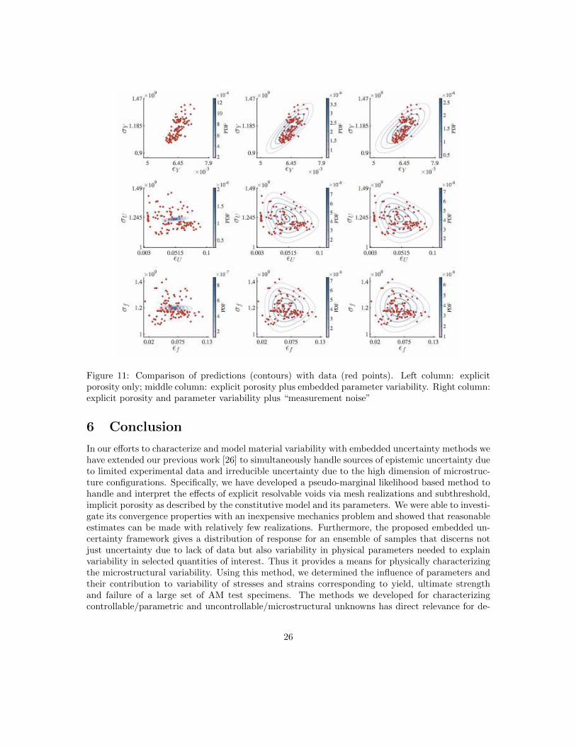
Figure 11: Comparison of predictions (contours) with data (red points). Left column: explicitporosity only; middle column: explicit porosity plus embedded parameter variability. Right column:explicit porosity and parameter variability plus “measurement noise”

6 Conclusion

In our efforts to characterize and model material variability with embedded uncertainty methods wehave extended our previous work [26] to simultaneously handle sources of epistemic uncertainty dueto limited experimental data and irreducible uncertainty due to the high dimension of microstruc-ture configurations. Specifically, we have developed a pseudo-marginal likelihood based method tohandle and interpret the effects of explicit resolvable voids via mesh realizations and subthreshold,implicit porosity as described by the constitutive model and its parameters. We were able to investi-gate its convergence properties with an inexpensive mechanics problem and showed that reasonableestimates can be made with relatively few realizations. Furthermore, the proposed embedded un-certainty framework gives a distribution of response for an ensemble of samples that discerns notjust uncertainty due to lack of data but also variability in physical parameters needed to explainvariability in selected quantities of interest. Thus it provides a means for physically characterizingthe microstructural variability. Using this method, we determined the influence of parameters andtheir contribution to variability of stresses and strains corresponding to yield, ultimate strengthand failure of a large set of AM test specimens. The methods we developed for characterizingcontrollable/parametric and uncontrollable/microstructural unknowns has direct relevance for de-

26

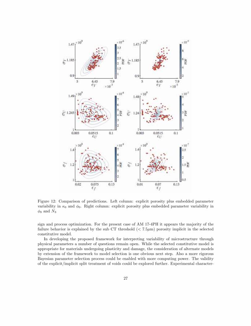
Figure 12: Comparison of predictions. Left column: explicit porosity plus embedded parametervariability in κ0 and φ0. Right column: explicit porosity plus embedded parameter variability inφ0 and N3

sign and process optimization. For the present case of AM 17-4PH it appears the majority of thefailure behavior is explained by the sub CT threshold (< 7.5µm) porosity implicit in the selectedconstitutive model.

In developing the proposed framework for interpreting variability of microstructure throughphysical parameters a number of questions remain open. While the selected constitutive model isappropriate for materials undergoing plasticity and damage, the consideration of alternate modelsby extension of the framework to model selection is one obvious next step. Also a more rigorousBayesian parameter selection process could be enabled with more computing power. The validityof the explicit/implicit split treatment of voids could be explored further. Experimental character-

27

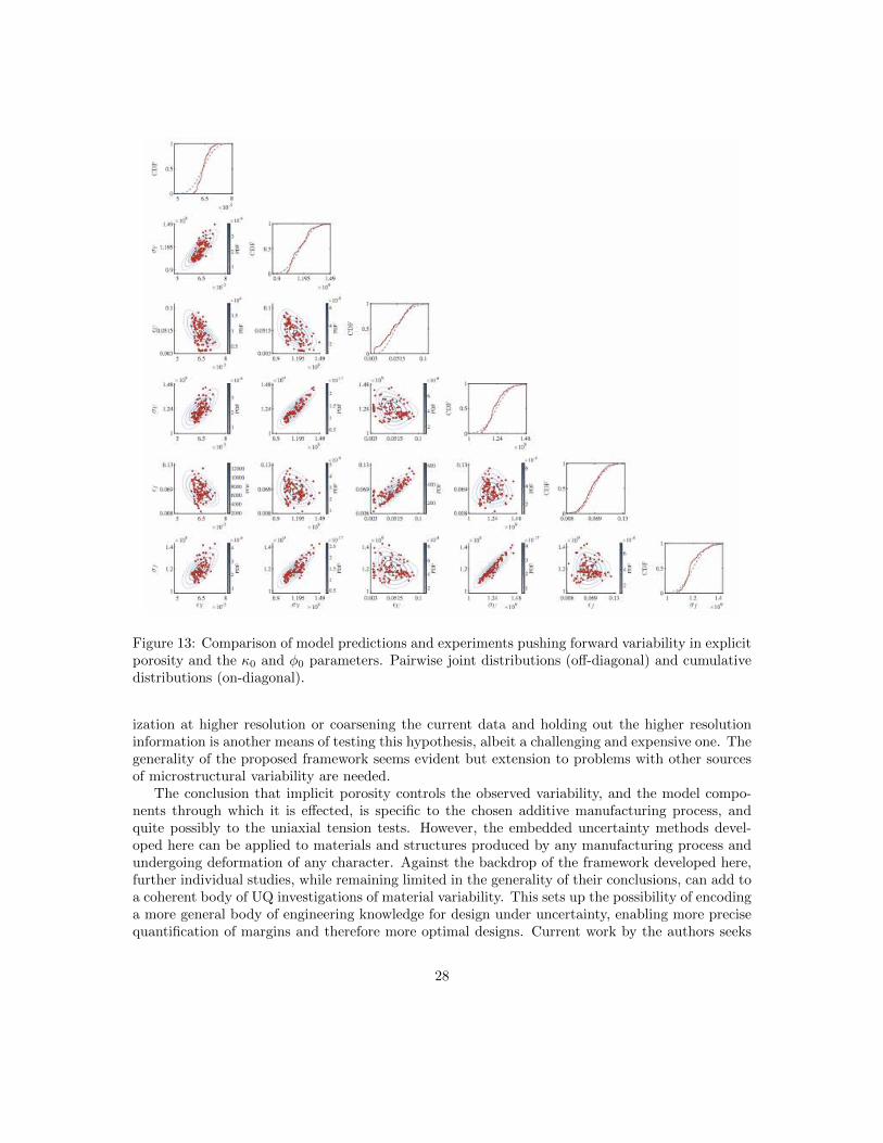
Figure 13: Comparison of model predictions and experiments pushing forward variability in explicitporosity and the κ0 and φ0 parameters. Pairwise joint distributions (off-diagonal) and cumulativedistributions (on-diagonal).

ization at higher resolution or coarsening the current data and holding out the higher resolutioninformation is another means of testing this hypothesis, albeit a challenging and expensive one. Thegenerality of the proposed framework seems evident but extension to problems with other sourcesof microstructural variability are needed.

The conclusion that implicit porosity controls the observed variability, and the model compo-nents through which it is effected, is specific to the chosen additive manufacturing process, andquite possibly to the uniaxial tension tests. However, the embedded uncertainty methods devel-oped here can be applied to materials and structures produced by any manufacturing process andundergoing deformation of any character. Against the backdrop of the framework developed here,further individual studies, while remaining limited in the generality of their conclusions, can add toa coherent body of UQ investigations of material variability. This sets up the possibility of encodinga more general body of engineering knowledge for design under uncertainty, enabling more precisequantification of margins and therefore more optimal designs. Current work by the authors seeks

28

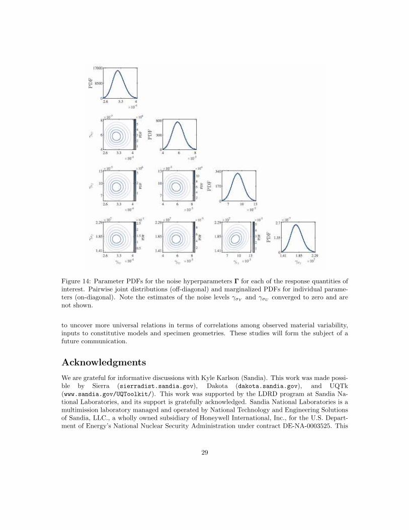
Figure 14: Parameter PDFs for the noise hyperparameters Γ for each of the response quantities ofinterest. Pairwise joint distributions (off-diagonal) and marginalized PDFs for individual parame-ters (on-diagonal). Note the estimates of the noise levels γσY

and γσUconverged to zero and are

not shown.

to uncover more universal relations in terms of correlations among observed material variability,inputs to constitutive models and specimen geometries. These studies will form the subject of afuture communication.

Acknowledgments

We are grateful for informative discussions with Kyle Karlson (Sandia). This work was made possi-ble by Sierra (sierradist.sandia.gov), Dakota (dakota.sandia.gov), and UQTk(www.sandia.gov/UQToolkit/). This work was supported by the LDRD program at Sandia Na-tional Laboratories, and its support is gratefully acknowledged. Sandia National Laboratories is amultimission laboratory managed and operated by National Technology and Engineering Solutionsof Sandia, LLC., a wholly owned subsidiary of Honeywell International, Inc., for the U.S. Depart-ment of Energy’s National Nuclear Security Administration under contract DE-NA-0003525. This

29

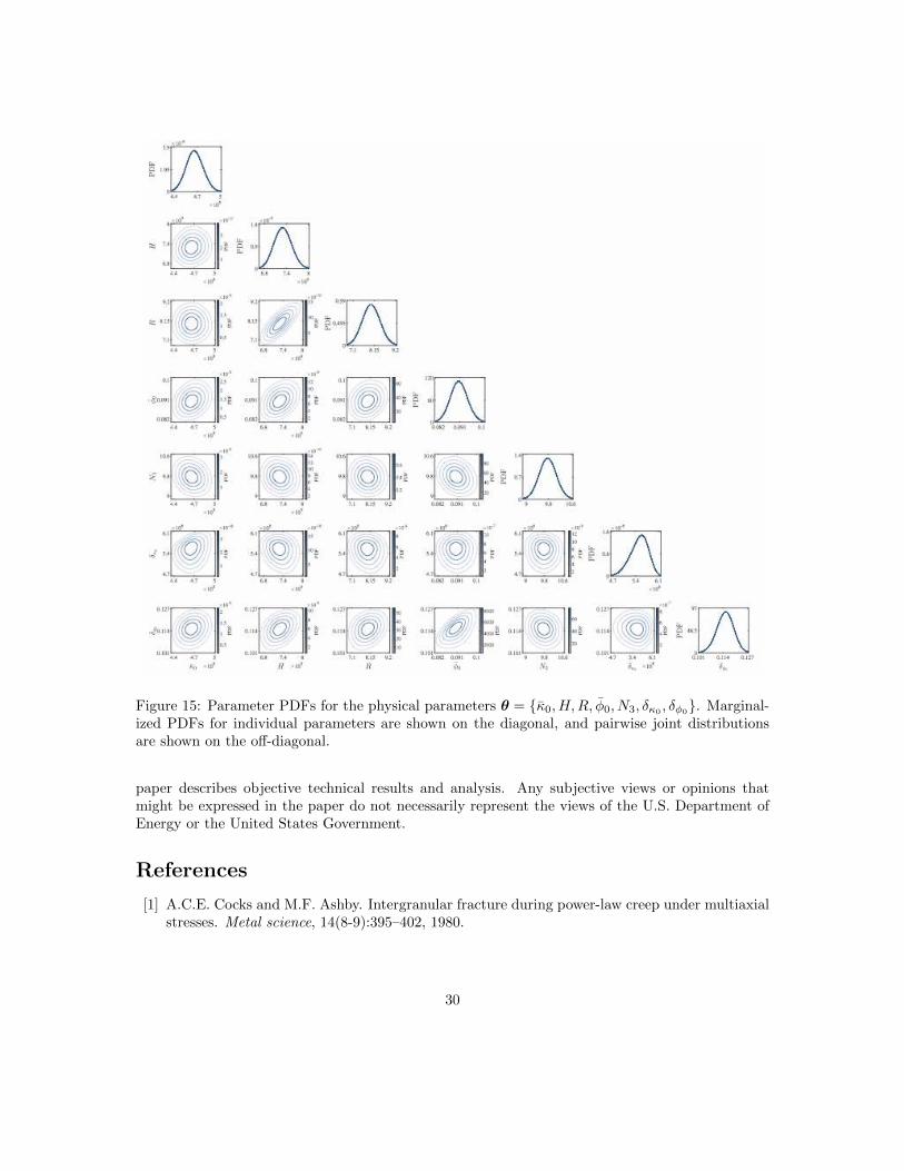
Figure 15: Parameter PDFs for the physical parameters θ = κ0, H,R, φ0, N3, δκ0, δφ0. Marginal-

ized PDFs for individual parameters are shown on the diagonal, and pairwise joint distributionsare shown on the off-diagonal.

paper describes objective technical results and analysis. Any subjective views or opinions thatmight be expressed in the paper do not necessarily represent the views of the U.S. Department ofEnergy or the United States Government.

References

[1] A.C.E. Cocks and M.F. Ashby. Intergranular fracture during power-law creep under multiaxialstresses. Metal science, 14(8-9):395–402, 1980.

30

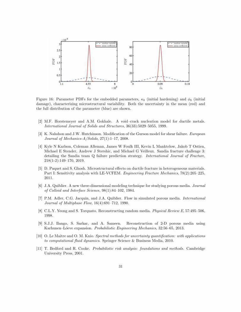
Figure 16: Parameter PDFs for the embedded parameters, κ0 (initial hardening) and φ0 (initialdamage), characterizing microstructural variability. Both the uncertainty in the mean (red) andthe full distribution of the parameter (blue) are shown.

[2] M.F. Horstemeyer and A.M. Gokhale. A void–crack nucleation model for ductile metals.International Journal of Solids and Structures, 36(33):5029–5055, 1999.

[3] K. Nahshon and J.W. Hutchinson. Modification of the Gurson model for shear failure. EuropeanJournal of Mechanics-A/Solids, 27(1):1–17, 2008.

[4] Kyle N Karlson, Coleman Alleman, James W Foulk III, Kevin L Manktelow, Jakob T Ostien,Michael E Stender, Andrew J Stershic, and Michael G Veilleux. Sandia fracture challenge 3:detailing the Sandia team Q failure prediction strategy. International Journal of Fracture,218(1-2):149–170, 2019.

[5] D. Paquet and S. Ghosh. Microstructural effects on ductile fracture in heterogeneous materials.Part I: Sensitivity analysis with LE-VCFEM. Engineering Fracture Mechanics, 78(2):205–225,2011.

[6] J.A. Quiblier. A new three-dimensional modeling technique for studying porous media. Journalof Colloid and Interface Science, 98(1):84–102, 1984.

[7] P.M. Adler, C.G. Jacquin, and J.A. Quiblier. Flow in simulated porous media. InternationalJournal of Multiphase Flow, 16(4):691–712, 1990.

[8] C.L.Y. Yeong and S. Torquato. Reconstructing random media. Physical Review E, 57:495–506,1998.

[9] S.J.J. Ilango, S. Sarkar, and A. Sameen. Reconstruction of 2-D porous media usingKarhunen–Loeve expansion. Probabilistic Engineering Mechanics, 32:56–65, 2013.

[10] O. Le Maıtre and O. M. Knio. Spectral methods for uncertainty quantification: with applicationsto computational fluid dynamics. Springer Science & Business Media, 2010.

[11] T. Bedford and R. Cooke. Probabilistic risk analysis: foundations and methods. CambridgeUniversity Press, 2001.

31

[12] R.L. Winkler. Uncertainty in probabilistic risk assessment. Reliability Engineering & SystemSafety, 54(2):127–132, 1996.

[13] C. Andrieu and G.O. Roberts. The pseudo-marginal approach for efficient Monte Carlo com-putations. Annals of Statistics, 37(2):697–725, 2009.

[14] P.D. O’Neill, D.J. Balding, N.G. Becker, M. Eerola, and D. Mollison. Analyses of infectiousdisease data from household outbreaks by Markov chain Monte Carlo methods. Journal of theRoyal Statistical Society: Series C (Applied Statistics), 49(4):517–542, 2000.

[15] D. Gamerman and H.F. Lopes. Markov chain Monte Carlo: stochastic simulation for Bayesianinference. CRC Press, 2006.

[16] B.A. Berg and A. Billoire. Markov chain Monte Carlo simulations. Wiley Online Library,2008.

[17] Marc C Kennedy and Anthony O’Hagan. Bayesian calibration of computer models. Journalof the Royal Statistical Society: Series B (Statistical Methodology), 63(3):425–464, 2001.

[18] C. Soize. A nonparametric model of random uncertainties for reduced matrix models in struc-tural dynamics. Probabilistic Engineering Mechanics, 15(3):277–294, 2000.

[19] M. Strong and J. Oakley. When is a model good enough? Deriving the expected value ofmodel improvement via specifying internal model discrepancies. SIAM/ASA J UncertaintyQuantification, 2:106–125, 2014.

[20] K. Sargsyan, H.N. Najm, and R. Ghanem. On the statistical calibration of physical models.International Journal of Chemical Kinetics, 47(4):246–276, 2015.

[21] Yanyan He and Dongbin Xiu. Numerical strategy for model correction using physical con-straints. Journal of Computational Physics, 313:617–634, 2016.

[22] Pascal Pernot and Fabien Cailliez. A critical review of statistical calibration/prediction modelshandling data inconsistency and model inadequacy. AIChE Journal, 63(10):4642–4665, 2017.

[23] Souleymane Zio, Henrique F. da Costa, Gabriel M. Guerra, Paulo L.B. Paraizo, Jose J. Camata,Renato N. Elias, Alvaro L.G.A. Coutinho, and Fernando A. Rochinha. Bayesian assessment ofuncertainty in viscosity closure models for turbidity currents computations. Computer Methodsin Applied Mechanics and Engineering, 342:653 – 673, 2018.

[24] Rebecca E. Morrison, Todd A. Oliver, and Robert D. Moser. Representing model inadequacy:A stochastic operator approach. SIAM/ASA J Uncertainty Quantification, 6(2):457–496, 2018.

[25] L. Hakim, G. Lacaze, M. Khalil, K. Sargsyan, H. Najm, and J. Oefelein. Probabilistic parameterestimation in a 2-step chemical kinetics model for n-dodecane jet autoignition. CombustionTheory and Modelling, 22(3), 2018.

[26] F. Rizzi, M. Khalil, R.E. Jones, J.A. Templeton, J.T. Ostien, and B.L. Boyce. Bayesianmodeling of inconsistent plastic response due to material variability. Computer Methods inApplied Mechanics and Engineering, 353:183–200, 2019.

32

[27] J.M. Emery, R.V. Field, J.W. Foulk, K.N. Karlson, and M.D. Grigoriu. Predicting laser weldreliability with stochastic reduced-order models. International Journal for Numerical Methodsin Engineering, 103(12):914–936, 2015.

[28] R.V. Field, M.D. Grigoriu, and J.M. Emery. On the efficacy of stochastic collocation, stochasticGalerkin, and stochastic reduced order models for solving stochastic problems. ProbabilisticEngineering Mechanics, 41:60–72, 2015.

[29] H. Rappel, L.A.A. Beex, L. Noels, and S.P.A. Bordas. Identifying elastoplastic parameterswith bayes’ theorem considering output error, input error and model uncertainty. ProbabilisticEngineering Mechanics, 2018.

[30] A. Kucerova and H.G. Matthies. Uncertainty updating in the description of heterogeneousmaterials. Technische Mechanik, 30(1-3):211–226, 2010.

[31] B.L. Boyce, B.C. Salzbrenner, J.M. Rodelas, L.P. Swiler, J.D. Madison, B.H. Jared, and Y.-L.Shen. Extreme-value statistics reveal rare failure-critical defects in additive manufacturing.Advanced Engineering Materials, 2017.

[32] N.M. Heckman et al. Micro-CT observation of void network evolution in additively manufac-tured 316L under tensile loading. in preparation, 2019.

[33] D.J. Bammann, M.L. Chiesa, and G.C. Johnson. Modeling large deformation and failure inmanufacturing processes. Theoretical and Applied Mechanics, 9:359–376, 1996.

[34] A.A. Brown and D.J. Bammann. Validation of a model for static and dynamic recrystallizationin metals. International Journal of Plasticity, 32:17–35, 2012.

[35] K.N. Karlson, J.W. Foulk, A.A. Brown, and M.G. Veilleux. Sandia fracture challenge 2: SandiaCalifornia’s modeling approach. International Journal of Fracture, 198(1-2):179–195, 2016.

[36] P. Guttorp and P.D. Sampson. Methods for estimating heterogeneous spatial covariance func-tions with environmental applications. In Environmental Statistics, volume 12 of Handbook ofStatistics, pages 661–689. Elsevier, 1994.

[37] B.D. Ripley. Spatial Statistics. John Wiley, 1981.

[38] N. Cressie. Statistics for Spatial Data. John Wiley, 1991.

[39] N. Wiener. The Homogeneous Chaos. American Journal of Mathematics, 60:897–936, 1938.

[40] R.G. Ghanem and P.D. Spanos. Stochastic Finite Elements: A Spectral Approach. SpringerVerlag, New York, 1991.

[41] R.L. Hardy. Multiquadric equations of topography and other irregular surfaces. Journal ofGeophysical Research (1896-1977), 76(8):1905–1915, 1971.

[42] N. Dyn, D. Levin, and S. Rippa. Numerical procedures for surface fitting of scattered data byradial functions. SIAM Journal on Scientific and Statistical Computing, 7(2):639–659, 1986.

[43] M.J.D. Powell. Radial basis functions for multivariable interpolation: A review. In J.C. Masonand M.G. Cox, editors, Algorithms for Approximation, pages 143–167. Clarendon Press, NewYork, NY, USA, 1987.

33

[44] R. Jin, W. Chen, and T.W. Simpson. Comparative studies of metamodelling techniques undermultiple modelling criteria. Structural and Multidisciplinary Optimization, 23(1):1–13, 2001.

[45] H.-M. Gutmann. A radial basis function method for global optimization. Journal of GlobalOptimization, 19(3):201–227, 2001.

[46] G.E. Fasshauer and J.G. Zhang. On choosing optimal shape parameters for RBF approxima-tion. Numerical Algorithms, 45(1):345–368, 2007.

[47] R. Franke. Scattered data interpolation: Tests of some method. Mathematics of Computation,38(157):181–200, 1982.

[48] H. Wendland and C. Rieger. Approximate interpolation with applications to selecting smooth-ing parameters. Numerische Mathematik, 101(4):729–748, 2005.

[49] S. Arlot and A. Celisse. A survey of cross-validation procedures for model selection. StatisticsSurveys, 4:40–79, 2010.

[50] J. Sacks, S.B. Schiller, and W.J. Welch. Designs for computer experiments. Technometrics,31(1):41–47, 1989.

[51] X. Wei, Y.-Z. Wu, and L.-P. Chen. A new sequential optimal sampling method for radial basisfunctions. Applied Mathematics and Computation, 218(19):9635 – 9646, 2012.

[52] R.W. Clough and J. Penzien. Dynamics of structures. McGraw-Hill, 1975.

[53] D. Xiu and G.E. Karniadakis. The Wiener-Askey polynomial chaos for stochastic differentialequations. SIAM Journal on Scientific Computing, 24(2):619–644, 2002.

[54] B.W. Silverman. Density Estimation for Statistics and Data Analysis. Chapman & Hall, 1986.

[55] W.M. Bolstad and J.M. Curran. Introduction to Bayesian statistics. John Wiley & Sons, 2016.

A Karhunen-Loeve Representation of the Porosity Process

Given the experimental mean porosity ϕ and spatial correlation of the observable voids, Rϕϕ(r), weconstruct a Karhunen-Loeve (KL) representation of the porosity process follow the methodologyproposed by Ilango et al. [9]. Specifically, we model the random porosity of the test specimens as abinary random process given by

ϕ(x) =

1 , x ∈ void region0 , otherwise

(A.1)

with mean porosity of ϕ (i.e. P(ϕ = 1) = ϕ) and the variance of this process is ϕ(1 − ϕ). Weassume that the process is homogeneous and possesses an isotropic two-point correlation functiongiven by

Rϕϕ (x1,x2) = E [ϕ (x1)ϕ (x2)] . (A.2)

Alternatively, we can model the normalized (zero-mean and unit-variance) process using thelinear transform:

Z =ϕ− ϕ√ϕ(1− ϕ)

. (A.3)

34

The binary random process Z(x) is constructed through an intermediate zero-mean, unit-varianceGaussian process Y(x) modeled using KLE. This involves transforming Y (a continuous process)to Z (a binary process) using the mapping:

z = z (y) =

ϕ−1√ϕ(1−ϕ)

, y < y∗

ϕ√ϕ(1−ϕ)

, otherwise(A.4)

with the threshold y∗ satisfying the identity [9]:

1√2π

∫ y∗

−∞e−t

2/2 dt = ϕ . (A.5)

chosen to preserve the mean porosity ϕ.The correlation functions of processes Z and Y are related through the following identity

RZZ(x1,x2) = E [Z(x1)Z(x2)]

=

∫Z(x1)Z(x2) pZZ (Z(x1),Z(x2)) dZ(x1)dZ(x2)

=

∫z(Y(x1))z(Y(x2)) pYY (Y(x1),Y(x2)) dY(x1)dY(x2)

=

∫z(y1)z(y2) pYY (y1, y2) dy1dy2 (A.6)

with y1 = Y(x1) and y1 = Y(x2) used to simplify the exposition. Since Y is assumed to be aGaussian random process with unknown correlation function RYY(x1,x2), we can write the jointPDF, pYY (Y(x1),Y(x2)), in terms of RYY as

pYY (Y(x1),Y(x2)) =e−((y21−2RYY(x1,x2)y1y2+y22)/(2(1−R2

YY(x1,x2))))

2π√

1− R2YY (x1,x2)

(A.7)

Eq. (A.6) relates the known correlation function for the binary random process modeling therandom porosity, RZZ (x1,x2), to that of the intermediate Gaussian random process RYY (x1,x2).Expanding the joint PDF pYY (Y(x1),Y(x2)) in terms of Hermite polynomials as in [9]

pYY (y1, y2) =

∞∑m=0

RmYYm!

Hm (y1)Hm (y2) %(y1)%(y2) (A.8)

with Hm denoting the Hermite polynomial of order m and % the standard Gaussian PDF. Thisexpansion allows us to rewrite Eq. (A.6) as [9]

RZZ (x1,x2) =

∞∑m=0

K2mRmYY (A.9)

with

Km =1√m!

∫z (y)Hm (y)φ (y) dy . (A.10)

35

where we approximate Km with Gauss-Hermite quadrature. For this application, Eq. (A.9) istruncated to 30 terms (chosen via a convergence study with results not included for brevity) andRYY is solved for numerically using a root-finding algorithm over different values of RZZ .

This procedure provides a mechanism to transform the two-point correlation of the normalizedbinary random process, Z, modeling the random porosity (obtained from observations) to that of theintermediate Gaussian random process, Y. This intermediate Gaussian process was approximatedby KLE as

Y(x) ≈L∑j=1

ϑjζj(x) (A.11)

where ζj =√λjfj(x), and λj , fjLj=1 are the first L-th eigenvalues and eigenfunctions of the

correlation function RYY and the number of terms L is optimally selected to capture 99.9% of theenergy (variance) of the process. ϑjLj=1 are independent standard Gaussian random variables.For certain correlation functions, the eigenfunctions and eigenvalues are available in closed-form orsemi-analytically (e.g. as numerical solutions to root-finding problems). In general, however, oneresorts to spatial discretization of the random process on the domain of interest that effectivelymaps it to a random vector (with the correlation function mapped to a covariance matrix) whichcan subsequently undergo a spectral decomposition to obtain the eigenvalue/eigenvector pairs. SeeRef. [10] for details.

36