1

Predicting retail website anomalies using Twitter data

Derek Farren

dfarren@walmartlabs.com

December 14th, 2012

Abstract – Anomalies in website performance are very common. Most of the time they are short and only affect a small portion of the users. However, in e-commerce an anomaly is very expensive. Just one minute with an underperforming site means a big loss for a big e-commerce retailer. This project presents a way to detect those anomalies in real time and to predict them with up to one hour in advance. Index Terms – Machine Learning, Anomaly prediction, e-commerce, Web performance.

INTRODUCTION

E-commerce web site operations are heavily transactional and prone to small, short time failures. Most of the time these anomalies are small, and as such, they are not caught by the retailer web operations. However, the customers do perceive these anomalies. In this project I propose a model to predict website anomalies.

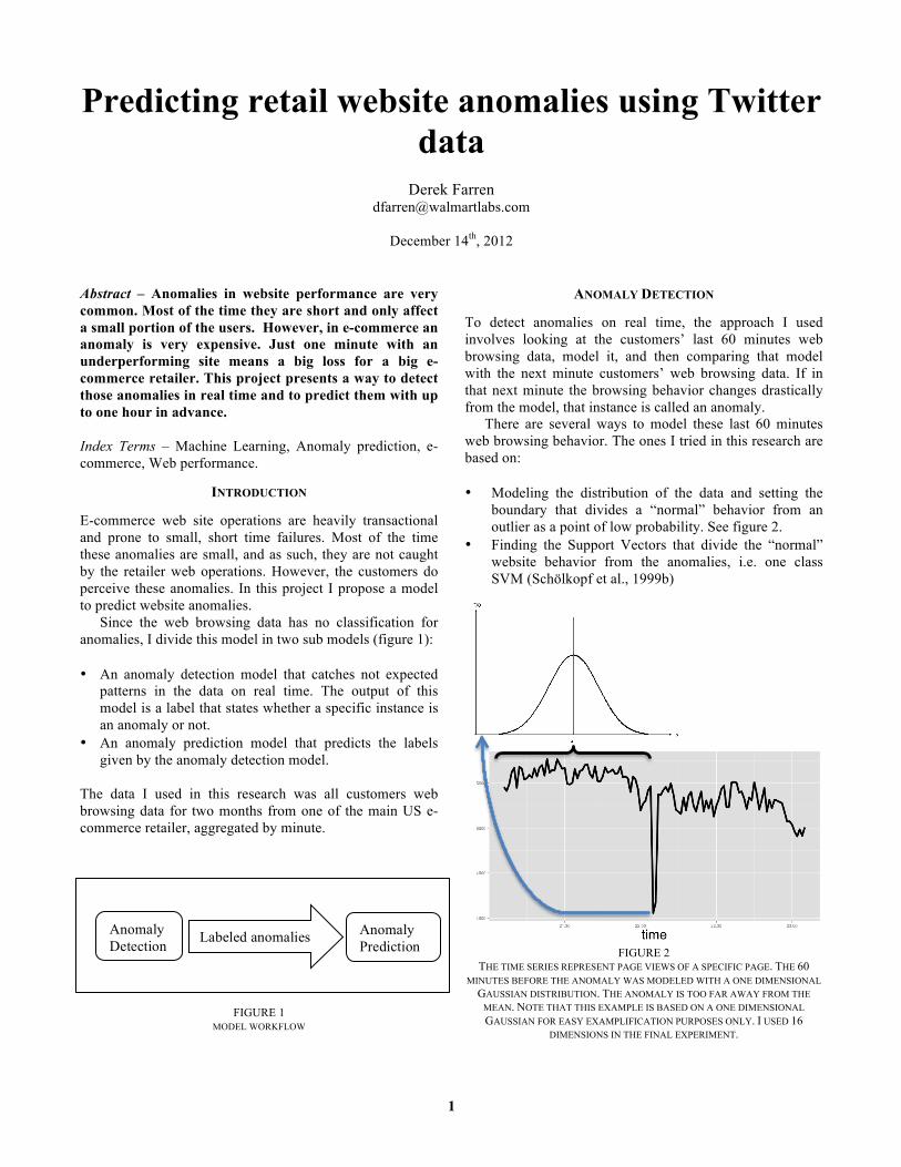
Since the web browsing data has no classification for anomalies, I divide this model in two sub models (figure 1): • An anomaly detection model that catches not expected

patterns in the data on real time. The output of this model is a label that states whether a specific instance is an anomaly or not.

• An anomaly prediction model that predicts the labels given by the anomaly detection model.

The data I used in this research was all customers web browsing data for two months from one of the main US e-commerce retailer, aggregated by minute.

FIGURE 1 MODEL WORKFLOW

ANOMALY DETECTION

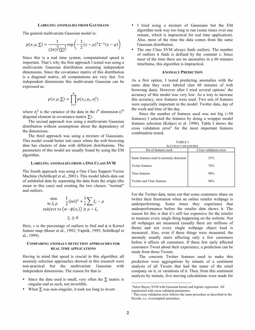
To detect anomalies on real time, the approach I used involves looking at the customers’ last 60 minutes web browsing data, model it, and then comparing that model with the next minute customers’ web browsing data. If in that next minute the browsing behavior changes drastically from the model, that instance is called an anomaly.

There are several ways to model these last 60 minutes web browsing behavior. The ones I tried in this research are based on:

• Modeling the distribution of the data and setting the

boundary that divides a “normal” behavior from an outlier as a point of low probability. See figure 2.

• Finding the Support Vectors that divide the “normal” website behavior from the anomalies, i.e. one class SVM (Schölkopf et al., 1999b)

FIGURE 2

THE TIME SERIES REPRESENT PAGE VIEWS OF A SPECIFIC PAGE. THE 60 MINUTES BEFORE THE ANOMALY WAS MODELED WITH A ONE DIMENSIONAL

GAUSSIAN DISTRIBUTION. THE ANOMALY IS TOO FAR AWAY FROM THE MEAN. NOTE THAT THIS EXAMPLE IS BASED ON A ONE DIMENSIONAL GAUSSIAN FOR EASY EXAMPLIFICATION PURPOSES ONLY. I USED 16

DIMENSIONS IN THE FINAL EXPERIMENT.

Anomaly Detection

Anomaly Prediction

Labeled anomalies

2

LABELING ANOMALIES FROM GAUSSIANS

The general multivariate Gaussian model is:

𝑝 𝑥; 𝜇,∑ =1

(2𝜋)!!|∑|

!!exp −

12𝑥 − 𝜇 !Σ!! 𝑥 − 𝜇

Since this is a real time system, computational speed is important. That’s why the first approach I tested was using a multivariate Gaussian distribution assuming independent dimensions. Since the covariance matrix of this distribution is a diagonal matrix, all computations are very fast. For independent dimensions this multivariate Gaussian can be expressed as:

𝑝 𝑥; 𝜇,∑ = 𝑝(𝑥!; 𝜇!,𝜎!!)!

!!!

where 𝜎!! is the variance of the data in the ith dimension (ith diagonal element in covariance matrix ∑).

The second approach was using a multivariate Gaussian distribution without assumptions about the dependency of the dimensions.

The third approach was using a mixture of Gaussians. This model would better suit cases where the web browsing data has clusters of data with different distributions. The parameters of this model are usually found by using the EM algorithm.

LABELING ANOMALIES FROM A ONE CLASS SVM

The fourth approach was using a One Class Support Vector Machine (Schölkopf et al., 2001). This model labels data out of unlabeled data by separating the data from the origin (the mean in this case) and creating the two classes: “normal” and outliers.

min          w, ξ, ρ                

12| 𝑤 |! +

1𝜈

𝜉! − 𝜌!

 

𝑠𝑢𝑏𝑗𝑒𝑐𝑡  𝑡𝑜   𝑤 ∙ 𝜙 𝑥! ≥ 𝜌 − 𝜉!

𝜉! ≥ 0  

Here, ν is the percentage of outliers to find and ϕ is Kernel feature map (Boser et al., 1992; Vapnik, 1995; Schölkopf et al., 1999).

COMPARING ANOMALY DETECTION APPROACHES FOR REAL TIME APPLICATIONS

Having in mind that speed is crucial in this algorithm; all anomaly selection approaches showed in this research were non-practical but the multivariate Gaussian with independent dimensions. The reason for that is:

• Since the data used is small, very often the ∑ matrix is singular and as such, not invertible.

• When ∑ was non-singular, it took too long to invert.

• I tried using a mixture of Gaussians but the EM algorithm took way too long to run (some times over one minute, which is impractical for real time application). Also, most of the time the data comes from the same Gaussian distribution.

• The one Class SVM always finds outliers. The number of outliers it finds is defined by the constant ν. Since most of the time there are no anomalies in a 60 minutes timeframe, this algorithm is impractical.

ANOMALY PREDICTION

As a first option, I tested predicting anomalies with the same data they were labeled (last 60 minutes of web browsing data). However after I tried several options1 the accuracy of this model was very low. As a way to increase this accuracy, new features were used. Two sets of features were especially important in the model: Twitter data, day of the week and time of the day.

Since the number of features used was not big (<50 features) I selected the features by doing a wrapper model features selection (Kohavi et al. 1996). Table I shows the cross validation error2 for the most important features combination tested.

TABLE I

ACCURACY MEASSURES Set of features used Cross validation error

Same features used in anomaly detection Twiter features Time features Twitter and Time features

53%

74%

90%

96%

For the Twitter data, turns out that some customers share on twitter their frustration when an online retailer webpage is underperforming. Some times they experience that underperformance before the retailer data shows it. The reason for this is that it’s still too expensive for the retailer to measure every single thing happening on the website. Not all webpages are measured (usually there are millions of them) and not every single webpage object load is measured. Also, even if these things were measured, the anomaly usually starts affecting only a few customers before it affects all customers. If these few early affected customers Tweet about their experience, a prediction can be made from those Tweets.

The concrete Twitter features used to make this prediction were aggregations by minute of a sentiment analysis of all Tweets that had the name of the retail company on it, or variations of it. Then, from this sentiment analysis by minute, five moving calculations were made for

1Naïve Bayes, SVM with Gaussian kernel and logistic regression. All regularized with cross-validated parameters. 2 This cross validation error follows the same procedure as described in the Results, i.e. oversampled anomalies.

3

the last 60 minutes (max, min, mean, standard deviation and median). This final dataset has five sentiment measures that represent the customer feelings about the retail company for the last moving 60 minutes.

I did the sentiment analysis by using the AFINN list (Finn Årup Nielsen, 2011). This is a list of the 2.477 most used words in the English language, with a corresponding sentiment score that goes from -5 to +5. For each Tweet, I matched the words to the ones in the AFINN list and added their score to get a final score. A final score of 0 means the tweet was neutral in terms of the author’s feeling about the retail company. If the score is positive, the author’s feeling about the retail company is positive. If the score is negative… well you get the idea.

Regarding the day of the week and hour of the day feature, the model performed the best when these features were dummy codded as categorical features instead of using numerical features.

The classes to predict were two:

• 1: there is at least one anomaly in the next hour • 0: there is no anomaly in the next hour. The model I used was a SVM with L1 regularization and Gaussian Kernels.

EXPERIMENT

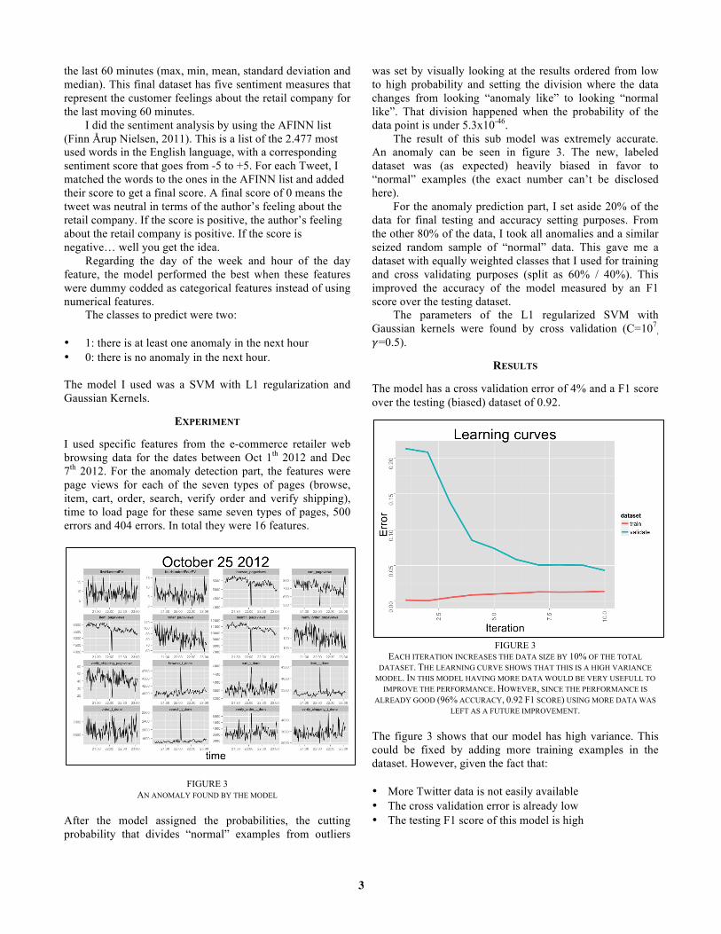
I used specific features from the e-commerce retailer web browsing data for the dates between Oct 1th 2012 and Dec 7th 2012. For the anomaly detection part, the features were page views for each of the seven types of pages (browse, item, cart, order, search, verify order and verify shipping), time to load page for these same seven types of pages, 500 errors and 404 errors. In total they were 16 features.

FIGURE 3 AN ANOMALY FOUND BY THE MODEL

After the model assigned the probabilities, the cutting probability that divides “normal” examples from outliers

was set by visually looking at the results ordered from low to high probability and setting the division where the data changes from looking “anomaly like” to looking “normal like”. That division happened when the probability of the data point is under 5.3x10-46.

The result of this sub model was extremely accurate. An anomaly can be seen in figure 3. The new, labeled dataset was (as expected) heavily biased in favor to “normal” examples (the exact number can’t be disclosed here).

For the anomaly prediction part, I set aside 20% of the data for final testing and accuracy setting purposes. From the other 80% of the data, I took all anomalies and a similar seized random sample of “normal” data. This gave me a dataset with equally weighted classes that I used for training and cross validating purposes (split as 60% / 40%). This improved the accuracy of the model measured by an F1 score over the testing dataset.

The parameters of the L1 regularized SVM with Gaussian kernels were found by cross validation (C=107

, 𝛾=0.5).

RESULTS

The model has a cross validation error of 4% and a F1 score over the testing (biased) dataset of 0.92.

FIGURE 3

EACH ITERATION INCREASES THE DATA SIZE BY 10% OF THE TOTAL DATASET. THE LEARNING CURVE SHOWS THAT THIS IS A HIGH VARIANCE

MODEL. IN THIS MODEL HAVING MORE DATA WOULD BE VERY USEFULL TO IMPROVE THE PERFORMANCE. HOWEVER, SINCE THE PERFORMANCE IS

ALREADY GOOD (96% ACCURACY, 0.92 F1 SCORE) USING MORE DATA WAS LEFT AS A FUTURE IMPROVEMENT.

The figure 3 shows that our model has high variance. This could be fixed by adding more training examples in the dataset. However, given the fact that:

• More Twitter data is not easily available • The cross validation error is already low • The testing F1 score of this model is high

4

I decided to leave it as it is and plan on adding more data as a future improvement.

An important finding of this applied research is that the set of features that have the most important predictive value are the time related features3 (day of week and time of day). It seems like most of the anomalies in the webpage happen around 10PM and 4AM.

CONCLUSIONS

Anomalies on an e-commerce website can be accurately detected in real time. Most of the time modeling the web features to be measured (page views, time to load, etc.) as multivariate Gaussian with independent dimensions is good enough to have a very accurate real time model. Predicting anomalies using the same web measures used to label them is not recommended. The best approach to predict web pages anomalies showed to be selecting new features from other sources. In my experiment, Twitter data, day of week and time of day had a strong predictive value for anomalies.

REFERENCES

[1] B. Schölkopf, J.C. Platt, J. Shawe-Taylor, A.J. Smola, and R.C.

Williamson, “Estimating the support of a high-dimensional distribu- tion,” Neural Computation, vol. 13, no. 7, pp. 1443–1471, 2001.

[2] B. E. Boser, I. M. Guyon, and V. N. Vapnik. A training algorithm for optimal margin classifiers. In D. Haussler, editor, Proceedings of the 5th Annual ACM Workshop on Computational Learning Theory, pages 144–152, Pittsburgh, PA, 1992. ACM Press.

[3] V. Vapnik. The Nature of Statistical Learning Theory. Springer Verlag, New York, 1995.

[4] B. Schölkopf, C. J. C. Burges, and A. J. Smola. Advances in Kernel Methods — Support Vector Learning. MIT Press, Cambridge, MA, 1999.

[5] Finn Årup Nielsen, "A new ANEW: Evaluation of a word list for sentiment analysis in microblogs", Proceedings of the ESWC2011 Workshop on 'Making Sense of Microposts': Big things come in small packages 718 in CEUR Workshop Proceedings : 93-98. 2011 May.

[6] R. Kohavi, G.H. John, "Wrappers for feature subset selection", Artificial Inteligence 1997 273-324

AUTHOR INFORMATION

Derek Farren, Data Scientist @WalmartLabs.

3 Table I has the details.