Embed Size (px)
Citation preview
Predicting Lotto Numbers
A natural experiment on the gambler’sfallacy and the hot hand fallacy
Claus B. Galbo-Jørgensen
University of Copenhagen, Department of EconomicsØster Farimagsgade 5, building 26, 1353 København K, Denmark
e-mail: [email protected]
Sigrid Suetens
CentER - Department of Economics, Tilburg UniversityPO Box 90153, 5000 LE Tilburg, The Netherlands
e-mail: [email protected]
Jean-Robert Tyran
University of Vienna and University of Copenhagen, Department of EconomicsHohenstaufengasse 9, A-1010 Vienna, Austria
e-mail: [email protected]
Abstract
We investigate the “law of small numbers” using a data set on lotto gambling that allows us
to measure players’ reactions to draws. While most players pick the same set of numbers week
after week, we find that those who do change, react on average as predicted by the law of small
numbers as formalized in recent behavioral theory. In particular, players tend to bet less on
numbers that were drawn in the last week, as suggested by the “gambler’s fallacy”, and bet
more on a number if it was frequently drawn in the recent past, consistent with the “hot hand
fallacy”.
JEL Codes: D03, D81, G02
Keywords: behavioral economics, decision biases, gambler’s fallacy, hot hand fallacy, lotto gambling
Date: December 14, 2012
1 Introduction
Drawing the right inference from observing noisy data is difficult. People even tend to see patterns in
data when, in fact, there are absolutely none. This paper focuses on two — apparently contradictory
— fallacies in inference from noisy data that have been found to be pervasive in the literature
(Tversky and Kahneman, 1971). One is the “gambler’s fallacy” (GF) according to which people
tend to believe in frequent reversals, i.e. that a particular event is less likely to occur because it
occurred recently. In state lotteries, for example, after a number has been drawn, the amount bet on
that number falls sharply (Clotfelder and Cook, 1993; Terrell, 1994), and roulette players expect
that a black number is “due” after observing a sequence of red numbers (Croson and Sundali,
2005).1 The other is the “hot hand fallacy” (HHF) according to which people believe in the
continuation of a trend, i.e. that a particular event is more likely to occur because a recent streak
of such events occurred. A much-cited case in point is that bets on basketball players who scored
unusually well in the recent past tend to be too high (Gilovich et al., 1985; Camerer, 1989). And
Guryan and Kearney (2008) provide evidence for a “lucky store effect”, the observation that lotto
vendors sell many more tickets if they have sold a ticket that won a large prize a week earlier.2
A theoretical model by Rabin and Vayanos (2010) (henceforth RV) shows that the two appar-
ently contradictory fallacies can be reconciled with reference to the “law of small numbers” (LSN
Tversky and Kahneman, 1971).3,4According to the LSN, people hold the fallacious belief that small
samples should be representative of the population and should therefore “look like” large samples.
RV show that a person who falls prey to the GF in the short run is also prone to develop the HHF
in the long run. We provide supportive evidence for such “fallacy reversal” using data from a state
lottery. The unique aspect of our data is that we can track players’ choices (the numbers they bet
on) over time. While others have used controlled data from state lotteries before, we shed new light
on the relation of these fallacies by being the first to study how individual players react with their
number picking to recent draws.
The intuition behind fallacy reversal is as follows.5 A person who believes that small samples
should “look like” large samples expects frequent reversals in short random sequences, and thus
1Frequent reversals have also been observed in various laboratory experiments where participants are asked togenerate a random sequence as in a coin toss (e.g., Bar-Hillel and Wagenaar, 1991; Rapoport and Budescu, 1997).
2False hot hand beliefs also arise in laboratory experiments with an ambiguous data-generating process(Offerman and Sonnemans, 2004) or among participants who let “experts” bet for them on outcomes of randomdraws (Huber et al., 2010). Powdthavee and Riyanto (2012) show that lab participants are even willing to pay forthe (transparently useless) advice of “experts”.
3See also Rabin (2002).4In fact, the Marquis de Laplace (1812) had already suggested that both fallacies (he calls them illusions) are
likely to occur in lotto gambling: “When a number in the lottery of France has not been drawn for a long time thecrowd is eager to cover it with stakes. They judge since the number has not been drawn for a long time that it oughtat the next drawing to be drawn in preference to others. So common an error appears to me to rest upon an illusion(...). By an illusion contrary to the preceding ones one seeks in the past drawings of the lottery of France the numbersmost often drawn, in order to form combinations upon which one thinks to place the stake to advantage. But (...)the past ought to have no influence upon the future.” Cited after Truscott and Emory, 1902: 161f.
5See Appendix A.1 for an interpretation of the model by RV in terms of lotto play.
1
falls prey to the GF in the short run. If such a person is uncertain about the true probability
underlying a sequence of events, she starts to doubt about the true probability when observing a
long streak because this observation does not correspond to what she believes a random sequence
should look like. As a consequence, this person revises her estimate of the true probability, starts
to believe in the continuation of the streak, and thus develops the HHF.6 Uncertainty about the
true probability is key for a fallacy reversal to occur according to this theory. Believers in the LSN
who are absolutely certain about the true probability underlying the data-generating process are
predicted to continue exhibiting the GF without developing the HHF when observing long streaks.7
The LSN as modeled by RV not only reconciles gambling behavior and betting in sports markets,
but may also provide a unifying framework to account for several anomalies observed in financial
markets. One of these anomalies is that asset prices underreact to news in the short run and, as
a consequence, returns show momentum, whereas they overreact over long time horizons, leading
to reversal in returns in the long run.8 In a nutshell, the reasoning is as follows. If many investors
are prone to the GF, and believe that short sequences of unexpectedly high earnings will quickly
reverse in the future, stock prices will underreact to news about earnings. The same investors, if
uncertain about the process behind earnings sequences, attribute long streaks of unexpectedly high
earnings to an underlying fundamental and expect such streaks to continue, leading to overreaction
of stock prices.9 However, among investors who are confident that earnings are iid, underreaction
persists and may even become stronger, the longer the streak. Along the lines of this intuition,
Loh and Warachka (2012) show that stock returns underreact to “news” (earnings surprises) in the
short and long run.10
We study the GF and the HHF among lotto players by inferring players’ beliefs about winning
numbers from the numbers they choose on their lotto tickets, and by relating these choices to
6A similar pattern of fallacy reversal in an iid sequence is predicted by Barberis et al. (1998) who assume thatinvestors switch between two states of mind about the world depending on the arrival of “news” (observed earningssurprises). The model predicts that investors are more likely to expect a reversal of a trend the longer a streaklasts, but empirical evidence suggests this is not necessarily the case. For example, Croson and Sundali (2005) andAsparouhova et al. (2009) show that the proportion of GF bets may increase with streak length.
7Uncertainty about the true probability also seems to be key in practice. Asparouhova et al. (2009) ask participantsin a lab experiment to predict the next observation in a random-walk process. The authors show that the HHFbecomes more prevalent (compared to the GF) as subjects perceive the data-generating process to be less random.Lab experiments in psychology also show that the GF is mostly observed when events are believed to be totallyrandom while the HHF arises when events are perceived to be at least partly driven by a systematic factor, involving,for example, human skill (see Oskarsson et al., 2009, for a review). Guryan and Kearney (2008) also provide anexplanation along these lines for their “lucky store effect”.
8De Bondt and Thaler (1985, 1987) and Jegadeesh and Titman (1993) are seminal papers documenting long-runoverreaction and short-run momentum, respectively. Poterba and Summers (1988) and Cutler et al. (1991) showthat returns in financial markets are positively autocorrelated in the short run and negatively autocorrelated inthe long run. More recent evidence for underreaction to earnings announcements in the short run comes fromCohen and Frazzini (2008), DellaVigna and Pollet (2009), and Hirshleifer et al. (2009).
9These aggregate patterns may additionally be driven by biases in the processing of private information amonginvestors (e.g. Daniel et al., 1998; Hong and Stein, 1999). Such biases are unlikely in lotto gambling given that allinformation about outcomes of lotto draws is public.
10The authors suggest that overreaction to streaks of high earnings is absent because investors are confident thatthe long-term distribution of earnings surprises is iid.
2
recent histories of lotto draws. Since people who play lotto are also likely to invest in lotto-type
stocks, such as low-priced stocks with high idiosyncratic volatility and skewness (Kumar, 2009), it
seems reasonable to assume that the same biases may play a role in both lotto gambling and stock
markets. But inferring the existence of such biases and how they may relate using financial market
data is fraught with difficulties. A particularly important problem is that the data-generating
process in financial markets is not known to the researcher but has to be somehow estimated.
Financial market data do not provide a clean test environment because these data are not only
driven by randomness but also by ability, skill, or other systematic factors that are often difficult
to measure. For example, long streaks of unexpectedly high earnings in a firm can be due to
chance but they can also have a more fundamental cause, so it is not clear whether investing in
stocks with a long history of high earnings should be seen as a hot hand fallacy or as a hot hand
reality.11 In contrast, lotto gambling is an ideal test environment to study these fallacies and how
they relate. It provides a natural experiment because lotto draws follow a known, truly random
process (with a fixed probability for each number), and are thus independent and truly exogenous.
In fact, the true randomness of the game is tightly controlled (often by government regulation) and
made transparent to players (e.g., by drawing balls from an urn and by airing the draws on TV).
A key advantage of our data is that we can track individual players over time. The data come
from lotto played over the Internet in Denmark where the law requires gamblers to be uniquely
identified. This identification allows us to construct variables measuring how an individual player
reacts — adjusts his or her number choices — to recent draws. We are therefore not only able to
see if a bias is present for the average player but we can also test if players prone to GF are prone
to HHF as streaks get longer.12
We find strong evidence of GF. Players place on average two percent fewer bets on numbers
drawn in the previous week compared to numbers not drawn, as long as those numbers are not
“hot”. We also find evidence of the HHF. Players bet more money on numbers as they get “hotter”,
i.e. as the numbers have won more often in the recent past. An individual-level analysis shows that
9.2% of the players are biased in the sense that they significantly react to the previous week’s
drawings. Among these players, 64% place their bets in line with GF. They decrease their bets
on last week’s winners. Our analysis shows that the two fallacies are systematically related, as
predicted by RV. We find that a majority (57%) of these GF players are consistent with HHF.
These players tend to increase their bets on last week’s winners the “hotter” these winners are.
Finally, we also show that being biased is costly. The cost comes in two guises. First, biased
players lose more money because they buy more tickets. Second, biased players win less money
11For example, persistence has been observed in the performance of mutual funds (Hendricks et al., 1993; Carhart,1997) and superior hedge funds (Jagannathan et al., 2010). Similar problems apply to data from sports. A belief in hothands is not necessarily fallacious but may be “real”. See Bar-Eli et al. (2006) for an overview and Yaari and David(2012) for a recent study using data on bowling.
12Sundali and Croson (2006) also use individual-level data to investigate the two fallacies. These authors show thatplayers who exhibit the GF, i.e. bet less on the winning numbers of the most recent spin, are more likely to increasetheir bets after winning and vice versa. They are thus more likely to believe to have a hot hand with respect to theamount bet.
3
than random players if they happen to win because common biases induce coordinated betting
which is costly given the pari-mutuel structure of lotto.
The paper is organized as follows. Section 2 describes the lotto data and defines the main
variables of interest. Section 3 analyzes the aggregate reaction of lotto players to the recent drawing
history of lotto numbers. Section 4 uses individual-level data to investigate the relation between
the two biases. Section 5 shows that being biased comes at a monetary cost. Section 6 concludes.
2 The data
We analyze data from lotto played on Saturdays in Denmark over the Internet (henceforth lotto
for short) covering 28 weeks in 2005. Lotto is organized by a state monopoly (Danske Spil). Every
Saturday, 7 balls are drawn from an urn containing 36 balls numbered from 1 to 36, which is aired
on state TV. The price of a lotto ticket is about EUR 0.40 (DKK 3).13
The payout rate is set to 45% by law and the remainder of the revenues is earmarked for “good
causes” or goes to the general government budget. Lotto has a parimutuel structure as the payout
rates are fixed per prize category and the prize money per category is shared among the winners
in that category. One quarter of all payouts are reserved for the jackpot (7 correct numbers), and
there are four graded prizes for having selected fewer correct numbers. If no-one wins the jackpot,
it is rolled-over to the next week. In our data set, the average jackpot was about EUR 534’000
(4 million DKK), and the highest jackpot was 1.4 million EUR (10.2 million DKK). Prizes above
DKK 200 are subject to a special tax of 15% but are otherwise exempt from income tax.
Lotto is normally played in Denmark by purchasing hard-copy lotto tickets in vending booths
like drugstores and supermarkets. Since 2002, lotto can also be played over the Internet. Lotto
numbers can be picked in various ways in Denmark. Traditionally, players manually select 7 out of
36 numbers on each ticket they buy. However, we analyze numbers picked in “Systemlotto”. Here,
players select between 8 and 31 numbers manually and let the lotto agency choose combinations
of 7 out of these numbers.14 Our data has been provided directly by the state lottery agency and
is unlikely to contain any error. All players in our dataset are identified by a unique ID-number
which allows us to track the choices of players over time. In total, 189’531 persons have played
lotto over the Internet at least once in the second half of 2005. More than half of these (100’386)
manually select their numbers in the traditional way, and 25’807 select numbers using Systemlotto.
The reason for focusing on Systemlotto rather than the traditional manual selection is that
Systemlotto is more appropriate to capture the belief in one’s ability to predict winning numbers
and the reaction of number picking to recent draws. In fact, in Systemlotto players choose numbers,
rather than combinations of numbers, as in the traditional manual selection. They choose fewer
unique numbers than players who select in the traditional way which suggests that they are more
13The following describes the rules of lotto at the time the data was collected. The prize structure has been modifiedsince to yield higher jackpots.
14Other ways to play are “Quicklotto” where all numbers are selected randomly by the lotto agency and “Lucky-lotto” where players select up to 6 numbers manually and let the lotto agency choose the remaining numbers.
4
likely to believe that a particular number is going to win. To illustrate, Systemlotto players pick
less than half among the 36 available numbers (14 numbers in an average week, 8 in a modal
week), while in manual selection players pick most available numbers (29 in an average week, 32
in a modal week). A particular focus of our study is on how players react to the recent history of
draws including an analysis of how they react to a number being a more or less frequent winner in
the recent past. While observing that particular numbers win repeatedly is relatively likely, this is
extremely unlikely for combinations of numbers.15
An advantage of our data set compared to laboratory data is that it reflects behavior of a
heterogeneous pool of people and behavior is observed in a “natural” situation. In fact, lotto is quite
popular in Denmark. For example, according to the lotto agency, about 75% of the adult Danish
population have played lotto at least once. Yet, Systemlotto players are clearly not representative
for the Danish population or even for the pool of internet lotto players. People playing Systemlotto
buy on average about twice as many tickets as other internet players (29 vs. 14 tickets per week;
the medians are 19 and 10, respectively). Systemlotto is also especially popular with male players:
82% of the players are male compared to 73% for other selection devices.16
2.1 Dependent variable
Our empirical strategy is to make inferences about the (unobservable) belief in the ability to predict
winning lotto numbers more accurately than pure chance from observable reactions to previous
drawings. That is, we infer that players think recently drawn numbers are more likely to win if
they systematically prefer them and vice versa if they avoid them. A player is said to be more
confident that a particular number is going to win if he or she places more bets on it (i.e. buys
more tickets including this number). More specifically, we define a variable “weight” showing how
much money is bet on a number relative to other numbers. We then define a variable “reaction”
measuring how much more a player is confident that a particular number is going to win conditional
on previous draws. More specifically, “reaction” shows the change in “weight” placed on a particular
number.
This empirical approach is rather straightforward but not perfect because it can only detect
some of the fallacies that may be present. To illustrate, consider a player who is prone to the GF,
i.e. believes that if number x won last week it is less likely to win this week. Our analysis can only
uncover that bias if the player actually picked number x in the first week. Given that players in
our sample only bet on a subset of numbers (14 out of 36 numbers in an average week), we are
likely to underestimate the bias.
15While there are only 36 numbers, there are about 8 million ways to combine 7 out of 36 numbers (36!/(7!(36−7)!) =8′347′680). The probability that the same combination occurs twice in a row is therefore about 1 in 70 trillion (7 x10¹³) in Danish lotto. Curiously enough, the same six numbers were drawn twice in a row in the Bulgarian lotto inSeptember 2009. This event was considered to be so unlikely that it prompted the Bulgarian government to initiatean investigation for manipulation of the game.
16Male players buy significantly more tickets than female players, irrespective of the selection device, and System-lotto players buy significantly more tickets than other players, irrespective of the gender (p = 0.000 in Mann-Whitneyrank-sum tests).
5
Our empirical proxy for how confident a player is in his prediction is how much money he bets
on a particular number relative to other numbers. Constructing this proxy is not entirely trivial
because it depends on the number of “sets” of numbers, the number of tickets generated from each
set, and the number of lotto numbers contained in each set. Recall that in Systemlotto, players
pick one or more sets containing 8 to 31 numbers. For each chosen set, the lotto agency generates
at least 8 tickets with different combinations (of subsets) of the chosen numbers.17 To illustrate
the construction of our proxy, consider the following examples.
Example 1 Player A chooses a set of 10 numbers and Player B chooses a set of 24 numbers. Both
A and B buy 120 tickets generated out of their chosen sets.
Example 2 Player C chooses a set of 10 numbers from 1 to 10 and a set of 10 numbers from 5 to
14. For each set, 8 tickets are generated. Player C thus buys 16 tickets in total.
In example 1, both players buy the same number (120) of tickets. Yet, it is plausible to assume
that player A is more confident that (some of) his 10 numbers are going to win than player B who
picks 24 numbers. Our proxy therefore gives each of the 10 numbers chosen by player A a larger
weight (of 1/10) than each of the 24 numbers chosen by player B (1/24). In example 2, player C
chooses two sets which partly overlap since the numbers 5 to 10 are elements of both sets. It seems
plausible to assume that player C is more confident that one of the numbers contained in both sets
(5 to 10) is going to win than one of the numbers chosen in only one of the sets (1 to 4 and 11
to 14). Our proxy therefore gives more weight to numbers occurring in overlapping sets than to
numbers occurring in only one set.
To compare weights across players, we normalize the number of times lotto number j is picked
by player i in week t by the total number of lotto numbers picked by player i in week t across
all sets. This variable sums to 1 across all lotto numbers for each i and each t and thus provides
information about the relative weight players put on particular numbers. We refer to this variable
as Weightijt and define it as follows for lotto number j, player i and week t:
Weightijt =# of times lotto number j is picked in week t by player i
# of lotto numbers picked in week t by player i(1)
We are now ready to define the key variable Reactionijt which shows how players change relative
weights on numbers from period to period. Again, the definition of this variable requires some
care because some (i.e. low) numbers are generally more popular than others, and some (perhaps
idiosyncratically “lucky”) numbers are more popular with particular players than others. In the
construction of the variable Reactionijt, we therefore control for “baseline” choices of players, i.e.
17The total number of tickets/combinations generated by Systemlotto out of a set of chosen numbers is positivelyrelated to the total number of lotto numbers a player chooses in the set. The exact relation depends on which ofthree “systems” players use to generate tickets/combinations. See Appendix A.2 for details.
6

Table 1: Summary statistics of dependent variable Reactionijt
Minimum -0.12500Maximum 0.12500Mean 0.00000Standard Deviation 0.02247Number of data points 2’826’180
Notes: The median and first and third quartile are all equal to zero.
numbers that players choose irrespective of the recent history of drawings by differencing them out.
To illustrate, consider a player who, for example, always chooses lotto number 2 in combination
with other (time-varying) numbers. Suppose number 2 is drawn in week t− 1. If we do not correct
for the player’s idiosyncratic preference, we would wrongly conclude that the player exhibits the
HHF. This consideration is especially important given that low numbers are more popular than
high numbers. For example, the lowest 5 numbers (1 to 5) are picked more than 30% more often
than the highest 5 numbers (32 to 36).18 Therefore, the dependent variable Reactionijt for lotto
number j, player i and week t is defined as:
Reactionijt = ∆Weightijt = Weightijt −Weightijt−1 (2)
A player is said to “avoid”, “move away from” or “bet less” on a number in period t if
Reactionijt < 0 and vice versa for Reactionijt > 0.
A majority of players in our dataset pick the same numbers week after week. In fact, out of the
25’807 Systemlotto players in our dataset, 17’318 have at least two consecutive observations such
that Reactionijt can be measured at least once. Of these, 10’434 players do not change their weight
on numbers at all, meaning that for these players Reactionijt = 0 for all j and t. About a quarter of
players in our data set (6’884) pick different numbers in consecutive weeks, i.e. have Reactionijt 6= 0
for at least one j in one t, and our analysis below is therefore based on these players.
Table 1 provides summary statistics on the dependent variable Reactionijt. By construction,
Reactionijt varies between -0.125 and 0.125 with a mean of 0. Intuitively, the symmetric range
results from the normalization and the fact that for every move toward a number there is a move
away from another number or other numbers of the same absolute size. The reason why the
maximum is equal to 0.125 and the minimum to -0.125 is that at least 8 tickets are generated
from each set and the maximum weight of a particular number is therefore 1/8 (= 0.125). Hence,
the maximum absolute change in weight — changing from a weight of zero to one of 1/8 or the
other way around — is 0.125. The median of Reactionijt is equal to zero and the interquartile
range is [0,0] since most players do not change their numbers. The statistics show there is certainly
no tendency for players to move away from (Reactionijt < 0) or toward (Reactionijt > 0) lotto
numbers. In other words, there are no pure time trends in number picking. However, as shown
next, the extent to which players avoid or prefer numbers is significantly related to outcomes of
18The popularity of the lotto numbers is shown in Appendix A.3.
7
recent drawings.
2.2 Independent variable
Our aim is to study whether players systematically react to drawings in previous weeks and, if so,
whether players who fall prey to the GF also develop the HHF. To test for the presence of GF, i.e.
whether players bet less on numbers drawn in the previous week, we define the variable Drawnjt−1
as follows:
Drawnjt−1 =
{
0 if number j has not been drawn in week t− 1,
1 if number j has been drawn in week t− 1.(3)
To study whether the HHF is present, we test whether players bet more on “hotter” numbers.
More specifically, we test whether players bet more on numbers that have been drawn frequently
in the past 6 weeks, given that the number has been drawn in the previous week. Note that this
frequency is conditional on observing a draw in t− 1. Thus, our measure serves to discuss whether
players bet more or less on numbers that have been drawn in week t− 1, depending on how often
the number was drawn in the 5 preceding weeks. We use this measure of “hotness” rather than
a literal “streak”, i.e. the number of consecutive weeks a number has been drawn because long
streaks are rare by the nature of randomness. In our sample, the maximum length of weeks with
consecutive draws of a particular number is 4, and such a streak occurs only once.19 We consider
the conditional frequency of draws in the previous 6 weeks because looking back further has no
statistical explanatory power.20
In summary, our second independent variable Hotnessjt−1 measures how often number j has
been drawn in weeks t− 1 to t− 6, given it has been drawn in week t− 1.
Hotnessjt−1 =
{
kif number j has been drawn k times in weeks t− 1 to
t− 6, conditional on being drawn in week t− 1.(4)
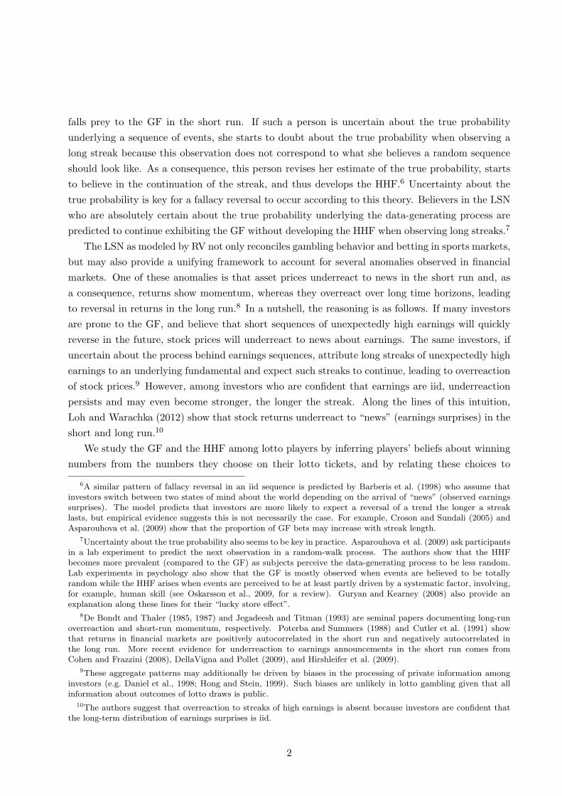
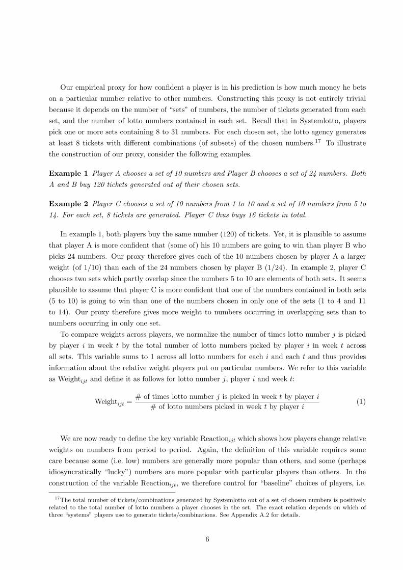
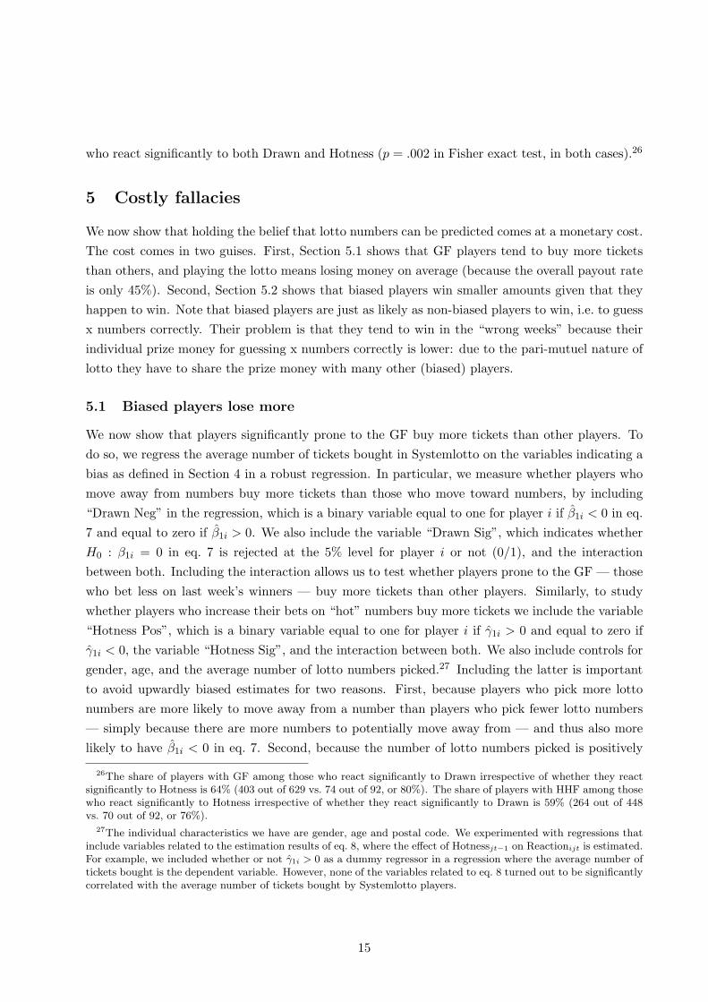
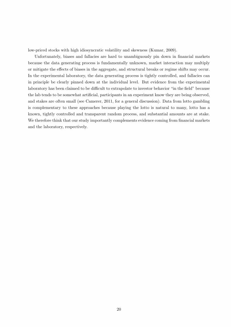
Figure 1 shows that the observed conditional frequency that numbers are drawn k times over
six weeks in our sample matches the expected frequency closely. For example, we observe 61 cases
where a number has been drawn exactly once in the 196 (= 7 numbers times 28 weeks) cases where
a number has been drawn while 66 such cases are expected. Note that it is extremely unlikely that
a number is drawn in all six weeks. The probability of observing this event is .00005 (= (7/36)6),
and it is not observed in our dataset. Unsurprisingly, we cannot reject the hypothesis that lotto
19The expected probability that a streak of length k occurs is 29/36 ∗ (7/36)k. In an earlier version of this paper,we use “streaks” rather than the indicator of “hotness” in our analysis. The results are qualitatively the same butstatistically less powerful.
20More specifically, we regress Reactionijt on Drawnjt−1, lags of Drawnjt−1 and interactions between Drawnjt−1
and lags of Drawnjt−1. Interactions are included in order to allow for different reactions depending on whether thenumber has been drawn in the previous week (see Table A1 in the Appendix for the regression results).
8
Figure 1: Expected and observed frequencies of numbers drawn over six consecutive weeks
66.49
80.24
38.74
9.35
1.13
.05
61
90
37
71
0020
4060
8010
0E
xpec
ted/
Obs
erve
d F
requ
ency
1 2 3 4 5 6Hotness
Expected FrequencyObserved Frequency
Notes: The chart shows for 196 number draws (7 lotto numbers times 28 weeks) expected and observed frequenciesthat numbers are drawn k times in weeks t − 1 to t − 6 given they have been drawn in week t − 1. The expectedfrequency a number is drawn k times in 6 weeks given it has been drawn once in 6 weeks is equal to the probability
that a number is drawn k − 1 times in 5 weeks, so equal to5!
(k − 1)!(5− (k − 1))!
(
7
36
)k−1 (29
36
)6−k
(k > 0).
drawings are truly random, since observed and expected counts are not different according to a
Chi-square test (χ2 = 2.37 whereas the critical value is 3.84).
3 Aggregate reaction to recent drawings
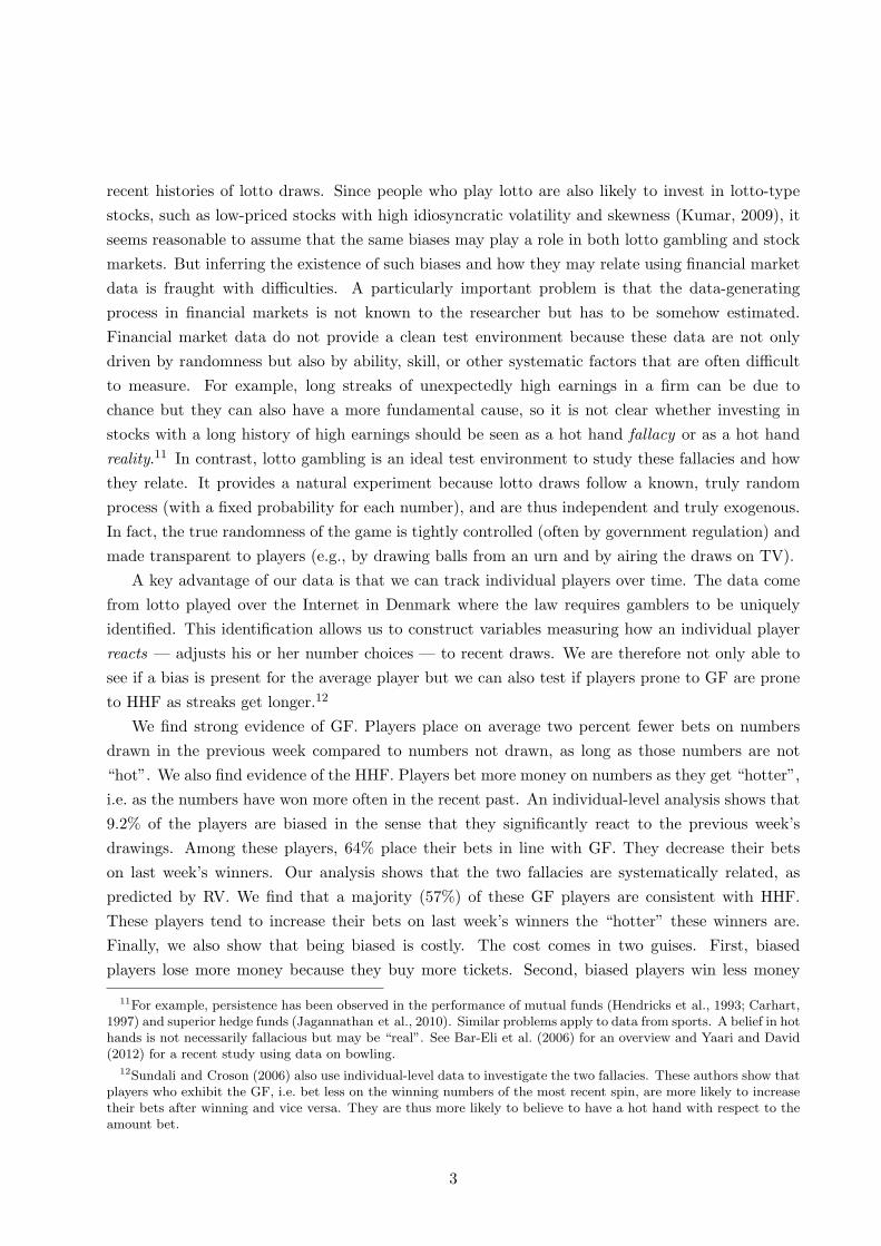
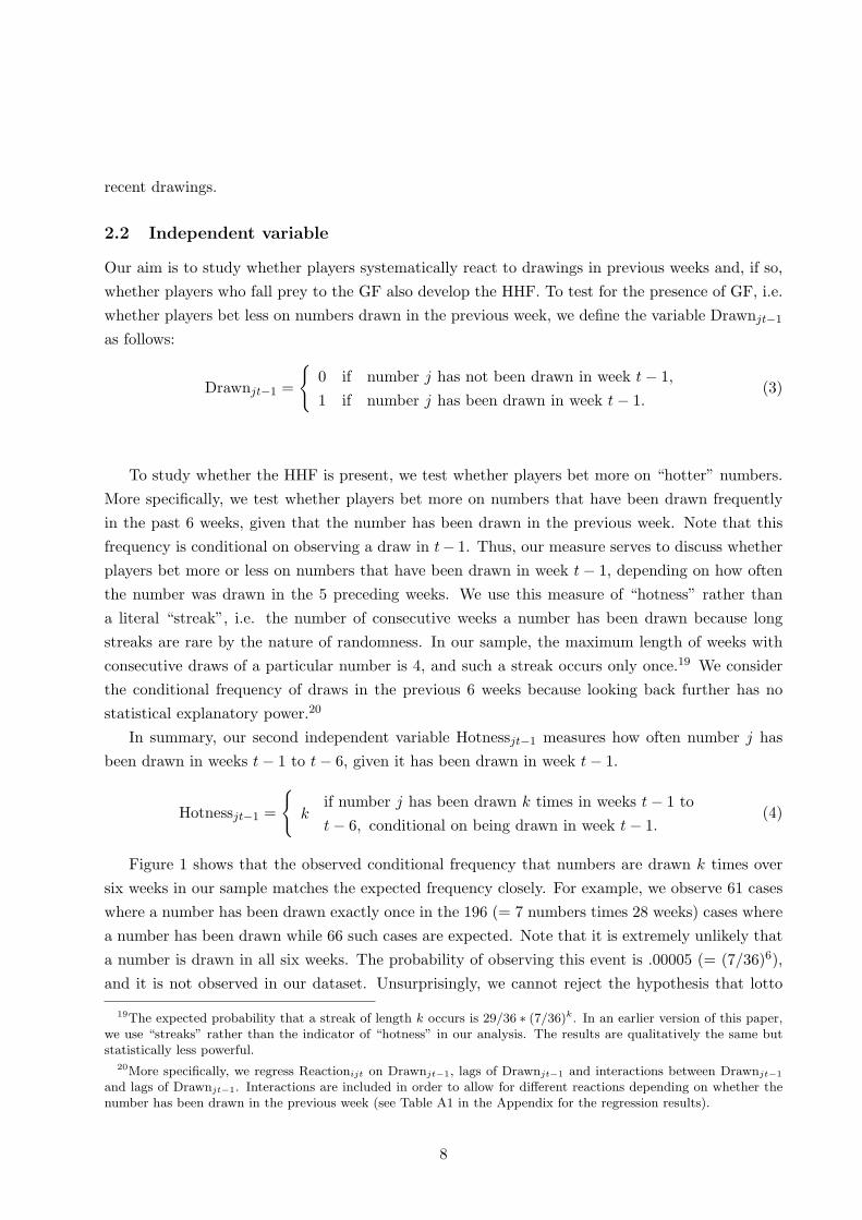
This section analyzes how players react to recent drawings by reporting the results from pooled
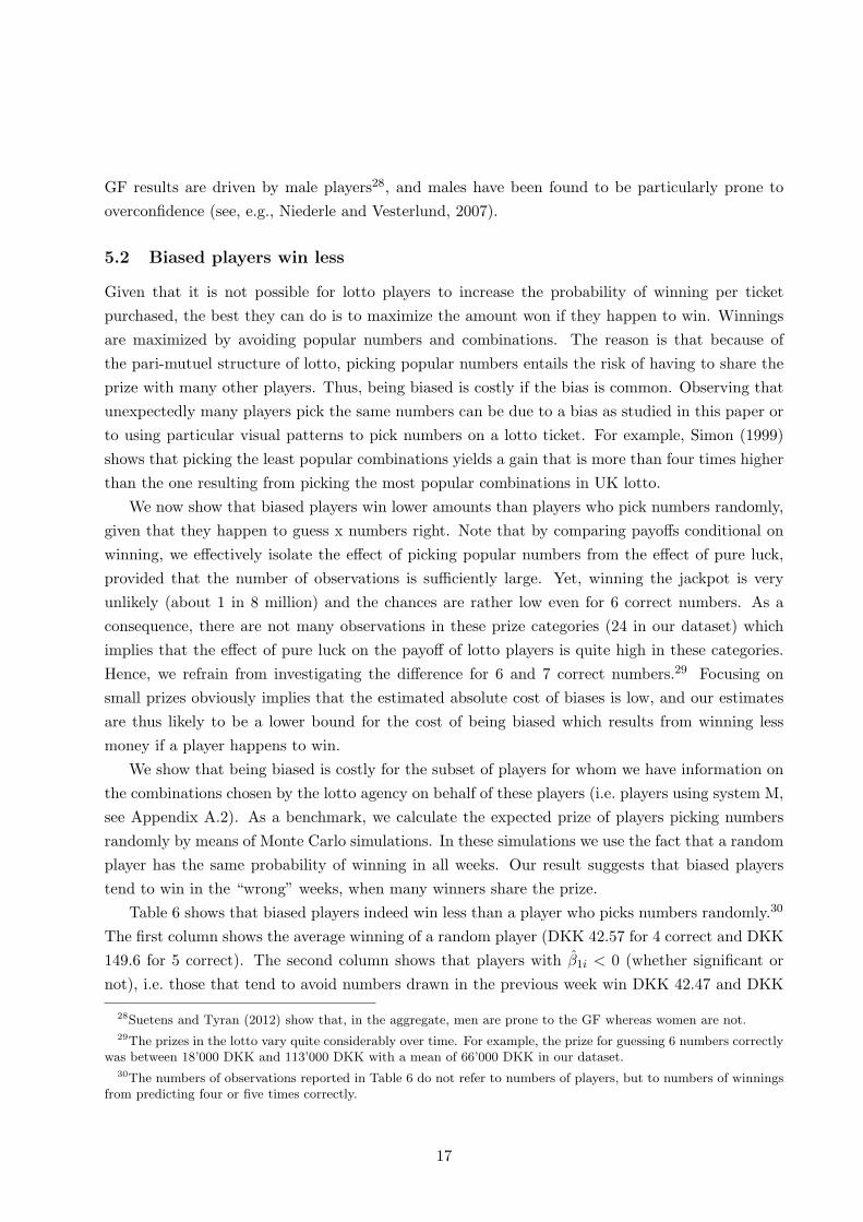
regressions to be explained in more detail below. Figure 2 summarizes the result. Panel (a) shows
that in the aggregate, players bet less on numbers that have been drawn (=1) in the previous week
(week t − 1) than on numbers that have not (=0). Translated into changes in bets, there are 2%
fewer bets on numbers drawn in the previous week than on numbers not drawn.21 This finding
provides support for the claim that the GF is a systematic bias in lotto gambling. Note that panel
(a) shows the unconditional reaction, i.e. the estimate here is independent of how “hot” the number
drawn was.22 Panel (b) shows the average reaction to a draw in week t − 1 as a function of the
hotness of the drawn number, i.e. how often the number has been drawn in the recent past (weeks
21This number is in the same ballpark as the one found in the lab by Asparouhova et al. (2009). They find that,on average, players reduce their probability estimate of continuation by approximately 0.9% for each unit increase instreak length for (short) streaks of length up to three.
22The weighted average “hotness” of numbers drawn in the previous week is about 1.17.
9
Figure 2: Average reaction as a function of the recent drawing history
(a) Function of Drawn in t-1
−.0
006
−.0
004
−.0
002
0.0
002
.000
4A
vera
ge r
eact
ion
0 1Drawn in Week t−1
(b) Function of Hotness in t-1 to t-6
−.0
006
−.0
004
−.0
002
0.0
002
.000
4A
vera
ge r
eact
ion
1 2 3 4 5Frequency Number Drawn in Weeks t−1 to t−6
Notes: Panel (a) shows the average of Reactionijt across all i, j, and t for a lotto number that has been drawn inweek t−1 (=1) or was not drawn (=0). Panel (b) shows the average of Reactionijt for a number that has been drawnin week t− 1 depending on how often the number was drawn in weeks t− 1 to t− 6. Level 1 on the horizontal axisindicates that the number was drawn only in week t− 1 but not so in weeks t− 2 to t− 6; level 2 indicates that thenumber was drawn in week t − 1 and in one of the earlier (t − 2 to t − 6) weeks; level 3 indicates that the numberwas drawn in week t− 1 and in two of the earlier weeks; and so on.
t − 1 to t − 6). The benchmark level for comparison is zero in both panels. A zero reaction in
the aggregate results if none of the players are biased (and there is some noise) or if biases are
present but cancel each other out. Panel (b) of Figure 2 shows the main finding of this paper for
the aggregate reaction. The panel shows that there is a systematic relation between how players on
average react to a draw in the last week and how “hot” the number is. The leftmost bar (at level
1) shows that players tend to move strongly away from a number that has been drawn last week
given that it is not hot at all, i.e. given that this number has not been drawn in any of the 5 weeks
preceding last week’s draw. The bars at levels 2 and 3 show that players still move away if the
number is “mildly hot”, i.e. has been drawn in 1 or 2 out of the 5 weeks preceding last week’s draw.
But the move away is less than half as pronounced as if the number is not hot all (compare to level
1). However, if the number is clearly “hot”, i.e. has been drawn in 4 out of the 5 weeks preceding
last week’s draw, players bet on average more on that number. Thus, pronounced “hotness” is
sufficiently strong to overcompensate the negative impact of the GF, resulting in more bets than
at the benchmark level of 0 (which is the prediction if all players pick numbers randomly).
The effects illustrated in Figure 2 are statistically highly significant. To test the effect shown
in panel (a), we estimate:
Reactionijt = β0 + β1Drawnjt−1 + ǫijt,
with i = 1, ..., N ; j = 1, ..., 36; t = 1, ..., Ti,(5)
with Drawnjt defined according to eq. 3.
10
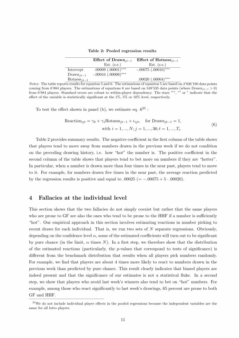
Table 2: Pooled regression results
Effect of Drawnjt−1 Effect of Hotnessjt−1
Est. (s.e.) Est. (s.e.)Intercept .00009 (.00001)∗∗∗ -.00075 (.00010)∗∗∗
Drawnjt−1 -.00044 (.00006)∗∗∗
Hotnessjt−1 .00020 (.00004)∗∗∗
Notes: The table reports results for equation 5 and 6. The estimations of equation 5 are based on 2’826’180 data pointscoming from 6’884 players. The estimations of equations 6 are based on 549’535 data points (where Drawnjt−1 > 0)from 6’884 players. Standard errors are robust to within-player dependency. The stars ∗∗∗, ∗∗ or ∗ indicate that theeffect of the variable is statistically significant at the 1%, 5% or 10% level, respectively.
To test the effect shown in panel (b), we estimate eq. 623 :
Reactionijt = γ0 + γ1Hotnessjt−1 + ǫijt, for Drawnjt−1 = 1,
with i = 1, ..., N ; j = 1, ..., 36; t = 1, ..., Ti.(6)
Table 2 provides summary results. The negative coefficient in the first column of the table shows
that players tend to move away from numbers drawn in the previous week if we do not condition
on the preceding drawing history, i.e. how “hot” the number is. The positive coefficient in the
second column of the table shows that players tend to bet more on numbers if they are “hotter”.
In particular, when a number is drawn more than four times in the near past, players tend to move
to it. For example, for numbers drawn five times in the near past, the average reaction predicted
by the regression results is positive and equal to .00025 (= −.00075 + 5 · .00020).
4 Fallacies at the individual level
This section shows that the two fallacies do not simply coexist but rather that the same players
who are prone to GF are also the ones who tend to be prone to the HHF if a number is sufficiently
“hot”. Our empirical approach in this section involves estimating reactions in number picking to
recent draws for each individual. That is, we run two sets of N separate regressions. Obviously,
depending on the confidence level α, some of the estimated coefficients will turn out to be significant
by pure chance (in the limit, α times N). In a first step, we therefore show that the distribution
of the estimated reactions (particularly, the p-values that correspond to tests of significance) is
different from the benchmark distribution that results when all players pick numbers randomly.
For example, we find that players are about 4 times more likely to react to numbers drawn in the
previous week than predicted by pure chance. This result clearly indicates that biased players are
indeed present and that the significance of our estimates is not a statistical fluke. In a second
step, we show that players who avoid last week’s winners also tend to bet on “hot” numbers. For
example, among those who react significantly to last week’s drawings, 65 percent are prone to both
GF and HHF.
23We do not include individual player effects in the pooled regressions because the independent variables are thesame for all lotto players.
11
As in Section 3, we estimate two separate regression models to capture the GF and the HHF.
We estimate the following two regressions for each player i which explain Reactionijt (defined in
eq. 2) as a function of the recent drawing history:
Reactionijt = β0j + β1iDrawnjt−1 + ǫijt,
with i = 1, ..., N ; j = 1, ..., 36; t = 1, ..., Ti,(7)
and
Reactionijt = γ0j + γ1iHotnessjt−1 + ǫijt, for Drawnjt−1 = 1,
with i = 1, ..., N ; j = 1, ..., 36; t = 1, ..., Ti.(8)
Recall that we operationalize the GF as avoiding numbers drawn in the previous week compared
to numbers not drawn. Hence, for players prone to the GF the effect of Drawnjt in eq. 7 is negative.
We define “Hot hand” players as those who bet more on numbers drawn in the previous week the
“hotter” hey are that are. For these players the effect of Hotnessjt−1 in eq. 8 is thus positive. Note
that we do not expect any effect of Hotnessjt−1 in eq. 8 for “pure” GF players, i.e. those who are
prone to the GF but do not switch to the HHF if a number is sufficiently “hot”. To illustrate,
consider a “pure” GF player who strictly avoids numbers drawn in the previous week. Such a player
has a negative coefficient on Drawnjt−1. But since it is possible to avoid a number only once even
if it is drawn in several consecutive weeks, this player simply stays away from these numbers. This
implies that Reactionijt = 0 when Hotnessjt−1 > 1 such that eq. 8 cannot be estimated for a “pure”
GF player. In addition, eq. 8 cannot be estimated for players who never experience that a number
drawn in the previous week is “hot” (i.e. Hotnessjt−1 > 1) because they do not play frequently.
Section 4.1 shows that players are significantly more likely to react to numbers drawn in the
previous week, and more likely to react to how often a number won in the past, than predicted by
pure chance. In 4.2 we argue that players who are significantly prone to GF also tend to be the
ones who are prone to the HHF.
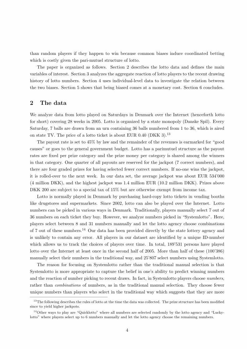
4.1 Fallacy or statistical artifact?
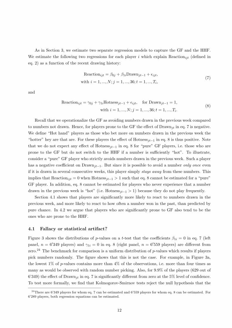
Figure 3 shows the distributions of p-values on a t-test that the coefficients β1i = 0 in eq. 7 (left
panel, n = 6′349 players) and γ1i = 0 in eq. 8 (right panel, n = 6′559 players) are different from
zero.24 The benchmark for comparison is a uniform distribution of p-values which results if players
pick numbers randomly. The figure shows that this is not the case. For example, in Figure 3a,
the lowest 1% of p-values contains more than 4% of the observations, i.e. more than four times as
many as would be observed with random number picking. Also, for 9.9% of the players (629 out of
6’349) the effect of Drawnjt in eq. 7 is significantly different from zero at the 5% level of confidence.
To test more formally, we find that Kolmogorov-Smirnov tests reject the null hypothesis that the
24There are 6’349 players for whom eq. 7 can be estimated and 6’559 players for whom eq. 8 can be estimated. For6’289 players, both regression equations can be estimated.
12
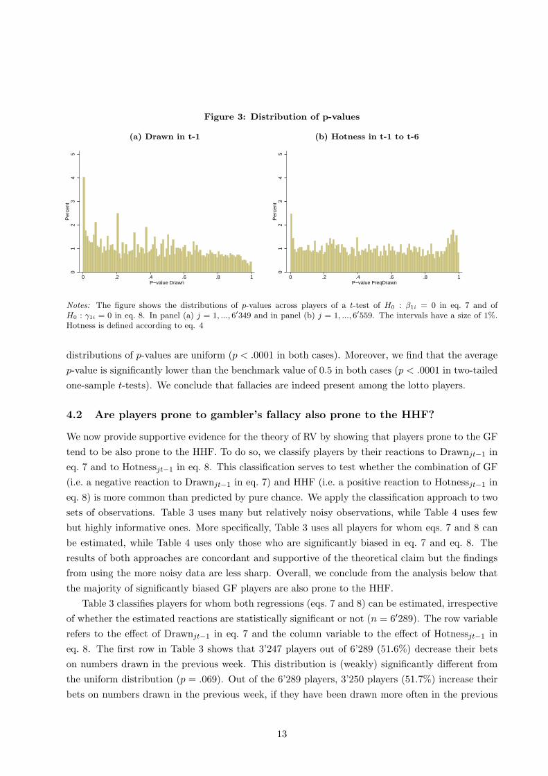
Figure 3: Distribution of p-values
(a) Drawn in t-1
01
23
45
Per
cent
0 .2 .4 .6 .8 1P−value Drawn
(b) Hotness in t-1 to t-6
01
23
45
Per
cent
0 .2 .4 .6 .8 1P−value FreqDrawn
Notes: The figure shows the distributions of p-values across players of a t-test of H0 : β1i = 0 in eq. 7 and ofH0 : γ1i = 0 in eq. 8. In panel (a) j = 1, ..., 6′349 and in panel (b) j = 1, ..., 6′559. The intervals have a size of 1%.Hotness is defined according to eq. 4
distributions of p-values are uniform (p < .0001 in both cases). Moreover, we find that the average
p-value is significantly lower than the benchmark value of 0.5 in both cases (p < .0001 in two-tailed
one-sample t-tests). We conclude that fallacies are indeed present among the lotto players.
4.2 Are players prone to gambler’s fallacy also prone to the HHF?
We now provide supportive evidence for the theory of RV by showing that players prone to the GF
tend to be also prone to the HHF. To do so, we classify players by their reactions to Drawnjt−1 in
eq. 7 and to Hotnessjt−1 in eq. 8. This classification serves to test whether the combination of GF
(i.e. a negative reaction to Drawnjt−1 in eq. 7) and HHF (i.e. a positive reaction to Hotnessjt−1 in
eq. 8) is more common than predicted by pure chance. We apply the classification approach to two
sets of observations. Table 3 uses many but relatively noisy observations, while Table 4 uses few
but highly informative ones. More specifically, Table 3 uses all players for whom eqs. 7 and 8 can
be estimated, while Table 4 uses only those who are significantly biased in eq. 7 and eq. 8. The
results of both approaches are concordant and supportive of the theoretical claim but the findings
from using the more noisy data are less sharp. Overall, we conclude from the analysis below that
the majority of significantly biased GF players are also prone to the HHF.
Table 3 classifies players for whom both regressions (eqs. 7 and 8) can be estimated, irrespective
of whether the estimated reactions are statistically significant or not (n = 6′289). The row variable
refers to the effect of Drawnjt−1 in eq. 7 and the column variable to the effect of Hotnessjt−1 in
eq. 8. The first row in Table 3 shows that 3’247 players out of 6’289 (51.6%) decrease their bets
on numbers drawn in the previous week. This distribution is (weakly) significantly different from
the uniform distribution (p = .069). Out of the 6’289 players, 3’250 players (51.7%) increase their
bets on numbers drawn in the previous week, if they have been drawn more often in the previous
13
Table 3: Classification of all players
Effect of Hotnessjt−1
Effect of Drawnjt−1 Negative Positive Total Fisher p-valueNegative 1570 1677 3247 .188Positive 1469 1573 3042 .191Total 3039 3250 6289 .061Fisher p-value .200 .206 .069
Notes: The table reports numbers of players where β1i < 0 and β1i > 0 in eq. 7 and γ1i < 0 and γ1i > 0 in eq. 8. Itis based on players with at least 30 data points in eqs. 7 and 8 each. The p-values come from Fisher exact tests thatcompare the observed distributions with the uniform distribution.
Table 4: Classification of significantly biased players
Effect of Hotnessjt−t
Effect of Drawnjt−t Negative Positive Total Fisher p-valueNegative 14 60 74 < .0001Positive 8 10 18 1Total 22 70 92 .< .0001Fisher p-value .543 < .0001 < .0001
Notes: The table reports numbers of players where β1i < 0 and β1i > 0 in eq. 7 and γ1i < 0 and γ1i > 0 in eq. 8.It is based on players i for whom H0 : β1i = 0 in eq. 7 and H0 : γ1i = 0 in eq. 8 are rejected at the 5% level. Thep-values come from Fisher exact tests that compare the observed distributions with the uniform distribution.
six weeks. This distribution is also (weakly) significantly different from the uniform distribution
(p = .061). Overall, 1’677 players both decrease bets on numbers drawn in the previous week and
increase bets on numbers that have been drawn frequently in the past six weeks (26.7% compared
to 25% with random picking).
Table 4 shows how GF and HHF relate if we consider players whose estimated reactions in
regressions (eq. 7 and eq. 8) are statistically significant at the 5% level. The classification follows
the same logic as in Table 3, yielding a qualitiatively identical but statistically sharper picture.25
We now find that 80.4% (74 out of 92) decrease their bets on last week’s winners and that 76.1%
(70 out of 92) of players increase their bets on numbers on “hot” numbers. As a result, the
“overlap” between both fallacies is 65% (60 out of 92). Thus, about two thirds of the players under
consideration are prone to both fallacies.
To check whether this “overlap” between both fallacies is not merely a statistical fluke, we test
whether the share of players who exhibit both fallacies (60 out of 92 or 65%) is larger than the
expected share under the assumption that both fallacies are independent. This is indeed the case.
We find that, first, the share of players with GF among those who react significantly to Drawn (but
not necessarily to Hotness) is significantly lower than among players who react significantly to both
Drawn and Hotness. Second, we find that the share of players with HHF among those who react
significantly to Hotness (but not necessarily to Drawn) is significantly lower than among players
25Note that while the absolute number of players for whom both effects (Drawnjt in eq. 7 and Hotnessjt in eq. 8)are significant at the 5% level is rather low (92), it is much higher than the number that would have been observedhad all players chosen numbers randomly. Indeed, 92 is 1.46% of 6’289 and almost 6 times higher than the numberthat would have been observed had all players chosen numbers randomly (0.25% of 6’289 is about 15.7).
14
who react significantly to both Drawn and Hotness (p = .002 in Fisher exact test, in both cases).26
5 Costly fallacies
We now show that holding the belief that lotto numbers can be predicted comes at a monetary cost.
The cost comes in two guises. First, Section 5.1 shows that GF players tend to buy more tickets
than others, and playing the lotto means losing money on average (because the overall payout rate
is only 45%). Second, Section 5.2 shows that biased players win smaller amounts given that they
happen to win. Note that biased players are just as likely as non-biased players to win, i.e. to guess
x numbers correctly. Their problem is that they tend to win in the “wrong weeks” because their
individual prize money for guessing x numbers correctly is lower: due to the pari-mutuel nature of
lotto they have to share the prize money with many other (biased) players.
5.1 Biased players lose more
We now show that players significantly prone to the GF buy more tickets than other players. To
do so, we regress the average number of tickets bought in Systemlotto on the variables indicating a
bias as defined in Section 4 in a robust regression. In particular, we measure whether players who
move away from numbers buy more tickets than those who move toward numbers, by including
“Drawn Neg” in the regression, which is a binary variable equal to one for player i if β1i < 0 in eq.
7 and equal to zero if β1i > 0. We also include the variable “Drawn Sig”, which indicates whether
H0 : β1i = 0 in eq. 7 is rejected at the 5% level for player i or not (0/1), and the interaction
between both. Including the interaction allows us to test whether players prone to the GF — those
who bet less on last week’s winners — buy more tickets than other players. Similarly, to study
whether players who increase their bets on “hot” numbers buy more tickets we include the variable
“Hotness Pos”, which is a binary variable equal to one for player i if γ1i > 0 and equal to zero if
γ1i < 0, the variable “Hotness Sig”, and the interaction between both. We also include controls for
gender, age, and the average number of lotto numbers picked.27 Including the latter is important
to avoid upwardly biased estimates for two reasons. First, because players who pick more lotto
numbers are more likely to move away from a number than players who pick fewer lotto numbers
— simply because there are more numbers to potentially move away from — and thus also more
likely to have β1i < 0 in eq. 7. Second, because the number of lotto numbers picked is positively
26The share of players with GF among those who react significantly to Drawn irrespective of whether they reactsignificantly to Hotness is 64% (403 out of 629 vs. 74 out of 92, or 80%). The share of players with HHF among thosewho react significantly to Hotness irrespective of whether they react significantly to Drawn is 59% (264 out of 448vs. 70 out of 92, or 76%).
27The individual characteristics we have are gender, age and postal code. We experimented with regressions thatinclude variables related to the estimation results of eq. 8, where the effect of Hotnessjt−1 on Reactionijt is estimated.For example, we included whether or not γ1i > 0 as a dummy regressor in a regression where the average number oftickets bought is the dependent variable. However, none of the variables related to eq. 8 turned out to be significantlycorrelated with the average number of tickets bought by Systemlotto players.
15

Table 5: Regression of number of tickets bought
Dep. var.: (1) (2)Avg. # tickets bought Est. (s.e.) Est. (s.e.)Intercept 11.69 (1.28)∗∗∗ 12.11 (1.31)∗∗∗
Drawn Neg 0.72 (0.51) -0.11 (0.71)Drawn Sig -1.69 (1.32) 1.66 (1.32)Drawn Neg x Drawn Sig 5.05 (1.68)∗∗∗ 4.96 (1.68)∗∗∗
Hotness Pos 0.07 (0.50) -0.75 (0.70)Hotness Sig 1.00 (1.48) 1.07 (1.48)Hotness Pos x Hotness Sig -2.32 (1.75) -2.42 (1.95)Drawn Neg x Hotness Pos 1.62 (0.96)∗
Male 3.95 (0.68)∗∗∗ 3.96 (0.68)∗∗∗
Age -0.13 (0.02)∗∗∗ -0.13 (0.02)∗∗∗
Avg. # numbers picked 1.27 (0.02)∗∗∗ 1.27 (0.02)∗∗∗
N 6288 6288Notes: The table reports results from robust regressions (Stata command rreg) where the dependent variable is theaverage number of tickets bought by player i through the Systemlotto device. Drawn Neg = 1 for player i if β1i < 0in eq. 7 and 0 otherwise. Drawn Sig = 1 if H0 : β1i = 0 in eq. 7 is rejected at the 5% level for player i and 0 otherwise.Hotness Pos = 1 for player i if γ1i > 0 in eq. 8 and 0 otherwise. Hotness Sig = 1 if H0 : γ1i = 0 in eq. 8 is rejected atthe 5% level for player i and 0 otherwise. The stars ∗∗∗, ∗∗ or ∗ indicate that the effect of the variable is statisticallysignificant at the 1%, 5% or 10% level, respectively.
correlated with the number of tickets bought (see Appendix A2). Leaving out this control variable
thus induces upward bias on the regression coefficient of Drawn Neg.
Table 5 shows that players who are significantly prone to GF buy significantly more tickets
than other players. This conclusion emerges from the fact that the interaction between Drawn Neg
and Drawn Sig is highly significant, whereas Drawn Neg is not. According to specification (1), GF
players buy about 4 tickets more (= 0.72− 1.69 + 5.05) or bet about 1.6 EUR more in an average
week (this is significantly different from zero with p < 0.001). Compared to the median player,
this is about 20% more. In contrast, players who are significantly prone to the HHF — who bet
more on “hot” numbers — do not buy more tickets (see insignificant coefficient on Hotness Pos).
Specification (2) includes the interaction between “Drawn Neg” and “Hotness Pos” to test whether
players who react in line with both the GF and the HHF buy more tickets than other players. We
find that this is the case. The effect of Drawn Neg x Hotness Pos in specification (2) is weakly
significant which suggests that such players tend to buy more lotto tickets than other players (about
1.6 tickets more). Note that the results for GF players discussed in specification (1) are robust to
the inclusion of this interaction effect in specification (2).
Table 5 further shows in both specifications that male players buy more tickets than female
players, while older players buy fewer tickets. For example, men buy about 4 tickets (i.e. bet 1.6
EUR) more per week than women, and a typical 60-year old player buys about 5 tickets less than
a typical 20-year old one. The regression also shows that, as expected, those who buy many tickets
also tend to pick many numbers.
One hypothesis is that overconfidence might drive our result that players who react significantly
in line with the GF buy significantly more tickets. This resonates well with the fact that the
16
GF results are driven by male players28, and males have been found to be particularly prone to
overconfidence (see, e.g., Niederle and Vesterlund, 2007).
5.2 Biased players win less
Given that it is not possible for lotto players to increase the probability of winning per ticket
purchased, the best they can do is to maximize the amount won if they happen to win. Winnings
are maximized by avoiding popular numbers and combinations. The reason is that because of
the pari-mutuel structure of lotto, picking popular numbers entails the risk of having to share the
prize with many other players. Thus, being biased is costly if the bias is common. Observing that
unexpectedly many players pick the same numbers can be due to a bias as studied in this paper or
to using particular visual patterns to pick numbers on a lotto ticket. For example, Simon (1999)
shows that picking the least popular combinations yields a gain that is more than four times higher
than the one resulting from picking the most popular combinations in UK lotto.
We now show that biased players win lower amounts than players who pick numbers randomly,
given that they happen to guess x numbers right. Note that by comparing payoffs conditional on
winning, we effectively isolate the effect of picking popular numbers from the effect of pure luck,
provided that the number of observations is sufficiently large. Yet, winning the jackpot is very
unlikely (about 1 in 8 million) and the chances are rather low even for 6 correct numbers. As a
consequence, there are not many observations in these prize categories (24 in our dataset) which
implies that the effect of pure luck on the payoff of lotto players is quite high in these categories.
Hence, we refrain from investigating the difference for 6 and 7 correct numbers.29 Focusing on
small prizes obviously implies that the estimated absolute cost of biases is low, and our estimates
are thus likely to be a lower bound for the cost of being biased which results from winning less
money if a player happens to win.
We show that being biased is costly for the subset of players for whom we have information on
the combinations chosen by the lotto agency on behalf of these players (i.e. players using system M,
see Appendix A.2). As a benchmark, we calculate the expected prize of players picking numbers
randomly by means of Monte Carlo simulations. In these simulations we use the fact that a random
player has the same probability of winning in all weeks. Our result suggests that biased players
tend to win in the “wrong” weeks, when many winners share the prize.
Table 6 shows that biased players indeed win less than a player who picks numbers randomly.30
The first column shows the average winning of a random player (DKK 42.57 for 4 correct and DKK
149.6 for 5 correct). The second column shows that players with β1i < 0 (whether significant or
not), i.e. those that tend to avoid numbers drawn in the previous week win DKK 42.47 and DKK
28Suetens and Tyran (2012) show that, in the aggregate, men are prone to the GF whereas women are not.29The prizes in the lotto vary quite considerably over time. For example, the prize for guessing 6 numbers correctly
was between 18’000 DKK and 113’000 DKK with a mean of 66’000 DKK in our dataset.30The numbers of observations reported in Table 6 do not refer to numbers of players, but to numbers of winnings
from predicting four or five times correctly.
17
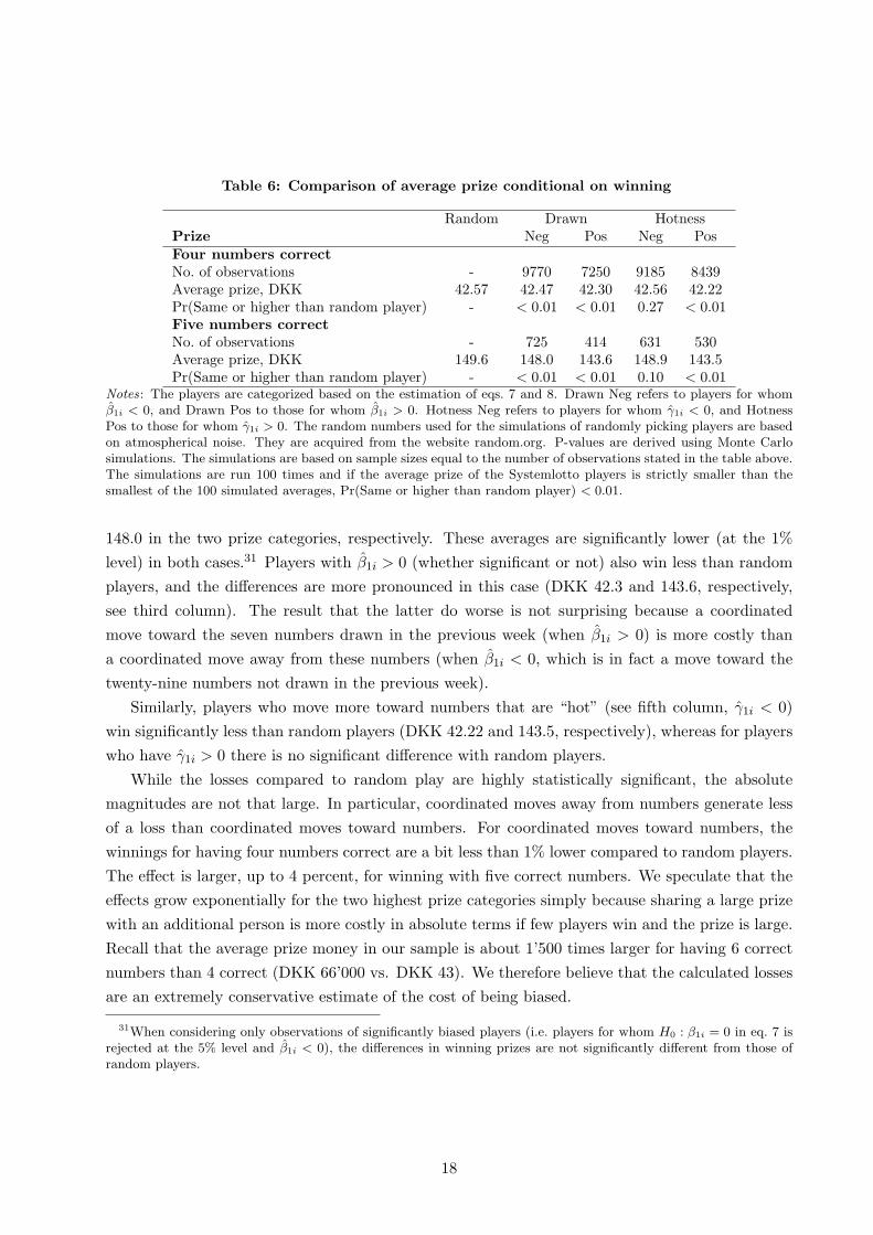
Table 6: Comparison of average prize conditional on winning
Random Drawn HotnessPrize Neg Pos Neg PosFour numbers correct
No. of observations - 9770 7250 9185 8439Average prize, DKK 42.57 42.47 42.30 42.56 42.22Pr(Same or higher than random player) - < 0.01 < 0.01 0.27 < 0.01Five numbers correct
No. of observations - 725 414 631 530Average prize, DKK 149.6 148.0 143.6 148.9 143.5Pr(Same or higher than random player) - < 0.01 < 0.01 0.10 < 0.01
Notes: The players are categorized based on the estimation of eqs. 7 and 8. Drawn Neg refers to players for whomβ1i < 0, and Drawn Pos to those for whom β1i > 0. Hotness Neg refers to players for whom γ1i < 0, and HotnessPos to those for whom γ1i > 0. The random numbers used for the simulations of randomly picking players are basedon atmospherical noise. They are acquired from the website random.org. P-values are derived using Monte Carlosimulations. The simulations are based on sample sizes equal to the number of observations stated in the table above.The simulations are run 100 times and if the average prize of the Systemlotto players is strictly smaller than thesmallest of the 100 simulated averages, Pr(Same or higher than random player) < 0.01.
148.0 in the two prize categories, respectively. These averages are significantly lower (at the 1%
level) in both cases.31 Players with β1i > 0 (whether significant or not) also win less than random
players, and the differences are more pronounced in this case (DKK 42.3 and 143.6, respectively,
see third column). The result that the latter do worse is not surprising because a coordinated
move toward the seven numbers drawn in the previous week (when β1i > 0) is more costly than
a coordinated move away from these numbers (when β1i < 0, which is in fact a move toward the
twenty-nine numbers not drawn in the previous week).
Similarly, players who move more toward numbers that are “hot” (see fifth column, γ1i < 0)
win significantly less than random players (DKK 42.22 and 143.5, respectively), whereas for players
who have γ1i > 0 there is no significant difference with random players.
While the losses compared to random play are highly statistically significant, the absolute
magnitudes are not that large. In particular, coordinated moves away from numbers generate less
of a loss than coordinated moves toward numbers. For coordinated moves toward numbers, the
winnings for having four numbers correct are a bit less than 1% lower compared to random players.
The effect is larger, up to 4 percent, for winning with five correct numbers. We speculate that the
effects grow exponentially for the two highest prize categories simply because sharing a large prize
with an additional person is more costly in absolute terms if few players win and the prize is large.
Recall that the average prize money in our sample is about 1’500 times larger for having 6 correct
numbers than 4 correct (DKK 66’000 vs. DKK 43). We therefore believe that the calculated losses
are an extremely conservative estimate of the cost of being biased.
31When considering only observations of significantly biased players (i.e. players for whom H0 : β1i = 0 in eq. 7 isrejected at the 5% level and β1i < 0), the differences in winning prizes are not significantly different from those ofrandom players.
18
6 Discussion
Given that lotto drawings are truly random, it seems absurd to believe that anyone can predict
next week’s numbers. Yet, our data suggests that the lotto players studied here hold such beliefs
and, curiously enough, the lotto agency itself describes the lotto as: “a number game which is about
predicting the correct numbers drawn” (translated from danskespil.dk, see “rules of the game”).
Our data is unique in that we track individual players’ choices, enabling us to provide unusually
clean evidence on the gambler’s fallacy and the hot hand fallacy, and to investigate whether they
relate as predicted by recent economic theory in a natural context where stakes are substantial.
In the aggregate, we find that bets on a lotto number are reduced after a number has been
drawn (consistent with the gambler’s fallacy), but players tend to bet more on numbers that have
won frequently in recent draws (consistent with the hot hand fallacy). It is rather remarkable
that we find evidence for these fallacies in the aggregate given the pari-mutuel nature of lotto.
If anything, lotto is not about predicting the numbers drawn — because all numbers are equally
likely — but about predicting numbers picked by others — because picking the same numbers
as others do reduces the amount won given that a player happens to win. But biased players
seem not be aware of this fact. We indeed find that biased players — particularly those prone to
the hot hand fallacy — win lower amounts than players who pick numbers randomly, given that
they happen to win a prize. The gambler’s fallacy seems to come mostly at another cost: it is
related to higher expenditures on lotto tickets. Spending more on lotto tickets means losing more
money on average because the statutory payout rate is 45 percent of revenues only. But spending
more on lotto potentially also results in substantial economic costs since increased expenditures
on lotto tickets are financed to a large extent by cutting expenditures on food, rent or mortgages
(Kearney, 2005). Since lotto gambling is to some extent addictive (Guryan and Kearney, 2010),
biases may have quite some influence on welfare. At the individual level, we find that the same
lotto players who are prone to the gambler’s fallacy also tend to be prone to the hot hand fallacy.
This finding lends support to the recent behavioral model by Rabin and Vayanos (2010) from a
novel angle. It complements evidence from the lab (Asparouhova et al. (2009)) and from financial
markets (Loh and Warachka (2012)).
The evidence we provide for the existence of biased inference from noisy data is potentially
relevant for a number of anomalies that seem to be common in financial decision making and fi-
nancial markets. For example, they could explain why investors seem to have a willingness to pay
for “expert” predictions of investment performance (Powdthavee and Riyanto, 2012) and, if suffi-
ciently prevalent, also for the emergence of underreaction of stock prices to news but overreaction
to a series of news, particularly if driven by small investors (e.g. Hvidkjaer, 2006). While it is
not clear that evidence from lotto gambling with its limited possibilities to engage in arbitrage
(rational investors may compensate the behavior of irrational ones such that no effect is observed
in the aggregate, e.g. Fehr and Tyran, 2005) extrapolate to financial markets, it does not seem
entirely implausible that such biases may manifest themselves at least in some financial markets.
For example, people who play lotto also seem to be likely to invest in lotto-type stocks, such as
19
low-priced stocks with high idiosyncratic volatility and skewness (Kumar, 2009).
Unfortunately, biases and fallacies are hard to unambiguously pin down in financial markets
because the data generating process is fundamentally unknown, market interaction may multiply
or mitigate the effects of biases in the aggregate, and structural breaks or regime shifts may occur.
In the experimental laboratory, the data generating process is tightly controlled, and fallacies can
in principle be clearly pinned down at the individual level. But evidence from the experimental
laboratory has been claimed to be difficult to extrapolate to investor behavior “in the field” because
the lab tends to be somewhat artificial, participants in an experiment know they are being observed,
and stakes are often small (see Camerer, 2011, for a general discussion). Data from lotto gambling
is complementary to these approaches because playing the lotto is natural to many, lotto has a
known, tightly controlled and transparent random process, and substantial amounts are at stake.
We therefore think that our study importantly complements evidence coming from financial markets
and the laboratory, respectively.
20
References
Asparouhova, E., Hertzel, M., and Lemmon, M. (2009). Inference from streaks in random outcomes:
experimental evidence on beliefs in regime shifting and the law of small numbers. Management
Science, 55:1766–1782.
Bar-Eli, M., Avugos, S., and Raab, M. (2006). Twentyy years of hot hand research: Review and
critique. Psychology of Sport and Exercise, 7:525–553.
Bar-Hillel, M. and Wagenaar, W. (1991). The perception of randomness. Advances in Applied
Mathematics, 12:428–454.
Barberis, N., Shleifer, A., and Vishny, R. (1998). A model of investor sentiment. Journal of
Financial Economics, 49:307–343.
Camerer, C. (1989). Does the basketball market believe in the hot hand? American Economic
Review, 79:1257–1261.
Camerer, C. (2011). The promise and success of lab-field generalizability in experimental economics:
A critical reply to Levitt and List. Technical report, California Institute of Technology.
Carhart, M. (1997). On persistence in mutual fund performance. Journal of Finance, 52:57–82.
Clotfelder, C. and Cook, P. (1993). The “gambler’s fallacy” in lottery play. Management Science,
39:1521–1525.
Cohen, L. and Frazzini, A. (2008). Economic links and predictable returns. Journal of Finance,
63:1977–2011.
Croson, R. and Sundali, J. (2005). The gambler’s fallacy and the hot hand: Empirical data from
casinos. Journal of Risk and Uncertainty, 30:195–209.
Cutler, D., Poterba, J., and Summers, L. (1991). Speculative dynamics. Review of Economic
Studies, 58:529–546.
Daniel, K., Hirshleifer, D., and Subrahmanyam, A. (1998). Investor psychology and security market
under- and overreactions. Journal of Finance, 53:1839–1885.
De Bondt, W. and Thaler, R. (1985). Does the stock market overreact? Journal of Finance,
40:793–805.
De Bondt, W. and Thaler, R. (1987). Further evidence on investor overreaction and stock market
seasonality. Journal of Finance, 42:557–581.
DellaVigna, S. and Pollet, J. (2009). Investor inattention and Friday earnings announcements.
Journal of Finance, 64:709–749.
Fehr, E. and Tyran, J.-R. (2005). Individual irrationality and aggregate outcomes. Journal of
Economic Perspectives, 19:43–66.
Gilovich, T., Vallone, R., and Tversky, A. (1985). The hot hand in basketball: On the misperception
of random sequences. Cognitive Psychology, 17:295–314.
Guryan, J. and Kearney, M. (2008). Gambling at lucky stores: Empirical evidence from state
lottery sales. American Economic Review, 98:458–473.
Guryan, J. and Kearney, M. (2010). Is lottery gambling addictive? American Economic Journal:
Economic Policy, 2:90–110.
21
Hendricks, D., Patel, J., and Zeckhauser, R. (1993). Hot hands in mutual funds: Short-run persis-
tence of performance. Journal of Finance, 48:93–130.
Hirshleifer, D., Lim, S., and Teoh, S. (2009). Drive to distraction: Extraneous events and underre-
action to earnings news. Journal of Finance, 64:2289–2326.
Hong, H. and Stein, J. C. (1999). A unified theory of underreaction, momentum trading, and
overreaction in asset markets. Journal of Finance, 54:2143–2184.
Huber, J., Kirchler, M., and Stockl, T. (2010). The hot hand belief and the gambler’s fallacy in
investment decisions under risk. Theory and Decision, 68:445–462.
Hvidkjaer, S. (2006). A trade-based analysis of momentum. Journal of Financial Studies, 19:457–
491.
Jagannathan, R., Malakhov, A., and Novikov, D. (2010). Do hot hands exist among hedge fund
managers? An empirical evaluation. Journal of Finance, 65:215–255.
Jegadeesh, N. and Titman, S. (1993). Returns to buying winners and selling losers: implications
for stock market efficiency. Journal of Finance, 48:65–91.
Kearney, M. (2005). State lotteries and consumer behavior. Journal of Public Economics, 89:2269–
2299.
Kumar, A. (2009). Who gambles in the stock market? Journal of Finance, 64:1889–1933.
Laplace, P. (1812). A philosophical essay on probabilities. Translated by F.W. Truscott and F.L.
Emory from Essai philosophique sur les probabilites, 1902.
Loh, R. and Warachka, M. (2012). Streaks in earnings surprises and the cross-section of stock
returns. Management Science, 58:1305–1321.
Niederle, M. and Vesterlund, L. (2007). Do women shy away from competition? Do men compete
too much? Quarterly Journal of Economics, 122:1067–1101.
Offerman, T. and Sonnemans, J. (2004). What’s causing overreaction? An experimental investiga-
tion of recency and the hot-hand effect. Scandinavian Journal of Economics, 106:533–553.
Oskarsson, A., van Boven, L., McClelland, G., and Hastie, R. (2009). What’s next? Judging
sequences of binary events. Psychological Bulletin, 135:262–285.
Poterba, J. and Summers, L. (1988). Mean reversion in stock prices: Evidence and implications.
Journal of Financial Economics, 22:27–59.
Powdthavee, N. and Riyanto, Y. (2012). Why do people pay for useless advice? Implications of
gamblers and hot-hand fallacies in a false-expert setting. Discussion Paper 6557, IZA.
Rabin, M. (2002). Inference by believers in the law of small numbers. Quarterly Journal of
Economics, 117:775–816.
Rabin, M. and Vayanos, D. (2010). The gambler’s and hot-hand fallacies: Theory and applications.
Review of Economic Studies, 77:730–778.
Rapoport, A. and Budescu, D. (1997). Randomization in individual choice behavior. Psychological
Review, 104:603–617.
Simon, J. (1999). An analysis of the distribution of combinations chosen by UK national lottery
players. Journal of Risk and Uncertainty, 17:243–276.
22
Suetens, S. and Tyran, J.-R. (2012). The gambler’s fallacy and gender. Journal of Economic
Behavior & Organization, 83:118–124.
Sundali, J. and Croson, R. (2006). Biases in casino betting: The hot hand and the gambler’s fallacy.
Judgment and Decision Making, 1:1–12.
Terrell, D. (1994). A test of the gambler’s fallacy: Evidence from pari-mutuel games. Journal of
Risk and Uncertainty, 8:309–317.
Tversky, A. and Kahneman, D. (1971). Belief in the law of small numbers. Psychological Bulletin,
76:105–110.
Yaari, G. and David, G. (2012). “Hot hand” on strike: Bowling data indicates correlation to recent
past results, not causality. PLoS ONE, 7:e30112.
23
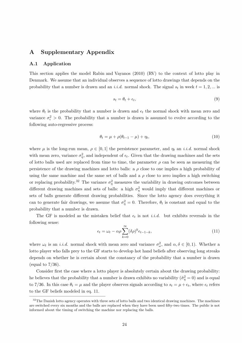
A Supplementary Appendix
A.1 Application
This section applies the model Rabin and Vayanos (2010) (RV) to the context of lotto play in
Denmark. We assume that an individual observes a sequence of lotto drawings that depends on the
probability that a number is drawn and an i.i.d. normal shock. The signal st in week t = 1, 2, ... is
st = θt + ǫt, (9)
where θt is the probability that a number is drawn and ǫt the normal shock with mean zero and
variance σ2ǫ > 0. The probability that a number is drawn is assumed to evolve according to the
following auto-regressive process:
θt = µ+ ρ(θt−1 − µ) + ηt, (10)
where µ is the long-run mean, ρ ∈ [0, 1] the persistence parameter, and ηt an i.i.d. normal shock
with mean zero, variance σ2η, and independent of ǫt. Given that the drawing machines and the sets
of lotto balls used are replaced from time to time, the parameter ρ can be seen as measuring the
persistence of the drawing machines and lotto balls: a ρ close to one implies a high probability of
using the same machine and the same set of balls and a ρ close to zero implies a high switching
or replacing probability.32 The variance σ2η measures the variability in drawing outcomes between
different drawing machines and sets of balls: a high σ2η would imply that different machines or
sets of balls generate different drawing probabilities. Since the lotto agency does everything it
can to generate fair drawings, we assume that σ2η = 0. Therefore, θt is constant and equal to the
probability that a number is drawn.
The GF is modeled as the mistaken belief that ǫt is not i.i.d. but exhibits reversals in the
following sense:
ǫt = ωt − αρ∞∑
k=0
(δρ)kǫt−1−k, (11)
where ωt is an i.i.d. normal shock with mean zero and variance σ2ω, and α, δ ∈ [0, 1). Whether a
lotto player who falls prey to the GF starts to develop hot hand beliefs after observing long streaks
depends on whether he is certain about the constancy of the probability that a number is drawn
(equal to 7/36).
Consider first the case where a lotto player is absolutely certain about the drawing probability:
he believes that the probability that a number is drawn exhibits no variability (σ2η = 0) and is equal
to 7/36. In this case θt = µ and the player observes signals according to st = µ+ ǫt, where ǫt refers
to the GF beliefs modeled in eq. 11.
32The Danish lotto agency operates with three sets of lotto balls and two identical drawing machines. The machinesare switched every six months and the balls are replaced when they have been used fifty-two times. The public is notinformed about the timing of switching the machine nor replacing the balls.
24
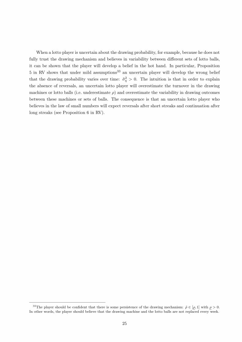
When a lotto player is uncertain about the drawing probability, for example, because he does not
fully trust the drawing mechanism and believes in variability between different sets of lotto balls,
it can be shown that the player will develop a belief in the hot hand. In particular, Proposition
5 in RV shows that under mild assumptions33 an uncertain player will develop the wrong belief
that the drawing probability varies over time: σ2η > 0. The intuition is that in order to explain
the absence of reversals, an uncertain lotto player will overestimate the turnover in the drawing
machines or lotto balls (i.e. underestimate ρ) and overestimate the variability in drawing outcomes
between these machines or sets of balls. The consequence is that an uncertain lotto player who
believes in the law of small numbers will expect reversals after short streaks and continuation after
long streaks (see Proposition 6 in RV).
33The player should be confident that there is some persistence of the drawing mechanism: ρ ∈ [ρ, 1] with ρ > 0.In other words, the player should believe that the drawing machine and the lotto balls are not replaced every week.
25
A.2 Overview of the different systems in Systemlotto
Option Type of system # chosen numbers in a set # tickets/combinations generated
1 M 8 8
2 M 9 36
3 M 10 120
4 M 11 330
5 M 12 792
6 R 10 8
7 R 10 30
8 R 11 20
9 R 11 34
10 R 12 12
11 R 12 24
12 R 12 48
13 R 13 18
14 R 13 66
15 R 14 48
16 R 14 132
17 R 15 24
18 R 15 69
19 R 16 32
20 R 16 109
21 R 16 240
22 R 17 272
23 R 18 82
24 R 19 338
25 R 20 450
26 R 20 1040
27 R 21 198
28 R 23 345
29 R 24 455
30 R 25 600
31 C 17 17
32 C 18 33
33 C 19 52
34 C 20 20
35 C 20 80
36 C 22 60
37 C 24 24
38 C 24 120
39 C 25 100
40 C 25 200
41 C 28 194
42 C 30 268
43 C 31 155
Notes: Under system “M” all potential combinations of the chosen numbers in a set are generated. Systems “R”and ‘C” are both reduced systems, in which only some of the potential combinations are generated. Systems “C”are more heavily reduced than systems “R”. That is, a smaller share of the potential combinations are generated insystems “C” than in systems “R”.
26
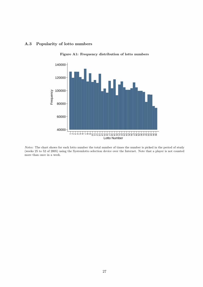
A.3 Popularity of lotto numbers
Figure A1: Frequency distribution of lotto numbers
40000
60000
80000
100000
120000
140000
Fre
quen
cy
1 2 3 4 5 6 7 8 9 10 11 12 13 14 15 16 17 18 19 20 21 22 23 24 25 26 27 28 29 30 31 32 33 34 35 36
Lotto Number
Notes: The chart shows for each lotto number the total number of times the number is picked in the period of study(weeks 25 to 52 of 2005) using the Systemlotto selection device over the Internet. Note that a player is not countedmore than once in a week.
27
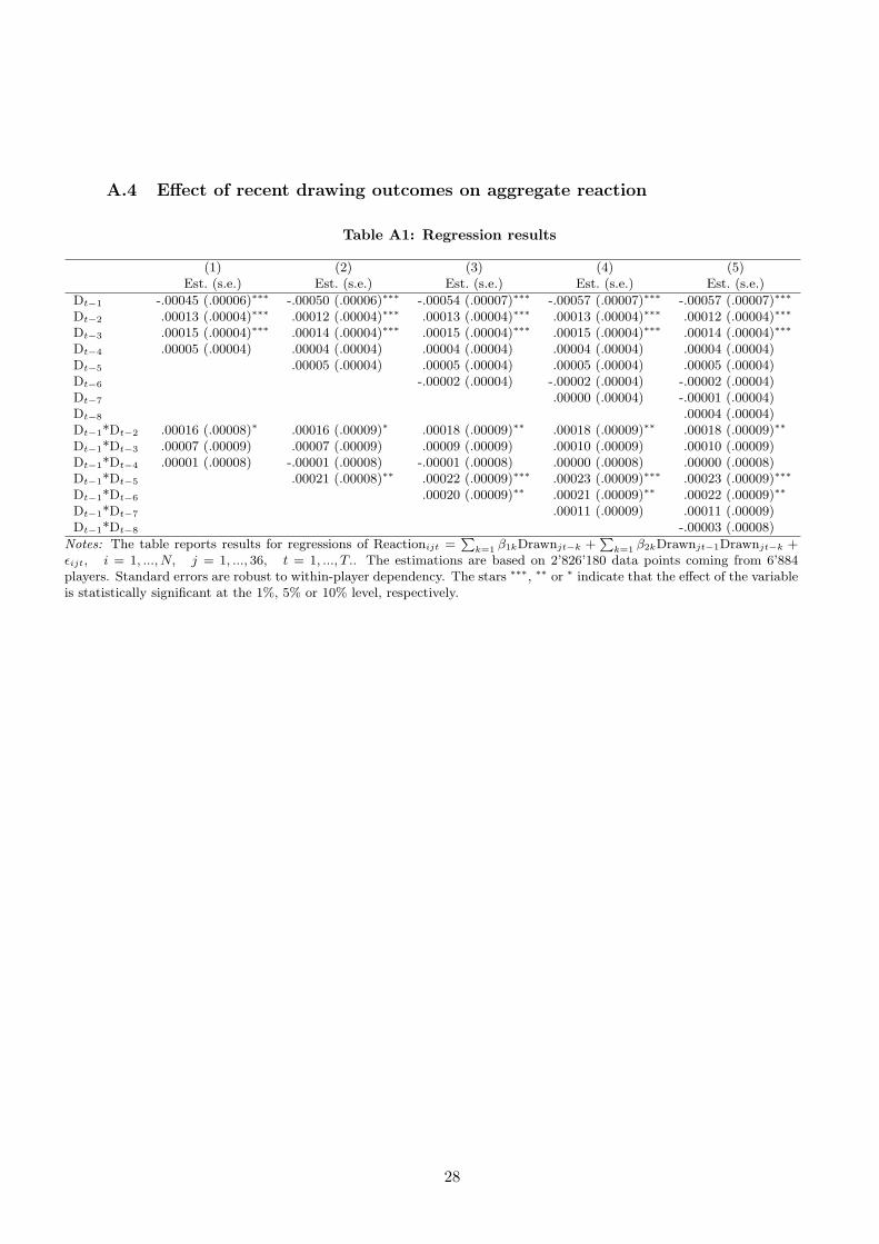
A.4 Effect of recent drawing outcomes on aggregate reaction
Table A1: Regression results
(1) (2) (3) (4) (5)Est. (s.e.) Est. (s.e.) Est. (s.e.) Est. (s.e.) Est. (s.e.)
Dt−1 -.00045 (.00006)∗∗∗ -.00050 (.00006)∗∗∗ -.00054 (.00007)∗∗∗ -.00057 (.00007)∗∗∗ -.00057 (.00007)∗∗∗
Dt−2 .00013 (.00004)∗∗∗ .00012 (.00004)∗∗∗ .00013 (.00004)∗∗∗ .00013 (.00004)∗∗∗ .00012 (.00004)∗∗∗
Dt−3 .00015 (.00004)∗∗∗ .00014 (.00004)∗∗∗ .00015 (.00004)∗∗∗ .00015 (.00004)∗∗∗ .00014 (.00004)∗∗∗
Dt−4 .00005 (.00004) .00004 (.00004) .00004 (.00004) .00004 (.00004) .00004 (.00004)Dt−5 .00005 (.00004) .00005 (.00004) .00005 (.00004) .00005 (.00004)Dt−6 -.00002 (.00004) -.00002 (.00004) -.00002 (.00004)Dt−7 .00000 (.00004) -.00001 (.00004)Dt−8 .00004 (.00004)Dt−1*Dt−2 .00016 (.00008)∗ .00016 (.00009)∗ .00018 (.00009)∗∗ .00018 (.00009)∗∗ .00018 (.00009)∗∗
Dt−1*Dt−3 .00007 (.00009) .00007 (.00009) .00009 (.00009) .00010 (.00009) .00010 (.00009)Dt−1*Dt−4 .00001 (.00008) -.00001 (.00008) -.00001 (.00008) .00000 (.00008) .00000 (.00008)Dt−1*Dt−5 .00021 (.00008)∗∗ .00022 (.00009)∗∗∗ .00023 (.00009)∗∗∗ .00023 (.00009)∗∗∗
Dt−1*Dt−6 .00020 (.00009)∗∗ .00021 (.00009)∗∗ .00022 (.00009)∗∗
Dt−1*Dt−7 .00011 (.00009) .00011 (.00009)Dt−1*Dt−8 -.00003 (.00008)
Notes: The table reports results for regressions of Reactionijt =∑
k=1 β1kDrawnjt−k +∑
k=1 β2kDrawnjt−1Drawnjt−k +ǫijt, i = 1, ..., N, j = 1, ..., 36, t = 1, ..., T.. The estimations are based on 2’826’180 data points coming from 6’884players. Standard errors are robust to within-player dependency. The stars ∗∗∗, ∗∗ or ∗ indicate that the effect of the variableis statistically significant at the 1%, 5% or 10% level, respectively.
28